An emulator for the Lyman-$\alpha$ forest in beyond-$\Lambda$CDM cosmologies

Abstract

Interpreting observations of the Lyman-$\alpha$ forest flux power spectrum requires interpolation between a small number of expensive simulations. We present a Gaussian process emulator modelling the 1D flux power spectrum as a function of the amplitude and slope of the small-scale linear matter power spectrum, and the state of the intergalactic medium at the epoch of interest ($2<z<4$). This parameterisation enables the prediction of the flux power spectrum in extended cosmological models that are not explicitly included in the training set, eliminating the need to construct bespoke emulators for a number of extensions to $\Lambda$CDM. Our emulator is appropriate for cosmologies in which the linear matter power spectrum is described to percent level accuracy by just an amplitude and slope across the epoch of interest, and in the regime probed by eBOSS/DESI data. We demonstrate this for massive neutrino cosmologies, where the emulator is able to predict the flux power spectrum in a $\Sigma m_{\nu}=0.3$ eV neutrino cosmology to sub-percent accuracy, without including massive neutrinos in the training simulations. Further parameters would be required to describe models with sharp features in the linear power, such as warm or light axion dark matter. This work will facilitate the combination of upcoming DESI data with observations of the cosmic microwave background, to obtain constraints on neutrino mass and other extensions to $\Lambda$CDM cosmology.

1 Introduction

The Lyman-$\alpha$ forest (Ly$\alpha$ forest) is a series of absorption features in the spectra of high-redshift quasars, which is caused by the presence of intervening neutral hydrogen. During the last decade, the Baryon Oscillation Spectroscopic Survey (BOSS, [1]) and its extension eBOSS [2] have obtained over 200,000 quasar spectra. These surveys were able to measure the 3D correlation of absorption features and detect baryon acoustic oscillations (BAO) around $z=2.3$ [3]. In addition, the same dataset has been used to provide precise measurements of the flux power spectrum along the line of sight, $P_{\mathrm{1D}}$ [4, 5]. In this paper we present a framework to interpret these $P_{\mathrm{1D}}$ measurements and obtain robust constraints on cosmological parameters. Starting in 2021, the Dark Energy Spectroscopic Instrument (DESI, [6]) will observe 700,000 Ly$\alpha$ forest quasar spectra, and will provide the most precise measurement of the $P_{\mathrm{1D}}$ to date. $P_{\mathrm{1D}}$ measurements are a unique probe of the clustering of matter on megaparsec scales [7, 8, 9, 10, 11, 12, 13]. In particular, measurements from BOSS, eBOSS and DESI are sensitive to the clustering of matter on scales of $0.2\,\mathrm{Mpc}^{-1}<k<3\,\mathrm{Mpc}^{-1}$ [22]. This information is highly complementary to other probes, such as observations of the cosmic microwave background (CMB), and combined analyses have provided some of the tightest constraints on the shape of the primordial power spectrum and upper limits on the neutrino mass scale [23, 24, 25, 26, 27, 28, 29, 30, 31, 32].

Obtaining cosmological constraints from $P_{\mathrm{1D}}$ measurements requires theoretical modelling. Perturbative approaches are not sufficiently accurate on the small scales to which the $P_{\mathrm{1D}}$ is sensitive. Moreover, the absorption features are also sensitive to the state of the intergalactic medium (IGM), which is dependent on baryonic physics and the ultra-violet background [33]. Modelling these effects simultaneously requires expensive hydrodynamical simulations, each costing $\sim 10^{5}$ CPU hours, which means, in practice, that only a small number ($\lesssim 100$) of simulations can be run for a given analysis. This is far fewer than the $\sim 10^{6}$ likelihood evaluations necessary for common sampling techniques, e.g., Markov chain Monte Carlo methods (MCMC), to provide robust statistical constraints on parameters. A solution to this problem has been to construct frameworks that interpolate between simulations. Similar problems exist in other areas of cosmology, such as in analysis of galaxy surveys, where Gaussian processes have been used to interpolate probabilistically (or emulate) the galaxy power spectrum [34] and correlation function [35] as functions of cosmology from a small number of expensive simulations. Analysis of the $P_{\mathrm{1D}}$ over the last decade most commonly used quadratic polynomial interpolation [36, 37]; however recent work has demonstrated the advantages of using a Gaussian process emulator to perform the interpolation [15, 38, 39, 40, 41, 20, 21].

Historically, approaches to combining small-scale clustering information from the Ly$\alpha$ forest with CMB observations fall into two categories. Early work on the Ly$\alpha$ forest recognised that the Ly$\alpha$ forest probes the universe at an epoch that is close to an Einstein de-Sitter (EdS) model, and therefore considered the cosmological information in the Ly$\alpha$ forest to be concentrated in the linear matter power spectrum [7, 9, 11, 10]. The procedure was then to constrain the $z\sim 3$, linear matter power spectrum on megaparsec scales from Ly$\alpha$ forest observations [8, 9, 12, 13], and combine these measurements with the CMB to constrain cosmological parameters [23, 24, 25, 26, 27, 28]. More recent analyses [36, 42, 37, 30, 31, 32] have instead modelled the $P_{\mathrm{1D}}$ as a function of $\Lambda$CDM parameters, plus neutrino mass in the case of studies into massive neutrinos.

The work we present here returns to the original approach. The motivation for this is twofold. First, the effects of $\Lambda$CDM parameters on the Ly$\alpha$ forest are strongly degenerate with one another. Minimising parameter degeneracies is important at all stages of the analysis. Degeneracies can be artificially broken by interpolation errors, and lower dimensional parameter spaces allow for a more efficient distribution of simulations. Second, there are several well-motivated extensions to $\Lambda$CDM that will further characterise physical properties of the universe, such as the number and mass scale of the neutrinos, or running of the spectral index (see section 7 of ref. [43] for further examples). When combined with CMB observations, the small-scale clustering information provided by the $P_{\mathrm{1D}}$ provides constraints on these and many other extensions to $\Lambda$CDM. However, given the large number of prospective parameter spaces that one would want to explore, it is impractical to construct an emulator for each. A potential solution is to emulate the $P_{\mathrm{1D}}$ in a parameter space that can simultaneously describe the effect of these extended models on the flux power spectrum.

In this work we investigate this idea by constructing a Gaussian process emulator modelling the $P_{\mathrm{1D}}$ with just two parameters in the cosmological sector: the amplitude and slope of the linear matter power spectrum at the epoch of interest. We demonstrate that this emulator can accurately predict the $P_{\mathrm{1D}}$ in massive neutrino cosmologies without including massive neutrinos in the training simulations.

As we will show in section 2, parameterising the linear power spectrum in terms of just an amplitude and slope well describes two commonly investigated extensions to $\Lambda$CDM, neutrino mass [44, 45] and curved cosmologies [43], over the relevant range of length scales. This is because these cosmologies induce smooth variations in the small-scale linear power spectrum. Many proposed alternatives to cold dark matter (such as light axion [46, 47], self-interacting [48] or sterile neutrino [49, 50] dark matter) feature a sharp suppression of the linear matter power spectrum on small scales, which this parameterisation does not describe. High resolution $P_{\mathrm{1D}}$ measurements [51, 16] have been used to put bounds on properties of these models by constraining this cutoff scale [17, 18, 19, 38, 32, 21]. Recent results bound the cutoff scale at wavenumbers higher than those probed by the $P_{\mathrm{1D}}$ measured from BOSS/eBOSS/DESI, which is the focus of this paper. Therefore, while in principle our parameterisation of the linear power spectrum can be extended to include a cutoff scale, we leave this investigation for future work.

The outline of this paper is as follows: in section 2, we describe the parameterisation of the emulator in terms of the linear matter power spectrum and state of the IGM. Section 3 describes the suite of simulations, and the post-processing steps. In section 4, we detail the construction of the Gaussian process emulator and validate the predictions on test data. In section 5, we run MCMC chains to obtain constraints on the primordial power spectrum from simulated mock data. We discuss our results in section 6.

2 Parameterisation

In this section we describe the parameterisation of our emulator. The absorption features that constitute the Ly$\alpha$ forest are caused by the presence of intervening neutral hydrogen along the lines of sight to quasars. The density of this neutral hydrogen is determined both by fluctuations in the baryon density which trace the underlying dark matter field, and the thermal and ionisation state of the IGM. We use a total of six parameters to describe these effects: two to describe the clustering of matter and four to characterise uncertainty in the state of the IGM. These are discussed in sections 2.1 and 2.2 respectively.

2.1 Linear matter power spectrum

The Ly$\alpha$ forest is sensitive to the matter density field. We parameterise the $P_{\mathrm{1D}}$ with the amplitude $\Delta^{2}_{p}(z)$ and slope $n_{p}(z)$ of the combined cold dark matter + baryon linear power spectrum, $P_{\mathrm{lin}}$, defined as:

$$\Delta^{2}_{p}(z)=k^{3}P_{\mathrm{lin}}(k,z)|_{k=k_{p}},$$ (2.1)

$$n_{p}(z)=\mathrm{d}\mathrm{ln}P_{\mathrm{lin}}(k,z)/\mathrm{d}\mathrm{ln}k|_{k=k_{p}},$$ (2.2)

where we use a pivot scale $k_{p}=0.7\>\mathrm{Mpc}^{-1}$ which was used in the measurement of the small-scale linear matter power spectrum of ref. [13]. To numerically evaluate $\Delta^{2}_{p}$ and $n_{p}$, we use CAMB to generate a linear matter power spectrum and fit a second order log polynomial over the range $0.5k_{p}<k<2k_{p}$. We do not include parameters to describe changes to the growth rate or expansion history. This choice is motivated by the fact that in the redshift range that gives rise to the Ly$\alpha$ forest ($5>z>2$), the universe is very close to Einstein-de Sitter (EdS) with $\Omega_{m}(z=2)\approx 0.91$ and $\Omega_{m}(z=5)\approx 0.99$ for typical cosmological models allowed by the CMB. In an EdS universe, the expansion rate evolves $H(z)=\dot{a}/a\propto(1+z)^{3/2}$, and the growth factor evolves proportional to $a$. In particular, for the expansion history, there is a $1.2\%$ difference in $H(z=2)$ between flat cosmologies with $h=0.67$ and $h=0.74$ at fixed physical density $\omega_{m}=\Omega_{m}h^{2}$, which is the range of the current tension between early and late universe constraints on $H_{0}$ [52]. This difference drops to $0.5\%$ at $z=4$ as we move deeper into the EdS regime. Similarly, when we compare the logarithmic growth rates for cosmologies with $\Omega_{m}=0.25$ and $\Omega_{m}=0.35$, we see a $2.1\%$ difference at $z=2$ and a $0.4\%$ difference at $z=4$. We construct our emulator under the assumption that the relationship between the matter power spectrum and the $P_{\mathrm{1D}}$ is insensitive to these slight changes in expansion history and growth rate, and we consider the results shown in sections 4 and 5 a test of this assumption.

Figure 1: Information compression applied to two extended-$\Lambda$CDM parameter spaces. For 100 randomly sampled points in the Planck chain, we plot the ratio of the $z=3$ linear matter power spectrum for each model with the baseline $\Lambda$CDM best fit model [43]. In panel (a), we sample from a chain with free $\Sigma m_{\nu}$. In panel (b), for each of these models we rescale the amplitude and slope of the linear matter power spectrum to match at $k_{p}=0.7\,\mathrm{Mpc}^{-1}$, shown in the vertical dashed line. The colour of each line represents the value of $\Sigma m_{\nu}$ in that model. In the bottom panels we repeat the procedure for a chain with free $\Omega_{k}$. Panel (c) shows the ratio for 100 randomly chosen samples, and in panel (d) we have rescaled the slope and amplitude to match at the vertical dashed line. The vertical shaded area represents the length scales to which the $P_{\mathrm{1D}}$ is sensitive in BOSS data [22], and the horizontal gray band represents the region of $1\%$ agreement.

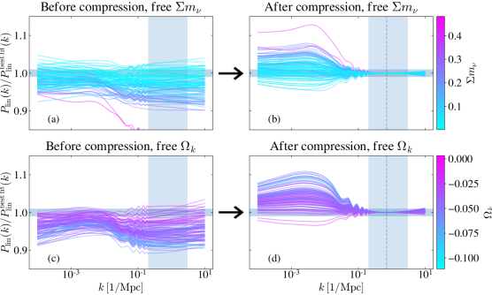
Figure 1 demonstrates why we consider just two parameters describing a slope and an amplitude to be sufficient to parameterise the linear matter power spectrum within this regime. In panel (a), we randomly sample 100 points from the Planck chains [43] with free $\Sigma m_{\nu}$, and plot the ratio of the linear matter power spectrum at $z=3$ with the baseline $\Lambda$CDM best fit model, which we denote as $P_{\mathrm{lin}}^{\mathrm{\,best\>fit}}$. The colour of each line indicates the neutrino mass value for each model. We see the expected behaviour where cosmologies with a higher neutrino mass tend to lead to a suppression of the power spectrum on small scales at late times. In panel (b), we take the same 100 samples and rescale the amplitude and slope of the power spectrum in order to match the small-scale linear power in $P_{\mathrm{lin}}^{\mathrm{\,best\>fit}}$ as parameterised by equations 2.1 and 2.2. The vertical shaded region shows the approximate length scales to which the $P_{\mathrm{1D}}$ is sensitive in BOSS data [22]. The upcoming DESI results will provide an improved measurement of the $P_{\mathrm{1D}}$ over the same range of wavenumbers, so the arguments presented in this paper will continue to apply. The horizontal band shows the region of $1\%$ agreement. The effects on the linear matter power spectrum of variations in the 7 free parameters are captured by changes to the slope and amplitude to within $1\%$ (and often much better) when considering only the length scales within the shaded region. This is compared with the most recent constraints on the amplitude of the small-scale linear power spectrum from BOSS which have an uncertainty of $6\%$ [5]. In the bottom panels (c) and (d) we repeat the procedure for a chain with free curvature parameter $\Omega_{k}$ instead of $\Sigma m_{\nu}$. Again we see that the all the variations in cosmology are degenerate with changing just the slope and amplitude of the power spectrum on the scales of interest.

A natural extension to $\Delta^{2}_{p}$ and $n_{p}$ would be to include a parameter describing the second order derivative in the linear power around $k_{p}$ (a running of the small-scale linear power spectrum). The necessity of this parameter would be determined by the variation in the running within the prior range of the cosmological models under investigation, and the $k$ range and precision of the observational dataset. It would also be possible to include an extra parameter describing the growth rate if deemed necessary. We leave such extensions to future work.

2.2 Intergalactic medium

The neutral hydrogen density is determined both by the density of hydrogen (dependent upon the clustering as described in the previous section, as well as the mean baryon density $\omega_{b}$) and the ionisation state, which is itself affected by several astrophysical factors. A primary factor is the intensity of the ionising metagalactic UV background (UVB), which is highly uncertain. Assuming ionisation equilibrium this is balanced with the rate of recombination, which is dependent on the gas temperature. We parameterise these effects in terms of an effective optical depth, $\tau_{\mathrm{eff}}$, which is related to the mean transmitted flux fraction $\langle F\rangle$ by $\tau_{\mathrm{eff}}=-\mathrm{ln}\langle F\rangle$.

The thermal state of the gas around the mean cosmic density regions that are probed by the Ly$\alpha$ forest is well approximated by a power-law:

$$T(\Delta_{b})=T_{0}\Delta_{b}^{\gamma-1},$$ (2.3)

where $\Delta_{b}=\rho_{b}/\bar{\rho}_{b}$ is the baryon overdensity , $T_{0}$ is the gas temperature in $\mathrm{K}$ at mean density [53] and $\gamma$ is a free parameter. The effect of $T_{0}$ on the recombination rate is captured by $\langle F\rangle$, however thermal motion of the gas particles also induces a Doppler broadening of the absorption features. This has the effect of smoothing the $P_{\mathrm{1D}}$ on small scales. We describe this with a thermal broadening scale

$$\sigma_{T}=9.1\sqrt{\frac{T_{0}}{10000}}\frac{1+z}{H(z)},$$ (2.4)

where the factor $(1+z)/H(z)$ is required to convert the broadening scale from $\mathrm{km/s}$ to $\mathrm{Mpc}$ (to match the units in which we store the $P_{\mathrm{1D}}$). We include the parameters $\sigma_{T}$ and $\gamma$ in order to characterise the effects of gas temperature on the $P_{\mathrm{1D}}$.

On small scales the baryons are supported by gas pressure, leading to a small-scale suppression in the baryon power spectrum which therefore affects the Ly$\alpha$ forest. Unlike the thermal broadening, this is a 3D effect that also affects correlations perpendicular to the line of sight. Following ref. [54] we parameterise this effect with a pressure smoothing scale, $k_{F}$, in units of $\mathrm{Mpc}^{-1}$.

3 Simulations

To create a set of training data for constructing the emulator we present in section 4, we run a suite of 30 hydrodynamical simulations using the TreeSPH code MP-Gadget [55], a variant of the widely used Gadget-2 [56] with improved parallelisation and gravitational force solver. The speed of these simulations is increased using the QuickLymanAlpha option which turns regions of baryon overdensity exceeding $10^{3}$ and with temperatures $T<10^{5}$ K into stars. These highly non-linear regions are computationally expensive to evolve but do not contribute to the Ly$\alpha$ forest [26]. Our simulation box size is $L=67.5$ Mpc with $768^{3}$ CDM and baryon particles. These values were chosen as a compromise between modelling the low $k_{\parallel}$ modes that play an important role in cosmological constraints from BOSS data, and modelling the small-scale effects of pressure smoothing of the IGM within computational constraints.

The simulations start at $z=99$ from initial conditions created using MP-GenIC, which computes initial displacements using the Zel’dovich approximation. The baryons and dark matter are initialised on an offset grid using species-specific transfer functions calculated in CLASS [57]. Following the simulations presented in ref. [58], in order to reduce the effects of cosmic variance we adopt the ‘paired-and-fixed’ approach from refs. [59, 60, 61]. In this method, the initial amplitudes of the Fourier modes are fixed, with random phases. The same random seed is used for all simulations, meaning that the residual cosmic variance after applying the paired-fixed approach is the same in each simulation. We do not include any modelling of AGN feedback. We output snapshots at $4>z>2$ at intervals of $\Delta z=0.25$. Note that this redshift information is not included in the emulator. For each simulation snapshot we calculate the transmitted flux fraction along $500^{2}$ lines of sight using the postprocessing code “fake_spectra” [62]. We take the Fourier transform of the flux fraction along each line of sight, and find the average of each Fourier mode to calculate the $P_{\mathrm{1D}}$. The line-of-sight resolution is set to $0.05\,\mathrm{Mpc}$, which is high enough to resolve the thermal broadening scale $\sigma_{T}$ whose distribution is shown in figure 2. Box sizes and flux line-of-sight resolutions are chosen such that our mock $P_{\mathrm{1D}}$ have the same spacing in $k_{\parallel}$ for all simulations and snapshots.

	Training simulations	central sim	$h$ sim	$\nu$ sim
$A_{s}(\times 10^{-9})$	$[1.35\mbox{--}2.71]$	2.00	2.01	2.25
$n_{s}$	$[0.92\mbox{--}1.02]$	0.97	0.97	0.97
$h$	0.67	0.67	0.74	0.67
$\Omega_{m}$	0.316	0.316	0.259	0.324
$\Sigma m_{\nu}$ (eV)	0.0	0.0	0.0	0.3
$\Delta^{2}_{p}(z=3)$	$[0.25$–$0.45]$	0.35
$n_{p}(z=3)$	$-[2.35\mbox{--}2.25]$	$-2.30$
$z_{\mathrm{rei}}$	$[5.5\mbox{--}15]$	10.5
$H_{A}$	$[0.5\mbox{--}1.5]$	1.0
$H_{S}$	$[0.5\mbox{--}1.5]$	1.0

Table 1: Cosmological and astrophysical parameters for the training and test simulations. The limits of the Latin hypercube for the training simulations are shown in the left column, where only the primordial power spectrum and astrophysical parameters are varied. The primordial parameters $A_{s}$ and $n_{s}$ here are defined at the CMB pivot scale of $k=0.05\>\mathrm{Mpc}^{-1}$. The central sim, $h$ sim and $\nu$ sim test simulations are constructed such that they have the same small scale linear matter power spectrum ($\Delta^{2}_{p}$ and $n_{p}$) at $z=3$. For all simulations, we fix $\omega_{c}=0.12$, $\omega_{b}=0.022$.

In order to ensure that our training data are well distributed within the range of physically interesting models, the suite was set up using a Latin hypercube. The Latin hypercube spans the parameters $[\Delta^{2}_{p}(z=3),n_{p}(z=3),z_{\mathrm{rei}},H_{A},H_{S}]$, with the ranges shown in the left column of table 1. We use a flat $\Lambda$CDM cosmology, and vary only the primordial power spectrum in order to sample $\Delta^{2}_{p}$ and $n_{p}$. This will allow us to test later our hypotheses from section 2. We fix $\omega_{c}=0.12$, $\omega_{b}=0.022$ throughout this paper, since they are very well constrained by the CMB and otherwise poorly constrained by the Ly$\alpha$ forest. We also explore a range of IGM histories so that the astrophysical parameters in section 2.2 are well sampled. This is done using modifications [63] around a fiducial reionisation model presented in ref. [64], using a spatially uniform UVB. We define $z_{\mathrm{rei}}$ as the midpoint of HI reionisation, i.e. when the ionisation fraction of HI is 0.5, and modify the UVB rates such that this point ranges between $z_{\mathrm{rei}}\in[5.5,15]$. Following ref. [65], the thermal history is varied using parameters $H_{A}$ and $H_{S}$, which respectively rescale the amplitude of the gas heating rates, and the slope of their density dependence, $\epsilon=H_{A}\,\epsilon_{0}\,\Delta_{b}^{H_{S}}$. These translate most directly into changes to $T_{0}$ (and therefore $\sigma_{T}$) and $\gamma$ respectively.

In addition to the training simulations, we run three more simulations that we use for various tests, shown in the right side of table 1. The first is a simulation at the centre of the Latin hypercube of simulation parameters in table 1. We refer to this as the central sim. Second we run a $\Lambda$CDM simulation with a different background expansion and growth, labelled $h$ sim, with a larger value of $h=0.74$ at fixed physical densities ($\omega_{c}$, $\omega_{b}$). Finally we run a simulation with $0.3\,\mathrm{eV}$ massive neutrinos, labelled $\nu$ sim, where the neutrinos are implemented using the linear response approximation from ref. [66]. Again we keep $\omega_{c}$ and $\omega_{b}$ fixed. The values of $A_{s}$ in these test simulations are all set such that $\Delta^{2}_{p}(z=3)=0.35$, which is the midpoint of the Latin hypercube of the training data. We use the same reionisation model in all test simulations. These simulations are therefore constructed in such a way that they lie in the same central part of emulator parameter space. In the case of the $\nu$ sim, this leads to an increase in $A_{s}$ to compensate for the suppression of the linear power on small scales caused by massive neutrino free streaming [58].

Figure 2: Distribution of the 270 training points in three example 2D projections. We colour training points by redshift purely for illustration, since we do not include redshift information in our emulator. The $z=3$ training points are highlighted in red for use in figure 4. The Latin hypercube in simulation parameters shown in table 1 does not propagate into a Latin hypercube in emulator parameters, but ensures that the physically interesting parts of parameter space are populated with training points.

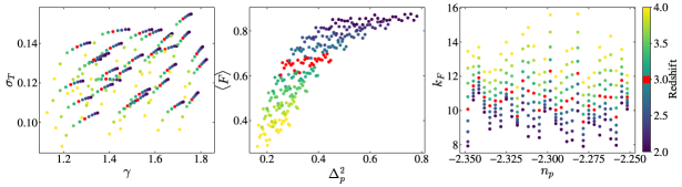
The 30 training simulations, each with 9 snapshots, produce a total of 270 mock $P_{\mathrm{1D}}$ measurements. The Latin hypercube of simulation parameters in table 1 does not propagate into a Latin hypercube in the parameters described in section 2, but it does ensure that the physically motivated regions of this parameter space are well populated with training points. In figure 2 we show the distribution of these training points in three projections of our six dimensional emulator parameter space. The points are coloured corresponding to the redshift of each training point, although we show this purely for illustrative purposes. We assume that these 6 parameters are sufficient to describe the $P_{\mathrm{1D}}$ without including explicit redshift information, and so we construct a single training set combining points from all redshifts. We highlight training points at $z=3$ in red for discussion in section 4.

The trajectories of individual simulations can be identified most clearly in the left panel which shows the thermal parameters $\sigma_{T}$ and $\gamma$. The middle panel shows points in the $\langle F\rangle-\Delta^{2}_{p}$ plane. Both of these parameters are strongly correlated with redshift, and so large parts of this plane are unphysical, and therefore not populated with training points. Although we do not explicitly include redshift information in the emulator, we observe the redshift evolution of $P_{\mathrm{1D}}$ through the evolution of $\Delta^{2}_{p}$ and $\langle F\rangle$. In the right panel we show the distribution of training points in $k_{F}$ and $n_{p}$. There is no redshift evolution of $n_{p}$, and so once again the trajectories of individual simulations are identifiable. The pressure smoothing scale evolves monotonically with redshift as the gas accumulates thermal energy from the UV background.

4 Gaussian process emulator

The purpose of this paper is to model the $P_{\mathrm{1D}}$ as a function of the parameters described in section 2 using the simulations presented in section 3. To do this we use a Gaussian process (GP) [67] implemented in the Python package GPy [68]. Our simulations are constructed in such a way that every snapshot provides a measurement of the $P_{\mathrm{1D}}$ in 85 linearly spaced $k_{\parallel}$ bins covering the range $[0.0931<k_{\parallel}<7.91]\>\mathrm{Mpc}^{-1}$. Therefore we have a set of training points for each $k_{\parallel}$ bin, and we drop the $k_{\parallel}$ notation for the following discussion. We denote a point in parameter space as $\bm{\theta}=[\Delta^{2}_{p},n_{p},\langle F\rangle,\sigma_{T},\gamma,k_{F}]$. A GP models the function one wants to learn, in this case $P_{\mathrm{1D}}(\bm{\theta})$, as a collection of random variables that form a joint Gaussian distribution, i.e. $P_{\mathrm{1D}}(\bm{\theta})\sim\mathcal{N}(0,K(\bm{\theta},\bm{\theta}_{i}))$. Here $\bm{\theta}_{i}$ are the locations of the training points where we have modelled the $P_{\mathrm{1D}}$ using simulations, and $K(\bm{\theta},\bm{\theta}^{\prime})$ is a covariance kernel whose precise form will be discussed shortly. In order to approximate the Gaussian process prior of zero mean, we normalise the $P_{\mathrm{1D}}$ by the median value of the training data. At a test point $\bm{\theta}_{\star}$, the joint distribution of the test data $P_{\mathrm{1D}}(\bm{\theta_{\star}})$ and training data $P_{\mathrm{1D}}(\bm{\theta}_{i})$ can be written as

$$\begin{bmatrix}P_{\mathrm{1D}}(\bm{\theta}_{i})\\ P_{\mathrm{1D}}(\bm{\theta_{\star}})\end{bmatrix} \sim\mathcal{N}\bigg{(}0,\begin{bmatrix}K(\bm{\theta}_{i},\bm{\theta}_{i})+\sigma^{2}_{n}\mathbf{I}&K(\bm{\theta}_{i},\bm{\theta_{\star}})\\ K(\bm{\theta_{\star}},\bm{\theta}_{i})&K(\bm{\theta_{\star}},\bm{\theta_{\star}})\end{bmatrix}\bigg{)}$$ (4.1)

where $\sigma_{n}^{2}$ is a hyperparameter representing Gaussian noise on the training data. The mean and variance of the posterior predictive distribution given the training information at $\bm{\theta}_{i}$ are then taken as our estimates of the value and interpolation uncertainty for the $P_{\mathrm{1D}}(\bm{\theta_{\star}})$:

$$\mu=K(\bm{\theta_{\star}},\bm{\theta}_{i})[K(\bm{\theta}_{i},\bm{\theta}_{i})+\sigma^{2}_{n}\mathbf{I}]^{-1}P_{\mathrm{1D}}(\bm{\theta}_{i})$$ (4.2)

$$\sigma^{2}=K(\bm{\theta_{\star}},\bm{\theta_{\star}})-K(\bm{\theta_{\star}},\bm{\theta}_{i})[K(\bm{\theta}_{i},\bm{\theta}_{i})+\sigma^{2}_{n}\mathbf{I}]^{-1}K(\bm{\theta}_{i},\bm{\theta_{\star}}).$$ (4.3)

There is significant freedom in the choice of covariance kernel, which represents a weak prior on the behaviour of the underlying function one wants to model. We use a squared exponential kernel, also known as a radial basis function

$$K(\bm{\theta},\bm{\theta}^{\prime})=\sigma_{0}^{2}\mathrm{exp}\bigg{(}-\sum_{j}\frac{(\theta_{j}-\theta_{j}^{\prime})^{2}}{2l_{j}^{2}}\bigg{)},$$ (4.4)

with an independent correlation length $l_{i}$ in each parameter direction. It follows that our GP has a total of 8 hyperparameters: 6 correlation lengths, $\sigma_{0}^{2}$ and $\sigma_{n}^{2}$. The hyperparameters are optimised by maximising the marginal log likelihood of the training data [67]. This is done across all $k_{\parallel}$ bins simultaneously, so we use the same set of hyperparameters for the full bandpower description of the $P_{\mathrm{1D}}$. To avoid numerical issues, all of our parameters $\bm{\theta}$ are rescaled to vary within a unit volume before being passed to the emulator.

We briefly highlight the differences in this setup compared to previous applications of GPs to emulation of the $P_{\mathrm{1D}}$ [39, 40, 20]. These emulators trained an independent GP on each redshift bin, whereas we combine training points from all redshifts in one GP. These works also used a different covariance kernel, combining the squared exponential in equation 4.4 with a linear term, and used an isotropic correlation length. The parameterisation used in these works was such that the $P_{\mathrm{1D}}$ varied by a similar order of magnitude within the prior volume in each parameter direction, meaning that an isotropic kernel performed well. A major difference in our setup is that the sensitivity of the $P_{\mathrm{1D}}$ to each parameter varies strongly. This is reflected in the optimised correlation lengths, which range from $0.47$ for $\langle F\rangle$ to $11.5$ for $n_{p}$. Since we combine all training points in a single emulator and we use larger simulations with more $k_{\parallel}$ bins, there is more information in the training set with which to optimise a larger number of hyperparameters in an anisotropic kernel.

4.1 Emulator validation

In this section we validate the emulator predictions on simulation data. In figure 3 we show the results of a leave-one-out validation test iterated across the full suite of 30 training simulations. We compare the $P_{\mathrm{1D}}$ in the nine snapshots of each validation simulation with the predicted $P_{\mathrm{1D}}$ from an emulator trained on the rest of the suite. The solid red lines and shaded red regions respectively show the mean and variance standard deviation of the percentage error on these 30 predictions. The black solid lines show the $\pm$ median $1-\sigma$ uncertainty on the predictions as estimated by the GP using equation 4.3, and the gray shaded area shows the region of $1\%$ error. We show the accuracy of the emulator predictions at different redshifts to compare it with the uncertainty on BOSS measurements of the $P_{\mathrm{1D}}$ from ref. [5], represented by blue shaded regions.

Figure 3: Results of a ‘leave-one-out’ validation test on the GP emulator. For each of the 30 training simulations, we train the GP on the snapshots from 29 simulations and compare the GP prediction with the truth in each of the nine snapshots of the remaining simulation. The solid red line and red shaded region respectively show the mean and standard deviation of the empirical error (prediction - truth) from the 30 validation tests. The black solid lines around zero show the $\pm$ median of the theoretical uncertainty on the emulator predictions (computed from equation 4.3). The gray shaded area shows the region of $1\%$ error. We show the performance of the emulator at several redshifts to compare it with the observational uncertainties from the latest analysis of BOSS/eBOSS data (blue shaded regions [5]). We expect that $P_{\mathrm{1D}}$ measurements from DESI will cover a similar range of wavenumbers, but the systematic contribution to the data covariance is currently difficult to predict.

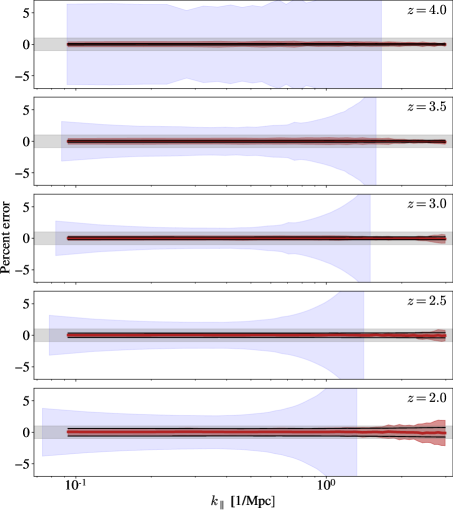
The emulator predictions are unbiased, with a mean error of $<1\%$ at the redshifts and wavenumbers measured by BOSS, eBOSS and DESI. The variance indicated by the shaded red region can be interpreted as an empirical estimate of the average error on emulator predictions. In all regimes probed by BOSS data this quantity is $<0.5\%$, considerably lower than observational uncertainties. The median theoretical error is slightly larger implying that emulator uncertainties are slightly overestimated, which was also the case in refs. [39, 40, 20]. Nevertheless, these uncertainties are still also well below those of the BOSS data. We do not include lines for DESI here as the exact increase in sensitivity is still uncertain. However it is worth noting that in the case where DESI errors become comparable to these uncertainties, there are several avenues to be explored such as changes to the covariance kernel to improve emulator performance or the addition of refinement simulations using Bayesian optimisation [40, 20].

Besides the measurements from BOSS and eBOSS, the Ly$\alpha$ forest $P_{\mathrm{1D}}$ has also been measured from small samples of very high-resolution spectra [17, 51, 69, 15, 16]. These measurements extend to higher redshift and smaller scales, and e.g. can be useful in breaking some of the parameter degeneracies (see appendix A). However, our simulations do not have the resolution required to resolve the pressure scale for some of the colder IGM models at $z>4$ (see right panel of figure 2).

4.2 Predictions at a redshift without training data

In constructing a single GP using training points from all redshifts, we are assuming that the $P_{\mathrm{1D}}$ is sufficiently well described by the six parameters from section 2, without the need to explicitly include redshift information in the emulator. Under this assumption, if one were to construct two simulations that had the same set of $\bm{\theta}$ parameters at different redshifts, the $P_{\mathrm{1D}}$ at these two different redshifts would be the same. In practice, engineering such a simulation is non-trivial due to the complex relationship between simulation parameters that model the IGM and the astrophysical emulator parameters. Therefore, in order to test this hypothesis, we construct an emulator dropping all training points at $z=3$ (the points shown in red in figure 2). We then use this emulator to predict the $P_{\mathrm{1D}}$ in the $z=3$ snapshots for 3 randomly chosen simulations, i.e. we are using training points at $z\leq 2.75$ and $3.25\leq z$ to predict the $P_{\mathrm{1D}}$ at $z=3$.

Figure 4: Emulator predictions for the $P_{\mathrm{1D}}$ at $z=3$ when using no $z=3$ training points. We leave the red points from figure 2 out of the training set and reoptimise the GP hyperparameters. The three panels show the error on the emulated $P_{\mathrm{1D}}$ for three randomly chosen simulations. The circles show the empirical error, and the coloured shaded region shows the $1-\sigma$ theoretical emulator uncertainty.

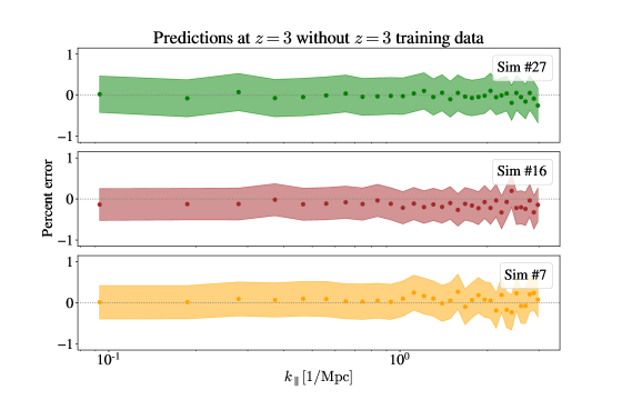
The accuracy of these predictions is shown in figure 4, with the theoretical uncertainty (computed using equation 4.3) on each prediction shown in the shaded coloured region. In each case the predictions have sub-percent accuracy over the full $k_{\parallel}$ range. This is a novel result that has not been possible with previous Ly$\alpha$ forest emulators, which validates our choice to combine training data from all redshifts and omit redshift information. The ability to emulate the $P_{\mathrm{1D}}$ at arbitrary redshifts also confers several advantages. In particular, our emulator could be used to analyse DESI measurements of $P_{\mathrm{1D}}$, regardless of the particular redshift binning of the data, which is currently unknown. Additionally, it is possible to combine training data from simulation suites with different output redshifts, making the construction of training sets more flexible.

4.3 Predicting extended models

Finally, we verify the emulator predictions on two test simulations: the $h$ sim and $\nu$ sim. The suite of training simulations has a fixed expansion history and growth rate, with only the primordial power spectrum varied in order to sample $\Delta^{2}_{p}$ and $n_{p}$. By fixing the growth rate in all training simulations, the emulator is learning the transfer function between the linear matter power spectrum and the $P_{\mathrm{1D}}$ for a fixed relationship between the density power spectrum and the velocity power spectrum. The velocity power spectrum will affect the $P_{\mathrm{1D}}$ through redshift space distortions (RSDs). Therefore it is important to test the accuracy of the emulator predictions in cosmologies with different growth rates to the training set. This will act as a test of our hypothesis that the $P_{\mathrm{1D}}$ is sensitive primarily to the linear matter power spectrum and insensitive to minor changes in the background expansion.

Figure 5: Accuracy of emulator predictions when tested on two test simulations from table 1. We test the emulator on different cosmological models to the training set, in which only the primordial power spectrum was varied. The red solid line shows the empirical accuracy of the emulator predictions, and the theoretical emulator uncertainty from equation 4.3 is shown in the red shaded region. In the left panel we show predictions for the $h$ sim, with $h=0.74$, where we have trained the emulator only on simulations with $h=0.67$. In the right panel, we show the accuracy of predictions for the $\nu$ sim which includes $\Sigma m_{\nu}=0.3\>\mathrm{eV}$ massive neutrinos. The vertical dotted line shows the highest $k_{\parallel}$ bin of BOSS data, and the horizontal gray band shows the region of $1\%$ error.

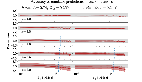
On the left side of figure 5, we show the accuracy of the emulated $P_{\mathrm{1D}}$ when compared with the truth in the $h$ sim. The vertical dotted line shows the highest wavenumbers in BOSS measurements [5], and the gray shaded area shows the region of $1\%$ accuracy. One way to consider this difference in $h$ within flat cosmologies is as a variation in the onset of dark energy. We are therefore changing the growth factor in the redshift range $4>z>2$, which will have two clear effects. First, the redshift evolution of $\Delta^{2}_{p}$ will change, and this effect is captured by our parameterisation. Second, the velocity power spectrum and therefore the RSDs will be different to the simulations in the training set. We are interested in determining whether this effect, which is not captured by any of our parameters, will impact the accuracy of the emulator predictions to a statistically-significant degree. Similarly to the tests shown in figure 3, the predictions have sub-percent accuracy in the regime probed by BOSS and DESI data. Therefore we can conclude that the effect on the growth rate for this scale of change in $h$ is negligible.

In ref. [58] it was shown that the effects of massive neutrinos on the $P_{\mathrm{1D}}$ are degenerate with changes to the amplitude of the linear power spectrum to within $1\%$. In that work it was difficult to disentangle effects of massive neutrinos on the IGM, that were partially accounted for by changing $\langle F\rangle$ and $\sigma_{T}$ in postprocessing. The emulator presented in this paper allows for this degeneracy to be tested more clearly since the effects of variations in the IGM and linear power spectrum can be predicted independently. The right side of figure 5 shows the accuracy of predictions compared with the truth in the $\nu$ sim, which has $\Sigma m_{\nu}=0.3\>\mathrm{eV}$. When adding massive neutrinos, we have kept $\omega_{b}$ and $\omega_{c}$ fixed. Therefore we are modifying the late-time growth and expansion rate governed by $\Omega_{m}$, which will have similar effects to the previous case on the IGM, the growth of structure, and baryon velocities. Another effect is the suppression of late-time, small-scale clustering due to free-streaming. This suppression is fairly large - approximately $8\%$ in the case of $\Sigma m_{\nu}=0.3\>\mathrm{eV}$, and it is this suppression that makes the Ly$\alpha$ forest a valuable probe of neutrino mass. Again the effect on the amplitude of clustering is captured in our setup by changes to $\Delta^{2}_{p}$. We see similar results to the previous test, in that the emulator predictions are accurate to less than 1 %, with the best performance at high $z$. Note that this neutrino mass is larger than current bounds $\Sigma m_{\nu}<0.12$ ($95\%$ credibility) from Planck + baryon acoustic oscillations (BAO) [43]. In this extreme case the emulator still performs well; the methodological errors for smaller neutrino masses will be even smaller. These results demonstrate that the relationship between the linear matter power spectrum and the $P_{\mathrm{1D}}$ is insensitive to the specific background expansion used in training the emulator. The test simulations were set up such that each emulator parameter is the same in both simulations to within $2\%$. This choice was made so that the accuracy of the predictions shown in figure 5 serves as a test of our parameterisation rather than as a test of the interpolation.

5 Parameter constraints

The ability of Ly$\alpha$ forest information alone to constrain cosmological parameters is limited by parameter degeneracies and insensitivities. The constraining power of the $P_{\mathrm{1D}}$ on cosmological parameters comes when combined with CMB information, and we leave a discussion on this for future work. However, in order to test the robustness of our emulator, we present parameter constraints from a Ly$\alpha$ forest-only likelihood on the amplitude and slope of the primordial power spectrum, $A_{s}$ and $n_{s}$ when using simulated mock data. In order to minimise degeneracies, these quantities are defined at a scale $k=0.7\>\mathrm{Mpc}^{-1}$. To further test the assumptions of fixing the growth and expansion rate, we also explore the sensitivity of the $P_{\mathrm{1D}}$ to $H_{0}$. Finally, we show constraints on $\Sigma m_{\nu}$ in order to investigate the degeneracy between $\Sigma m_{\nu}$ and $A_{s}$ [42, 58]. Given that constraints on $\Sigma m_{\nu}$ are a major motivation in $P_{\mathrm{1D}}$ analysis, understanding this degeneracy will be important in the analysis of DESI data.

5.1 Likelihood parameters

Given that our emulator parameters are not associated with any redshift, we do not attempt to constrain the emulator parameters themselves. For our likelihood parameter vector $\bm{\tilde{\theta}}$ we consider two classes of parameters – cosmological and IGM parameters. In section 5.3 the cosmological parameters we vary are $A_{s}$ and $n_{s}$, and we use uniform priors covering the ranges $[1.1,2.5]\times 10^{-9}$ and $[0.89,1.05]$ respectively. In section 5.4 we also vary $\Sigma m_{\nu}$ and $H_{0}$, with uniform priors covering the ranges $[0,1]\,\mathrm{eV}$ and $[55,90]\>\mathrm{km}\>\mathrm{s}^{-1}\>\mathrm{Mpc}^{-1}$ respectively. We keep the physical baryon and cold dark matter densities, $\omega_{c}$ and $\omega_{b}$, fixed to the values set in section 3. For each combination of these parameters we use CAMB to calculate the linear matter power spectra at each redshift where we have data, and we compute the corresponding values of $\Delta^{2}_{p}(z)$ and $n_{p}(z)$. Therefore each likelihood evaluation results in nine calls to the emulator.

To model the redshift evolution of the IGM parameters we use the redshift evolution of each parameter in the central sim described in table 1 as a fiducial model. The evolution of the IGM for this simulation and all 30 training simulations is shown in appendix B. To vary the IGM, we use a multiplicative rescaling $m(z)$ of this fiducial model using a power law around a pivot redshift:

$$\mathrm{ln}\,m(z)=X_{0}+X_{1}\mathrm{ln}\,\frac{1+z}{1+z_{\star}},$$ (5.1)

where we set $z_{\star}=3$ as it is the midpoint of our redshift outputs. $X_{0}$ controls the amplitude of the rescaling, and $X_{1}$ accommodates changes in the redshift evolution of a given parameter. The same approach is used for all IGM parameters, meaning we have a total of eight free parameters to model variations in the IGM. This model will not perfectly describe the evolution of the IGM in any simulation except the central sim and so we are not interested in constraints on these parameters per se, but instead interested in ensuring that we allow for enough variation in the IGM for a thorough marginalisation. The prior range for each parameter is $\in[-0.4,0.4]$, and we have verified that marginalised constraints on cosmological parameters are not impacted by expanding this range.

An advantage of omitting redshift information from the emulator is the increased flexibility in modelling the redshift evolution of the IGM. Since our emulator parameters are decoupled from simulation and likelihood parameters, the redshift dependence of the IGM is not fixed at the point of running the simulations as is the case in many previous setups. Whilst we use equation 5.1 to vary the IGM in this analysis, in principle any form of redshift evolution can be chosen provided it does not involve calls to the emulator that lie outside the convex hull of the training set.

Our baseline likelihood parameter vector is therefore

$$\bm{\tilde{\theta}}=[A_{s},n_{s},\mathrm{ln}\,\tau_{0},\mathrm{ln}\,\tau_{1},\mathrm{ln}\,\sigma_{0}^{T},\mathrm{ln}\,\sigma_{1}^{T},\mathrm{ln}\,\gamma_{0},\mathrm{ln}\,\gamma_{1},\mathrm{ln}\,k_{0}^{F},\mathrm{ln}\,k_{1}^{F}]$$ (5.2)

where $\tau_{i}$ represents rescalings to the effective optical depth, $\tau_{\mathrm{eff}}$, $\sigma^{T}_{i}$ to $\sigma_{T}$, $\gamma_{i}$ to $\gamma$, $k^{F}_{i}$ to $k_{F}$. The quantities that relate to physical length scales, $\sigma_{T}$ and $k_{F}$ are evaluated in velocity units.

5.2 Likelihood function

To more closely resemble a real analysis we perform our likelihood evaluations in velocity units. Since our emulator is constructed in comoving units, a cosmological model is required to convert between these using the relation $k=qH(z)/(1+z)$, where $k$ and $q$ are wavenumbers in comoving and velocity units respectively, and denote a flux power spectrum in velocity units as $\tilde{P}_{\mathrm{1D}}(q_{\parallel})$. We use the same $q_{\parallel}$ bins as the BOSS data [5], and use a cubic interpolation to rebin our mock and emulated flux power spectra to match the BOSS bins. We use a Gaussian likelihood function:

$$\mathrm{ln}\mathcal{L}(\bm{\tilde{\theta}})=\sum_{z}\bigg{[}-\frac{1}{2}\Delta_{i}(q_{i},z,\bm{\tilde{\theta}})C_{ij}(z,\bm{\tilde{\theta}})^{-1}\Delta_{j}(q_{j},z,\bm{\tilde{\theta}})-\frac{1}{2}\mathrm{log}\>\mathrm{det}\>C_{ij}(z,\bm{\tilde{\theta}})\bigg{]}$$ (5.3)

with

$$\Delta_{i}(q_{i},z,\bm{\tilde{\theta}})=\tilde{P}_{\mathrm{1D}}^{\mathrm{emu}}(q_{i},z,\bm{\tilde{\theta}})-\tilde{P}_{\mathrm{1D}}^{\mathrm{data}}(q_{i},z)$$ (5.4)

where $\tilde{P}_{\mathrm{1D}}^{\mathrm{emu}}(q_{i},z,\bm{\tilde{\theta}})$ is the theoretical prediction from the emulator for a given set of parameters $\bm{\tilde{\theta}}$, and $z$ is the redshift at which we are making the calls to the emulator. The covariance matrix $C_{ij}$ is a combination of the data and emulator covariance:

$$C_{\mathrm{ij}}(z,\bm{\tilde{\theta}})=C_{ij}^{\mathrm{data}}(z)+C_{ij}^{\mathrm{emu}}(z,\bm{\tilde{\theta}}).$$ (5.5)

In order to obtain results that resemble an analysis using current datasets, for the data covariance $C_{ij}^{\mathrm{data}}(z)$ we use the covariance matrices from the most recent measurement of the $\tilde{P}_{\mathrm{1D}}(q_{\parallel})$ from BOSS [5]. Our simulation snapshot outputs are different to the redshift binning of the BOSS measurements, so for each $z$ where we have mock data, we simply use the covariance matrix from the closest BOSS redshift bin, prioritising the lower $z$ bin in the case where the bins are equidistant. The emulator covariance matrix is constructed from the theoretical uncertainty on each emulator call, which is a function of the emulator hyperparameters and the local density of the training points. Given that both these properties are common to all $q$ bins, we assume the errors are maximally correlated and build $C_{ij}^{\mathrm{emu}}(z,\bm{\tilde{\theta}})$ under this assumption. Since we use the same random seed in all simulations, any residual cosmic variance that remains after applying the ‘paired-and-fixed’ approach is the same in all simulations. We do not add noise realisations to the mock data drawn from the mock data covariance. The likelihood function is sampled using MCMC sampling implemented in emcee [70], and we check for convergence of the integrated autocorrelation time.

5.3 MCMC results

Figure 6: Accuracy of marginalised constraints on $A_{s}$ and $n_{s}$ for each of the 30 training simulations, with $1-\sigma$ credible bounds.

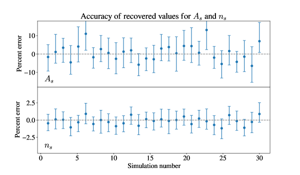
In figure 6 we show the accuracy of marginalised constraints on $A_{s}$ and $n_{s}$ for each of the 30 training simulations when running with 10 free parameters: $A_{s}$ and $n_{s}$ and the 8 IGM parameters described earlier. We fix $h$ and $\Sigma m_{\nu}$ to the true values of $h=0.67$ and $\Sigma m_{\nu}=0\,\mathrm{eV}$. As in section 4.1, for each constraint we leave the validation simulation out of the emulator training set. The error bars show the $1-\sigma$ uncertainty. In all but 3 cases we recover the correct cosmology to within $1-\sigma$.

5.4 Extended models

Figure 7: Marginalised 1D and 2D posterior distributions when using the $h$ sim as mock data. The true values are indicated by the dashed lines, with the contours showing the $68\%$ and $95\%$ credible regions. $A_{s}$ and $n_{s}$ are defined at a pivot scale of $k=0.7\>\mathrm{Mpc}^{-1}$. The shaded area of the 1D posteriors shows the $68\%$ credible region. Posteriors for the remaining parameters are shown in appendix C.

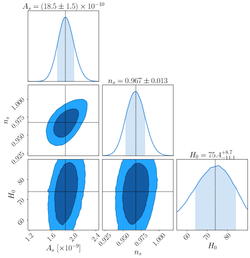
In figure 7 we show constraints on $A_{s}$, $n_{s}$ and $H_{0}$ after marginalising over the IGM parameters, using the $h$ sim as mock data. We set a wide prior range of $H_{0}\in[55,90]\>\mathrm{km}\>\mathrm{s}^{-1}\>\mathrm{Mpc}^{-1}$. Since the Ly$\alpha$ forest is observed in velocity units, our emulator predictions undergo a conversion from comoving to velocity units using the factor $H(z)/(1+z)$. Therefore we expect the constraints on the amplitude of the power spectrum to be degenerate with $H(z)$. This is evident in the lower left contour of figure 7. The degeneracy is weakened by the fact that we are probing a high redshift where the differences in $H(z)$ are smaller. For example, across the wide prior range, there is only a $6\%$ difference in $H(z=2)$, and a $1.5\%$ difference at $H(z=4)$. The constraints on $A_{s}$ and $n_{s}$ are accurate. This is an important demonstration, as we are correctly recovering parameters in a cosmology with a different background evolution to the one used in constructing the emulator.

Figure 8: Marginalised 1D and 2D posterior distributions when using the $\nu$ sim as mock data, with $\Sigma m_{\nu}$ as a free parameter. The true values are indicated by the dashed lines, with the contours showing the $68\%$ and $95\%$ credible regions. $A_{s}$ and $n_{s}$ are defined at a pivot scale of $k=0.7\>\mathrm{Mpc}^{-1}$. The shaded areas of the 1D posteriors show the $68\%$ credible region. For clarity in the figure, we do not show posteriors for the 8 free IGM parameters in this chain.

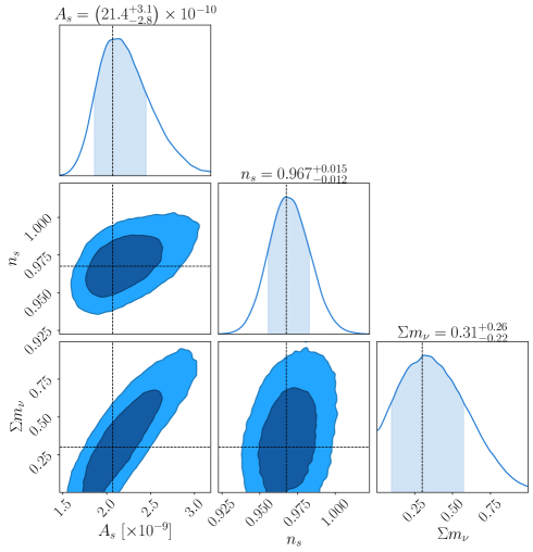
In figure 8 we show marginalised constraints when using the $\nu$ sim as mock data, allowing neutrino mass to vary in the range $\Sigma m_{\nu}\in[0.0,1.0]\,\mathrm{eV}$. The effects of massive neutrinos on cosmology are to vary both the expansion history and the growth rate, and to suppress the amplitude of matter clustering on small scales. Given the results of the previous figure, we expect the effects of massive neutrinos on the expansion and growth to have negligible contributions to the constraints. We use an extreme value of $\Sigma m_{\nu}=0.3\,\mathrm{eV}$ that is significantly higher than the current bound $\Sigma m_{\nu}<0.12\,\mathrm{eV}$ ($95\%$ credibility) from joint Planck + BAO data [43]. The neutrino mass is strongly degenerate with $A_{s}$ when using the Lya forest alone [42, 58]; stronger bounds arise from a combination with CMB data by breaking the degeneracy (e.g [31, 32]).

6 Discussion

We have presented a Gaussian process emulator that predicts the $P_{\mathrm{1D}}$ of the Ly$\alpha$ forest as a function of the amplitude and slope of the small-scale linear matter power spectrum and the state of the intergalactic medium. This work is an application of modern simulation interpolation techniques to a modelling approach that was more prevalent in early analysis of the Ly$\alpha$ forest, based on the fact that the cosmological information in the Ly$\alpha$ forest is concentrated in the linear matter power spectrum at the observed redshift. This is due to a unique property of the Ly$\alpha$ forest, in that it probes the universe at a period very close to an Einstein de-Sitter model. In this regime, variations in the $P_{\mathrm{1D}}$ due to differences in the growth rate and expansion history (allowed by current data) are negligible. For the first time we test the accuracy of this approximation at the level required by current datasets, and show that it holds. In particular, we showed that even in models with massive neutrinos, the cosmological information in $P_{\mathrm{1D}}$ analysis is contained in the slope and amplitude of the linear power spectrum within current observational uncertainty.

In addition to being lower dimensional in the cosmological sector, our emulator affords other practical advantages. By emulating the flux power spectrum independently of redshift, predictions can be made to sub-percent accuracy at redshifts not necessarily included in the training simulations. This affords flexibility with regards to the analysis of future data. Moreover, the redshift evolution of the IGM can be modelled at the point of constructing a likelihood function, as opposed to being determined at the point of constructing the emulator as in many previous frameworks.

Whilst we demonstrated that this emulator can be applied to massive neutrino cosmologies without massive neutrinos used in the training set, the same principle can be applied to a wider range of extended cosmological models, e.g. running of the spectral index in the primordial power spectrum or curved universes [43]. There are two conditions under which our implementation would not be valid. Models with sharp features in the small-scale matter power spectrum (such as warm dark matter models [71, 17] or ultra-light axion dark matter [46, 47]), or models with a non-standard relationship between the baryon density and velocities (such as modified gravity models [72]). However, simple extensions to the emulator parameter space could incorporate some of these models too (e.g. [38, 20]), and the motivations for parameterising the $P_{\mathrm{1D}}$ in terms of the linear power spectrum still apply.

The joint analysis of CMB observations with measurements of the small-scale linear matter power spectrum from the Ly$\alpha$ forest has long been a powerful combination in constraining extensions to $\Lambda$CDM [23, 24, 25, 27, 26, 28, 73, 74, 75]. We presented an emulator that will facilitate the combination of current (BOSS/eBOSS) and upcoming DESI measurements of the $P_{\mathrm{1D}}$ with CMB observations, to provide competitive constraints on beyond-$\Lambda$CDM cosmologies.

Appendix A Parameter dependence of the $P_{\mathrm{1D}}$

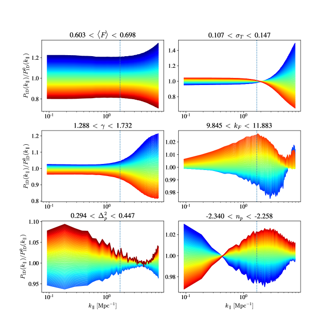
In figure 9 we use the GP presented in section 4 to show the fractional change of the $P_{\mathrm{1D}}$ in response to changes of each of the parameters described in section 2. We show the fractional change around a central point in parameter space set by the midpoint of all training points at $z=3$, i.e. the points shown in red in figure 2. We denote this point as $P_{\mathrm{1D}}^{0}(k_{\parallel})$. We show the change in the $P_{\mathrm{1D}}$ with respect to $P_{\mathrm{1D}}^{0}(k_{\parallel})$ when moving from edge to edge of the convex hull of the full training set, to ensure that we are not extrapolating into regions of parameter space where the GP cannot reliably predict the $P_{\mathrm{1D}}$. The blue dotted lines show the highest $k_{\parallel}$ probed by BOSS [5]. The effects of IGM parameters are most dominant at higher wavenumbers than those probed by BOSS data, with a degeneracy between $\langle F\rangle$ and $\gamma$ when looking only at the lower $k_{\parallel}$ modes.

Figure 9: Fractional effect on the $P_{\mathrm{1D}}$ of changing each of the six emulator parameters. We chose as a reference model, $P_{\mathrm{1D}}^{0}(k_{\parallel})$ the midpoint of the $z=3$ training points, and show the effect on the $P_{\mathrm{1D}}$ when moving from edge to edge of the convex hull of the training set. Lowest values for each parameter are coloured blue, transitioning to the highest values in red. The blue dotted line represents the highest $k_{\parallel}$ bin in BOSS data [5].

Appendix B IGM evolution

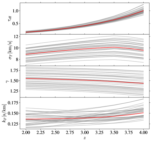
We plot the redshift evolution of each IGM parameter for all 30 training simulations in gray lines in figure 10, with the central simulation shown in red. The values in red are used to provide a fiducial model for the marginalisation over the IGM described in section 5. The mean flux, $\langle F\rangle$ is found by averaging over the flux transmission fraction in every line-of-sight pixel of a given snapshot. To calculate the thermal parameters, $\sigma_{T}$ and $\gamma$, the particle snapshot data is binned in the $\mathrm{log}_{10}T-\mathrm{log}_{10}\Delta_{b}$ plane, where $T$ is in units of $\mathrm{K}$. We then perform a linear fit to the mode within the range $-1.5<\mathrm{log}_{10}\Delta_{b}<0.5$ to obtain values for $T_{0}$ and $\gamma$ from equation 2.3. $T_{0}$ is then converted into a value for $\sigma_{T}$ using equation 2.4. In order to calculate the pressure smoothing scale, $k_{F}$, we follow the approach in ref. [54]. We calculate the real-space Lyman-$\alpha$ forest 3D flux power spectrum, $\Delta^{2}_{F}(k)$, and fit an exponential cutoff of the following form:

$$\Delta^{2}_{F}(k)=Ak^{n}\mathrm{exp}\bigg{(}-\frac{k^{2}}{k^{2}_{F}}\bigg{)},$$ (B.1)

where $A$ and $n$ are free parameters.

Figure 10: Redshift evolution of the IGM parameters for each of our 30 training simulations in gray. In red we show the IGM parameters for the central sim which is used as a fiducial model in section 5.

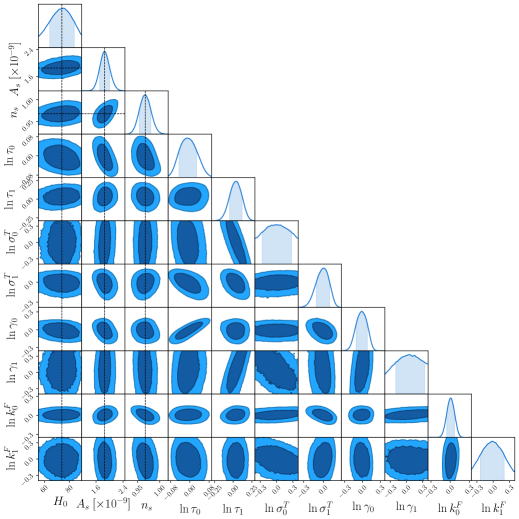
Appendix C Full posterior with IGM parameters

In section 5 we presented MCMC posteriors for several analyses on mock data, after marginalising over the 8 IGM parameters. In figure 11 we show the full posterior for one of the analyses, including cosmological and IGM parameters.

Figure 11: Marginalised 1D and 2D posterior distributions for all free parameters when using the $h$ sim as mock data (the same as in figure 7).

References

- [1] K. S. Dawson, D. J. Schlegel, C. P. Ahn, S. F. Anderson, É. Aubourg, S. Bailey et al., The Baryon Oscillation Spectroscopic Survey of SDSS-III, AJ 145 (2013) 10 [1208.0022].
- [2] K. S. Dawson, J.-P. Kneib, W. J. Percival, S. Alam, F. D. Albareti, S. F. Anderson et al., The SDSS-IV Extended Baryon Oscillation Spectroscopic Survey: Overview and Early Data, AJ 151 (2016) 44 [1508.04473].
- [3] H. du Mas des Bourboux, J. Rich, A. Font-Ribera, V. de Sainte Agathe, J. Farr, T. Etourneau et al., The Completed SDSS-IV extended Baryon Oscillation Spectroscopic Survey: Baryon acoustic oscillations with Lyman- forests, arXiv e-prints (2020) arXiv:2007.08995 [2007.08995].
- [4] N. Palanque-Delabrouille, C. Yèche, A. Borde, J.-M. Le Goff, G. Rossi, M. Viel et al., The one-dimensional Ly forest power spectrum from BOSS, Astron. Astrophys. 559 (2013) A85 [1306.5896].
- [5] S. Chabanier, N. Palanque-Delabrouille, C. Yèche, J.-M. Le Goff, E. Armengaud, J. Bautista et al., The one-dimensional power spectrum from the SDSS DR14 Ly forests, JCAP 2019 (2019) 017 [1812.03554].
- [6] DESI Collaboration, A. Aghamousa, J. Aguilar, S. Ahlen, S. Alam, L. E. Allen et al., The DESI Experiment Part I: Science,Targeting, and Survey Design, arXiv e-prints (2016) arXiv:1611.00036 [1611.00036].
- [7] R. A. C. Croft, D. H. Weinberg, N. Katz and L. Hernquist, Recovery of the Power Spectrum of Mass Fluctuations from Observations of the Ly Forest, ApJ 495 (1998) 44 [astro-ph/9708018].
- [8] R. A. C. Croft, D. H. Weinberg, M. Pettini, L. Hernquist and N. Katz, The Power Spectrum of Mass Fluctuations Measured from the Ly Forest at Redshift z = 2.5, ApJ 520 (1999) 1 [astro-ph/9809401].
- [9] P. McDonald, J. Miralda-Escudé, M. Rauch, W. L. W. Sargent, T. A. Barlow, R. Cen et al., The Observed Probability Distribution Function, Power Spectrum, and Correlation Function of the Transmitted Flux in the Ly Forest, ApJ 543 (2000) 1 [astro-ph/9911196].
- [10] N. Y. Gnedin and A. J. S. Hamilton, Matter power spectrum from the Lyman-alpha forest: myth or reality?, Mon. Not. Roy. Astron. Soc. 334 (2002) 107 [astro-ph/0111194].
- [11] R. A. C. Croft, D. H. Weinberg, M. Bolte, S. Burles, L. Hernquist, N. Katz et al., Toward a Precise Measurement of Matter Clustering: Ly Forest Data at Redshifts 2-4, ApJ 581 (2002) 20 [astro-ph/0012324].
- [12] M. Viel, M. G. Haehnelt and V. Springel, Inferring the dark matter power spectrum from the Lyman forest in high-resolution QSO absorption spectra, Mon. Not. Roy. Astron. Soc. 354 (2004) 684 [astro-ph/0404600].
- [13] P. McDonald, U. Seljak, R. Cen, D. Shih, D. H. Weinberg, S. Burles et al., The Linear Theory Power Spectrum from the Ly Forest in the Sloan Digital Sky Survey, ApJ 635 (2005) 761 [astro-ph/0407377].
- [14] J. Oñorbe, J. F. Hennawi, Z. Lukić and M. Walther, Constraining Reionization with the z 5-6 Ly Forest Power Spectrum: The Outlook after Planck, ApJ 847 (2017) 63 [1703.08633].
- [15] M. Walther, J. Oñorbe, J. F. Hennawi and Z. Lukić, New Constraints on IGM Thermal Evolution from the Ly Forest Power Spectrum, ApJ 872 (2019) 13 [1808.04367].
- [16] E. Boera, G. D. Becker, J. S. Bolton and F. Nasir, Revealing Reionization with the Thermal History of the Intergalactic Medium: New Constraints from the Ly Flux Power Spectrum, ApJ 872 (2019) 101 [1809.06980].
- [17] M. Viel, G. D. Becker, J. S. Bolton and M. G. Haehnelt, Warm dark matter as a solution to the small scale crisis: New constraints from high redshift Lyman- forest data, Phys. Rev. D 88 (2013) 043502 [1306.2314].
- [18] V. Iršič, M. Viel, M. G. Haehnelt, J. S. Bolton, S. Cristiani, G. D. Becker et al., New constraints on the free-streaming of warm dark matter from intermediate and small scale Lyman- forest data, Phys. Rev. D 96 (2017) 023522 [1702.01764].
- [19] V. Iršič, M. Viel, M. G. Haehnelt, J. S. Bolton and G. D. Becker, First Constraints on Fuzzy Dark Matter from Lyman- Forest Data and Hydrodynamical Simulations, Phys. Rev. L 119 (2017) 031302 [1703.04683].
- [20] K. K. Rogers and H. V. Peiris, General framework for cosmological dark matter bounds using -body simulations, arXiv e-prints (2020) arXiv:2007.13751 [2007.13751].
- [21] K. K. Rogers and H. V. Peiris, Strong bound on canonical ultra-light axion dark matter from the Lyman-alpha forest, arXiv e-prints (2020) arXiv:2007.12705 [2007.12705].
- [22] S. Chabanier, M. Millea and N. Palanque-Delabrouille, Matter power spectrum: from Ly forest to CMB scales, Mon. Not. Roy. Astron. Soc. 489 (2019) 2247 [1905.08103].
- [23] J. Phillips, D. H. Weinberg, R. A. C. Croft, L. Hernquist, N. Katz and M. Pettini, Constraints on Cosmological Parameters from the Ly Forest Power Spectrum and COBE DMR, ApJ 560 (2001) 15 [astro-ph/0001089].
- [24] L. Verde, H. V. Peiris, D. N. Spergel, M. R. Nolta, C. L. Bennett, M. Halpern et al., First-Year Wilkinson Microwave Anisotropy Probe (WMAP) Observations: Parameter Estimation Methodology, ApJS 148 (2003) 195 [astro-ph/0302218].
- [25] D. N. Spergel, L. Verde, H. V. Peiris, E. Komatsu, M. R. Nolta, C. L. Bennett et al., First-Year Wilkinson Microwave Anisotropy Probe (WMAP) Observations: Determination of Cosmological Parameters, ApJS 148 (2003) 175 [astro-ph/0302209].
- [26] M. Viel, J. Weller and M. G. Haehnelt, Constraints on the primordial power spectrum from high-resolution Lyman forest spectra and WMAP, Mon. Not. Roy. Astron. Soc. 355 (2004) L23 [astro-ph/0407294].
- [27] U. Seljak, A. Makarov, P. McDonald, S. F. Anderson, N. A. Bahcall, J. Brinkmann et al., Cosmological parameter analysis including SDSS Ly forest and galaxy bias: Constraints on the primordial spectrum of fluctuations, neutrino mass, and dark energy, Phys. Rev. D 71 (2005) 103515 [astro-ph/0407372].
- [28] U. Seljak, A. Slosar and P. McDonald, Cosmological parameters from combining the Lyman- forest with CMB, galaxy clustering and SN constraints, JCAP 2006 (2006) 014 [astro-ph/0604335].
- [29] S. Bird, H. V. Peiris, M. Viel and L. Verde, Minimally parametric power spectrum reconstruction from the Lyman forest, Mon. Not. Roy. Astron. Soc. 413 (2011) 1717 [1010.1519].
- [30] N. Palanque-Delabrouille, C. Yèche, J. Lesgourgues, G. Rossi, A. Borde, M. Viel et al., Constraint on neutrino masses from SDSS-III/BOSS Ly forest and other cosmological probes, Journal of Cosmology and Astro-Particle Physics 2015 (2015) 045 [1410.7244].
- [31] N. Palanque-Delabrouille, C. Yèche, J. Baur, C. Magneville, G. Rossi, J. Lesgourgues et al., Neutrino masses and cosmology with Lyman-alpha forest power spectrum, JCAP 2015 (2015) 011 [1506.05976].
- [32] N. Palanque-Delabrouille, C. Yèche, N. Schöneberg, J. Lesgourgues, M. Walther, S. Chabanier et al., Hints, neutrino bounds, and WDM constraints from SDSS DR14 Lyman- and Planck full-survey data, JCAP 2020 (2020) 038 [1911.09073].
- [33] M. McQuinn, The Evolution of the Intergalactic Medium, Ann. Rev. Astron. & Astrophys. 54 (2016) 313 [1512.00086].
- [34] J. Kwan, K. Heitmann, S. Habib, N. Padmanabhan, E. Lawrence, H. Finkel et al., Cosmic Emulation: Fast Predictions for the Galaxy Power Spectrum, ApJ 810 (2015) 35 [1311.6444].
- [35] Z. Zhai, J. L. Tinker, M. R. Becker, J. DeRose, Y.-Y. Mao, T. McClintock et al., The Aemulus Project. III. Emulation of the Galaxy Correlation Function, ApJ 874 (2019) 95 [1804.05867].
- [36] M. Viel and M. G. Haehnelt, Cosmological and astrophysical parameters from the Sloan Digital Sky Survey flux power spectrum and hydrodynamical simulations of the Lyman forest, Mon. Not. Roy. Astron. Soc. 365 (2006) 231 [astro-ph/0508177].
- [37] A. Borde, N. Palanque-Delabrouille, G. Rossi, M. Viel, J. S. Bolton, C. Yèche et al., New approach for precise computation of Lyman- forest power spectrum with hydrodynamical simulations, Journal of Cosmology and Astro-Particle Physics 2014 (2014) 005 [1401.6472].
- [38] R. Murgia, V. Iršič and M. Viel, Novel constraints on noncold, nonthermal dark matter from Lyman- forest data, Phys. Rev. D 98 (2018) 083540 [1806.08371].
- [39] S. Bird, K. K. Rogers, H. V. Peiris, L. Verde, A. Font-Ribera and A. Pontzen, An emulator for the Lyman- forest, JCAP 2019 (2019) 050 [1812.04654].
- [40] K. K. Rogers, H. V. Peiris, A. Pontzen, S. Bird, L. Verde and A. Font-Ribera, Bayesian emulator optimisation for cosmology: application to the Lyman-alpha forest, JCAP 2019 (2019) 031 [1812.04631].
- [41] T. Takhtaganov, Z. Lukic, J. Mueller and D. Morozov, Cosmic Inference: Constraining Parameters With Observations and Highly Limited Number of Simulations, arXiv e-prints (2019) arXiv:1905.07410 [1905.07410].
- [42] M. Viel, M. G. Haehnelt and V. Springel, The effect of neutrinos on the matter distribution as probed by the intergalactic medium, JCAP 2010 (2010) 015 [1003.2422].
- [43] Planck Collaboration, N. Aghanim, Y. Akrami, M. Ashdown, J. Aumont, C. Baccigalupi et al., Planck 2018 results. VI. Cosmological parameters, Astron. Astrophys. 641 (2020) A6 [1807.06209].
- [44] J. Lesgourgues and S. Pastor, Massive neutrinos and cosmology, Phys. Rept. 429 (2006) 307 [astro-ph/0603494].
- [45] J. Lesgourgues and S. Pastor, Neutrino cosmology and Planck, New Journal of Physics 16 (2014) 065002 [1404.1740].
- [46] W. Hu, R. Barkana and A. Gruzinov, Fuzzy Cold Dark Matter: The Wave Properties of Ultralight Particles, Phys. Rev. L 85 (2000) 1158 [astro-ph/0003365].
- [47] L. Hui, J. P. Ostriker, S. Tremaine and E. Witten, Ultralight scalars as cosmological dark matter, Phys. Rev. D 95 (2017) 043541 [1610.08297].
- [48] M. Vogelsberger, J. Zavala, F.-Y. Cyr-Racine, C. Pfrommer, T. Bringmann and K. Sigurdson, ETHOS - an effective theory of structure formation: dark matter physics as a possible explanation of the small-scale CDM problems, Mon. Not. Roy. Astron. Soc. 460 (2016) 1399 [1512.05349].
- [49] J. König, A. Merle and M. Totzauer, keV sterile neutrino dark matter from singlet scalar decays: the most general case, JCAP 2016 (2016) 038 [1609.01289].
- [50] R. Adhikari, M. Agostini, N. A. Ky, T. Araki, M. Archidiacono, M. Bahr et al., A White Paper on keV sterile neutrino Dark Matter, JCAP 2017 (2017) 025 [1602.04816].
- [51] V. Iršič, M. Viel, T. A. M. Berg, V. D’Odorico, M. G. Haehnelt, S. Cristiani et al., The Lyman forest power spectrum from the XQ-100 Legacy Survey, Mon. Not. Roy. Astron. Soc. 466 (2017) 4332 [1702.01761].
- [52] A. G. Riess, L. M. Macri, S. L. Hoffmann, D. Scolnic, S. Casertano, A. V. Filippenko et al., A 2.4% Determination of the Local Value of the Hubble Constant, ApJ 826 (2016) 56 [1604.01424].
- [53] Z. Lukić, C. W. Stark, P. Nugent, M. White, A. A. Meiksin and A. Almgren, The Lyman forest in optically thin hydrodynamical simulations, Mon. Not. Roy. Astron. Soc. 446 (2015) 3697 [1406.6361].
- [54] G. Kulkarni, J. F. Hennawi, J. Oñorbe, A. Rorai and V. Springel, Characterizing the Pressure Smoothing Scale of the Intergalactic Medium, ApJ 812 (2015) 30 [1504.00366].
- [55] Y. Feng, S. Bird, L. Anderson, A. Font-Ribera and C. Pedersen, Mp-gadget/mp-gadget: A tag for getting a doi, Oct., 2018. 10.5281/zenodo.1451799.
- [56] V. Springel, The cosmological simulation code GADGET-2, Mon. Not. Roy. Astron. Soc. 364 (2005) 1105 [astro-ph/0505010].
- [57] J. Lesgourgues, The Cosmic Linear Anisotropy Solving System (CLASS) I: Overview, arXiv e-prints (2011) arXiv:1104.2932 [1104.2932].
- [58] C. Pedersen, A. Font-Ribera, T. D. Kitching, P. McDonald, S. Bird, A. Slosar et al., Massive neutrinos and degeneracies in Lyman-alpha forest simulations, JCAP 2020 (2020) 025 [1911.09596].
- [59] R. E. Angulo and A. Pontzen, Cosmological N-body simulations with suppressed variance, Mon. Not. Roy. Astron. Soc. 462 (2016) L1 [1603.05253].
- [60] L. Anderson, A. Pontzen, A. Font-Ribera, F. Villaescusa-Navarro, K. K. Rogers and S. Genel, Cosmological Hydrodynamic Simulations with Suppressed Variance in the Lyman- Forest Power Spectrum, arXiv e-prints (2018) arXiv:1811.00043 [1811.00043].
- [61] F. Villaescusa-Navarro, S. Naess, S. Genel, A. Pontzen, B. Wandelt, L. Anderson et al., Statistical Properties of Paired Fixed Fields, ApJ 867 (2018) 137 [1806.01871].
- [62] S. Bird, “FSFE: Fake Spectra Flux Extractor.” Astrophysics Source Code Library, Oct., 2017.
- [63] J. Oñorbe, J. F. Hennawi and Z. Lukić, Self-consistent Modeling of Reionization in Cosmological Hydrodynamical Simulations, ApJ 837 (2017) 106 [1607.04218].
- [64] F. Haardt and P. Madau, Radiative Transfer in a Clumpy Universe. IV. New Synthesis Models of the Cosmic UV/X-Ray Background, ApJ 746 (2012) 125 [1105.2039].
- [65] J. S. Bolton, M. Viel, T. S. Kim, M. G. Haehnelt and R. F. Carswell, Possible evidence for an inverted temperature-density relation in the intergalactic medium from the flux distribution of the Ly forest, Mon. Not. Roy. Astron. Soc. 386 (2008) 1131 [0711.2064].
- [66] Y. Ali-Haïmoud and S. Bird, An efficient implementation of massive neutrinos in non-linear structure formation simulations, Mon. Not. Roy. Astron. Soc. 428 (2013) 3375 [1209.0461].
- [67] C. E. Rasmussen and C. K. I. Williams, Gaussian Processes for Machine Learning. MIT Press, 2006.
- [68] GPy, “GPy: A gaussian process framework in python.” http://github.com/SheffieldML/GPy, since 2012.
- [69] C. Yèche, N. Palanque-Delabrouille, J. Baur and H. du Mas des Bourboux, Constraints on neutrino masses from Lyman-alpha forest power spectrum with BOSS and XQ-100, Journal of Cosmology and Astro-Particle Physics 2017 (2017) 047 [1702.03314].
- [70] D. Foreman-Mackey, D. W. Hogg, D. Lang and J. Goodman, emcee: The MCMC Hammer, Publications of the Astronomical Society of the Pacific 125 (2013) 306 [1202.3665].
- [71] M. Viel, J. Lesgourgues, M. G. Haehnelt, S. Matarrese and A. Riotto, Constraining warm dark matter candidates including sterile neutrinos and light gravitinos with WMAP and the Lyman- forest, Phys. Rev. D 71 (2005) 063534 [astro-ph/0501562].
- [72] M. Ishak, Testing general relativity in cosmology, Living Reviews in Relativity 22 (2019) 1 [1806.10122].
- [73] C. Dvorkin, K. Blum and M. Kamionkowski, Constraining dark matter-baryon scattering with linear cosmology, Phys. Rev. D 89 (2014) 023519 [1311.2937].
- [74] R. Krall, F.-Y. Cyr-Racine and C. Dvorkin, Wandering in the Lyman-alpha forest: a study of dark matter-dark radiation interactions, JCAP 2017 (2017) 003 [1705.08894].
- [75] M. Archidiacono, D. C. Hooper, R. Murgia, S. Bohr, J. Lesgourgues and M. Viel, Constraining Dark Matter-Dark Radiation interactions with CMB, BAO, and Lyman-, JCAP 2019 (2019) 055 [1907.01496].