Multimodal Pretraining Unmasked: A Meta-Analysis and a Unified Framework of Vision-and-Language BERTs

Abstract

Large-scale pretraining and task-specific fine-tuning is now the standard methodology for many tasks in computer vision and natural language processing. Recently, a multitude of methods have been proposed for pretraining vision and language BERTs to tackle challenges at the intersection of these two key areas of AI. These models can be categorised into either single-stream or dual-stream encoders. We study the differences between these two categories, and show how they can be unified under a single theoretical framework. We then conduct controlled experiments to discern the empirical differences between five V&L BERTs. Our experiments show that training data and hyperparameters are responsible for most of the differences between the reported results, but they also reveal that the embedding layer plays a crucial role in these massive models.

1 Introduction

Learning generic multimodal representations from images paired with sentences is a fundamental step towards a single interface for vision-and-language (V&L) tasks. In pursuit of this goal, many pretrained V&L models have been proposed in the last year, inspired by the success of pretraining in both computer vision (Sharif Razavian et al., 2014) and natural language processing (Devlin et al., 2019). All of these V&L models extend BERT (Devlin et al., 2019) to learn representations grounded in both modalities. They can either be classified as (i) single-stream, where images and text are jointly processed by a single encoder (e.g., Zhou et al. 2020), or (ii) dual-stream, where the inputs are encoded separately before being jointly modelled (e.g., Tan and Bansal 2019).

The differences in downstream performance between single- and dual-stream models are currently unclear, with some papers claiming the superiority of one family over the other (Lu et al., 2019; Chen et al., 2020), while others arguing that it is hard to draw any conclusion (Qi et al., 2020).

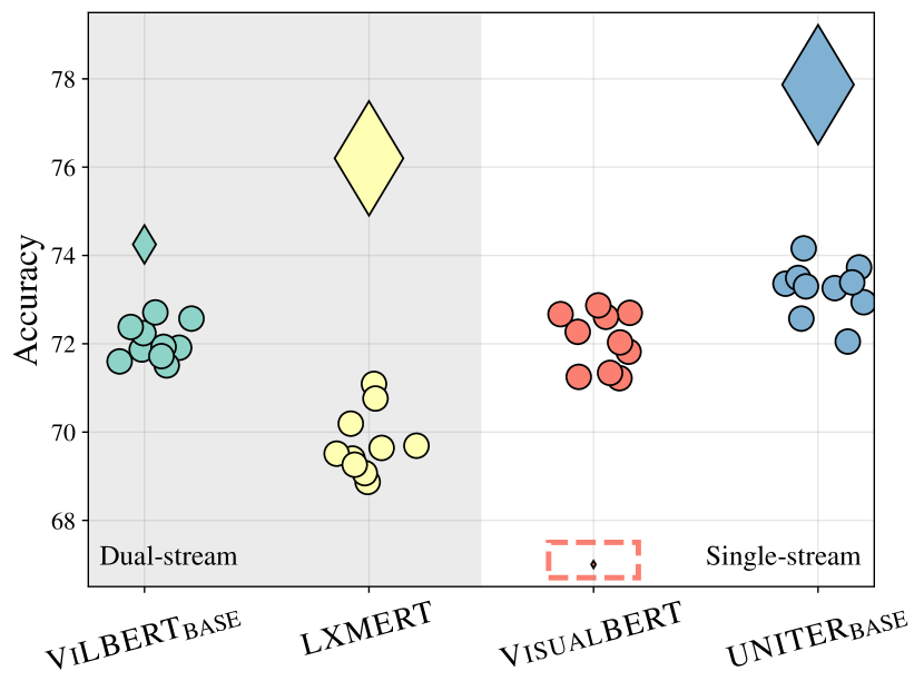
Figure 1: How does the amount of pretraining data affect downstream performance of V&L BERTs? We find that these models perform more similarly when trained in the same conditions. This plot shows the results from the papers ($\Diamond$), and when each model is pretrained 10 times on the Conceptual Captions dataset and fine-tuned once on the NLVR2 verification task ($\circ$). The area of a marker is proportional to the amount of pretraining data. The result from the VisualBERT paper is highlighted in a dashed box.

The first goal of this paper is to understand the mathematical differences between single- and dual-stream models. Our analysis leads to a unified framework in which currently proposed architectures, both single- and dual-stream, are particular instances. We then implement several of the proposed encoders within this framework to empirically measure their differences in a controlled environment. We believe this comparative analysis is crucial to better understand and guide future research of massive models in this vibrant area of AI, ensuring progress is not blurred by confounds.

In fact, there are many differences in the protocols used to train V&L BERTs. In order to better understand these models, we conduct a series of controlled studies to investigate whether differences in downstream performance is explained by: (i) the amount of pretraining data and the pretraining objectives (e.g., Figure 2); (ii) the hyperparameters used to control the learning process; (iii) the variance caused by random initialisation when pretraining (e.g., Figure 1), (iv) the variance due to fine-tuning multiple times on a downstream task; (v) being single- or dual-stream architectures; or (vi) the choice of the embedding layer.

In summary, our contributions in this paper are:

• We introduce a unified mathematical framework in which currently proposed V&L BERTs are only a subset of the possibilities.

• We release code for Volta (Visiolinguistic Transformer architectures), a PyTorch implementation of this framework in order to speed up research in multimodal pretraining.

• We conduct a series of controlled studies finding that several models perform similarly when trained under the same conditions.

• While we find that single- and dual-stream families perform equally well, performance can differ significantly between two models and the embedding layer plays a key role.

• However, these V&L BERTs are sensitive to weight initialisation and state-of-the-art claims should not be made from single runs.

2 Vision-and-Language BERTs

Given a sequence of tokens $\{w_{1},\dots,w_{T}\}$ and a set of visual features $\{\mathbf{v}_{1},\dots,\mathbf{v}_{K}\}$, a shared goal of V&L BERT models is to produce cross-modal representations that are useful for downstream tasks grounded in both modalities.

In this section, we first review how these models embed their inputs to the feature space. Next, we discuss the main differences in the encoders and, finally, highlight a variety of confounds that might affect the performance achieved by these models.

2.1 Input Embeddings

Language input

All V&L BERTs adopt the approach of BERT: The input sequence is first tokenized into sub-word units (Wu et al., 2016; Sennrich et al., 2016) and two special tokens $[\texttt{CLS}]$ and $[\texttt{SEP}]$ are added to generate the text sequence $\{[\texttt{CLS}],w_{1},\dots,w_{T},[\texttt{SEP}]\}$. The embedding of each token is then given by the sum of three learnable vectors, corresponding to its form, position in the sequence and segment (Devlin et al., 2019). In addition, VL-BERT Su et al. (2020) also adds the visual feature of the entire image to each token.

Vision input

Typically, visual inputs are also very similar across all V&L BERTs. For a given image, a pretrained object detector is used to extract regions of interest (RoIs), representing salient image regions. For each region, in addition to its feature vector, the object detector also returns the spatial location of its bounding box, which most V&L BERTs encode in different ways, analogously to the word position in the language modality. While most approaches present very similar ways to embed spatial locations, VL-BERT relies on a more complex geometry embedding and they are, instead, missing in VisualBERT Li et al. (2019). Some models also include a special feature $[\texttt{IMG}]$ that denotes the representation of the entire image (e.g., a mean-pooled visual feature with a spatial encoding corresponding to the full image). Finally, Pixel-BERT Huang et al. (2020) does not rely on an object detector but directly extracts a set of visual embeddings from the raw image.

2.2 Encoders

Single-stream encoders

The majority of V&L BERTs follow the single-stream paradigm (Su et al., 2020; Li et al., 2019; Chen et al., 2020; Li et al., 2020a; Zhou et al., 2020; Lin et al., 2020; Li et al., 2020b). Here, a standard BERT architecture is given the concatenation of the visual and linguistic features of an image–text pair as input (Figure 3a). This design allows for an early and unconstrained fusion of cross-modal information.

Dual-stream encoders

ViLBERT (Lu et al., 2019), LXMERT (Tan and Bansal, 2019), and ERNIE-ViL (Yu et al., 2021) are based on a dual-stream paradigm. Here, the visual and linguistic features are first processed by two independent stacks of Transformer layers. The resulting representations are then fed into cross-modal Transformer layers where intra-modal interactions are alternated with inter-modal interactions (see Figure 3b and c). Interestingly, both ViLBERT and LXMERT modelled inter-modal interactions in the same way: each stream first computes its query, key, and value matrices, before passing the keys and values to the other modality. By doing so, these models explicitly constrain interactions between modalities at each layer, inhibiting some of the interactions that are possible in a single-stream encoder while increasing their expressive power by separate sets of learnable parameters.

2.3 Pretraining Objectives

V&L BERTs are pretrained by jointly optimising multiple different self-supervised objectives over tokens and image regions through (weighted) scalarisation: $\mathscr{L}({\boldsymbol{\theta}})=\sum_{o}\lambda_{o}\mathscr{L}_{o}({\boldsymbol{\theta}})$. Here, ${\boldsymbol{\theta}}$ denotes a model’s parameters, $\mathscr{L}_{o}$ is the $o$-th objective, and $\lambda_{o}$ is its corresponding weight. Commonly adopted objectives are of three types: language, vision and cross-modal predictions.

For language prediction, BERT’s denoising masked language modelling (MLM) objective is typically used. MLM replaces some tokens with a [MASK] symbol, which are then predicted by using bidirectional text context and image regions.

The MLM objective has been extended to image regions via masked region modelling objectives. These typically take the form of either object classification or feature regression, with some papers showing benefits when modelling both (e.g., Chen et al. 2020). Some models, such as LXMERT, are also optimised over objects’ attributes prediction.

Finally, interactions between the two modalities are explicitly enforced by means of cross-modal objectives. The typical task here is that of image–text matching (ITM; e.g., Chen et al. 2020), which extends BERT’s next sentence prediction objective to V&L inputs: Given a sequence of tokens and a set of image regions, the model is tasked to predict whether the tokens describe the image.

2.4 Further Distinctions

So far, we have given an overview of the core components in V&L BERTs. However, there are several implementation differences between them.

For instance, LXMERT presents two main variations to the above description of dual-stream models. First, in its inter-modal layer, the parameters of the attention sub-layer are shared between the two streams. This results in the model learning a single function to contextualise image and text inputs, regardless of which modality plays the role of query or context. Second, its intra-modal layer only consists of the multi-head attention block.

Moreover, a wider range of choices can affect the performance of these models. From the object detector used (and whether it is also fine-tuned during pretraining), to the number of image regions and the maximum text sequence length, to the number of layers and their hidden sizes, to pooling methods and fine-tuning MLP sizes, to the use of text-only data, to optimisation hyperparameters (such as the number of pretraining epochs).

Another important distinction is the size and type of pretraining data, which can affect task performance (Figure 2). The size of pretraining datasets ranges from $3\text{M}$–$10\text{M}$ image–text pairs, over a range of pretraining tasks. The literature distinguishes between “in-domain” and “out-of-domain” data, each of which may consist of multiple datasets. An in-domain dataset overlaps with common downstream tasks, e.g. using VQAv2 (Goyal et al., 2017) as both a pretraining task and a downstream task, while out-of-domain datasets have no expected overlap, e.g. Conceptual Captions (Sharma et al., 2018).

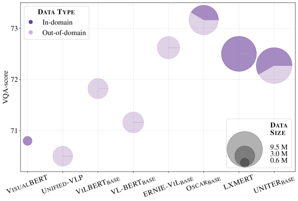
Figure 2: Comparison of proposed V&L BERTs on VQAv2 (most common downstream task) as a function of their pretraining data (size and type).

3 A Unified Framework

In this section, we unify the recently proposed single-stream and dual-stream architectures under the same mathematical framework. We start by reviewing the Transformer layer, which forms the core of these architectures, then we explain how this layer has been adapted to encode multimodal data in V&L BERTs, and introduce a gated bimodal Transformer layer that implements all of the architecture variants as special cases.

3.1 Transformer Layers

Transformer-based architectures consist of a stack of Transformer layers (Vaswani et al., 2017), each typically having a multi-head attention block ($\mathrm{MAB}$) and a feed-forward block ($\mathrm{FFB}$).

Multi-head attention block

Given $N_{q}$ query vectors, each of dimension $d_{q}$, $\mathbf{Q}\in\mathbb{R}^{N_{q}\times d_{q}}$, and $N_{v}$ key–value pairs $\mathbf{K}\in\mathbb{R}^{N_{v}\times d_{q}},\mathbf{V}\in\mathbb{R}^{N_{v}\times d_{v}}$, an attention function $\mathrm{Att}(\mathbf{Q},\mathbf{K},\mathbf{V})$ maps queries to output vectors with a scaled dot-product:

$$\mathrm{Att}(\mathbf{Q},\mathbf{K},\mathbf{V})=\omega\left(\mathbf{Q}\mathbf{K}^{\top}\right)\mathbf{V}$$ (1)

where $\omega$ denotes a row-wise, scaled softmax: $\omega_{i}(\cdot)=\mathrm{softmax}(\cdot/\sqrt{d_{q}})$. Here, $\mathbf{S}=\mathbf{Q}\mathbf{K}^{\top}\in\mathbb{R}^{N_{q}\times N_{v}}$ is a score matrix that measures the similarity between each pair of query and key vectors. The output of Eq. 1 is a weighted sum of $\mathbf{V}$, in which a value gets higher weight if its corresponding key has a larger dot product with the query.

Multi-head attention (MHA) extends this function by first projecting $\mathbf{Q},\mathbf{K},\mathbf{V}$ into $H$ different matrices and computing the attention of each projection (Eq. 1). These $H$ different output vectors are concatenated together ($[\mathbin{\|}]$) and the concatenation is projected with a linear transformation $\mathbf{W}^{O}$:

$$\begin{array}[]{c}\mathrm{MHA}(\mathbf{Q},\mathbf{K},\mathbf{V})=[\mathbf{O}_{1}\mathbin{\|}\dots\mathbin{\|}\mathbf{O}_{H}]\mathbf{W}^{O},\\ \text{where }\mathbf{O}_{h}=\mathrm{Att}\left(\mathbf{Q}\mathbf{W}^{Q}_{h},\mathbf{K}\mathbf{W}^{K}_{h},\mathbf{Q}\mathbf{W}^{V}_{h}\right).\end{array}$$ (2)

Here, $\{\mathbf{W}^{Q}_{h},\mathbf{W}^{K}_{h},\mathbf{W}^{V}_{h}\}^{H}_{h=1}$ and $\mathbf{W}^{O}$ are learned parameters. Usually, $\mathit{d_{q}=d_{v}=d}$, $\mathbf{W}^{O}\in\mathbb{R}^{d\times d}$, and $\mathbf{W}^{Q}_{h},\mathbf{W}^{K}_{h},\mathbf{W}^{V}_{h}\in\mathbb{R}^{d\times d_{a}}$ where $\mathit{d_{a}=d/H}$.

Finally, given inputs $\mathbf{X},\mathbf{Y}\in\mathbb{R}^{N\times d}$, a multi-head attention block is defined as:

$$\mathrm{MAB}(\mathbf{X},\mathbf{Y})=\mathrm{LN}(\mathbf{X}+\mathrm{MHA}(\mathbf{X},\mathbf{Y},\mathbf{Y})),$$ (3)

where $\mathrm{LN}$ is layer normalization (Ba et al., 2016).

Feed-forward block

For an input matrix $\mathbf{M}\in\mathbb{R}^{N\times d}$, the feed-forward block is given by:

$$\mathrm{FFB}(\mathbf{M})=\mathrm{LN}(\mathbf{M}+\mathrm{ReLU}(\mathbf{M}\mathbf{W}_{1})\mathbf{W}_{2}),$$ (4)

where $\mathbf{W}_{1},\mathbf{W}_{2}^{\top}\in\mathbb{R}^{d\times d_{\mathit{ff}}}$ are learnable matrices.

Standard Transformer layer

Let $\mathbf{X}\in\mathbb{R}^{N\times d}$ be an embedded input sequence, a standard Transformer layer performing self-attention is a parameterised function $f_{\theta}:\mathbb{R}^{N\times d}\rightarrow\mathbb{R}^{N\times d}$ such that:

$$f_{\theta}(\mathbf{X})=\mathrm{FFB}(\mathrm{MAB}(\mathbf{X},\mathbf{X})).$$ (5)

A stack of $L$ Transformer layers that encodes an input $\mathbf{X}$, such as BERT, is then seen as a sequence of $L$ Transformer layers, each parametrised by $\theta_{l}$:

$$\text{Encoder}(\mathbf{X})=f_{\theta_{L}}\circ\cdots\circ f_{\theta_{1}}(\mathbf{X}).$$ (6)

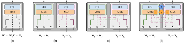
Figure 3: Visualisation of the (a) single-stream, (b) dual-stream intra-modal and (c) dual-stream inter-modal Transformer layers. (d) shows our gated bimodal layer. The inter-modal layer attends across modalities, while the intra-model layer attends within each modality. Ours can attend to either or both.

3.2 Single-stream Multimodal Transformers

Single-stream V&L BERTs extend BERT by concatenating the embedded visual inputs $\mathbf{X}_{\mathcal{V}}\in\mathbb{R}^{N_{\mathcal{V}}\times d}$ and the embedded textual inputs $\mathbf{X}_{\mathcal{L}}\in\mathbb{R}^{N_{\mathcal{L}}\times d}$ as a single input, hence the name “single-stream” (Figure 3a). Specifically, $\mathbf{X}=[\mathbf{X}_{\mathcal{L}}\mathbin{\|}\mathbf{X}_{\mathcal{V}}]\in\mathbb{R}^{N\times d}$, where $N=N_{\mathcal{L}}+N_{\mathcal{V}}$, and the attention is over both modalities (Figure 4a). Hence, all single-stream models are of the type defined in the previous section: $\text{Encoder}(\mathbf{X})$. The various approaches only differ in the initial V&L embeddings, the pretraining tasks, and the training data.

3.3 Dual-stream Multimodal Transformers

Both ViLBERT and LXMERT concurrently introduced inter-modal and intra-modal layers.

Inter-modal Transformer layer

The inter-modal layer explicitly models cross-modal interaction via a cross-modal attention module. Specifically, let $\mathcal{M}\in\{\mathcal{L},\mathcal{V}\}$ denote either the linguistic ($\mathcal{L}$) or the visual ($\mathcal{V}$) modality, and $\backslash\mathcal{M}$ its complementary one. The inter-modal multi-head attention for modality $\mathcal{M}$ is given by (Figure 3c):

$$\begin{array}[]{l}\mathbf{M}_{\mathcal{M}\backslash\mathcal{M}}=\mathrm{MAB}(\mathbf{X}_{\mathcal{M}},\mathbf{X}_{\backslash\mathcal{M}}).\end{array}$$ (7)

Note that the second input to the multi-head attention block (Eq. 3) is taken from the complementary modality, which means the keys $\mathbf{K}$ and values $\mathbf{V}$ in scaled dot-product attention (Eq. 1) operate across modalities (see Figure 4d and e). The remainder of this layer follows as from Eq. 4.

Intra-modal Transformer layer

The intra-modal layer, on the other hand, is a Transformer layer computing the attention of each modality independently (see Figure 3b). For a modality $\mathcal{M}$:

$$\begin{array}[]{l}\mathbf{M}_{\mathcal{M}\mathcal{M}}=\mathrm{MAB}(\mathbf{X}_{\mathcal{M}},\mathbf{X}_{\mathcal{M}}).\end{array}$$ (8)

The rest of the layer follows as in Eq. 4 for ViLBERT, while there is no $\mathrm{FFB}$ block in LXMERT.

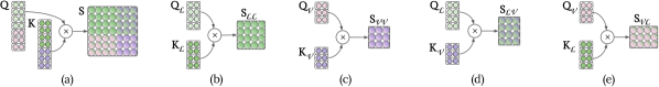
Figure 4: Visualisation of the score matrix for (a) single-stream, (b) text–text, (c) vision–vision, (d) text–vision, and (e) vision–text interactions. Shades of green denote the text modality, while purple ones denote the vision modality. Dual-stream scores are sub-matrices of the single-stream scores matrix.

3.4 Dual-stream Attentions as Restricted Single-stream Attention

Recall that in single-stream models the input to a Transformer layer is the concatenation of both modalities, $\mathbf{X}=[\mathbf{X}_{\mathcal{L}}\mathbin{\|}\mathbf{X}_{\mathcal{V}}]$. Therefore, in each single-stream attention head, the query representation is given by:

$$\mathbf{Q}=\mathbf{X}\mathbf{W}^{Q}=\begin{pmatrix}\mathbf{X}_{\mathcal{L}}\\ \mathbf{X}_{\mathcal{V}}\end{pmatrix}\mathbf{W}^{Q}=\begin{pmatrix}\mathbf{Q}_{\mathcal{L}}\\ \mathbf{Q}_{\mathcal{V}}\end{pmatrix}$$ (9)

where $\begin{pmatrix}\cdot_{\mathcal{L}}\\ \cdot_{\mathcal{V}}\end{pmatrix}$ are the language and visual sub-matrices of the input and the resulting output. A similar expression also holds for the keys $\mathbf{K}$ and values $\mathbf{V}$. We note that the score matrix $\mathbf{S}$ can be defined in terms of four sub-matrices (Figure 4a):

$$\mathbf{S}=\mathbf{Q}\mathbf{K}^{\top} =\begin{pmatrix}\mathbf{Q}_{\mathcal{L}}\\ \mathbf{Q}_{\mathcal{V}}\end{pmatrix}\begin{pmatrix}\mathbf{K}_{\mathcal{L}}^{\top}&\mathbf{K}_{\mathcal{V}}^{\top}\end{pmatrix}$$

$$=\begin{pmatrix}\mathbf{Q}_{\mathcal{L}}\mathbf{K}_{\mathcal{L}}^{\top}&\mathbf{Q}_{\mathcal{L}}\mathbf{K}_{\mathcal{V}}^{\top}\\ \mathbf{Q}_{\mathcal{V}}\mathbf{K}_{\mathcal{L}}^{\top}&\mathbf{Q}_{\mathcal{V}}\mathbf{K}_{\mathcal{V}}^{\top}\end{pmatrix}$$

$$=\begin{pmatrix}\mathbf{S}_{\mathcal{L}\mathcal{L}}&\mathbf{S}_{\mathcal{L}\mathcal{V}}\\ \mathbf{S}_{\mathcal{V}\mathcal{L}}&\mathbf{S}_{\mathcal{V}\mathcal{V}}\end{pmatrix}$$ (10)

Recall from Eq. 1 that the attention matrix is a normalised score matrix $\mathbf{S}$, so each single-stream layer computes both intra-modal (diagonal of $\mathbf{S}$) and inter-modal attention (anti-diagonal of $\mathbf{S}$). In other words, the dual-stream inter-modal and intra-modal attention functions act as restricted versions of the attention function in any single-stream layer (see Figure 4). As a result, by interleaving inter- and intra-modal layers, dual-stream models introduce an inductive bias towards which interactions the model enforces in each layer.

3.5 Gated Bimodal Transformer Layers

In the previous section, we showed that single-stream attention blocks capture both the inter-modal and intra-modal interactions, separately modelled by dual-stream architectures. We now introduce a general gated bimodal Transformer layer (Figure 3d), in which both single- and dual-stream layers are special cases. By doing so, we can define existing V&L BERTs within a single architecture, which allows us to implement and evaluate several of these models in a controlled environment (see next sections). In addition to textual $\mathbf{X}_{\mathcal{L}}$ and visual embeddings $\mathbf{X}_{\mathcal{V}}$, this layer takes a set of fixed binary variables $\{\boldsymbol{\gamma},\boldsymbol{\tau}\}$ as part of its input: $\boldsymbol{\gamma}=\{\gamma_{\mathcal{L}\mathcal{V}},\gamma_{\mathcal{V}\mathcal{L}},\gamma_{\mathcal{L}\mathcal{L}},\gamma_{\mathcal{V}\mathcal{V}}\}$, and $\boldsymbol{\tau}=\{\tau_{\mathit{MHA}},\tau_{\mathit{LN1}},\tau_{\mathit{FF}},\tau_{\mathit{LN2}}\}$. The $\boldsymbol{\gamma}$ values act as gates that regulate the cross-modal interactions within a layer, while the $\boldsymbol{\tau}$ values control whether the parameters are tied between modalities.

The main difference in our gated layer is in its attention functions, originally defined in Eq. 1 and Eq. 2. Here, we extend them to bimodal inputs with controllable multimodal interactions as:

where $\mathbf{W}^{O}_{\mathcal{L}}$ and $\mathbf{W}^{O}_{\mathcal{V}}$ are the language and vision output matrices. The attention output $\mathrm{Att}(\mathbf{Q},\mathbf{K},\mathbf{V})$, with a set of gating values $\gamma$ is:

$$\mathbf{O} =\mathrm{Att}\left(\begin{pmatrix}\mathbf{X}_{\mathcal{L}}\mathbf{W}^{Q}_{\mathcal{L}}\\ \mathbf{X}_{\mathcal{V}}\mathbf{W}^{Q}_{\mathcal{V}}\end{pmatrix},\begin{pmatrix}\mathbf{X}_{\mathcal{L}}\mathbf{W}^{K}_{\mathcal{L}}\\ \mathbf{X}_{\mathcal{V}}\mathbf{W}^{K}_{\mathcal{V}}\end{pmatrix},\begin{pmatrix}\mathbf{X}_{\mathcal{L}}\mathbf{W}^{V}_{\mathcal{L}}\\ \mathbf{X}_{\mathcal{V}}\mathbf{W}^{V}_{\mathcal{V}}\end{pmatrix};\boldsymbol{\gamma}\right)$$

$$=\mathrm{Att}\left(\begin{pmatrix}\mathbf{Q}_{\mathcal{L}}\\ \mathbf{Q}_{\mathcal{V}}\end{pmatrix},\begin{pmatrix}\mathbf{K}_{\mathcal{L}}\\ \mathbf{K}_{\mathcal{V}}\end{pmatrix},\begin{pmatrix}\mathbf{V}_{\mathcal{L}}\\ \mathbf{V}_{\mathcal{V}}\end{pmatrix};\boldsymbol{\gamma}\right)$$

$$=\omega\left(\mathbf{S}_{\boldsymbol{\gamma}}\right)\begin{pmatrix}\mathbf{V}_{\mathcal{L}}\\ \mathbf{V}_{\mathcal{V}}\end{pmatrix}$$ (12)

Recall from § 3.4 that the score matrix $\mathbf{S}_{\gamma}$ can be defined in terms of intra-modal and inter-modal submatrices. Here, the gating values $\boldsymbol{\gamma}=\{\gamma_{\mathcal{L}\mathcal{L}},\gamma_{\mathcal{L}\mathcal{V}},\gamma_{\mathcal{V}\mathcal{L}},\gamma_{\mathcal{V}\mathcal{V}}\}$ define the permitted intra-modal and inter-modal interactions. Let $\varepsilon\rightarrow-\infty$, $\mathbf{S}_{\boldsymbol{\gamma}}$ is given by:

$$\mathbf{S}_{\boldsymbol{\gamma}} =\begin{pmatrix}\varepsilon^{\gamma_{\mathcal{L}\mathcal{L}}}\mathbf{S}_{\mathcal{L}\mathcal{L}}&\varepsilon^{\gamma_{\mathcal{L}\mathcal{V}}}\mathbf{S}_{\mathcal{L}\mathcal{V}}\\ \varepsilon^{\gamma_{\mathcal{V}\mathcal{L}}}\mathbf{S}_{\mathcal{V}\mathcal{L}}&\varepsilon^{\gamma_{\mathcal{V}\mathcal{V}}}\mathbf{S}_{\mathcal{V}\mathcal{V}}\end{pmatrix}$$ (13)

That is, when an attention gate $\gamma$ is set to $1$, the corresponding sub-matrix tends to $-\infty$, while it is unaltered when $\gamma$ is set to $0$. By having a sub-matrix that tends to $-\infty$, we can effectively compute the row-wise softmax – i.e., the attention – over the other sub-matrix, hence recovering the inter- and intra-modal attentions. This is similar to the input masking applied in autoregressive Transformer decoders (Vaswani et al., 2017).

This formulation allows us to control the degree of inter- and intra-modal attention within a layer, allowing us to define existing architectures within a unified mathematical framework. We can recover an inter-modal block (Eq. 7) by setting $\gamma_{\mathcal{L}\mathcal{V}}=\gamma_{\mathcal{V}\mathcal{L}}=0$ and $\gamma_{\mathcal{L}\mathcal{L}}=\gamma_{\mathcal{V}\mathcal{V}}=1$. Similarly, the single-stream block (Eq. 3) can be recovered by setting $\boldsymbol{\gamma}=\mathbf{0}$ and tying the learnable parameters ($\boldsymbol{\tau}=\mathbf{1}$) between the two streams (e.g., $\mathbf{W}^{Q}_{\mathcal{L}}=\mathbf{W}^{Q}_{\mathcal{V}}=\mathbf{W}^{Q}$ in each attention head).

Furthermore, the gated bimodal Transformer layer allows us to model a superset of the few combinations considered thus far for cross-modal fusion by multimodal transformer encoders. One may explore asymmetric streams in which the two modalities interact differently with the bimodal inputs, or explore different ways of interleaving conventional single- and dual-stream blocks, or even different levels of parameter sharing. For example, asymmetric vision-and-language layers might be beneficial for navigation (e.g., Hill et al. 2021) or language-conditioned image generation (e.g., Cho et al. 2020). An exploration of these possibilities is left for future work.

4 Experimental Setup

In this section, we present the experimental setup for our controlled studies on V&L encoders.

Volta

In order to facilitate research and development of V&L pretraining, we release Volta (Visiolinguistic Transformer architectures), an implementation of our unified framework in PyTorch (Paszke et al., 2019). Our code is built on top of the ViLBERT-MT repository, based on PyTorch-Transformers, due to its support to a wide range of V&L tasks. We stress that it is important, for this study, to have a unified implementation that allows us to remove possible confounds due to implementation details and effectively measure differences given by the proposed architectures.

Implementation details

V&L BERTs typically extract image features using a Faster R-CNN (Ren et al., 2015) trained on the Visual Genome dataset (VG; Krishna et al. 2017), either with a ResNet-$101$ (He et al., 2016) or a ResNeXT-$152$ backbone (Xie et al., 2017). The number of features varies from $10$ to $100$. Our models are trained with $36$ regions of interest extracted by a Faster R-CNN with a ResNet-$101$ backbone (Anderson et al., 2018). Each model is initialized with the parameters of BERT, following the approaches described in the original papers. Randomly initialized weights are initialized following the standard approach in PyTorch-Transformers (on which these models built on): fully-connected and embedding layers are initialized from a normal distribution with mean $0.0$ and standard deviation $0.02$, bias vectors are initially set to $0.0$, and the Layer Normalization weight vector to $1.0$. We train all models on $4$ NVIDIA P$100$ GPUs and rely on gradient accumulation to obtain larger batches when needed. The parameter sets giving the best validation performance based on the pretraining objective are used for downstream tasks.

Dataset	Image Source	Train	Test	Metric
VQAv2	COCO	655K	448K	VQA-score
GQA	COCO+Flickr	1.1M	12.6K	Accuracy
RefCOCO+	COCO	120K	10.6K	Accuracy
RefCOCOg	COCO	80K	9.6K	Accuracy
NLVR2	Web Crawled	86K	7K	Accuracy
SNLI-VE	Flickr	529K	17.9K	Accuracy
COCO	COCO	567K	1K	Recall@1
Flirckr30k	Flickr	145K	1K	Recall@1

Table 1: Statistics of the downstream V&L tasks.

Pretraining

As discussed in § 2.4, V&L BERTs have been pretrained on datasets of varying size and type. In this paper, we pretrain all of our models on the Conceptual Captions dataset (CC; Sharma et al. 2018), which consists of $3.3\text{M}$ images with weakly-associated captions automatically collected from billions of web pages. This stands in contrast to other datasets, e.g. COCO (Lin et al., 2014) or VQA (Antol et al., 2015), where the images are strongly-associated with crowdsourced captions or question–answer pairs. The Conceptual Captions dataset is a good candidate for learning generic multimodal representations because of its size, that it was scraped from the Web, and that it has a broad coverage of subject matter. Note that due to broken links, and a subsequent pruning phase, where images also found in the test sets of common V&L tasks are removed, we pretrain all our models on $2.77\text{M}$ image–caption pairs from Conceptual Captions.

Downstream evaluation tasks

We consider the most common tasks used to evaluate V&L BERTs, spanning four groups: vocab-based VQA (Goyal et al., 2017; Hudson and Manning, 2019), image–text retrieval (Lin et al., 2014; Plummer et al., 2015), referring expression (Kazemzadeh et al., 2014; Mao et al., 2016) and multimodal verification  (Suhr et al., 2019; Xie et al., 2019). See Table 1 for details. For each model, the parameter set giving the best performance in the validation set was used for test.

5 Results

We perform carefully controlled experiments to investigate the possible reasons for the reported difference in performance between V&L BERTs.

5.1 Unified Data and Reimplementation

We start by examining the performance of V&L BERTs pretrained on the same $2.7$M CC dataset. Recall from Figure 2 that V&L BERTs have been pretrained on different combinations of datasets, which may explain most of the claimed differences in downstream task performance. Here, we evaluate three models with official released code: ViLBERT, LXMERT and VL-BERT.

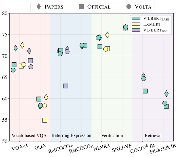
Figure 5: Unified data and reimplementation results. Performance of selected V&L BERTs on multiple tasks from the original papers ($\Diamond$), and when pretrained on $2.7\text{M}$ Conceptual Captions with their official code ($\square$) or in Volta ($\circ$).

Same data, similar performance

Figure 5 shows the results of controlling the pretraining data and pretraining tasks. The results from the papers are reported ($\Diamond$), alongside our training of these models using the official code ($\square$). There is a drop in performance for the models we trained on the VQAv2, NLVR2, and image retrieval tasks, compared to the performance reported in the papers. This is not surprising given that the $\square$ models were pretrained on less data than the papers. In particular, given that ViLBERT was also pretrained on CC but with more image–text pairs, our results corroborate previous studies showing diminishing returns with pretraining data size (e.g., Lu et al. 2019; Li et al. 2020a). However, the claimed performance gaps between these models narrows when they are pretrained on the same data. For instance, according to the literature, LXMERT was clearly the best model in VQA tasks, which is likely due to its use of large, in-domain data and a VQA pretraining objective.

Volta implementation

We also implemented these models in Volta and trained them using their official procedures and hyperparameters. Figure 5 shows that the performance of each of these models ($\circ$) closely follows the official implementations in these downstream tasks, confirming the correctness of our framework. There are, however, some larger differences for some of the tasks: in VQAv2, we now see that ViLBERT performs slightly worse than the other models in (contrarily to what we obtained with the official code), and in GQA, LXMERT closes the gap with ViLBERT. ViLBERT’s performance on NLVR2 and COCO image retrieval increases by $2$–$3$ points in the Volta framework. As Volta is based on the ViLBERT code base, these differences might be due to weight initialisation, an hypothesis that we test in later sections.

With this first study, we have seen that the performance of these V&L BERTs is similar when they are trained on the same data. Moreover, we demonstrated the correctness of our implementations in Volta, in which these models are built following the unified framework introduced in § 3. Nevertheless, there are still many possible confounds in the training procedures adopted by these models that might interfere with a fair comparison of these architectures. In the next section, we control these variables to unmask the true gains introduced by a number of multimodal encoders.

5.2 Controlled Setup

We define a fixed set of hyperparameters to evaluate ViLBERT, LXMERT, VL-BERT, VisualBERT, and UNITER on four downstream tasks: VQAv2, RefCOCO+, NLVR2 and Flickr30K.

• Inputs: Each model used a different maximum number of tokens and LXMERT did not have an overall [IMG] feature. We fix the same maximum number of tokens and add the [IMG] feature to each architecture.

• Encoders: We noticed that ViLBERT used higher dimensional representations for the visual stream. We fix the same dimension as in the linguistic stream for a comparison that is fairer comparison against LXMERT, and more intuitive with the single-stream models.

• Pooling: While VL-BERT is the only architecture that does not have a pooling layer, other V&L BERTs use it for the image–text matching objective. We fix the models to use use multiplicative pooling (Lu et al., 2019) for all the models in order to separately learn sentence-level and image-level representations and also model their interactions.

• Pretraining objectives: Each model uses a different set of pretraining objectives. We fix them to three: MLM, masked object classification with KL-divergence, and ITM.

• Fine-tuning: We fine-tune each model using the same protocols and sizes for the MLPs.

• Hyperparameters: While ViLBERT and VL-BERT were originally pretrained for $10$ epochs, LXMERT was pretrained for $20$. We fix the number of pretraining epochs to $10$, and set other hyperparameters, e.g., learning rate or its warm-up proportion, to a set of values from the original papers that led to smooth training of all the models, with training curves that closely followed the ones obtained with the original hyperparameters.

Model		VQAv2		RefCOCO+		NLVR2		Flickr30k
		test-dev		testd		test-P		test IR	test TR
ViLBERT${}_{\textsc{BASE}}$		68.7		71.4		72.4		59.8	76.7
LXMERT		67.1		68.8		69.1		50.4	62.5
VL-BERT${}_{\textsc{BASE}}$		68.3		71.1		72.6		57.9	68.5
VisualBERT		68.2		69.7		71.3		61.1	75.5
UNITER${}_{\textsc{BASE}}$		68.8		71.9		72.9		60.9	74.2

Table 2: Results with our controlled setup. Each model is pretrained using the Volta framework with the same fixed hyperparameters on the $2.7$M CC dataset, and fine-tuned on downstream tasks.

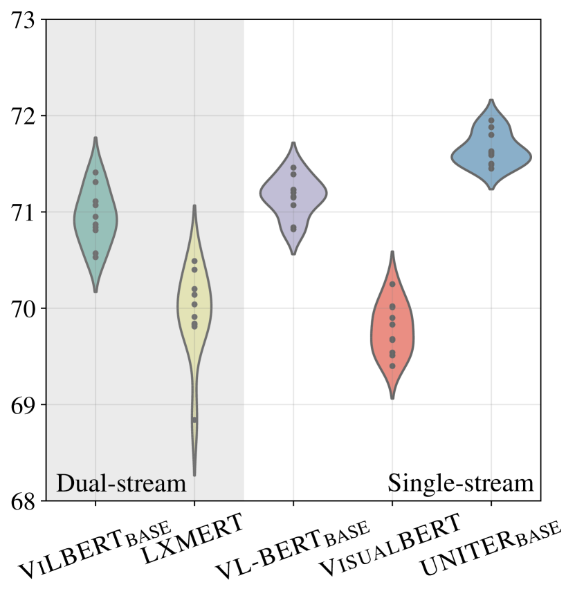
(a) RefCOCO+

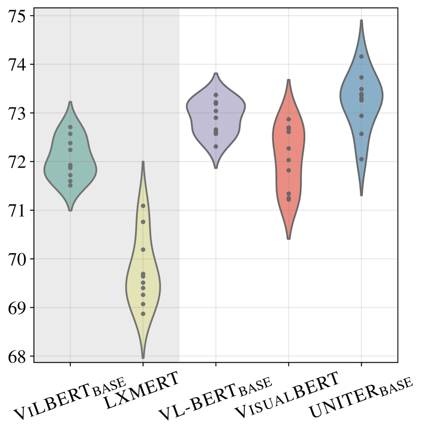
(b) NLVR2

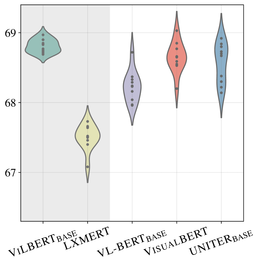
(c) VQAv2

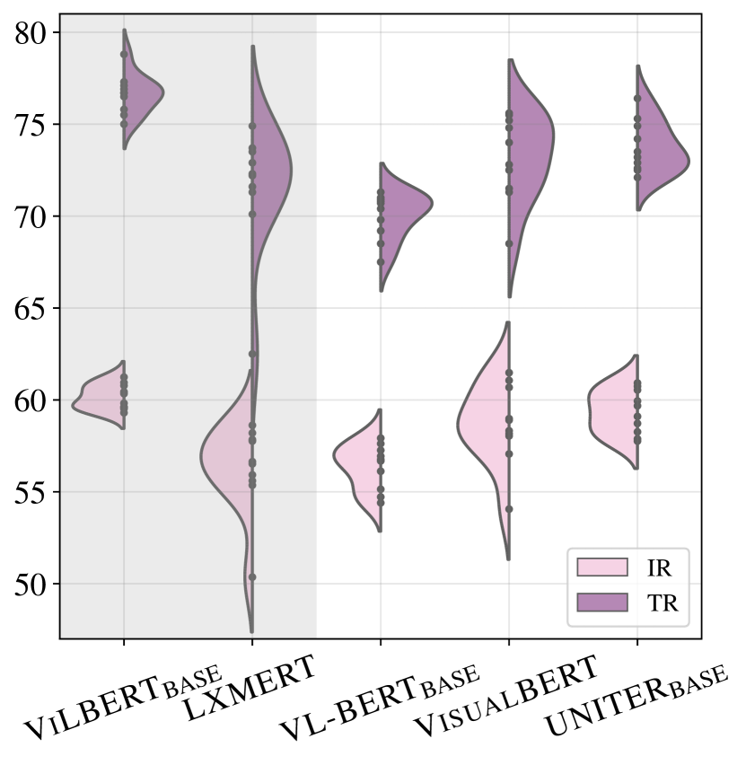
(d) Flickr30k

Figure 6: Pretraining variance of V&L BERTs. Each model is pretrained $10$ times and fine-tuned once.

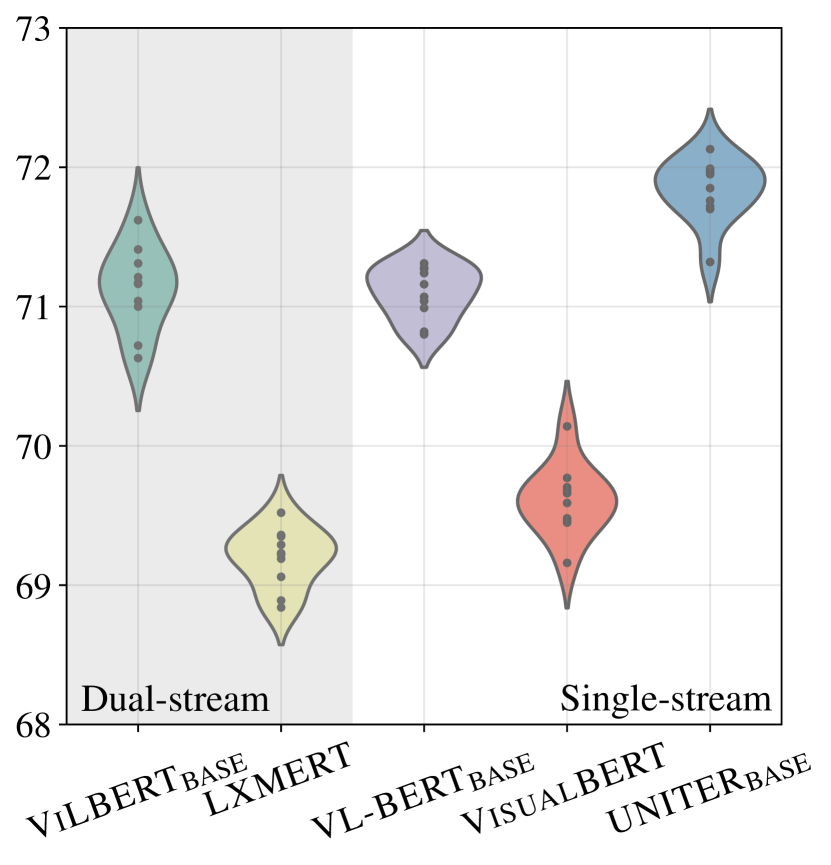
(a) RefCOCO+

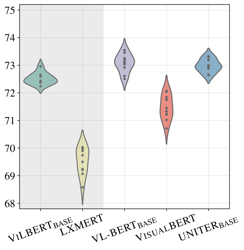
(b) NLVR2

Figure 7: Fine-tuning variance of V&L BERTs on RefCOCO+ and NLVR2. Each model is pretrained once and fine-tuned $10$ times on each task.

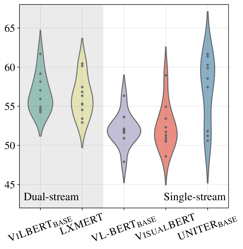
(a) Pretraining

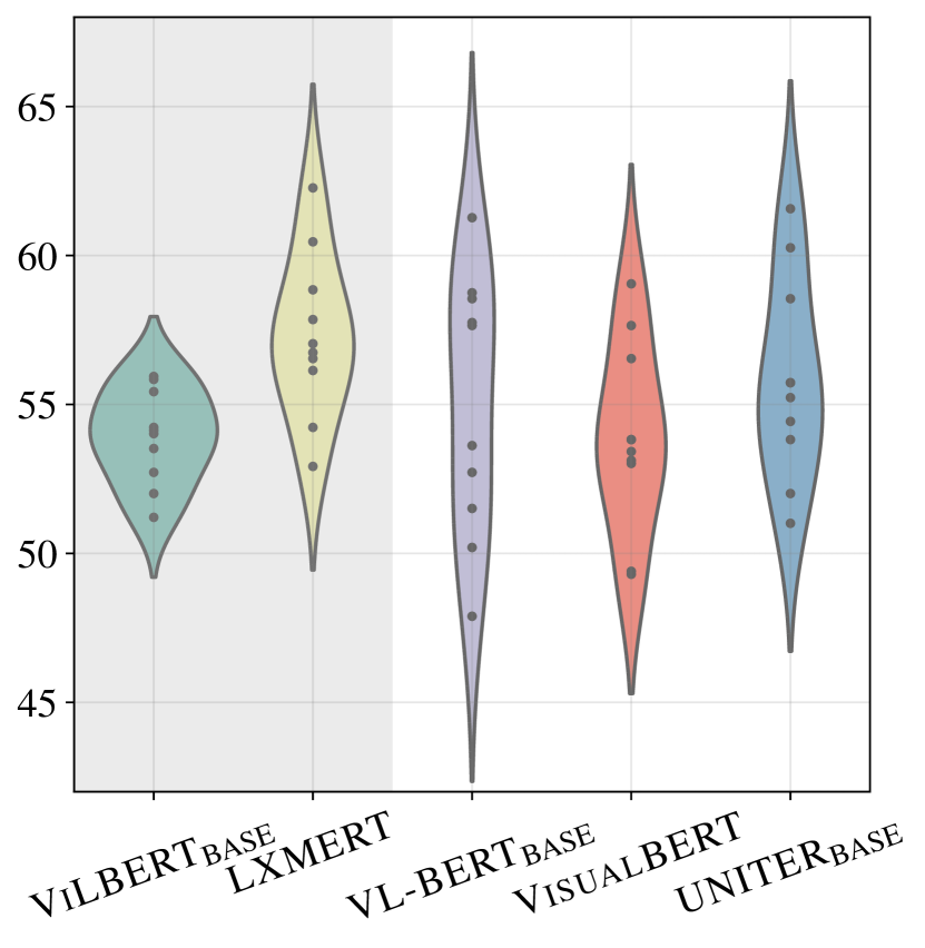
(b) Fine-tuning

Figure 8: Variance of V&L BERTs on the Constrastive Set of NLVR2, when each model is pretrained $10$ times and fine-tuned once (a), or pretrained once and fine-tuned $10$ times (b).

Results

Table 2 shows the results of our controlled study. First, we note that the performance of ViLBERT and VL-BERT is similar compared to training with their original hyperparameters. In fact, VQAv2 performance improves for ViLBERT, showing that dual-stream models do not require different sizes in the two streams. VL-BERT also performs similarly to its official setup, showing that the additional ITM pretraining objective in our controlled setup does not hurt downstream task performance (contrarily to the results reported in their paper). We do, however, note that LXMERT performs worse on NLVR2 and VQAv2 in our controlled setup than with its original hyperparameters, suggesting that LXMERT may require more pretraining steps to converge. Overall, the results show that most of the examined models perform similarly in our controlled setup, compared to the official setups.

5.3 Fine-tuning Variance

We now turn our attention to the effect of fine-tuning variance on task performance. It has been observed that the fine-tuning of BERT is sensitive to randomness in initialisation and data ordering (Dodge et al., 2020). Here, we investigate the sensitivity of the five models used in the controlled study. We fine-tune each model $10$ times on the RefCOCO+ and NLVR2 tasks by varying the seed. This changes training data order and the weight initialisation of the classification layer. Figure 7 shows violin plots of the distribution of results, in which the dots represent the experimental observations. We also report an average standard deviation of $0.3$ points for these models across both tasks. However, the minimum and the maximum scores of a given model often differ by $1$ or more points, showing how a single fine-tuning run of these models can lead to incorrect conclusions.

5.4 Pretraining Variance

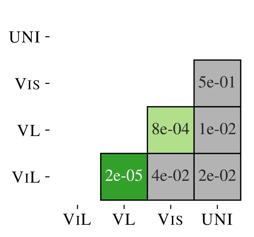
(a) VQAv2

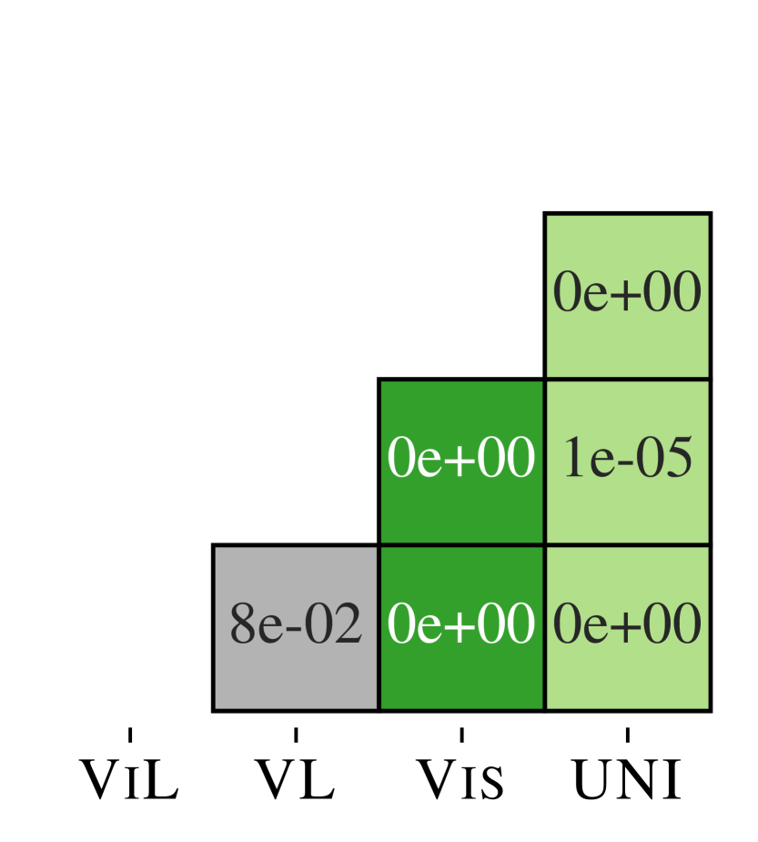
(b) RefCOCO+

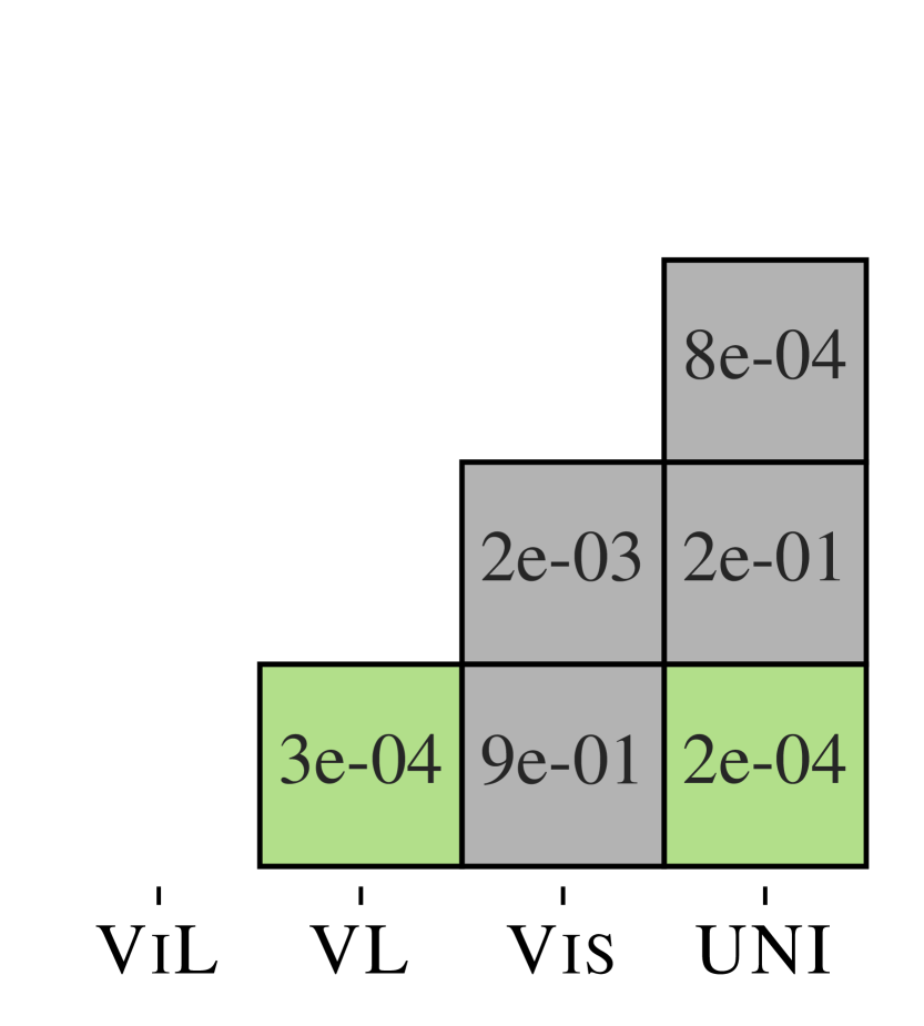
(c) NLVR2

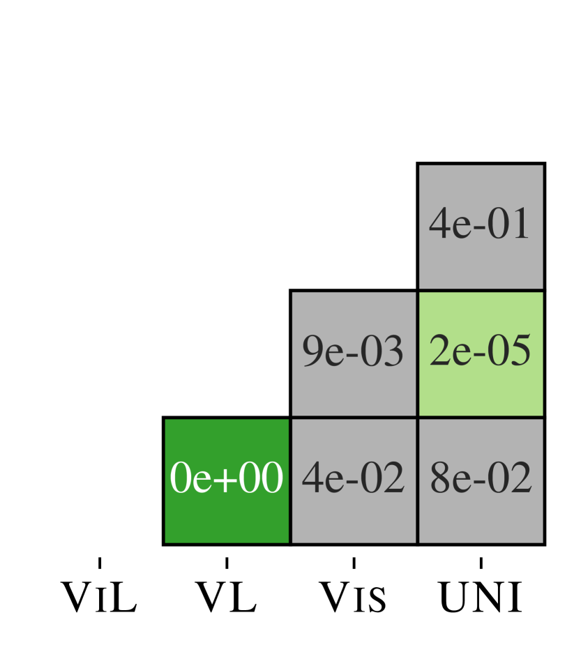
(d) Flickr30k IR

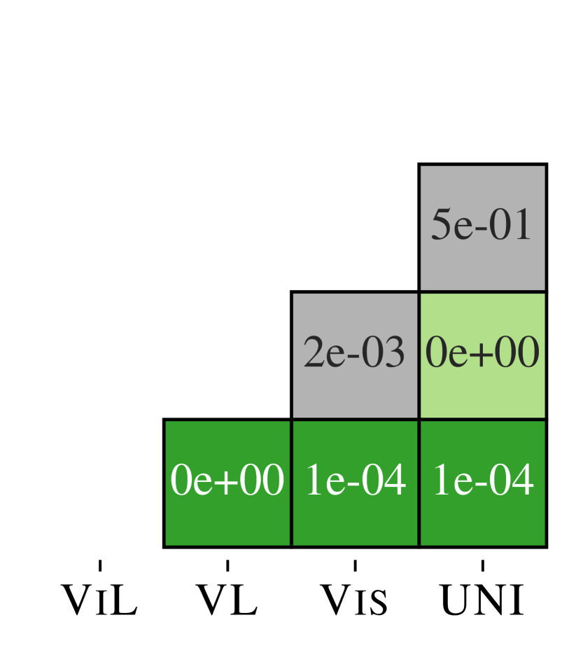
(e) Flickr30k TR

Figure 9: Exact test between any two V&L BERTs. Each box shows the p-value for the corresponding pair of models. Green boxes denote statistical significance at $0.005$ after Bonferroni correction. Boxes are dark green if the model in the y-axis outperforms the one in the x-axis, and vice versa for light green.

In the previous section, we found substantial variance in the performance of V&L BERTs across $10$ fine-tuning runs. We now investigate if the pretraining phase is similarly affected by different runs. Here, each model in our controlled setup is pretrained $10$ times and fine-tuned once on four tasks: VQAv2, RefCOCO+, NLVR2, and Flickr30K image–text retrieval. By varying the seed, we modify training data order as well as all the layers that are not initialised from BERT (e.g., the visual embeddings, the masked object classification head and the ITM head in single-stream models). Figure 6 shows violin plots for each task. We start by noting that our first pretraining run (Table 2) of LXMERT was the worst one (its text retrieval recall on Flickr30K is $10$ points lower than its mean). We also confirm that LXMERT has slower convergence rate, with its task performance after $10$ epochs showing the largest variance among the V&L BERTs we tested. On the other hand, we find that some of these architectures are less prone to variance caused by pretraining seed, such as ViLBERT for VQA and retrieval tasks, and UNITER for referring expression. Nevertheless, the performance of all of these models can vary by more than $1$ point in several tasks solely due to random initialisation.

5.5 Evaluating Local Decision Boundaries

Previous work has shown that state-of-the-art systems can exploit systematic gaps in the data to learn simple decision rules that let them achieve high performance on test data Gururangan et al. (2018); Geva et al. (2019); Ribeiro et al. (2019). In an effort to more accurately estimate model performance, Gardner et al. (2020) proposed contrast sets: datasets in which existing test instances have small but label-changing modifications in order to characterise the correct decision boundary near them. Figure 8 shows the performance of our analysed models on the NLVR2 contrast set. Similar to Gardner et al. (2020), we see that LXMERT loses around $15$ points when evaluated on perturbed samples. Furthermore, models that performed much better on the standard test set now achieve comparable performance to LXMERT, showing that they exploited systematic gaps. That is, all of these V&L BERTs would perform similarly when evaluated on out-of-distribution data.

5.6 Single- or Dual-stream Architectures

Dataset	Single/Dual Stream		V&L BERTs
	F-test	p-value	F-test	p-value
VQAv2	11.40	1.7e-03	12.75	8.0e-06∗
RefCOCO+	0.10	7.6e-01	111.61	2.7e-18∗
NLVR2	8.28	6.5e-03	13.41	5.0e-06∗
Flickr30k IR	9.64	3.6e-03	13.27	5.0e-06∗
Flickr30k TR	31.14	2.0e-06∗	29.74	7.5e-10∗

Table 3: ANOVA between single- and dual-stream architectures (left) and between all the tested V&L BERTs (right). ^∗ denotes significant results at $p<0.005$ after Bonferroni correction.

One of the key design choices that distinguishes V&L BERTs is the number of “streams” used by the encoder to process visual and linguistic inputs. Lu et al. (2019) showed how their single-stream baseline performed worse than their dual-stream ViLBERT architecture, while Chen et al. (2020) claimed single-stream UNITER outperformed ViLBERT. Our controlled study across several tasks and different pretraining initialisations allows us to provide an answer grounded with statistical tests. To do so, we split the models in dual- and single-stream architectures and run a one-way ANOVA (Table 3). After Bonferroni correction, we only find statistical difference at $p<0.005$ Benjamin et al. (2018) between these two groups for the Flickr30K text retrieval task.

On the other hand, running the same test among the various V&L BERTs, without grouping them as single- or dual-stream architectures, returns statistical significance in each task (Table 3). This table tells us that the null hypothesis, the models have the same average performance, does not hold. However, it does not allow us to discern where statistical differences lie. To do so, we conduct a post-hoc exact test at significance level $p<0.005$. Figure 9 shows the corresponding pair-wise p-values and highlights significant differences between any two models after Bonferroni correction. For instance, ViLBERT is significantly different compared to all other models in text retrieval on Flickr30k, while UNITER is significantly different on RefCOCO+.

5.7 The Importance of the Embeddings

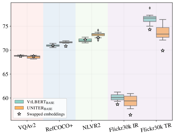
Figure 10: Results of swapping ViLBERT and UNITER embeddings ($\star$) compared to their performance when pretrained $10$ times (box plots).

Finally, our controlled setup leads us to an interesting finding: the embedding layer (§ 2.1) plays a crucial role in the final performance of V&L BERTs. In fact, the only difference among VL-BERT, VisualBERT and UNITER in our setup is their embedding layer. Figure 6 and Figure 7 show that this can have a drastic impact on the downstream performance although the literature has given little attention to this detail. For instance, Chen et al. (2020) claim that the main contribution of UNITER is the set of pretraining tasks, while our results, wherein all the models are trained on the same pretraining tasks, highlight that their embedding layer is an important confound on final performance. Interestingly, VisualBERT is the only model that does not encode the locations of regions of interest in its embeddings. This leads it to considerably lower performance on RefCOCO+, showing that this information is extremely useful for this task.

Given this result, we conduct one additional experiment to see whether the embedding layer biased our conclusion for dual- and single-stream performance. To test this, we swap the embedding layers of ViLBERT (best dual-stream) and UNITER (overall better single-stream) with each other, which we pretrain and fine-tune once (Figure 10). Similar to our previous results, embeddings are especially important for the tasks of referring expression and retrieval. However, no single embedding layer performs better, corroborating that dual- and single-stream architectures perform on par and showing that different embedding strategies are necessary to maximise performance in these two families of V&L BERTs.

5.8 Limitations

All the experiments in this paper are limited to models that use a specific type of pretrained and frozen visual encoder. While most V&L BERTs follow this paradigm, some studies find beneficial to jointly learn the visual encoder with language Su et al. (2020); Huang et al. (2020); Radford et al. (2021); Kim et al. (2021). In addition, we only consider base architecture variants (initialised with BERT${}_{\textit{BASE}}$) and pretrained on CC. Studying the effects of visual encoders, pretraining data and larger models is left as future work.

Although we expect longer pretraining would be beneficial for every model, in our controlled setup, we pretrain each model for $10$ epochs to reduce resource consumption. Here, we also constrain our hyperparameter search over a small grid of values that have been used in the literature. Finally, we leave a thorough, controlled study of the various pretraining objectives to future work.

6 Reproducibility and the Environment

From the perspective of reproducible research, there are several advantages to using the Volta framework for V&L encoders. First, Volta reduces confounds due to differences in implementations, while also enabling fair comparisons with related work. Second, visual and textual data only need to be preprocessed once instead of creating model-specific formats for every V&L BERT.

From a financial perspective, the costs involved in pretraining hampers contributions from many academic institutions and deters the evaluation of multiple trained models, which we showed to be extremely important for V&L BERTs. We estimate that pretraining a single model $10\times$ in our controlled setup for $4$ downstream tasks requires a $4$-GPU machine on AWS for two months, at a cost of $\sim\$6{,}000$, corresponding to $200$ GPU-compute days. Fortunately, we had access to an internal server, but the our experiments still required $1{,}500$ GPU days for training and evaluation. While we were able to reduce the financial costs, there are severe environmental and carbon footprint costs in V&L pretraining (Strubell et al., 2019).

We hope that Volta will serve as a basis for research in V&L pretraining, enabling easy and fair comparisons across architectures, and ensuring that progress is not obfuscated by confounds.

7 Conclusion

We introduced and implemented a unified mathematical framework, under which recently proposed V&L BERTs can be specified as special cases. We conducted a series of controlled studies within this framework to better understand the differences between several models. We found that the performance of the considered models varies significantly due to random initialisation, in both pretraining and fine-tuning. We also found that these models achieve similar performance when trained with the same hyperparameters and data. Notably, some models outperform others but we found that (a) single- and dual-stream model families are on par, and (b) embedding layers play a crucial role towards a model’s final performance.

Our fast-paced field rewards the contribution of new methods and state-of-the-art results Rogers and Augenstein (2020), which often contrasts with controlled comparisons and training multiple models for variance estimation. In this paper, we showed that several methods for vision-and-language representation learning do not significantly differ when compared in a controlled setting. This finding echoes similar studies of variants of LSTMs Greff et al. (2017) and Transformers Narang et al. (2021) that are not significantly better than the original models. Looking to the future, we recommend that new V&L BERTs are pretrained on similar datasets, and that researchers report fine-tuning variance, in addition to their best performing model. We hope that our findings will encourage more controlled evaluations of newly proposed architectures for vision-and-language and beyond.

References

- Anderson et al. (2018) Peter Anderson, Xiaodong He, Chris Buehler, Damien Teney, Mark Johnson, Stephen Gould, and Lei Zhang. 2018. Bottom-up and top-down attention for image captioning and visual question answering. In Proceedings of the IEEE/CVF Conference on Computer Vision and Pattern Recognition (CVPR), pages 6077–6086.
- Antol et al. (2015) Stanislaw Antol, Aishwarya Agrawal, Jiasen Lu, Margaret Mitchell, Dhruv Batra, C. Lawrence Zitnick, and Devi Parikh. 2015. VQA: Visual Question Answering. In Proceedings of the IEEE/CVF International Conference on Computer Vision (ICCV), pages 2425–2433.
- Ba et al. (2016) Jimmy Lei Ba, Jamie Ryan Kiros, and Geoffrey E Hinton. 2016. Layer normalization. arXiv preprint arXiv:1607.06450.
- Benjamin et al. (2018) Daniel J Benjamin, James O Berger, Magnus Johannesson, Brian A Nosek, E-J Wagenmakers, Richard Berk, Kenneth A Bollen, Björn Brembs, Lawrence Brown, Colin Camerer, et al. 2018. Redefine statistical significance. Nature human behaviour, 2(1):6–10.
- Chen et al. (2020) Yen-Chun Chen, Linjie Li, Licheng Yu, Ahmed El Kholy, Faisal Ahmed, Zhe Gan, Yu Cheng, and Jingjing Liu. 2020. Uniter: Universal image-text representation learning. In European Conference on Computer Vision, pages 104–120. Springer.
- Cho et al. (2020) Jaemin Cho, Jiasen Lu, Dustin Schwenk, Hannaneh Hajishirzi, and Aniruddha Kembhavi. 2020. X-LXMERT: Paint, Caption and Answer Questions with Multi-Modal Transformers. In Proceedings of the 2020 Conference on Empirical Methods in Natural Language Processing (EMNLP), pages 8785–8805, Online. Association for Computational Linguistics.
- Devlin et al. (2019) Jacob Devlin, Ming-Wei Chang, Kenton Lee, and Kristina Toutanova. 2019. BERT: Pre-training of deep bidirectional transformers for language understanding. In Proceedings of the 2019 Conference of the North American Chapter of the Association for Computational Linguistics: Human Language Technologies, Volume 1 (Long and Short Papers), pages 4171–4186, Minneapolis, Minnesota. Association for Computational Linguistics.
- Dodge et al. (2020) Jesse Dodge, Gabriel Ilharco, Roy Schwartz, Ali Farhadi, Hannaneh Hajishirzi, and Noah Smith. 2020. Fine-tuning pretrained language models: Weight initializations, data orders, and early stopping. arXiv preprint arXiv:2002.06305.
- Gardner et al. (2020) Matt Gardner, Yoav Artzi, Victoria Basmov, Jonathan Berant, Ben Bogin, Sihao Chen, Pradeep Dasigi, Dheeru Dua, Yanai Elazar, Ananth Gottumukkala, Nitish Gupta, Hannaneh Hajishirzi, Gabriel Ilharco, Daniel Khashabi, Kevin Lin, Jiangming Liu, Nelson F. Liu, Phoebe Mulcaire, Qiang Ning, Sameer Singh, Noah A. Smith, Sanjay Subramanian, Reut Tsarfaty, Eric Wallace, Ally Zhang, and Ben Zhou. 2020. Evaluating models’ local decision boundaries via contrast sets. In Findings of the Association for Computational Linguistics: EMNLP 2020, pages 1307–1323, Online. Association for Computational Linguistics.
- Geva et al. (2019) Mor Geva, Yoav Goldberg, and Jonathan Berant. 2019. Are we modeling the task or the annotator? an investigation of annotator bias in natural language understanding datasets. In Proceedings of the 2019 Conference on Empirical Methods in Natural Language Processing and the 9th International Joint Conference on Natural Language Processing (EMNLP-IJCNLP), pages 1161–1166, Hong Kong, China. Association for Computational Linguistics.
- Goyal et al. (2017) Yash Goyal, Tejas Khot, Douglas Summers-Stay, Dhruv Batra, and Devi Parikh. 2017. Making the V in VQA matter: Elevating the role of image understanding in Visual Question Answering. In Proceedings of the IEEE/CVF Conference on Computer Vision and Pattern Recognition (CVPR), pages 6325–6334.
- Greff et al. (2017) Klaus Greff, Rupesh K. Srivastava, Jan Koutník, Bas R. Steunebrink, and Jürgen Schmidhuber. 2017. Lstm: A search space odyssey. IEEE Transactions on Neural Networks and Learning Systems, 28(10):2222–2232.
- Gururangan et al. (2018) Suchin Gururangan, Swabha Swayamdipta, Omer Levy, Roy Schwartz, Samuel Bowman, and Noah A. Smith. 2018. Annotation artifacts in natural language inference data. In Proceedings of the 2018 Conference of the North American Chapter of the Association for Computational Linguistics: Human Language Technologies, Volume 2 (Short Papers), pages 107–112, New Orleans, Louisiana. Association for Computational Linguistics.
- He et al. (2016) Kaiming He, Xiangyu Zhang, Shaoqing Ren, and Jian Sun. 2016. Deep residual learning for image recognition. In Proceedings of the IEEE/CVF Conference on Computer Vision and Pattern Recognition (CVPR), pages 770–778.
- Hill et al. (2021) Felix Hill, Olivier Tieleman, Tamara von Glehn, Nathaniel Wong, Hamza Merzic, and Stephen Clark. 2021. Grounded language learning fast and slow. In International Conference on Learning Representations.
- Huang et al. (2020) Zhicheng Huang, Zhaoyang Zeng, Bei Liu, Dongmei Fu, and Jianlong Fu. 2020. Pixel-bert: Aligning image pixels with text by deep multi-modal transformers. arXiv preprint arXiv:2004.00849.
- Hudson and Manning (2019) Drew A. Hudson and Christopher D. Manning. 2019. Gqa: A new dataset for real-world visual reasoning and compositional question answering. In Proceedings of the IEEE/CVF Conference on Computer Vision and Pattern Recognition (CVPR), pages 6700–6709.
- Kazemzadeh et al. (2014) Sahar Kazemzadeh, Vicente Ordonez, Mark Matten, and Tamara Berg. 2014. ReferItGame: Referring to objects in photographs of natural scenes. In Proceedings of the 2014 Conference on Empirical Methods in Natural Language Processing (EMNLP), pages 787–798, Doha, Qatar. Association for Computational Linguistics.
- Kim et al. (2021) Wonjae Kim, Bokyung Son, and Ildoo Kim. 2021. Vilt: Vision-and-language transformer without convolution or region supervision. arXiv preprint arXiv:2102.03334.
- Krishna et al. (2017) Ranjay Krishna, Yuke Zhu, Oliver Groth, Justin Johnson, Kenji Hata, Joshua Kravitz, Stephanie Chen, Yannis Kalantidis, Li-Jia Li, David A Shamma, et al. 2017. Visual genome: Connecting language and vision using crowdsourced dense image annotations. International Journal of Computer Vision, 123(1):32–73.
- Li et al. (2020a) Gen Li, Nan Duan, Yuejian Fang, Ming Gong, and Daxin Jiang. 2020a. Unicoder-vl: A universal encoder for vision and language by cross-modal pre-training. Proceedings of the AAAI Conference on Artificial Intelligence, 34(07):11336–11344.
- Li et al. (2019) Liunian Harold Li, Mark Yatskar, Da Yin, Cho-Jui Hsieh, and Kai-Wei Chang. 2019. Visualbert: A simple and performant baseline for vision and language. arXiv preprint arXiv:1908.03557.
- Li et al. (2020b) Xiujun Li, Xi Yin, Chunyuan Li, Pengchuan Zhang, Xiaowei Hu, Lei Zhang, Lijuan Wang, Houdong Hu, Li Dong, Furu Wei, et al. 2020b. Oscar: Object-semantics aligned pre-training for vision-language tasks. In European Conference on Computer Vision, pages 121–137. Springer.
- Lin et al. (2020) Junyang Lin, An Yang, Yichang Zhang, Jie Liu, Jingren Zhou, and Hongxia Yang. 2020. Interbert: Vision-and-language interaction for multi-modal pretraining. arXiv preprint arXiv:2003.13198.
- Lin et al. (2014) Tsung-Yi Lin, Michael Maire, Serge Belongie, James Hays, Pietro Perona, Deva Ramanan, Piotr Dollár, and C. Lawrence Zitnick. 2014. Microsoft coco: Common objects in context. In European Conference on Computer Vision, pages 740–755, Cham. Springer.
- Lu et al. (2019) Jiasen Lu, Dhruv Batra, Devi Parikh, and Stefan Lee. 2019. Vilbert: Pretraining task-agnostic visiolinguistic representations for vision-and-language tasks. In Advances in Neural Information Processing Systems, pages 13–23. Curran Associates, Inc.
- Lu et al. (2020) Jiasen Lu, Vedanuj Goswami, Marcus Rohrbach, Devi Parikh, and Stefan Lee. 2020. 12-in-1: Multi-task vision and language representation learning. In Proceedings of the IEEE/CVF Conference on Computer Vision and Pattern Recognition (CVPR), pages 10434–10443.
- Mao et al. (2016) J. Mao, J. Huang, A. Toshev, O. Camburu, A. Yuille, and K. Murphy. 2016. Generation and comprehension of unambiguous object descriptions. In Proceedings of the IEEE/CVF Conference on Computer Vision and Pattern Recognition (CVPR), pages 11–20.
- Narang et al. (2021) Sharan Narang, Hyung Won Chung, Yi Tay, William Fedus, Thibault Fevry, Michael Matena, Karishma Malkan, Noah Fiedel, Noam Shazeer, Zhenzhong Lan, Yanqi Zhou, Wei Li, Nan Ding, Jake Marcus, Adam Roberts, and Colin Raffel. 2021. Do transformer modifications transfer across implementations and applications? arXiv preprint arXiv:2102.11972.
- Paszke et al. (2019) Adam Paszke, Sam Gross, Francisco Massa, Adam Lerer, James Bradbury, Gregory Chanan, Trevor Killeen, Zeming Lin, Natalia Gimelshein, Luca Antiga, Alban Desmaison, Andreas Kopf, Edward Yang, Zachary DeVito, Martin Raison, Alykhan Tejani, Sasank Chilamkurthy, Benoit Steiner, Lu Fang, Junjie Bai, and Soumith Chintala. 2019. Pytorch: An imperative style, high-performance deep learning library. In H. Wallach, H. Larochelle, A. Beygelzimer, F. d'Alché-Buc, E. Fox, and R. Garnett, editors, Advances in Neural Information Processing Systems, pages 8024–8035. Curran Associates, Inc.
- Plummer et al. (2015) Bryan A. Plummer, Liwei Wang, Chris M. Cervantes, Juan C. Caicedo, Julia Hockenmaier, and Svetlana Lazebnik. 2015. Flickr30k entities: Collecting region-to-phrase correspondences for richer image-to-sentence models. In Proceedings of the IEEE/CVF International Conference on Computer Vision (ICCV), page 2641–2649, USA. IEEE Computer Society.
- Qi et al. (2020) Di Qi, Lin Su, Jia Song, Edward Cui, Taroon Bharti, and Arun Sacheti. 2020. Imagebert: Cross-modal pre-training with large-scale weak-supervised image-text data. arXiv preprint arXiv:2001.07966.
- Radford et al. (2021) Alec Radford, Jong Wook Kim, Chris Hallacy, Aditya Ramesh, Gabriel Goh, Sandhini Agarwal, Girish Sastry, Amanda Askell, Pamela Mishkin, Jack Clark, Gretchen Krueger, and Ilya Sutskever. 2021. Learning transferable visual models from natural language supervision. arXiv preprint arXiv:2103.00020.
- Ren et al. (2015) Shaoqing Ren, Kaiming He, Ross Girshick, and Jian Sun. 2015. Faster r-cnn: Towards real-time object detection with region proposal networks. In C. Cortes, N. D. Lawrence, D. D. Lee, M. Sugiyama, and R. Garnett, editors, Advances in Neural Information Processing Systems, pages 91–99. Curran Associates, Inc.
- Ribeiro et al. (2019) Marco Tulio Ribeiro, Carlos Guestrin, and Sameer Singh. 2019. Are red roses red? evaluating consistency of question-answering models. In Proceedings of the 57th Annual Meeting of the Association for Computational Linguistics, pages 6174–6184, Florence, Italy. Association for Computational Linguistics.
- Rogers and Augenstein (2020) Anna Rogers and Isabelle Augenstein. 2020. What can we do to improve peer review in NLP? In Findings of the Association for Computational Linguistics: EMNLP 2020, pages 1256–1262, Online. Association for Computational Linguistics.
- Sennrich et al. (2016) Rico Sennrich, Barry Haddow, and Alexandra Birch. 2016. Neural machine translation of rare words with subword units. In Proceedings of the 54th Annual Meeting of the Association for Computational Linguistics (Volume 1: Long Papers), pages 1715–1725, Berlin, Germany. Association for Computational Linguistics.
- Sharif Razavian et al. (2014) Ali Sharif Razavian, Hossein Azizpour, Josephine Sullivan, and Stefan Carlsson. 2014. Cnn features off-the-shelf: An astounding baseline for recognition. In Proceedings of the IEEE/CVF Conference on Computer Vision and Pattern Recognition (CVPR) Workshops, pages 512–519.
- Sharma et al. (2018) Piyush Sharma, Nan Ding, Sebastian Goodman, and Radu Soricut. 2018. Conceptual captions: A cleaned, hypernymed, image alt-text dataset for automatic image captioning. In Proceedings of the 56th Annual Meeting of the Association for Computational Linguistics (Volume 1: Long Papers), pages 2556–2565, Melbourne, Australia. Association for Computational Linguistics.
- Strubell et al. (2019) Emma Strubell, Ananya Ganesh, and Andrew McCallum. 2019. Energy and policy considerations for deep learning in NLP. In Proceedings of the 57th Annual Meeting of the Association for Computational Linguistics, pages 3645–3650, Florence, Italy. Association for Computational Linguistics.
- Su et al. (2020) Weijie Su, Xizhou Zhu, Yue Cao, Bin Li, Lewei Lu, Furu Wei, and Jifeng Dai. 2020. Vl-bert: Pre-training of generic visual-linguistic representations. In International Conference on Learning Representations.
- Suhr et al. (2019) Alane Suhr, Stephanie Zhou, Ally Zhang, Iris Zhang, Huajun Bai, and Yoav Artzi. 2019. A corpus for reasoning about natural language grounded in photographs. In Proceedings of the 57th Annual Meeting of the Association for Computational Linguistics, pages 6418–6428, Florence, Italy. Association for Computational Linguistics.
- Tan and Bansal (2019) Hao Tan and Mohit Bansal. 2019. LXMERT: Learning cross-modality encoder representations from transformers. In Proceedings of the 2019 Conference on Empirical Methods in Natural Language Processing and the 9th International Joint Conference on Natural Language Processing (EMNLP-IJCNLP), pages 5100–5111, Hong Kong, China. Association for Computational Linguistics.
- Vaswani et al. (2017) Ashish Vaswani, Noam Shazeer, Niki Parmar, Jakob Uszkoreit, Llion Jones, Aidan N Gomez, Łukasz Kaiser, and Illia Polosukhin. 2017. Attention is all you need. In I. Guyon, U. V. Luxburg, S. Bengio, H. Wallach, R. Fergus, S. Vishwanathan, and R. Garnett, editors, Advances in Neural Information Processing Systems, pages 5998–6008. Curran Associates, Inc.
- de Vries et al. (2017) Harm de Vries, Florian Strub, Sarath Chandar, Olivier Pietquin, Hugo Larochelle, and Aaron Courville. 2017. Guesswhat?! visual object discovery through multi-modal dialogue. In Proceedings of the IEEE Conference on Computer Vision and Pattern Recognition (CVPR), pages 4466–4475.
- Wu et al. (2016) Yonghui Wu, Mike Schuster, Zhifeng Chen, Quoc V Le, Mohammad Norouzi, Wolfgang Macherey, Maxim Krikun, Yuan Cao, Qin Gao, Klaus Macherey, et al. 2016. Google’s neural machine translation system: Bridging the gap between human and machine translation. arXiv preprint arXiv:1609.08144.
- Xie et al. (2019) Ning Xie, Farley Lai, Derek Doran, and Asim Kadav. 2019. Visual entailment: A novel task for fine-grained image understanding. arXiv preprint arXiv:1901.06706.
- Xie et al. (2017) Saining Xie, Ross Girshick, Piotr Dollár, Zhuowen Tu, and Kaiming He. 2017. Aggregated residual transformations for deep neural networks. In Proceedings of the IEEE/CVF Conference on Computer Vision and Pattern Recognition (CVPR), pages 5987–5995.
- Yu et al. (2021) Fei Yu, Jiji Tang, Weichong Yin, Yu Sun, Hao Tian, Hua Wu, and Haifeng Wang. 2021. Ernie-vil: Knowledge enhanced vision-language representations through scene graph. Proceedings of the AAAI Conference on Artificial Intelligence.
- Yu et al. (2018) Licheng Yu, Zhe Lin, Xiaohui Shen, Jimei Yang, Xin Lu, Mohit Bansal, and Tamara L. Berg. 2018. Mattnet: Modular attention network for referring expression comprehension. In Proceedings of the IEEE Conference on Computer Vision and Pattern Recognition (CVPR), pages 1307–1315.
- Zellers et al. (2019) Rowan Zellers, Yonatan Bisk, Ali Farhadi, and Yejin Choi. 2019. From recognition to cognition: Visual commonsense reasoning. In Proceedings of the IEEE/CVF Conference on Computer Vision and Pattern Recognition (CVPR), pages 6713–6724.
- Zhou et al. (2020) Luowei Zhou, Hamid Palangi, Lei Zhang, Houdong Hu, Jason Corso, and Jianfeng Gao. 2020. Unified vision-language pre-training for image captioning and vqa. Proceedings of the AAAI Conference on Artificial Intelligence, 34(07):13041–13049.
- Zhu et al. (2016) Y. Zhu, O. Groth, M. Bernstein, and L. Fei-Fei. 2016. Visual7w: Grounded question answering in images. In 2016 IEEE Conference on Computer Vision and Pattern Recognition (CVPR), pages 4995–5004.