The Impact of Time Series Length and Discretization on Longitudinal Causal Estimation Methods

Abstract

The use of observational time series data to assess the impact of multi-time point interventions is becoming increasingly common as more health and activity data are collected and digitized via wearables, social media, and electronic health records. Such time series may involve hundreds or thousands of irregularly sampled observations. One common analysis approach is to simplify such time series by first discretizing them into sequences before applying a discrete-time estimation method that adjusts for time-dependent confounding. In certain settings, this discretization results in sequences with many time points; however, the empirical properties of longitudinal causal estimators have not been systematically compared on long sequences. We compare three representative longitudinal causal estimation methods on simulated and real clinical data. Our simulations and analyses assume a Markov structure and that longitudinal treatments/exposures are binary-valued and have at most a single jump point. We identify sources of bias that arise from temporally discretizing the data and provide practical guidance for discretizing data and choosing between methods when working with long sequences. Additionally, we compare these estimators on real electronic health record data, evaluating the impact of early treatment for patients with a life-threatening complication of infection called sepsis.

1 Introduction

Sequence length can have major practical implications for the performance of discrete-time longitudinal statistical methods. For example, a well-known drawback of inverse probability weighting (IPW) methods [9, 24], and of importance sampling methods more broadly, is that estimator variance can grow exponentially with sequence length [4]. However, the performance of other popular longitudinal causal estimators has not been systematically compared on sequences comprising tens or hundreds of time points, such as those occurring in observational health settings, e.g., [15, 13, 11, 29]. Further, the primary means for controlling sequence length, increasing the width of the discrete time bins, is known to introduce bias in certain settings [28]. Thus, practitioners must balance bias and variance concerns when making discretization decisions. We investigate this bias/variance trade-off.

We evaluate the impact of discretization and sequence length on three popular longitudinal causal estimators: the aforementioned IPW estimators, iterative regression estimators based directly on the g-computation formula (IR) (sometimes referred to as the parametric g-computation formula [21]), and targeted minimum loss-based estimators (TMLE) [35, 34]. Our goal is to provide practical guidance for choosing between estimators and making discretization decisions. We address the question: How does discretization bin width — and, by extension, sequence length — affect bias and variance for each of these estimators? To answer this question, we first use simulations to compare the performance of these estimators as we vary the discretization bin width (Section 5). Next, under a Markov assumption, we analytically identify one source of potential bias incurred by the IR and TMLE methods as a result of discretization and provide recommendations for avoiding this bias (Section 6). Finally, we compare these estimators on a real clinical causal estimation problem using electronic health record (EHR) data with up to 73 discrete time points (Section 7).

This work builds on a growing literature examining the behavior of longitudinal causal estimation methods. Gottesman et al. [5] and Tran et al. [33] both presented comparisons of longitudinal estimation methods on simulated and observational health data and both considered the effect of sequence length on estimator performance; however, both studies focused on how increasing the time horizon, and thus changing the estimand, increases the likelihood of finite sample positivity violations as fewer participants follow the treatment regime of interest. While we comment briefly on finite sample positivity violations, our focus is on the effect of discretization decisions for a fixed estimand and without changing the number of participants who follow the treatment regime of interest. Further, Tran et al. [33] used fixed length sequences with up to 6 time points and Gottesman et al. [5] used variable length sequences with an average of 13 time points. In this work, we consider simulated sequences with up to 257 time points and real clinical data with up to 73 time points. Sofrygin et al. [29] examined the effect of discretization decisions on a particular TMLE estimator in an observational health setting. Their analysis included sequences with up to 143 time points, but did not compare performance across estimators. The combination of these related works and our paper may provide guidance for the design and analysis of studies involving non-experimental longitudinal data.

Another area in which causal inference methods have been applied to long sequential data is in off-policy evaluation of reinforcement learning (RL) algorithms. Off-policy evaluation refers to estimating the expected reward (i.e., outcome) under a particular policy of interest from observational data that was generated according to a different policy. This is equivalent to longitudinal causal inference from observational data. While off-policy evaluation is frequently done using IPW-based estimators, recent work has used doubly-robust estimators in order to reduce variance. For example, Jiang and Li [10] and Thomas and Brunskill [32] presented such doubly-robust estimators, observing that they reduced variance relative to IPW estimators. The estimators used in Jiang and Li [10] and Thomas and Brunskill [32] differ from those considered in this paper in that they assume certain nuisance parameters were estimated while the evaluation policy was being learned. [22] consider the related problem of extrapolating an optimal treatment policy from one population to a biologically similar population where observations are made less frequently.

A final important area of related work is in the development of estimators that operate on irregularly sampled continuous time data. For example, Soleimani et al. [30] and Schulam and Saria [27] modeled both the treatment and feature values, as well as the timing of observations using Bayesian non-parametric methods. An advantage of these methods is that they obviate the need to discretize longitudinal data; however, they require modeling the joint distribution of all time-varying covariates which generally requires stronger modeling assumptions than here. While the focus of our work is on the proper application of sequential methods, we view the development of continuous-time methods as an important complementary direction which becomes especially important in settings with insufficient domain knowledge to make discretization decisions.

2 Motivating application: measuring the effect of early antibiotics for patients with sepsis

This work is motivated by recent studies that use electronic health records to estimate the cumulative impact of an exposure or treatment over time, while adjusting for confounders, e.g., [15, 30, 27, 11, 13, 5, 29]. In particular, we are motivated by the study of how early treatment affects patients hospitalized with a life-threatening complication of infection called sepsis. Sepsis is characterized by organ failure caused by infection and is one of the leading causes of in-hospital mortality in the United States [20]. Several observational studies have suggested that early initiation of antibiotic therapy improves outcomes for patients with sepsis [3, 14, 16]; however, these studies have treated the decision of when to initiate antibiotics as a single time-point intervention and do not account for time-varying confounding. In contrast, we treat the decision to initiate antibiotics as a time-varying treatment and estimate the effect of delayed versus early antibiotics while adjusting for potential time-varying confounding and right censoring.

We used EHR data from 9,523 patients admitted to the emergency department (ED) with sepsis to estimate the population average treatment effect (ATE) of receiving antibiotics within one hour of admission versus not receiving antibiotics during the first 13 hours after admission. (In the latter regime, antibiotics may be given after the first 13 hours.) As sepsis is primarily characterized by organ dysfunction, our outcome was an aggregate measure of cumulative organ dysfunction measured 73 hours after admission. As in our simulated data, we compare the performance of the estimators listed above under different discretizations of the EHR data.

3 Problem definition

3.1 Time discretization and notation

We consider how changing the temporal discretization of our data affects discrete-time estimators. We do this by first defining a “finest discretization” of time and then considering various coarser discretizations created by taking a subset of time points from the finest discretization. The finest discretization consists of a sequence of $T^{*}$ equally-spaced measurements with $\delta^{*}$ time between successive measurements. We index these measurements by $t=1,2,\dots,T^{*}$. For example, if time is measured in hours, then the first measurement time ($t=1$) is $0$ hours after baseline, the second ($t=2$) is $\delta^{*}$ hours after baseline,…, and the last ($t=T^{*}$) is $(T^{*}-1)\delta^{*}$ hours after baseline. This finest discretization (also called the “uncoarsened discretization”) is the gold standard under which our estimand of interest is defined.

Using the finest discretization, consider a sequence of binary-valued treatment variables $\bar{A}(\delta^{*})=[A(\delta^{*})_{1},...,A(\delta^{*})_{T^{*}}]$. We are interested in the expected value of an outcome variable $Y$ under a hypothetical treatment regime where everyone in the target population is set to follow a particular static treatment sequence $\bar{a}(\delta^{*})=[a(\delta^{*})_{1},\dots,a(\delta^{*})_{T^{*}}]$ [21, 7]. Using potential outcomes notation, this can be written as $\mathbb{E}[Y^{\bar{a}(\delta^{*})}]$, where $Y^{\bar{a}(\delta^{*})}$ is the (counterfactual) value of $Y$ had the treatment sequence been set to $\bar{a}(\delta^{*})$.

We would like to estimate $\mathbb{E}[Y^{\bar{a}(\delta^{*})}]$ using observational data that has been temporally discretized with $\delta\geq\delta^{*}$ time between successive time points, where $\delta$ is a multiple of $\delta^{*}$. Because $\delta$ is a multiple of $\delta^{*}$, the sequence with bin width $\delta$ contains a subset of time points from the finest discretization. The resulting coarsened sequence has length $T(\delta)=\lfloor\frac{\delta^{*}}{\delta}(T^{*}-1)\rfloor+1$. We denote the dataset discretized at bin width $\delta$ by $\mathcal{D}(\delta)=\{(V_{i},\bar{A}(\delta)_{i},\bar{L}(\delta)_{i},Y_{i})\}_{i=1}^{N}$, where for each $i$, $V_{i}$ represents baseline features, $\bar{A}(\delta)_{i}=[A(\delta)_{i,1},...,A(\delta)_{i,T(\delta)}]$ represents a sequence of treatment values, $\bar{L}(\delta)_{i}=[L(\delta)_{i,1},...,L(\delta)_{i,T(\delta)}]$ represents a sequence of time-varying features, and $Y_{i}$ represents the outcome of interest. We sometimes suppress the dependence of sequence length $T(\delta)$, treatment sequence $\bar{A}(\delta)$, feature sequence $\bar{L}(\delta)$, and dataset $\mathcal{D}(\delta)$ on $\delta$. The temporal ordering of variables is assumed to be: $V_{i},L_{i,1},A_{i,1},...,L_{i,T},A_{i,T},Y_{i}$. We assume that the vectors $(V_{i},\bar{A}_{i},\bar{L}_{i},Y_{i}),i=1,\dots,N$ are independent, identically distributed draws from an unknown joint distribution $P$. Where it does not cause ambiguity, we drop the index $i$.

Denote by $\bar{L}_{t}=[L_{1},...,L_{t}]$ the feature sequence up to and including time point $t$, $\underline{L}_{t}=[L_{t},...,L_{T}]$ the feature sequence from time point $t$ onward, and $\bar{L}_{j:k}=[L_{j},...,L_{k}]$ the feature sequence from time point $j$ through time point $k$, with analogous definitions for $\bar{A}_{t}$, $\underline{A}_{t}$, and $\bar{A}_{j:k}$. Additionally, we will occasionally refer to the potential outcome of $L_{t}$ under treatment sequence $\bar{a}$ denoted by $L_{t}^{\bar{a}}$, as well as the potential outcome of $L_{t}$ when only the treatment subsequence $\bar{a}_{j:k}$ is set, denoted by $L_{t}^{\bar{a}_{j:k}}$.

We address the following question: how does the discretization bin width $\delta$ — and, by extension, sequence length $T(\delta)$ — affect various estimators of $\psi=\mathbb{E}[Y^{\bar{a}(\delta^{*})}]$? We address this question by starting with the finest discretization (small $\delta$ and large $T(\delta)$) and gradually moving to a coarse one (large $\delta$ and small $T(\delta)$). In general, changing $T(\delta)$, either by changing the outcome variable as in Gottesman et al. [5] and Tran et al. [33], or by changing $\delta$ as in Sofrygin et al. [29], may change both the estimand and the number of participants that follow $\bar{a}$. As our goal is to isolate the impact that $\delta$ has on an estimator for a fixed estimand and without changing the number of participants who follow $\bar{a}$, we focus on estimands that are not impacted by changing $\delta$. We assume that both the observed treatment sequence $\bar{A}$ (with probability 1) and the treatment regime $\bar{a}$ are binary sequences that start at 0, may jump to 1 at some point, and remain at 1 thereafter; we assume that this holds under the finest discretization, which implies that it holds under any coarser discretization. This type of restricted treatment sequence can be used to represent the initiation of a treatment at a given time — i.e., the jump time.

Throughout, we consider static treatment regimes $\bar{a}(\delta^{*})$ that represent the rules “treat immediately”, “never treat”, and “do not treat before time $k\delta^{*}$”. The rule “treat immediately” is represented by the sequence of treatments $[1,\dots,1]$, the rule “never treat” is represented by the sequence of treatments $[0,\dots,0]$, and the rule “do not treat before time $k\delta^{*}$” is represented by the sequence of treatments consisting of $0$’s through time $k\delta^{*}$ and subsequent treatments unspecified. For each of these regimes, it follows that the estimand $\mathbb{E}[Y^{\bar{a}(\delta^{*})}]$ (which is defined using the finest discretization) equals the corresponding quantity $\mathbb{E}[Y^{\bar{a}(\delta)}]$ (defined in terms of the coarser discretization $\delta>\delta*$) as long as the coarser discretization includes the measurement time $0$, $(T^{*}-1)\delta^{*}$, or $k\delta^{*}$, respectively.

3.2 Identifiability assumptions

All quantities in this paragraph are with respect to the finest discretization, i.e., $\delta^{*}$, which we suppress in the notation for clarity. In order for our estimand $\mathbb{E}[Y^{\bar{a}}]$ to be identifiable from the observed data under the finest discretization, we make three assumptions about the data generating distributions. Discussion of these assumptions and their definitions can be found in Hernan and Robins [7]. First, we make the consistency assumption that $Y^{\bar{a}}=Y$ if $\bar{A}=\bar{a}$, and $\bar{L}_{t}^{\bar{a}}=\bar{L}_{t}$ if $\bar{A}_{t-1}=\bar{a}_{t-1}$. Second, we assume that there is a positive probability of $A_{t}$ jumping to $1$ or remaining $0$ given the history up to time $t$ (positivity) or formally, $0<P(A_{t}=1\mid A_{t-1}=0,\bar{L}_{t},V)<1$ almost surely, for all $t$, where $A_{0}$ and $L_{0}$ are defined as 0 by convention. Finally, we assume sequential exchangeability which can be written as $(Y^{\bar{a}},\underline{L}_{t+1}^{\bar{a}})\perp\!\!\!\perp A_{t}\mid\bar{A}_{t-1}=\bar{a}_{t-1},\bar{L}_{t},V$ for all $t$. If these assumptions hold, then $\mathbb{E}[Y^{\bar{a}}]$ is identifiable from the observed data. We make these assumptions only for the finest discretization. Importantly, assumptions such as sequential exchangeability may fail to hold under a coarser discretization $\delta>\delta^{*}$. One of our goals is to examine estimator bias caused by using such a coarser discretization.

4 Estimators

We compare three estimators that we consider representative of common approaches to causal estimation from longitudinal data, namely: inverse probability weighting, an iterative regressions approach, and a targeted minimum loss-based estimator. We do not consider g-estimation which may be used to estimate the parameters of a structural nested mean model [25]. We review the details of the estimators used in this work. Note that all three estimators depend implicitly on the bin width $\delta$, but we omit this dependence for conciseness.

4.1 Inverse probability of treatment weighting (IPW)

IPW methods estimate expectations under a target treatment regime using the outcome data from participants whose observed treatment sequences are consistent with that regime [9, 24, 19, 32]. We use a longitudinal IPW estimator with the following form:

$$\hat{\psi}_{IPW}=\sum_{i}\frac{\mathbb{I}[\bar{A}_{i}=\bar{a}]}{\hat{g}(\bar{a};\bar{L}_{i},V_{i})}Y_{i}\left/\sum_{i}\frac{\mathbb{I}[\bar{A}_{i}=\bar{a}]}{\hat{g}(\bar{a};\bar{L}_{i},V_{i})}\right.,$$ (1)

where $\hat{g}(\bar{a};\bar{L},V)=\prod_{t}\hat{g}_{t}(a_{t};\bar{a}_{t-1},\bar{L}_{t},V)$ and $\hat{g}_{t}(a_{t};\bar{a}_{t-1},\bar{L}_{t},V)$ is an estimate of the probability of $A_{t}=a_{t}$ given the features $\bar{L}_{t}$ and treatment sequence $\bar{A}_{t-1}=\bar{a}_{t-1}$, and where $\mathbb{I}[X]$ is the indicator variable taking value $1$ if $X$ is true and $0$ otherwise.

4.2 Iterative regression (IR)

An alternative approach is based on a direct application of the g-computation formula [21]. Define $Q_{T}=\mathbb{E}[Y|\bar{A}_{T}=\bar{a}_{T},\bar{L}_{T},V]$ and, for each $t=T-1,\dots,1$, define $Q_{t}=\mathbb{E}[Q_{t+1}|\bar{A}_{t}=\bar{a}_{t},\bar{L}_{t},V]$. It follows that, if the causal identifiability assumptions hold for bin width $\delta$, $\mathbb{E}[Y^{\bar{a}(\delta)}]=\mathbb{E}[Q_{1}]$ [21, 7]. Starting with $Q_{T}$ and working backwards in time, the IR method iteratively estimates each $Q_{t}$ using data from subjects who followed $\bar{a}$ through time $t$. A complete description of this algorithm is provided in Section 1.1 of the supplementary materials. The consistency of this method generally requires that the model for $Q_{t}$ at each iteration is correctly specified.

4.3 Targeted minimum loss-based estimation (TMLE)

As stated above, the IPW and IR methods are only consistent so long as $g$ and $Q$, respectively, are consistently estimated. On the other hand, so called doubly robust estimation methods, of which several exist for the longitudinal setting, may retain consistency so long as either $g$ or $Q$ can be consistently estimated. In this paper, we do not examine the behavior of all such doubly robust methods. Instead, we focus on a single targeted minimum loss-based estimator [34] which was shown by Tran et al. [33] — in which it was referred to as “DRICE weighted” — to perform well on sequences up to length six. This TMLE method, introduced by van der Laan and Gruber [34] and based on methods in Robins and Rotnitzky [26], Robins [23], Bang and Robins [1], and van der Laan and Rubin [35], closely resembles the IR method. However, at each iteration $t$ of the algorithm, TMLE performs a targeting step that updates the initial estimate of $Q_{t}$ by combining it with the estimate of $g$. A full description of the TMLE used in this work is provided in Section 1.2 of the supplementary materials and a similar description can be found in Tran et al. [33].

5 The effect of discretization bin width $\delta$ in simulated data

To evaluate the impact of $\delta$ on estimator bias and variance, we simulated longitudinal data from the finest discretization $\delta^{*}=1$ with sequence length $T^{*}=257$, and then we constructed coarsened versions of the data at increasing values of $\delta$. We considered a binary treatment sequence and continuous outcome and we included two baseline features and three time-varying features. Specifically, we generated $N=1000$ sequences at the finest discretization according to the functional causal model below in which all quantities are with respect to $\delta^{*}$, which we omit for clarity. In this model, $expit(x)=\frac{1}{1+e^{-x}}$, $V=(V_{1},V_{2})$ are continuous baseline features, $L_{t}=(L_{t,1},L_{t,2},L_{t,3})$ are continuous time-varying features and $L_{t,1:2}=(L_{t,1},L_{t,2})$, $A_{t}$ is the binary time-varying treatment, $Y$ is the continuous outcome, and $\bm{\beta}$ and $\bm{\gamma}$ are parameters that we set as described below:

$$V_{d} \sim N(0,1),\,\,d=1,2$$

$$L_{t,1} =\beta_{1,1}+\bm{\beta}_{1,2}V+\bm{\beta}_{1,3}L_{t-1}+\beta_{1,4}A_{t-1}+\epsilon_{L,1}$$

$$L_{t,2} =\beta_{2,1}+\bm{\beta}_{2,2}V+\bm{\beta}_{2,3}L_{t-1}+\beta_{2,4}A_{t-1}+\epsilon_{L,2}$$

$$L_{t,3} =\beta_{3,1}+\bm{\beta}_{3,2}V+L_{t-1,3}+\bm{\beta}_{3,3}L_{t-1,1:2}-\beta_{3,1}A_{t-1}+\epsilon_{L,3}$$

$$A_{t}\mid A_{t-1}=0 \sim Bern(expit(\gamma_{1}+\bm{\gamma}_{2}V+\bm{\gamma}_{3}L_{t}))$$

$$Y =\beta_{3,1}+\bm{\beta}_{3,2}V+L_{T^{*},3}+\bm{\beta}_{3,3}L_{T^{*},1:2}-\beta_{3,1}A_{T^{*}}+\epsilon_{Y}.$$

Each error term $\epsilon$ was sampled independently from a $N(0,(0.05)^{2})$ distribution that we assume (since this is a functional causal model) not to be impacted by intervening on the treatment sequence $\bar{A}$. The parameter $\gamma_{1}$ was set to $-5.5$ so that approximately $25\%$ of participants follow the “never treat” regime. The parameters $\gamma_{3,3}$ and $\beta_{3,1}$ were set to $0.5$ and $0.006$, respectively, to ensure time-dependent confounding by $L_{t,3}$. The remaining parameters were randomly generated independently from a $N(0,(0.005)^{2})$ distribution, which was chosen so that most parameters were relatively small, thereby controlling the variance of features at late time steps. Randomly generated parameters were generated once and held constant across all simulations.

In the above functional causal model, the outcome $Y$ can be thought of as $L_{T^{*}+1,3}$. Our target estimand was the expectation of $Y$ under the “never treat” regime (i.e., $\mathbb{E}[Y^{\bar{a}(\delta^{*})=0}]$). Note that the above functional causal model follows a Markov process, which, for $\delta=\delta^{*}$, naturally satisfies the causal identifiability assumptions. These assumptions may not hold for coarsened data with bin width $\delta>\delta^{*}$.

To evaluate the performance of the estimation algorithms under different discretization bin widths, we coarsened the original sequences using bin widths of $\delta=1,2,4,8,...,256$, where $\delta=\delta^{*}=1$ results in the uncoarsened data. As discussed above, all values of $\delta$ are multiples of $\delta^{*}=1$, and thus this coarsening can be thought of as taking a subset of time points from the finest discretization. As before, let $T(\delta)$ be the length of the sequence with bin width $\delta$. This coarsening scheme results in sequence lengths ranging from $T(1)=T^{*}=257$ to $T(256)=2$ time points. An important property of this data generating mechanism and coarsening procedure is that the last ($t=T^{*}=257$) time point of the finest discretization is always retained. As described above, for the restricted binary treatment sequences we consider, this means that $\mathbb{E}[Y^{\bar{a}(\delta^{*})=0}]=\mathbb{E}[Y^{\bar{a}(\delta)=0}]$ under all settings of $\delta$. The number of samples that follow $\bar{a}(\delta)$ also remains the same for all $\delta$.

For each bin width $\delta$ and estimator $\hat{\psi}$, we estimated the absolute bias $|\mathbb{E}[Y^{\bar{a}(\delta^{*})}]-\mathbb{E}[\hat{\psi}(\delta)]|$, variance $Var(\hat{\psi}(\delta))$, and mean squared error (MSE) $\mathbb{E}[(\mathbb{E}[Y^{\bar{a}(\delta^{*})}]-\hat{\psi}(\delta))^{2}]$ using 1000 datasets of size $N=1000$ generated using this data generating mechanism and coarsened according to $\delta$. For IPW and TMLE, $g_{t}=P(A_{t}=1\mid A_{t-1}=0,\bar{L}_{t},V)$ was estimated for each $t$ using the parametric model $m_{t}(\bar{L}_{t},V;\bm{\theta}_{t})=expit(\theta_{t,0}+\bm{\theta}_{t,1}V+\bm{\theta}_{t,2}L_{t})$. The parameter vector $\bm{\theta}_{t}$ was estimated using data from all participants $i$ for whom $A_{i,t-1}=0$. Additionally, for IR, $Q_{t}=\mathbb{E}[Q_{t+1}\mid\bar{A}_{t}=\bar{a}_{t},\bar{L}_{t},V]$ was estimated for each $t$ using the parametric model $q_{t}(\bar{L}_{t},V;\bm{\nu}_{t})=\nu_{t,0}+\bm{\nu}_{t,1}L_{t}+\bm{\nu}_{t,2}V$. As described in Section 4.2, the parameter vector $\bm{\nu}_{t}$ was estimated using data from participants who followed $\bar{a}$ through time $t$. For TMLE, this model was used for the initial estimate of $Q_{t}$ before the additional targeting step described in Section 4.3.

5.1 Results

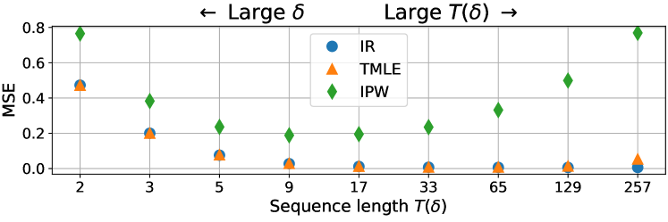
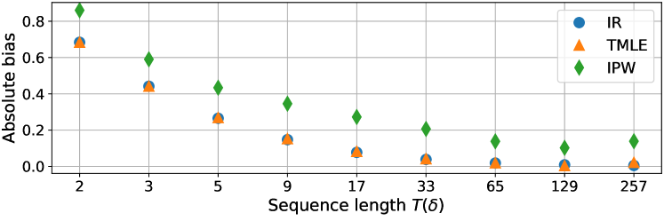
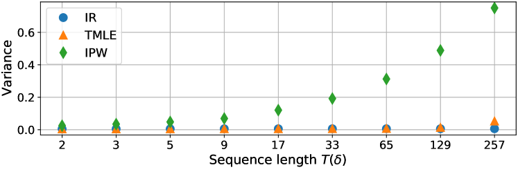
Figure 1: MSE, absolute bias, and variance as a function of sequence length $T(\delta)$ for each estimator. Sequence length $T(\delta)$ was varied by changing the discretization bin width $\delta$ while keeping fixed the sample size (i.e. the total number of participants) and the the number of participants following the treatment regime of interest. The data generating mechanism included both baseline and time-dependent confounding.

The bias, variance, and MSE for each estimator under different $\delta$ are shown in Figure 1. Though somewhat hard to see in the Figure, variance increases with sequence length for all estimators with a sharp increase in variance for the TMLE and IPW estimators on long sequences. This increase is most severe for the IPW estimator, followed by TMLE and then IR, the last of which does not show the same steep increase in variance as the other two. In Section 3 of the supplementary material, we review and evaluate several approaches to reducing this variance.

Additionally, we observe two distinct forms of bias. First, the IPW estimator exhibits increased bias in the longest sequences. This is likely due to finite sample bias caused by near-positivity violations. Specifically, as $\delta$ becomes smaller, the probability of a participant beginning treatment within each time bin grows smaller until, for small enough $\delta$, we observe bins containing no jumps. Consistent with previous studies [18, 33], we observe that these finite sample positivity violations have a much smaller effect on the IR and TMLE methods than the IPW method. In the presence of positivity violations the IR an TMLE methods must extrapolate when estimating $Q$. If the model for $Q$ is a correctly specified parametric model (as it is in this example), this extrapolation may result in relatively little bias; however, due to potential model misspecification, we cannot expect this in general.

We observe a second form of bias when $\delta$ is large and $T(\delta)$ is small. Importantly, for all estimators, this bias occurs even when there is no confounding (see Section 2 of the supplementary material for an example). This second form of bias dominates MSE for large $\delta$, whereas variance dominates MSE for small $\delta$. In the next section, we discuss this second source of bias in the IR and TMLE methods and give recommendations for avoiding it.

6 Discretization bias in IR and TMLE

6.1 Probability limits of estimators using uncoarsened vs. coarsened data

Suppose that we have discretized our data using bin width $\delta^{*}$ and, as in the previous section, we coarsen the finest discretization by using a subset of its time points. We show that if, in the coarsened sequence, changing a treatment value within a discrete time bin can have a causal effect on feature values within the same time bin, then the IR and TMLE estimators applied to the coarsened data may result in inconsistent estimators of $\mathbb{E}[Y^{\bar{a}(\delta^{*})}]$ even under correct model specification and without time-dependent confounding. We further show that this result explains the bias observed in Section 5 when using IR and TMLE with large $\delta$.

Throughout the remainder of this section, all quantities are with respect to the finest discretization, $\delta^{*}$, unless otherwise specified. As in our simulated data experiments, we will assume that the finest discretization satisfies a Markov property with respect to $\bar{L}$ and Y, that is, $L_{t}\perp\!\!\!\perp\bar{L}_{t-2}\mid\bar{A}_{t-1},L_{t-1}$ and $Y\perp\!\!\!\perp\bar{L}_{T^{*}-1}\mid\bar{A}_{T^{*}},L_{T^{*}}$. We will assume that the finest discretization obeys the causal identifiability assumptions, but we will not assume that the coarsened sequence does. For simplicity, we assume that all baseline features are included in $L_{1}$ (so there is no $V$).

As before, consider coarsening this sequence to have bin width $\delta$, where $\delta$ is a multiple of $\delta^{*}$. Denote by $\bar{s}=\{s(1),...,s(T(\delta))\}\subset\{1,...,T^{*}\}$ the subset of indices from the finest discretization included in the coarsened one where $s(k)$ is the $k$’th value in $\bar{s}$. By definition, $\bar{s}$ has length $T(\delta)$ and we assume that the first and last indices of the uncoarsened sequence are included in $\bar{s}$, i.e., $s(1)=1$ and $s(T)=T^{*}$. It follows that $L_{s(k)}=L(\delta)_{k}$ and the same holds replacing $L$ by $A$. Our interest is in the difference between the probability limits of a given estimator when applied to the finest discretization and to the coarsened discretization $\bar{s}$; we separately determine this for the IR and TMLE estimators. Recall that, for any discretization of the data, the IR estimator converges in probability to the g-computation formula applied according to that discretization, as long as the corresponding $Q$ is consistently estimated; this holds as well for the TMLE if either the corresponding $g$ or $Q$ is consistently estimated. We show how the coarsened and uncoarsened g-computation formulas differ and describe conditions under which the two are equal.

For conciseness of notation, we write expressions such as $P(X=x\mid Z=z)$ and $\mathbb{E}[X\mid Z=z]$ as $P(X=x\mid z)$ and $\mathbb{E}[X\mid z]$, respectively. E.g., we write $P(L_{k}=l_{k}\mid\bar{A}_{k-1}=\bar{a}_{k-1},L_{k-1}=l_{k-1})$ as $P(L_{k}=l_{k}\mid\bar{a}_{k-1},l_{k-1})$. Using the Markov assumption and assuming that each $L_{t}$ is discrete valued, the g-computation formula applied to the coarsened sequence can be written as

$$\sum_{\bar{l}(\delta)}\mathbb{E}[Y\mid\bar{a}(\delta),l(\delta)_{T(\delta)}]\prod_{k=1}^{T(\delta)}P(L(\delta)_{k}=l(\delta)_{k}\mid\bar{a}(\delta)_{k-1},l(\delta)_{k-1}),$$ (2)

where the sum over $\bar{l}(\delta)$ indicates a sum over all possible coarsened feature sequences and conditioning on $\bar{a}(\delta)$ indicates conditioning on the coarsened treatment sequence. We now highlight the differences between this quantity and the uncoarsened g-computation formula. Recalling that $\bar{l}_{j:k}=[l_{j},l_{j+1},\dots,l_{k}]$ and that $L_{t}^{\bar{a}_{j:k}}$ is the potential outcome of $L_{t}$ when only the treatment subsequence $\bar{a}_{j:k}$ is set, we can rewrite the uncoarsened g-computation formula as

$$\mathbb{E}\left[Y^{\bar{a}}\right] =\sum_{\bar{l}}\mathbb{E}[Y\mid\bar{a},l_{T^{*}}]\prod_{t=1}^{T^{*}}P(L_{t}=l_{t}\mid\bar{a}_{t-1},l_{t-1})$$ (3)

$$\begin{split}&=\sum_{\bar{l}(\delta)}\mathbb{E}[Y\mid\bar{a},l(\delta)_{T(\delta)}]P(L(\delta)_{1}=l(\delta)_{1})\\ &\qquad\qquad\qquad\qquad\cdot\prod_{k=2}^{T(\delta)}P(L(\delta)^{\bar{a}_{s(k-1)+1:s(k)-1}}_{k}=l(\delta)_{k}\mid\bar{a}_{s(k-1)},l(\delta)_{k-1}),\end{split}$$ (4)

where the sum over $\bar{l}$ in Equation 3 indicates a sum over all possible values of the uncoarsened feature sequence. A complete derivation of Equation 4 is given in Section 4.1 of the supplementary materials. The coarsened (Equation 2) and uncoarsened (Equation 4) g-computation formulas differ in two ways. First, all expressions in Equation 2 condition on the coarsened treatment sequence $\bar{a}(\delta)$, whereas expressions in Equation 4 condition on the uncoarsened treatment sequence $\bar{a}$. Second, in Equation 2 the expected outcome $\mathbb{E}[Y\mid\bar{a}(\delta),l(\delta)_{T}]$ is multiplied by the product of terms $P(L(\delta)_{k}=l(\delta)_{k}\mid\bar{a}(\delta)_{k-1},l(\delta)_{k-1})$, while in Equation 4 the expected outcome is multiplied by the same product but with $L(\delta)_{k}$ replaced by the intervened-on measurement $L(\delta)^{\bar{a}_{s(k-1)+1:s(k)-1}}_{k}$. It follows that if, for all $k$, (i) conditioning on $\bar{a}(\delta)_{k}$ is equivalent to conditioning on $\bar{a}_{s(k)}$ and (ii) the sequence of treatments between times $s(k-1)$ and $s(k)$ (exclusive) does not have a causal effect on the subsequent measurement $L(\delta)_{k}$, then the coarsened and uncoarsened g-computation formulas are equal. Therefore, under conditions (i) and (ii), and under the assumptions necessary to guarantee that IR and TMLE converge in probability to the coarsened g-computation formula — including consistent estimation of $Q$ and/or $g$ — as well as the causal identifiability assumptions for the finest discretization, IR and TMLE applied to the coarsened data converge in probability to the original estimand $\mathbb{E}[Y^{\bar{a}(\delta^{*})}]$. Importantly, conditions (i) and (ii) may be violated even when $\bar{L}$ has no causal effect on $\bar{A}$, which means that coarsening the finest discretization may still induce bias, asymptotically, in IR and TMLE when there is no time-dependent confounding. The binary treatment sequences that we consider in this work satisfy condition (i) when considering $\bar{a}=0$ or $\bar{a}=1$. Additional work is necessary to investigate other types of treatment sequences and settings that do not follow the Markov assumption.

6.2 Discretization bias in simulations

Figure 2: Absolute bias of the IR estimator on data with different effect delays $\omega$ and discretization bin widths $\delta$. Each line corresponds to a different effect delay $\omega$. The $\omega=1$ line corresponds exactly to the absolute bias plot for IR in Figure 1.

We return to the simulated data experiments from Section 5. Note the following: the data generating distribution described in Section 5 satisfies the Markov assumption; for all $\delta$, the “never treat” regime we considered satisfies condition (i) above; the parametric models for $Q_{t}$ are correctly specified for coarsened data; and, the causal identifiability assumptions are satisfied at $\delta^{*}$. Thus, the bias we observe when using IR and TMLE with $\delta>\delta^{*}$ (Figure 1) may be due to violations of condition (ii). We illustrate this point by modifying the data generating mechanism from Section 5 to include an effect delay $\omega$ such that, in the data generating mechanism, $L_{t}$ now depends on $A_{t-\omega}$ rather than $A_{t-1}$ (by convention, $A_{t}=0$ for all $t<1$). All other aspects of the data generating mechanism, estimation methods, and experimental setup remained the same, including the target estimand, $\mathbb{E}[Y^{\bar{a}(\delta^{*})=0}]$. In particular, $\omega=1$ is exactly equivalent to the experimental setup in Section 5. In this new setup, condition (ii) is satisfied for all $\delta\leq\omega$. Figure 2 shows how changing the discretization bin width $\delta$ impacts the bias of the IR estimator under different settings of the effect delay, $\omega$. As predicted by the above analysis, we see that the bias remains near zero as long as $\delta\leq\omega$. For $\delta>\omega$ the bias grows as in Section 5. The same plot for the TMLE estimator is very similar and can be found in Section 4.2 of the supplementary materials. In the next section, we evaluate the impact of $\delta$ in the context of a real clinical causal estimation problem: estimating the effect of antibiotics timing in patients with sepsis.

7 Estimating the effect of delayed versus immediate antibiotics for patients with sepsis

Several observational studies have suggested that delaying the initiation of antibiotics in patients with sepsis leads to poorer health outcomes; however, these studies do not account for potential time-dependent confounding or right censoring. In this section, we use the estimators described in Section 4 to examine the impact of delayed antibiotics on later organ dysfunction, a primary symptom of sepsis. We estimated the average treatment effect (ATE) of receiving antibiotics within one hour of admission versus not receiving antibiotics within the first 13 hours after admission on the number of dysfunctional organ systems 73 hours after admission. Our data included electronic health records from 9,523 patients admitted to the emergency department at one of three hospitals in the Johns Hopkins Hospital system between 2016 and 2018. Patients were included if they were above age 18 and were classified as having sepsis (according to the definition introduced in Henry et al. [6]) with onset occurring within the first 24 hours after admission. The number of dysfunctional organ systems was measured as the sum of the nine organ dysfunction criteria defined in Henry et al. [6]. Summary statistics are shown in Table 1.

Antibiotics initiation was represented as a binary, time-varying treatment. We adjusted for potential time-varying confounding and for right-censoring that occurs when a patient either leaves the hospital against medical advice or is transferred to another critical care facility. If a patient died or was discharged (excluding transfers to critical care facilities) before 73 hours after admission, their outcome was measured as the number of dysfunctional organ systems at the time of death or discharge and such patients were not considered right-censored. If a patient died or was discharged prior to receiving antibiotics, it is assumed that they never subsequently received antibiotics. The complete list of baseline and time-varying features is given in Section 5.1 of the supplementary materials and includes various demographics, comorbidities, lab measurements, and vital signs. All continuous variables were discretized into five quantile bins.

	Full Sample	Abx. $\leq$ 1 hour	Abx. $>$ 13 hours
Number of Participants	9,523	624	1,177
Age	63.30 (17.68)	65.68 (16.82)	61.07 (17.25)
Sex=female	4711 (49.5%)	340 (54.5%)	597 (50.7%)
Charlson Comorbidity Index (CCI)	7.50 (4.01)	7.45 (3.70)	7.65 (4.17)
In-hospital mortality	1126 (11.8%)	106 (17.0%)	174 (14.8%)
No. organ dysfunctions at 13hrs	1.35 (1.31)	1.82 (1.51)	1.22 (1.17)
No. organ dysfunctions at 25hrs	1.26 (1.33)	1.61 (1.49)	1.29 (1.27)
No. organ dysfunctions at 49hrs	1.09 (1.32)	1.38 (1.51)	1.26 (1.39)
No. organ dysfunctions at 73hrs	0.99 (1.31)	1.23 (1.44)	1.21 (1.41)
In-hospital mortality w/in 73hrs	434 (4.6%)	63 (10.1%)	46 (3.9%)
Discharged w/in 73hrs	419 (4.4%)	21 (3.4%)	21 (1.8%)
Censored w/in 73hrs	341 (3.6%)	24 (3.8%)	22 (1.9%)

Table 1: Summary statistics for the Full Sample, patients who received antibiotics within an hour of admission (Abx. $\leq$ 1 hour), and patients who had not received antibiotics in the first 13 hours after admission (Abx. $>$ 13 hour). Binary variables are summarized as the count and (percentage). Continuous variables are summarized as the mean and (standard deviation). Note that the average number of dysfunctional organ systems decreased over time as patients stabilized or recovered. For patients who died or were discharged before time $t$, their number of organ dysfunctions at time $t$ was recorded as the number of organ dysfunctions at the time of death or discharge.

We choose $\delta^{*}=1$ hour as our finest discretization and introduce a binary censoring variable $\bar{C}(\delta^{*})=[C(\delta^{*})_{1},...,C(\delta^{*})_{T^{*}}]$, where $C(\delta^{*})_{t}=1$ indicates that a patient was censored at or before time $t$. The temporal ordering of variables under the finest discretization is assumed to be

$$V,L(\delta^{*})_{1},C(\delta^{*})_{1},A(\delta^{*})_{1},...,L(\delta^{*})_{T},C(\delta^{*})_{T},A(\delta^{*})_{T},Y.$$

For the finest discretization, we make the causal identifiability assumptions and assume that they apply to $\bar{C}(\delta^{*})$ as well as $\bar{A}(\delta^{*})$. Because we are only interested in antibiotics administration before hour 13, we consider static treatment regimes that set the value of treatment through hour 13 and leave treatment after hour 13 unspecified. That is, anyone who does not have antibiotics administered in the first 13 hours (regardless of treatment after hour 13) is following the treatment regime $\bar{a}(\delta^{*})=0$. Likewise, anyone who receives antibiotics in the first hour after admission is following regime $\bar{a}(\delta^{*})=1$. Our target estimand is $\mathbb{E}[Y^{\bar{a}(\delta^{*})=0,\bar{c}(\delta^{*})=0}-Y^{\bar{a}(\delta^{*})=1,\bar{c}(\delta^{*})=0}]$.

We estimated $g$ and $Q$ using modified versions of the parametric models described in Section 5. The parametric model for $g_{t}$ was modified to incorporate the assumption that a patient cannot initiate antibiotics or become newly censored after death or discharge. We used a parametric model of the same form as that used for $g_{t}$ to estimate the probability of becoming newly censored at time $t$. The parametric model for $Q_{t}$ was modified to incorporate the assumption that a patient’s outcome cannot change after death or discharge. Full details for these models are given in Section 5.2 of the supplementary materials. 95% confidence intervals were constructed using percentile-based non-parametric bootstrap using 500 bootstrap replicates.

We compared the performance of the three estimators described in Section 4 using discretization bin widths of $\delta=1$, $3$, and $6$ hours corresponding to sequences with $T(\delta)=73$, $25$, and $13$ time points, respectively. These discretizations always included hours $1$, $13$, and $73$ as time points and thus, changing $\delta$ did not change $\mathbb{E}[Y^{\bar{a}(\delta),\bar{c}(\delta)=0}]$ under the treatment regimes considered. We make causal identifiability assumptions only for bin width $\delta=\delta^{*}=1$ hour.

7.1 Results

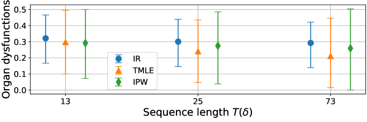
Figure 3: Estimates of the ATE of delayed versus immediate antibiotics on the expected number of dysfunctional organ systems 73 hours after admission. Point estimates and 95% confidence intervals are shown for each estimator and for each sequence length $T(\delta)$.

Figure 3 shows the estimated ATE for each of the three estimators using sequences of length $T(\delta)=13$, $25$, and $73$. Using the finest discretization ($\delta=\delta^{*}=1$ hour), all three estimates of the ATE show that the effect of delayed versus immediate antibiotics was an increase in the number of dysfunctional organ systems at 73 hours. Further, all three estimated 95% confidence intervals exclude zero. In contrast, a naive estimate of the ATE — estimated by taking the difference in average outcomes in the two treatment groups — show a near-zero effect ($-0.01$ $[-0.11\text{ to }0.12]$). We find that, for each of the three estimators, the point estimates are largely consistent across $\delta=1,3,6$. At the finest discretization, the IR method results in the narrowest confidence interval, followed by TMLE, and then by IPW. Confidence interval widths range from 0.28 to 0.30 for IR, from 0.39 to 0.43 for TMLE, and from 0.43 to 0.50 for IPW. In Section 4 of the supplementary material, we evaluate the impact of weight clipping and pooling on these estimates.

8 Discussion

It has become increasingly viable to evaluate hypothetical treatment regimes using non-experimental data thanks to the availability of high-resolution logged data. Before applying discrete-time longitudinal causal estimation methods to these problems, it is necessary to understand how the behavior of these methods is impacted by temporally discretizing the data. We evaluated the impact of discretization bin width on three causal estimation methods, inverse probability weighting (IPW), an iterated regressions method (IR), and a targeted minimum loss-based estimator (TMLE), when estimating an expected potential outcome under a binary treatment sequence with at most a single 0-to-1 transition. These results highlight two main takeaways for those hoping to apply these methods.

First, results from both simulated and clinical data corroborated previous results [10, 32] showing that IR has substantially lower variance in long sequences than IPW, with TMLE somewhere between the two. This latter result is in contrast with a previous comparison of IR and TMLE [33]; however, we found that the variance gap only appeared for relatively long sequences whereas Tran et al. [33] considered sequences up to length six. This suggests that the double-robustness property of TMLE may come at the cost of increased variance in long sequences; however, the size of the variance gap may depend on the application.

Second, we found on simulated data that overly-wide discretization bins led to substantial bias in all three estimators. For IR and TMLE, we explored the source of this bias and found that it is governed, in part, by whether a change in treatment can effect features within the same discretization bin. Our analysis suggests a rule-of-thumb for choosing discretization bin widths when using these estimators: Choose the widest bins such that changing treatment within a bin does not affect features within the same bin. For example, in our application, if we do not believe the effect of antibiotics will be noticeable until at least six hours after administration, this suggests six hours as a plausible bin width. If instead we were to consider the effects of a fast acting medication, this bin width would need to be smaller. When such domain knowledge is unavailable, practitioners should exercise caution when applying discrete-time methods to continuous-time data and should consider continuous-time causal estimation methods. We emphasize this particularly in the case of applications of RL to continuous-time decision making settings where it is standard practice to model the system as a discrete-time time-homogeneous Markov decision process, e.g., [10, 32, 5, 11, 31].

This work highlights the importance of discretization decisions and sequence length in real-time causal estimation settings and suggests several future research directions. First, this work is limited to binary treatment sequences with a single 0-to-1 transition and the results in Sections 5 and 6 are limited by the Markov assumption. Additional work is necessary to investigate scenarios that do not have these limitations. Second, it would be practically useful to develop general diagnostic techniques to guide discretization decisions when domain knowledge is not readily available and, potentially, data driven methods for automatically selecting the bin width to minimize estimation error. Additionally, when continuous-time or high-resolution data is available, it may be possible to quantify or bound the amount of discretization bias under certain assumptions. Finally, given the observed sensitivity of these methods to bin width, it is important to continue development of continuous-time methods that obviate the need for discretization in settings with insufficient domain knowledge to guide bin width decisions.

Appendix A Complete descriptions of IR and TMLE

A.1 Iterative regression (IR)

The IR algorithm iteratively estimates each $Q_{t}$, beginning with $Q_{T}$ and progressing backwards in time. The full algorithm is described below.

1. Estimate the conditional expectation $Q_{T}=\mathbb{E}[Y|\bar{A}_{T}=\bar{a}_{T},\bar{L}_{T},V]$ by regressing $Y$ onto $(\bar{L}_{T},V)$ using data from participants who followed $\bar{a}$ through time $T$. For each participant $i$ who followed $\bar{a}$ through time $T-1$, let $\hat{Q}_{i,T}$ be this estimate evaluated at $(\bar{L}_{i,T},V_{i})$.

2. For $t=T-1,...,1$:

   1. Estimate the conditional expectation $Q_{t}=\mathbb{E}[Q_{t+1}|\bar{A}_{t}=\bar{a}_{t},\bar{L}_{t},V]$ by regressing the values $\hat{Q}_{t+1}$ (calculated in the previous iteration) onto $(\bar{L}_{t},V)$ using data from participants who followed $\bar{a}$ through time $t$. For each participant $i$ who followed $\bar{a}$ through time $t-1$, let $\hat{Q}_{i,t}$ be this estimate evaluated at $(\bar{L}_{i,t},V_{i})$.

3. Return $\hat{\psi}_{IR}=\frac{1}{N}\sum_{i}\hat{Q}_{i,1}$.

A.2 Targeted minimum loss-based estimation (TMLE)

The TMLE algorithm modifies the IR algorithm to add an additional targeting step, which updates the initial estimate of $Q_{t}$ using the probability of treatment $g$ as detailed below.

1. Estimate the probability of treatment $\hat{g}$ as in Section 4.1 of the main paper.

2. Estimate the conditional expectation $Q_{T}=\mathbb{E}[Y|\bar{A}_{T}=\bar{a}_{T},\bar{L}_{T},V]$ by regressing $Y$ onto $(\bar{L}_{T},V)$ using data from participants who followed $\bar{a}$ through time $T$. For each participant $i$ who followed $\bar{a}$ through time $T-1$, let $\hat{Q}_{i,T}$ be this estimate evaluated at $(\bar{L}_{i,T},V_{i})$.

3. Regress $Y$ onto an intercept with $\hat{Q}_{T}$ as a fixed offset and $\frac{\mathbb{I}[\bar{A}_{T}=\bar{a}_{T}]}{\hat{g}(\bar{a};\bar{L}_{T},V)}$ as observation weights using data from participants who followed $\bar{a}$ through time $T$. For each participant $i$ who followed $\bar{a}$ through time $T-1$, let $\hat{Q}^{*}_{i,T}$ be this fitted regression evaluated with offset $\hat{Q}_{i,T}$.

4. For $t=T-1,...,1$:

   1. Estimate the conditional expectation $Q_{t}=\mathbb{E}[Q_{t+1}|\bar{A}_{t}=\bar{a}_{t},\bar{L}_{t},V]$ by regressing $\hat{Q}^{*}_{t+1}$ (calculated in the previous iteration) onto $(\bar{L}_{t},V)$ using data from participants who followed $\bar{a}$ through time $t$. For each participant $i$ who followed $\bar{a}$ through time $t-1$, let $\hat{Q}_{i,t}$ be this estimate evaluated at $(\bar{L}_{i,t},V_{i})$.

   2. Regress $\hat{Q}^{*}_{t+1}$ onto an intercept with $\hat{Q}_{t}$ as a fixed offset and $\frac{\mathbb{I}[\bar{A}_{t}=\bar{a}_{t}]}{\hat{g}(\bar{a}_{t};\bar{L}_{t},V)}$ as observation weights using data from participants who followed $\bar{a}$ through time $T$. For each participant $i$ who followed $\bar{a}$ through time $t-1$, let $\hat{Q}^{*}_{i,t}$ be this fitted regression evaluated with offset $\hat{Q}_{i,t}$.

5. Return $\hat{\psi}_{TMLE}=\frac{1}{N}\sum_{i}\hat{Q}^{*}_{i,1}$.

Appendix B Simulated RCT

In this section, we compare the estimators presented in Section 4 of the main paper using a modified version of the data generating mechanism from Section 5 of the main paper where $A_{t}$ is sampled without confounding (i.e., $\bm{\gamma}_{1}=\mathbf{0}$ and $\bm{\gamma}_{2}=\mathbf{0}$). This simulates a randomized trial where subjects are assigned a random treatment start time. All other details of the data generating mechanism, experimental setup, and estimation procedures remained the same. Results are shown in Figure 4. Of note, for large $\delta$, we observe increased bias for all estimators, despite the lack of confounding.

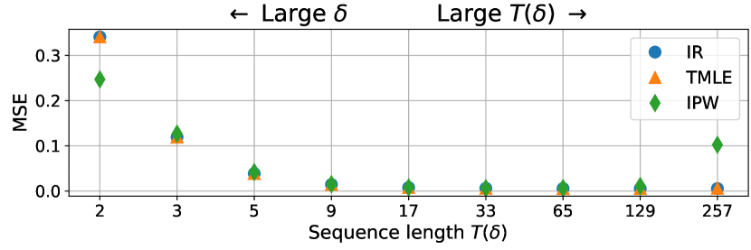
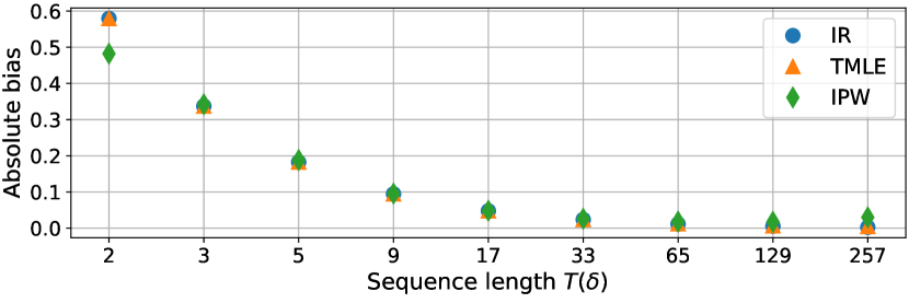
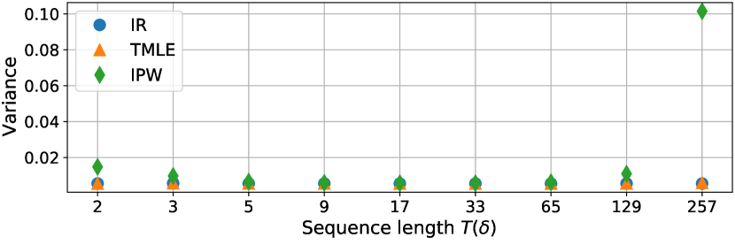
Figure 4: MSE, absolute bias, and variance as a function of sequence length $T(\delta)$ for each estimator with no baseline of time-dependent confounding. Sequence length $T(\delta)$ was varied by changing the discretization bin width $\delta$ while keeping fixed the sample size (i.e. the total number of participants) and the the number of participants following the treatment regime of interest.

Appendix C Variance reduction strategies

In this section, we consider the impact of three approaches — weight clipping, pooling across treatment regimes, and pooling across time points — to reduce estimator variance in our simulated data experiments from Section 5. We begin by introducing these approaches and describing how they change our experimental setup. Other than the changes described below, no changes were made to the data generating mechanism, assumptions, or estimation procedures described in Section 5 of the main paper.

C.1 Weight clipping

One simple, yet effective method for reducing the variance of estimators based on inverse probability weighting is to clip the weights so that they fall within a prespecified range [2, 12]. This method prevents small sets of instances from dominating the estimate, thereby reducing variance, but may introduce additional bias. In our evaluation, we consider a percentile based clipping where, for a prespecified percentile $\alpha$, the weights $\frac{1}{\hat{g}(\bar{a},\bar{L}_{i},V_{i})}$ among participants who followed $\bar{a}$ are clipped to be between the $\alpha$ and $100-\alpha$ percentiles of the empirical distribution of weights among participants who followed $\bar{a}$.

C.2 Pooling

Another approach to reducing variance is to pool data when estimating $g$ and $Q$. We consider two types of pooling. First, we consider pooling data from multiple treatment regimes when estimating $Q$ [17, 33]. Specifically, to estimate $Q_{t}=\mathbb{E}[Q_{t+1}\mid\bar{A}_{t}=\bar{a}_{t},\bar{L}_{t},V]$ in the IR procedure, we instead estimate $\mathbb{E}[Q_{t+1}\mid\bar{A}_{t},\bar{L}_{t},V]$ using data from all participants. Then, for participants who followed $\bar{a}$ through time $t-1$, we set $\hat{Q}_{i,t}$ to this estimate evaluated at $(\bar{a}_{t},\bar{L}_{i,t},V_{i})$. This same modification can also be made to the initial untargeted estimate of $Q_{t}$ in the TMLE procedure. In our simulated data experiments, this means modifying the the parametric model for $Q_{t}$ to be

$$q_{t}(\bar{A}_{t},\bar{L}_{t},V;\bm{\nu})=\nu_{t,0}+\bm{\nu}_{t,1}L_{t}+\bm{\nu}_{t,2}V+\bm{\nu}_{t,3}\bar{A}_{t}.$$ (5)

where $\bm{\nu}_{t}$ is estimated using data from all participants. Second, we consider pooling across time points when estimating $g$ [8, 7]. This means modifying our model for $g_{t}=P(A_{t}=1\mid A_{t-1}=0,\bar{L}_{t},V)$ to be

$$m_{t}(\bar{L}_{t},V;\bm{\theta})=expit(\theta_{0}+\bm{\theta}_{1}V+\bm{\theta}_{2}L_{t}).$$ (6)

where $\bm{\theta}$ is estimated using data from all participants $i$ and all time points $t$ such that $A_{i,t-1}=0$.

C.3 Results

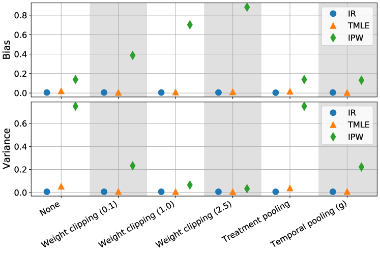
Figure 5: Absolute bias and variance for IPW, IR, and TMLE when using each of the variance reduction methods on synthetic data. We evaluated percentile-based weight clipping with percentiles $\alpha=0.1,1.0,2.5$.

We compared the effect of each of these variance reduction methods using the same data generating distribution and experimental setup (aside from the modifications described above) as in Section 5 of the main paper with a discretization bin width of $\delta=\delta^{*}=1$. Figure 5 shows the impact on absolute bias and variance of each of the variance reduction approaches. Both weight clipping and temporal pooling were extremely effective at reducing variance in the IPW and TMLE methods. In the case of IPW, weight clipping increased bias, as expected. Pooling across treatment regimes, on the other hand, had little observable effect on either the bias or variance of any of the estimators.

Appendix D Supplemental material for Section 6 of the main paper

D.1 Derivation of Equation 4 in the main paper

As in Section 6 of the main paper, all quantities are with respect to the finest discretization, $\delta^{*}$, unless otherwise specified. Then, recalling that $\bar{l}_{j:k}=[l_{j},l_{j+1},\dots,l_{k}]$ and that $L_{t}^{\bar{a}_{j:k}}$ is the potential outcome of $L_{t}$ when only the treatment subsequence $\bar{a}_{j:k}$ is set, we can rewrite the uncoarsened g-computation formula as

$$\mathbb{E}[Y^{\bar{a}}] =\sum_{\bar{l}}\mathbb{E}[Y\mid\bar{a},l_{T^{*}}]\prod_{t=1}^{T^{*}}P(L_{t}=l_{t}\mid\bar{a}_{t-1},l_{t-1})$$ (7)

$$\begin{split}&=\sum_{\bar{l}(\delta)}\sum_{\bar{l}_{s(1)+1:s(2)-1}}\dots\sum_{\bar{l}_{s(T-1)+1:s(T)-1}}\mathbb{E}[Y\mid\bar{a},l_{T^{*}}]P(L_{1}=l_{1})\\ &\mspace{270.0mu}\cdot\prod_{k=2}^{T(\delta)}\left\{\prod_{t=s(k-1)+1}^{s(k)}P(L_{t}=l_{t}\mid\bar{a}_{t-1},l_{t-1})\right\}\end{split}$$ (8)

$$=\sum_{\bar{l}(\delta)}\mathbb{E}[Y\mid\bar{a},l_{T^{*}}]P(L_{1}=l_{1})\prod_{k=2}^{T(\delta)}\,\,\sum_{\bar{l}_{s(k-1)+1:s(k)-1}}\left\{\prod_{t=s(k-1)+1}^{s(k)}P(L_{t}=l_{t}\mid\bar{a}_{t-1},l_{t-1})\right\}$$ (9)

$$=\sum_{\bar{l}(\delta)}\mathbb{E}[Y\mid\bar{a},l_{T^{*}}]P(L_{1}=l_{1})\prod_{k=2}^{T(\delta)}P(L^{\bar{a}_{s(k-1)+1:s(k)-1}}_{s(k)}=l_{s(k)}\mid\bar{a}_{s(k-1)},l_{s(k-1)})$$ (10)

$$\begin{split}&=\sum_{\bar{l}(\delta)}\mathbb{E}[Y\mid\bar{a},l(\delta)_{T(\delta)}]P(L(\delta)_{1}=l(\delta)_{1})\\ &\qquad\qquad\qquad\qquad\cdot\prod_{k=2}^{T(\delta)}P(L(\delta)^{\bar{a}_{s(k-1)+1:s(k)-1}}_{k}=l(\delta)_{k}\mid\bar{a}_{s(k-1)},l(\delta)_{k-1}),\end{split}$$ (11)

where the sum over $\bar{l}$ in Equation 7 indicates a sum over all possible values of the uncoarsened feature sequence; Equation 8 partitions the sum over $\bar{l}$ into the sum over the components in $\bar{l}(\delta)$ (i.e., those in the coarsened sequence: $s(1),\dots,s(T(\delta))$) and over the remaining components; Equation 9 follows from factorizing the nested sums in Equation 8 and the assumption that $s(1)=1$ and $s(T(\delta))=T^{*}$; Equation 10 follows by recognizing that (by the Markov assumption) the inner sum in Equation 9 is an instance of the g-computation formula applied to “outcome” $\mathbb{I}[L_{s(k)}=l_{s(k)}]$ setting treatments at each time $s(k-1)+1$ through $s(k)-1$ and conditioning on the (uncoarsened) history through $s(k-1)$; and Equation 11 follows from the observation that $L_{s(k)}=L(\delta)_{k}$.

D.2 Effect delay in the TMLE model

Figure 6 shows the impact of changing the effect delay $\omega$ on the absolute bias of the TMLE estimator for different bin widths $\delta$. See Section 6 of the main paper for experimental details.

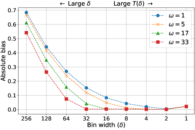
Figure 6: Absolute bias of the TMLE estimator on data with different effect delays. Each line corresponds to different discretizations of data with the same effect delay. The $\omega=1$ line corresponds exactly to the absolute bias plot for the TMLE estimator in Figure 1 of the main paper.

Appendix E Supplemental material for Section 7 of the main paper

E.1 List of features

As baseline features, we included age, sex, Charlson Comorbidity Index (CCI), hospital ID, and indicators for comorbidities measured using billing codes including diabetes without complications, diabetes with complications, malignant tumor, and metastatic solid tumor. As time-varying features, we included indicators of death or discharge, temperature, systolic blood pressure, white blood cell count, lactate, mean arterial pressure (MAP), heart rate, respiration rate, Glasgow Coma Scale (GCS), weight, indicators for the presence of measurements of each of the preceding labs/vitals, and indicators for presence of stroke, seizure, dementia, fall, gastro-intestinal (GI) bleeding, cardiac arrest, sickle cell anemia, and drug overdose. Finally, we included as time-varying features indicators of the nine organ dysfunctions from [6] which were summed to measure total organ dysfunction.

E.2 Details for the parametric models used to estimate $g$ and $Q$

The model for $g_{t}$ was modified from the model in Section 5 of the main paper to incorporate the assumption that a patient cannot initiate antibiotics or become newly censored after death or discharge. Let $D_{t}$ be a binary time-varying feature indicating if a patient has died or been discharged prior to time $t$. As described above, $D_{t}$ is included in $L_{t}$. Then, we estimated $g_{t}$ using the following parametric model

$$m_{t}(\bar{L}_{t},V;\bm{\theta}_{t})=\begin{cases}expit(\theta_{t,0}+\bm{\theta}_{t,1}V+\bm{\theta}_{t,2}L_{t})&\text{if $D_{t}=0$}\\ 1&\text{if $D_{t}=1$},\end{cases}$$ (12)

where $\theta_{t}$ was estimated using data from patients who had not died, been discharged, become censored, or received antibiotics by time $t$. We used a parametric model of the same form as $m_{t}$ to estimate the probability of becoming newly censored at time $t$. The parametric model for $Q_{t}$ was modified from the model presented in Section 5 of the main paper to incorporate the assumption that a patient’s outcome cannot change after death or discharge. We estimated $Q_{t}$ using the following parametric model

$$q_{t}(\bar{L}_{t},V;\bm{\nu}_{t})=\begin{cases}\nu_{t,0}+\bm{\nu}_{t,1}L_{t}+\bm{\nu}_{t,2}V&\text{if $D_{t}=0$}\\ Y&\text{if $D_{t}=1$},\end{cases}$$ (13)

where $\bm{\nu}_{t}$ was estimated using data from patients who followed $\bar{a}$ through time $t$ and had not died, been discharged, or become censored by time $t$.

E.3 Variance reduction strategies in clinical data

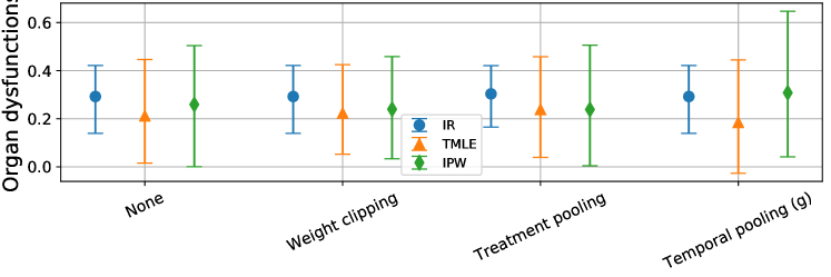
Figure 7: Effects of variance reduction techniques on the real data. Point estimates and $95\%$ confidence intervals are shown for each estimator and each variance reduction technique.

In this section, we evaluate the impact of each of each of the variance reduction approaches described in Section C of the supplementary materials on the clinical decision making problem described in Section 7 of the main paper. For each estimator and variance reduction method, we estimated the ATE and 95 % confidence interval using a discretization bin with of $\delta=\delta^{*}=1$ hour. For the weight clipping method, we used $\alpha=0.1$. All other experimental and estimation details were exactly the same as in Section 7 of the main paper. Figure 7 shows the point estimates and 95% confidence intervals when each of the variance reduction methods is applied. In general, these variance reduction methods had much less of an effect in a real data setting than they did on simulated data. Weight clipping had the largest effect on confidence interval width for the IPW and TMLE estimators, reducing them both from $0.50$ to $0.41$ and $0.40$ to $0.36$, respectively, without a major shift in the point estimates. Additionally, treatment pooling, led to a small reduction in confidence interval width, from $0.28$ to $0.26$, for the IR estimator. Unlike in the simulated data, temporal pooling, led to an increase in confidence interval width for the IPW estimator, as well as a shift in the point estimates for both IPW and TMLE (the shift in the point estimates for the individual expected potential outcomes was even more pronounced). This is possibly due to observable shifts in antibiotics administration behavior over time which violates the assumptions made when pooling across time.

References

- Bang and Robins [2005] Heejung Bang and James M Robins. Doubly robust estimation in missing data and causal inference models. Biometrics, 61(4):962–973, 2005.
- Cole and Hernán [2008] Stephen R Cole and Miguel A Hernán. Constructing inverse probability weights for marginal structural models. American journal of epidemiology, 168(6):656–664, 2008.
- Ferrer et al. [2014] Ricard Ferrer, Ignacio Martin-Loeches, Gary Phillips, Tiffany M Osborn, Sean Townsend, R Phillip Dellinger, Antonio Artigas, Christa Schorr, and Mitchell M Levy. Empiric antibiotic treatment reduces mortality in severe sepsis and septic shock from the first hour: results from a guideline-based performance improvement program. Critical care medicine, 42(8):1749–1755, 2014.
- Glynn [1994] Peter W Glynn. Importance sampling for markov chains: Asymptotics for the variance. Stochastic Models, 10(4):701–717, 1994.
- Gottesman et al. [2018] Omer Gottesman, Fredrik Johansson, Joshua Meier, Jack Dent, Donghun Lee, Srivatsan Srinivasan, Linying Zhang, Yi Ding, David Wihl, Xuefeng Peng, et al. Evaluating reinforcement learning algorithms in observational health settings. arXiv preprint arXiv:1805.12298, 2018.
- Henry et al. [2019] Katharine E Henry, David N Hager, Tiffany M Osborn, Albert W Wu, and Suchi Saria. Comparison of automated sepsis identification methods and electronic health record–based sepsis phenotyping: Improving case identification accuracy by accounting for confounding comorbid conditions. Critical care explorations, 1(10), 2019.
- Hernan and Robins [2020] Miguel A Hernan and James M Robins. Causal Inference: What If. Boca Raton: Chapman & Hall/CRC, 2020.
- Hernán et al. [2000] Miguel Ángel Hernán, Babette Brumback, and James M Robins. Marginal structural models to estimate the causal effect of zidovudine on the survival of hiv-positive men. Epidemiology, pages 561–570, 2000.
- Horvitz and Thompson [1952] Daniel G Horvitz and Donovan J Thompson. A generalization of sampling without replacement from a finite universe. Journal of the American statistical Association, 47(260):663–685, 1952.
- Jiang and Li [2016] Nan Jiang and Lihong Li. Doubly robust off-policy value evaluation for reinforcement learning. In International Conference on Machine Learning, pages 652–661. PMLR, 2016.
- Komorowski et al. [2018] Matthieu Komorowski, Leo A Celi, Omar Badawi, Anthony C Gordon, and A Aldo Faisal. The artificial intelligence clinician learns optimal treatment strategies for sepsis in intensive care. Nature medicine, 24(11):1716–1720, 2018.
- Lee et al. [2011] Brian K Lee, Justin Lessler, and Elizabeth A Stuart. Weight trimming and propensity score weighting. PloS one, 6(3):e18174, 2011.
- Lim [2018] Bryan Lim. Forecasting treatment responses over time using recurrent marginal structural networks. In Advances in Neural Information Processing Systems, pages 7483–7493, 2018.
- Liu et al. [2017] Vincent X Liu, Vikram Fielding-Singh, John D Greene, Jennifer M Baker, Theodore J Iwashyna, Jay Bhattacharya, and Gabriel J Escobar. The timing of early antibiotics and hospital mortality in sepsis. American journal of respiratory and critical care medicine, 196(7):856–863, 2017.
- Neugebauer et al. [2014] Romain Neugebauer, Julie A Schmittdiel, and Mark J van der Laan. Targeted learning in real-world comparative effectiveness research with time-varying interventions. Statistics in medicine, 33(14):2480–2520, 2014.
- Peltan et al. [2019] Ithan D Peltan, Samuel M Brown, Joseph R Bledsoe, Jeffrey Sorensen, Matthew H Samore, Todd L Allen, and Catherine L Hough. Ed door-to-antibiotic time and long-term mortality in sepsis. Chest, 155(5):938–946, 2019.
- Petersen et al. [2014] Maya Petersen, Joshua Schwab, Susan Gruber, Nello Blaser, Michael Schomaker, and Mark van der Laan. Targeted maximum likelihood estimation for dynamic and static longitudinal marginal structural working models. Journal of causal inference, 2(2):147–185, 2014.
- Petersen et al. [2012] Maya L Petersen, Kristin E Porter, Susan Gruber, Yue Wang, and Mark J Van Der Laan. Diagnosing and responding to violations in the positivity assumption. Statistical methods in medical research, 21(1):31–54, 2012.
- Precup [2000] Doina Precup. Eligibility traces for off-policy policy evaluation. Computer Science Department Faculty Publication Series, page 80, 2000.
- Rhee et al. [2019] Chanu Rhee, Travis M Jones, Yasir Hamad, Anupam Pande, Jack Varon, Cara O’Brien, Deverick J Anderson, David K Warren, Raymund B Dantes, Lauren Epstein, et al. Prevalence, underlying causes, and preventability of sepsis-associated mortality in us acute care hospitals. JAMA network open, 2(2):e187571–e187571, 2019.
- Robins [1986] James Robins. A new approach to causal inference in mortality studies with a sustained exposure period—application to control of the healthy worker survivor effect. Mathematical modelling, 7(9-12):1393–1512, 1986.
- Robins et al. [2008] James Robins, Liliana Orellana, and Andrea Rotnitzky. Estimation and extrapolation of optimal treatment and testing strategies. Statistics in Medicine, 27(23):4678–4721, 2008. doi: https://doi.org/10.1002/sim.3301. URL https://onlinelibrary.wiley.com/doi/abs/10.1002/sim.3301.
- Robins [2000a] James M Robins. Robust estimation in sequentially ignorable missing data and causal inference models. In Proceedings of the American Statistical Association, volume 1999, pages 6–10, 2000a.
- Robins [2000b] James M Robins. Marginal structural models versus structural nested models as tools for causal inference. In Statistical models in epidemiology, the environment, and clinical trials, pages 95–133. Springer, 2000b.
- Robins [2004] James M Robins. Optimal structural nested models for optimal sequential decisions. In Proceedings of the second seattle Symposium in Biostatistics, pages 189–326. Springer, 2004.
- Robins and Rotnitzky [1992] J.M. Robins and A. Rotnitzky. Recovery of information and adjustment for dependent censoring using surrogate markers. In AIDS Epidemiology, Methodological issues. Bikhäuser, 1992.
- Schulam and Saria [2017] Peter Schulam and Suchi Saria. Reliable decision support using counterfactual models. In Advances in Neural Information Processing Systems, pages 1697–1708, 2017.
- Schulam and Saria [2018] Peter Schulam and Suchi Saria. Discretizing logged interaction data biases learning for decision-making. arXiv preprint arXiv:1810.03025, 2018.
- Sofrygin et al. [2019] Oleg Sofrygin, Zheng Zhu, Julie A Schmittdiel, Alyce S Adams, Richard W Grant, Mark J van der Laan, and Romain Neugebauer. Targeted learning with daily ehr data. Statistics in medicine, 38(16):3073–3090, 2019.
- Soleimani et al. [2017] Hossein Soleimani, Adarsh Subbaswamy, and Suchi Saria. Treatment-response models for counterfactual reasoning with continuous-time, continuous-valued interventions. In 33rd Conference on Uncertainty in Artificial Intelligence, UAI 2017. AUAI Press Corvallis, 2017.
- Sutton and Barto [2018] Richard S Sutton and Andrew G Barto. Reinforcement learning: An introduction. MIT press, 2018.
- Thomas and Brunskill [2016] Philip Thomas and Emma Brunskill. Data-efficient off-policy policy evaluation for reinforcement learning. In International Conference on Machine Learning, pages 2139–2148, 2016.
- Tran et al. [2019] Linh Tran, Constantin Yiannoutsos, Kara Wools-Kaloustian, Abraham Siika, Mark Van Der Laan, and Maya Petersen. Double robust efficient estimators of longitudinal treatment effects: comparative performance in simulations and a case study. The international journal of biostatistics, 15(2), 2019.
- van der Laan and Gruber [2012] Mark J. van der Laan and Susan Gruber. Targeted minimum loss based estimation of causal effects of multiple time point interventions. The International Journal of Biostatistics, 8(1):Article 9, 2012. doi: 10.1515/1557-4679.1370. URL http://ideas.repec.org/a/bpj/ijbist/v8y2012i1n9.html.
- van der Laan and Rubin [2006] Mark J van der Laan and Daniel Rubin. Targeted maximum likelihood learning. The International Journal of Biostatistics, 2(1), 2006.