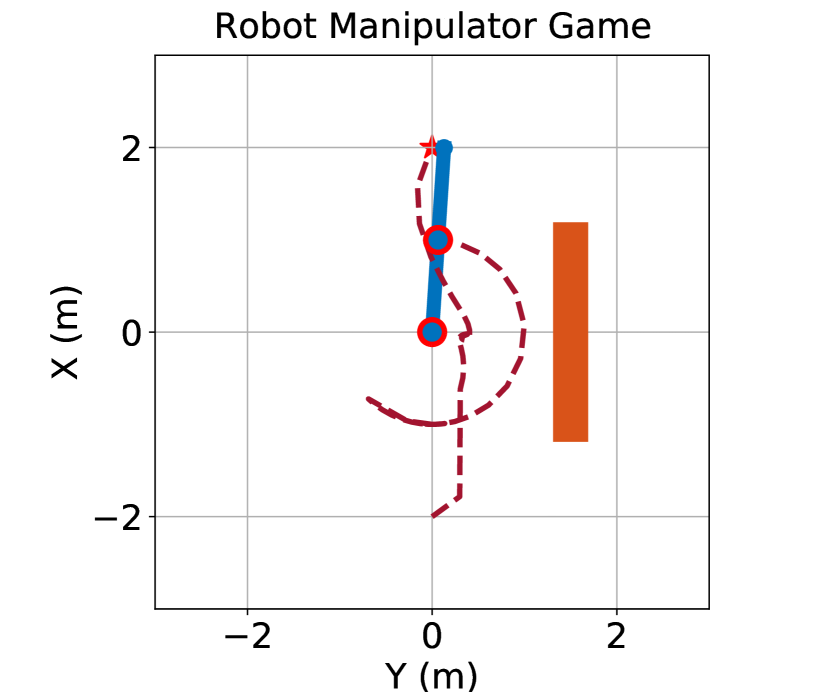
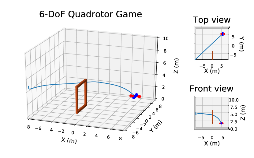
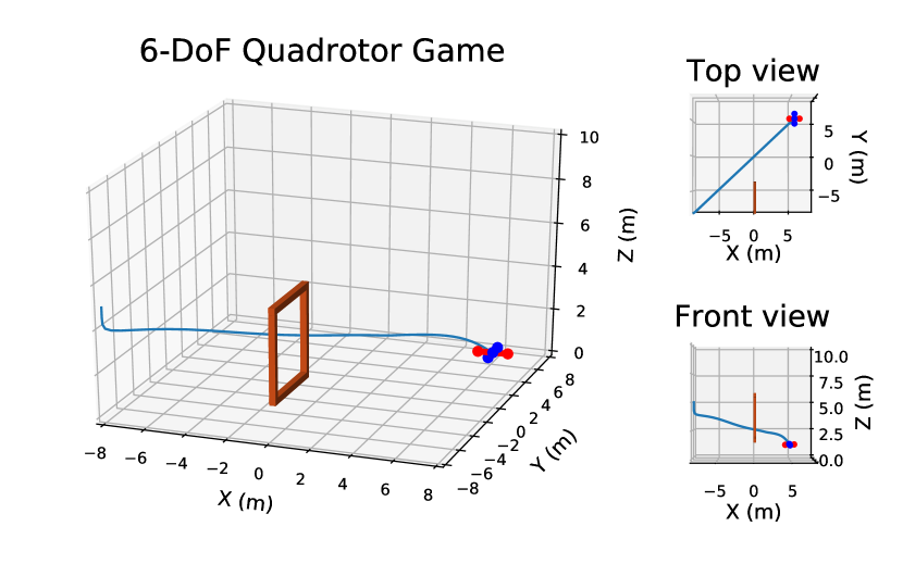
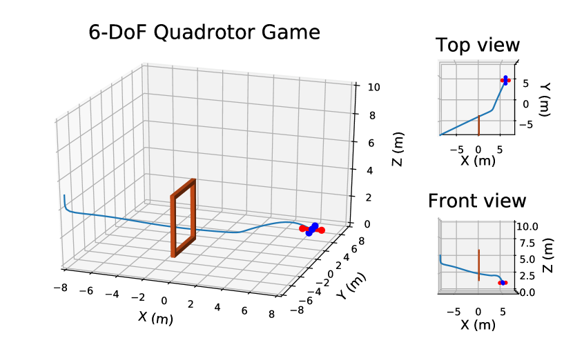
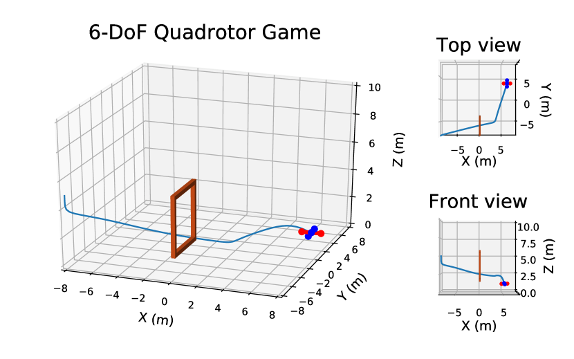
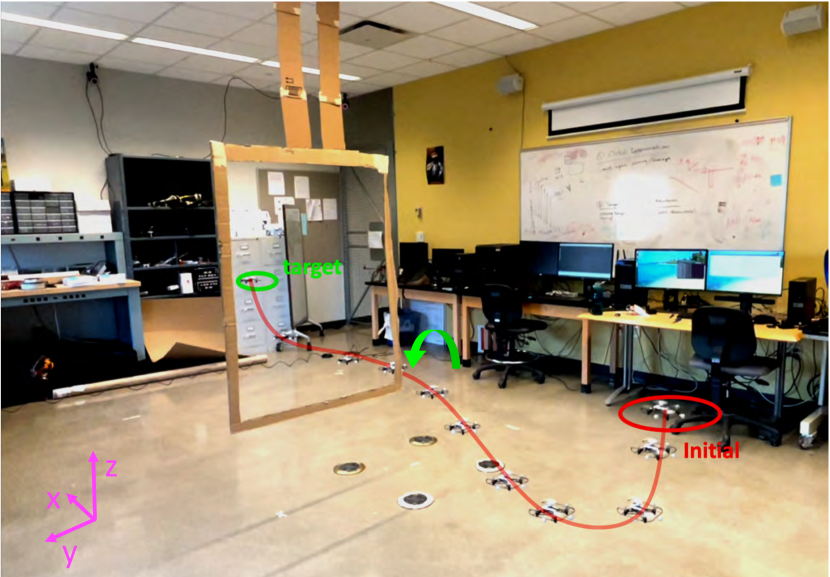
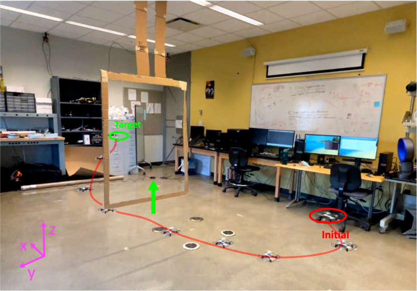
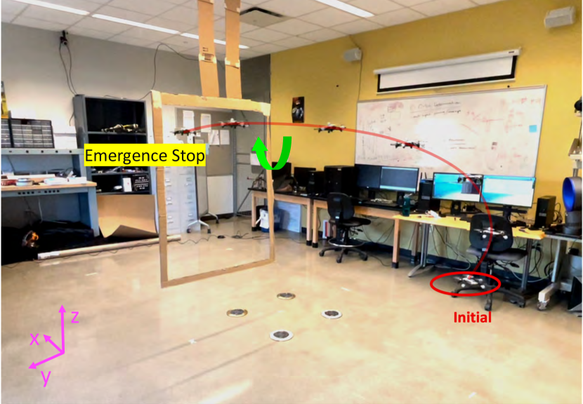
Learning from Human Directional Corrections

Wanxin Jin, Todd D. Murphey, Zehui Lu, Shaoshuai Mou Wanxin Jin is with the General Robotics, Automation, Sensing and Perception (GRASP) Laboratory, University of Pennsylvania, PA 19104, USA. Wanxin Jin is the corresponding author. Email: wanxinjin@gmail.com. Todd D. Murphey is with the Department of Mechanical Engineering, Northwestern University, Evanston, IL 60208, USA. This material is partially based upon work supported by the National Science Foundation under award 1837515. Email: t-murphey@northwestern.edu. Zehui Lu and Shaoshuai Mou are with the School of Aeronautics and Astronautics, Purdue University, West Lafayette, IN 47906, USA. Dr. Mou’s research is supported in part by grants from the Research in Applications for Learning Machines (REALM) Consortium of Northrop Grumman Corporation, Rolls-Royce Corporation, and the NASA University Leadership Initiative (ULI). Email: zehuilu789@gmail.com, mous@purdue.edu. This work involved human subjects or animals in its research. Approval of all ethical and experimental procedures and protocols was granted by Purdue’s Institutional Review Board under Application No. IRB-2021-1539, and performed in the line with Title 45 of the Code of Federal Regulations, Part 46 (45CFR 46).
Abstract

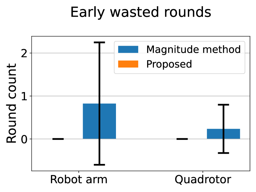
This paper proposes a novel approach that enables a robot to learn an objective function incrementally from human directional corrections. Existing methods learn from human magnitude corrections; since a human needs to carefully choose the magnitude of each correction, those methods can easily lead to over-corrections and learning inefficiency. The proposed method only requires human directional corrections — corrections that only indicate the direction of an input change without indicating its magnitude. We only assume that each correction, regardless of its magnitude, points in a direction that improves the robot’s current motion relative to an unknown objective function. The allowable corrections satisfying this assumption account for half of the input space, as opposed to the magnitude corrections which have to lie in a shrinking level set. For each directional correction, the proposed method updates the estimate of the objective function based on a cutting plane method, which has a geometric interpretation. We have established theoretical results to show the convergence of the learning process. The proposed method has been tested in numerical examples, a user study on two human-robot games, and a real-world quadrotor experiment. The results confirm the convergence of the proposed method and further show that the method is significantly more effective (higher success rate), efficient/effortless (less human corrections needed), and potentially more accessible (fewer early wasted trials) than the state-of-the-art robot learning frameworks.

Index Terms:
Learning from corrections, human-robot physical interaction, motion planning, cutting-plane method, inverse reinforcement learning, learning from demonstrations.

I Introduction

For tasks where robots work in proximity to human users, a robot is required to not only guarantee the accomplishment of the task but also complete it in a way that a human user prefers. Different users may have different preferences about how the robot should perform the task. Such customized requirements usually lead to a considerable workload of robot programming, which requires human users to have high expertise and skills.

To circumvent the above limitations of robot programming, learning from demonstrations (LfD) empowers non-expert users to program robots by providing demonstrations. In LfD [1], a user first provides a robot with demonstrations in a one-time manner, then the robot learns a control policy or objective function offline from the demonstrations. While achieving the notable success in various applications [2, 3, 4], the one-time and offline nature of LfD could lead to some challenges. For example, when the demonstration data is insufficient to infer an objective function due to the low informativeness [5] or deviation from optima [6], the demonstrations have to be re-collected and the robot has to be re-trained. This is particularly inconvenient for robots with high degrees of freedom.

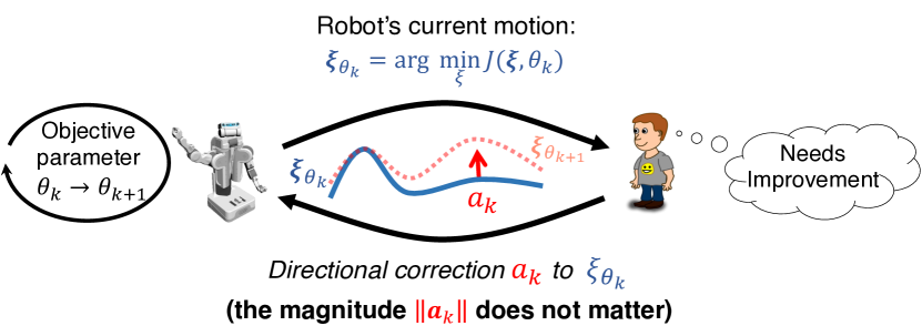
A recent line of work [6, 7, 8, 9] addresses the above challenges of LfD by developing a scheme that enables a robot to learn an objective function from user’s feedback or corrections. Fig. 1 is an example of those learning schemes. At each iteration, a human user does not need to provide optimal demonstrations to the robot, but merely a correction which is an incremental improvement to the robot’s current motion. The robot then leverages the correction to update its objective function. Compared to LfD, this incremental learning scheme reduces the workload of a user, especially for those (such as novices) who cannot provide the optimal demonstrations in a one-time manner [10]. Despite its promise, the state-of-the-art methods [6, 7, 8, 9] still face some challenges as below.
Refer to caption
Figure 1: An illustration of learning from directional corrections proposed in this paper. The robot’s current motion 𝝃𝜽ksubscript𝝃subscript𝜽𝑘\boldsymbol{\xi}_{\boldsymbol{\theta}_{k}} optimizes an objective function parameterized by 𝜽ksubscript𝜽𝑘\boldsymbol{\theta}_{k}. A human user applies a directional correction 𝒂ksubscript𝒂𝑘{\boldsymbol{a}_{k}} to 𝝃𝜽ksubscript𝝃subscript𝜽𝑘\boldsymbol{\xi}_{\boldsymbol{\theta}_{k}}. Note that the magnitude 𝒂kdelimited-∥∥subscript𝒂𝑘\lVert\boldsymbol{a}_{k}\rVert of this correction does not matter. After receiving 𝒂ksubscript𝒂𝑘\boldsymbol{a}_{k}, the robot updates its objective function parameter to 𝜽k+1subscript𝜽𝑘1\boldsymbol{\theta}_{k+1}. This motion-correction-update process repeats until the convergence of the objective function parameter.

First, providing a valid correction—the one that improves the robot motion—can be nontrivial. To obtain a valid correction, the human user must carefully choose the magnitude of a correction. As a robot gets closer to the ‘desired motion’ (i.e., the motion in the human’s perspective), the allowable range of the magnitude of valid corrections gets smaller (see Section II for the detailed explanation). Thus, the human can easily over-correct a robot near the desired motion, i.e., giving too large corrections that adversely drive the robot away from the desired motion. Such difficulty makes robot learning inefficient (we will experimentally show this in Sections V-C and VI).

Second, most of existing methods [7, 8, 9] lack theoretical guarantee for the learning performance. While [6] shows that learning from human magnitude corrections can attain a bounded regret [11], this regret bound still cannot explicitly tell whether or not the learned objective function converges to the true one induced by all corrections.

To address the above challenges, this paper proposes a new learning method that enables a robot to learn an objective function from human directional corrections with theoretical convergence guarantee. We highlight the following new features of the proposed method, as shown by Fig. 1.

(I) The proposed learning scheme only requires the user’s directional corrections. A directional correction is a correction that only concerns directional information and does not necessarily need to be magnitude-specific. For instance, in teaching a mobile robot, a directional correction can be simply as ‘go left’ or ‘go right’ without dictating how far the robot should go. Furthermore, unlike existing work [6, 7, 8, 9], the proposed approach can directly handle the sparse directional corrections without a pre-processing step of creating a human ‘intended’ trajectory, which could introduce artifacts and unfavorably affect the learning performance.

(II) We emphasize the theoretical foundations of the proposed method. First, the learning process is based on cutting-plane methods and thus has an intuitive geometric interpretation; and second, we establish the theoretical guarantees to show the convergence of our method towards finding the true objective function induced by human directional corrections.

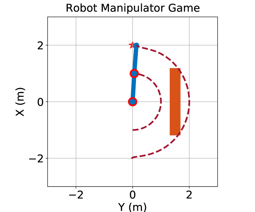
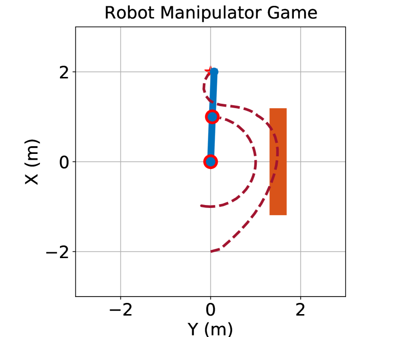
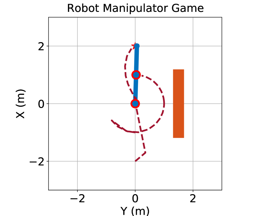
We have conducted extensive experiments to test the proposed method, including various numerical examples, a user study on two human-robot games, and a real-world quadrotor experiment. The results show that the proposed method is significantly more effective (higher success rate), efficient/effortless (less human corrections needed), and potentially more accessible (fewer early wasted trials) than the state-of-the-art robot learning frameworks.

I-A Related Work

I-A1 One-time Learning from Demonstrations

To learn an objective function from demonstrations, routine methods are inverse optimal control [12, 13, 14] or inverse reinforcement learning [15, 16, 17], where an objective function is learned from optimal demonstrations and subsequently used for control or planning. Successful LfD applications include autonomous driving [2], robot manipulation [3], and motion planning [4]. Despite the notable success [18, 19, 20], LfD could be inconvenient in practice. First, demonstrations in LfD are usually collected in a one-time manner and the robot learning is offline. In the case where demonstration data is insufficient to recover an objective function, such as low data informativeness as discussed in [5], or significantly deviating from the optima, the data has to be re-collected and the training has to be re-run. Second, existing LfD [13, 14, 15, 16, 17] normally requires the optimality of demonstrations, which are challenging to collect for robots with high degree-of-freedoms. For example, when providing demonstrations for a humanoid robot, a user has to account for the robot’s motion of all degrees of freedom in a spatially and temporally consistent manner [6].

I-A2 Incrementally Learning from Corrections/feedback

Compared to one-time LfD, learning from corrections or feedback enables a user to incrementally improve robot motion, making it more suitable for non-expert users who cannot provide optimal demonstrations in a one-time fashion [10]. The key assumption is that robot motion after correction achieves a higher reward (or a lower cost) than before correction. Under this assumption, [6] develops a co-active learning method to update the robot objective function using user feedback. The user feedback includes a human either selecting the top-ranked robot trajectory among all candidates or physically demonstrating a preferred trajectory to the robot. By defining a regret, which quantifies the average misalignment between the value of robot motion and that of the desired motion under the true objective function, [6] shows the convergence of the regret. But since regret only considers values of an objective function, it cannot directly tell and guarantee that the learned objective function itself is converging towards the true one. As we will show in Section V-C, the objective function can converge to a local solution instead of a true one.

Recently, [7, 8, 9] handle learning from corrections through the perspective of the partially observable Markov decision process (POMDP). Here, human corrections are viewed as observations about the unknown objective function parameter. By approximating the observation model and applying the maximum a posteriori estimation, they obtain a learning formula similar to the co-active learning [6]. Along with this perspective, some variants have been recently developed to particularly account for the uncertainties of human corrections. For example, [21] simultaneously estimates a rationality coefficient to characterize the rationality confidence of human corrections. [9] fits the inverse reinforcement learning into a Kalman filter framework to quantitatively capture the uncertainty of the estimation.

Both the above co-active learning and POMDP-based learning require a human to carefully choose the magnitude correction that improves robot motion. As we will detail in Section II, choosing a valid magnitude correction is difficult, especially when a robot gets closer to the desired motion, because the allowable magnitude of a correction has to lie in a shrinking level set. Near the desired motion, a human could easily over-correct the robot, i.e., applying too large corrections that adversely drive the robot away from the desired motion, making the algorithm diverge or even fail. We will experimentally show this difficulty in Section V-C. Moreover, due to the sparsity of human corrections, all the above methods require a dedicated step to obtain a human ‘intended’ trajectory for each correction. In the co-active learning, a robot needs to switch to a screening mode to obtain a human preferred trajectory, and in the POMDP-based method, a human intended trajectory is created by trajectory deformation [22]. These pre-processing steps may not only introduce more hyperparameters but also add some artifacts that could undermine the learning performance [8]

Very recently, [23] directly learns a desired trajectory from human physical interactions, then a robot tracks the learned trajectory using linear–quadratic regulator (LQR) controllers. They minimize a trajectory distance loss, and the learning update is based on the assumption that the direction of a human correction is exactly aligned with the deepest gradient descent of the distance loss. While that work is related to our work in the sense that they both use the direction of a human correction, our work, however, focuses on learning an objective function instead of learning the desired trajectory directly. Importantly, we do not restrict the direction of a correction to be exactly aligned with the deepest gradient descent, but any correction as long as it has a direction that decreases the cost of robot motion. The above two distinctions lead to a new method of our work, which has a strong theoretical guarantee for learning convergence.

Finally, we want to mention that most of the existing methods [7, 8, 9, 23] lack theoretical guarantee about the learning performance. The only work that attempts to do so is [6], where a regret bound is shown. As discussed previously, such regret is an indicator of the misalignment of the values of the objective function, and cannot directly tell or guarantee the convergence of the objective function itself. In this paper, we will directly characterize the convergence of the learned objective function towards the true function that is induced by human corrections.

I-B Contributions

To give readers a high-level picture of the proposed method, we show an overview in Fig. 2. We claim the following contributions of the proposed method.

Refer to caption
Figure 2: An overview of the proposed algorithm.
  • (I)

    The proposed method learns an objective function from human directional corrections. It only requires that a correction, regardless of its magnitude, points in a direction of improving robot motion. As we will show in Sections II and V-C, the allowable corrections that satisfy this requirement always account for half of the input space, making it more flexible for users to choose corrections from. Also, unlike existing methods, the proposed method directly learns from sparse directional corrections without a pre-processing step of creating an ‘intended’ trajectory.

  • (II)

    The proposed learning algorithm has strong theoretical foundations. First, the proposed learning method is based on the cutting plane technique, which has straightforward geometric interpretations, as shown in Fig. 2. Second, we have established the theoretical results to show the convergence of the method towards finding the true objective function induced by all corrections.

Numerical examples, a user study on two human-robot games, and a real-world quadrotor experiment confirm the efficacy and convergence of the proposed algorithm. The user study and real-world experiment further show that the proposed method is significantly more effective (higher success rate), efficient/effortless (fewer corrections needed), and potentially more accessible (fewer early wasted trials) than the state-of-the-art methods.

In what follows, Section II describes the problem formulation. Section III outlines the main algorithm and presents its geometric interpretation. Section IV provides the theoretical results of the algorithm and its detailed implementation. Various numerical examples and comparisons are given in Section V. Section VI presents a user study and Section VII provides a real-world experiment. Conclusions are drawn in Section VIII. The appendix includes the proof, discussion, and possible extension of this work.

II Problem Formulation

Consider a robot with the following dynamics and the initial condition:

𝒙t+1=𝒇(𝒙t,𝒖t),with𝒙0,subscript𝒙𝑡1𝒇subscript𝒙𝑡subscript𝒖𝑡withsubscript𝒙0\boldsymbol{x}_{t+1}=\boldsymbol{f}(\boldsymbol{x}_{t},\boldsymbol{u}_{t}),\quad\text{with}\quad\boldsymbol{x}_{0}, (1)

where 𝒙tnsubscript𝒙𝑡superscript𝑛\boldsymbol{x}_{t}\in\mathbb{R}^{n} is the robot state, 𝒖tmsubscript𝒖𝑡superscript𝑚\boldsymbol{u}_{t}\in\mathbb{R}^{m} is the control input, 𝒇:n×mn:𝒇maps-tosuperscript𝑛superscript𝑚superscript𝑛\boldsymbol{f}:\mathbb{R}^{n}\times\mathbb{R}^{m}\mapsto\mathbb{R}^{n} is differentiable, and t=1,2,𝑡12t=1,2,\cdots is the time step. As commonly used in objective learning methods [15, 16, 17, 10, 6, 7, 8, 9, 5, 14], suppose that the robot cost function has the following parameterized form:

J(𝒖0:T,𝜽)=t=0T𝜽𝖳ϕ(𝒙t,𝒖t)+h(𝒙T+1),𝐽subscript𝒖:0𝑇𝜽superscriptsubscript𝑡0𝑇superscript𝜽𝖳bold-italic-ϕsubscript𝒙𝑡subscript𝒖𝑡subscript𝒙𝑇1J(\boldsymbol{u}_{0:T},\boldsymbol{\theta})=\sum\nolimits_{t=0}^{T}\boldsymbol{\theta}^{\mkern-1.5mu\mathsf{T}}\boldsymbol{\phi}(\boldsymbol{x}_{t},\boldsymbol{u}_{t})+h(\boldsymbol{x}_{T+1}), (2)

where ϕ:n×mr:bold-italic-ϕmaps-tosuperscript𝑛superscript𝑚superscript𝑟\boldsymbol{\phi}:\mathbb{R}^{n}\times\mathbb{R}^{m}\mapsto\mathbb{R}^{r} is a vector of the pre-defined features (basis functions); 𝜽r𝜽superscript𝑟\boldsymbol{\theta}\in\mathbb{R}^{r} is a vector of weights, which are tunable; and h(𝒙T+1)subscript𝒙𝑇1h(\boldsymbol{x}_{T+1}) is the final cost on the robot final state 𝒙T+1subscript𝒙𝑇1\boldsymbol{x}_{T+1}, such as penalizing the distance between 𝒙T+1subscript𝒙𝑇1\boldsymbol{x}_{T+1} and a given goal state 𝒙goalsuperscript𝒙goal\boldsymbol{x}^{\text{goal}}, h(𝒙T+1)=𝒙goal𝒙T+12subscript𝒙𝑇1superscriptdelimited-∥∥superscript𝒙goalsubscript𝒙𝑇12{h}(\boldsymbol{x}_{T+1})=\lVert\boldsymbol{x}^{\text{goal}}-\boldsymbol{x}_{T+1}\rVert^{2}. Note that depending on specific applications, the final cost term h(𝒙T+1)subscript𝒙𝑇1{h}(\boldsymbol{x}_{T+1}) can be either absent, i.e., h(𝒙T+1)=0subscript𝒙𝑇10{h}(\boldsymbol{x}_{T+1})=0, or also parameterized in a weighted-feature form with the weights to be learned jointly with 𝜽𝜽\boldsymbol{\theta}. The method developed in this paper can sufficiently handle either cases with little modifications. For a fixed choice of 𝜽𝜽\boldsymbol{\theta}, the robot plans a sequence of inputs 𝒖0:Tsubscript𝒖:0𝑇\boldsymbol{u}_{0:T} over time horizon T𝑇T by (locally) optimizing the cost function (2) subject to (1), producing a trajectory

𝝃𝜽={𝒙0:T+1𝜽,𝒖0:T𝜽}.subscript𝝃𝜽superscriptsubscript𝒙:0𝑇+1𝜽superscriptsubscript𝒖:0𝑇𝜽\boldsymbol{\xi}_{\boldsymbol{\theta}}=\left\{\boldsymbol{x}_{0:T\text{+}1}^{\boldsymbol{\theta}},\boldsymbol{u}_{0:T}^{\boldsymbol{\theta}}\right\}. (3)

In the following text, we occasionally write the cost function (2) as J(𝜽)𝐽𝜽J(\boldsymbol{\theta}) for ease of readability.

For a specific task, suppose that a human user expects the robot to minimize an implicit cost function J(𝜽)𝐽superscript𝜽J(\boldsymbol{\theta}^{*}) in the same form of (2) but with unknown 𝜽superscript𝜽\boldsymbol{\theta}^{*}. We call 𝜽superscript𝜽\boldsymbol{\theta}^{*} the true weight vector. In general, a human user may neither explicitly write down the value of 𝜽superscript𝜽\boldsymbol{\theta}^{*} nor demonstrate the corresponding desired trajectory 𝝃𝜽subscript𝝃superscript𝜽\boldsymbol{\xi}_{\boldsymbol{\theta}^{*}}, but the human user can tell whether the robot motion trajectory is desired or not. A robot trajectory is desired if it minimizes the implicit J(𝜽)𝐽superscript𝜽J(\boldsymbol{\theta}^{*}); otherwise, it is not desired. In order for the robot to learn J(𝜽)𝐽superscript𝜽J(\boldsymbol{\theta}^{*}) (and thus generate the desired trajectory 𝝃𝜽subscript𝝃superscript𝜽\boldsymbol{\xi}_{\boldsymbol{\theta}^{*}}), the human user is only able to make corrections to the robot motion. After receiving each human correction, the robot updates its guess 𝜽𝜽\boldsymbol{\theta} towards the true 𝜽superscript𝜽\boldsymbol{\theta}^{*}. This procedure has been shown in Fig. 1.

Specifically, the process of a robot learning from human directional corrections is iterative, as shown in Fig. 2. Each iteration basically includes three steps: robot planning (& execution), human correction, and robot update. Let k=1,2,3,𝑘123k=1,2,3,\cdots, be the iteration index and let 𝜽ksubscript𝜽𝑘\boldsymbol{\theta}_{k} denote the robot’s guess of the weight vector at iteration k𝑘k. At k=1𝑘1k=1, the robot is initialized with an arbitrary guess 𝜽1subscript𝜽1\boldsymbol{\theta}_{1}. At iteration k𝑘k, the robot first performs motion planning, i.e. solving 𝝃𝜽ksubscript𝝃subscript𝜽𝑘\boldsymbol{\xi}_{\boldsymbol{\theta}_{k}} by minimizing the cost function J(𝜽k)𝐽subscript𝜽𝑘J(\boldsymbol{\theta}_{k}) in (2) subject to its dynamics in (1). During the robot executing 𝝃𝜽ksubscript𝝃subscript𝜽𝑘\boldsymbol{\xi}_{\boldsymbol{\theta}_{k}}, the human user observes 𝝃𝜽ksubscript𝝃subscript𝜽𝑘\boldsymbol{\xi}_{\boldsymbol{\theta}_{k}} and applies a correction, denoted by 𝒂tkmsubscript𝒂subscript𝑡𝑘superscript𝑚\boldsymbol{a}_{t_{k}}\in\mathbb{R}^{m}, to the robot in its input space. Here, tk{0,1,,T}subscript𝑡𝑘01𝑇{t_{k}}\in\{0,1,\cdots,T\} is called correction time, indicating at which time step the correction 𝒂tksubscript𝒂subscript𝑡𝑘\boldsymbol{a}_{t_{k}} is made. After receiving 𝒂tksubscript𝒂subscript𝑡𝑘\boldsymbol{a}_{t_{k}}, the robot updates its guess 𝜽ksubscript𝜽𝑘\boldsymbol{\theta}_{k} to 𝜽k+1subscript𝜽𝑘1\boldsymbol{\theta}_{k+1} based on an update rule developed later.

One distinguishing feature of our method is that we assume that each human correction 𝒂tksubscript𝒂subscript𝑡𝑘\boldsymbol{a}_{t_{k}} satisfies

J(𝒖0:T𝜽k,𝜽),𝒂k>0,k=1,2,3,.formulae-sequence𝐽superscriptsubscript𝒖:0𝑇subscript𝜽𝑘superscript𝜽subscript𝒂𝑘0𝑘123\left\langle-\nabla J(\boldsymbol{u}_{0:T}^{\boldsymbol{\theta}_{k}},\boldsymbol{\theta}^{*}),\,\,\boldsymbol{{a}}_{k}\right\rangle>0,\quad k=1,2,3,\cdots. (4)

Here,

𝒂k=[𝟎𝖳,𝒂tk𝖳,,𝟎𝖳]𝖳m(T+1),subscript𝒂𝑘superscriptmatrixsuperscript0𝖳superscriptsubscript𝒂subscript𝑡𝑘𝖳superscript0𝖳𝖳superscript𝑚𝑇1\boldsymbol{{a}}_{k}=\begin{bmatrix}\boldsymbol{0}^{\mkern-1.5mu\mathsf{T}}&\cdots,&\boldsymbol{a}_{t_{k}}^{\mkern-1.5mu\mathsf{T}},&\cdots,\boldsymbol{0}^{\mkern-1.5mu\mathsf{T}}\end{bmatrix}^{\mkern-1.5mu\mathsf{T}}\in\mathbb{R}^{m{(T+1)}}, (5)

with 𝒂tksubscript𝒂subscript𝑡𝑘\boldsymbol{a}_{t_{k}} filled at the tksubscript𝑡𝑘t_{k}th entry and 𝟎m0superscript𝑚\boldsymbol{0}\in\mathbb{R}^{m} elsewhere. Here, ,\left\langle\cdot,\cdot\right\rangle is the dot product, and J(𝒖0:T𝜽k,𝜽)𝐽superscriptsubscript𝒖:0𝑇subscript𝜽𝑘superscript𝜽-\nabla J(\boldsymbol{u}_{0:T}^{\boldsymbol{\theta}_{k}},\boldsymbol{\theta}^{*}) is the gradient-descent of J(𝜽)𝐽superscript𝜽J(\boldsymbol{\theta}^{*}) with respect to 𝒖0:Tsubscript𝒖:0𝑇\boldsymbol{u}_{0:T} evaluated at the robot current trajectory 𝝃𝜽k={𝒙0:T+1𝜽k,𝒖0:T𝜽k}subscript𝝃subscript𝜽𝑘superscriptsubscript𝒙:0𝑇+1subscript𝜽𝑘superscriptsubscript𝒖:0𝑇subscript𝜽𝑘\boldsymbol{\xi}_{\boldsymbol{\theta}_{k}}=\{\boldsymbol{x}_{0:T\text{+}1}^{\boldsymbol{\theta}_{k}},\boldsymbol{u}_{0:T}^{\boldsymbol{\theta}_{k}}\}. Note that (4) does not require a specific value to the magnitude of 𝒂tksubscript𝒂subscript𝑡𝑘\boldsymbol{a}_{t_{k}} but requires its direction roughly around the gradient-descent direction of J(𝜽)𝐽superscript𝜽J(\boldsymbol{\theta}^{*}). It means that the correction 𝒂ksubscript𝒂𝑘\boldsymbol{{a}}_{k} aims to guide the robot motion 𝝃𝜽ksubscript𝝃subscript𝜽𝑘\boldsymbol{\xi}_{\boldsymbol{\theta}_{k}} towards a lower cost under J(𝜽)𝐽superscript𝜽J(\boldsymbol{\theta}^{*}) unless the trajectory is desired. Thus, we call 𝒂tksubscript𝒂subscript𝑡𝑘\boldsymbol{a}_{t_{k}} a directional correction.

In practice, one always needs to account for human’s noisy or imperfect corrections. Thus, we modify (4) as follows

𝔼𝒂kJ(𝒖0:T𝜽k,𝜽),𝒂ksubscript𝔼subscript𝒂𝑘𝐽superscriptsubscript𝒖:0𝑇subscript𝜽𝑘superscript𝜽subscript𝒂𝑘\displaystyle\operatorname{\mathbb{E}}_{\boldsymbol{a}_{k}}\left\langle-\nabla J(\boldsymbol{u}_{0:T}^{\boldsymbol{\theta}_{k}},\boldsymbol{\theta}^{*}),\,\,\boldsymbol{{a}}_{k}\right\rangle (6a)
=\displaystyle= J(𝒖0:T𝜽k,𝜽),𝔼𝒂k(𝒂k)𝐽superscriptsubscript𝒖:0𝑇subscript𝜽𝑘superscript𝜽subscript𝔼subscript𝒂𝑘subscript𝒂𝑘\displaystyle\left\langle-\nabla J(\boldsymbol{u}_{0:T}^{\boldsymbol{\theta}_{k}},\boldsymbol{\theta}^{*}),\,\,\operatorname{\mathbb{E}}_{\boldsymbol{a}_{k}}(\boldsymbol{{a}}_{k})\right\rangle
=\displaystyle= J(𝒖0:T𝜽k,𝜽),𝒂¯k>0,k=1,2,,formulae-sequence𝐽superscriptsubscript𝒖:0𝑇subscript𝜽𝑘superscript𝜽subscriptbold-¯𝒂𝑘0𝑘12\displaystyle\left\langle-\nabla J(\boldsymbol{u}_{0:T}^{\boldsymbol{\theta}_{k}},\boldsymbol{\theta}^{*}),\,\,\boldsymbol{\bar{a}}_{k}\right\rangle>0,\quad k=1,2,...,
where
𝒂¯k=𝔼𝒂k(𝒂k).subscriptbold-¯𝒂𝑘subscript𝔼subscript𝒂𝑘subscript𝒂𝑘\boldsymbol{\bar{a}}_{k}=\operatorname{\mathbb{E}}_{\boldsymbol{a}_{k}}(\boldsymbol{{a}}_{k}). (6b)

Here, 𝔼()𝔼\operatorname{\mathbb{E}}(\cdot) is the expectation with respect to the human correction data 𝒂ksubscript𝒂𝑘\boldsymbol{a}_{k}. (6) says that the original assumption (4) can be met in expectation; in other words, the robot can receive and average human’s multiple directional corrections before one update of the cost function is made. There are two ways to implement multiple corrections. The most convenient way is that a human user applies multiple directional corrections at different time steps but all within the same execution of the robot motion 𝝃𝜽ksubscript𝝃subscript𝜽𝑘\boldsymbol{\xi}_{\boldsymbol{\theta}_{k}}, i.e., the robot executes the current plan 𝝃𝜽ksubscript𝝃subscript𝜽𝑘\boldsymbol{\xi}_{\boldsymbol{\theta}_{k}} just once. The second way is that the multiple corrections are applied in the multiple repetitions of the execution of 𝝃𝜽ksubscript𝝃subscript𝜽𝑘\boldsymbol{\xi}_{\boldsymbol{\theta}_{k}}, i.e., the robot executes the same plan 𝝃𝜽ksubscript𝝃subscript𝜽𝑘\boldsymbol{\xi}_{\boldsymbol{\theta}_{k}} for multiple times. Whichever implementation, by taking the expectation of human’s multiple directional corrections 𝒂¯k=𝔼𝒂k(𝒂k)subscriptbold-¯𝒂𝑘subscript𝔼subscript𝒂𝑘subscript𝒂𝑘\boldsymbol{\bar{a}}_{k}=\operatorname{\mathbb{E}}_{\boldsymbol{a}_{k}}(\boldsymbol{{a}}_{k}), (6) permits noisy and imperfect human directional corrections. The similar strategies have also been adopted in [6].

The problem of interest in this paper is that given human (averaged) directional corrections 𝒂¯ksubscriptbold-¯𝒂𝑘\boldsymbol{\bar{a}}_{k} satisfying the assumption (6), we aim to develop a rule to update the robot weight vector guess 𝜽ksubscript𝜽𝑘\boldsymbol{\theta}_{k} such that 𝜽ksubscript𝜽𝑘\boldsymbol{\theta}_{k} converges to 𝜽superscript𝜽\boldsymbol{\theta}^{*} as k=1,2,3,𝑘123k=1,2,3,....

Remark 1.

We assume that human corrections 𝐚tkmsubscript𝐚subscript𝑡𝑘superscript𝑚\boldsymbol{a}_{t_{k}}\in\mathbb{R}^{m} are in the robot input space, which means that 𝐚tksubscript𝐚subscript𝑡𝑘\boldsymbol{a}_{t_{k}} can be directly added to robot input 𝐮tksubscript𝐮subscript𝑡𝑘\boldsymbol{u}_{t_{k}}. This can be readily fulfilled in some applications such as autonomous vehicles, where a user directly changes the steering angle of a vehicle. For other cases where the corrections are not readily in the robot input space, it could be met via some specific interfaces (or computation), which map correction signals to the robot input space. For example, when a human interacts with the end effector of a robot manipulator, one can convert the task-space contact force to the joint torques via Jacobian. Then, 𝐚tksubscript𝐚subscript𝑡𝑘\boldsymbol{a}_{t_{k}} is the mapped correction. The reason why we do not consider the corrections in the state space is that 1) corrections in input spaces may be easier to implement, as shown in our later experiments, and 2) corrections in state spaces can be infeasible for the under-actuated robot systems [24].
Refer to caption
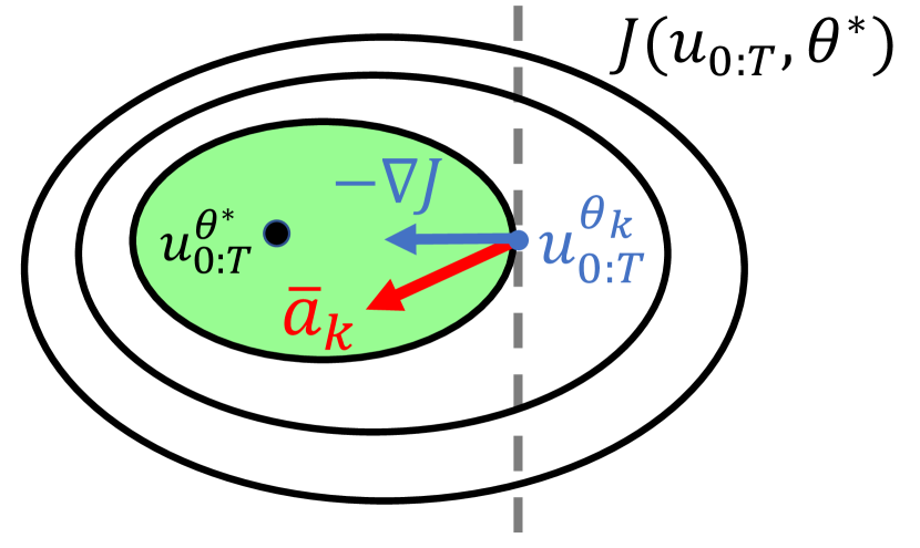
(a) Allowable region (green) of magnitude corrections.
Refer to caption
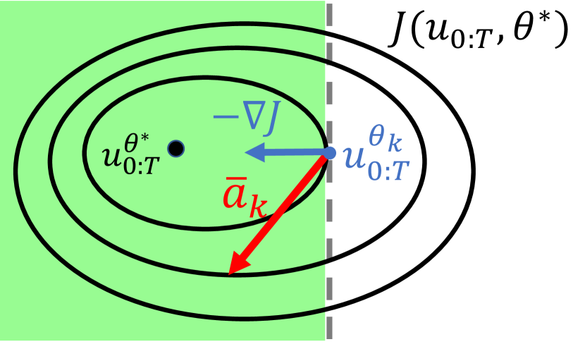
(b) Allowable region (green) of directional corrections.
Figure 3: Magnitude corrections v.s. directional corrections. Contours (circles) and the desired trajectory 𝒖0:T𝜽superscriptsubscript𝒖:0𝑇superscript𝜽\boldsymbol{u}_{0:T}^{\boldsymbol{\theta}^{*}} (black dot) of the true cost function J(𝜽)𝐽superscript𝜽J(\boldsymbol{\theta}^{*}) are plotted. (a) Green region (a sub-level set) indicates all allowable magnitude corrections 𝒂¯ksubscriptbold-¯𝒂𝑘\boldsymbol{\bar{a}}_{k} that satisfy J(𝒖0:T𝜽k+𝒂¯k,𝜽)<J(𝒖0:T𝜽k,𝜽)𝐽superscriptsubscript𝒖:0𝑇subscript𝜽𝑘subscriptbold-¯𝒂𝑘superscript𝜽𝐽superscriptsubscript𝒖:0𝑇subscript𝜽𝑘superscript𝜽J(\boldsymbol{u}_{0:T}^{\boldsymbol{{\theta}}_{k}}+\boldsymbol{\bar{a}}_{k},\boldsymbol{\theta}^{*}){<}J(\boldsymbol{u}_{0:T}^{\boldsymbol{{\theta}}_{k}},\boldsymbol{\theta}^{*}). (b) Green region (half of the input space) indicates all allowable directional corrections 𝒂¯ksubscriptbold-¯𝒂𝑘\boldsymbol{\bar{a}}_{k} that satisfy J(𝒖0:T𝜽k,𝜽),𝒂¯k>0𝐽superscriptsubscript𝒖:0𝑇subscript𝜽𝑘superscript𝜽subscriptbold-¯𝒂𝑘0\langle-\nabla J(\boldsymbol{u}_{0:T}^{\boldsymbol{\theta}_{k}},\boldsymbol{\theta}^{*}),\boldsymbol{\bar{a}}_{k}\rangle{>}0.
Remark 2.

Assumption (4) on directional correction 𝐚tksubscript𝐚subscript𝑡𝑘\boldsymbol{a}_{{t}_{k}} is less restrictive than ones in [7, 8, 9, 6] using magnitude corrections, which assume the cost of the corrected robot trajectory 𝐮0:T𝛉k+𝐚¯ksuperscriptsubscript𝐮:0𝑇subscript𝛉𝑘subscriptbold-¯𝐚𝑘\boldsymbol{u}_{0:T}^{\boldsymbol{{\theta}}_{k}}+\boldsymbol{\bar{a}}_{k} is lower than that of the robot original motion 𝐮0:T𝛉ksuperscriptsubscript𝐮:0𝑇subscript𝛉𝑘\boldsymbol{u}_{0:T}^{\boldsymbol{\theta}_{k}}, i.e., J(𝐮0:T𝛉k+𝐚¯k,𝛉)<J(𝐮0:T𝛉k,𝛉)𝐽superscriptsubscript𝐮:0𝑇subscript𝛉𝑘subscriptbold-¯𝐚𝑘superscript𝛉𝐽superscriptsubscript𝐮:0𝑇subscript𝛉𝑘superscript𝛉\small J(\boldsymbol{u}_{0:T}^{\boldsymbol{{\theta}}_{k}}+\boldsymbol{\bar{a}}_{k},\boldsymbol{\theta}^{*}){<}J(\boldsymbol{u}_{0:T}^{\boldsymbol{{\theta}}_{k}},\boldsymbol{\theta}^{*}). As shown in Fig. 3, their assumptions usually lead to the restriction of correction magnitude. Specifically, to satisfy J(𝐮0:T𝛉k+𝐚¯k,𝛉)<J(𝐮0:T𝛉k,𝛉)𝐽superscriptsubscript𝐮:0𝑇subscript𝛉𝑘subscriptbold-¯𝐚𝑘superscript𝛉𝐽superscriptsubscript𝐮:0𝑇subscript𝛉𝑘superscript𝛉\small J(\boldsymbol{u}_{0:T}^{\boldsymbol{{\theta}}_{k}}+\boldsymbol{\bar{a}}_{k},\boldsymbol{\theta}^{*}){<}J(\boldsymbol{u}_{0:T}^{\boldsymbol{{\theta}}_{k}},\boldsymbol{\theta}^{*}), 𝐚¯kdelimited-∥∥subscriptbold-¯𝐚𝑘\lVert\boldsymbol{\bar{a}}_{k}\rVert has to be chosen from the J(𝐮0:T𝛉k,𝛉)𝐽superscriptsubscript𝐮:0𝑇subscript𝛉𝑘superscript𝛉\small J(\boldsymbol{u}_{0:T}^{\boldsymbol{{\theta}}_{k}},\boldsymbol{\theta}^{*})-sublevel set of J(𝛉)𝐽superscript𝛉J(\boldsymbol{\theta}^{*}), as shown by the green region in Fig. 3(a). Furthermore, this region will shrink as 𝐮0:T𝛉ksuperscriptsubscript𝐮:0𝑇subscript𝛉𝑘\boldsymbol{u}_{0:T}^{\boldsymbol{{\theta}}_{k}} gets close to the desired trajectory 𝐮0:T𝛉superscriptsubscript𝐮:0𝑇superscript𝛉\boldsymbol{u}_{0:T}^{\boldsymbol{\theta}^{*}} (black dot), thus making 𝐚¯kdelimited-∥∥subscriptbold-¯𝐚𝑘\lVert\boldsymbol{\bar{a}}_{k}\rVert more difficult to choose. In contrast, the directional corrections satisfying (4) always account for half of the input space, as shown by the green region in Fig. 3(b). A human user can choose any correction as long as its direction lies in the half space of the gradient descent of J(𝛉)𝐽superscript𝛉J(\boldsymbol{\theta}^{*}). Thus, (4) would be more likely to be satisfied for non-expert users. We will experimentally show this advantage later in Section V-C and Section VI.

III Main Algorithm Outline and its Geometric Interpretation

In this section, we will outline the proposed main algorithm and present its geometric interpretation.

III-A Hyperplane for Each Directional Correction

Before developing the main algorithm, we first show that the condition (6) equals a linear inequality imposed on the true 𝜽superscript𝜽\boldsymbol{\theta}^{*}. This has been formally stated by the following lemma.

Lemma 1.

Suppose that the current guess of the weight vector is 𝛉ksubscript𝛉𝑘\boldsymbol{\theta}_{k}, and the robot trajectory 𝛏𝛉k={𝐱0:T+1𝛉k,𝐮0:T𝛉k}subscript𝛏subscript𝛉𝑘superscriptsubscript𝐱:0𝑇+1subscript𝛉𝑘superscriptsubscript𝐮:0𝑇subscript𝛉𝑘\boldsymbol{\xi}_{\boldsymbol{\theta}_{k}}{=}\{\boldsymbol{x}_{0:T\text{+}1}^{\boldsymbol{\theta}_{k}},\boldsymbol{u}_{0:T}^{\boldsymbol{\theta}_{k}}\} is a result of (locally) minimizing J(𝛉k)𝐽subscript𝛉𝑘J(\boldsymbol{\theta}_{k}) in (2) subject to dynamics (1). For 𝛏𝛉ksubscript𝛏subscript𝛉𝑘\boldsymbol{\xi}_{\boldsymbol{\theta}_{k}}, given a human (averaged) directional correction 𝐚¯tksubscriptbold-¯𝐚subscript𝑡𝑘\boldsymbol{\bar{a}}_{t_{k}} satisfying (6), one has

𝒉k,𝜽+bk<0,k=1,2,3,formulae-sequencesubscript𝒉𝑘superscript𝜽subscript𝑏𝑘0𝑘123\left\langle\boldsymbol{h}_{k},\boldsymbol{\theta}^{*}\right\rangle+b_{k}<0,\quad k=1,2,3\cdots, (7)

with

𝒉ksubscript𝒉𝑘\displaystyle\boldsymbol{h}_{k} =𝑯1𝖳(𝒙0:T+1𝜽k,𝒖0:T𝜽k)𝒂¯kr,absentsuperscriptsubscript𝑯1𝖳superscriptsubscript𝒙:0𝑇+1subscript𝜽𝑘superscriptsubscript𝒖:0𝑇subscript𝜽𝑘subscriptbold-¯𝒂𝑘superscript𝑟\displaystyle=\boldsymbol{H}_{1}^{\mkern-1.5mu\mathsf{T}}(\boldsymbol{x}_{0:{T\text{+}1}}^{\boldsymbol{\theta}_{k}},\boldsymbol{u}_{0:T}^{\boldsymbol{\theta}_{k}})\boldsymbol{\bar{a}}_{k}\,\,\in\mathbb{R}^{r}, (8a)
bksubscript𝑏𝑘\displaystyle b_{k} =𝒂¯k𝖳𝑯2(𝒙0:T+1𝜽k,𝒖0:T𝜽k)h(𝒙T+1𝜽k).absentsuperscriptsubscriptbold-¯𝒂𝑘𝖳subscript𝑯2superscriptsubscript𝒙:0𝑇+1subscript𝜽𝑘superscriptsubscript𝒖:0𝑇subscript𝜽𝑘superscriptsubscript𝒙𝑇1subscript𝜽𝑘\displaystyle=\boldsymbol{\bar{a}}_{k}^{\mkern-1.5mu\mathsf{T}}\boldsymbol{H}_{2}(\boldsymbol{x}_{0:{T\text{+}1}}^{\boldsymbol{\theta}_{k}},\boldsymbol{u}_{0:T}^{\boldsymbol{\theta}_{k}})\nabla h(\boldsymbol{x}_{T+1}^{\boldsymbol{\theta}_{k}})\,\,\in\mathbb{R}. (8b)

Here, 𝐚¯ksubscriptbold-¯𝐚𝑘\boldsymbol{\bar{a}}_{k} is defined in (6b); h(𝐱T+1𝛉k)superscriptsubscript𝐱𝑇1subscript𝛉𝑘\nabla h(\boldsymbol{x}_{T+1}^{\boldsymbol{\theta}_{k}}) is the gradient of the final cost h(𝐱T+1)subscript𝐱𝑇1h(\boldsymbol{x}_{T+1}) in (2) evaluated at 𝐱T+1𝛉ksuperscriptsubscript𝐱𝑇1subscript𝛉𝑘\boldsymbol{x}_{T+1}^{\boldsymbol{\theta}_{k}}; 𝐇1(𝐱0:T+1𝛉k,𝐮0:T𝛉k)subscript𝐇1subscriptsuperscript𝐱subscript𝛉𝑘:0𝑇+1subscriptsuperscript𝐮subscript𝛉𝑘:0𝑇\boldsymbol{H}_{1}(\boldsymbol{x}^{\boldsymbol{\theta}_{k}}_{0:T\text{+}1},\boldsymbol{u}^{\boldsymbol{\theta}_{k}}_{0:T}) and 𝐇2(𝐱0:T+1𝛉k,𝐮0:T𝛉k)subscript𝐇2subscriptsuperscript𝐱subscript𝛉𝑘:0𝑇+1subscriptsuperscript𝐮subscript𝛉𝑘:0𝑇\boldsymbol{H}_{2}(\boldsymbol{x}^{\boldsymbol{\theta}_{k}}_{0:T\text{+}1},\boldsymbol{u}^{\boldsymbol{\theta}_{k}}_{0:T}) are computed as:

𝑯1(𝒙0:T+1𝜽k,𝒖0:T𝜽k)subscript𝑯1subscriptsuperscript𝒙subscript𝜽𝑘:0𝑇+1subscriptsuperscript𝒖subscript𝜽𝑘:0𝑇\displaystyle\boldsymbol{H}_{1}(\boldsymbol{x}^{\boldsymbol{\theta}_{k}}_{0:T\text{+}1},\boldsymbol{u}^{\boldsymbol{\theta}_{k}}_{0:T}) =[𝑭u𝑭x1𝚽x+𝚽uϕ𝖳𝒖T𝜽k]m(T+1)×r,absentmatrixsubscript𝑭𝑢superscriptsubscript𝑭𝑥1subscript𝚽𝑥subscript𝚽𝑢superscriptbold-italic-ϕ𝖳subscriptsuperscript𝒖subscript𝜽𝑘𝑇superscript𝑚𝑇+1𝑟\displaystyle{=}\begin{bmatrix}\boldsymbol{F}_{u}\boldsymbol{F}_{x}^{{-}1}\boldsymbol{\Phi}_{x}{+}\boldsymbol{\Phi}_{u}\\ \frac{\partial\boldsymbol{\phi}^{\mkern-1.5mu\mathsf{T}}}{\partial\boldsymbol{u}^{\boldsymbol{\theta}_{k}}_{T}}\\ \end{bmatrix}\in\mathbb{R}^{m(T\text{+}1)\times r}, (9a)
𝑯2(𝒙0:T+1𝜽k,𝒖0:T𝜽k)subscript𝑯2subscriptsuperscript𝒙subscript𝜽𝑘:0𝑇+1subscriptsuperscript𝒖subscript𝜽𝑘:0𝑇\displaystyle\boldsymbol{H}_{2}(\boldsymbol{x}^{\boldsymbol{\theta}_{k}}_{0:T\text{+}1},\boldsymbol{u}^{\boldsymbol{\theta}_{k}}_{0:T}) =[𝑭u𝑭x1𝑽𝒇𝖳𝒖T𝜽k]m(T+1)×n,absentmatrixsubscript𝑭𝑢superscriptsubscript𝑭𝑥1𝑽superscript𝒇𝖳subscriptsuperscript𝒖subscript𝜽𝑘𝑇superscript𝑚𝑇+1𝑛\displaystyle{=}\begin{bmatrix}\boldsymbol{F}_{u}\boldsymbol{F}_{x}^{-1}\boldsymbol{V}\\ \frac{\partial\boldsymbol{f}^{\mkern-1.5mu\mathsf{T}}}{\partial\boldsymbol{u}^{\boldsymbol{\theta}_{k}}_{T}}\end{bmatrix}\in\mathbb{R}^{m(T\text{+}1)\times n}, (9b)

with

𝑭xsubscript𝑭𝑥\displaystyle\boldsymbol{F}_{x} =[I𝒇𝖳𝒙1𝜽k𝟎𝟎𝟎I𝟎𝟎𝟎𝟎I𝒇𝖳𝒙T-1𝜽k𝟎𝟎I],𝚽x=[ϕ𝖳𝒙1𝜽kϕ𝖳𝒙2𝜽kϕ𝖳𝒙T𝜽k],formulae-sequenceabsentmatrix𝐼superscript𝒇𝖳subscriptsuperscript𝒙subscript𝜽𝑘1000𝐼0000𝐼superscript𝒇𝖳subscriptsuperscript𝒙subscript𝜽𝑘𝑇-100missing-subexpression𝐼subscript𝚽𝑥matrixsuperscriptbold-italic-ϕ𝖳subscriptsuperscript𝒙subscript𝜽𝑘1superscriptbold-italic-ϕ𝖳subscriptsuperscript𝒙subscript𝜽𝑘2superscriptbold-italic-ϕ𝖳subscriptsuperscript𝒙subscript𝜽𝑘𝑇\displaystyle{=}\begin{bmatrix}{I}&\frac{-\partial\boldsymbol{f}^{\mkern-1.5mu\mathsf{T}}}{\partial\boldsymbol{x}^{\boldsymbol{\theta}_{k}}_{1}}&\cdots&\boldsymbol{0}&\boldsymbol{0}\\ \boldsymbol{0}&I&\cdots&\boldsymbol{0}&\boldsymbol{0}\\ \vdots&\vdots&\ddots&\vdots&\vdots\\ \boldsymbol{0}&\boldsymbol{0}&\cdots&I&\frac{{-}\partial\boldsymbol{f}^{\mkern-1.5mu\mathsf{T}}}{\partial\boldsymbol{x}^{\boldsymbol{\theta}_{k}}_{T\text{-}1}}\\ \boldsymbol{0}&\boldsymbol{0}&\cdots&&I\\ \end{bmatrix},\,\,\boldsymbol{\Phi}_{x}{=}\begin{bmatrix}\frac{\partial\boldsymbol{\phi}^{\mkern-1.5mu\mathsf{T}}}{\partial\boldsymbol{x}^{\boldsymbol{\theta}_{k}}_{1}}\\[4.0pt] \frac{\partial\boldsymbol{\phi}^{\mkern-1.5mu\mathsf{T}}}{\partial\boldsymbol{x}^{\boldsymbol{\theta}_{k}}_{2}}\\[4.0pt] \vdots\\[4.0pt] \frac{\partial\boldsymbol{\phi}^{\mkern-1.5mu\mathsf{T}}}{\partial\boldsymbol{x}^{\boldsymbol{\theta}_{k}}_{T}}\\[4.0pt] \end{bmatrix}, (10a)
𝑭usubscript𝑭𝑢\displaystyle\boldsymbol{F}_{u} =[𝒇𝖳𝒖0𝜽k𝟎𝟎𝟎𝒇𝖳𝒖1𝜽k𝟎𝟎𝟎𝒇𝖳𝒖T-1𝜽k],𝚽u=[ϕ𝖳𝒖0𝜽kϕ𝖳𝒖1𝜽kϕ𝖳𝒖T-1𝜽k],formulae-sequenceabsentmatrixsuperscript𝒇𝖳subscriptsuperscript𝒖subscript𝜽𝑘0000superscript𝒇𝖳subscriptsuperscript𝒖subscript𝜽𝑘1000superscript𝒇𝖳subscriptsuperscript𝒖subscript𝜽𝑘𝑇-1subscript𝚽𝑢matrixsuperscriptbold-italic-ϕ𝖳subscriptsuperscript𝒖subscript𝜽𝑘0superscriptbold-italic-ϕ𝖳subscriptsuperscript𝒖subscript𝜽𝑘1superscriptbold-italic-ϕ𝖳subscriptsuperscript𝒖subscript𝜽𝑘𝑇-1\displaystyle{=}\begin{bmatrix}\frac{\partial\boldsymbol{f}^{\mkern-1.5mu\mathsf{T}}}{\partial\boldsymbol{u}^{\boldsymbol{\theta}_{k}}_{0}}&\boldsymbol{0}&\cdots&\boldsymbol{0}\\ \boldsymbol{0}&\frac{\partial\boldsymbol{f}^{\mkern-1.5mu\mathsf{T}}}{\partial\boldsymbol{u}^{\boldsymbol{\theta}_{k}}_{1}}&\cdots&\boldsymbol{0}\\ \vdots&\vdots&\ddots&\vdots\\ \boldsymbol{0}&\boldsymbol{0}&\cdots&\frac{\partial\boldsymbol{f}^{\mkern-1.5mu\mathsf{T}}}{\partial\boldsymbol{u}^{\boldsymbol{\theta}_{k}}_{T\text{-}1}}\\ \end{bmatrix},\,\,\boldsymbol{\Phi}_{u}{=}\small\begin{bmatrix}\frac{\partial\boldsymbol{\phi}^{\mkern-1.5mu\mathsf{T}}}{\partial\boldsymbol{u}^{\boldsymbol{\theta}_{k}}_{0}}\\[4.0pt] \frac{\partial\boldsymbol{\phi}^{\mkern-1.5mu\mathsf{T}}}{\partial\boldsymbol{u}^{\boldsymbol{\theta}_{k}}_{1}}\\[4.0pt] \vdots\\[4.0pt] \frac{\partial\boldsymbol{\phi}^{\mkern-1.5mu\mathsf{T}}}{\partial\boldsymbol{u}^{\boldsymbol{\theta}_{k}}_{T\text{-}1}}\end{bmatrix}, (10b)
𝑽𝑽\displaystyle\boldsymbol{V} =[𝟎𝟎𝟎𝒇𝒙T𝜽k]𝖳.absentsuperscriptmatrix000𝒇subscriptsuperscript𝒙subscript𝜽𝑘𝑇𝖳\displaystyle{=}\begin{bmatrix}\boldsymbol{0}&\boldsymbol{0}&\cdots&\boldsymbol{0}&\frac{\partial\boldsymbol{f}}{\partial\boldsymbol{x}^{\boldsymbol{\theta}_{k}}_{T}}\end{bmatrix}^{\mkern-1.5mu\mathsf{T}}. (10c)

In above, the dimensions are 𝐅xnT×nTsubscript𝐅𝑥superscript𝑛𝑇𝑛𝑇\boldsymbol{F}_{x}\in\mathbb{R}^{nT\times nT}, 𝐅umT×nTsubscript𝐅𝑢superscript𝑚𝑇𝑛𝑇\boldsymbol{F}_{u}\in\mathbb{R}^{mT\times nT}, 𝚽xnT×rsubscript𝚽𝑥superscript𝑛𝑇𝑟\boldsymbol{\Phi}_{x}\in\mathbb{R}^{nT\times r}, 𝚽umT×rsubscript𝚽𝑢superscript𝑚𝑇𝑟\boldsymbol{\Phi}_{u}\in\mathbb{R}^{mT\times r}, 𝐕nT×n𝐕superscript𝑛𝑇𝑛\boldsymbol{V}\in\mathbb{R}^{nT\times n}. I𝐼I is n×n𝑛𝑛n\times n identity. For a general differentiable function 𝐠(𝐱)𝐠𝐱\boldsymbol{g}(\boldsymbol{x}) and a fixed value 𝐱superscript𝐱\boldsymbol{x}^{*}, we denote 𝐠𝐱𝐠superscript𝐱\frac{\partial\boldsymbol{g}}{\partial\boldsymbol{x}^{{}^{*}}} as the Jacobian of 𝐠(𝐱)𝐠𝐱\boldsymbol{g}(\boldsymbol{x}) evaluated at 𝐱superscript𝐱\boldsymbol{x}^{*}.

Proof.

We first derive the explicit form of J(𝒖0:T𝜽k,𝜽)𝐽subscriptsuperscript𝒖subscript𝜽𝑘:0𝑇superscript𝜽\nabla J(\boldsymbol{u}^{\boldsymbol{\theta}_{k}}_{0:T},\boldsymbol{\theta}^{*}) in (6), and then show that (6) can be re-written as (7).

Consider the robot current trajectory 𝝃𝜽k={𝒙0:T+1𝜽k,𝒖0:T𝜽k}subscript𝝃subscript𝜽𝑘superscriptsubscript𝒙:0𝑇+1subscript𝜽𝑘superscriptsubscript𝒖:0𝑇subscript𝜽𝑘\boldsymbol{\xi}_{\boldsymbol{\theta}_{k}}{=}\{\boldsymbol{x}_{0:T\text{+}1}^{\boldsymbol{\theta}_{k}},\boldsymbol{u}_{0:T}^{\boldsymbol{\theta}_{k}}\}, which satisfies the robot dynamics constraint (1). For any t=0,1,,T𝑡01𝑇t=0,1,...,T, define the infinitesimal perturbation pair (δ𝒙t,δ𝒖t)𝛿subscript𝒙𝑡𝛿subscript𝒖𝑡({\delta}\boldsymbol{\boldsymbol{x}}_{t},{\delta}\boldsymbol{\boldsymbol{u}}_{t}) at the state-input pair (𝒙t𝜽k,𝒖t𝜽k)subscriptsuperscript𝒙subscript𝜽𝑘𝑡subscriptsuperscript𝒖subscript𝜽𝑘𝑡(\boldsymbol{x}^{\boldsymbol{\theta}_{k}}_{t},\boldsymbol{u}^{\boldsymbol{\theta}_{k}}_{t}). By linearizing the dynamics (1) around (𝒙t𝜽k,𝒖t𝜽k)subscriptsuperscript𝒙subscript𝜽𝑘𝑡subscriptsuperscript𝒖subscript𝜽𝑘𝑡(\boldsymbol{x}^{\boldsymbol{\theta}_{k}}_{t},\boldsymbol{u}^{\boldsymbol{\theta}_{k}}_{t}), we have

δ𝒙t+1=𝒇𝒙t𝜽kδ𝒙t+𝒇𝒖t𝜽kδ𝒖t,𝛿subscript𝒙𝑡1𝒇subscriptsuperscript𝒙subscript𝜽𝑘𝑡𝛿subscript𝒙𝑡𝒇subscriptsuperscript𝒖subscript𝜽𝑘𝑡𝛿subscript𝒖𝑡\delta\boldsymbol{x}_{t+1}=\small\frac{\partial\boldsymbol{f}}{\partial\boldsymbol{x}^{\boldsymbol{\theta}_{k}}_{t}}\delta\boldsymbol{x}_{t}+\small\frac{\partial\boldsymbol{f}}{\partial\boldsymbol{u}^{\boldsymbol{\theta}_{k}}_{t}}\delta\boldsymbol{u}_{t}, (11)

where 𝒇𝒙t𝜽k𝒇subscriptsuperscript𝒙subscript𝜽𝑘𝑡\frac{\partial\boldsymbol{f}}{\partial\boldsymbol{x}^{\boldsymbol{\theta}_{k}}_{t}} and 𝒇𝒖t𝜽k𝒇subscriptsuperscript𝒖subscript𝜽𝑘𝑡\frac{\partial\boldsymbol{f}}{\partial\boldsymbol{u}^{\boldsymbol{\theta}_{k}}_{t}} are the Jacobians of 𝒇𝒇\boldsymbol{f} with respect to 𝒙tsubscript𝒙𝑡\boldsymbol{x}_{t} and 𝒖tsubscript𝒖𝑡\boldsymbol{u}_{t}, respectively, evaluated at (𝒙t𝜽k,𝒖t𝜽k)subscriptsuperscript𝒙subscript𝜽𝑘𝑡subscriptsuperscript𝒖subscript𝜽𝑘𝑡(\boldsymbol{x}^{\boldsymbol{\theta}_{k}}_{t},\boldsymbol{u}^{\boldsymbol{\theta}_{k}}_{t}). By stacking (11) for all t=0,1,,T𝑡01𝑇t=0,1,...,T and also noting δ𝒙0=𝟎𝛿subscript𝒙00\delta\boldsymbol{x}_{0}=\boldsymbol{0} (because 𝒙0𝜽k=𝒙0subscriptsuperscript𝒙subscript𝜽𝑘0subscript𝒙0\boldsymbol{x}^{\boldsymbol{\theta}_{k}}_{0}=\boldsymbol{x}_{0} is given), we have the following compact form:

𝑨𝖳δ𝒙1:T+1+𝑩𝖳δ𝒖0:T=𝟎,superscript𝑨𝖳𝛿subscript𝒙:1𝑇1superscript𝑩𝖳𝛿subscript𝒖:0𝑇0-\boldsymbol{A}^{\mkern-1.5mu\mathsf{T}}\delta\boldsymbol{x}_{1:T+1}+\boldsymbol{B}^{\mkern-1.5mu\mathsf{T}}\delta\boldsymbol{u}_{0:T}=\boldsymbol{0}, (12)

with δ𝒙1:T+1=[δ𝒙1𝖳,,δ𝒙T+1𝖳]𝖳𝛿subscript𝒙:1𝑇1superscript𝛿superscriptsubscript𝒙1𝖳𝛿superscriptsubscript𝒙𝑇1𝖳𝖳\delta\boldsymbol{x}_{1:T+1}{=}[\delta\boldsymbol{x}_{1}^{\mkern-1.5mu\mathsf{T}},\cdots,\delta\boldsymbol{x}_{T+1}^{\mkern-1.5mu\mathsf{T}}]^{\mkern-1.5mu\mathsf{T}}, δ𝒖1:T=[δ𝒖1𝖳,,δ𝒖T𝖳]𝖳𝛿subscript𝒖:1𝑇superscript𝛿superscriptsubscript𝒖1𝖳𝛿superscriptsubscript𝒖𝑇𝖳𝖳\delta\boldsymbol{u}_{1:T}{=}[\delta\boldsymbol{u}_{1}^{\mkern-1.5mu\mathsf{T}},\cdots,\delta\boldsymbol{u}_{T}^{\mkern-1.5mu\mathsf{T}}]^{\mkern-1.5mu\mathsf{T}},

𝑨=[𝑭x𝑽𝟎I],and𝑩=[𝑭u𝟎𝟎𝒇𝖳𝒖T𝜽k],formulae-sequence𝑨matrixsubscript𝑭𝑥𝑽0𝐼and𝑩matrixsubscript𝑭𝑢00superscript𝒇𝖳subscriptsuperscript𝒖subscript𝜽𝑘𝑇\displaystyle\boldsymbol{A}=\begin{bmatrix}\boldsymbol{F}_{x}&-\boldsymbol{V}\\ \boldsymbol{0}&I\end{bmatrix},\quad\text{and}\quad\boldsymbol{B}=\begin{bmatrix}\boldsymbol{F}_{u}&\boldsymbol{0}\\ \boldsymbol{0}&\small\frac{\partial\boldsymbol{f}^{\mkern-1.5mu\mathsf{T}}}{\partial\boldsymbol{u}^{\boldsymbol{\theta}_{k}}_{T}}\end{bmatrix}, (13)

with 𝑭xsubscript𝑭𝑥\boldsymbol{F}_{x} and 𝑭usubscript𝑭𝑢\boldsymbol{F}_{u} defined in (10). Given δ𝒙1:T+1𝛿subscript𝒙:1𝑇1\delta\boldsymbol{x}_{1:T+1} and δ𝒖1:T𝛿subscript𝒖:1𝑇\delta\boldsymbol{u}_{1:T}, the increment of J(𝒖0:T𝜽k,𝜽)𝐽subscriptsuperscript𝒖subscript𝜽𝑘:0𝑇superscript𝜽J(\boldsymbol{u}^{\boldsymbol{\theta}_{k}}_{0:T},\boldsymbol{\theta}^{*}), denoted as δJ(𝜽)𝛿𝐽superscript𝜽\delta J(\boldsymbol{\theta}^{*}), is

δJ(𝜽)=𝑪𝖳δ𝒙1:T+1+𝑫𝖳δ𝒖0:T,𝛿𝐽superscript𝜽superscript𝑪𝖳𝛿subscript𝒙:1𝑇1superscript𝑫𝖳𝛿subscript𝒖:0𝑇\delta J(\boldsymbol{\theta}^{*})=\boldsymbol{C}^{\mkern-1.5mu\mathsf{T}}\delta\boldsymbol{x}_{1:T+1}+\boldsymbol{D}^{\mkern-1.5mu\mathsf{T}}\delta\boldsymbol{u}_{0:T}, (14)

with

𝑪=[𝚽x𝜽h𝖳𝒙T+1𝜽k]and𝑫=[𝚽u𝜽ϕ𝖳𝒖T𝜽k𝜽],formulae-sequence𝑪matrixsubscript𝚽𝑥superscript𝜽superscript𝖳subscriptsuperscript𝒙subscript𝜽𝑘𝑇1and𝑫matrixsubscript𝚽𝑢superscript𝜽superscriptbold-italic-ϕ𝖳subscriptsuperscript𝒖subscript𝜽𝑘𝑇superscript𝜽\boldsymbol{C}=\begin{bmatrix}\boldsymbol{\Phi}_{x}\boldsymbol{\theta}^{*}\\ \frac{\partial{h}^{\mkern-1.5mu\mathsf{T}}}{\partial\boldsymbol{x}^{\boldsymbol{\theta}_{k}}_{T+1}}\end{bmatrix}\quad\text{and}\quad\boldsymbol{D}=\begin{bmatrix}\boldsymbol{\Phi}_{u}\boldsymbol{\theta}^{*}\\ \frac{\partial\boldsymbol{\phi}^{\mkern-1.5mu\mathsf{T}}}{\partial\boldsymbol{u}^{\boldsymbol{\theta}_{k}}_{T}}\boldsymbol{\theta}^{*}\end{bmatrix}, (15)

with 𝚽xsubscript𝚽𝑥\boldsymbol{\Phi}_{x} and 𝚽usubscript𝚽𝑢\boldsymbol{\Phi}_{u} defined in (10). Since 𝑨𝑨\boldsymbol{A} is always invertible (due to full rank), we solve for δ𝒙1:T+1𝛿subscript𝒙:1𝑇1\delta\boldsymbol{x}_{1:T+1} from (12) and submit it to (14), yielding

δJ(𝜽)𝛿𝐽superscript𝜽\displaystyle\delta J(\boldsymbol{\theta}^{*}) =𝑪𝖳δ𝒙1:T+1+𝑫𝖳δ𝒖0:T,absentsuperscript𝑪𝖳𝛿subscript𝒙:1𝑇1superscript𝑫𝖳𝛿subscript𝒖:0𝑇\displaystyle=\boldsymbol{C}^{\mkern-1.5mu\mathsf{T}}\delta\boldsymbol{x}_{1:T+1}+\boldsymbol{D}^{\mkern-1.5mu\mathsf{T}}\delta\boldsymbol{u}_{0:T},
=(𝑪𝖳(𝑨1)𝖳𝑩𝖳+𝑫𝖳)δ𝒖0:T.absentsuperscript𝑪𝖳superscriptsuperscript𝑨1𝖳superscript𝑩𝖳superscript𝑫𝖳𝛿subscript𝒖:0𝑇\displaystyle=\Big{(}\boldsymbol{C}^{\mkern-1.5mu\mathsf{T}}(\boldsymbol{A}^{-1})^{\mkern-1.5mu\mathsf{T}}\boldsymbol{B}^{\mkern-1.5mu\mathsf{T}}+\boldsymbol{D}^{\mkern-1.5mu\mathsf{T}}\Big{)}\delta\boldsymbol{u}_{0:T}. (16)

Thus, we have

J(𝒖0:T𝜽k,𝜽)=𝑩𝑨1𝑪+𝑫.𝐽subscriptsuperscript𝒖subscript𝜽𝑘:0𝑇superscript𝜽𝑩superscript𝑨1𝑪𝑫\nabla J(\boldsymbol{u}^{\boldsymbol{\theta}_{k}}_{0:T},\boldsymbol{\theta}^{*})=\boldsymbol{B}\boldsymbol{A}^{-1}\boldsymbol{C}+\boldsymbol{D}. (17)

The above (17) can be further written as

\displaystyle\nabla J(𝒖0:T𝜽k,𝜽)=𝑩𝑨1𝑪+𝑫𝐽subscriptsuperscript𝒖subscript𝜽𝑘:0𝑇superscript𝜽𝑩superscript𝑨1𝑪𝑫\displaystyle J(\boldsymbol{u}^{\boldsymbol{\theta}_{k}}_{0:T},\boldsymbol{\theta}^{*})=\boldsymbol{B}\boldsymbol{A}^{-1}\boldsymbol{C}+\boldsymbol{D}
=[𝑭u𝟎𝟎𝒇𝖳𝒖T𝜽k][𝑭x𝑽𝟎I]1[𝚽x𝜽h𝖳𝒙T+1𝜽k]+[𝚽u𝜽ϕ𝖳𝒖T𝜽k𝜽]absentmatrixsubscript𝑭𝑢00superscript𝒇𝖳subscriptsuperscript𝒖subscript𝜽𝑘𝑇superscriptmatrixsubscript𝑭𝑥𝑽0𝐼1matrixsubscript𝚽𝑥superscript𝜽superscript𝖳subscriptsuperscript𝒙subscript𝜽𝑘𝑇+1matrixsubscript𝚽𝑢superscript𝜽superscriptbold-italic-ϕ𝖳subscriptsuperscript𝒖subscript𝜽𝑘𝑇superscript𝜽\displaystyle=\begin{bmatrix}\boldsymbol{F}_{u}&\boldsymbol{0}\\ \boldsymbol{0}&\small\frac{\partial\boldsymbol{f}^{\mkern-1.5mu\mathsf{T}}}{\partial\boldsymbol{u}^{\boldsymbol{\theta}_{k}}_{T}}\end{bmatrix}\begin{bmatrix}\boldsymbol{F}_{x}&-\boldsymbol{V}\\ \boldsymbol{0}&I\end{bmatrix}^{-1}\begin{bmatrix}\boldsymbol{\Phi}_{x}\boldsymbol{\theta}^{*}\\ \frac{\partial{h}^{\mkern-1.5mu\mathsf{T}}}{\partial\boldsymbol{x}^{\boldsymbol{\theta}_{k}}_{T\text{+}1}}\end{bmatrix}+\begin{bmatrix}\boldsymbol{\Phi}_{u}\boldsymbol{\theta}^{*}\\ \frac{\partial\boldsymbol{\phi}^{\mkern-1.5mu\mathsf{T}}}{\partial\boldsymbol{u}^{\boldsymbol{\theta}_{k}}_{T}}\boldsymbol{\theta}^{*}\end{bmatrix}
=[𝑭u𝑭x1𝚽x𝜽+𝚽u𝜽+𝑭u𝑭x1𝑽h𝖳𝒙T+1𝜽kϕ𝖳𝒖T𝜽k𝜽+𝒇𝖳𝒖T𝜽kh𝖳𝒙T+1𝜽k],absentmatrixsubscript𝑭𝑢superscriptsubscript𝑭𝑥1subscript𝚽𝑥superscript𝜽subscript𝚽𝑢superscript𝜽subscript𝑭𝑢superscriptsubscript𝑭𝑥1𝑽superscript𝖳subscriptsuperscript𝒙subscript𝜽𝑘𝑇1superscriptbold-italic-ϕ𝖳subscriptsuperscript𝒖subscript𝜽𝑘𝑇superscript𝜽superscript𝒇𝖳subscriptsuperscript𝒖subscript𝜽𝑘𝑇superscript𝖳subscriptsuperscript𝒙subscript𝜽𝑘𝑇1\displaystyle=\begin{bmatrix}\boldsymbol{F}_{u}\boldsymbol{F}_{x}^{-1}\boldsymbol{\Phi}_{x}\boldsymbol{\theta}^{*}{+}\boldsymbol{\Phi}_{u}\boldsymbol{\theta}^{*}{+}\boldsymbol{F}_{u}\boldsymbol{F}_{x}^{-1}\boldsymbol{V}\frac{\partial h^{\mkern-1.5mu\mathsf{T}}}{\partial\boldsymbol{x}^{\boldsymbol{\theta}_{k}}_{T+1}}\\ \frac{\partial\boldsymbol{\phi}^{\mkern-1.5mu\mathsf{T}}}{\partial\boldsymbol{u}^{\boldsymbol{\theta}_{k}}_{T}}\boldsymbol{\theta}^{*}{+}\frac{\partial\boldsymbol{f}^{\mkern-1.5mu\mathsf{T}}}{\partial\boldsymbol{u}^{\boldsymbol{\theta}_{k}}_{T}}\frac{\partial h^{\mkern-1.5mu\mathsf{T}}}{\partial\boldsymbol{x}^{\boldsymbol{\theta}_{k}}_{T+1}}\end{bmatrix}, (18)

where we have used Schur complement to compute the inverse of the block matrix 𝑨𝑨\boldsymbol{A}. By the definitions in (9), (III-A) becomes

J(𝒖0:T𝜽k,𝜽)=𝑯1(𝒙0:T+1𝜽k,𝒖0:T𝜽k)𝜽+𝑯2(𝒙0:T+1𝜽k,𝒖0:T𝜽k)h(𝒙T+1𝜽k).𝐽subscriptsuperscript𝒖subscript𝜽𝑘:0𝑇superscript𝜽subscript𝑯1subscriptsuperscript𝒙subscript𝜽𝑘:0𝑇+1subscriptsuperscript𝒖subscript𝜽𝑘:0𝑇superscript𝜽subscript𝑯2subscriptsuperscript𝒙subscript𝜽𝑘:0𝑇+1subscriptsuperscript𝒖subscript𝜽𝑘:0𝑇subscriptsuperscript𝒙subscript𝜽𝑘𝑇1{\nabla J(\boldsymbol{u}^{\boldsymbol{\theta}_{k}}_{0:T},\boldsymbol{\theta}^{*})}=\boldsymbol{H}_{1}(\boldsymbol{x}^{\boldsymbol{\theta}_{k}}_{0:T\text{+}1},\boldsymbol{u}^{\boldsymbol{\theta}_{k}}_{0:T})\boldsymbol{\theta}^{*}\\ +\boldsymbol{H}_{2}(\boldsymbol{x}^{\boldsymbol{\theta}_{k}}_{0:T\text{+}1},\boldsymbol{u}^{\boldsymbol{\theta}_{k}}_{0:T})\nabla h(\boldsymbol{x}^{\boldsymbol{\theta}_{k}}_{T+1}). (19)

Substituting (19) into (6) and also considering the definitions in (8), we obtain

J(𝒖0:T𝜽k,𝜽),𝒂¯k=𝒉k,𝜽bk>0,𝐽superscriptsubscript𝒖:0𝑇subscript𝜽𝑘superscript𝜽subscriptbold-¯𝒂𝑘subscript𝒉𝑘superscript𝜽subscript𝑏𝑘0\left\langle-\nabla J(\boldsymbol{u}_{0:T}^{\boldsymbol{\theta}_{k}},\boldsymbol{\theta}^{*}),\,\,{\boldsymbol{\bar{a}}_{k}}\right\rangle=-\left\langle\boldsymbol{h}_{k},\boldsymbol{\theta}^{*}\right\rangle-b_{k}>0, (20)

which leads to (7). This completes the proof. ∎

We have the following remarks on the intuition of Lemma 1.

Remark 3.

The key result of Lemma 1 is the linear inequality (7), which is associated with a hyperplane 𝐡k,𝛉+bk=0subscript𝐡𝑘𝛉subscript𝑏𝑘0\left\langle\boldsymbol{h}_{k},\boldsymbol{\theta}\right\rangle+b_{k}=0. The parameters 𝐡ksubscript𝐡𝑘\boldsymbol{h}_{k} and bksubscript𝑏𝑘b_{k} of this hyperplane, given in (8), are both known and determined by human directional correction 𝐚¯ksubscriptbold-¯𝐚𝑘\boldsymbol{\bar{a}}_{k} and robot current trajectory 𝛏𝛉ksubscript𝛏subscript𝛉𝑘\boldsymbol{\xi}_{\boldsymbol{\theta}_{k}}. In other words, Lemma 1 states that given robot motion 𝛏𝛉ksubscript𝛏subscript𝛉𝑘\boldsymbol{\xi}_{\boldsymbol{\theta}_{k}} and the human directional correction 𝐚¯ksubscriptbold-¯𝐚𝑘\boldsymbol{\bar{a}}_{k}, one can write a hyperplane 𝐡k,𝛉+bk=0subscript𝐡𝑘𝛉subscript𝑏𝑘0\left\langle\boldsymbol{h}_{k},\boldsymbol{\theta}\right\rangle+b_{k}=0 and a linear inequality (7) for the unknown 𝛉superscript𝛉\boldsymbol{\theta}^{*}.

Remark 4.

Obtaining 𝐡ksubscript𝐡𝑘\boldsymbol{h}_{k} and bksubscript𝑏𝑘b_{k} requires computing the matrices 𝐇1(𝐱0:T+1𝛉k,𝐮0:T𝛉k)subscript𝐇1subscriptsuperscript𝐱subscript𝛉𝑘:0𝑇+1subscriptsuperscript𝐮subscript𝛉𝑘:0𝑇\small\boldsymbol{H}_{1}(\boldsymbol{x}^{\boldsymbol{\theta}_{k}}_{0:T\text{+}1},\boldsymbol{u}^{\boldsymbol{\theta}_{k}}_{0:T}) and 𝐇2(𝐱0:T+1𝛉k,𝐮0:T𝛉k)subscript𝐇2subscriptsuperscript𝐱subscript𝛉𝑘:0𝑇+1subscriptsuperscript𝐮subscript𝛉𝑘:0𝑇\small\boldsymbol{H}_{2}(\boldsymbol{x}^{\boldsymbol{\theta}_{k}}_{0:T\text{+}1},\boldsymbol{u}^{\boldsymbol{\theta}_{k}}_{0:T}) in (9). In our previous work [5], 𝐇1(𝐱0:T+1𝛉k,𝐮0:T𝛉k)subscript𝐇1subscriptsuperscript𝐱subscript𝛉𝑘:0𝑇+1subscriptsuperscript𝐮subscript𝛉𝑘:0𝑇\small\boldsymbol{H}_{1}(\boldsymbol{x}^{\boldsymbol{\theta}_{k}}_{0:T\text{+}1},\boldsymbol{u}^{\boldsymbol{\theta}_{k}}_{0:T}) and 𝐇2(𝐱0:T+1𝛉k,𝐮0:T𝛉k)subscript𝐇2subscriptsuperscript𝐱subscript𝛉𝑘:0𝑇+1subscriptsuperscript𝐮subscript𝛉𝑘:0𝑇\small\boldsymbol{H}_{2}(\boldsymbol{x}^{\boldsymbol{\theta}_{k}}_{0:T\text{+}1},\boldsymbol{u}^{\boldsymbol{\theta}_{k}}_{0:T}) are called the ‘recovery matrix’. The Lemma 1 of [5] has shown that the ‘recovery matrix’ can be iteratively computed by integrating each point (𝐱t𝛉k,𝐮t𝛉k)superscriptsubscript𝐱𝑡subscript𝛉𝑘superscriptsubscript𝐮𝑡subscript𝛉𝑘(\boldsymbol{x}_{t}^{\boldsymbol{\theta}_{k}},\boldsymbol{u}_{t}^{\boldsymbol{\theta}_{k}}), t=0,1,,T𝑡01𝑇t=0,1,...,T. This iterative property of the recovery matrix facilitates the computation of 𝐇1subscript𝐇1\boldsymbol{H}_{1} and 𝐇2subscript𝐇2\boldsymbol{H}_{2} by avoiding the inverse of 𝐅xsubscript𝐅𝑥\boldsymbol{F}_{x} in (9), significantly reducing the computational burden. Please refer to Lemma 1 of [5] for the iteration formula.

III-B Outline of the Proposed Algorithm

With Lemma 1, we are ready to develop the main algorithm to learn 𝜽superscript𝜽\boldsymbol{\theta}^{*}. At each iteration k𝑘k, we maintain a weight search space, denoted by 𝛀krsubscript𝛀𝑘superscript𝑟\boldsymbol{\Omega}_{k}\subset\mathbb{R}^{r}, such that 𝜽𝛀ksuperscript𝜽subscript𝛀𝑘\boldsymbol{\theta}^{*}\in\boldsymbol{\Omega}_{k} and 𝜽k𝛀ksubscript𝜽𝑘subscript𝛀𝑘\boldsymbol{\theta}_{k}\in\boldsymbol{\Omega}_{k} for all k=1,2,3,𝑘123k=1,2,3,.... This 𝛀ksubscript𝛀𝑘\boldsymbol{\Omega}_{k} can be thought of as the possible location of 𝜽superscript𝜽\boldsymbol{\theta}^{*}, and 𝜽ksubscript𝜽𝑘\boldsymbol{\theta}_{k} as the current guess to 𝜽superscript𝜽\boldsymbol{\theta}^{*}. Rather than a direct rule to guide 𝜽ksubscript𝜽𝑘\boldsymbol{\theta}_{k} towards 𝜽superscript𝜽\boldsymbol{\theta}^{*}, we will develop a rule to update 𝛀ksubscript𝛀𝑘\boldsymbol{\Omega}_{k} to 𝛀k+1subscript𝛀𝑘1\boldsymbol{\Omega}_{k+1} such that a useful measure of the size of 𝛀ksubscript𝛀𝑘\boldsymbol{\Omega}_{k} will converge to 0. With this high-level idea, we outline the proposed main algorithm below.

Main Algorithm (Outline) Initialize the weight search space 𝛀0subscript𝛀0\boldsymbol{\Omega}_{0} to be 𝛀0={𝜽r|c¯i𝜽[i]c¯i,i=1,2,,r},subscript𝛀0conditional-set𝜽superscript𝑟formulae-sequencesubscript¯𝑐𝑖𝜽delimited-[]𝑖subscript¯𝑐𝑖𝑖12𝑟\boldsymbol{\Omega}_{0}=\{\boldsymbol{\theta}\in\mathbb{R}^{r}\,\,|\,\,-\underaccent{\bar}{c}_{i}\leq\boldsymbol{\theta}[i]\leq\bar{c}_{i},\,\,i=1,2,...,r\}, (21) where constants c¯i0subscript¯𝑐𝑖0\underaccent{\bar}{c}_{i}\geq 0 and c¯i0subscript¯𝑐𝑖0\bar{c}_{i}\geq 0 denote the lower bound and upper bounds of the i𝑖ith entry 𝛉[i]𝛉delimited-[]𝑖\boldsymbol{\theta}[i] in 𝛉𝛉\boldsymbol{\theta}, respectively. Here, c¯isubscript¯𝑐𝑖\underaccent{\bar}{c}_{i} and c¯isubscript¯𝑐𝑖\bar{c}_{i} can be chosen large enough such that 𝛉𝛀0superscript𝛉subscript𝛀0\boldsymbol{\theta}^{*}\in\boldsymbol{\Omega}_{0}. At iteration k=1,2,,𝑘12k=1,2,..., the learning proceeds with the following three steps: Step 1: Choose a weight vector guess 𝛉ksubscript𝛉𝑘\boldsymbol{\theta}_{k} from the current weight search space 𝛀k1subscript𝛀𝑘1\boldsymbol{\Omega}_{k-1}, i.e., 𝛉k𝛀k1subscript𝛉𝑘subscript𝛀𝑘1\boldsymbol{\theta}_{k}\in\boldsymbol{\Omega}_{k-1}(we will discuss how to choose 𝛉k𝛀k1subscript𝛉𝑘subscript𝛀𝑘1\boldsymbol{\theta}_{k}\in\boldsymbol{\Omega}_{k-1} in Section IV). Step 2: The robot restarts and plans its motion trajectory 𝛏𝛉ksubscript𝛏subscript𝛉𝑘\boldsymbol{\xi}_{\boldsymbol{\theta}_{k}} by solving a trajectory optimization with the cost function J(𝛉k)𝐽subscript𝛉𝑘J(\boldsymbol{\theta}_{k}) in (2) and the dynamics in (1). While the robot is executing the plan 𝛏𝛉ksubscript𝛏subscript𝛉𝑘\boldsymbol{\xi}_{\boldsymbol{\theta}_{k}}, a human applies (averaged) directional correction 𝐚¯ksubscriptbold-¯𝐚𝑘\boldsymbol{\bar{a}}_{k} in (6b). Then, a hyperplane 𝐡k,𝛉+bk=0subscript𝐡𝑘𝛉subscript𝑏𝑘0\left\langle\boldsymbol{h}_{k},\boldsymbol{\theta}\right\rangle+b_{k}=0 is computed in (7)-(8). Step 3: Update the weight search space 𝛀k1subscript𝛀𝑘1\boldsymbol{\Omega}_{k-1} to 𝛀ksubscript𝛀𝑘\boldsymbol{\Omega}_{k} via 𝛀k=𝛀k1{𝜽r|𝒉k,𝜽+bk<0}.subscript𝛀𝑘subscript𝛀𝑘1conditional-set𝜽superscript𝑟subscript𝒉𝑘𝜽subscript𝑏𝑘0\boldsymbol{\Omega}_{k}=\boldsymbol{\Omega}_{k-1}\cap\left\{\boldsymbol{\theta}\in\mathbb{R}^{r}\,|\,\left\langle\boldsymbol{h}_{k},\boldsymbol{\theta}\right\rangle+b_{k}<0\right\}. (22)

We provide some remarks to the above outline of the proposed algorithm. For the initialization (21), we allow different entries of 𝜽𝜽\boldsymbol{\theta} to have their own lower and upper bounds, which may come from prior knowledge. Simply but not necessarily, one could also initialize

𝛀0={𝜽r|𝜽R},subscript𝛀0conditional-set𝜽superscript𝑟subscriptdelimited-∥∥𝜽𝑅\boldsymbol{\Omega}_{0}=\{\boldsymbol{\theta}\in\mathbb{R}^{r}\,\,|\,\,\lVert\boldsymbol{\theta}\rVert_{\infty}\leq R\}, (23)

where

R=max{c¯i,c¯i,i=1,,r}.𝑅subscript¯𝑐𝑖subscript¯𝑐𝑖𝑖1𝑟R=\max\{\underaccent{\bar}{c}_{i},\ \bar{c}_{i},\,\,i=1,\cdots,r\}. (24)

In Step 1, a weight vector guess 𝜽ksubscript𝜽𝑘\boldsymbol{\theta}_{k} is chosen from 𝛀k1subscript𝛀𝑘1\boldsymbol{\Omega}_{k-1}. We will (in (26) in Lemma 2) show that the true 𝜽superscript𝜽\boldsymbol{\theta}^{*} always lies in 𝛀ksubscript𝛀𝑘\boldsymbol{\Omega}_{k} for any k=1,2,3,𝑘123k=1,2,3,.... Thus, we will expect 𝜽ksubscript𝜽𝑘\boldsymbol{\theta}_{k} to be closer to 𝜽superscript𝜽\boldsymbol{\theta}^{*} if a size measure of 𝛀ksubscript𝛀𝑘\boldsymbol{\Omega}_{k} gets smaller. In fact, the weight search space 𝛀ksubscript𝛀𝑘\boldsymbol{\Omega}_{k} is always non-increasing as 𝛀k𝛀k1subscript𝛀𝑘subscript𝛀𝑘1\boldsymbol{\Omega}_{k}\subseteq\boldsymbol{\Omega}_{k-1} due to (22) in Step 3. In the next Section IV, we will further focus on how to pick 𝜽k𝛀k1subscript𝜽𝑘subscript𝛀𝑘1\boldsymbol{\theta}_{k}\in\boldsymbol{\Omega}_{k-1} such that the size of 𝛀ksubscript𝛀𝑘\boldsymbol{\Omega}_{k} is strictly reduced as k𝑘k increases. In Step 2, the robot trajectory 𝝃𝜽ksubscript𝝃subscript𝜽𝑘\boldsymbol{\xi}_{\boldsymbol{\theta}_{k}} is planned by solving a trajectory optimization with the cost function J(𝜽k)𝐽subscript𝜽𝑘J(\boldsymbol{\theta}_{k}) in (2) and the dynamics constraint (1). This can be done by any available trajectory optimization methods, e.g., [25] and existing solvers [26]. After a human applies a directional correction 𝒂¯tksubscriptbold-¯𝒂subscript𝑡𝑘\boldsymbol{\bar{a}}_{t_{k}} to the executed 𝝃𝜽ksubscript𝝃subscript𝜽𝑘\boldsymbol{\xi}_{\boldsymbol{\theta}_{k}}, a hyperplane 𝒉k,𝜽+bk=0subscript𝒉𝑘𝜽subscript𝑏𝑘0\left\langle\boldsymbol{h}_{k},\boldsymbol{\theta}\right\rangle+b_{k}=0 can be computed via (7)-(8), which will be used to update the search space by (22) in Step 3. The detailed implementation of the above main algorithm will be described in the next section.

Given the above proposed main algorithm, we next present the following important lemma.

Lemma 2.

Under the proposed main algorithm, one has

𝒉k,𝜽k+bk=0,k=1,2,3,formulae-sequencesubscript𝒉𝑘subscript𝜽𝑘subscript𝑏𝑘0for-all𝑘123\left\langle\boldsymbol{h}_{k},\boldsymbol{\theta}_{k}\right\rangle+b_{k}=0,\quad\forall\,\,k=1,2,3,... (25)

and

𝜽𝛀k,k=1,2,3,formulae-sequencesuperscript𝜽subscript𝛀𝑘for-all𝑘123\boldsymbol{\theta}^{*}\in\boldsymbol{\Omega}_{k},\quad\forall\,\,k=1,2,3,... (26)

A proof of Lemma 2 is given in Appendix A. Lemma 2 has the following intuitive geometric explanations. First, (25) says that the current guess 𝜽ksubscript𝜽𝑘\boldsymbol{\theta}_{k} is always located on the current hyperplane 𝒉k,𝜽+bk=0subscript𝒉𝑘𝜽subscript𝑏𝑘0\left\langle\boldsymbol{h}_{k},\boldsymbol{\theta}\right\rangle+b_{k}=0. Second, (26) says that although the proposed algorithm directly updates the weight search space 𝛀ksubscript𝛀𝑘\boldsymbol{\Omega}_{k} via (22), the true (but unknown) weight vector 𝜽superscript𝜽\boldsymbol{\theta}^{*} is always contained in the current 𝛀ksubscript𝛀𝑘\boldsymbol{\Omega}_{k}. Thus, intuitively, the smaller the search space 𝛀ksubscript𝛀𝑘\boldsymbol{\Omega}_{k} is, the closer 𝜽superscript𝜽\boldsymbol{\theta}^{*} is to 𝜽ksubscript𝜽𝑘\boldsymbol{\theta}_{k}.

III-C Geometric Interpretation

In this part, we will provide an interpretation of the proposed main algorithm through a geometric perspective. For simplicity of illustrations, we assume 𝜽2𝜽superscript2\boldsymbol{\theta}\in\mathbb{R}^{2} here.

Refer to caption
(a) At k𝑘k-th iteration
Refer to caption
(b) At (k+1)𝑘1(k+1)-th iteration
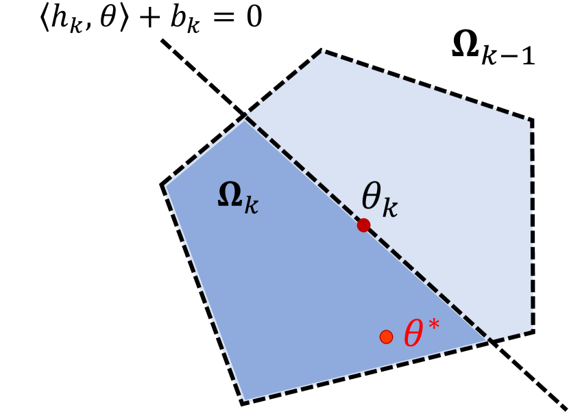
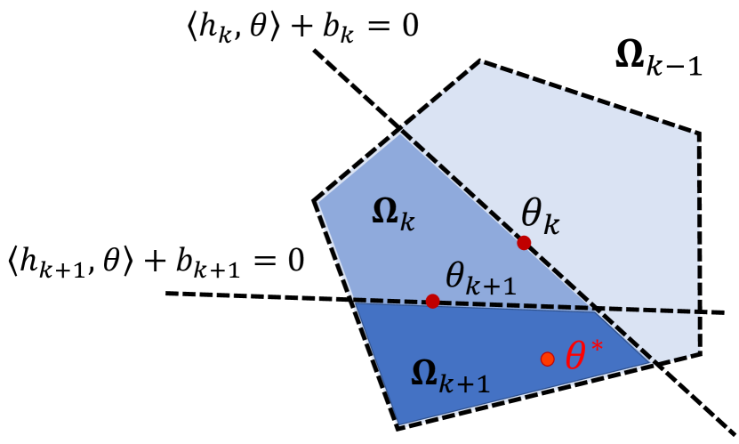
Figure 4: Illustration of updating 𝛀ksubscript𝛀𝑘\boldsymbol{\Omega}_{k}.

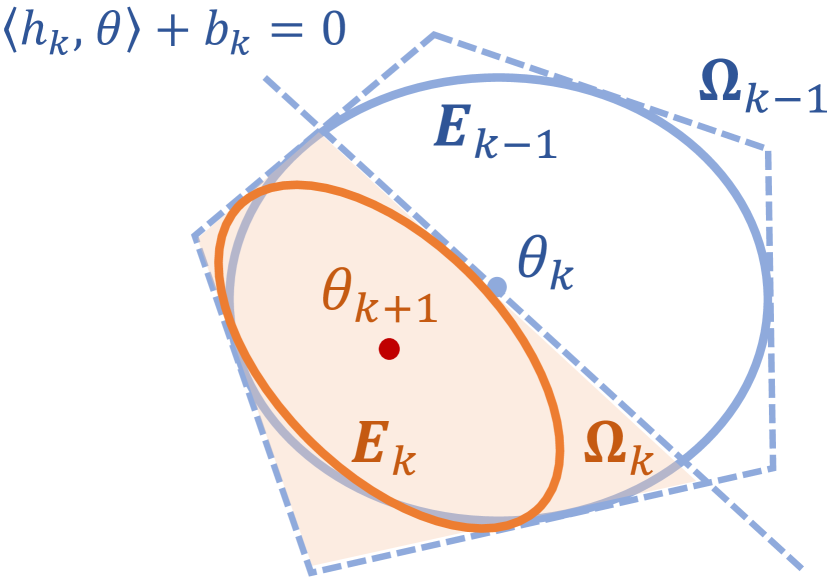
At the k𝑘kth iteration shown in Fig. 4(a), by Step 1 of the main algorithm, a weight vector guess 𝜽ksubscript𝜽𝑘\boldsymbol{\theta}_{k} (red dot) is picked from the current search space 𝛀k1subscript𝛀𝑘1\boldsymbol{\Omega}_{k-1} (light blue region), i.e., 𝜽k𝛀k1subscript𝜽𝑘subscript𝛀𝑘1\boldsymbol{\theta}_{k}\in\boldsymbol{\Omega}_{k-1}. By Step 2, we obtain a hyperplane 𝒉k,𝜽+bk=0subscript𝒉𝑘𝜽subscript𝑏𝑘0\left\langle\boldsymbol{h}_{k},\boldsymbol{\theta}\right\rangle+b_{k}=0 (black dashed line), which cuts through the weight search space 𝛀k1subscript𝛀𝑘1\boldsymbol{\Omega}_{k-1} into two portions. By (25) of Lemma 2, we know that 𝜽ksubscript𝜽𝑘\boldsymbol{\theta}_{k} always lies on this hyperplane because 𝒉k,𝜽k+bk=0subscript𝒉𝑘subscript𝜽𝑘subscript𝑏𝑘0\left\langle\boldsymbol{h}_{k},\boldsymbol{\theta}_{k}\right\rangle+b_{k}=0, as shown in Fig. 4(a). By Step 3 of the main algorithm, we only keep one of the two cut portions, which is the interaction between 𝛀k1subscript𝛀𝑘1\boldsymbol{\Omega}_{k-1} and the half space 𝒉k,𝜽+bk<0subscript𝒉𝑘𝜽subscript𝑏𝑘0\left\langle\boldsymbol{h}_{k},\boldsymbol{\theta}\right\rangle+b_{k}<0, and the kept portion will be used as the new search space for the next iteration, that is, 𝛀k=𝛀k1{𝜽r|𝒉k,𝜽+bk<0}subscript𝛀𝑘subscript𝛀𝑘1conditional-set𝜽superscript𝑟subscript𝒉𝑘𝜽subscript𝑏𝑘0\boldsymbol{\Omega}_{k}=\boldsymbol{\Omega}_{k-1}\cap\left\{\boldsymbol{\theta}\in\mathbb{R}^{r}\,|\,\left\langle\boldsymbol{h}_{k},\boldsymbol{\theta}\right\rangle+b_{k}<0\right\}, as shown by the blue region in Fig. 4(a). The above procedure repeats at the next iteration k+1𝑘1k+1 in Fig. 4(b), and finally produces a smaller search space 𝛀k+1subscript𝛀𝑘1\boldsymbol{\Omega}_{k+1}, as shown by the darkest blue region in Fig. 4(b). From (22), one has 𝛀0𝛀k1𝛀k𝛀k+1superset-of-or-equalssubscript𝛀0subscript𝛀𝑘1superset-of-or-equalssubscript𝛀𝑘superset-of-or-equalssubscript𝛀𝑘1superset-of-or-equals\boldsymbol{\Omega}_{0}\supseteq\cdots\boldsymbol{\Omega}_{k-1}\supseteq\boldsymbol{\Omega}_{k}\supseteq\boldsymbol{\Omega}_{k+1}\supseteq\cdots. Moreover, by (26) in Lemma 2, we note that the true 𝜽superscript𝜽\boldsymbol{\theta}^{*} (red point) is always contained in 𝛀ksubscript𝛀𝑘\boldsymbol{\Omega}_{k} whenever k𝑘k is.

Refer to caption
(a) A large cut from 𝛀k1subscript𝛀𝑘1\boldsymbol{\Omega}_{k-1}
Refer to caption
(b) A small cut from 𝛀k1subscript𝛀𝑘1\boldsymbol{\Omega}_{k-1}
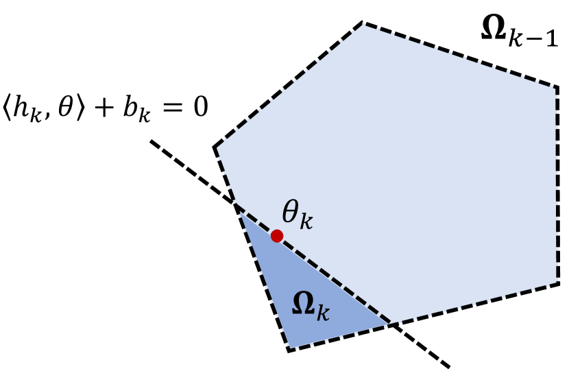
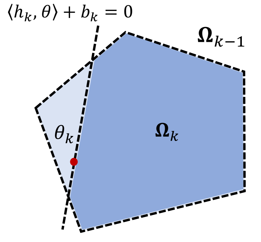
Figure 5: Illustration of how different human directional corrections 𝒂¯ksubscriptbold-¯𝒂𝑘\boldsymbol{\bar{a}}_{k} affect the cut of the weight search space 𝛀k1subscript𝛀𝑘1\boldsymbol{\Omega}_{k-1}.

Besides the above geometric illustration, we also have the following observations:

(1) The key idea of the proposed main algorithm is to cut and remove the weight search space 𝛀k1subscript𝛀𝑘1\boldsymbol{\Omega}_{k-1} as each human directional correction 𝒂¯ksubscriptbold-¯𝒂𝑘\boldsymbol{\bar{a}}_{k} becomes available. Thus, we always expect that 𝛀k1subscript𝛀𝑘1\boldsymbol{\Omega}_{k-1} can quickly shrink as k𝑘k increases, because thereby we can say that the guess 𝜽ksubscript𝜽𝑘\boldsymbol{\theta}_{k} is close to the true weight vector 𝜽superscript𝜽\boldsymbol{\theta}^{*}. As shown in Fig. 4, the reduction rate of 𝛀k1subscript𝛀𝑘1\boldsymbol{\Omega}_{k-1} depends on two factors: the human directional correction 𝒂¯ksubscriptbold-¯𝒂𝑘\boldsymbol{\bar{a}}_{k}, and how to choose 𝜽k𝛀k1subscript𝜽𝑘subscript𝛀𝑘1\boldsymbol{\theta}_{k}\in\boldsymbol{\Omega}_{k-1}, both discussed below.

(2) From (8), we note that human directional correction 𝒂¯ksubscriptbold-¯𝒂𝑘\boldsymbol{\bar{a}}_{k} determines 𝒉ksubscript𝒉𝑘\boldsymbol{h}_{k}, which is the normal vector of the hyperplane 𝒉k,𝜽+bk=0subscript𝒉𝑘𝜽subscript𝑏𝑘0\left\langle\boldsymbol{h}_{k},\boldsymbol{\theta}\right\rangle+b_{k}=0. When fixing 𝜽ksubscript𝜽𝑘\boldsymbol{\theta}_{k}, we can think of the hyperplane rotates around 𝜽ksubscript𝜽𝑘\boldsymbol{\theta}_{k} with different 𝒂¯ksubscriptbold-¯𝒂𝑘\boldsymbol{\bar{a}}_{k}, leading to different removals of 𝛀k1subscript𝛀𝑘1\boldsymbol{\Omega}_{k-1}. This can be illustrated by comparing Fig. 5(a) and Fig. 5(b).

(3) The choice of the guess 𝜽k𝛀k1subscript𝜽𝑘subscript𝛀𝑘1\boldsymbol{\theta}_{k}\in\boldsymbol{\Omega}_{k-1} defines the specific location of the hyperplane 𝒉k,𝜽+bk=0subscript𝒉𝑘𝜽subscript𝑏𝑘0\left\langle\boldsymbol{h}_{k},\boldsymbol{\theta}\right\rangle+b_{k}=0, because the hyperplane is always passing through 𝜽ksubscript𝜽𝑘\boldsymbol{\theta}_{k} by (25) in Lemma 2. Thus, 𝜽ksubscript𝜽𝑘\boldsymbol{\theta}_{k} also affects how 𝛀k1subscript𝛀𝑘1\boldsymbol{\Omega}_{k-1} is cut and removed. This can be illustrated by comparing Fig. 4(a) with Fig. 5(a).

Based on the above observations, we know that the convergence of the proposed main algorithm is determined by the reduction of the weight search space 𝛀k1subscript𝛀𝑘1\boldsymbol{\Omega}_{k-1}. This reduction depends on both the human directional correction 𝒂¯ksubscriptbold-¯𝒂𝑘\boldsymbol{\bar{a}}_{k} and the choice of the weight vector guess 𝜽k𝛀k1subscript𝜽𝑘subscript𝛀𝑘1\boldsymbol{\theta}_{k}\in\boldsymbol{\Omega}_{k-1}. In the next section, we will present a way of choosing 𝜽ksubscript𝜽𝑘\boldsymbol{\theta}_{k} to guarantee the convergence of the proposed main algorithm.

IV Algorithm Implementation and Convergence Analysis

In this section, we detail the choice of 𝜽k𝛀k1subscript𝜽𝑘subscript𝛀𝑘1\boldsymbol{\theta}_{k}\in\boldsymbol{\Omega}_{k-1}, show the convergence of the proposed algorithm, and present a detailed implementation of the algorithm with a termination criterion.

IV-A Choice of Current Guess 𝛉k𝛀k1subscript𝛉𝑘subscript𝛀𝑘1\boldsymbol{\theta}_{k}\in\boldsymbol{\Omega}_{k-1}

In the proposed main algorithm, at iteration k𝑘k, the weight search space 𝛀k1subscript𝛀𝑘1\boldsymbol{\Omega}_{k-1} is updated using (22), rewritten below:

𝛀k=𝛀k1{𝜽r|𝒉k,𝜽+bk<0}.subscript𝛀𝑘subscript𝛀𝑘1conditional-set𝜽superscript𝑟subscript𝒉𝑘𝜽subscript𝑏𝑘0\boldsymbol{\Omega}_{k}=\boldsymbol{\Omega}_{k-1}\cap\left\{\boldsymbol{\theta}\in\mathbb{R}^{r}\,|\,\left\langle\boldsymbol{h}_{k},\boldsymbol{\theta}\right\rangle+b_{k}<0\right\}.

To show the reduction of a weight search space, it is straightforward to use the volume measure (length or area for one- or two-dimension cases, respectively) of a (closure) search space 𝛀ksubscript𝛀𝑘\boldsymbol{\Omega}_{k}, denoted as Vol(𝛀k)Volsubscript𝛀𝑘\operatorname{\text{{Vol}}}(\boldsymbol{\Omega}_{k}). Zero volume implies the convergence of the search space [27]. By (22), we know that 𝛀k𝛀k1subscript𝛀𝑘subscript𝛀𝑘1\boldsymbol{\Omega}_{k}\subseteq\boldsymbol{\Omega}_{k-1} and thus Vol(𝛀k)Volsubscript𝛀𝑘\operatorname{\text{{Vol}}}(\boldsymbol{\Omega}_{k}) is non-increasing. In the following we need to further find a way such that Vol(𝛀k)Volsubscript𝛀𝑘\operatorname{\text{{Vol}}}(\boldsymbol{\Omega}_{k}) is strictly decreasing, i.e., there exists a constant 0α<10𝛼10\leq\alpha<1 such that

Vol(𝛀k)αVol(𝛀k1).Volsubscript𝛀𝑘𝛼Volsubscript𝛀𝑘1\operatorname{\text{{Vol}}}(\boldsymbol{\Omega}_{k})\leq\alpha\operatorname{\text{{Vol}}}(\boldsymbol{\Omega}_{k-1}). (27)

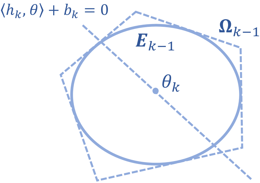
From Fig. 5, we observe that for a fixed choice of 𝜽k𝛀k1subscript𝜽𝑘subscript𝛀𝑘1\boldsymbol{\theta}_{k}\in\boldsymbol{\Omega}_{k-1}, different human directional corrections 𝒂¯ksubscriptbold-¯𝒂𝑘\boldsymbol{\bar{a}}_{k} can lead to different reduction of 𝛀k1subscript𝛀𝑘1\boldsymbol{\Omega}_{k-1}. For example, Fig. 5(a) has a large volume reduction from 𝛀k1subscript𝛀𝑘1\boldsymbol{\Omega}_{k-1} to 𝛀ksubscript𝛀𝑘\boldsymbol{\Omega}_{k} while Fig. 5(b) leads to a very small reduction. Unfortunately, we cannot assume the specific direction of a human correction 𝒂¯ksubscriptbold-¯𝒂𝑘\boldsymbol{\bar{a}}_{k} (it is the discretion of the user), but we can choose the current guess 𝜽ksubscript𝜽𝑘\boldsymbol{\theta}_{k} ‘smartly’ to avoid the very small reduction regardless of specific human corrections. One intuitive choice of such 𝜽ksubscript𝜽𝑘\boldsymbol{\theta}_{k} is at some center of the search space 𝛀k1subscript𝛀𝑘1\boldsymbol{\Omega}_{k-1}. Thus, we define the following center of the maximum volume ellipsoid (MVE) inscribed in 𝛀k1subscript𝛀𝑘1\boldsymbol{\Omega}_{k-1}.

Definition 1 (Maximum Volume Inscribed Ellipsoid [28]).

Given a compact convex set 𝛀r𝛀superscript𝑟\boldsymbol{\Omega}\subset\mathbb{R}^{r}, the maximum volume ellipsoid (MVE) inscribed in 𝛀𝛀\boldsymbol{\Omega}, defined as 𝐄𝐄\boldsymbol{E}, is denoted by

𝑬={B¯𝜽+𝒅¯|𝜽21}.𝑬conditional-set¯𝐵𝜽bold-¯𝒅subscriptdelimited-∥∥𝜽21\boldsymbol{E}=\{\bar{B}\boldsymbol{\theta}+\boldsymbol{\bar{d}}\,|\,\,\lVert\boldsymbol{\theta}\rVert_{2}\leq 1\}. (28)

Here, B¯𝕊++r¯𝐵subscriptsuperscript𝕊𝑟absent\bar{B}\in\mathbb{S}^{r}_{++} (i.e., a r×r𝑟𝑟r\times r positive definite matrix) and 𝐝¯rbold-¯𝐝superscript𝑟\boldsymbol{\bar{d}}\in\mathbb{R}^{r} is called the center of 𝐄𝐄\boldsymbol{E}. B¯¯𝐵\bar{B} and 𝐝¯bold-¯𝐝\boldsymbol{\bar{d}} solve the optimization:

max𝒅,B𝕊++rsubscript𝒅𝐵subscriptsuperscript𝕊𝑟absent\displaystyle\max\nolimits_{\boldsymbol{{d}},{B}\in\mathbb{S}^{r}_{{++}}} logdetB𝐵\displaystyle\log\det{B} (29)
s.t.formulae-sequence𝑠𝑡\displaystyle{s.t.} sup𝜽21I𝛀(B𝜽+𝒅)0,subscriptsupremumsubscriptdelimited-∥∥𝜽21subscriptI𝛀𝐵𝜽𝒅0\displaystyle\sup\nolimits_{\lVert\boldsymbol{\theta}\rVert_{2}\leq 1}\emph{I}_{\boldsymbol{\Omega}}(B\boldsymbol{\theta}+\boldsymbol{d})\leq 0,

where I𝛀(𝛉)=0subscriptI𝛀𝛉0\emph{I}_{\boldsymbol{\Omega}}(\boldsymbol{\theta})=0 for 𝛉𝛀𝛉𝛀\boldsymbol{\theta}\in\boldsymbol{\Omega} and I𝛀(𝛉)=subscriptI𝛀𝛉\emph{I}_{\boldsymbol{\Omega}}(\boldsymbol{\theta})=\infty for 𝛉𝛀𝛉𝛀\boldsymbol{\theta}\notin\boldsymbol{\Omega}.

By Definition 1, let 𝑬ksubscript𝑬𝑘\boldsymbol{E}_{k} denote the MVE inscribed in 𝛀ksubscript𝛀𝑘\boldsymbol{\Omega}_{k} and 𝒅ksubscript𝒅𝑘\boldsymbol{d}_{k} denote the center of 𝑬ksubscript𝑬𝑘\boldsymbol{E}_{k}, k=0,1,𝑘01k=0,1,.... For the choice of 𝜽k+1𝛀ksubscript𝜽𝑘1subscript𝛀𝑘\boldsymbol{\theta}_{k+1}\in\boldsymbol{\Omega}_{k}, we choose

𝜽k+1=𝒅k,subscript𝜽𝑘1subscript𝒅𝑘\boldsymbol{\theta}_{k+1}=\boldsymbol{d}_{k}, (30)

as illustrated in Fig. 6. Other choices of 𝜽k+1subscript𝜽𝑘1\boldsymbol{\theta}_{k+1} using other types of centers of the search space are discussed in Appendix C.
Refer to caption
(a) Center of MVE in 𝛀k1subscript𝛀𝑘1\boldsymbol{\Omega}_{k-1}
Refer to caption
(b) Center of MVE in 𝛀ksubscript𝛀𝑘\boldsymbol{\Omega}_{k}
Figure 6: Illustration of choosing 𝜽k+1subscript𝜽𝑘1\boldsymbol{\theta}_{k+1} as the center of MVE 𝑬ksubscript𝑬𝑘\boldsymbol{E}_{k} inscribed in the weight search space 𝛀ksubscript𝛀𝑘\boldsymbol{\Omega}_{k}.

We now give a computational method to solve for 𝒅ksubscript𝒅𝑘\boldsymbol{d}_{k}, i.e. the center of MVE 𝑬ksubscript𝑬𝑘\boldsymbol{E}_{k} inscribed in 𝛀ksubscript𝛀𝑘\boldsymbol{\Omega}_{k}. Recall that in the main algorithm, the initial 𝛀0subscript𝛀0\boldsymbol{\Omega}_{0} is (21), which is equivalent to

𝛀0={𝜽|𝒆i,𝜽c¯i0𝒆i,𝜽c¯i0,i=1,,r},subscript𝛀0conditional-set𝜽formulae-sequencesubscript𝒆𝑖𝜽subscript¯𝑐𝑖0subscript𝒆𝑖𝜽subscript¯𝑐𝑖0𝑖1𝑟\boldsymbol{\Omega}_{0}=\left\{\boldsymbol{\theta}\,\,\,\middle\rvert\,\,\begin{aligned} \left\langle\boldsymbol{e}_{i},\boldsymbol{\theta}\right\rangle-\bar{c}_{i}\leq 0\\ -\left\langle\boldsymbol{e}_{i},\boldsymbol{\theta}\right\rangle-\underaccent{\bar}{c}_{i}\leq 0\end{aligned},\,\,\,\,\,i=1,\cdots,r\right\}, (31)

where 𝒆isubscript𝒆𝑖\boldsymbol{e}_{i} is a unit vector with the only i𝑖ith entry as 1. Following the update (22), 𝛀ksubscript𝛀𝑘\boldsymbol{\Omega}_{k} is also a compact polytope, which is

𝛀k={𝜽|𝒆i,𝜽c¯i0,i=1,,r;𝒆i,𝜽c¯i0,i=1,,r;𝒉j,𝜽+bj<0,j=1,,k}.subscript𝛀𝑘conditional-set𝜽missing-subexpressionformulae-sequencesubscript𝒆𝑖𝜽subscript¯𝑐𝑖0𝑖1𝑟missing-subexpressionformulae-sequencesubscript𝒆𝑖𝜽subscript¯𝑐𝑖0𝑖1𝑟missing-subexpressionformulae-sequencesubscript𝒉𝑗𝜽subscript𝑏𝑗0𝑗1𝑘\boldsymbol{\Omega}_{k}=\left\{\boldsymbol{\theta}\,\middle\rvert\,\begin{aligned} &\left\langle\boldsymbol{e}_{i},\boldsymbol{\theta}\right\rangle-\bar{c}_{i}\leq 0,\,\,i=1,\cdots,r;\\ &-\left\langle\boldsymbol{e}_{i},\boldsymbol{\theta}\right\rangle-\underaccent{\bar}{c}_{i}\leq 0,\,\,i=1,\cdots,r;\\ &\left\langle\boldsymbol{h}_{j},\boldsymbol{\theta}\right\rangle+b_{j}<0,\,\,j=1,\cdots,k\end{aligned}\right\}. (32)

As a result, solving (29) for the center 𝒅ksubscript𝒅𝑘\boldsymbol{d}_{k} becomes a convex program [28], stated in the lemma below.

Lemma 3.

For a polytope 𝛀ksubscript𝛀𝑘\boldsymbol{\Omega}_{k} in (32), the center 𝐝ksubscript𝐝𝑘\boldsymbol{d}_{k} of the MVE 𝐄ksubscript𝐄𝑘\boldsymbol{E}_{k} inscribed in 𝛀ksubscript𝛀𝑘\boldsymbol{\Omega}_{k} can be solved via the following convex optimization:

min𝒅,B𝕊++rsubscript𝒅𝐵subscriptsuperscript𝕊𝑟absent\displaystyle\min\nolimits_{\boldsymbol{d},B\in\mathbb{S}^{r}_{{++}}} logdetB𝐵\displaystyle-\log\det{B} (33)
s.t.formulae-sequence𝑠𝑡\displaystyle{s.t.} B𝒆i2+𝒅,𝒆ic¯i,i=1,r,formulae-sequencesubscriptdelimited-∥∥𝐵subscript𝒆𝑖2𝒅subscript𝒆𝑖subscript¯𝑐𝑖𝑖1𝑟\displaystyle\,\,\lVert B\boldsymbol{e}_{i}\rVert_{2}+\left\langle\boldsymbol{d},\boldsymbol{e}_{i}\right\rangle\leq\bar{c}_{i},\,\,i{=}1,\cdots r,
B𝒆i2𝒅,𝒆ic¯i,i=1,r,formulae-sequencesubscriptdelimited-∥∥𝐵subscript𝒆𝑖2𝒅subscript𝒆𝑖subscript¯𝑐𝑖𝑖1𝑟\displaystyle\,\,\lVert B\boldsymbol{e}_{i}\rVert_{2}-\left\langle\boldsymbol{d},\boldsymbol{e}_{i}\right\rangle\leq\underaccent{\bar}{c}_{i},\,\,i{=}1,\cdots r,
B𝒉j2+𝒅,𝒉jbj,j=1,k.formulae-sequencesubscriptdelimited-∥∥𝐵subscript𝒉𝑗2𝒅subscript𝒉𝑗subscript𝑏𝑗𝑗1𝑘\displaystyle\,\,\lVert B\boldsymbol{{h}}_{j}\rVert_{2}{+}\left\langle\boldsymbol{d},\boldsymbol{h}_{j}\right\rangle\leq-b_{j},\,\,j{=}1,\cdots k.

The proof of Lemma 3 can be found in Chapter 8.4.2 in [28, pp.414]. (33) can be efficiently solved by available convex program solvers, e.g., [29]. In the implementation, since the number of linear inequalities grows as k𝑘k increases, the trick of dropping some redundant inequalities in (32) can be adopted [27]. Dropping redundant inequalities does not change 𝛀ksubscript𝛀𝑘\boldsymbol{\Omega}_{k} and its volume reduction (convergence). Please see how to identify the redundant inequalities in [27].

IV-B Exponential Convergence and Termination Criterion

Now we analyze the convergence of the volume reduction of 𝛀ksubscript𝛀𝑘\boldsymbol{\Omega}_{k} and develop its termination criterion in implementation. First, the convergence of the reduction of Vol(𝛀k)Volsubscript𝛀𝑘\operatorname{\text{{Vol}}}(\boldsymbol{\Omega}_{k}) is guaranteed by the following lemma.

Lemma 4.

Let 𝛉ksubscript𝛉𝑘\boldsymbol{\theta}_{k} be chosen as the center 𝐝k1subscript𝐝𝑘1\boldsymbol{d}_{k-1} of the MVE 𝐄k1subscript𝐄𝑘1\boldsymbol{E}_{k-1} inscribed in 𝛀k1rsubscript𝛀𝑘1superscript𝑟\boldsymbol{\Omega}_{k-1}\subset\mathbb{R}^{r}. Then, the update (22) has

Vol(𝛀k)Vol(𝛀k1)(11r).Volsubscript𝛀𝑘Volsubscript𝛀𝑘111𝑟\frac{\operatorname{\text{{Vol}}}({\boldsymbol{\Omega}_{k}})}{\operatorname{\text{{Vol}}}(\boldsymbol{\Omega}_{k-1})}\leq(1-\frac{1}{r}). (34)

Lemma 4 is a theorem directly from [30]. Lemma 4 indicates

Vol(𝛀k)(11r)kVol(𝛀0).Volsubscript𝛀𝑘superscript11𝑟𝑘Volsubscript𝛀0\operatorname{\text{{Vol}}}{(\boldsymbol{\Omega}_{k})}\leq(1-\frac{1}{r})^{k}\operatorname{\text{{Vol}}}{(\boldsymbol{\Omega}_{0})}.

Thus, the convergence rate of Vol(𝛀k)0Volsubscript𝛀𝑘0\operatorname{\text{{Vol}}}{(\boldsymbol{\Omega}_{k})}\rightarrow 0 is as fast as (11r)k0superscript11𝑟𝑘0(1-\frac{1}{r})^{k}\rightarrow 0, as k=0,1,2,𝑘012k=0,1,2,....

To implement the proposed main algorithm, we will not only need the exponential convergence as established by Lemma 4 but also a termination criterion, which specifies the maximum number of iterations needed for Vol(𝛀k)Volsubscript𝛀𝑘\operatorname{\text{{Vol}}}{(\boldsymbol{\Omega}_{k})} below certain a given threshold. Thus, we have the following theorem.

Theorem 1.

In the main algorithm, suppose 𝛀0subscript𝛀0\boldsymbol{\Omega}_{0} is given by (21), and at iteration k𝑘k, 𝛉ksubscript𝛉𝑘\boldsymbol{\theta}_{k} is chosen as the center 𝐝k1subscript𝐝𝑘1\boldsymbol{d}_{k-1} of the MVE 𝐄k1subscript𝐄𝑘1\boldsymbol{E}_{k-1} inscribed in 𝛀k1subscript𝛀𝑘1\boldsymbol{\Omega}_{k-1}. Given a termination condition

Vol(𝛀k)(2ϵ)rVolsubscript𝛀𝑘superscript2italic-ϵ𝑟\operatorname{\text{{Vol}}}{(\boldsymbol{\Omega}_{k})}\leq(2\epsilon)^{r}

with ϵitalic-ϵ\epsilon a user-specified threshold, the proposed main algorithm runs for kK𝑘𝐾k\leq K iterations, namely, the algorithm terminates in at most K𝐾K iterations, where

K=rlog(R/ϵ)log(11/r),𝐾𝑟𝑅italic-ϵ11𝑟K=\frac{r\log(R/\epsilon)}{-\log(1-1/r)}, (35)

with R𝑅R given in (24).

Proof.

Initially, we have Vol(𝛀0)(2R)rVolsubscript𝛀0superscript2𝑅𝑟\operatorname{\text{{Vol}}}{(\boldsymbol{\Omega}_{0})}\leq(2R)^{r}. From Lemma 4, after k𝑘k iterations, we have

Vol(𝛀k)(11r)kVol(𝛀0)(11r)k(2R)r,Volsubscript𝛀𝑘superscript11𝑟𝑘Volsubscript𝛀0superscript11𝑟𝑘superscript2𝑅𝑟\operatorname{\text{{Vol}}}{(\boldsymbol{\Omega}_{k})}\leq(1-\frac{1}{r})^{k}\operatorname{\text{{Vol}}}{(\boldsymbol{\Omega}_{0})}\leq(1-\frac{1}{r})^{k}(2R)^{r}, (36)

which yields to

logVol(𝛀k)klog(11r)+log(2R)r.\log\operatorname{\text{{Vol}}}{(\boldsymbol{\Omega}_{k})}\leq k\log(1-\frac{1}{r})+\log(2R)^{r}. (37)

When k=rlog(R/ϵ)log(11/r)𝑘𝑟𝑅italic-ϵ11𝑟k=\frac{r\log(R/\epsilon)}{-\log(1-1/r)},

logVol(𝛀k)rlog(R/ϵ)+log(2R)r.\log\operatorname{\text{{Vol}}}{(\boldsymbol{\Omega}_{k})}\leq-r\log(R/\epsilon)+\log(2R)^{r}. (38)

The above equation is simplified to

logVol(𝛀k)log(2ϵ)r,\log\operatorname{\text{{Vol}}}{(\boldsymbol{\Omega}_{k})}\leq\log(2\epsilon)^{r}, (39)

which means that the termination condition Vol(𝛀k)(2ϵ)rVolsubscript𝛀𝑘superscript2italic-ϵ𝑟\operatorname{\text{{Vol}}}{(\boldsymbol{\Omega}_{k})}\leq(2\epsilon)^{r} is satisfied. This completes the proof. ∎

We have the following comments on the above Theorem 1.

Remark 5.

Since Lemma 2 states that both 𝛉superscript𝛉\boldsymbol{\theta}^{*} and 𝛉ksubscript𝛉𝑘\boldsymbol{\theta}_{k} are in 𝛀ksubscript𝛀𝑘\boldsymbol{\Omega}_{k} for any k=1,2,3,𝑘123k=1,2,3,... , the user-specified threshold ϵitalic-ϵ\epsilon in the termination condition Vol(𝛀k)(2ϵ)rVolsubscript𝛀𝑘superscript2italic-ϵ𝑟\operatorname{\text{{Vol}}}{(\boldsymbol{\Omega}_{k})}\leq(2\epsilon)^{r} can also be understood as an indicator for the distance between the true 𝛉superscript𝛉\boldsymbol{\theta}^{*} (usually unknown in practice) and the robot current guess 𝛉ksubscript𝛉𝑘\boldsymbol{\theta}_{k}. ϵitalic-ϵ\epsilon is set based on the desired learning accuracy. 111In practice, it is usually easy to set ϵitalic-ϵ\epsilon with a small value, because the empirical results in Sections VI and VII show that the robot motion trajectory can converge (to the desired motion) more quickly than the objective function itself. This means that one usually sees the convergence of the robot trajectory before the termination condition is reached, as shown in Fig. 10. More discussion about setting ϵitalic-ϵ\epsilon will be given in Appendix B-D.

IV-C Detailed Implementation of Main Algorithm

With the termination criterion stated in Theorem 1 and the choice of 𝜽ksubscript𝜽𝑘\boldsymbol{\theta}_{k} in (30) and Lemma 3, we present the detailed implementation of the proposed main method in Algorithm 1. The setting of the initial 𝛀0subscript𝛀0\boldsymbol{\Omega}_{0} in (21) and ϵitalic-ϵ\epsilon will be given in Appendix B-D.

Input: Specify a termination threshold ϵitalic-ϵ\epsilon and use it to compute the maximum iteration K𝐾K by (35).
Initialization: Initial weight search space 𝛀0subscript𝛀0\boldsymbol{\Omega}_{0} in (21).
for k=1,2,,K𝑘12𝐾k=1,2,\cdots,K do
      
      Choose a weight vector guess 𝜽k𝛀k1subscript𝜽𝑘subscript𝛀𝑘1\boldsymbol{\theta}_{k}\in\boldsymbol{\Omega}_{k-1} via Lemma 3;
      
      Restart and plan a robot trajectory 𝝃𝜽ksubscript𝝃subscript𝜽𝑘\boldsymbol{\xi}_{\boldsymbol{\theta}_{k}} by solving a trajectory optimization with the cost function J(𝜽k)𝐽subscript𝜽𝑘J(\boldsymbol{\theta}_{k}) in (2) and the dynamics in (1);
      
      Robot executes the planned trajectory 𝝃𝜽ksubscript𝝃subscript𝜽𝑘\boldsymbol{\xi}_{\boldsymbol{\theta}_{k}} while receving the human averaged directional correction 𝒂¯ksubscriptbold-¯𝒂𝑘\boldsymbol{\bar{a}}_{k} in (6b);
      
      Compute the matrices 𝑯1(𝒙0:T+1𝜽k,𝒖0:T𝜽k)subscript𝑯1subscriptsuperscript𝒙subscript𝜽𝑘:0𝑇+1subscriptsuperscript𝒖subscript𝜽𝑘:0𝑇\boldsymbol{H}_{1}(\boldsymbol{x}^{\boldsymbol{\theta}_{k}}_{0:T\text{+}1},\boldsymbol{u}^{\boldsymbol{\theta}_{k}}_{0:T}) and 𝑯2(𝒙0:T+1𝜽k,𝒖0:T𝜽k)subscript𝑯2subscriptsuperscript𝒙subscript𝜽𝑘:0𝑇+1subscriptsuperscript𝒖subscript𝜽𝑘:0𝑇\boldsymbol{H}_{2}(\boldsymbol{x}^{\boldsymbol{\theta}_{k}}_{0:T\text{+}1},\boldsymbol{u}^{\boldsymbol{\theta}_{k}}_{0:T}), and then compute the hyperplane and half space 𝒉k,𝜽+bk<0subscript𝒉𝑘𝜽subscript𝑏𝑘0\left\langle\boldsymbol{h}_{k},\boldsymbol{\theta}\right\rangle+b_{k}<0 via (7)-(8);
      
      Update the weight search space by 𝛀k=𝛀k1{𝜽r|𝒉k,𝜽+bk<0}subscript𝛀𝑘subscript𝛀𝑘1conditional-set𝜽superscript𝑟subscript𝒉𝑘𝜽subscript𝑏𝑘0\boldsymbol{\Omega}_{k}=\boldsymbol{\Omega}_{k-1}\cap\left\{\boldsymbol{\theta}\in\mathbb{R}^{r}\,|\,\left\langle\boldsymbol{h}_{k},\boldsymbol{\theta}\right\rangle+b_{k}<0\right\} via (22);
      
end for
Output: 𝜽Ksubscript𝜽𝐾\boldsymbol{\theta}_{K}.
Algorithm 1 Learning from directional corrections

V Numerical Examples

In this section, we will test the proposed method in numerical simulations and make comparisons with the magnitude-correction methods discussed in the previous related work.

V-A Inverted Pendulum

The dynamics of a pendulum is

α¨=glsinαdml2α˙+uml2,¨𝛼𝑔𝑙𝛼𝑑𝑚superscript𝑙2˙𝛼𝑢𝑚superscript𝑙2\ddot{\alpha}=\frac{-g}{l}\sin\alpha-\frac{d}{ml^{2}}\dot{\alpha}+\frac{u}{ml^{2}}, (40)

with α𝛼\alpha being the angle between the pendulum and the direction of gravity, u𝑢u is the torque applied to the pivot, l=1𝑙1l=1m, m=1𝑚1m=1kg, and d=0.1𝑑0.1d=0.1Ns/m are the length, mass, and damping ratio of the pendulum, respectively. We discretize the dynamics using the Euler method with a time interval Δ=0.2Δ0.2\Delta=0.2s. The state and control input of the pendulum are 𝒙=[α,α˙]𝖳𝒙superscript𝛼˙𝛼𝖳\boldsymbol{x}=[\alpha,\dot{\alpha}]^{\mkern-1.5mu\mathsf{T}} and 𝒖=u𝒖𝑢\boldsymbol{u}=u, respectively. The initial condition is 𝒙0=[0,0]𝖳subscript𝒙0superscript00𝖳\boldsymbol{x}_{0}=[0,0]^{\mkern-1.5mu\mathsf{T}}. In the cost function (2), we set the feature and weight vectors as

ϕbold-italic-ϕ\displaystyle\boldsymbol{\phi} =[α2,α,α˙2,u2]𝖳4,absentsuperscriptsuperscript𝛼2𝛼superscript˙𝛼2superscript𝑢2𝖳superscript4\displaystyle=[\alpha^{2},\alpha,\dot{\alpha}^{2},u^{2}]^{\mkern-1.5mu\mathsf{T}}\in\mathbb{R}^{4}, (41)
𝜽𝜽\displaystyle\boldsymbol{\theta} =[θ1,θ2,θ3,θ4]𝖳4,absentsuperscriptsubscript𝜃1subscript𝜃2subscript𝜃3subscript𝜃4𝖳superscript4\displaystyle=[\theta_{1},\theta_{2},\theta_{3},\theta_{4}]^{\mkern-1.5mu\mathsf{T}}\in\mathbb{R}^{4},

respectively, and the final cost h(𝒙T+1)=10(απ)2+10α˙2subscript𝒙𝑇110superscript𝛼𝜋210superscript˙𝛼2h(\boldsymbol{x}_{T+1})=10(\alpha-\pi)^{2}+10\dot{\alpha}^{2}, as our goal is to swing up the pendulum. The discrete time horizon is T=30𝑇30T=30.

For numerical analysis, we ‘simulate’ the human directional corrections instead of using real human corrections. The simulated corrections are generated as follows. Suppose that the true weight vector is known: 𝜽=[0.5,0.5,0.5,0.5]𝖳superscript𝜽superscript0.50.50.50.5𝖳\boldsymbol{\theta}^{*}{=}[0.5,0.5,0.5,0.5]^{\mkern-1.5mu\mathsf{T}}. At iteration k𝑘k, a simulated correction 𝒂tksubscript𝒂subscript𝑡𝑘\boldsymbol{a}_{t_{k}} is generated using the sign of the gradient of the true cost function J(𝜽)𝐽superscript𝜽J(\boldsymbol{\theta}^{*}), i.e.,

𝒂tk=sign(J(𝒖0:T𝜽k,𝜽)[tk]).subscript𝒂subscript𝑡𝑘sign𝐽subscriptsuperscript𝒖subscript𝜽𝑘:0𝑇superscript𝜽delimited-[]subscript𝑡𝑘\boldsymbol{a}_{t_{k}}=-\text{sign}\left(\nabla J(\boldsymbol{u}^{\boldsymbol{\theta}_{k}}_{0:T},\boldsymbol{\theta}^{*})\left[{t_{k}}\right]\right)\in\mathbb{R}. (42)

Here, J(𝒖0:T𝜽k,𝜽)[tk]𝐽subscriptsuperscript𝒖subscript𝜽𝑘:0𝑇superscript𝜽delimited-[]subscript𝑡𝑘\nabla J(\boldsymbol{u}^{\boldsymbol{\theta}_{k}}_{0:T},\boldsymbol{\theta}^{*})\left[{t_{k}}\right] denotes the tksubscript𝑡𝑘t_{k}th entry of J𝐽\nabla J, and the correction time tksubscript𝑡𝑘{t_{k}} is randomly drawn from the a uniform distribution over horizon [0,T]0𝑇[0,T]. Obviously, the above simulated directional corrections satisfies the assumption (4).
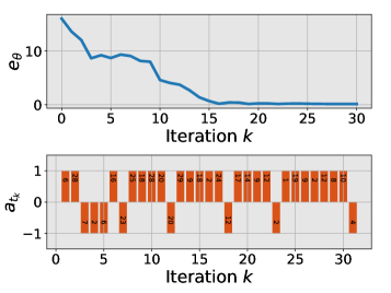
Refer to caption
Figure 7: Learning from simulated directional corrections for the pendulum. The upper panel shows the weight error e𝜽=𝜽𝜽2subscript𝑒𝜽superscriptdelimited-∥∥𝜽superscript𝜽2e_{\boldsymbol{\theta}}=\lVert\boldsymbol{\theta}-\boldsymbol{\theta}^{*}\rVert^{2} versus iteration. The bottom shows the simulated directional correction 𝒂tksubscript𝒂subscript𝑡𝑘\boldsymbol{a}_{t_{k}} (positive or negative sign) at each iteration k𝑘{k}; here, the value in each bar is tksubscript𝑡𝑘{t}_{k}, which is randomly drawn from a uniform distribution over horizon [0,30]030[0,30].

The initial weight search space is set as 𝛀0={𝜽| 0𝜽[i]5,i=1,2,3,4}subscript𝛀0conditional-set𝜽formulae-sequence 0𝜽delimited-[]𝑖5𝑖1234\boldsymbol{\Omega}_{0}=\{\boldsymbol{\theta}\,|\,0\leq{\boldsymbol{\theta}[i]}\leq 5,\,\,i=1,2,3,4\}. In Algorithm 1, we set the termination threshold ϵ=101italic-ϵsuperscript101\epsilon=10^{-1}, and the maximum learning iteration solved via (35) is K=55𝐾55K=55. We apply Algorithm 1 to learn the true 𝜽superscript𝜽\boldsymbol{\theta}^{*}. To illustrate results, we define the weight error e𝜽=𝜽𝜽2subscript𝑒𝜽superscriptdelimited-∥∥𝜽superscript𝜽2e_{\boldsymbol{\theta}}=\lVert\boldsymbol{\theta}-\boldsymbol{\theta}^{*}\rVert^{2} and plot e𝜽subscript𝑒𝜽e_{\boldsymbol{\theta}} versus iteration k𝑘k in the top panel of Fig. 7. In the bottom panel of Fig. 7, we plot the simulated directional correction 𝒂tksubscript𝒂subscript𝑡𝑘\boldsymbol{a}_{t_{k}} at each iteration k𝑘k, where +11+1 and 11-1 bar denote the positive and negative sign (i.e., direction) of correction 𝒂tksubscript𝒂subscript𝑡𝑘\boldsymbol{a}_{t_{k}} in (42), respectively; the number inside the bar denotes the correction time tksubscript𝑡𝑘{t_{k}} randomly drawn from [0,T]0𝑇[0,T].

From the results in Fig. 7, we can see that as the learning iteration k𝑘k increases, the weight vector guess 𝜽ksubscript𝜽𝑘\boldsymbol{\theta}_{k} converges to the true 𝜽=[0.5,0.5,0.5,0.5]𝖳superscript𝜽superscript0.50.50.50.5𝖳\boldsymbol{\theta}^{*}=[0.5,0.5,0.5,0.5]^{\mkern-1.5mu\mathsf{T}}. This shows the efficacy of the method, as guaranteed by Theorem 1.

V-B Two-link Robot Arm System

Here, we test the proposed method on a two-link robot arm. The dynamics of the robot arm system (moving horizontally) is M(𝒒)𝒒¨+𝒄(𝒒,𝒒˙)=𝝉𝑀𝒒¨𝒒𝒄𝒒bold-˙𝒒𝝉M(\boldsymbol{q})\ddot{\boldsymbol{q}}+\boldsymbol{c}(\boldsymbol{q},\boldsymbol{\dot{q}})=\boldsymbol{\tau}, where M(𝒒)𝑀𝒒M(\boldsymbol{q}) is the inertia matrix, 𝒄(𝒒,𝒒˙)𝒄𝒒bold-˙𝒒\boldsymbol{c}(\boldsymbol{q},\boldsymbol{\dot{q}}) is the Coriolis and centrifugal term; 𝒒=[q1,q2]𝖳𝒒superscriptsubscript𝑞1subscript𝑞2𝖳\boldsymbol{q}=[q_{1},q_{2}]^{\mkern-1.5mu\mathsf{T}} is the vector of joint angles, and 𝝉=[τ1,τ2]𝖳𝝉superscriptsubscript𝜏1subscript𝜏2𝖳\boldsymbol{\tau}=[\tau_{1},\tau_{2}]^{\mkern-1.5mu\mathsf{T}} is the vector of joint toques. The state and control input are 𝒙=[𝒒,𝒒˙]𝖳4𝒙superscript𝒒˙𝒒𝖳superscript4\boldsymbol{x}=[\boldsymbol{q},\dot{\boldsymbol{q}}]^{\mkern-1.5mu\mathsf{T}}\in\mathbb{R}^{4} and 𝒖=𝝉2𝒖𝝉superscript2\boldsymbol{u}=\boldsymbol{\tau}\in\mathbb{R}^{2}, respectively. The initial condition of the robot arm is set as 𝒙0=[0,0,0,0]𝖳subscript𝒙0superscript0000𝖳\boldsymbol{x}_{0}=[0,0,0,0]^{\mkern-1.5mu\mathsf{T}}. All physical parameters in the dynamics are units. We discretize the dynamics using the Euler method with a time interval Δ=0.2Δ0.2\Delta=0.2s. In the cost function (2), we set the feature and weight vectors as

ϕbold-italic-ϕ\displaystyle\boldsymbol{\phi} =[q12,q1,q22,q2,𝒖2]𝖳5,absentsuperscriptsuperscriptsubscript𝑞12subscript𝑞1superscriptsubscript𝑞22subscript𝑞2superscriptdelimited-∥∥𝒖2𝖳superscript5\displaystyle=[q_{1}^{2},\,q_{1},\,{q}_{2}^{2},\,{q}_{2},\,\lVert\boldsymbol{u}\rVert^{2}]^{\mkern-1.5mu\mathsf{T}}\in\mathbb{R}^{5}, (43a)
𝜽𝜽\displaystyle\boldsymbol{\theta} =[θ1,θ2,θ3,θ4,θ5]𝖳5,absentsuperscriptsubscript𝜃1subscript𝜃2subscript𝜃3subscript𝜃4subscript𝜃5𝖳superscript5\displaystyle=[\theta_{1},\theta_{2},\theta_{3},\theta_{4},\theta_{5}]^{\mkern-1.5mu\mathsf{T}}\in\mathbb{R}^{5}, (43b)

respectively, and the final cost h(𝒙T+1)=100((q1π2)2+q22+q˙12+q˙22)subscript𝒙𝑇1100superscriptsubscript𝑞1𝜋22superscriptsubscript𝑞22superscriptsubscript˙𝑞12superscriptsubscript˙𝑞22h(\boldsymbol{x}_{T+1})=100\big{(}(q_{1}-\frac{\pi}{2})^{2}+q_{2}^{2}+\dot{q}_{1}^{2}+\dot{q}_{2}^{2}\big{)}, as the robot arm aims to reach and stop at the pose of 𝒒=[π2,0]𝖳𝒒superscript𝜋20𝖳\boldsymbol{q}=[\frac{\pi}{2},0]^{\mkern-1.5mu\mathsf{T}}. The discrete-time horizon is T=50𝑇50T=50.

We still ‘simulate’ directional corrections. Suppose that we know the true 𝜽=[1,1,1,1,1]𝖳superscript𝜽superscript11111𝖳\boldsymbol{\theta}^{*}=[1,1,1,1,1]^{\mkern-1.5mu\mathsf{T}}. At each iteration k𝑘k, the simulation generates a directional correction 𝒂tksubscript𝒂subscript𝑡𝑘\boldsymbol{a}_{t_{k}} using the sign of gradient of the true J(𝜽)𝐽superscript𝜽J(\boldsymbol{\theta}^{*}):

𝒂tk=sign(J(𝒖0:T𝜽k,𝜽)[2tk:2tk+1])2,\boldsymbol{a}_{t_{k}}=-\text{sign}\left(\nabla J(\boldsymbol{u}^{\boldsymbol{\theta}_{k}}_{0:T},\boldsymbol{\theta}^{*})\left[{2t_{k}:2t_{k}+1}\right]\right)\in\mathbb{R}^{2}, (44)

where J(𝒖0:T𝜽k,𝜽)[2tk:2tk+1]\nabla J(\boldsymbol{u}^{\boldsymbol{\theta}_{k}}_{0:T},\boldsymbol{\theta}^{*})\left[{2t_{k}:2t_{k}+1}\right] are the entries at the locations from 2tk2subscript𝑡𝑘2t_{k} to 2tk+12subscript𝑡𝑘12t_{k}+1 in J𝐽\nabla J (because 𝒖2𝒖superscript2\boldsymbol{u}\in\mathbb{R}^{2}), and the correction time tksubscript𝑡𝑘t_{k} is randomly drawn from (uniform distribution) time horizon [0,T]0𝑇[0,T]. sign is applied entry-wise.

Refer to caption
Figure 8: Learning from simulated directional corrections for the robot arm. The plot is e𝜽=𝜽𝜽2subscript𝑒𝜽superscriptdelimited-∥∥𝜽superscript𝜽2e_{\boldsymbol{\theta}}=\lVert\boldsymbol{\theta}-\boldsymbol{\theta}^{*}\rVert^{2} versus iteration. The corrections are given in Fig. 9.

The initial weight search space is 𝛀0={𝜽|  0𝜽[i]4,i=1,2,,5}subscript𝛀0conditional-set𝜽formulae-sequence  0𝜽delimited-[]𝑖4𝑖125\boldsymbol{\Omega}_{0}=\{\boldsymbol{\theta}\,\,|\,\,0\leq\boldsymbol{\theta}[i]\leq 4,\,\,\,i=1,2,...,5\}. We set the termination threshold ϵ=101italic-ϵsuperscript101\epsilon=10^{-1}, and the maximum learning iteration is K=83𝐾83K=83 by (35). We apply Algorithm 1 to learn the true 𝜽superscript𝜽\boldsymbol{\theta}^{*}. We define the weight error e𝜽=𝜽𝜽2subscript𝑒𝜽superscriptdelimited-∥∥𝜽superscript𝜽2e_{\boldsymbol{\theta}}=\lVert\boldsymbol{\theta}-\boldsymbol{\theta}^{*}\rVert^{2} and plot e𝜽subscript𝑒𝜽e_{\boldsymbol{\theta}} versus iteration in Fig. 8. We also plot 𝒂tk=[atk,1,atk,2]𝖳subscript𝒂subscript𝑡𝑘superscriptsubscript𝑎subscript𝑡𝑘1subscript𝑎subscript𝑡𝑘2𝖳\boldsymbol{a}_{t_{k}}=[a_{t_{k},1},a_{t_{k},2}]^{\mkern-1.5mu\mathsf{T}} at each iteration k𝑘k in Fig. 9, where the value labeled on each bar marks the correction time tksubscript𝑡𝑘t_{k}. The results in Fig. 8 show that as the iteration increases, 𝜽ksubscript𝜽𝑘\boldsymbol{\theta}_{k} converges to the true 𝜽superscript𝜽\boldsymbol{\theta}^{*}, which again confirms Theorem 1.

Refer to caption
Figure 9: Simulated directional correction 𝒂tk=[atk,1,atk,2]𝖳subscript𝒂subscript𝑡𝑘superscriptsubscript𝑎subscript𝑡𝑘1subscript𝑎subscript𝑡𝑘2𝖳\boldsymbol{a}_{t_{k}}=[a_{t_{k},1},a_{t_{k},2}]^{\mkern-1.5mu\mathsf{T}} at each iteration k𝑘k for the robot arm. The number inside the bar is the correction time tksubscript𝑡𝑘{t}_{k} randomly drawn from range [0,50]050[0,50].

V-C Comparison with Magnitude-Correction Methods

We compare the proposed method with two related works [6, 7], both of which learn an objective function from magnitude corrections. The comparison is conducted on the inverted pendulum used in Section V-A. According to [7], given a magnitude correction, the trajectory deformation [8] is used to obtain a human intended trajectory. Specifically, suppose the robot trajectory is 𝝃𝜽k={𝒙0:T+1𝜽k,𝒖0:T𝜽k}subscript𝝃subscript𝜽𝑘subscriptsuperscript𝒙subscript𝜽𝑘:0𝑇1subscriptsuperscript𝒖subscript𝜽𝑘:0𝑇\boldsymbol{{\xi}}_{\boldsymbol{\theta}_{k}}=\{\boldsymbol{{x}}^{\boldsymbol{\theta}_{k}}_{0:T+1},\boldsymbol{{u}}^{\boldsymbol{\theta}_{k}}_{0:T}\}. Given a correction 𝒂¯ksubscriptbold-¯𝒂𝑘\boldsymbol{\bar{a}}_{k}, the human intended trajectory, denoted as 𝝃¯𝜽k={𝒙¯0:T+1𝜽k,𝒖¯0:T𝜽k}subscriptbold-¯𝝃subscript𝜽𝑘subscriptsuperscriptbold-¯𝒙subscript𝜽𝑘:0𝑇1subscriptsuperscriptbold-¯𝒖subscript𝜽𝑘:0𝑇\boldsymbol{\bar{\xi}}_{\boldsymbol{\theta}_{k}}=\{\boldsymbol{\bar{x}}^{\boldsymbol{\theta}_{k}}_{0:T+1},\boldsymbol{\bar{u}}^{\boldsymbol{\theta}_{k}}_{0:T}\}, is solved as

𝒖¯0:T𝜽k=𝒖0:T𝜽k+M1𝒂¯k,subscriptsuperscriptbold-¯𝒖subscript𝜽𝑘:0𝑇subscriptsuperscript𝒖subscript𝜽𝑘:0𝑇superscript𝑀1subscriptbold-¯𝒂𝑘\boldsymbol{\bar{u}}^{\boldsymbol{\theta}_{k}}_{0:T}=\boldsymbol{{u}}^{\boldsymbol{\theta}_{k}}_{0:T}+M^{-1}\boldsymbol{\bar{a}}_{k}, (45)

where M𝑀M is a matrix to propagate a single-time-step correction 𝒂¯ksubscriptbold-¯𝒂𝑘\boldsymbol{\bar{a}}_{k} (5) along the rest of the robot trajectory [22], and 𝒙¯0:T+1𝜽ksubscriptsuperscriptbold-¯𝒙subscript𝜽𝑘:0𝑇1\boldsymbol{\bar{x}}^{\boldsymbol{\theta}_{k}}_{0:T+1} in 𝝃¯𝜽ksubscriptbold-¯𝝃subscript𝜽𝑘\boldsymbol{\bar{\xi}}_{\boldsymbol{\theta}_{k}} is obtained via rolling out the robot dynamics (1) given 𝒖¯0:T𝜽ksubscriptsuperscriptbold-¯𝒖subscript𝜽𝑘:0𝑇\boldsymbol{\bar{u}}^{\boldsymbol{\theta}_{k}}_{0:T}. The learning update used in both [6] and [7] is

𝜽k+1=𝜽k+η(ϕ(𝝃¯𝜽k)ϕ(𝝃𝜽k)),subscript𝜽𝑘1subscript𝜽𝑘𝜂bold-italic-ϕsubscriptbold-¯𝝃subscript𝜽𝑘bold-italic-ϕsubscript𝝃subscript𝜽𝑘\boldsymbol{\theta}_{k+1}=\boldsymbol{\theta}_{k}+\eta\Big{(}\boldsymbol{\phi}(\boldsymbol{\bar{\xi}}_{\boldsymbol{\theta}_{k}})-\boldsymbol{\phi}(\boldsymbol{{\xi}}_{\boldsymbol{\theta}_{k}})\Big{)}, (46)

where ϕ(𝝃¯𝜽k)bold-italic-ϕsubscriptbold-¯𝝃subscript𝜽𝑘\boldsymbol{\phi}(\boldsymbol{\bar{\xi}}_{\boldsymbol{\theta}_{k}}) and ϕ(𝝃𝜽k)bold-italic-ϕsubscript𝝃subscript𝜽𝑘\boldsymbol{\phi}(\boldsymbol{{\xi}}_{\boldsymbol{\theta}_{k}}) are the feature vectors of the human intended trajectory 𝝃¯𝜽ksubscriptbold-¯𝝃subscript𝜽𝑘\boldsymbol{\bar{\xi}}_{\boldsymbol{\theta}_{k}} and the uncorrected robot trajectory 𝝃𝜽ksubscript𝝃subscript𝜽𝑘\boldsymbol{{\xi}}_{\boldsymbol{\theta}_{k}}, respectively. Here, we set M𝑀M as the finite differencing matrix [8] and η=0.0002𝜂0.0002\eta=0.0002 (for best performance).

In comparison, we use the simulated corrections 𝒂tksubscript𝒂subscript𝑡𝑘\boldsymbol{a}_{t_{k}}, which are generated from the true 𝜽superscript𝜽\boldsymbol{\theta}^{*}, as in (42). We set the magnitude 𝒂tkdelimited-∥∥subscript𝒂subscript𝑡𝑘\lVert\boldsymbol{a}_{t_{k}}\rVert to three levels: 𝒂tk=0.00125delimited-∥∥subscript𝒂subscript𝑡𝑘0.00125\lVert\boldsymbol{a}_{t_{k}}\rVert=0.00125, 𝒂tk=0.001delimited-∥∥subscript𝒂subscript𝑡𝑘0.001\lVert\boldsymbol{a}_{t_{k}}\rVert=0.001, and 𝒂tk=0.0008delimited-∥∥subscript𝒂subscript𝑡𝑘0.0008\lVert\boldsymbol{a}_{t_{k}}\rVert=0.0008, because we want to see how sensitive the magnitude-correction methods [6, 7] are to the magnitudes of corrections. Here, the correction time tksubscript𝑡𝑘t_{k} for different magnitude levels is different random draws. To illustrate results, we measure the following three aspects for all methods.

  • Weight Error, defined as 𝜽k𝜽2superscriptdelimited-∥∥subscript𝜽𝑘superscript𝜽2\lVert\boldsymbol{\theta}_{k}-\boldsymbol{\theta}^{*}\rVert^{2}. This is to measure the error between the learned 𝜽ksubscript𝜽𝑘\boldsymbol{\theta}_{k} and the true 𝜽superscript𝜽\boldsymbol{\theta}^{*}.

  • Cost Regret[6], defined as (𝜽)𝖳(ϕ(𝝃𝜽k)ϕ(𝝃𝜽))superscriptsuperscript𝜽𝖳bold-italic-ϕsubscript𝝃subscript𝜽𝑘bold-italic-ϕsubscript𝝃superscript𝜽(\boldsymbol{\theta}^{*})^{\mkern-1.5mu\mathsf{T}}\big{(}\boldsymbol{\phi}(\boldsymbol{{\xi}}_{\boldsymbol{\theta}_{k}})-\boldsymbol{\phi}(\boldsymbol{\xi}_{\boldsymbol{\theta}^{*}})\big{)}. This is to measure the misalignment of the costs between robot current trajectory 𝝃𝜽ksubscript𝝃subscript𝜽𝑘\boldsymbol{{\xi}}_{\boldsymbol{\theta}_{k}} and the desired trajectory 𝝃𝜽subscript𝝃superscript𝜽\boldsymbol{\xi}_{\boldsymbol{\theta}^{*}}, evaluated under the true cost function J(𝜽)=(𝜽)𝖳ϕ(𝝃)𝐽superscript𝜽superscriptsuperscript𝜽𝖳bold-italic-ϕ𝝃J(\boldsymbol{\theta}^{*})=(\boldsymbol{\theta}^{*})^{\mkern-1.5mu\mathsf{T}}\boldsymbol{\phi}(\boldsymbol{\xi}).

  • Trajectory error, defined as 𝝃𝜽k𝝃𝜽2superscriptdelimited-∥∥subscript𝝃subscript𝜽𝑘subscript𝝃superscript𝜽2\lVert\boldsymbol{\xi}_{\boldsymbol{\theta}_{k}}-\boldsymbol{\xi}_{\boldsymbol{\theta}^{*}}\rVert^{2}, which measures the distance between the robot current trajectory 𝝃𝜽ksubscript𝝃subscript𝜽𝑘\boldsymbol{\xi}_{\boldsymbol{\theta}_{k}} and the desired trajectory 𝝃𝜽subscript𝝃superscript𝜽\boldsymbol{\xi}_{\boldsymbol{\theta}^{*}}.

Given the simulated corrections 𝒂tksubscript𝒂subscript𝑡𝑘\boldsymbol{a}_{t_{k}}, we run Algorithm 1 and the method [6, 7] (i.e., updating the weight vector via (46)). We show the results in Fig. 10, where the results of our method are in orange and the results of the magnitude-correction method [6, 7] are in blue. Each column in Fig. 10 corresponds to one level of correction magnitudes (recall that we want to see how robust a method is against different magnitudes of corrections). In each magnitude level (each column), the first row shows the weight error versus iteration, the second row shows the cost regret versus iteration, and the third row shows the trajectory error versus iteration. Based on the results in Fig.10, we make the following comments.
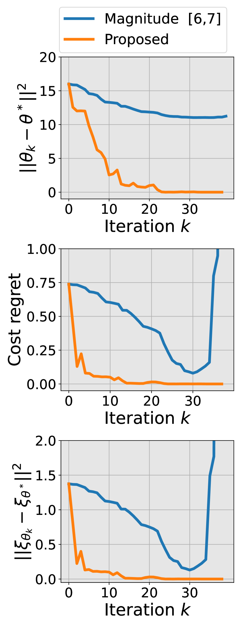
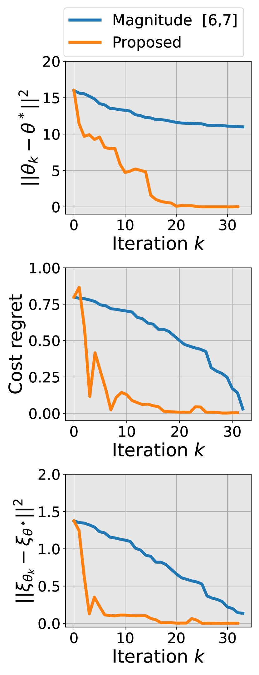
Refer to caption
(a) 𝒂tk=0.00125delimited-∥∥subscript𝒂subscript𝑡𝑘0.00125\lVert\boldsymbol{a}_{t_{k}}\rVert=0.00125
Refer to caption
(b) 𝒂tk=0.001delimited-∥∥subscript𝒂subscript𝑡𝑘0.001\lVert\boldsymbol{a}_{t_{k}}\rVert=0.001
Refer to caption
(c) 𝒂tk=0.0008delimited-∥∥subscript𝒂subscript𝑡𝑘0.0008\lVert\boldsymbol{a}_{t_{k}}\rVert=0.0008
Figure 10: Comparison between the proposed method (in orange lines) and the magnitude-correction methods [6, 7] (in blue lines). Each column corresponds to a different level of correction magnitude, and correction time tksubscript𝑡𝑘t_{k} in different magnitude levels are different random draws. For each magnitude level (each column), the first row shows the weight error versus iteration; the second row is the cost regret versus iteration; and the third row is the trajectory error versus iteration. Detailed analysis is given in the text.

For the magnitude-correction methods [6, 7] (in blue lines) in Fig. 10, comparing different columns, we note that larger magnitude leads to faster convergence. However, as shown by the left and middle panels in the first row, the magnitude-correction method converges to a local weight vector but not 𝜽superscript𝜽\boldsymbol{\theta}^{*}. This is not a surprise, because the magnitude-correction method can only guarantee the convergence of the cost regret, as shown by [6], not necessarily the convergence of the cost function itself. One conjecture to the above results could be that the local weight vector (different from the true 𝜽superscript𝜽\boldsymbol{\theta}^{*}) results in the same robot trajectory and the same optimal cost as 𝜽superscript𝜽\boldsymbol{\theta}^{*} does. This conjecture has been evidenced in the second row and third row in Fig. 10, where the left and middle panels show that the magnitude-correction methods, although having learned a different weight vector, have both the cost regret and trajectory error converging to zero.

Also for the magnitude-correction methods [6, 7] (in blue lines), when 𝒂tk=0.00125delimited-∥∥subscript𝒂subscript𝑡𝑘0.00125\lVert\boldsymbol{a}_{t_{k}}\rVert=0.00125 (first column), we observe that there is a sharp increase of the cost regret and trajectory error near convergence after 30 iterations. This could be because the magnitude-correction methods [6, 7] are not robust against the large magnitude of corrections near the desired trajectory. Specifically, after 303030 iterations near convergence, a relatively larger magnitude, say 𝒂tk=0.00125delimited-∥∥subscript𝒂subscript𝑡𝑘0.00125\lVert\boldsymbol{a}_{t_{k}}\rVert=0.00125, can be an over-correction and thus violating J(𝒖¯0:T𝜽k,𝜽)<J(𝒖0:T𝜽k,𝜽)𝐽subscriptsuperscriptbold-¯𝒖subscript𝜽𝑘:0𝑇superscript𝜽𝐽subscriptsuperscript𝒖subscript𝜽𝑘:0𝑇superscript𝜽J(\boldsymbol{\bar{u}}^{\boldsymbol{\theta}_{k}}_{0:T},\boldsymbol{\theta}^{*})<J(\boldsymbol{{u}}^{\boldsymbol{\theta}_{k}}_{0:T},\boldsymbol{\theta}^{*}). This explanation has been supported by the second column of Fig. 10, where with a smaller magnitude 𝒂tk=0.001delimited-∥∥subscript𝒂subscript𝑡𝑘0.001\lVert\boldsymbol{a}_{t_{k}}\rVert=0.001, there is no such over-correction phenomenon.

Combining all three columns in Fig. 10, one can conclude that for the magnitude-correction methods [6, 7], large correction magnitude, such as 𝒂tk=0.00125delimited-∥∥subscript𝒂subscript𝑡𝑘0.00125\lVert\boldsymbol{a}_{t_{k}}\rVert=0.00125, will have faster convergence, but it can lead to over-corrections, as shown in Fig. 10(a), making the learning process unstable. Smaller correction magnitude, such as 𝒂tk=0.0008delimited-∥∥subscript𝒂subscript𝑡𝑘0.0008\lVert\boldsymbol{a}_{t_{k}}\rVert=0.0008, can avoid the over-correction issue, but it leads to slow convergence, as shown in Fig. 10(c). Notice that the magnitude change from 𝒂tk=0.00125delimited-∥∥subscript𝒂subscript𝑡𝑘0.00125\lVert\boldsymbol{a}_{t_{k}}\rVert=0.00125 (unstable) in Fig. 10(a) to 𝒂tk=0.0008delimited-∥∥subscript𝒂subscript𝑡𝑘0.0008\lVert\boldsymbol{a}_{t_{k}}\rVert=0.0008 (stable) in Fig. 10(c) is very small, which could suggest that the magnitude-correction methods are sensitive to the selection of correction magnitudes. Thus, it could be difficult in practice to provide a valid correction magnitude. We will further show and analyze this in our following user study in Section VI.

In contrast, Fig. 10 has shown that the proposed method consistently learns the true 𝜽superscript𝜽\boldsymbol{\theta}^{*} and achieves a zero cost regret and zero trajectory error regardless of the correction magnitude levels. Also, compared to the magnitude-correction methods [6, 7], the proposed method requires less learning iterations (corrections) for convergence. Since the proposed method only leverages the direction of 𝒂tksubscript𝒂subscript𝑡𝑘\boldsymbol{a}_{t_{k}} regardless of 𝒂tkdelimited-∥∥subscript𝒂subscript𝑡𝑘\lVert\boldsymbol{a}_{t_{k}}\rVert, there is no over-correction issues near convergence. In practice, the choice of directional corrections is more flexible than choosing magnitude corrections, as analyzed in Fig. 3 in Section II. We will continue to show this advantage in the following user study in Section VI.

VI User Study

To show the effectiveness of the proposed method for learning from real human directional corrections, we have developed two human-robot simulation games based on which a user study is conducted. One game is robot arm reaching (Fig. 11) and the other is 6-DoF quadrotor maneuvering (Fig. 12). In each game, a human participant observes the visualization of robot motion, while applying directional corrections through a keyboard. The goal of each game is to teach a robot to learn an objective function, such that it can successfully navigate through an environment without the knowledge about the environment obstacles. We have released the accompanying codes of those two games for the readers to try themselves: https://github.com/wanxinjin/Learning-from-Directional-Corrections.

In what follows next, Sections VI-A and VI-B describe the designs of the two games. Section VI-C provides the details of human participants and the procedure of the user study. The outcomes of the user study are presented in Section VI-D and detailed analysis is given in Section VI-E.

VI-A Robot Arm Reaching Game
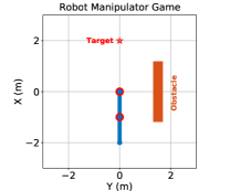
Refer to caption
Figure 11: The robot arm reaching game. A human participant teaches the robot arm to learn a cost function by applying directional corrections via a keyboard (see the instructions in Table I). The goal is to let the robot arm successfully move from the initial pose (the pose in the figure) to reach the target (the star) while avoiding the obstacle. Note that we have no knowledge about the location and size of the obstacle.

VI-A1 Robot Setup

The dynamics of a robot arm and its physical parameters follow Section V-B. The robot initial state is 𝒙0=[π2,0,0,0]𝖳subscript𝒙0superscript𝜋2000𝖳\boldsymbol{x}_{0}{=}[-\frac{\pi}{2},0,0,0]^{\mkern-1.5mu\mathsf{T}}, as in Fig. 11. The parameterized cost function J(𝜽)𝐽𝜽J(\boldsymbol{\theta}) in (2) is

ϕbold-italic-ϕ\displaystyle\boldsymbol{\phi} =[q12,q1,q22,q2,𝒖2]𝖳5,absentsuperscriptsuperscriptsubscript𝑞12subscript𝑞1superscriptsubscript𝑞22subscript𝑞2superscriptdelimited-∥∥𝒖2𝖳superscript5\displaystyle=[q_{1}^{2},\,q_{1},\,{q}_{2}^{2},\,{q}_{2},\,\lVert\boldsymbol{u}\rVert^{2}]^{\mkern-1.5mu\mathsf{T}}\in\mathbb{R}^{5}, (47a)
𝜽𝜽\displaystyle\boldsymbol{\theta} =[θ1,θ2,θ3,θ4,θ5]𝖳5.absentsuperscriptsubscript𝜃1subscript𝜃2subscript𝜃3subscript𝜃4subscript𝜃5𝖳superscript5\displaystyle=[\theta_{1},\theta_{2},\theta_{3},\theta_{4},\theta_{5}]^{\mkern-1.5mu\mathsf{T}}\in\mathbb{R}^{5}. (47b)

Here, 𝜽𝖳ϕsuperscript𝜽𝖳bold-italic-ϕ\boldsymbol{\theta}^{\mkern-1.5mu\mathsf{T}}\boldsymbol{\phi} is a general second-order polynomial. It is worth noting that in practice if prior knowledge about good features is not available, general polynomial features are a good option. The final cost h(𝒙T+1)subscript𝒙𝑇1h(\boldsymbol{x}_{T+1}) in (2) is

h(𝒙T+1)=100((q1π2)2+q22+q˙12+q˙22),subscript𝒙𝑇1100superscriptsubscript𝑞1𝜋22superscriptsubscript𝑞22superscriptsubscript˙𝑞12superscriptsubscript˙𝑞22h(\boldsymbol{x}_{T+1})=100\big{(}(q_{1}-\frac{\pi}{2})^{2}+q_{2}^{2}+\dot{q}_{1}^{2}+\dot{q}_{2}^{2}\big{)}, (48)

as the robot arm aims to finally reach and stop at the target pose: q1target=π2subscriptsuperscript𝑞target1𝜋2{q}^{\text{target}}_{1}=\frac{\pi}{2} and q2target=0subscriptsuperscript𝑞target20{q}^{\text{target}}_{2}=0, marked in Fig. 11. The time horizon of the game is set as T=50𝑇50T=50 (that is, 50Δ=1050Δ1050\Delta=10s). Since we choose the polynomial features (47a), 𝜽𝜽\boldsymbol{\theta} will dictate how the robot reaches the target (i.e., the specific trajectory to the goal). By default, the initial search space 𝛀0subscript𝛀0\boldsymbol{\Omega}_{0} is set

𝛀0={𝜽|θ1,θ3[0,1],θ2,θ4[3,3],θ5[0,0.5]}.subscript𝛀0conditional-set𝜽formulae-sequencesubscript𝜃1subscript𝜃301subscript𝜃2subscript𝜃433subscript𝜃500.5\boldsymbol{\Omega}_{0}{=}\{\boldsymbol{{\theta}}\,|\,\theta_{1},\theta_{3}\in[0,1],\theta_{2},\theta_{4}\in[-3,3],\theta_{5}\in[0,0.5]\}. (49)

Without human corrections, the robot with a random 𝜽0subscript𝜽0\boldsymbol{\theta}_{0} will move and crash into the obstacle in Fig. 11. The goal of the game is to let a human participant teach the robot arm to learn a cost function, such that it can move from the initial condition and reach the target pose while avoiding the obstacle. Note that we have no knowledge about the obstacle.

TABLE I: Keyboard interface for the robot arm game.
Keys Directional correction Interpretation of correction
up 𝒂=[1,0]𝒂10\boldsymbol{a}=[1,0] counter-close-wise torque to Joint 1
down 𝒂=[1,0]𝒂10\boldsymbol{a}=[-1,0] close-wise torque to Joint 1
left 𝒂=[0,1]𝒂01\boldsymbol{a}=[0,1] counter-close-wise torque to Joint 2
right 𝒂=[0,1]𝒂01\boldsymbol{a}=[0,-1] close-wise torque to Joint 2
  • 1

    * When implementing [6, 7], to allow magnitude corrections via the same interface, we additionally detect the key pressing duration δt𝛿𝑡\delta t and interpret the correction magnitude u𝑢u to be proportional to δt𝛿𝑡\delta t with saturation umaxsubscript𝑢u_{\max}; i.e., u=min{βδt,umax}𝑢𝛽𝛿𝑡subscript𝑢u=\min\{\beta\delta t,u_{\max}\} with β=2𝛽2\beta=2 and umax=1subscript𝑢1u_{\max}=1. The magnitude correction using the above interface is 𝒖=u𝒂𝒖𝑢𝒂\boldsymbol{u}=u\boldsymbol{a}. The correction time tksubscript𝑡𝑘t_{k} is the beginning time of the key press.

VI-A2 Interface

In the robot arm game, we use a keyboard as the interface for a human participant to apply directional corrections. We customize (up, down, left, right) keys and associate them with corresponding directional corrections as listed in Table I. During the game, at each learning iteration, a human participant is allowed to press one or multiple keys from (up, down, left, right), and the interface is listening to which key(s) the human player hits and recording the timing of the keystroke(s). The recorded information is translated into the directional correction 𝒂tksubscript𝒂subscript𝑡𝑘\boldsymbol{a}_{t_{k}} as per Table I. For example, at iteration k𝑘k, while the robot is executing the motion trajectory 𝝃𝜽ksubscript𝝃subscript𝜽𝑘\boldsymbol{\xi}_{\boldsymbol{\theta}_{k}}, a human player hits the up and left keys simultaneously at the time step 101010; then the corresponding correction information is translated into 𝒂tk=[1,1]𝖳subscript𝒂subscript𝑡𝑘superscript11𝖳\boldsymbol{a}_{t_{k}}=[1,1]^{\mkern-1.5mu\mathsf{T}} with tk=10subscript𝑡𝑘10t_{k}=10 according to Table I. We obtain averaged 𝒂¯ksubscriptbold-¯𝒂𝑘\boldsymbol{\bar{a}}_{k} from 𝒂tksubscript𝒂subscript𝑡𝑘\boldsymbol{a}_{t_{k}} via (5) and (6b).

VI-B 6-DoF Quadrotor Maneuvering Game
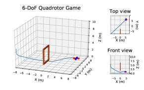
Refer to caption
Figure 12: The 6-DoF quadrotor game. A human participant teaches the quadrotor to learn a cost function by applying directional corrections through a keyboard (see the instruction in Table II). The goal is that the quadrotor can fly from the initial position (in the bottom left), go through a gate (colored in brown), and land on the target (in the upper right). Note that we have no knowledge about the gate.

VI-B1 Robot Setup

The dynamics of a quadrotor is

𝒓˙Isubscript˙𝒓𝐼\displaystyle\dot{\boldsymbol{r}}_{I} =𝒗˙I,absentsubscript˙𝒗𝐼\displaystyle=\dot{\boldsymbol{v}}_{I}, (50a)
m𝒗˙I𝑚subscript˙𝒗𝐼\displaystyle m\dot{\boldsymbol{v}}_{I} =m𝒈I+𝒇I,absent𝑚subscript𝒈𝐼subscript𝒇𝐼\displaystyle=m\boldsymbol{g}_{I}+\boldsymbol{f}_{I}, (50b)
𝒒˙B/Isubscript˙𝒒𝐵𝐼\displaystyle\dot{\boldsymbol{q}}_{B/I} =12Ω(𝝎B)𝒒B/I,absent12Ωsubscript𝝎𝐵subscript𝒒𝐵𝐼\displaystyle=\frac{1}{2}\Omega(\boldsymbol{\omega}_{B}){\boldsymbol{q}}_{B/I}, (50c)
JB𝝎˙Bsubscript𝐽𝐵subscript˙𝝎𝐵\displaystyle J_{B}\dot{\boldsymbol{\omega}}_{B} =𝝉B𝝎B×JB𝝎B.absentsubscript𝝉𝐵subscript𝝎𝐵subscript𝐽𝐵subscript𝝎𝐵\displaystyle=\boldsymbol{\tau}_{B}-\boldsymbol{\omega}_{{B}}\times J_{B}\boldsymbol{\omega}_{B}. (50d)

Here, the subscripts B and I denote the quantities expressed in the quadrotor’s body frame and world frame, respectively; m𝑚m is the mass of the quadrotor; 𝒓I3subscript𝒓𝐼superscript3\boldsymbol{r}_{I}\in\mathbb{R}^{3} and 𝒗I3subscript𝒗𝐼superscript3\boldsymbol{v}_{I}\in\mathbb{R}^{3} are the position and velocity, respectively; JB3×3subscript𝐽𝐵superscript33J_{B}\in\mathbb{R}^{3\times 3} is the moment of inertia; 𝝎B3subscript𝝎𝐵superscript3\boldsymbol{\omega}_{B}\in\mathbb{R}^{3} is the angular velocity; 𝒒B/I4subscript𝒒𝐵𝐼superscript4\boldsymbol{q}_{B/I}\in\mathbb{R}^{4} is the unit quaternion [31] describing the attitude of the quadrotor’s body frame with respect to the world frame; (50c) is the time derivative of the quaternion with Ω(𝝎B)Ωsubscript𝝎𝐵\Omega(\boldsymbol{\omega}_{B}) being the matrix form of 𝝎Bsubscript𝝎𝐵\boldsymbol{\omega}_{B} for quaternion multiplication [31]; 𝝉B3subscript𝝉𝐵superscript3\boldsymbol{\tau}_{B}\in\mathbb{R}^{3} is the torque vector applied to the quadrotor; and 𝒇I3subscript𝒇𝐼superscript3\boldsymbol{f}_{I}\in\mathbb{R}^{3} is the total force vector applied to the center of mass (COM). The total force magnitude 𝒇I=fdelimited-∥∥subscript𝒇𝐼𝑓\lVert\boldsymbol{f}_{I}\rVert={{f}} (along the z-axis of the quadrotor’s body frame) and the torque 𝝉B=[τx,τy,τz]𝖳subscript𝝉𝐵superscriptsubscript𝜏𝑥subscript𝜏𝑦subscript𝜏𝑧𝖳\boldsymbol{\tau}_{B}=[\tau_{x},\tau_{y},\tau_{z}]^{\mkern-1.5mu\mathsf{T}} are generated by four rotor thrusts [T1,T2,T3,T4]𝖳superscriptsubscript𝑇1subscript𝑇2subscript𝑇3subscript𝑇4𝖳[T_{1},T_{2},T_{3},T_{4}]^{\mkern-1.5mu\mathsf{T}} as follows:

[fτxτyτz]=[11110lw/20lw/2lw/20lw/20κκκκ][T1T2T3T4],matrix𝑓subscript𝜏𝑥subscript𝜏𝑦subscript𝜏𝑧matrix11110subscript𝑙w20subscript𝑙w2subscript𝑙w20subscript𝑙w20𝜅𝜅𝜅𝜅matrixsubscript𝑇1subscript𝑇2subscript𝑇3subscript𝑇4\begin{bmatrix}{{f}}\\ \tau_{x}\\ \tau_{y}\\ \tau_{z}\end{bmatrix}=\begin{bmatrix}1&1&1&1\\ 0&-l_{\text{w}}/2&0&l_{\text{w}}/2\\ -l_{\text{w}}/2&0&l_{\text{w}}/2&0\\ \kappa&-\kappa&\kappa&-\kappa\end{bmatrix}\begin{bmatrix}T_{1}\\ T_{2}\\ T_{3}\\ T_{4}\end{bmatrix}, (51)

with lwsubscript𝑙wl_{\text{w}} denoting the wing length of the quadrotor and κ𝜅\kappa a fixed constant, here κ=0.1𝜅0.1\kappa=0.1. In dynamics (50), the gravity constant 𝒈Idelimited-∥∥subscript𝒈𝐼\lVert\boldsymbol{g}_{I}\rVert is set as 101010m/s2 and the other physical parameters are units. We define the state vector of the quadrotor as

𝒙=[𝒓I𝒗I𝒒B/I𝝎B]13,𝒙matrixsubscript𝒓𝐼subscript𝒗𝐼subscript𝒒𝐵𝐼subscript𝝎𝐵superscript13\boldsymbol{x}=\begin{bmatrix}\boldsymbol{r}_{I}&\boldsymbol{v}_{I}&\boldsymbol{q}_{B/I}&\boldsymbol{\omega}_{B}\end{bmatrix}\in\mathbb{R}^{13}, (52)

and the control input vector as

𝒖=[T1T2T3T4]𝖳4.𝒖superscriptmatrixsubscript𝑇1subscript𝑇2subscript𝑇3subscript𝑇4𝖳superscript4\boldsymbol{u}=\begin{bmatrix}T_{1}&T_{2}&T_{3}&T_{4}\end{bmatrix}^{\mkern-1.5mu\mathsf{T}}\in\mathbb{R}^{4}. (53)

We discretize (50) by the Euler method with interval Δ=0.1Δ0.1\Delta=0.1s. To achieve SE𝑆𝐸SE(3) maneuvering, we define the attitude error between the quadrotor attitude 𝒒𝒒\boldsymbol{q} and target 𝒒targetsuperscript𝒒target\boldsymbol{q}^{\text{target}} as [32]

e(𝒒,𝒒target)=12trace(IR𝖳(𝒒target)R(𝒒)),𝑒𝒒subscript𝒒target12trace𝐼superscript𝑅𝖳superscript𝒒target𝑅𝒒e(\boldsymbol{q},\boldsymbol{q}_{\text{target}})=\small{\frac{1}{2}}\text{trace}(I-R^{\mkern-1.5mu\mathsf{T}}(\boldsymbol{q}^{\text{target}})R(\boldsymbol{q})), (54)

where R(𝒒)3×3𝑅𝒒superscript33R(\boldsymbol{q})\in\mathbb{R}^{3\times 3} is the rotation matrix corresponding to 𝒒𝒒\boldsymbol{q}.

In the cost function (2), we set the final cost term as

h(𝒙T+1)=subscript𝒙𝑇1absent\displaystyle h({\boldsymbol{x}_{T+1}})=\, 𝒓I𝒓Itarget2+10𝒗I2+superscriptdelimited-∥∥subscript𝒓𝐼superscriptsubscript𝒓𝐼target2limit-from10superscriptdelimited-∥∥subscript𝒗𝐼2\displaystyle\lVert\boldsymbol{r}_{I}-\boldsymbol{r}_{I}^{\text{target}}\rVert^{2}+10\lVert\boldsymbol{v}_{I}\rVert^{2}+
100e(𝒒B/I,𝒒B/Itarget)+10𝒘B2,100𝑒subscript𝒒𝐵𝐼superscriptsubscript𝒒𝐵𝐼target10superscriptdelimited-∥∥subscript𝒘𝐵2\displaystyle 100e(\boldsymbol{q}_{B/I},\boldsymbol{q}_{B/I}^{\text{target}})+10\lVert\boldsymbol{w}_{B}\rVert^{2}, (55)

because the quadrotor aims to finally land on a target position 𝒓Itargetsuperscriptsubscript𝒓𝐼target\boldsymbol{r}_{I}^{\text{target}} with a target attitude 𝒒B/Itargetsuperscriptsubscript𝒒𝐵𝐼target\boldsymbol{q}_{B/I}^{\text{target}}. Here, 𝒓I=[rx,ry,rz]𝖳subscript𝒓𝐼superscriptsubscript𝑟𝑥subscript𝑟𝑦subscript𝑟𝑧𝖳\boldsymbol{r}_{I}=[r_{x},r_{y},r_{z}]^{\mkern-1.5mu\mathsf{T}} is the position of the quadrotor expressed in the world frame. We set the weight-feature cost term as

ϕbold-italic-ϕ\displaystyle\boldsymbol{\phi} =[rx2rxry2ryrz2rz𝒖2]𝖳7,absentsuperscriptmatrixsuperscriptsubscript𝑟𝑥2subscript𝑟𝑥superscriptsubscript𝑟𝑦2subscript𝑟𝑦superscriptsubscript𝑟𝑧2subscript𝑟𝑧superscriptdelimited-∥∥𝒖2𝖳superscript7\displaystyle=\begin{bmatrix}r_{x}^{2}&r_{x}&r_{y}^{2}&r_{y}&r_{z}^{2}&r_{z}&\lVert\boldsymbol{u}\rVert^{2}\end{bmatrix}^{\mkern-1.5mu\mathsf{T}}\in\mathbb{R}^{7}, (56a)
𝜽𝜽\displaystyle\boldsymbol{\theta} =[θ1θ2θ3θ4θ5θ6θ7]𝖳7.absentsuperscriptmatrixsubscript𝜃1subscript𝜃2subscript𝜃3subscript𝜃4subscript𝜃5subscript𝜃6subscript𝜃7𝖳superscript7\displaystyle=\begin{bmatrix}\theta_{1}&\theta_{2}&\theta_{3}&\theta_{4}&\theta_{5}&\theta_{6}&\theta_{7}\end{bmatrix}^{\mkern-1.5mu\mathsf{T}}\in\mathbb{R}^{7}. (56b)

Here, feature vector ϕbold-italic-ϕ\boldsymbol{\phi} consists of general polynomial features and 𝜽𝜽\boldsymbol{\theta} will determine the specific trajectory of the quadrotor to the target. By default, the initial weight search space is

𝛀0={𝜽|θ1,θ3,θ5[0,1],θ2,θ4,θ6[8,8],θ7[0,0.5]}.subscript𝛀0conditional-set𝜽formulae-sequencesubscript𝜃1subscript𝜃3subscript𝜃501subscript𝜃2subscript𝜃4subscript𝜃688subscript𝜃700.5\boldsymbol{\Omega}_{0}{=}\{\boldsymbol{{\theta}}\,|\,\theta_{1},\theta_{3},\theta_{5}\in[0,1],\\ \theta_{2},\theta_{4},\theta_{6}\in[-8,8],\theta_{7}\in[0,0.5]\}. (57)

As in Fig. 12, the goal of this quadrotor game is to let a human participant teach the quadrotor to learn a cost function, such that the quadrotor can successfully fly from the initial position 𝒓I(0)=[8,8,5]𝖳subscript𝒓𝐼0superscript885𝖳\boldsymbol{r}_{I}(0)=[-8,-8,5]^{\mkern-1.5mu\mathsf{T}} (in the bottom left), go through a gate (in brown color), and finally land on a target position 𝒓Itarget=[8,8,0]𝖳superscriptsubscript𝒓𝐼targetsuperscript880𝖳\boldsymbol{r}_{I}^{\text{target}}=[8,8,0]^{\mkern-1.5mu\mathsf{T}} (in the upper right) with the target attitude 𝒒B/Itarget=[1,0,0,0]𝖳superscriptsubscript𝒒𝐵𝐼targetsuperscript1000𝖳\boldsymbol{q}_{B/I}^{\text{target}}=[1,0,0,0]^{\mkern-1.5mu\mathsf{T}}. The initial attitude of the quadrotor is 𝒒B/I(0)=[1,0,0,0]𝖳subscript𝒒𝐵𝐼0superscript1000𝖳\boldsymbol{q}_{B/I}(0)=[1,0,0,0]^{\mkern-1.5mu\mathsf{T}} and initial velocities zeros. The time horizon for this game is T=50𝑇50T=50, that is, TΔ=5𝑇Δ5T\Delta=5s. Note that we have no knowledge about the gate.

TABLE II: Keyboard interface for 6-DoF quadrotor game.
Keys Directional correction Interpretation of correction
‘up’
T1=1,T2=1,formulae-sequencesubscript𝑇11subscript𝑇21T_{1}{=}1,T_{2}{=}1,
T3=1,T4=1formulae-sequencesubscript𝑇31subscript𝑇41T_{3}{=}1,T_{4}{=}1
Upward force applied at COM
‘down’
T1=1,T2=1,formulae-sequencesubscript𝑇11subscript𝑇21T_{1}{=}{-}1,T_{2}{=}{-}1,
T3=1,T4=1formulae-sequencesubscript𝑇31subscript𝑇41T_{3}{=}{-}1,T_{4}{=}{-}1
Downward force applied at COM
‘w’
T1=0,T2=1formulae-sequencesubscript𝑇10subscript𝑇21T_{1}{=}0,T_{2}{=}1
T3=0,T4=1formulae-sequencesubscript𝑇30subscript𝑇41T_{3}{=}0,T_{4}{=}{-}1
Negative torque along body-axis x
‘s’
T1=0,T2=1formulae-sequencesubscript𝑇10subscript𝑇21T_{1}{=}0,T_{2}{=}{-}1
T3=0,T4=1formulae-sequencesubscript𝑇30subscript𝑇41T_{3}{=}0,T_{4}{=}1
Positive torque along body-axis x
‘a’
T1=1,T2=0formulae-sequencesubscript𝑇11subscript𝑇20T_{1}{=}1,T_{2}{=}0
T3=1,T4=0formulae-sequencesubscript𝑇31subscript𝑇40T_{3}{=}{-}1,T_{4}{=}0
Negative torque along body-axis y
‘d’
T1=1,T2=0formulae-sequencesubscript𝑇11subscript𝑇20T_{1}{=}{-}1,T_{2}{=}0
T3=1,T4=0formulae-sequencesubscript𝑇31subscript𝑇40T_{3}{=}1,T_{4}{=}0
Positive torque along body-axis y
  • 1

    * When implementing [6, 7], to allow magnitude corrections via the same interface, we additionally detect key pressing duration δt𝛿𝑡\delta t and interpret the correction magnitude u𝑢u to be u=min{βδt,umax}𝑢𝛽𝛿𝑡subscript𝑢u=\min\{\beta\delta t,u_{\max}\} with β=2𝛽2\beta{=}2 and umax=1subscript𝑢1u_{\max}{=}1 in our implementation. Thus, the magnitude correction using the above interface is 𝒖=u[T1,T2,T3,T4]𝖳𝒖𝑢superscriptsubscript𝑇1subscript𝑇2subscript𝑇3subscript𝑇4𝖳\boldsymbol{u}=u[T_{1},T_{2},T_{3},T_{4}]^{\mkern-1.5mu\mathsf{T}}. The correction time tksubscript𝑡𝑘t_{k} is the beginning time of the key press.

VI-B2 Interface

The keyboard interface for applying directional corrections is in Table II. Specifically, we customize the (‘up’, ‘down’, ‘w’, ‘s’, ‘a’, ‘d’) keys and map them to specific directional correction signals. During a learning iteration, a human participant is allowed to press one or multiple keys in Table II. The interface listens to the keystrokes and translates the keystrokes into the directional corrections based on Table II. The time step at which a key is hit is the correction time tksubscript𝑡𝑘t_{k}. For example, if a human participant presses ‘s’ key at time step 555; then, the directional correction will be 𝒂tk=[0,1,0,1]𝖳subscript𝒂subscript𝑡𝑘superscript0101𝖳\boldsymbol{a}_{t_{k}}=[0,-1,0,1]^{\mkern-1.5mu\mathsf{T}} with tk=5subscript𝑡𝑘5t_{k}=5. Based on (5) and (6b), we obtain 𝒂¯ksubscriptbold-¯𝒂𝑘\boldsymbol{\bar{a}}_{k} from 𝒂tksubscript𝒂subscript𝑡𝑘\boldsymbol{a}_{t_{k}}.

VI-C Participants and Procedure

A total of 17 volunteers from Purdue College of Engineering have participated in our user study. Among these 17 participants, 1 was female and 16 male, with ages from 20 to 37 years old (25.812±3.936plus-or-minus25.8123.93625.812\pm 3.936). 5 of those 17 participants had no robotics or related background, and all participants were novices to the two games. This user study had been reviewed and approved by the Institutional Review Board (IRB) of Purdue University, and all participants had signed the consent forms.

Each participant was instructed to play the above two games. In each game, a participant played 5 successive rounds with the proposed method and 5 successive rounds with the magnitude-correction method [6, 7]. A game round is defined as a complete run of a learning method until the success or failure of the round. A failure of a game round is identified if the robot fails to accomplish the task after the total number of human corrections has exceeded the maximum correction count. In our user study, the maximum correction count is 20 for the robot arm game and 15 for the quadrotor game. We set the maximum correction count because the participants are expected to try their best to teach the robot with as few corrections as possible.

We used a within-subjects design: the order of the two games (i.e., which game goes first) and learning methods used (i.e., which method is used first) were counterbalanced across all participants in our user study. Also, the participants were not informed which methods were being used for the current game. Before starting a game, each participant was instructed how to play the game and was given one hands-on game round to get familiar with the interface before the experiment recording starts. After the games, each participant was asked to finish a post-game survey about her/his opinions of the game experience (which will be reported in Section VI-E4).
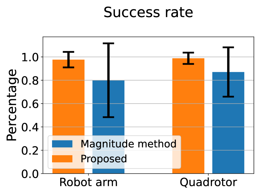
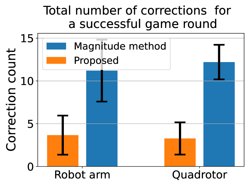
Refer to caption
(a) Success rate
Refer to caption
(b) Total correction count in a success game
Refer to caption
(c) Early wasted rounds
Figure 13: The outcomes of all 17 participants for playing different robot games (robot-arm or quadrotor) using different learning methods (the proposed method and magnitude-correction method [6, 7]). (a) shows the success rate, i.e., the ratio of successful game rounds over total 5 rounds attempted; (b) shows the total number of human corrections needed for one successful game round; and (c) shows the number of the early wasted (failed) game rounds before a participant constantly play successfully. The bars denote the mean values over all participants, and the top line segments are the standard deviations. Analysis based on statistical tests (with significance level α=0.05𝛼0.05\alpha=0.05) is in Section VI-E. One illustrative round for the robot arm game from one participant is in Fig. 14 and Table III, and one illustrative quadrotor game round from a participant is in Fig. 15 and Table IV.

VI-D Outcome Measurements

For each game (robot arm or quadrotor) with each learning method (the proposed method or magnitude-correction method [6, 7]), we measure the following outcomes for one participant in his/her 5-successive game rounds.

  • Success rate. This is the ratio of successful game rounds over all rounds attempted (which is 5 here). This outcome indicates the efficacy of a learning method.

  • Total number of corrections for a successful game round. This measures how many human corrections are needed for a successful game round. This measure can show the efficiency/effortlessness of a learning method—fewer corrections mean less human effort in teaching a robot.

  • Early wasted rounds. This is to measure how many early rounds of a game are wasted (failed) before a participant begins to constantly play successful game rounds. This can show the accessibility of a learning method—fewer early wasted rounds indicate a more accessible experience for a participant to successfully teach a robot.

The outcomes of all participants are organized according to the method type (the proposed method and magnitude-correction method [6, 7]) and the game type (robot-arm and quadrotor). We report all outcomes in Fig. 13 and provide a detailed analysis of the results based on statistical tests.

VI-E Results and Analysis

The statistics of three outcomes over all 17 participants are shown in Fig. 13. Each outcome is presented with respect to each learning method (the proposed method or magnitude-correction method [6, 7]) on each game (robot arm or quadrotor). All three outcomes here are averaged over all participants with the error bar denoting the standard deviation over all participants. We have the following analysis of the results based on statistical tests with significance level α=0.05𝛼0.05\alpha=0.05,

Refer to caption
(a) Iteration k=1𝑘1k=1
Refer to caption
(b) Iteration k=2𝑘2k=2
Refer to caption
(c) Iteration k=3𝑘3k=3
Refer to caption
(d) Iteration k=4𝑘4k=4
Figure 14: One illustrative round for the robot arm game from one participant. At each iteration k𝑘k, the robot weight vector guess 𝜽ksubscript𝜽𝑘\boldsymbol{{\theta}}_{k} and the participant directional correction 𝒂tksubscript𝒂subscript𝑡𝑘\boldsymbol{a}_{t_{k}} are reported in Table III.
TABLE III: An illustrative round for the robot arm game from one participant.
Iteration k𝑘k Current weight vector guess 𝜽ksubscript𝜽𝑘\boldsymbol{\theta}_{k} A participant’s directional correction 𝒂tksubscript𝒂subscript𝑡𝑘\boldsymbol{a}_{t_{k}} and correction time tksubscript𝑡𝑘{t_{k}}
k=1𝑘1k=1 𝜽k=[0.50, 0.00, 0.50,0.00, 0.25]𝖳subscript𝜽𝑘superscript0.500.000.500.000.25𝖳\boldsymbol{\theta}_{k}=[0.50,\,0.00,\,0.50,-0.00,\,0.25]^{\mkern-1.5mu\mathsf{T}} 𝒂tk=[0,1]subscript𝒂subscript𝑡𝑘01\boldsymbol{a}_{t_{k}}=[0,1] (i.e., left key pressed)  and  tk=11subscript𝑡𝑘11{t_{k}}=11
k=2𝑘2k=2 𝜽k=[0.50, 0.00, 0.50,1.50, 0.25]𝖳subscript𝜽𝑘superscript0.500.000.501.500.25𝖳\boldsymbol{\theta}_{k}=[0.50,\,0.00,\,0.50,-1.50,\,0.25]^{\mkern-1.5mu\mathsf{T}} 𝒂tk=[0,1]subscript𝒂subscript𝑡𝑘01\boldsymbol{a}_{t_{k}}=[0,1] (i.e., left key pressed)  and  tk=16subscript𝑡𝑘16{t_{k}}=16
k=3𝑘3k=3 𝜽k=[0.50, 0.00, 0.34,2.03, 0.25]𝖳subscript𝜽𝑘superscript0.500.000.342.030.25𝖳\boldsymbol{\theta}_{k}=[0.50,\,0.00,\,0.34,-2.03,\,0.25]^{\mkern-1.5mu\mathsf{T}} 𝒂tk=[1,0]subscript𝒂subscript𝑡𝑘10\boldsymbol{a}_{t_{k}}=[-1,0] (i.e., down key pressed)  and tk=34subscript𝑡𝑘34{t_{k}}=34
k=4𝑘4k=4 𝜽k=[0.50, 1.48, 0.36,2.00, 0.25]𝖳subscript𝜽𝑘superscript0.501.480.362.000.25𝖳\boldsymbol{\theta}_{k}=[0.50,\,1.48,\,0.36,-2.00,\,0.25]^{\mkern-1.5mu\mathsf{T}} Game success!
Refer to caption
(a) Iteration k=2𝑘2k=2
Refer to caption
(b) Iteration k=3𝑘3k=3
Refer to caption
(c) Iteration k=4𝑘4k=4
Refer to caption
(d) Iteration k=5𝑘5k=5
Figure 15: One illustrative round for the quadrotor game from one participant. At each iteration k𝑘k, the quadrotor weight vector guess 𝜽ksubscript𝜽𝑘\boldsymbol{{\theta}}_{k} and the participant directional correction 𝒂tksubscript𝒂subscript𝑡𝑘\boldsymbol{a}_{t_{k}} are in Table IV. Iteration k=1𝑘1k=1 is shown in Fig. 12.
TABLE IV: An illustrative round for the quadrotor game from one participant (Iteration k=1𝑘1k=1 is shown in Fig. 12).
Iteration k𝑘k Current weight vector guess 𝜽ksubscript𝜽𝑘\boldsymbol{\theta}_{k} A participant’s directional corrections 𝒂tksubscript𝒂subscript𝑡𝑘\boldsymbol{a}_{t_{k}} and correction time tksubscript𝑡𝑘{t_{k}}
k=1𝑘1k=1 𝜽k=[0.50, 0.00, 0.50,0.00, 0.50,0.00, 0.25]𝖳subscript𝜽𝑘superscript0.500.000.500.000.500.000.25𝖳\boldsymbol{\theta}_{k}=[0.50,\,0.00,\,0.50,-0.00,\,0.50,\,-0.00,\,0.25]^{\mkern-1.5mu\mathsf{T}}
𝒂tk=[1,1,1,1]subscript𝒂subscript𝑡𝑘1111\boldsymbol{a}_{t_{k}}=[1,1,1,1] (i.e., up key pressed)  and     tk=8subscript𝑡𝑘8{t_{k}}=8
𝒂tk=[1,1,1,1]subscript𝒂subscript𝑡𝑘1111\boldsymbol{a}_{t_{k}}=[1,1,1,1] (i.e., up key pressed)  and  tk=20subscript𝑡𝑘20{t_{k}}=20
k=2𝑘2k=2 𝜽k=[0.50,0.00, 0.50,0.00, 0.50,3.99, 0.25]𝖳subscript𝜽𝑘superscript0.500.000.500.000.503.990.25𝖳\boldsymbol{\theta}_{k}=[0.50,\,-0.00,\,0.50,-0.00,\,0.50,\,-3.99,\,0.25]^{\mkern-1.5mu\mathsf{T}} 𝒂tk=[1,1,1,1]subscript𝒂subscript𝑡𝑘1111\boldsymbol{a}_{t_{k}}=[-1,-1,-1,-1] (i.e., down key pressed)  and  tk=14subscript𝑡𝑘14{t_{k}}=14
k=3𝑘3k=3 𝜽k=[0.50,1.70, 0.50,1.70, 0.52,1.89, 0.25]𝖳subscript𝜽𝑘superscript0.501.700.501.700.521.890.25𝖳\boldsymbol{\theta}_{k}=[0.50,\,-1.70,\,0.50,-1.70,\,0.52,\,-1.89,\,0.25]^{\mkern-1.5mu\mathsf{T}} 𝒂tk=[0,1,0,1]subscript𝒂subscript𝑡𝑘0101\boldsymbol{a}_{t_{k}}=[0,-1,0,1] (i.e., ’s’ key pressed)  and tk=13subscript𝑡𝑘13{t_{k}}=13
k=4𝑘4k=4 𝜽k=[0.50,2.76, 0.50,2.45, 0.60,2.22, 0.25]𝖳subscript𝜽𝑘superscript0.502.760.502.450.602.220.25𝖳\boldsymbol{\theta}_{k}=[0.50,\,-2.76,\,0.50,-2.45,\,0.60,\,-2.22,\,0.25]^{\mkern-1.5mu\mathsf{T}} 𝒂tk=[0,1,0,1]subscript𝒂subscript𝑡𝑘0101\boldsymbol{a}_{t_{k}}=[0,-1,0,1] (i.e., ’s’ key pressed)  and tk=19subscript𝑡𝑘19{t_{k}}=19
k=5𝑘5k=5 𝜽k=[0.50,3.11, 0.50, 4.89, 0.652.67, 0.25]𝖳subscript𝜽𝑘superscript0.503.110.504.890.652.670.25𝖳\boldsymbol{\theta}_{k}=[0.50,\,-3.11,\,0.50,\,4.89,\,0.65\,-2.67,\,0.25]^{\mkern-1.5mu\mathsf{T}} Game success!

VI-E1 Success Rate

In Fig. 13(a), for the robot arm game, the proposed method obtains a success rate of 97.65%±6.64%plus-or-minuspercent97.65percent6.6497.65\%\pm 6.64\% compared to the magnitude-correction method [6, 7]’s 80.00%±31.62%plus-or-minuspercent80.00percent31.6280.00\%\pm 31.62\%. The proposed method yields a significantly higher success rate than the magnitude-correction method with t𝑡t-score t=2.25𝑡2.25t=2.25 and p𝑝p-value p=0.031<α𝑝0.031𝛼p=0.031<\alpha. For the quadrotor game in Fig. 13(a), the proposed method attains 94%±12.8%plus-or-minuspercent94percent12.894\%\pm 12.8\% versus the magnitude-correction method’s 82%±20.9%plus-or-minuspercent82percent20.982\%\pm 20.9\%. It also shows a significantly higher success rate than the magnitude-correction method [6, 7], with t𝑡t-score t=2.24𝑡2.24t=2.24 and p𝑝p-value p=0.032α𝑝0.032𝛼p=0.032\leq\alpha.

We provide the following comments for the above results. Recall that the magnitude-correction method [6, 7] assumes J(𝒖0:T𝜽k+𝒂¯k,𝜽)<J(𝒖0:T𝜽k,𝜽)𝐽superscriptsubscript𝒖:0𝑇subscript𝜽𝑘subscriptbold-¯𝒂𝑘superscript𝜽𝐽superscriptsubscript𝒖:0𝑇subscript𝜽𝑘superscript𝜽\small J(\boldsymbol{u}_{0:T}^{\boldsymbol{{\theta}}_{k}}+\boldsymbol{\bar{a}}_{k},\boldsymbol{\theta}^{*}){<}J(\boldsymbol{u}_{0:T}^{\boldsymbol{{\theta}}_{k}},\boldsymbol{\theta}^{*}), while the our method assumes J(𝒖0:T𝜽k,𝜽),𝒂¯k>0𝐽superscriptsubscript𝒖:0𝑇subscript𝜽𝑘superscript𝜽subscriptbold-¯𝒂𝑘0\langle-\nabla J(\boldsymbol{u}_{0:T}^{\boldsymbol{\theta}_{k}},\boldsymbol{\theta}^{*}),\boldsymbol{\bar{a}}_{k}\rangle{>}0, regardless of magnitude 𝒂¯𝒌delimited-∥∥subscriptbold-¯𝒂𝒌\lVert\boldsymbol{\bar{a}_{k}}\rVert. As shown in Fig. 3, the allowable region of directional corrections is much larger than that of magnitude corrections. Since all participants are novices to both games, giving valid magnitude correction could be difficult for them. By contrast, novice participants are more likely to give valid directional corrections. This leads to higher success rate and lower variance for the proposed method than the magnitude-correction method.

The difficulty of giving valid magnitude corrections can also be seen from the number of early wasted/failed rounds in Fig. 13(c). For the magnitude method, before a participant masters a game, 0.82±1.42plus-or-minus0.821.420.82\pm 1.42 early game rounds are wasted/failed for the robot arm game, and 0.24±0.56plus-or-minus0.240.560.24\pm 0.56 early rounds are failed for the quadrotor game. In contrast, the proposed method has 0±0plus-or-minus000\pm 0 early wasted rounds in both games. This means that a novice participant needs more practice to master the skill of giving valid magnitude corrections.

VI-E2 Total Number of Corrections for Successful Game

In Fig. 13(b), for a successful robot arm game, the proposed method needs a total of 3.66±2.29plus-or-minus3.662.293.66\pm 2.29 corrections, while the magnitude-correction method [6, 7] requires 11.21±3.62plus-or-minus11.213.6211.21\pm 3.62 corrections. Thus, the proposed method requires significantly fewer corrections than the magnitude-correction method, with t𝑡t-score t=7.27𝑡7.27t=7.27 and p𝑝p-value p=2.94×10⁸α𝑝2.94superscript108𝛼p=2.94\times 10^{-8}\leq\alpha. In the quadrotor game, the proposed method takes a total of 3.27±1.88plus-or-minus3.271.883.27\pm 1.88 corrections for a successful round, while the magnitude-correction method needs 12.20±2.02plus-or-minus12.202.0212.20\pm 2.02 corrections. This again shows that the proposed method is significantly more efficient (fewer corrections) than the magnitude-correction method, with t𝑡t-score t=13.32𝑡13.32t=13.32 and p𝑝p-value p=1.35×10¹⁴<α𝑝1.35superscript1014𝛼p=1.35\times 10^{-14}<\alpha.

We have the following interpretations for the above results. Recall that the assumption for a valid magnitude correction 𝒂¯ksubscriptbold-¯𝒂𝑘\boldsymbol{\bar{a}}_{k} is J(𝒖0:T𝜽k+𝒂¯k,𝜽)<J(𝒖0:T𝜽k,𝜽)𝐽superscriptsubscript𝒖:0𝑇subscript𝜽𝑘subscriptbold-¯𝒂𝑘superscript𝜽𝐽superscriptsubscript𝒖:0𝑇subscript𝜽𝑘superscript𝜽J(\boldsymbol{u}_{0:T}^{\boldsymbol{{\theta}}_{k}}+\boldsymbol{\bar{a}}_{k},\boldsymbol{\theta}^{*}){<}J(\boldsymbol{u}_{0:T}^{\boldsymbol{{\theta}}_{k}},\boldsymbol{\theta}^{*}). Since all participants are novice to the games, the magnitude corrections made by a participant were not always valid in a game round; in other words, some magnitude corrections can be over-correction. Because of those invalid corrections, the magnitude-correction method takes longer (more corrections) to succeed. In contrast, the proposed method only leverages directional corrections, which are more likely to satisfy J(𝒖0:T𝜽k,𝜽),𝒂¯k>0𝐽superscriptsubscript𝒖:0𝑇subscript𝜽𝑘superscript𝜽subscriptbold-¯𝒂𝑘0\langle-\nabla J(\boldsymbol{u}_{0:T}^{\boldsymbol{\theta}_{k}},\boldsymbol{\theta}^{*}),\boldsymbol{\bar{a}}_{k}\rangle{>}0; it requires fewer human corrections (effort).

Since the total number of corrections for a successful game indicates how much effort a participant needs to successfully teach a robot. Thus, the above results in Fig. 13(b) show that the proposed method is significantly more effortless than the magnitude-correction method [6, 7].

VI-E3 Early Wasted Rounds

In Fig. 13(c), in the robot arm game (5 rounds in total), the early wasted (failed) rounds is 0±0plus-or-minus000\pm 0 for the proposed method and 0.82±1.42plus-or-minus0.821.420.82\pm 1.42 for the magnitude-correction method [6, 7]; thus, the proposed method requires significantly fewer rounds of practice (thus is more accessible) than the magnitude-correction method, with t𝑡t-score t=2.38𝑡2.38t=2.38 and p𝑝p-value p=0.02<α𝑝0.02𝛼p=0.02<\alpha. For the quadrotor game (5 rounds in total), a participant wasted 0±0plus-or-minus000\pm 0 early rounds using the proposed method, while 0.24±0.56plus-or-minus0.240.560.24\pm 0.56 early rounds using the magnitude-correction method. The early wasted rounds of the proposed method are not significantly lower than that of the magnitude-correction method, with t𝑡t-score t=1.73𝑡1.73t=1.73 and p𝑝p-value p=0.09>α𝑝0.09𝛼p=0.09>\alpha.

We have the following explanations for the above results. For the magnitude-correction method, since not all magnitude corrections are valid, a participant needs more early trials to realize the effects of correction magnitude on the robot motion and how to apply valid magnitude. Instead, for the proposed method, a participant only gives directional commands, which can be more intuitive, as shown in Fig. 14 and Fig. 15. Fig. 13(c) shows that the proposed method is potentially more accessible than the magnitude-correction method [6, 7]

VI-E4 Other Observations and Subjective Survey

We also observe that the number of the directional corrections in the user study is generally smaller than that in the simulation cases in Section V. This is because the convergence of the robot motion trajectory (to the desired motion in the human’s perspective) is empirically faster than the convergence of the cost function weight vector (to the true 𝜽superscript𝜽\boldsymbol{\theta}^{*}). This has been shown in Fig. 10, where the convergence of 𝜽k𝜽2superscriptdelimited-∥∥subscript𝜽𝑘superscript𝜽2\lVert\boldsymbol{\theta}_{k}-\boldsymbol{\theta}^{*}\rVert^{2} requires around 20 iterations, while the convergence of 𝝃𝜽k𝝃𝜽2superscriptdelimited-∥∥subscript𝝃subscript𝜽𝑘subscript𝝃superscript𝜽2\lVert\boldsymbol{\xi}_{\boldsymbol{\theta}_{k}}-\boldsymbol{\xi}_{\boldsymbol{\theta}^{*}}\rVert^{2} requires only 10 iterations. Since a game is deemed successful as long as the robot motion can successfully navigate through the environment, thus a participant usually takes fewer corrections. We also find that there is no unique solution for the choice of directional corrections and that different participants applied different corrections to manage the games.

We have also performed a post-game survey about how participants perceived the two learning methods. 10 out of 17 participants said that they felt the robot with the proposed method is much ‘smarter’ than the robot with the magnitude-correction method [6, 7]. Those opinions are also consistent with the results in Fig. 13, as we have analyzed above.

VI-E5 Summary

In summary of all statistical analysis above, we conclude that compared to the state-of-the-art magnitude-correction method [6, 7], the proposed method is

  • significantly more effective (p<0.033𝑝0.033p<0.033) — it attains higher success rate for teaching robots,

  • significantly more efficient (p<107𝑝superscript107p<10^{-7}) — fewer human corrections are needed for successful robot learning,

  • potentially more accessible (p0.09𝑝0.09p\leq 0.09) for human users — a novice human user takes fewer trials before constantly providing successful corrections to a robot.

The post-game survey reports that a majority of the user-study participants indicated that a robot with the proposed method is much ‘smarter’ than with the magnitude-correction method.

VII Real-world Experiment

In this section, we test the proposed method in a real-world experiment using a Parrot Mambo quadrotor.
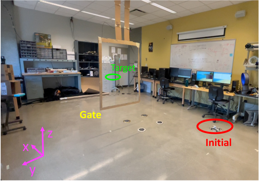
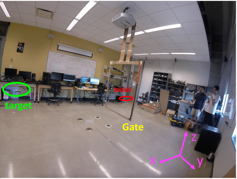
Refer to caption
(a) Main camera view
Refer to caption
(b) Back camera view
Figure 16: The setup of the real-world experiment. A human user teaches the quadrotor to fly from an initial position (red circle), go through the gate (with yellow label), and finally, land on a target position (green circle). Without human corrections, the quadrotor is initialized with a random cost function and fails to accomplish the task. Note that we have no knowledge about the gate.
Refer to caption
(a) Iteration k=1𝑘1k=1
Refer to caption
(b) Iteration k=2𝑘2k=2
Refer to caption
(c) Iteration k=3𝑘3k=3
Refer to caption
(d) Iteration k=4𝑘4k=4
Figure 17: Results of a real-world quadrotor learning from human directional corrections. Here, the quadrotor trajectory is marked in red lines. The initial position (red circle) and target position (green circle) are also marked. In (a), during the quadrotor flying, the human user applied a torque correction in the opposite of the x-axis, shown by the green arrow. In (b), during the quadrotor flying, the human user applied a upward thrust correction (in green arrow) in z-axis. In (c), the quadrotor detected a potential collision with the left pillar of the gate and thus triggered an emergence stop. But before the emergence stop, the human user had already applied a positive x-axis (in green arrow) torque to correct the quadrotor. In (d), the quadrotor successfully learned a cost function to fly from the initial position, go through the gate, and finally reach the target position.

VII-A Experiment Setup and Procedure

Our real-world experiment is a Parrot Mambo quadrotor task shown in Fig. 16. The goal of the experiment is to let a human user teach the quadrotor to accomplish the following task: starting from the initial position (red circle), flying through the gate (labeled in yellow), and landing on the target position (green circle). Without human correction, the quadrotor with a random initial cost function fails to accomplish the task. The procedure of learning from human directional corrections is as follows:

  • First, perform the quadrotor motion planning in a remote computer by solving a trajectory optimization with the current cost function;

  • Second, the quadrotor executes the plan (tracking control), at the same time a human user watches the quadrotor’s motion and applies directional corrections via the keyboard of the remote computer.

  • Third, update the quadrotor’s cost function in the remote computer according to Algorithm 1; then repeat the above steps until the success of the task.

In the above procedure, the interface for a human user to apply directional corrections is still a keyboard, following Table II. The communication frequency between the quadrotor and the remote computer is around 10Hz. Note that because the cost function in some learning iterations may lead the quadrotor to collide with the gate during execution, we have included a collision stop mechanism: if the quadrotor detects that it is too close to the gate, an emergence stop is triggered. In the iteration where an emergence stop is triggered, human corrections, if applied before an emergence stop, can still count for updating the cost function for the next iteration. We will discuss the damage protection of robot learning in details in Appendix B-C.

We have invited a human user (not the co-authors themselves), who is a novice to our work, to perform the above experiment. The human user first had a successful warm-up training in our previous quadrotor game in order to get familiar with the interface (Table II), and then successfully conducted this real-world quadrotor experiment in just one run.

VII-B Results and Analysis

The results in all learning iterations are in Fig. 17. At each iteration, the quadrotor’s trajectory is highlighted in the red lines, and the human directional corrections are labeled in the green arrows. The initial and target positions are also marked. We provide the following analysis for the results in Fig. 17.

In the first iteration in Fig. 17(a), since the quadrotor was initialized with a random cost function, the planned and executed trajectory (labeled in the red line) are off the gate—the quadrotor missed the gate and flew from its right side. Thus, when observing the quadrotor’s motion, the human user applied a directional toque to correct the quadrotor, which is in the direction of the negative x-axis, as shown by the green arrow in Fig. 17(a). After receiving the correction, the quadrotor updated its cost function and planned a new trajectory for the next iteration in Fig. 17(b). In the second iteration in Fig. 17(b), while the quadrotor was executing the new motion, the human user observed that its motion was too below the gate and thus applied a directional force in the positive z-axis. Using this directional correction, the quadrotor updated its cost function for the third iteration in Fig. 17(c).

In the third iteration in Fig. 17(c), while executing the planned motion, the quadrotor detected a potential collision with the left pillar of the gate and thus immediately triggered an emergence stop. However, because humans are able to predict the potential collision, the human user had already applied a directional torque in the positive x-axis (the green arrow) before the emergence stop. Thus, although the quadrotor had stopped in emergence, the directional correction still counted in the update of the cost function. In the fourth iteration in Fig. 17(d), the quadrotor successfully flew through the gate and reached the target position.

Thus, it took only three human directional corrections for the quadrotor to learn a cost function to accomplish the task in an unknown environment. Based on the above results and analysis, we can conclude that the proposed method is effective and efficient for learning an objective function for desired robot motion from human directional corrections.

VIII Conclusion

This paper has proposed a new method to enable a robot to learn an objective function from human directional corrections. A human directional correction can be any input change to the robot as long as it is in a direction that improves the robot’s current motion relative to an implicit objective function. The proposed learning method only uses the direction of a correction to update the estimate of the objective function. The learning process is based on the cutting plane method and has straightforward geometric interpretations. We have established the theoretical results to show the convergence of the estimate of the objective function towards the true one induced by all human corrections. The proposed approach has been validated by numerical examples, a user study on two human-robot games, and a real-world quadrotor experiment. The results confirm the convergence and efficacy of the proposed method and show that the proposed method is significantly more effective (higher success rate), efficient/effortless (less correction needed), and potentially more accessible (fewer early wasted trials) than the state-of-the-art human-robot learning methods.

Acknowledgments

We thank Tianyu Zhou for his effort in helping organize and collect the data in the user study.

Appendix A Proof of Lemma 2

First, we prove (25). From Step 2 in the main algorithm, we know that the robot’s current trajectory 𝝃𝜽k={𝒙0:T+1𝜽k,𝒖0:T𝜽k}subscript𝝃subscript𝜽𝑘subscriptsuperscript𝒙subscript𝜽𝑘:0𝑇+1superscriptsubscript𝒖:0𝑇subscript𝜽𝑘\boldsymbol{\xi}_{\boldsymbol{{\theta}}_{k}}=\{\boldsymbol{x}^{\boldsymbol{{\theta}}_{k}}_{0:T\text{+}1},\boldsymbol{u}_{0:T}^{\boldsymbol{{\theta}}_{k}}\} is a result of minimizing the cost function J(𝜽k)𝐽subscript𝜽𝑘J(\boldsymbol{\theta}_{k}) subject to dynamics constraint in (1). This means that 𝝃𝜽ksubscript𝝃subscript𝜽𝑘\boldsymbol{\xi}_{\boldsymbol{{\theta}}_{k}} must satisfy the optimality condition (i.e., first order condition). Following a similar derivation from (12) to (19) in the proof of Lemma 1, we can obtain the optimality condition

𝟎=J(𝒖0:T𝜽k,𝜽k)=𝑯1(𝒙0:T+1𝜽k,𝒖0:T𝜽k)𝜽k+𝑯2(𝒙0:T+1𝜽k,𝒖0:T𝜽k)h(𝒙T+1𝜽k).0𝐽superscriptsubscript𝒖:0𝑇subscript𝜽𝑘subscript𝜽𝑘subscript𝑯1subscriptsuperscript𝒙subscript𝜽𝑘:0𝑇+1superscriptsubscript𝒖:0𝑇subscript𝜽𝑘subscript𝜽𝑘subscript𝑯2subscriptsuperscript𝒙subscript𝜽𝑘:0𝑇+1superscriptsubscript𝒖:0𝑇subscript𝜽𝑘superscriptsubscript𝒙𝑇1subscript𝜽𝑘\boldsymbol{0}={\nabla J(\boldsymbol{u}_{0:T}^{\boldsymbol{{\theta}}_{k}},\boldsymbol{\theta}_{k})}=\boldsymbol{H}_{1}(\boldsymbol{x}^{\boldsymbol{{\theta}}_{k}}_{0:T\text{+}1},\boldsymbol{u}_{0:T}^{\boldsymbol{{\theta}}_{k}})\boldsymbol{\theta}_{k}+\\ \boldsymbol{H}_{2}(\boldsymbol{x}^{\boldsymbol{{\theta}}_{k}}_{0:T\text{+}1},\boldsymbol{u}_{0:T}^{\boldsymbol{{\theta}}_{k}})\nabla h(\boldsymbol{x}_{T+1}^{\boldsymbol{\theta}_{k}}). (58)

It is worth mentioning that the above optimality condition (58) is also derived in [5]. As a result,

00\displaystyle 0 =J(𝒖0:T𝜽k,𝜽k),𝒂¯kabsent𝐽superscriptsubscript𝒖:0𝑇subscript𝜽𝑘subscript𝜽𝑘subscriptbold-¯𝒂𝑘\displaystyle=\left\langle{\nabla J(\boldsymbol{u}_{0:T}^{\boldsymbol{{\theta}}_{k}},\boldsymbol{\theta}_{k})},\boldsymbol{\bar{a}}_{k}\right\rangle (59)
=𝑯1(𝒙0:T+1𝜽k,𝒖0:T𝜽k)𝜽k,𝒂¯kabsentsubscript𝑯1subscriptsuperscript𝒙subscript𝜽𝑘:0𝑇+1superscriptsubscript𝒖:0𝑇subscript𝜽𝑘subscript𝜽𝑘subscriptbold-¯𝒂𝑘\displaystyle=\left\langle\boldsymbol{H}_{1}(\boldsymbol{x}^{\boldsymbol{{\theta}}_{k}}_{0:T\text{+}1},\boldsymbol{u}_{0:T}^{\boldsymbol{{\theta}}_{k}})\boldsymbol{\theta}_{k},\boldsymbol{\bar{a}}_{k}\right\rangle
+𝑯2(𝒙0:T+1𝜽k,𝒖0:T𝜽k)h(𝒙T+1𝜽k),𝒂¯ksubscript𝑯2subscriptsuperscript𝒙subscript𝜽𝑘:0𝑇+1superscriptsubscript𝒖:0𝑇subscript𝜽𝑘superscriptsubscript𝒙𝑇1subscript𝜽𝑘subscriptbold-¯𝒂𝑘\displaystyle\qquad\qquad+\left\langle\boldsymbol{H}_{2}(\boldsymbol{x}^{\boldsymbol{{\theta}}_{k}}_{0:T\text{+}1},\boldsymbol{u}_{0:T}^{\boldsymbol{{\theta}}_{k}})\nabla h(\boldsymbol{x}_{T+1}^{\boldsymbol{\theta}_{k}}),\boldsymbol{\bar{a}}_{k}\right\rangle (60)
=𝒉k,𝜽k+bk,absentsubscript𝒉𝑘subscript𝜽𝑘subscript𝑏𝑘\displaystyle=\left\langle\boldsymbol{h}_{k},\boldsymbol{\theta}_{k}\right\rangle+b_{k}, (61)

where the third equality is due to the definition of hyperplane in (8). This completes the proof of (25).

Next, we prove (26) by induction. In the main algorithm, we know 𝜽𝛀0superscript𝜽subscript𝛀0\boldsymbol{\theta}^{*}\in\boldsymbol{\Omega}_{0} for k=0𝑘0k=0. Assume that 𝜽𝛀k1superscript𝜽subscript𝛀𝑘1\boldsymbol{\theta}^{*}\in\boldsymbol{\Omega}_{k-1} holds at the (k1)𝑘1(k{-}1)-th iteration. By Step 3 in the main algorithm, we have

𝛀k=𝛀k1{𝜽r|𝒉k,𝜽+bk<0}.subscript𝛀𝑘subscript𝛀𝑘1conditional-set𝜽superscript𝑟subscript𝒉𝑘𝜽subscript𝑏𝑘0\boldsymbol{\Omega}_{k}=\boldsymbol{\Omega}_{k-1}\cap\left\{\boldsymbol{\theta}\in\mathbb{R}^{r}\,|\,\left\langle\boldsymbol{h}_{k},\boldsymbol{\theta}\right\rangle+b_{k}<0\right\}. (62)

In order to prove 𝜽𝛀ksuperscript𝜽subscript𝛀𝑘\boldsymbol{\theta}^{*}\in\boldsymbol{\Omega}_{k} we only need to show that

𝒉k,𝜽+bk<0,subscript𝒉𝑘superscript𝜽subscript𝑏𝑘0\left\langle\boldsymbol{h}_{k},\boldsymbol{\theta}^{*}\right\rangle+b_{k}<0, (63)

which is true according to (7) in Lemma 1. Thus, 𝜽𝛀ksuperscript𝜽subscript𝛀𝑘\boldsymbol{\theta}^{*}\in\boldsymbol{\Omega}_{k} also holds at the k𝑘kth iteration. Thus, we conclude that (26) holds. This completes the proof of Lemma 2. ∎

Appendix B Discussion

B-A Learning Non-convex Cost Functions

In our problem formulation and method development, we have not imposed any restriction on the convexity of the cost function (2). However, the proposed method can sufficiently handle both convex and non-convex cost functions. But for non-convex cost functions, we have the following comments.

For a general non-convex cost function (2), the robot desired motion can be a local minimum of this non-convex cost function. As long as all human corrections aim to drive the robot towards the same local minimum (i.e., the same desired motion), all theories and methods developed in the paper still apply. In the otherwise case, human corrections may not have a consistent goal. For example, in one iteration the human intends to drive the robot towards one local minimum, while in the other iteration, the human aims to drive the robot to a different local minimum—a different desired motion. In those inconsistent cases, the assumption (4) would be violated, thus potentially leading to the failure of the proposed method.

In sum, if the cost function (2) is non-convex, the desired robot motion 𝝃𝜽subscript𝝃superscript𝜽\boldsymbol{\xi}_{\boldsymbol{\theta}^{*}} can be a local minimum of the non-convex cost function J(𝜽)𝐽superscript𝜽J(\boldsymbol{\theta}^{*}). The proposed method in this paper still applies if all human corrections aim to drive the robot towards the same local minimum 𝝃𝜽subscript𝝃superscript𝜽\boldsymbol{\xi}_{\boldsymbol{\theta}^{*}}.

B-B On-the-fly Implementation of the Proposed Method

In the previous experiments, each learning iteration requires a robot to start over the task. However, this is not necessary, and one can readily implement the proposed method in an on-the-fly manner. An on-the-fly implementation is given in Algorithm 2, where the changes compared to Algorithm 1 are highlighted in red. Specifically, in Algorithm 2, after the robot receives a human directional correction 𝒂tksubscript𝒂subscript𝑡𝑘\boldsymbol{a}_{t_{k}} at time step tksubscript𝑡𝑘t_{k}, instead of starting over the task (i.e., returning to the very early initial condition 𝒙0subscript𝒙0\boldsymbol{x}_{0}), we can update the robot cost function immediately and plan the motion by starting from the robot current state 𝒙tksubscript𝒙subscript𝑡𝑘\boldsymbol{x}_{t_{k}} (on which the correction 𝒂tksubscript𝒂subscript𝑡𝑘\boldsymbol{a}_{t_{k}} is made). Thus, the robot will continue to execute the task from the latest state without starting over. For this on-the-fly implementation, all theories and other properties of our method remain unchanged.

Input: Specify a termination threshold ϵitalic-ϵ\epsilon and use it to compute the maximum iteration K𝐾K by (35).
Initialization: Initial weight search space 𝛀0subscript𝛀0\boldsymbol{\Omega}_{0} in (21), and initial robot state 𝒙t0subscript𝒙subscript𝑡0\boldsymbol{x}_{t_{0}} with t0=0subscript𝑡00t_{0}=0
for k=1,2,,K𝑘12𝐾k=1,2,\cdots,K do
      
      Choose a weight vector guess 𝜽k𝛀k1subscript𝜽𝑘subscript𝛀𝑘1\boldsymbol{\theta}_{k}\in\boldsymbol{\Omega}_{k-1} by Lemma 3;
      
      Starting from the current robot state 𝒙tk1subscript𝒙subscript𝑡𝑘1\boldsymbol{x}_{t_{k-1}}, plan a new robot motion 𝝃𝜽ksubscript𝝃subscript𝜽𝑘\boldsymbol{\xi}_{\boldsymbol{\theta}_{k}} by solving a trajectory optimization with the cost function J(𝜽k)𝐽subscript𝜽𝑘J(\boldsymbol{\theta}_{k}) and dynamics (1);
      
      Starting from 𝒙tk1subscript𝒙subscript𝑡𝑘1\boldsymbol{x}_{t_{k-1}}, the robot executes the planned motion trajectory 𝝃𝜽ksubscript𝝃subscript𝜽𝑘\boldsymbol{\xi}_{\boldsymbol{\theta}_{k}} while receving human directional corrections 𝒂¯tksubscriptbold-¯𝒂subscript𝑡𝑘\boldsymbol{\bar{a}}_{t_{k}};
      
      Compute the matrices 𝑯1(𝒙0:T+1𝜽k,𝒖0:T𝜽k)subscript𝑯1subscriptsuperscript𝒙subscript𝜽𝑘:0𝑇+1subscriptsuperscript𝒖subscript𝜽𝑘:0𝑇\boldsymbol{H}_{1}(\boldsymbol{x}^{\boldsymbol{\theta}_{k}}_{0:T\text{+}1},\boldsymbol{u}^{\boldsymbol{\theta}_{k}}_{0:T}) and 𝑯2(𝒙0:T+1𝜽k,𝒖0:T𝜽k)subscript𝑯2subscriptsuperscript𝒙subscript𝜽𝑘:0𝑇+1subscriptsuperscript𝒖subscript𝜽𝑘:0𝑇\boldsymbol{H}_{2}(\boldsymbol{x}^{\boldsymbol{\theta}_{k}}_{0:T\text{+}1},\boldsymbol{u}^{\boldsymbol{\theta}_{k}}_{0:T}), and then compute the hyperplane and half space 𝒉k,𝜽+bk<0subscript𝒉𝑘𝜽subscript𝑏𝑘0\left\langle\boldsymbol{h}_{k},\boldsymbol{\theta}\right\rangle+b_{k}<0 by (7)-(8);
      
      Update the weight search space by 𝛀k=𝛀k1{𝜽r|𝒉k,𝜽+bk<0}subscript𝛀𝑘subscript𝛀𝑘1conditional-set𝜽superscript𝑟subscript𝒉𝑘𝜽subscript𝑏𝑘0\boldsymbol{\Omega}_{k}=\boldsymbol{\Omega}_{k-1}\cap\left\{\boldsymbol{\theta}\in\mathbb{R}^{r}\,|\,\left\langle\boldsymbol{h}_{k},\boldsymbol{\theta}\right\rangle+b_{k}<0\right\} by (22);
      
end for
Output: 𝜽Ksubscript𝜽𝐾\boldsymbol{\theta}_{K}.
Algorithm 2 Learning from directional corrections (an on-the-fly implementation version)

B-C Damage Prevention During Learning

Since an intermediate cost function during learning iterations can lead a robot to collision or damage, we briefly discuss how to avoid such scenarios.

One effective way to prevent damage and collision during robot learning is to add emergence stop mechanisms in the robot’s lower-level control, as we have adopted for our real-world quadrotor experiment in Section VII. Fortunately, as long as a human user applies directional corrections before the emergence stop, those corrections still count for the update of the cost function. Based on the previous user study and real-world experiment, we observe that humans usually have a good ability to predict potential collisions and are able to make preemptive corrections before the robot triggers emergence stop. Thus, it is a usual case that a robot has already received human directional corrections before triggering an emergence stop, and hence, the update of the cost function continues. This has been shown in Fig. 17(c) in our real-world experiment in Section VII.

B-D Choice of 𝛀0subscript𝛀0\boldsymbol{\Omega}_{0} and ϵitalic-ϵ\epsilon in Algorithm 1

The initial weight search space 𝛀0subscript𝛀0\boldsymbol{\Omega}_{0} in (21) should include any possible true 𝜽superscript𝜽\boldsymbol{\theta}^{*}, i.e., 𝜽𝛀0superscript𝜽subscript𝛀0\boldsymbol{\theta}^{*}\in\boldsymbol{\Omega}_{0}. Although this is hard to verify as 𝜽superscript𝜽\boldsymbol{\theta}^{*} is usually unknown in practice, a good practice is to choose as large 𝛀0subscript𝛀0\boldsymbol{\Omega}_{0} as possible (note that 𝛀0subscript𝛀0\boldsymbol{\Omega}_{0} also needs to ensure the existence of solution 𝝃𝜽subscript𝝃𝜽\boldsymbol{\xi}_{\boldsymbol{\theta}}; this is the reason why in our experiments, the range of weights of the second-order terms in a polynomial is always positive). Alternatively, one can also use a trial-and-error procedure to set the initial 𝛀0subscript𝛀0\boldsymbol{\Omega}_{0}: first, try a small 𝛀0subscript𝛀0\boldsymbol{\Omega}_{0}; under this small 𝛀0subscript𝛀0\boldsymbol{\Omega}_{0} if the final (converged) robot motion is not desired, increase the size of 𝛀0subscript𝛀0\boldsymbol{\Omega}_{0} and repeat this process until satisfied. Our previous experiment experience has shown that choosing a good 𝛀0subscript𝛀0\boldsymbol{\Omega}_{0} is not difficult. This is because even a small size of 𝛀0subscript𝛀0\boldsymbol{\Omega}_{0} has enough expressiveness power to represent a good variety of robot motions. This empiricism is consistent with the recent results of learning implicit models [33, 34, 35] in the machine learning community, where it shows that simple objective or energy functions can have enough representation power.

In Algorithm 1, ϵitalic-ϵ\epsilon determines the accuracy of weight vector convergence, as stated in Theorem 1. The choice of ϵitalic-ϵ\epsilon depends on specific accuracy requirements, and a large ϵitalic-ϵ\epsilon will terminate the algorithm early. In fact, it is always easy to set ϵitalic-ϵ\epsilon using a reasonably small value, because our previous experiment, such as in Fig. 10, has shown that the convergence of the robot motion trajectory is much faster than the convergence of the objective function itself. This means that it is a usual case that one observes a good convergence of robot motion trajectory before the convergence of cost function reaches termination condition. This empiricism has also been reported in the literature on inverse optimal control such as [4].

B-E Free from Noisy Robot Execution

Finally, we would point out that in implementation, the noise in robot states and controls cannot directly enter into the proposed algorithm. Specifically, as stated in Algorithm 1 and our real-world experiment, the proposed algorithm decouples motion planning (i.e., plan 𝝃𝜽ksubscript𝝃subscript𝜽𝑘\boldsymbol{\xi}_{\boldsymbol{\theta}_{k}} by solving a trajectory optimization) and the robot execution of 𝝃𝜽ksubscript𝝃subscript𝜽𝑘\boldsymbol{\xi}_{\boldsymbol{\theta}_{k}}. The noise of the robot states and inputs can only enter into the robot execution stage, not the motion planning stage. While a human observes the robot’s noisy execution of 𝝃𝜽ksubscript𝝃subscript𝜽𝑘\boldsymbol{\xi}_{\boldsymbol{\theta}_{k}} and gives directional corrections 𝒂¯ksubscriptbold-¯𝒂𝑘\boldsymbol{\bar{a}}_{k}, the proposed algorithm updates the cost function using the noise-free 𝝃𝜽ksubscript𝝃subscript𝜽𝑘\boldsymbol{\xi}_{\boldsymbol{\theta}_{k}} taken from the motion planner instead of from the robot’s execution. Thus, during the entire learning process, the noise in the robot’s actual execution will never enter into the algorithm, thus will not influence the learning results.

Appendix C Other Choices of 𝜽ksubscript𝜽𝑘\boldsymbol{\theta}_{k}

For the weight search space 𝛀k1rsubscript𝛀𝑘1superscript𝑟\boldsymbol{\Omega}_{k-1}\subset\mathbb{R}^{r}, we choose 𝜽ksubscript𝜽𝑘\boldsymbol{\theta}_{k} as the center of Maximum Volume Ellipsoid (MVE) inscribe 𝛀k1subscript𝛀𝑘1\boldsymbol{\Omega}_{k-1}. Other choices for 𝜽ksubscript𝜽𝑘\boldsymbol{\theta}_{k} could be the center of gravity [36], the Chebyshev center [37], the analytic center [38], etc.

C-1 Center of Gravity

The center of gravity for a polytope 𝛀𝛀\boldsymbol{\Omega} is defined as

𝜽cg=𝛀𝜽𝑑𝜽𝛀𝑑𝜽.subscript𝜽cgsubscript𝛀𝜽differential-d𝜽subscript𝛀differential-d𝜽\boldsymbol{\theta}_{\text{cg}}=\frac{\int_{\boldsymbol{\Omega}}\boldsymbol{\theta}d\boldsymbol{\theta}}{\int_{\boldsymbol{\Omega}}d\boldsymbol{\theta}}. (64)

Following [39], the volume reduction rate using the center of gravity is

Vol(𝛀k+1)Vol(𝛀k)11e0.63,Volsubscript𝛀𝑘1Volsubscript𝛀𝑘11𝑒0.63\frac{\operatorname{\text{{Vol}}}(\boldsymbol{\Omega}_{k+1})}{\operatorname{\text{{Vol}}}(\boldsymbol{\Omega}_{k})}\leq 1-\frac{1}{e}\approx 0.63, (65)

which may lead to faster convergence than the rate (11/r)11𝑟(1-1/r) using the center of MVE. However, for a polytope described by a set of linear inequalities, it is more expensive to compute the center of gravity in (64) than to compute the center of MVE [27].

C-2 Chebyshev Center

The Chebyshev center is defined as the center of the largest Euclidean ball that lies inside the polytope 𝛀𝛀\boldsymbol{\Omega}. Chebyshev center for a polytope can be efficiently computed by solving a linear program [28]. But Chebyshev center is not affinely invariant to the transformations of coordinates [27]. Thus, a linear mapping of features may lead to an inconsistent weight vector estimation.

C-3 Analytic Center

Given a polytope 𝛀={𝜽|𝒉i,𝜽+bi<0,i=1,,m}𝛀conditional-set𝜽formulae-sequencesubscript𝒉𝑖𝜽subscript𝑏𝑖0𝑖1𝑚\boldsymbol{\Omega}=\{\boldsymbol{\theta}\,|\,\left\langle\boldsymbol{h}_{i},\boldsymbol{\theta}\right\rangle+b_{i}<0,\,\,i=1,\cdots,m\}, the analytic center is defined as

𝜽ac=min𝜽i=1mlog(bi𝒉i𝖳𝜽).subscript𝜽acsubscript𝜽superscriptsubscript𝑖1𝑚subscript𝑏𝑖superscriptsubscript𝒉𝑖𝖳𝜽\boldsymbol{\theta}_{\text{ac}}=\min_{\boldsymbol{\theta}}-\sum\nolimits_{i=1}^{m}\log(b_{i}-\boldsymbol{h}_{i}^{\mkern-1.5mu\mathsf{T}}\boldsymbol{\theta}). (66)

As shown by [40, 41], the analytic center achieves a good trade-off in terms of simplicity and practical performance. However, it might not be friendly for analyzing the volume reduction compared to using the center of MVE.

References

  • [1] H. Ravichandar, A. S. Polydoros, S. Chernova, and A. Billard, “Recent advances in robot learning from demonstration,” Annual Review of Control, Robotics, and Autonomous Systems, vol. 3, 2020.
  • [2] M. Kuderer, S. Gulati, and W. Burgard, “Learning driving styles for autonomous vehicles from demonstration,” in International Conference on Robotics and Automation.   IEEE, 2015, pp. 2641–2646.
  • [3] P. Englert, N. A. Vien, and M. Toussaint, “Inverse kkt: Learning cost functions of manipulation tasks from demonstrations,” The International Journal of Robotics Research, vol. 36, no. 13-14, pp. 1474–1488, 2017.
  • [4] W. Jin, T. D. Murphey, D. Kulić, N. Ezer, and S. Mou, “Learning from sparse demonstrations,” IEEE Transactions on Robotics, pp. 1–20, 2022.
  • [5] W. Jin, D. Kulić, S. Mou, and S. Hirche, “Inverse optimal control from incomplete trajectory observations,” The International Journal of Robotics Research, vol. 40, no. 6-7, pp. 848–865, 2021.
  • [6] A. Jain, S. Sharma, T. Joachims, and A. Saxena, “Learning preferences for manipulation tasks from online coactive feedback,” The International Journal of Robotics Research, vol. 34, no. 10, pp. 1296–1313, 2015.
  • [7] A. Bajcsy, D. P. Losey, M. K. O’Malley, and A. D. Dragan, “Learning robot objectives from physical human interaction,” Conference on Robot Learning, vol. 78, pp. 217–226, 2017.
  • [8] J. Y. Zhang and A. D. Dragan, “Learning from extrapolated corrections,” in International Conference on Robotics and Automation.   IEEE, 2019, pp. 7034–7040.
  • [9] D. P. Losey and M. K. O’Malley, “Including uncertainty when learning from human corrections,” in Conference on Robot Learning, 2018, pp. 123–132.
  • [10] A. Jain, B. Wojcik, T. Joachims, and A. Saxena, “Learning trajectory preferences for manipulators via iterative improvement,” in Advances in neural information processing systems, 2013, pp. 575–583.
  • [11] P. Shivaswamy and T. Joachims, “Online structured prediction via coactive learning,” in International Conference on Machine Learning, 2012, pp. 59–66.
  • [12] P. Moylan and B. Anderson, “Nonlinear regulator theory and an inverse optimal control problem,” IEEE Transactions on Automatic Control, vol. 18, no. 5, pp. 460–465, 1973.
  • [13] A.-S. Puydupin-Jamin, M. Johnson, and T. Bretl, “A convex approach to inverse optimal control and its application to modeling human locomotion,” in International Conference on Robotics and Automation, 2012, pp. 531–536.
  • [14] W. Jin, D. Kulić, J. F.-S. Lin, S. Mou, and S. Hirche, “Inverse optimal control for multiphase cost functions,” IEEE Transactions on Robotics, vol. 35, no. 6, pp. 1387–1398, 2019.
  • [15] A. Y. Ng, S. J. Russell et al., “Algorithms for inverse reinforcement learning.” in International Conference on Machine Learning, vol. 1, 2000, p. 2.
  • [16] B. D. Ziebart, A. L. Maas, J. A. Bagnell, and A. K. Dey, “Maximum entropy inverse reinforcement learning.” in Association for the Advancement of Artificial Intelligence, 2008.
  • [17] N. D. Ratliff, J. A. Bagnell, and M. A. Zinkevich, “Maximum margin planning,” in International Conference on Machine Learning, 2006, pp. 729–736.
  • [18] W. Jin, Z. Wang, Z. Yang, and S. Mou, “Pontryagin differentiable programming: An end-to-end learning and control framework,” Advances in Neural Information Processing Systems, vol. 33, 2020.
  • [19] Z. Liang, W. Jin, and S. Mou, “An iterative method for inverse optimal control,” in Asian Control Conference, 2022, pp. 959–964.
  • [20] C. Moro, G. Nejat, and A. Mihailidis, “Learning and personalizing socially assistive robot behaviors to aid with activities of daily living,” International Conference on Machine Learning, vol. 7, no. 2, pp. 1–25, 2018.
  • [21] A. Bobu, A. Bajcsy, J. F. Fisac, and A. D. Dragan, “Learning under misspecified objective spaces,” in Conference on Robot Learning, 2018, pp. 796–805.
  • [22] A. D. Dragan, K. Muelling, J. A. Bagnell, and S. S. Srinivasa, “Movement primitives via optimization,” in International Conference on Robotics and Automation.   IEEE, 2015, pp. 2339–2346.
  • [23] D. P. Losey and M. K. O’Malley, “Learning the correct robot trajectory in real-time from physical human interactions,” ACM Transactions on Human-Robot Interaction, vol. 9, no. 1, pp. 1–19, 2019.
  • [24] R. Tedrake, “Underactuated robotics: Algorithms for walking, running, swimming, flying, and manipulation,” Course Notes for MIT 6.832, 2022.
  • [25] W. Li and E. Todorov, “Iterative linear quadratic regulator design for nonlinear biological movement systems.” in International Conference on Informatics in Control, Automation and Robotics, 2004, pp. 222–229.
  • [26] J. A. E. Andersson, J. Gillis, G. Horn, J. B. Rawlings, and M. Diehl, “CasADi – A software framework for nonlinear optimization and optimal control,” Mathematical Programming Computation, vol. 11, no. 1, pp. 1–36, 2019.
  • [27] S. Boyd and L. Vandenberghe, “Localization and cutting-plane methods,” Stanford EE 364b Lecture Notes, 2007.
  • [28] S. Boyd, S. P. Boyd, and L. Vandenberghe, Convex optimization.   Cambridge university press, 2004.
  • [29] S. Diamond and S. Boyd, “CVXPY: A Python-embedded modeling language for convex optimization,” Journal of Machine Learning Research, vol. 17, no. 83, pp. 1–5, 2016.
  • [30] S. P. Tarasov, “The method of inscribed ellipsoids,” in Soviet Mathematics-Doklady, vol. 37, no. 1, 1988, pp. 226–230.
  • [31] J. B. Kuipers, Quaternions and rotation sequences.   Princeton University Press, 1999, vol. 66.
  • [32] T. Lee, M. Leok, and N. H. McClamroch, “Geometric tracking control of a quadrotor uav on se(3),” in IEEE Conference on Decision and Control, 2010, pp. 5420–5425.
  • [33] B. Amos and J. Z. Kolter, “Optnet: Differentiable optimization as a layer in neural networks,” in International Conference on Machine Learning, 2017, pp. 136–145.
  • [34] W. Jin, S. Mou, and G. J. Pappas, “Safe pontryagin differentiable programming,” in Advances in Neural Information Processing Systems, 2021.
  • [35] W. Jin, A. Aydinoglu, M. Halm, and M. Posa, “Learning linear complementarity systems,” Learning for Dynamics and Control Conference, 2022.
  • [36] D. J. Newman, “Location of the maximum on unimodal surfaces,” Journal of the ACM, vol. 12, no. 3, pp. 395–398, 1965.
  • [37] J. Elzinga and T. G. Moore, “A central cutting plane algorithm for the convex programming problem,” Mathematical Programming, vol. 8, no. 1, pp. 134–145, 1975.
  • [38] J.-L. Goffin and J.-P. Vial, “On the computation of weighted analytic centers and dual ellipsoids with the projective algorithm,” Mathematical Programming, vol. 60, no. 1-3, pp. 81–92, 1993.
  • [39] B. Grünbaum et al., “Partitions of mass-distributions and of convex bodies by hyperplanes.” Pacific Journal of Mathematics, vol. 10, no. 4, pp. 1257–1261, 1960.
  • [40] D. S. Atkinson and P. M. Vaidya, “A cutting plane algorithm for convex programming that uses analytic centers,” Mathematical Programming, vol. 69, no. 1-3, pp. 1–43, 1995.
  • [41] Y. Nesterov, “Cutting plane algorithms from analytic centers: efficiency estimates,” Mathematical Programming, vol. 69, no. 1, pp. 149–176, 1995.
[Uncaptioned image] Wanxin Jin is a postdoctoral researcher in the GRASP Laboratory at the University of Pennsylvania. He received the Ph.D. degree in Autonomy and Control at Purdue University in 2021. From 2016 to 2017, he was a Research Assistant at Technical University Munich, Germany. Wanxin’s research interests include robotics, control, machine learning, and optimization, with emphasis on learning, planning, and control of robots as they interact with the world and humans.
[Uncaptioned image] Todd D. Murphey received his B.S. degree in mathematics from the University of Arizona and the Ph.D. degree in Control and Dynamical Systems from the California Institute of Technology. He is a Professor of Mechanical Engineering at Northwestern University. His laboratory is part of the Center for Robotics and Biosystems, and his research interests include robotics, control, machine learning in physical systems, and computational neuroscience.
[Uncaptioned image] Zehui Lu received the M.S. degree in mechanical engineering from the University of Michigan, Ann Arbor, MI, USA, in 2019. Between January 2020 and July 2020, he was a research engineer at UM Ford Center for Autonomous Vehicles (FCAV) and ROAHM LAB, all with the University of Michigan. Currently, he is working toward the Ph.D. degree in aeronautics and astronautics engineering at Purdue University, West Lafayette, IN, USA. His current research interests include autonomy, control, and optimization, and their applications in robotics and multi-agent systems.
[Uncaptioned image] Shaoshuai Mou is an Associate Professor in the School of Aeronautics and Astronautics at Purdue University. Before joining Purdue, he received a Ph.D. in Electrical Engineering at Yale University in 2014 and worked as a postdoc researcher at MIT for a year after that. His research interests include multi-agent system, control and learning, robotics control, human-robot teaming, resilient autonomy, and also experimental research involving autonomous air and ground vehicles. Dr. Mou co-directs Purdue University’s Center for Innovation in Control, Optimization and Networks (ICON), which aims to integrate classical theories in control/optimization/networks with recent advances in machine learning/AI/data science to address fundamental challenges in autonomous and connected systems.