1. Department of Physics, Bar-Ilan University, Ramat-Gan, Israel

2. Network Science and Technology Center, Rensselaer Polytechnic Institute, Troy, USA

3. Department of Computer Science, Rensselaer Polytechnic Institute (RPI), Troy, USA

4. Department of Physics, Tel-Aviv University, Tel-Aviv, Israel

5. Department of Mathematics, Bar-Ilan University, Ramat-Gan, Israel

6. Gonda Multidisciplinary Brain Research Center, Bar-Ilan University, Ramat-Gan, Israel

• Correspondence: baruchbarzel@gmail.com

From mass extinction to cell death, complex networked systems often exhibit abrupt dynamic transitions between desirable and undesirable states. Such transitions are often caused by topological perturbations, such as node or link removal, or decreasing link strengths. The problem is that reversing the topological damage, namely retrieving the lost nodes or links, or reinforcing the weakened interactions, does not guarantee the spontaneous recovery to the desired functional state. Indeed, many of the relevant systems exhibit a hysteresis phenomenon, remaining in the dysfunctional state, despite reconstructing their damaged topology. To address this challenge, we develop a two-step recovery scheme: first - topological reconstruction to the point where the system can be revived, then dynamic interventions, to reignite the system’s lost functionality. Applying this method to a range of nonlinear network dynamics, we identify the recoverable phase of a complex system, a state in which the system can be reignited by microscopic interventions, for instance, controlling just a single node. Mapping the boundaries of this dynamical phase, we obtain guidelines for our two-step recovery.

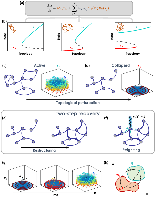
Figure 1: Reviving a failed network. (a) The components of our modeling framework: network structure/weights are captured by $A$ and $W$ (grey terms); interaction mechanisms are described by $M_{0}(x),M_{1}(x),M_{2}(x)$ (orange terms). (b) Depending on the dynamics - e.g., cellular, neuronal or microbial - the system exhibits distinct fixed-points, active ($\mathbf{x}_{1}$, green) or failed ($\mathbf{x}_{0}$, red). Transitions between these states are driven by perturbations to $A,W$. (c) Unperturbed, the system resides in $\mathbf{x}_{1}$, where all $x_{i}>0$. In this presentation, here and throughout, the network nodes are laid out on the $x,y$ plane, and their activities $x_{i}$ are captured by the $z$ coordinate. Hence, an active system has all nodes spread along the positive $z$-axis, while a failed network is laid-out around $z\to 0$. We also use color coding from red (small $x_{i}$) to blue (large $x_{i}$) as visual aid. (d) Perturbations to $A,W$, such as node/link removal or weight reduction, result in a collapse to the inactive $\mathbf{x}_{0}$. For this system, under $\mathbf{x}_{0}$, all activities vanish ($z=0$). (e) Step I. Restructuring. To revive the failed system we first restructure $A,W$ to a point where it can recover, namely a point where $\mathbf{x}_{1}$ is potentially stable. (f) Step II. Reigniting. After restructuring we revive the active state $\mathbf{x}_{1}$ by controlling a microscopic set of nodes, here the single node $s$. Externally forcing $s$ to sustain constant activity $x_{s}(t)=\Delta$, we drive the network towards $\mathbf{x}_{1}$. (g) Following reigniting ($x_{s}(t)=\Delta$, black node at center), the forcing signal gradually spreads, until the system’s activity $\mathbf{x}_{1}$ is restored. (h) In this process we use the natural basin structure of our dynamics. To reignite $\mathbf{x}_{1}$ we steer the system from $\mathfrak{B}_{0}$ (red) to any point within $\mathfrak{B}_{1}$ (green). Once in $\mathfrak{B}_{1}$, we cease our forcing, and the system naturally transitions to the desired $\mathbf{x}_{1}$ (dashed arrows).

Complex systems, biological, social or technological, often experience perturbations and disturbances, from overload failures in power systems ^{1, 2, 3} to species extinction in ecological networks. ^{4, 5, 6} The impact of such perturbations is often subtle, the system exhibits a minor response, but continues to sustain its global functionality. ^{7, 8} However, in extreme cases, a large enough perturbation may lead to a major collapse, with the system abruptly transitioning from a functional to a dysfunctional dynamic state ^{9, 10, 11, 12, 13} (Fig. 1a-d). When such collapse occurs, the naïve instinct is to reverse the damage, retrieve the failed nodes and reconstruct the lost links. This, however, is seldom efficient, as (i) we rarely have access to all system components, ¹⁴ limiting our ability to reconstruct the perturbed network; (ii) even if we could reverse the damage, due to hysteresis, in many cases, the system will not spontaneously regain its lost functionality.

To address this challenge, we derive here a two-step recovery process: Step I. Restructuring (Fig. 1e). Retrieving the weighted topology to a point where the system can potentially regain its functionality. Step II. Reigniting (Fig. 1f). Introducing dynamic interventions to steer the system back to its functional state. Considering the fact that in most practical scenarios we cannot control the majority of the system components, we design our reigniting around micro-interventions, i.e. controlling just a small number of components. To achieve this we uncover the recoverable phase, a dynamic state in which the system can be driven towards functionality by controlling just a single node.

The challenge of irreversible collapse

Consider a complex system of $N$ components (nodes), interacting via the adjacency matrix $A$, a sparse, potentially directed random network with an arbitrary degree distribution $P(k_{\rm in},k_{\rm out})$ (see Supplementary Section 1). Each node is assigned an activity $x_{i}(t)$, whose meaning depends on context - e.g., a species abundance in a microbial network or a gene’s expression level in a biological setting. We then track the evolution of $x_{i}(t)$ following ^{15, 16, 17}

$$\mathinner{\dfrac{\operatorname{d\!}{}x_{i}}{\operatorname{d\!}{t}}}=M_{0}\big{(}x_{i}(t)\big{)}+\sum\limits_{j=1}^{N}A_{ij}W_{ij}M_{1}\big{(}x_{i}(t)\big{)}M_{2}\big{(}x_{j}(t)\big{)},$$ (1)

in which the interaction dynamics is characterized by three potentially nonlinear functions $M_{0}(x),M_{1}(x)$ and $M_{2}(x)$. The first function, $M_{0}(x_{i})$ captures node $i$’s self-dynamics, describing mechanisms such as protein degradation ¹⁸ (cellular), individual recovery ¹⁹ (epidemic) or birth/death processes ²⁰ (population dynamics). The product $M_{1}(x_{i})M_{2}(x_{j})$ describes the $i,j$ interaction mechanism, e.g., genetic activation, ²¹ infection ¹⁹ or symbiosis. ²² The strength of the $i,j$ interaction is governed by $W_{ij}$, a random weight extracted from the density function $P(w)$, whose average we denote by $\omega=\int_{0}^{\infty}wP(w)\operatorname{d\!}w$.

In the context of recoverability, we seek to revive the activity of all nodes by activating a selected set of nodes, hence we focus on cooperative interactions, in which nodes positively contribute to each others activity. This is expressed in Eq. (1) through $W_{ij}M_{1}(x_{i})M_{2}(x_{j})\geq 0$ (Supplementary Section 1). Later, in our discussion of the microbiome recoverability, we relax this condition and examine the impact of mixed-sign interactions.

Setting the derivative on the l.h.s. of (1) to zero, we obtain the system’s fixed-points, $\mathbf{x}_{\alpha}=(x_{\alpha,1},\dots,x_{\alpha,N})^{\top}$, which, if dynamically stable, represent different states, desirable or undesirable, in which the system can naturally reside. Transitions between these states often result from perturbations to $A$ or $W$, such as node/link deletion or reduction in link weight. When this occurs, it is difficult to reverse the unwanted transition. This is because the system often avoids spontaneous recovery, even if we retrieve the lost nodes, links or weights. To illustrate this difficulty we refer to a concrete example below.

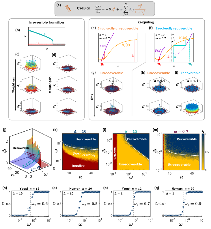
Figure 3: Recoverability of cellular dynamics. (a) The Michaelis-Menten model for sub-cellular dynamics. (b) The average activity $\bar{x}$ vs. the weight reduction $q$ ($q=0$ - no reduction). $\mathbf{x}_{1}$ is only stable for $q\leq q_{c}$ (green); $\mathbf{x}_{0}$ is always stable (red). (c) We track $x_{i}$ for three specific values of $q$. For small $q$ (top) all $x_{i}>0$, an active state $\mathbf{x}_{1}$. As $q$ increases $x_{i}$ become smaller (center), until the system collapses into the inactive $\mathbf{x}_{0}$ (bottom). (d) Retrieving the lost weights does not revive the system since $\mathbf{x}_{0}$ is always stable. To revive the failed system we apply single-node reigniting: (e) $F(x)$ (purple) and $M_{2}(x)$ (yellow) as obtained from the left/right hand sides of Eq. (9) with $\kappa=3,\omega=0.7,\rho=1$. We observe Case 1 of Fig. 2c, with a single intersection at $\mathfrak{B}_{0}$ (red). This describes a structurally unrecoverable system. (f) Under a denser $A$ ($\kappa=10$), $F(x)$ changes form and the system now follows Case 3 - structurally recoverable with $\Delta_{c}=1$ (vertical dashed-line). (g) Forcing $s$ (black node) to a permanent $\Delta$ activity, no matter how large, fails to reignite the structurally unrecoverable system of panel e. (h) - (i) Reigniting fails for $\Delta=0.9$, but succeeds for $\Delta=1.1$, confirming our predicted $\Delta_{c}=1$ in panel f. (j) The $\kappa,\omega,\Delta$ phase-space. The red area in $\kappa,\omega$ captures the structurally unrecoverable regime. We show three specific cross-sections, fixing $\Delta$ (blue), $\kappa$ (green) and $\omega$ (red), to be expanded in panels k-m. (k) The $\kappa,\omega$ phase-diagram, as obtained from $5\times 10^{4}$ scale-free networks (Supplementary Section 5.3). Each data-point represents the fraction $\eta$ of successful reigniting instances across $20$ independent attempts. We observe the predicted phases: inactive (red), where only $\mathbf{x}_{0}$ is stable, unrecoverable ($\eta=0$, yellow), and recoverable ($\eta=1$, blue), where single-node reigniting is possible. Our theoretical prediction is also shown (white solid line). (l) - (m) The $\omega,\Delta$ and $\kappa,\Delta$ diagrams. For $\omega<0.6$ (l) and for $\kappa<8$ (m) the system is structurally unrecoverable, and hence $\Delta_{c}\to\infty$. The theoretical prediction is also shown (white solid lines). (n) - (o) $\eta$ vs. $\omega$ as obtained from the Yeast and Human protein interaction networks ($\kappa=12$ and $29$; $\Delta=10$). For $\omega<\omega_{c}$ (vertical dashed-lines) reigniting fails ($\eta=0$), above it - it is successful ($\eta=1$), as predicted. (p) - (q) Similar results under $\Delta=1$.

Example 1. Cellular dynamics (Fig. 3). As our first example we consider the Michaelis-Menten model for gene-regulation, capturing activation interactions between genes (Fig. 3a). Here $M_{0}(x_{i})=-Bx_{i}^{a}$, $M_{1}(x_{i})=1$ and $M_{2}(x_{j})=x_{j}^{h}/(1+x_{j}^{h})$, a switch-like function that saturates to $M_{2}(x_{j})\rightarrow 1$ for large $x_{j}$, representing the process of activation (see discussion in Supplementary Section 3.1).

For sufficiently connected $A$ or large average weight $\omega$ the system exhibits an active state $\mathbf{x}_{1}$, in which all $x_{1,i}>0$ - capturing a living cell. However, perturbations to $A,W$, such as link/node removal or weight loss can cause a sharp transition to the inactive state $\mathbf{x}_{0}=(0,\dots,0)^{\top}$, i.e. cell death. To track this transition systematically we measured the average activity $\bar{x}_{\alpha}=(1/N)\sum_{i=1}^{N}x_{\alpha,i}$, which follows $\bar{x}_{\alpha}>0$ for $\alpha=1$ and $\bar{x}_{\alpha}=0$ for $\alpha=0$. As we subject the system to increasing levels of stress - here, reducing all weights $W$ by a factor $0\leq q\leq 1$, we observe a sudden transition at $q=q_{c}$ from $\mathbf{x}_{1}$ (Fig. 3b, green) to $\mathbf{x}_{0}$ (red). Next, we attempt to revive the node activities by retrieving the lost weights, finding that the system fails to recover. The reason is that while $\mathbf{x}_{1}$ is only stable under $q\leq q_{c}$, $\mathbf{x}_{0}$ is always stable - both below and above this threshold. This leads to a hysteresis phenomenon, where the system remains inactive despite the reversal of the perturbation.

Example 1, above, while representing a specific scenario, illustrates the family of challenges that we tackle here: system’s with irreversible transitions, driven by perturbations to their weighted topology. To revive such systems, we must not just restructure their lost topology, but also dynamically reignite them by exerting external control over the activities $x_{i}(t)$.

Recoverability

The most natural way to reignite the system is to drive all activities $x_{i}$ towards an initial condition from which the system naturally recovers to the desired $\mathbf{x}_{1}$. Namely, we must steer the system into $\mathbf{x}_{1}$’s basin of attraction

$$\mathfrak{B}_{1}=\Big{\{}\mathbf{x}(t=0)\,\,\Big{|}\,\,\mathbf{x}(t\rightarrow\infty)=\mathbf{x}_{1}\Big{\}}$$ (2)

which comprises all initial conditions $\mathbf{x}(t=0)$ from which Eq. (1) converges to $\mathbf{x}(t\rightarrow\infty)=\mathbf{x}_{1}$ (Fig. 1h). The problem is that such level of control over the dynamics of all nodes is seldom attainable, hence we seek to recover the system’s functionality by driving just a microscopic fraction $f\rightarrow 0$ of forced nodes.

To achieve this, we consider the limit $f\sim 1/N$, in which case our reigniting is attempted through, typically, a single, randomly selected source node $s$, whose activity we force to follow $x_{s}(t)=\phi(t)$. In many practical applications our ability to exert such control, even on a single node, is restrictive, limiting the potential forms of $\phi(t)$. Hence, below we reignite (1) using an extremely simple input, $\phi(t)={\rm Const}$. Other practically accessible forms of $\phi(t)$ are further considered in Supplementary Section 4. As simple as it is, the constant forcing itself is also constrained, as our forcing capacity is, often, bounded by $\phi(t)\leq\Delta$. Hence, below we seek the conditions where such restricted interventions - controlling just one node and with a forcing bounded by $\Delta$ - can push the remaining nodes into the desired $\mathfrak{B}_{1}$.

During our intervention, the remaining $N-1$ nodes continue to follow the natural system dynamics, i.e. Eq. (1), as they respond to the $s$-forcing. In technical terms, the failed state of the system, $\mathbf{x}_{0}$, captures Eq. (1)’s initial condition, and the forced node imposes a strict boundary condition at $s$. In a recoverable system, after some time, the activities will enter $\mathfrak{B}_{1}$, at which point we can cease our external control and allow the system to naturally transition to $\mathbf{x}_{1}$, following its internal dynamics. If, however, the system is non-recoverable, such single-node reigniting is insufficient, the system remains at $\mathfrak{B}_{0}$, and once we lift our forcing, it relaxes back to $\mathbf{x}_{0}$, a failed reigniting.

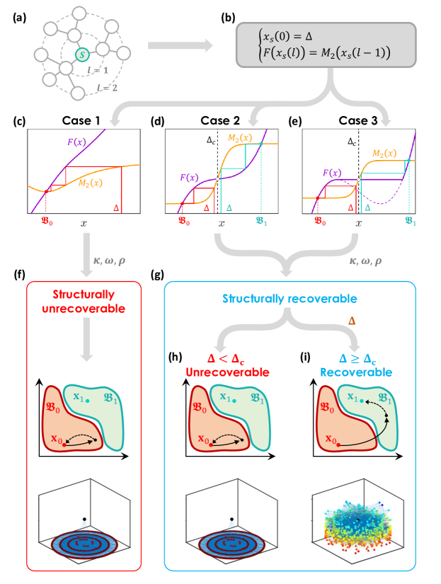
Figure 2: Can a system be reignited by a single node? (a) During reigniting we select a single source node $s$ and, for a limited time, artificially force it to sustain a permanent activity $\Delta$. To track the system’s response, we divide the network into shells $K_{s}(l)$ comprising all nodes at distance $l$ from $s$. (b) The average activity $x_{s}(l)$ of all nodes at $K_{s}(l)$ follows the recurrence relation of Eq. (5), starting from our forcing at $s$ (top equation), and tracking its propagation as it penetrates the network shells (bottom equation). Successful reigniting requires $x_{s}(l\rightarrow\infty)\in\mathfrak{B}_{1}$, i.e. that the distant shells were driven towards the desired basin. (c) - (e) To track the convergence of the recurrence relation we plot $F(x)$ (purple) and $M_{2}(x)$ (yellow). The forcing $\Delta$ determines our initial starting point, and the recurrence follows the red or green trajectories. The final state $x_{s}(l\rightarrow\infty)$ is reached when the two functions, $F(x)$ and $M_{2}(x)$, intersect. We observe three potential scenarios (Supplementary Section 2.5): Case 1. $F(x)$ and $M_{2}(x)$ have a single intersection in $\mathfrak{B}_{0}$ (red). Under these conditions, regardless of $\Delta$ the recurrence converges to $\mathbf{x}_{s}(l\rightarrow\infty)\in\mathfrak{B}_{0}$, and hence the system is structurally unrecoverable. Case 2. $F(x)$ and $M_{2}(x)$ exhibit two intersections, corresponding to the system’s two stable fixed points $\mathbf{x}_{0}$ (red) and $x_{1}$ (green); the intermediate intersection (white dot) is unstable. Here, for $\Delta<\Delta_{c}$ the system converges to $\mathfrak{B}_{0}$, i.e. unrecoverable (red trajectory), while for $\Delta\geq\Delta_{c}$ it approaches $\mathfrak{B}_{1}$ - hence it is recoverable (green trajectory). Case 3. In case $F(x)$ is non-monotonic the critical forcing $\Delta_{c}$ is determined by $F(x)$’s local maximum point, see Supplementary Section 2.5 for a detailed analysis of Case 3. (f) Structural recoverability is determined by the network topology $A,W$ through $\kappa,\omega$ and $\rho$. A structurally unrecoverable (Case 1) system remains confined to $\mathfrak{B}_{0}$ and hence cannot be revived, even under arbitrarily large $\Delta$. (g) A structurally recoverable system (Cases 2,3) is unrecoverable if $\Delta<\Delta_{c}$ (left), and recoverable otherwise (right). Hence, the recoverable-phase is driven by three structural parameters ($\kappa,\omega,\rho$, grey) and a single dynamic parameter ($\Delta$, orange).

To analytically track the system’s response to our forcing at $s$, we divide the rest of the network into shells $K_{s}(l)=\{j\,\,|\,\,L_{sj}=l\}$, comprising all nodes located at distance $l$ from $s$ (Fig. 2a). In this notation $K_{s}(0)=\{s\}$, $K_{s}(1)$ is the group of $s$’s nearest outgoing neighbors, $K_{s}(2)$ its next neighbors, and so on. Then, starting with $x_{s}(t)=\Delta$, we track the average activity of nodes in $K_{s}(l)$, via

$$x_{s}(l,t)=\dfrac{1}{|K_{s}(l)|}\sum_{i\in K_{s}(l)}x_{i}(t),$$ (3)

where $|K_{s}(l)|$ represents the number of nodes in $K_{s}(l)$. The shells adjacent to the source (small $l$) will be forced to respond to $s$’s activation $\Delta$. The distant shells, however, at $l\to\infty$, may be unaffected, and therefore still within $\mathfrak{B}_{0}$. Under these conditions, upon termination of our $\Delta$-forcing, all shells retreat back to $\mathbf{x}_{0}$, rendering the system unrecoverable. Successful reigniting, therefore, requires that

$$x_{s}(l\to\infty,t\to\infty)\in\mathfrak{B}_{1},$$ (4)

capturing a state in which the forcing at $s$ was able to penetrate the network and affect the activity of even the most distant nodes at $K_{s}(l\rightarrow\infty)$. This represents a recoverable system that will naturally revert to $\mathbf{x}_{1}$ once the forcing $\Delta$ is deactivated. ²³

To obtain the final shell states $x_{s}(l)=x_{s}(l,t\to\infty)$, we use the fact that, despite its potentially broad degree/weight distribution, our network is otherwise wired, and assigned link weights, at random (Supplementary Section 1). Therefore, (i) $A$ features insignificant degree-correlations, and hence the nodes in $K_{s}(l)$ are statistically similar to those in $K_{s}(l^{\prime})$, (for $l,l^{\prime}\geq 1$); (ii) $A$ is locally tree-like, and therefore, asymptotically, there are almost no short-range loops surrounding the source $s$. Below we relax both approximations, when testing our method, numerically, against empirically constructed networks, which, indeed, feature both loops and measurable degree-correlations (Supplementary Section 5.5). However, to advance analytically, we use approximations (i) and (ii) to translate Eq. (1) into a direct set of equations for $x_{s}(l)$. We arrive the recurrence relation (Supplementary Section 2)

$$\begin{cases}x_{s}(0)=\Delta,\\[5.0pt] F\big{(}x_{s}(l)\big{)}=M_{2}\big{(}x_{s}(l-1)\big{)},\end{cases}$$ (5)

where

$$F(x)=\dfrac{1}{\omega}R(x)-\rho\kappa M_{2}\left(R^{-1}\left(\omega M_{2}(x)+\omega\kappa M_{2}(\bar{\mathbf{x}}_{0})\right)\right)-(1-\rho)\kappa M_{2}\big{(}\bar{\mathbf{x}}_{0}\big{)},$$ (6)

$R(x)=-M_{0}(x)/M_{1}(x)$ and $R^{-1}(x)$ is its inverse function. In (6) the parameter $\bar{\mathbf{x}}_{0}$ represents the mean activity of nodes in $K_{s}(l>1)$ under the failed state $\mathbf{x}_{0}$ (Supplementary Section 2.4). The remaining parameters are extracted directly from the weighted topology $A,W$: $\omega$ is is the average weight,

$$\kappa=\dfrac{1}{N}\sum_{i=1}^{N}\frac{1}{|K_{i}(1)|}\sum_{j=1}^{N}A_{ij}^{\top}k_{j,\rm in}-1,$$ (7)

represents the average neighbor’s residual in-degree, ^{24, 13} and $\rho=P(A_{ij}=1|A_{ij}^{\top}=1)$ describes the network’s reciprocity, i.e. the probability to observe a link $i\to j$, given the existence of $j\to i$ (for undirected networks $\rho=1$).

Equations (5) and (6) represent our key result. They approximate the recoverability of (1), a multidimensional nonlinear dynamic equation, through a manageable first order recurrence relation. This recurrence takes the system’s weighted topology ($\kappa,\rho,\omega$) and its nonlinear dynamics ($M_{0},M_{1},M_{2}$) as input, and, together with our intervention constraints ($\Delta$), predicts the system’s recoverability as output. Indeed, for any given forcing $\Delta$, the recurrence (5) either converges to $x_{s}(l\rightarrow\infty)\in\mathfrak{B}_{1}$, satisfying the recoverability condition (4), or to $x_{s}(l\rightarrow\infty)\in\mathfrak{B}_{0}$, indicating a failed recovery.

To obtain $x_{s}(l\rightarrow\infty)$ we extract the stationary states of (5), requiring

$$F(x)=M_{2}(x),$$ (8)

which in turn provides $x_{s}(l)=x_{s}(l-1)$. ^{25, 26} Depending on $\kappa,\omega$ and $\rho$, we observe two characteristic behaviors (Fig. 2, Supplementary section 2.5): Structurally unrecoverable (Fig. 2c,f). In case $F(x)$ and $M_{2}(x)$ have a single intersection $x\in\mathfrak{B}_{0}$, then the series in (5) inevitably converges to that point. This captures structural unrecoverability, in which regardless of $\Delta$, single-node reigniting is prohibited. Structurally recoverable (Fig. 2d,e,g). If, on the other hand, $F(x)$ and $M_{2}(x)$ have several intersections, then the convergence of Eq. (5) depends on the boundary condition $x_{s}(0)=\Delta$, whose magnitude is determined by our forcing capacity. For $\Delta<\Delta_{c}$, our forcing is too small, and the system approaches $\mathfrak{B}_{0}$, a failed reigniting. For $\Delta\geq\Delta_{c}$ it will reach $\mathfrak{B}_{1}$, capturing a successful reigniting. The recoverable-phase (Fig. 2i). If a system is structurally recoverable and $\Delta\geq\Delta_{c}$ we say that it is in the recoverable-phase, a state in which one can revive the system by forcing just one node.

Taken together, for a given dynamics $M_{0}(x),M_{1}(x),M_{2}(x)$, our formalism predicts a four-dimensional phase-diagram in the $\kappa,\rho,\omega,\Delta$ phase-space, helping us identify the boundaries of recoverability. Next we investigate this phase space on a range of relevant systems, from cellular dynamics (Example 1), to neuronal and microbial systems. In our first examples below, we consider, for simplicity, undirected networks ($\rho=1$), reducing our phase-space to three relevant dimensions, $\kappa,\omega$ and $\Delta$. Our final example, reviving a dysfunctional microbiome, examines recoverability under directed interactions ($\rho<1$).

Applications

Example 1. Cellular dynamics (Fig. 3; Supplementary Section 3.1). As our first application we return to Example 1, regulatory dynamics, where $M_{0}(x)=-x^{a},M_{1}(x)=1$ and $M_{2}(x)=x^{h}/(1+x^{h})$, and therefore $R(x)=x^{a}$ and $R^{-1}(x)=x^{1/a}$. Equation (8) under $\rho=1$ becomes

$$\dfrac{1}{\omega}x^{a}-\dfrac{\kappa x^{\frac{h^{2}}{a}}}{x^{\frac{h^{2}}{a}}+\omega^{-\frac{h}{a}}{\big{(}1+x^{h}\big{)}^{\frac{h}{a}}}}=\dfrac{x^{h}}{1+x^{h}},$$ (9)

whose roots ($x$) determine the potential fixed-points of the reignited system. Clearly, $x=0$ is a solution, capturing the fact that the failed state $\mathbf{x}_{0}=(0,\dots,0)^{\top}\in\mathfrak{B}_{0}$ is always stable. Hence, the question is, under what conditions do we observe a second solution $x>0$, representing a potential convergence to $\mathfrak{B}_{1}$. To answer this, in Fig. 3e,f we plot $M_{2}(x)$ vs. $x$ (yellow) and observe its intersections with $F(x)$ (purple) as we vary the values of $\kappa,\omega$. This allows us to observe, graphically, the potential convergence of the system to $\mathfrak{B}_{0}$ or $\mathfrak{B}_{1}$.

First we consider $\kappa=3,\omega=0.7$ (Fig. 3e). We find that (9) exhibits only one solution, represented by the single intersection at $x=0$ (red dot). This guarantees that (5) converges to $x_{s}(l\rightarrow\infty)=0$, independently of $\Delta$. Consequently, the system is structurally unrecoverable. Indeed, Fig. 3g indicates that, despite the forcing $\Delta$ at $s$, the system fails to reactivate.

Increasing the network density to $\kappa=10$, however, changes the picture, as now (9) features three intersection points (Fig. 3f): an intermediate unstable point (white) and two stable points at $x=0$ (red) and at $x>0$ (green), representing convergence to $\mathfrak{B}_{0}$ and $\mathfrak{B}_{1}$, respectively. Hence now the system is structurally recoverable, with critical forcing $\Delta_{c}=1$ (vertical dashed line), above which it enters the recoverable-phase. This prediction is corroborated in Fig. 3h,i: under $\Delta=0.9$ the system remains in $\mathfrak{B}_{0}$, but for $\Delta=1.1$, just above $\Delta_{c}$, it successfully reignites, precisely as predicted.

This uncovers the existence of a previously overlooked dynamic phase of the Michaelis-Menten model. Indeed, the regulatory system of Fig. 3a has been previously ¹³ shown to follow two phases, inactive, where only $\mathbf{x}_{0}$ is stable vs. bi-stable where both $\mathbf{x}_{0}$ and $\mathbf{x}_{1}$ are stable (Fig. 3b-d). Yet we now unveil a third phase: recoverable, a subspace of the bi-stable phase, in which the system can be reignited from $\mathbf{x}_{0}$ to $\mathbf{x}_{1}$ by controlling a single node.

To examine this phase-space systematically, in Fig. 3j we present the recoverability phase-diagram. For small $\kappa,\omega$ we observe the structurally unrecoverable regime, in which recoverability is unattainable even with arbitrarily large $\Delta$ (red patch in the $\kappa,\omega$ plane). The remaining area in $\kappa,\omega$ represents the structurally recoverable regime, which is split between the unrecoverable phase, for $\Delta<\Delta_{c}$ (below surface), and the recoverable phase when $\Delta\geq\Delta_{c}$ (above surface).

Setting $\Delta$ constant, in Fig. 3k we construct the $\omega,\kappa$ phase-diagram, by numerically simulating regulatory dynamics on an ensemble of $5\times 10^{4}$ scale-free networks, covering $2,500$ distinct combinations of $\omega$ and $\kappa$ (Supplementary Section 5.3). Each data-point captures the fraction of successful recoveries $\eta$ among $20$ independent reigniting trails, from zero successes ($\eta=0$, yellow) to $100\%$ successful recovery attempts ($\eta=1$, blue). The white solid line represents our theoretical prediction, based on analyzing the intersections of (9). We find that the boundaries of recoverability (yellow/blue) can be well-approximated by our analytical framework. We also present the $\omega,\Delta$ and $\kappa,\Delta$ phase diagrams, further confirming our predicted transitions (Fig. 3l,m).

To test our predictions in an empirical setting, we collected data on two real biological networks, capturing protein interactions in Human ²⁷ ($\kappa=29$) and Yeast ²⁸ ($\kappa=12$) cells. Varying $\omega$ and $\Delta$ we measured the reigniting success rate $\eta$, observing in both networks the sharp transition into the recoverable phase (Fig. 3n-q), which falls precisely on the theoretically predicted phase boundary ($\omega_{c}$, vertical dashed lines).

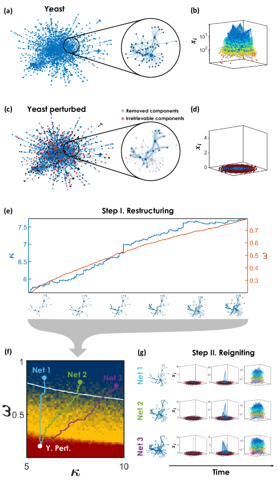
Figure 4: Two-step recovery for reviving a failed cellular system. (a) The unperturbed Yeast protein interaction network. For visibility we focus on the circled sub-network. (b) As expected, the unperturbed network is in the active state $\mathbf{x}_{1}$, hence all $x_{i}>0$. (c) - (d) Following extensive perturbation in which $30\%$ of nodes/links (grey and red) were deleted the state of the network collapses to the inactive $\mathbf{x}_{0}$, i.e. all $x_{i}=0$. The challenge is that some of the deleted components (nodes/links) are inaccessible, and hence cannot be retrieved (red). This captures restructuring constraints that are, indeed, inevitable in realistic scenarios. Circle at center - we focus on the same sub-network shown in panel a, the deleted nodes/links appear in grey and red, the remaining unperturbed components are highlighted, . (e) Step I. Within the given constraints we restructure the network by reintroducing nodes/links or strengthening link weights. We map these interventions into their impact on the two relevant control parameters $\kappa$ (blue) and $\omega$ (orange). For illustration, we show the highlighted sub-network of panel c as it restructures, acquiring nodes, links and increased weights (sub-networks along the $x$-axis). (f) Restructuring paths in the $\kappa,\omega$ phase-diagram. A successful path leads the network from the collapsed phase (red) into the recoverable-phase (blue). Using our predicted phase-diagram we design several alternative paths, affording us flexibility to, e.g., focus on increasing weights $\omega$ (Net 1, light-blue path) or also on enhancing network density $\kappa$ (Net 3, purple path), all depending on the nature of our constraints. (g) Step II. Once the network is in the recoverable-phase, we can revive it via single-node reigniting, demonstrated here on each of our restructured networks, Net 1-3.

Restructuring guidelines (Fig. 4). In case our system is not in the recoverable phase, we must design appropriate restructuring interventions to push $\omega$ or $\kappa$ towards recoverability. In a cellular environment this can be achieved through biochemical interventions that help catalyze or inhibit specific reactions. ²⁹ The phase-diagrams of Fig. 3j-m, mapping the boundaries of the recoverable-phase, can help us design such interventions.

To illustrate this, in Fig. 4a-d we simulate a cellular network (Yeast) that has been driven towards inactivity due to a series of node/link deletion (grey nodes/links). Some of the removed components are inaccessible (red), and hence cannot be retrieve during restructuring. With these constraints in mind, we incorporate our two-step strategy: Step I. Restructuring. We design a sequence of accessible interventions on $A,W$ to bring the network closer to the recoverable phase. An example of such a sequence is shown in Fig. 4e (along the $x$-axis). On the $y$-axis we present the accumulating impact of these restructuring interventions on $\kappa$ (blue) and $\omega$ (orange). To revive the system, we seek paths of such accessible interventions that help deliver the network into the bounds of the recoverable-phase (Fig. 4f). Our goal, we emphasize, is not to simply retrieve the lost components, but to achieve recoverability. This designates, not a single point, but rather an entire sub-space in $\kappa,\omega$ (Fig. 4f, blue area), affording us some level of restructuring flexibility. Indeed, despite the network’s irretrievable components, we were able to design three distinct restructuring paths, leading to different destinations - Net 1,2 or 3 - all within the recoverable sub-space (blue area). Step II. Reigniting. Once in the recoverable phase we can revive the system via single-node reigniting as shown in Fig. 4g for Net 1,2 and 3.

This example illustrates how the phase-diagrams of recoverability provide guidelines for restructuring. For example, in Fig. 4f path $1$ builds mainly on controlling the interaction strengths ($\omega$), but assumes little freedom to add nodes or links ($\kappa$). In contrast path $3$ involves a significant component of adding nodes/links to $A$, affecting not just $\omega$ but also $\kappa$. The optimal restructuring path is, therefore, determined by the nature of our constraints, e.g., the relative difficulty in adding weights vs. adding nodes/links. While the potential space of structural interventions in Step I is incomprehensibly vast, our phase-diagrams reduce this space into just two relevant control parameters - $\kappa$, characterizing $A$’s density, and $\omega$, capturing its link weights (and $\rho$ in case $A$ is directed). This reduction allows us to asses the contribution of all potential interventions by quantifying their effect on these two (or three) parameters - providing optimal pathways towards recoverability (see further discussion in Supplementary Section 3.1.3).

Example 2. Neuronal dynamics (Fig. 5; Supplementary Section 3.2). As our second example we consider the Wilson-Cowan neuronal dynamics, ^{30, 31} in which (1) follows the form shown in Fig. 5a. ^{32, 33} The system naturally exhibits two dynamic states (Fig.5b): suppressed ($\mathbf{x}_{0}$, red) in which all activities are constricted; active ($\mathbf{x}_{1}$, green) where $x_{i}$ are relatively large (green). In between these two extremes lies a bi-stable-phase, in which both $\mathbf{x}_{0}$ and $\mathbf{x}_{1}$ are potentially stable (grey shaded). This predicts a hysteresis phenomenon, in which a system driven to the left of the grey area will avoid spontaneous recovery.

To observe the predicted phases, in Fig. 5c we numerically analyze our ensemble of $5\times 10^{4}$ scale-free networks. We find, indeed, the active (green) and suppressed (red) phases, separated by the strip of bi-stability (grey). Our formalism, however, predicts an additional dynamic phase - recoverable. This phase, shown in Fig. 5d,e (blue area) identifies a sub-space within the bi-stable regime, under which the system can be driven to $\mathbf{x}_{1}$ via single-node reigniting. The theoretically predicted phase boundaries are also shown (white solid lines), precisely capturing the numerically observed transitions (yellow/blue).

In the Methods Section we further demonstrate how the brain’s modular structure impacts the recoverability phase-space. We also characterize conditions under which modularity provides a fail-safe mechanism, in which one module revives the other upon failure.

Example 3. Microbial dynamics (Fig. 6, Supplementary Section 3.3). As our final example we consider the gut-microbiome, a microbial community, whose functional state has been shown to crucially impact human health. ^{34, 35} Following perturbations, such as antibiotic treatment, the abundance of the different species may reach critical levels, potentially leading to a dysfunctional microbiome. ³⁶ We, therefore, examine below how our two-step revival strategy can help steer a failed microbiome back to functionality.

To construct the interaction network, we collected data ³⁷ describing the metabolic in/out flux of $N=838$ microbial species, allowing us to map their complementary chemical interactions. A cooperative link $i\to j$ appears when species $i$ produces a resource consumed by $j$; ³⁸ an adversarial link $i\leftrightarrow j$ is assigned if $i$ and $j$ both compete over the same resource. ³⁹ The weight $W_{ij}$ of each link captures the level of inter-species reliance: for example, if $i$ is the sole producer of $j$’s only consumed nutrient $m$, then $j$’s growth strongly depends on $i$. If, however, there are many alternative producers of $m$, or if $m$ is just one of $j$’s many consumed nutrients, then $W_{ij}$ will be small. We arrive at a directed and highly diverse network with broadly distributed weights, and most crucially, with $\sim 75\%$ adversarial interactions, i.e. $W_{ij}<0$ (Fig. 6b,c, Supplementary Section 3.3.3). This challenges our theoretical framework, which is primarily designed around cooperative interactions, and therefore helps us test its applicability limits.

To track the microbial populations we used the dynamics shown in Fig. 6a. The self-dynamics combines logistic growth with the Allee effect, ⁴⁰ and the inter-species cooperative/adversarial interactions follow the Lotka-Volterra dynamics. ²² The parameter $F$ captures the externally introduced microbial influx. Of the original pool of $N$ species, we find that $32\%$ cannot be supported by the network and undergo extinction. The remaining $568$ species, comprising the actual microbiome composition, exhibit two potential fixed-points (Fig. 6d-f), a functional $\mathbf{x}_{1}$ and a dysfunctional $\mathbf{x}_{0}$. Our goal is to apply our two-step recoverability strategy to drive a dysfunctional microbiome at $\mathbf{x}_{0}$ back towards $\mathbf{x}_{1}$.

Selective reigniting. In the Methods Section we show how to evaluate each node’s reigniting capacity $\mathcal{R}_{s}$, allowing us to rank all candidate reigniter species in the microbiome, based on their potential to revive the system (Fig. 6g,h). For a random topology, where all shells $K_{s}(l)$ are statistically similar, we expect minor differences in $\mathcal{R}_{s}$ between the nodes. Here, however, we find that $\mathcal{R}_{s}$ is highly diverse, with the top $26$ species having $\mathcal{R}_{s}>300$, and the remaining species with $\mathcal{R}_{s}$ one or two orders of magnitude below (Fig. 6i). Such diversity, a consequence of the unique non-random structure of the microbiome, indicates that, in this system, the top $26$ nodes represent preferred candidates for reigniting. To examine this, we attempted reigniting the microbiome with all nodes sequentially, finding that, indeed, success was by far more likely among the top ranked reigniters (Fig. 6j-l, see also Methods).

One exception we identify among these top reigniters is P. putida, which despite having $\mathcal{R}_{s}=359$, ranking $6$ in the reigniters list, still falls short of reviving the system (Fig. 6k). This is due to the fact that P. putida’s reigniting capacity is hindered by its many surrounding adversarial interactions. Indeed, reigniting, by its nature, builds on the positive activation that the source species $s$ exerts on its neighbors at $K_{s}(l)$. Such positive impact is undermined by negative links. Next, we use P. putida’s restricted reigniting capacity as an opportunity to examine our two-step strategy in a realistic setting.

Two-step recovery of a dysfunctional microbiome (Fig. 6m-q). Consider a microbial network at state $\mathbf{x}_{0}$, which we wish to recover. Among the many practical constraints on our potential interventions, one crucial constraint is that we lack control over the majority of microbial species, and hence we must achieve recovery with a handful of accessible reigniting nodes. Specifically, let us assume that our top accessible candidate for reigniting is precisely P. putida, which, as Fig. 6k indicates, by itself, cannot revive the system. Hence we employ our two-step strategy. Step I. Restructuring. To enhance P. putida’s reigniting capacity we wish to inhibit the adversarial interactions, which stand in the way of the system’s reactivation. We consider two potential interventions: (i) Removing selected nodes that have many adversarial interactions (competition hubs) by means of targeted narrow spectrum antibiotic treatment. (ii) Deleting or weakening adversarial links through nutritional or biological interventions. ^{41, 42} For example, if $i$ and $j$ compete over metabolite $m$, we prescribe dietary supplements to ensure the availability of $m$, thus eliminating the $i,j$ competitive interaction (Fig. 6m). Since antibiotic intervention on an already dysfunctional microbiome may cause additional risks, here, we implement restructuring via option (ii). First, we rank all nutrients based on their relative contribution to the adversarial weights in $W$ (Fig. 6n, Supplementary Section 3.3.3). We then supplement the top three nutrients in the list (green) to restructure the network. Eliminating the competition over these, now freely available nutrients, we arrive at our restructured network, which, thanks to our interventions, has now a more suitable balance of cooperative vs. adversarial interactions (Fig. 6o). Step II. Reigniting. In the microbiome, forcing can be implemented by administering probiotics, a common therapeutic practice that helps sustain, artificially, a desired abundance of a selected species. ⁴³ The rate of the probiotic intake determines the average activation force, set to be above the reigniting threshold $\Delta_{c}$. Having restructured the network, we now attempt, once again, to reignite it with P. putida. We find that the originally failed reigniter, is now, capable of reviving the inactive microbiome (Fig. 6p,q).

Applicability limits. Our theoretical analysis helps construct the precise phase-diagrams in the $\kappa,\omega,\Delta$ space, predicting the bounds of the recoverable-phase. These analytically tractable observations rely on a specific set of assumptions, mainly, that $A$ features little degree-correlations and has a scarcity of short-range loops, and that the dynamics is of the form (1) and has primarily cooperative interactions. A precise description of these modeling assumptions is provided in Supplementary Section 1.

Our applications, however, provide insights that extend well beyond these analytical limits. For example, our empirical networks, cellular, neuronal and microbial, all exhibit non-negligible deviations from the above assumptions, and yet, our analysis correctly predicted their recoverability (Supplementary Section 5.5). The gut-microbiome analysis helped us derive implementable guidelines for reigniting, including also the notion of selective reigniting, despite the network’s strong degree-correlations and significant share of adversarial links (Fig. 6). In Supplementary Section 3.4 we further consider diffusive interactions, in which the governing equation is generalized beyond the form of Eq. (1). We also analyze alternative forms of reigniting, using periodic activity boosts, which in certain applications may be more accessible than the time-independent forcing ($\Delta$) considered here (Supplementary Section 4).

Discussion and outlook

While the structure of complex networks has been deeply investigated over the years, our understanding of their dynamics is still emerging. The challenge is often focused on prediction, aiming to foresee a network’s dynamic behavior. Here, we go a step further, and focus on influence, showing how to steer a system towards a desired behavior.

Our solution seals a crucial gap in our pursue of nonlinear system controllability. ⁴⁴ Existing approaches often rely on specific system symmetries, ^{45, 46, 47} which do not cover complex systems of the form (1). Absent such symmetries, complex system control is frequently studied by means of linearization, ^{48, 49} using the linear approximation to help capture the system’s local behavior in the vicinity of each of its fixed-point. Such local analysis, however, is insufficient in the context of recoverability, as here we seek to drive the system outside of its current basin and hence beyond the linear regime. To overcome this restriction of locality, cross-basin control was recently developed using time-varying inputs, that adapt until the system is pushed - step by step - into the desired basin of attraction. ¹⁴ While highly effective, such interventions require a detailed control over the nodes’ dynamics, first, monitoring the system’s response, then updating, in real-time, the form of our intervention. Such level of observation/control is not always guaranteed.

To break this gridlock, we seek non-local control, i.e. across basins, but with simple dynamic interventions, that do not require highly detailed input signals. Our recoverablity phase-diagram addresses this by identifying unique conditions where such control is attainable. On the one hand, pushing the system across basins, but on the other hand, using an extremely crude and simple control input - a time-limited constant activation $\Delta$ that is applied to just one or few nodes. No fine-tuning or real-time updating of the input signal is required. Indeed, all that is needed is a strong enough jolt to the system, after which it naturally relaxes to its desired target state.

The microscopic behavior of complex networks is driven by countless parameters, from the fine-structure of $A$ and $W$ to the specific rates of each node’s dynamic processes. Our analysis, however, shows, that their large-scale functionality can be traced to a manageable set of relevant parameters, i.e. $\kappa,\omega,\rho$ and $\Delta$. Such dimension reduction is the fundamental premise of statistical-physics, allowing to analyze systems with endless degrees of freedom using a limited set of statistical entries. We believe, that such an approach to network dynamics, can help us understand, predict, and ultimately influence the behavior of these complex multi-dimensional systems.

Acknowledgments. HS wishes to thank the support of the President fellowship of Bar-Ilan University, Israel, and the Mordecai and Monique Katz Graduate Fellowship Program. This research was supported by the Israel Science Foundation (grant no. 499/19 and 189/19), the US National Science Foundation-CRISP award (grant no. 1735505), the Bar-Ilan University Data Science Institute grant for research on network dynamics, the Binational Israel-China Science Foundation (grant no. 3132/19), the US-Israel NSF-BSF program (grant no. 2019740), the EU H2020 project RISE (grant no. 821115), the EU H2020 project DIT4TRAM (grant no. 953783) and the Defense Threat Reduction Agency (DTRA grant no. HDTRA-1-19-1-0016).

Author contributions. All authors designed the research. HS and BB conducted the mathematical analysis. HS performed the numerical simulations and analyzed the data. AB supervised the microbiome analysis. BB was the lead writer of the paper.

Competing interests. The authors declare no competing interests.

Data availability. Empirical data required for constructing the real-world networks (Microbiome, Brain, Yeast PPI, Human PPI) will be uploaded to a freely accessible repository upon publication.

Code availability. All codes to reproduce, examine and improve our proposed analysis will be made freely available online upon publication.

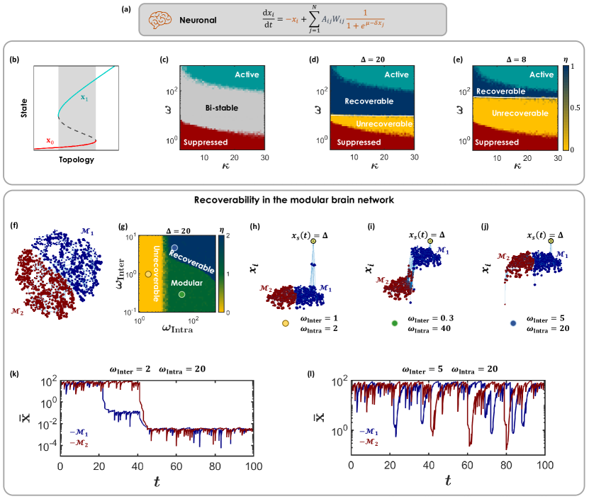
Figure 5: Recoverability of neuronal dynamics. (a) The Wilson-Cowan neuronal dynamics. ³³ (b) The system exhibits three states: suppressed $\mathbf{x}_{0}$ (red) when $\kappa,\omega$ are small; active $\mathbf{x}_{1}$ (green) under large $\kappa,\omega$; bi-stable (center, grey shaded) in which both $\mathbf{x}_{0}$ and $\mathbf{x}_{1}$ are stable. (c) The three states, suppressed (red), active (green) and bi-stable (grey), as obtained from $5\times 10^{4}$ scale-free networks capturing distinct combinations of $\kappa,\omega$. (d) - (e) The $\kappa,\omega$ recoverability phase-diagram under $\Delta=20$ and $\Delta=8$. Each data-point represents $20$ independent realizations. As predicted, the bi-stable state is split into two distinct dynamic phases - unrecoverable (yellow) vs. recoverable (blue). Simulation results (yellow-blue transition) are in perfect agreement with our theoretical predictions (white solid lines). (f) The empirically constructed brain network, and its two hemispheres $\mathcal{M}_{1}$ (blue) and $\mathcal{M}_{2}$ (red). (g) We measured the reigniting success rate $\eta$ of the modular brain network along the $\omega_{\rm Intra},\omega_{\rm Inter}$ phase-diagram (see Methods). We observe three phases: unrecoverable, in which no module can be revived ($\eta=0$, yellow); recoverable, in which both modules reactivate ($\eta=2$, blue); modular, in which reigniting is constrained to a single module ($\eta=1$, green). (h) Setting $\omega_{\rm Inter}=1,\omega_{\rm Intra}=2$, in the unrecoverable phase (yellow circle), we find, indeed, that reigniting fails to revive both modules. (i) In the modular phase (green circle), $\mathcal{M}_{1}$ recovers, but fails to reactivate $\mathcal{M}_{2}$. (j) In the recoverable phase (blue circle) reigniting successfully crosses over from $\mathcal{M}_{1}$ to $\mathcal{M}_{2}$. (k) The average activity $\bar{\mathbf{x}}$ of $\mathcal{M}_{1}$ (blue) and $\mathcal{M}_{2}$ (red) vs. $t$, as obtained from numerically simulating neuronal dynamics on the brain network. Adding noise, we observe sporadic fluctuations, some causing a transition to the suppressed state. The first collapse occurs to $\mathcal{M}_{1}$ at $t\sim 20$. Soon after, $\mathcal{M}_{2}$ also collapses at $t\sim 40$, and the entire network irreversibly fails. (l) Increasing the inter-module weights to $\omega_{\rm Inter}=5$, we enter the recoverable phase. Now when one module fails, the other module reignites it. This captures a fail-safe system, whose modular structure provides internally embedded self-recoverability.

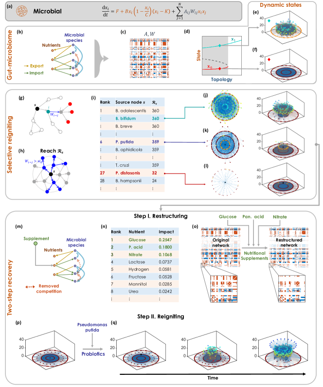
Figure 6: Recoverability of microbial dynamics. (a) Population dynamics. (b) The export (orange) import (green) network, linking microbial species to the nutrients they produce/consume. Cooperative links (blue) are assigned when $i$’s exports are imported by $j$; adversarial links (red) - when $i$ and $j$ share mutual import/s. (c) The resulting gut-microbiome, a diverse weighted and directed network with mixed cooperative (blue) and adversarial (red) links. (d) - (f) The system exhibits two states, the functional $\mathbf{x}_{1}$ (green diamond) or the dysfunctional $\mathbf{x}_{0}$ (red diamond), with a broad range of bi-stability (grey shaded) (g) The propagation of a reigniting signal: $s\to i\to j$. In Methods we show that an effective $i\to j$ link must satisfy $W_{i\to j}>w_{0}$. (h) Counting only effective links, we obtain $s$’s reigniting capacity $\mathcal{R}_{s}$, as the number potentially reactivated nodes (blue). (i) We ranked all microbial species based on $\mathcal{R}_{s}$, identifying the network’s most effective reigniters. The top $26$ nodes stand out with $\mathcal{R}_{s}$ orders of magnitude higher than the rest. (j) The visibly dense effective network surrounding B. bifidum ($\mathcal{R}_{s}=360$). As expected, B. bifidum successfully reignites the microbiome (right). (k) - (l) We examined two lower ranked species, which failed to revive the network. Specifically, P. putida, despite having high $\mathcal{R}_{s}$, causes only a local impact but fails to revive the network. (m) To reignite with P. putida we employ our two-step strategy. In Step I, we use nutritional supplements (green) to eliminate competitive links (red dashed-link) by ensuring nutrient availability (n) We ranked nutrients based on their contribution to the adversarial links. The top three ranking nutrients are highlighted (green). (o) Supplementing these three nutrients via dietary interventions, we restructure the microbial network, reducing adversarial interactions (red). See insets for visible comparison. (p) In step 2 we administer probiotics to boost the population of a specific species. (q) After restructuring we find that P. putida, an originally failed reigniter, can now successfully revive the microbiome.

Methods

Recoverability of modular networks. Applying our formalism to an empirically constructed brain network, ¹ allows us to examine its predictive power beyond our analytical assumptions of a random $A$. Indeed, the brain, with its two hemispheres, provides a highly structured (non-random) modular network, partitioned into two clearly distinctive communities $\mathcal{M}_{1}$ and $\mathcal{M}_{2}$ (Fig. 5f). It, therefore, offers meaningful insights on recoverability across modules. The question is, can reigniting one module, say $\mathcal{M}_{1}$, spillover to also revive $\mathcal{M}_{2}$. Our analysis indicates that this depends on the average strength of the links within the modules, $\omega_{\rm Intra}$, vs. that of the links between the two modules, $\omega_{\rm Inter}$ (Fig. 5g). Clearly, if $\omega_{\rm Intra}$ is too small, then both $\mathcal{M}_{1}$ and $\mathcal{M}_{2}$ are, in and of themselves, unrecoverable, and reigniting will inevitably fail (Fig. 5h). If both $\omega_{\rm Intra}$ and $\omega_{\rm Inter}$ are sufficiently large, then the reactivated nodes at $\mathcal{M}_{1}$ will further reignite their neighbors at $\mathcal{M}_{2}$, allowing a complete recovery of both modules via single-node reigniting (Fig. 5j). In between these two extremes, we observe a third phase, in which reigniting is confined to $\mathcal{M}_{1}$, but fails to penetrate $\mathcal{M}_{2}$ (Fig. 5i).

The result is a three state phase-space, as shown in Fig. 5g: recoverable (blue), in which reigniting at $\mathcal{M}_{1}$ can reactivate also $\mathcal{M}_{2}$, unrecoverable (yellow), in which both modules cannot be revived, and modular (green), where $\mathcal{M}_{1}$ recovers, but the reigniting signal fails to penetrate $\mathcal{M}_{2}$. To construct the phase-diagram of Fig. 5g we simulated neuronal dynamics on the brain network of Fig. 5f, scanning $2,500$ distinct combinations of $\omega_{\rm Intra}$ and $\omega_{\rm Inter}$. For each combination we attempted $20$ independent realizations of reigniting with randomly selected nodes. We then extracted $\eta$, as the average number of revived modules over the $20$ attempts. Hence, $\eta=0$ means that no module was revived (yellow), and $\eta=1$ indicates that (on average) reigniting was restricted to only the source node’s module (green), but did not cross over to the other module. Finally, if $\eta=2$ then both modules were reactivated (blue).

This observation highlights the potential benefits of network modularity for self-recovery. Indeed, if one module fails, say $\mathcal{M}_{2}$, the other module, $\mathcal{M}_{1}$, if still active, can revive it. This is because $\mathcal{M}_{1}$’s active nodes can themselves help reignite the inactive $\mathcal{M}_{2}$. Hence, modularity offers a fail-safe network architecture, in which, unless both modules simultaneously fail, one module can reactivate the other. This ensures a sustained activity in the face of sporadic failures. To observe this we simulated neuronal dynamics on our brain network, setting the inter-modular link weights to $\omega_{\rm Inter}=2$. Starting at $\mathbf{x}_{1}$, we introduce external noise, that causes the activity of both modules to fluctuate, until a sufficiently large perturbation, occurring at random around $t\sim 20$, leads $\mathcal{M}_{1}$ to irreversibly fail (Fig. 5k, blue). Shortly after, a similar fate meets $\mathcal{M}_{2}$ (red) and the entire system collapses to $\mathbf{x}_{0}$.

We now repeat the exact same experiment, this time with $\omega_{\rm Inter}=5$, bringing the system into the fully recoverable-phase ($\eta=2$, blue). Now, at every instance in which, say $\mathcal{M}_{1}$ fails, $\mathcal{M}_{2}$’s active nodes reignite it back into activity (Fig. 5l). Hence, modularity can afford the system a fail-safe dynamics, driven by its capacity for self-recoverability.

Selective reigniting in the microbiome. A unique aspect of the our empirically constructed microbiome network, is that it deviates significantly from a random topology. Indeed, in a random network, as degree-correlations are negligible, the statistical properties of the shells $K_{s}(l)$ become approximately independent of $s$ for $l>1$. In simple terms, while nodes may have diverse degrees, i.e. $K_{s}(1)\neq K_{s^{\prime}}(1)$, their second or third neighbors at $K_{s}(l>1)$ are statistically similar. Under these conditions, once a system is in the recoverable phase, one can reignite it using any desired node, as, indeed, all nodes have roughly identical shells in their surrounding. If, however, the environments $K_{s}(l)$ vary significantly across the nodes, we expect that certain nodes become better reigniters than others. This gives rise to selective reigniting, in which the system’s recoverability is not just a function of the network, but also depends on the specific source node $s$ and its unique reigniting capacity.

Consider the reigniting signal as it propagates from the source $s$, and penetrates through the shells $K_{s}(1),K_{s}(2),\dots$. At a certain instance it revives a node $i\in K_{s}(l)$, then advances from $i$ to impact its neighbor $j\in K_{s}(l+1)$ and so on (Fig. 6g). In Supplementary Section 3.3.3 we show that such propagation across shells, namely that a revived $i$ can, indeed, reactivate its more distant neighbor $j$, requires that the $i\to j$ link weight exceeds a threshold $w_{0}$. Hence, the links whose weight $W\geq w_{0}$, constitute effectual links, that help propagate the reigniting signal. The remaining links with $W<w_{0}$ have but a marginal contribution to the reigniting. We, therefore, construct an effective network, comprising only the effectual links (Fig. 6h, blue links/nodes). This, more selective, network represents the relevant set of interactions that actively participate in the reigniting process. Constructing this network we obtain the effectual shells surrounding each node $s$, whose number of nodes captures $s$’s reigniting capacity $\mathcal{R}_{s}$. Nodes with large $\mathcal{R}_{s}$ are surrounded by many effectual links, and therefore they have a higher reigniting capacity.

In a random topology, where all shells are statistically similar, we expect minor differences in $\mathcal{R}_{s}$ between the nodes. In the microbiome, however, we find that $\mathcal{R}_{s}$ is highly diverse, with the top $26$ species having $\mathcal{R}_{s}>300$, and the remaining species with $\mathcal{R}_{s}$ that is one or two orders of magnitude below (Fig. 6i). Such diversity, a consequence of the unique structure of the microbiome, indicates that, in this system, the top $26$ nodes represent preferred candidates for reigniting. To examine this in Supplementary Fig. 7 we show $\eta$ vs. the $\mathcal{R}_{s}$-ranking for all nodes in the microbiome. We clearly observe that the top ranked nodes have a much higher probability to successfully reignite the system.

References

- 1 P. Van Mieghem. Graph Spectra for Complex Networks. Cambridge University Press, Cambridge, UK, 2010.
- 2 J. Zhao, D. Li, H. Sanhedrai, R. Cohen and S. Havlin. Spatio-temporal propagation of cascading overload failures in spatially embedded networks. Nature Communications, 7:10094 – 99, 2016.
- 3 I. Dobson, B.A. Carreras, V.E. Lynch and D.E. Newman. Complex systems analysis of series of blackouts: Cascading failure, critical points, and self-organization. Chaos, 17:026103, 2007.
- 4 H.-Y. Shih, T.-L. Hsieh and N. Goldenfeld. Ecological collapse and the emergence of travelling waves at the onset of shear turbulence. Nature Physics, 12(3):245–248, 2016.
- 5 J. Jiang, A. Hastings and Y.-C. Lai. Harnessing tipping points in complex ecological networks. Journal of the Royal Society Interface, 16(158):20190345, 2019.
- 6 R.M. May. Thresholds and breakpoints in ecosystems with a multiplicity of stable states. Nature, 269:471–477, 1977.
- 7 R. Cohen, K. Erez, D. Ben-Avraham and S. Havlin. Breakdown of the internet under intentional attack. Physical Review Letters, 86(16):3682, 2001.
- 8 H.I. Schreier, Y. Soen and N. Brenner. Exploratory adaptation in large random networks. Nature Communications, 8(1):1–9, 2017.
- 9 A.E. Motter and Y.-C. Lai. Cascade-based attacks on complex networks. Physical Review E, 66:065102, 2002.
- 10 P. Crucitti, V. Latora and M. Marchiori. Model for cascading failures in complex networks. Physical Review E, 69:045104–7, 2004.
- 11 D. Achlioptas, R.M. D’Souza and J. Spencer. Explosive percolation in random networks. Science, 323:1453–1455, 2009.
- 12 S. Boccaletti, J.A. Almendral, S. Guana, I. Leyvad, Z. Liua, I.S. Nadal, Z. Wang and Y. Zou. Explosive transitions in complex networks’ structure and dynamics: Percolation and synchronization. Physics Reports, 660:1–94, 2016.
- 13 J. Gao, B. Barzel and A.-L. Barabási. Universal resilience patterns in complex networks. Nature, 530:307––312, 2016.
- 14 S.P. Cornelius, W.L. Kath and A.E. Motter. Realistic control of network dynamics. Nature Communications, 4:1942–1950, 2013.
- 15 B. Barzel and A.-L. Barabási. Network link prediction by global silencing of indirect correlations. Nature Biotechnology, 31:720 – 725, 2013.
- 16 U. Harush and B. Barzel. Dynamic patterns of information flow in complex networks. Nature Communications, 8:2181, 2017.
- 17 C. Hens, U. Harush, R. Cohen, S. Haber and B. Barzel . Spatiotemporal propagation of signals in complex networks. Nature Physics, 15:403, 2019.
- 18 B. Barzel and O. Biham. Binomial moment equations for stochastic reaction systems. Physical Review Letters, 106:150602–5, 2011.
- 19 R. Pastor-Satorras, C. Castellano, P. Van Mieghem and A. Vespignani. Epidemic processes in complex networks. Rev. Mod. Phys., 87:925–958, 2015.
- 20 T.S. Gardner, C.R. Cantor and J.J. Collins. Construction of a genetic toggle switch in escherichia coli. Nature, 403:339, 2000.
- 21 G. Karlebach and R. Shamir. Modelling and analysis of gene regulatory networks. Nature Reviews, 9:770–780, 2008.
- 22 C.S. Holling. Some characteristics of simple types of predation and parasitism. The Canadian Entomologist, 91:385–398, 1959.
- 23 Note that in Eq. (4) we use the sign loosely, as strictly speaking, includes initial conditions of the form , not scalar averages such as . Hence, Eq. (4) should be taken to mean: the shell average is congruent with a state .
- 24 M.E.J. Newman. Networks - an introduction. Oxford University Press, New York, 2010.
- 25 R.M. May. Simple mathematical models with very complicated dynamics. Nature, 261:459–467, 1976.
- 26 S.H. Strogatz. Nonlinear dynamics and chaos with student solutions manual: With applications to physics, biology, chemistry, and engineering. CRC press, 2018.
- 27 J.F. Rual et al. Towards a proteome-scale map of the human protein-–protein interaction network. Nature, 437:1173–1178, 2005.
- 28 H. Yu et al. High-quality binary protein interaction map of the yeast interactome network. Science, 322:104–110, 2008.
- 29 P.K. Robinson. Enzymes: principles and biotechnological applications. Essays in biochemistry, 59:1, 2015.
- 30 H.R. Wilson and J.D. Cowan. Excitatory and inhibitory interactions in localized populations of model neurons. Biophysical Journal, 12(1):1–24, 1972.
- 31 H.R. Wilson and J.D. Cowan. A mathematical theory of the functional dynamics of cortical and thalamic nervous tissue. Kybernetik, 13(2):55–80, 1973.
- 32 E. Laurence, N. Doyon, L.J. Dubé and P. Desrosiers. Spectral dimension reduction of complex dynamical networks. Physical Review X, 9(1):011042, 2019.
- 33 We use a modified version of the model, which can be cast if the form of Eq. (1). See discussion in Supplementary Section 3.2.
- 34 A.L. Gould, V. Zhang, L. Lamberti, E.W. Jones, B. Obadia, N. Korasidis, A. Gavryushkin, J.M. Carlson, N. Beerenwinkel and W.B. Ludington. Microbiome interactions shape host fitness. Proceedings of the National Academy of Sciences, 115(51):E11951–E11960, 2018.
- 35 L. García-Bayona and L.E. Comstock. Bacterial antagonism in host-associated microbial communities. Science, 361(6408), 2018.
- 36 B.P. Willing, S.L. Russell and B.B. Finlay. Shifting the balance: antibiotic effects on host–microbiota mutualism. Nature Reviews Microbiology, 9(4):233–243, 2011.
- 37 R. Lim, J.J.T. Cabatbat, T.L.P. Martin, H. Kim, S. Kim, J. Sung, C.-M. Ghim and P.-J. Kim. Large-scale metabolic interaction network of the mouse and human gut microbiota. Scientific Data, 7(1):1–8, 2020.
- 38 J. Kehe, A. Ortiz, A. Kulesa, J. Gore, P.C. Blainey and J. Friedman. Positive interactions are common among culturable bacteria. bioRxiv, 2020.
- 39 R. Levy and E. Borenstein. Metabolic modeling of species interaction in the human microbiome elucidates community-level assembly rules. Proceedings of the National Academy of Sciences, 110(31):12804–12809, 2013.
- 40 W. C. Allee, O. Park, A.E. Emerson, T. Park and K.P. Schmidt. Principles of animal ecology. 1949.
- 41 E.K. Costello, K. Stagaman, L. Dethlefsen, B.J. Bohannan and D.A. Relman. The application of ecological theory toward an understanding of the human microbiome. Science, 336(6086):1255–1262, 2012.
- 42 B.B. Hsu, T.E. Gibson, V. Yeliseyev, Q. Liu, L. Lyon et al. Dynamic modulation of the gut microbiota and metabolome by bacteriophages in a mouse model. Cell host & microbe, 25(6):803–814, 2019.
- 43 R. El Hage, E. Hernandez-Sanabria and T. Van de Wiele. Emerging trends in “smart probiotics”: functional consideration for the development of novel health and industrial applications. Frontiers in microbiology, 8:1889, 2017.
- 44 Y.Y Liu and A.-L. Barabási. Control principles of complex systems. Reviews of Modern Physics, 88(3):035006, 2016.
- 45 A. Isidori, E.D. Sontag, and M. Thoma. Nonlinear Control Systems, volume 3. Springer, 1995.
- 46 R. Hermann and A. Krener. Nonlinear controllability and observability. IEEE Transactions on Automatic Control, 22(5):728–740, 1977.
- 47 A.J. Whalen, S.N. Brennan, T.D. Sauer and S.J. Schiff. Observability and controllability of nonlinear networks: The role of symmetry. Physical Review X, 5(1):011005, 2015.
- 48 J.-M. Coron. Control and nonlinearity. Number 136. American Mathematical Soc., 2007.
- 49 E.D. Sontag. Mathematical control theory, volume 6 of texts in applied mathematics, 1998.

References

- 1 E. Bullmore and O. Sporns. Complex brain networks: graph theoretical analysis of structural and functional systems. Nature reviews neuroscience, 10(3):186–198, 2009.