Progress in the Glauber model at collider energies

Abstract

We review the theoretical and experimental progress in the Glauber model of multiple nucleon and/or parton scatterings, after the last 10–15 years of operation with proton and nuclear beams at the CERN Large Hadron Collider (LHC) and with various light and heavy colliding ions at the BNL Relativistic Heavy Ion Collider (RHIC). The main developments and the state-of-the-art of the field are summarized. These encompass measurements of the inclusive inelastic proton and nuclear cross sections, advances in the description of the proton and nuclear density profiles and their fluctuations, inclusion of subnucleonic degrees of freedom, experimental procedures and issues related to the determination of the collision centrality, validation of the binary scaling prescription for hard scattering cross sections, and constraints on transport properties of quark-gluon matter from varying initial-state conditions in relativistic hydrodynamics calculations. These advances confirm the validity and usefulness of the Glauber formalism for quantitative studies of QCD matter produced in high-energy collisions of systems, from protons to uranium nuclei, of vastly different size.

1 INTRODUCTION

The central goal of high-energy nucleus-nucleus (AA) collisions is to study the collective thermodynamic and transport properties of quarks and gluons, the elementary degrees of freedom of the theory of strong interaction (Quantum Chromodynamics, QCD) [1]. Colliding heavy-ions at center-of-mass (c.m.) energies above tens of GeV is the only experimental way known to produce a large multibody system of deconfined partons, the quark-gluon plasma (QGP), predicted by lattice QCD calculations for energy densities exceeding a critical value of $\upepsilon_{\rm c}\approx$ 0.5 GeV/fm³ [2, 3]. Such collisions provide the only available means to study the thermodynamics of a non-Abelian quantum gauge field theory in the laboratory.

Larger transverse spatial overlaps of the two incoming ions lead to a larger volume of the created system thereby resulting in “mesoscopic” conditions conductive to partial (local) thermalization and subsequent collective behavior of the produced partons. Hence, the interpretation of data from high-energy heavy-ion collisions relies on a detailed knowledge of the initial QGP matter distribution, resulting from the overlap of the two nuclei colliding at a given impact parameter ($b$), complemented with a theoretical modeling of its subsequent spacetime evolution. Deriving from the data the transverse size of the created QGP, as well as any event-by-event irregularities arising from density and/or color fluctuations, is crucial to interpret the experimental observations, because the total and local depositions of energy in the collision chiefly influence the initial conditions and the evolution of the produced strongly-interacting system.

The generic method to study the properties of QCD matter relies on measuring the distributions of a variety of observables in AA collisions, and compare them to the same measurements in proton-proton (pp) and/or proton-nucleus (pA) collisions, where a QGP is not expected to be produced. Common observables include particle production yields (light hadrons, heavy-quarks, quarkonia, jets, photons, etc.) as functions of their transverse momentum ($p_{\rm T}$), pseudorapidity ($\eta$), azimuthal angle ($\phi$) [4]. Carrying out such quantitative comparisons among colliding systems of different sizes requires appropriate normalization of the measured distributions by using e.g. the number of participating nucleons ($N_{\rm part}$), the number of independent binary nucleon-nucleon (NN) collisions ($N_{\rm coll}$), the medium transverse area ($A_{\perp}$), or the system eccentricity $\epsilon_{n}$ (given by the $n^{\rm th}$ moments of its azimuthal spatial distribution), as described below.

Computing the aforementioned quantities typically relies on describing multiple scatterings of the constituents (nucleons, themselves characterized by parton densities) inside the colliding nuclei, using the so-called Glauber formalism, named after Roy Glauber’s pioneering work on the use of quantum mechanical scattering theory to calculate cross sections in pA and AA collisions [5, 6]. The Glauber formalism is based on the geometric or eikonal approximation, which assumes projectile nucleons to travel along straight lines (i.e. with negligible momentum exchanges compared to their longitudinal momenta) and to undergo multiple independent subcollisions with nucleons in the target. In the original form of the Glauber approach [7, 8, 9], the total hadronic cross section of a collision of two nuclei (with $A$ and $B$ number of nucleons, respectively) is given by a $(2A+2B+1)$-dimensional integral

$$\sigma_{\rm AB}=\int{\rm d}^{2}b\int{\rm d}^{2}{\rm s}^{\rm A}_{1}\cdots{\rm d}^{2}{\rm s}^{\rm A}_{A}{\rm d}^{2}{\rm s}^{\rm B}_{1}\cdots{\rm d}^{2}{\rm s}^{\rm B}_{B}\times$$

$$T_{{}_{\rm A}}({\bf s}^{\rm A}_{1})\cdots T_{{}_{\rm A}}({\bf s}^{\rm A}_{A})T_{{}_{\rm B}}({\bf s}^{\rm B}_{1})\cdots T_{{}_{\rm B}}({\bf s}^{\rm B}_{B})\times$$ (1)

$$\left\{1-\prod_{j=1}^{B}\prod_{i=1}^{A}\left[1-{\sigma}({\bf b}-{\bf s}^{\rm A}_{i}+{\bf s}^{\rm B}_{j}\right]\right\}\;,$$

where ${\bf b}$ is the collision impact parameter and ${\bf s}$ denotes a position in the transverse plane. The interaction probability ${\sigma}({\bf s})$ is normalized to give the nucleon–nucleon inelastic cross section $\sigma_{\rm NN}=\int{\rm d}^{2}{\rm s}\,{\sigma}({\bf s})$. The nuclear thickness function ${T}_{\rm A}({\bf b})=\int{\rm d}z\,\rho_{A}({\bf b},z)$ describes the transverse nucleon density by integrating the nuclear density $\rho$ along the longitudinal direction ($z$).

In the so-called optical limit of the Glauber model derived in [9], local density fluctuations and correlations are ignored so that each nucleon in the projectile interacts with the incoming target as a flux tube described with a smooth density. The total cross section then reduces to

$$\sigma_{\rm AB}=\int{\rm d}^{2}b\left\{1-\left[1-\sigma_{\rm NN}T_{{}_{\rm AB}}({\bf b})\right]^{AB}\right\}\;,$$ (2)

where

$$T_{{}_{\rm AB}}\left(\bf{b}\right)=\int{{\rm d}^{2}{\rm s}\;T_{{}_{\rm A}}\left(\bf{s}\right)T_{{}_{\rm B}}\left(\bf{s}-\bf{b}\right)}$$ (3)

is known as the nuclear overlap function, normalized as $\int{\rm d}^{2}b\;T_{{}_{\rm AB}}(b)=A\,B$ by integrating over all impact parameters. Expressions (1) and (2) give identical results for large enough nuclei and/or for sufficiently small values of $\sigma_{\rm NN}$.

In contrast to optical calculations, Monte Carlo Glauber (MCG) calculations [10, 11, 12, 13, 14, 15, 16, 17, 18, 19] evaluate the phase space of Eq. (1) stochastically by distributing the $A,B$ nucleons of nucleus A and B, respectively, in coordinate space according to their corresponding nuclear densities, separated by an impact parameter $b$ sampled from $\mathrm{d}\sigma/\mathrm{d}b\propto b$. The nuclear transverse profiles are usually approximated with parametrizations of charge density distributions extracted from low-energy electron-nucleus scattering experiments [20, 21] that, for large spherical nuclei, are usually described by 2-parameter Fermi (2pF) (also called Woods-Saxon) distributions, $\rho(r)=\rho_{0}/(1+\exp(\frac{r-R}{a}))$, with half-density radius $R$ and diffusivity $a$. Following the eikonal approximation, the collision is treated as a sequence of independent binary nucleon-nucleon collisions, i.e. the nucleons travel on straight-line trajectories and their interaction probability does not depend on the number of collisions they have suffered before. In its simplest form, an interaction takes place between two nucleons if the distance $d$ between their centers satisfies $d<\sqrt{\sigma_{\rm NN}/\pi}$. Alternatives to this so-called “black disk” approximation, using for example a Gaussian-like distribution for the nucleon overlap or more complex forms, are also used as discussed below.

One of the most typical phenomenological applications of the Glauber model is to provide the initial conditions for the number density (or entropy or energy densities, related to the former via the QCD equation of state, EoS) of the medium formed in nuclear collisions as input for hydrodynamic calculations of its subsequent space-time evolution. The initial entropy profile in the transverse plane at midrapidity ($\eta=0$) is typically assumed to be proportional to a linear combination of the number density of particles produced in soft (with yields assumed to scale as the $N_{\rm part}$ pairs) and hard (scaling as $N_{\rm coll}$) scatterings [22]

$$s_{0}(\vec{r}_{\perp})\equiv\frac{dS}{\tau_{0}\,{\rm d}^{2}r_{\perp}{\rm d}\eta}\bigg{|}_{\eta=0}=\frac{C}{\tau_{0}}\left(\frac{1-\alpha}{2}\,\rho_{\rm part}(\vec{r}_{\perp})+\alpha\,\rho_{\rm coll}(\vec{r}_{\perp})\right)\,,$$ (4)

with the relative weight often taken as $\alpha=0.2$ at the LHC. Two typical snapshots in the $(x,y)$ plane of the medium formed in PbPb and pPb collisions at the LHC are shown in Fig. 1. Right after the collision, the spectator nucleons (in grey in the figure) continue undisturbed with the original longitudinal momenta inside the beam line, whereas the hot and dense QGP formed at midrapidity at the LHC expands longitudinally (transversely) at about (0.6 times) the speed of light.

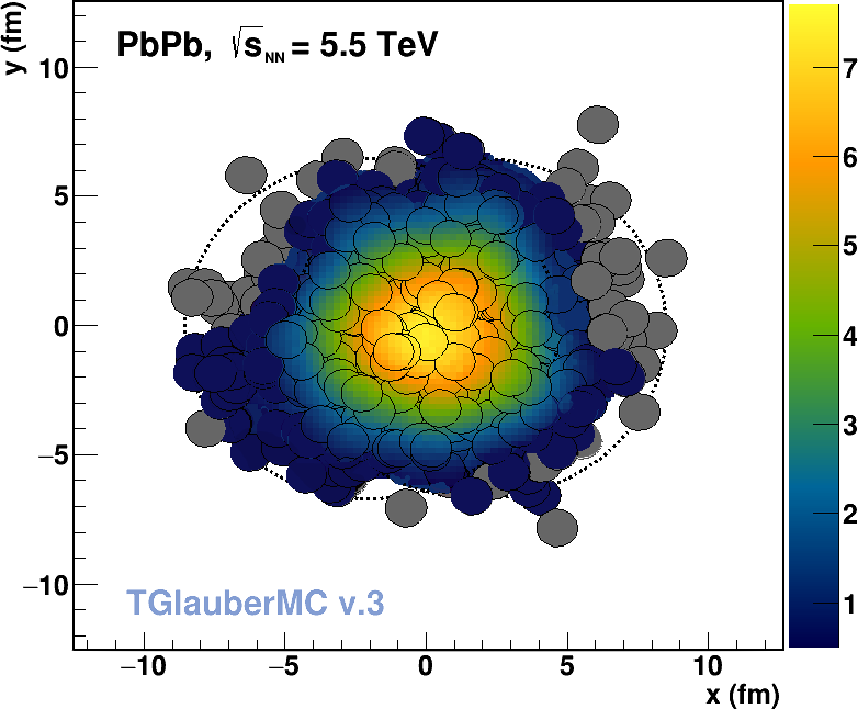
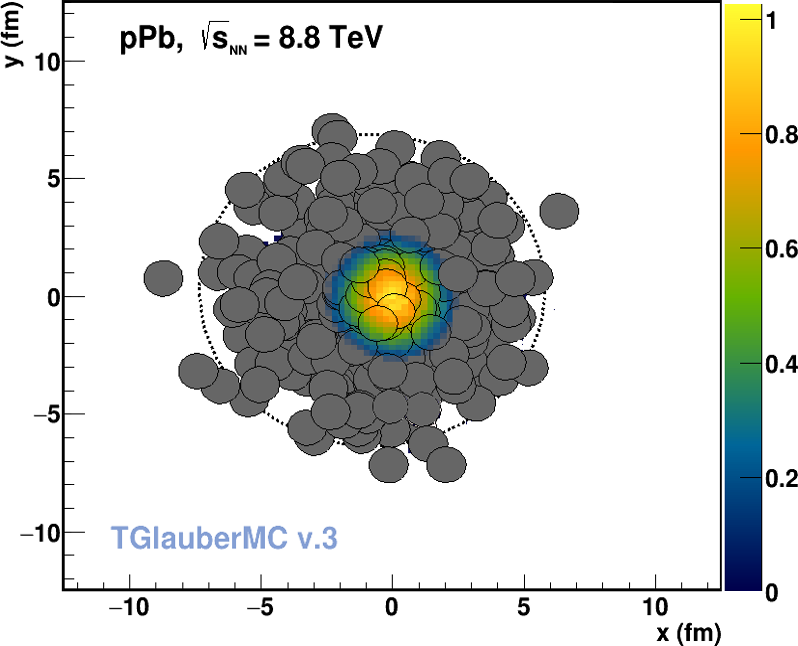
Figure 1: Events displays of initial transverse density profiles in the $(x,y)$ plane of PbPb collisions at $\!\sqrt{s_{{}_{\rm NN}}}=5.5$ TeV with a triangular-like shape (5–10% centrality, left), and pPb at $\!\sqrt{s_{{}_{\rm NN}}}=8.8$ TeV (0–1% centrality, right) generated with TGlauberMC [18]. The colored bidimensional surfaces indicate the local density (fm^-2), following the weighting given by Eq. (4) with $\alpha=0.2$. The grey circles indicate spectator nucleons that do not participate in the collision process.

Among the quantities derived from Glauber models, the initial azimuthal anisotropy of the QGP system is an important one as it directly propagates to various flow components in the final state through collective hydrodynamic pressure gradients, and is thereby particularly sensitive to the transport and thermodynamic properties of QCD matter [23]. The harmonics eccentricities $\epsilon_{n}$ of the produced QGP (with $n=2$ being its ellipticity, $n=3$ triangularity, etc.) are theoretically defined as

$$\epsilon_{n}\equiv\frac{\left|\int r^{n}e^{in\phi}\,w(r,\phi)rdrd\phi\right|}{\int r^{n}\,w(r,\phi)rdrd\phi}\,,$$ (5)

where the weights $w(r,\phi)$ are often taken as the initial density of the medium derived from the Glauber model itself via a linear combination of the underlying $N_{\rm part}$ and $N_{\rm coll}$ distributions, as in Eq. (4). Assuming linear hydrodynamics response, the final harmonic flows determined from the azimuthal distributions of the produced hadrons via $\frac{dN}{d\phi}=\frac{N}{2\pi}\left(1+\sum_{n}(2v_{n}\cos(n(\phi-\psi_{n}))\right)$ where $\psi_{n}$ is the flow plane angle for harmonic flow $v_{n}$, are proportional to the initial eccentricity: $v_{n}=\kappa\,\epsilon_{n}$, with $\kappa\approx 0.2$ depending on the EoS, and deviations being sensitive to the ratio of the medium shear viscosity over entropy density $\upeta/s$ [24, 25, 26, 27, 28, 29]. Whereas flow studies historically focused on the elliptic component ($v_{2}$), analyses of the higher Fourier harmonics have blossomed in the last years because of the large flow signals observed in the RHIC and LHC data [30, 31, 32, 33, 34]. A typical PbPb event at the LHC, leading to a medium with a triangular-like profile, is displayed in Fig. 1 (left).

Another phenomenologically relevant quantity often derived from MCG models is the average QGP path length $L(b)$ traversed by a given perturbative probe, such as an energetic parton, produced in the collision [35, 36, 37]. The $L(b)$ dependence of the energy loss suffered by a parton going through a QGP provides valuable information on the jet quenching mechanism and on the medium properties [38].

All Glauber quantities mentioned above ($T_{{}_{\rm AA}}$, $N_{\rm coll}$, $N_{\rm part}$, $A_{\perp}$, $\epsilon_{n}$, $L$) depend on the impact parameter $b$, which is not directly measurable by the experiments, but is monotonically correlated with the overall multiplicity of produced particles in the collision: A smaller impact parameter, i.e. a more central collision, will on average lead to a higher particle multiplicity. The reaction centrality is usually expressed in percentiles of the total inelastic hadronic cross section, with 0% meaning “most central”, i.e. fully head-on collisions at $b=0$ fm, and 100% meaning “most peripheral”, i.e. grazing collisions beyond which there is no QCD interaction (corresponding to $b\gtrsim R_{A}+R_{B}$, where $R_{A}$ and $R_{B}$ are the nuclear radii). Experimental measurements performed in intervals of multiplicity can be mapped to centrality ranges using Glauber-based simulations, and from there extended to all other relevant quantities.

This review aims at summarizing the main theoretical and experimental progress in the Glauber formalism over the $10$–$15$ years passed since a previous review summarized the status of the field at the BNL RHIC energies [40]. Key differences at the LHC (with TeV colliding energies per nucleon, up to 50 times larger than those studied at the previous RHIC energy frontier) compared to previous accelerators, are driven by the fact that the nucleon substructure becomes more important, and that even the particle multiplicities produced in small collision systems (pp, pPb) can reach values as large as those measured in CuCu collisions at 200 GeV [41]. An example of the high-density medium formed in pPb collisions at the LHC is schematically shown in Fig. 1 (right). Many of the Glauber model developments have gone in parallel to experimental and theoretical studies of pp, pA, and AA collisions at the CERN LHC, as well as to prospective studies for future facilities such as the Future Circular Collider (FCC) [42]. The document is organized as follows. Section 2 covers measurements and calculations of the proton and nuclear inelastic cross sections. Section 3 discusses improvements in the description of the proton and nucleus transverse profiles. Section 4 reviews phenomenological applications of the Glauber model. Section 5 examines the experimental methods used to determine the collision centrality and discusses their inherent biases. The review ends with a summary of the main conclusions in Section 6. Appendix A provides some basic technical details of MCG simulations.

2 INELASTIC PROTON AND NUCLEAR CROSS SECTIONS

A key ingredient of all Glauber calculations, via Eqs. (1) and (2), is the inclusive inelastic nucleon-nucleon cross section, $\sigma_{\rm NN}$, evaluated at the same c.m. energy $\!\sqrt{s_{{}_{\rm NN}}}$ as the pA or AA collision under consideration. The value of $\sigma_{\rm NN}$ receives contributions from both (semi)hard parton-parton scatterings (aka. “minijets”), computable above a given $p_{\rm T}\approx$ 2 GeV cutoff by perturbative QCD (pQCD) approaches, as well as from softer “peripheral” scatterings of diffractive nature, with a scale not very far from $\Lambda_{\rm QCD}\approx 0.2$ GeV. Due to the latter nonperturbative contributions, that cannot be computed from first-principle QCD calculations today, one resorts to phenomenological fits of the experimental data to predict the evolution of $\sigma_{\rm NN}$ as a function of $\!\sqrt{s_{{}_{\rm NN}}}$. At high c.m. energies, above a few tens of GeV, any potential difference due to the valence-quark structure is increasingly irrelevant, as the bulk of the pQCD cross section proceeds through gluon-gluon scatterings, and all experimental measurements of pp and $\rm p\bar{p}$ (as well as nn and np) collisions can be combined to extract $\sigma_{\rm NN}$.

The collision-energy dependence of the inelastic cross section $\sigma_{\rm NN}$ is shown in Fig. 2 from all available measurements today, starting off with fixed-target studies in the range $\!\sqrt{s_{{}_{\rm NN}}}\approx 10$–30 GeV performed in the 1970s–90s [43], combined with data at $\rm p\bar{p}$ (UA5 [44] at $\sqrt{s}=200$ and $900$ GeV, E710 [45, 46] and CDF [47, 48] at $\sqrt{s}=1.8$ TeV) and pp (STAR [49] at $\sqrt{s}=200$ GeV, ALICE at 7 TeV [50], ATLAS at 7, 8, and 13 TeV [51, 52, 53, 54], CMS at 7 and 13 TeV [55, 56], LHCb at 7 and 13 TeV [57, 58], and TOTEM at 2.76, 7, 8, and 13 TeV [59, 60, 61, 62, 63]) colliders, as well as the AUGER result at $\sqrt{s}=57$ TeV derived from cosmic-ray (proton-air) data [64].

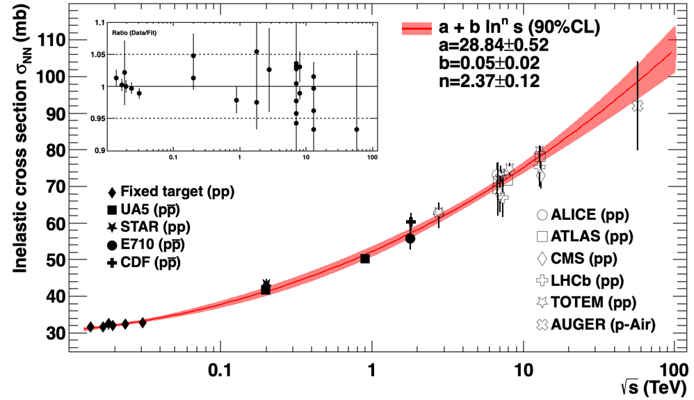
Figure 2: Inelastic pp ($\rm p\bar{p}$) cross sections as a function of c.m. energy measured over $\sqrt{s}\approx 10$ GeV – $100$ TeV fitted to Eq. (6). The inset shows the ratio of the data divided by the value of the fit.

The experimental $\sigma_{\rm NN}$ values are obtained either (i) via the subtraction $\sigma_{\rm pp}=\sigma_{\rm tot}-\sigma_{\rm el}$, where $\sigma_{\rm tot}$ and $\sigma_{\rm el}$ have been accurately measured in dedicated forward Roman pot detectors (TOTEM [59, 60, 61, 62, 63] and ALFA [52, 53, 54]), or (ii) from measurements of inelastic particle production data in the central detectors collected with MB triggers. The latter measurements are less precise than the former, as they require an extrapolation, dominated by diffractive contributions, to forward regions of phase space not covered by the detectors. Many Glauber MC codes, such as glissando [11, 14, 19], use the COMPETE collision-energy parametrization of the NN cross section [65], as provided in the PDG review [43]. However, such a relatively complex multiparameter expression is only required when aiming at a reproduction of the NN cross section data over the full collision energy range experimentally measured, down to $\sqrt{s}\approx 1$ GeV. For the regime of energies relevant at colliders, the $\sqrt{s}$ dependence of the experimental $\sigma_{\rm NN}$ results can be fit to a simpler parametrization, as done in [18],

$$\sigma_{\rm NN}(s)=a+b\,\ln^{n}(s)\,,$$ (6)

resulting in $a=28.84\pm 0.52$, $b=0.0458\pm 0.0167$ and $n=2.374\pm 0.123$ with goodness-of-fit over number of degrees of freedom $\chi^{2}/N_{\rm dof}=0.7$ (and $s$ given in GeV² units). The first row of Table 1 lists the derived $\sigma_{\rm NN}$ values relevant for Glauber calculations at RHIC, LHC, and FCC energies. The value predicted for the top RHIC energy of $\!\sqrt{s_{{}_{\rm NN}}}=0.2$ TeV, $\sigma_{\rm NN}=41.3\pm 1.2$ mb, is consistent with (although, more precise than) the value directly measured by STAR ($\sigma_{\rm NN}=43.82^{+1.39}_{-1.46}$ mb) [49], as well as with the typical $42\pm 3$ mb used so far in the RHIC literature [40]. At the top FCC energy of $\!\sqrt{s_{{}_{\rm NN}}}=100$ TeV, the expected cross section of $\sigma_{\rm NN}=107.5\pm 6.5$ mb is also in agreement with the value $105.1\pm 2.0$ mb derived from the average of various model predictions [66].

Table 1: Top row: Values of the nucleon-nucleon inelastic cross section $\sigma_{\rm NN}$ extracted from Eq. (6) and the data plotted in Fig. 2. Central and bottom rows: Computed values of the pA and AA hadronic cross sections at c.m. energies relevant for collisions at RHIC, LHC, and FCC. The quoted values are for pPb and PbPb collisions, except for the results at 0.2 TeV that correspond to pAu and AuAu collisions.

$\sqrt{s}$ (TeV)	0.2	5.5	8.8	14	39	63	100
$\sigma_{\rm NN}$ (mb)	$41.3\pm 1.2$	$68.3\pm 1.2$	$73.6\pm 1.4$	$79.2\pm 1.9$	$93.0\pm 3.8$	$100.2\pm 5.1$	$107.5\pm 6.5$
$\sigma_{\rm pA}$ (b)	$1.75\pm 0.03$	$2.10\pm 0.03$	$2.13\pm 0.03$	$2.17\pm 0.03$	$2.26\pm 0.04$	$2.30\pm 0.05$	$2.35\pm 0.05$
$\sigma_{\rm AA}$ (b)	$6.84\pm 0.14$	$7.64\pm 0.15$	$7.71\pm 0.16$	$7.78\pm 0.16$	$7.93\pm 0.16$	$8.00\pm 0.17$	$8.07\pm 0.17$

From $\sigma_{\rm NN}$, one can then derive the corresponding values for the pA and AA inelastic cross sections making use of Eq. (2). The $\sigma_{\rm pA}$ and $\sigma_{\rm AB}$ results for the pPb and PbPb (pAu and AuAu for RHIC) systems are listed in the middle and bottom rows of Table 1. The quoted uncertainties account for the propagated $\sigma_{\rm NN}$ uncertainties plus, in quadrature, the resulting uncertainty of independently varying the density parameters by 1 standard deviation. The latter amount to about 2% and 1.5% for PbPb and pPb collisions, respectively, and are dominated by the uncertainty of the neutron skin width. The Glauber calculation gives $\sigma_{\rm PbPb}^{\rm MC}=7.55\pm 0.15$ b at $\!\sqrt{s_{{}_{\rm NN}}}=2.76$ TeV and $\sigma_{\rm pPb}^{\rm MC}=2.09\pm 0.03$ b at $\!\sqrt{s_{{}_{\rm NN}}}=5.02$ TeV, in good agreement with the measured values of $\sigma_{\rm PbPb}=7.7\pm 0.6$ b [67], and $\sigma_{\rm pPb}=2.06\pm 0.08$ b [68] as well as $\sigma_{\rm pPb}=2.10\pm 0.07$ b [69], respectively. At 5.02 TeV, $\sigma_{\rm PbPb}=7.62\pm 0.15$ b for $\sigma_{\rm NN}=67.3\pm 1.2$ mb. The measured ALICE and CMS inelastic pPb and PbPb cross sections provide therefore an inclusive validation of the Glauber model at TeV energies. This fact further justifies the common application of the Glauber approach to derive pp cross section from cosmic-ray proton-air cross section measurements [64].

3 DEVELOPMENTS IN THE INITIAL STATE

In the past fifteen years, there have been numerous developments related to the description of the nucleon and nuclei radial profiles in Glauber models including e.g. the incorporation of various sources of event-by-event fluctuations (particularly relevant for collisions involving light-ions and/or protons), subnucleonic degrees of freedom, neutron skin effects, and deformed light- and heavy-ion distributions. The most important advances on these topics are summarized in this section.

3.1 Proton Transverse Profile

The transverse profile of the proton (or, generically, of the nucleon) is of key importance in many aspects of the Glauber formalism. First, in nuclear collisions, it determines the NN interaction probability, and its realistic description is particularly important to properly describe proton-nucleus results (where intrinsic fluctuations in the proton shape are more relevant than in AA collisions). Second, it is a prime ingredient of MC event generators for pp collisions such as pythia 8 [70] or herwig++ [71] in order to reproduce, through the underlying multiparton interactions (MPIs), the properties of inclusive hadron production both in minimum-bias (MB) collisions —as a sum of the particle production activity from all, central to peripheral, pp collisions— and in the so-called “underlying event” (UE) accompanying hard scatterings at the LHC [72]. Third, the proton transverse distribution is also a basic element in calculations of double- and triple- parton scatterings cross sections in proton and nuclear collisions, where the effective N-parton scattering (NPS) cross section bears a simple geometric interpretation in terms of powers of the inverse of the integral of the pp overlap function over all impact parameters, $\sigma_{\rm eff,\textsc{nps}}=\left[\int{\rm d}^{2}b\,T_{{}_{\rm pp}}^{n}({\bf b})\right]^{-1/(n-1)}$ (with $n=2,3,..,N$ for double-, triple-, $N$-scatterings) [73]. Improving the treatment of pp collisions within a Glauber-like approach based on their impact parameter and underlying parton-parton scatterings has attracted a growing interest in the last years to interpret high-multiplicity pp results where collective (QGP-like) phenomena have been observed in the data [74, 75, 76], a possibility anticipated in [77].

The most simplistic approach used in Glauber models is to consider a fixed proton shape at all colliding energies, disregarding any varying distributions of its parton contents (valence and sea quarks, gluons) and their correlations. The simplest form is a hard-sphere parametrization with uniform density, $\rho(r)={1\over 4/3\;\pi R^{3}}\Theta\left(r-R\right)$ with radius consistent with electron-proton scattering fits giving a root-mean-square radius, $R_{\rm rms}\approx 0.8$ fm [78]. A profile more consistent with the proton charge form factor is given by an exponential, $\rho(r)={1\over 8\pi R^{3}}e^{-r/R}$, reproducing to a large extent the spatial distribution of its valence quarks, with $R=R_{\rm rms}/\sqrt{12}=0.234$ fm. A single Gaussian ansatz, although not very realistic, makes subsequent calculations especially transparent and hence was used in some analytical approaches. A double Gaussian ansatz, $\rho(r)\propto\frac{1-\beta}{a_{1}^{3}}\,e^{-r^{2}/a_{1}^{2}}+\frac{\beta}{a_{2}^{3}}\,e^{-r^{2}/a_{2}^{2}}$, which corresponds to a distribution with a small core region of radius $a_{2}$ containing a fraction $\beta$ of the total matter embedded in a larger region of radius $a_{1}$, is a common choice, available e.g. in the pythia 8 MC generator [79].

In MC event generators for pp collisions, parametrizations of the overlap function as a function of impact parameter, rather than the individual radial density of each colliding proton, are usually used. In pythia 8, the pp overlap is parametrized as

$$T_{{}_{\rm pp}}({\bf b})=\frac{m}{2\pi r^{2}_{p}\,\Gamma(2/m)}\exp{[-(b/r_{p})^{m}]}\,,$$ (7)

normalized to one, $\int{\rm d}^{2}b\,T_{{}_{\rm pp}}({\bf b})=1$, where $r_{p}$ is a characteristic “radius” of the proton, $\Gamma$ is the gamma function, and the exponent $m$ varies between a more Gaussian-like ($m\approx 2$) to a more peaked exponential-like ($m\approx 1$) distribution. The popular pythia 8 “Monash” parameter settings (tune) uses $m=1.85$ [80]. In the hijing [10] and herwig++ [71] generators, the pp overlap is approximated by the Fourier transform of the proton e.m. form factor as

$$T_{{}_{\rm pp}}({\bf b})=\frac{\mu^{2}}{96\pi}\,(\mu\,b)^{3}\,K_{3}(\mu\,b)\,,$$ (8)

where $\mu\propto 1/r_{p}$ is a free parameter, and $K_{3}$ is the modified Bessel function of the third kind. In hijing, $\mu=3.9/\!\sqrt{\sigma_{\rm NN}/2\pi}$ is used to describe the dependence of $\mu$ on the effective size of the proton.

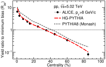
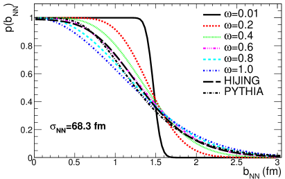
Figure 3: Left: Yield of high-$p_{\rm T}$ charged particles in multiplicity classes measured in pp collisions at $\sqrt{s}=5.02$ TeV normalized to their MB yield [81], compared to hg-pythia and pythia 8 predictions. Right: Nucleon-nucleon collision probability distribution using Eq. (9) for various $\omega$ values in NN collisions at $\sqrt{s}=5.02$ TeV, compared to the result from the hijing and pythia 8 (Monash) overlap profiles.

The importance of properly taking into account the proton transverse profile in pp collisions at LHC energies is illustrated in Fig. 3 (left) where the high-$p_{\rm T}$ hadron yield (normalized to its impact-parameter-integrated value) as a function of centrality measured by the ALICE experiment at $\sqrt{s}=5.02$ TeV, is shown. The multiplicity classes are obtained by ordering events according to the charged-particle response in the ALICE VZERO scintillators ($2.8<\eta<5.1$ and $-1.7<\eta<-3.7$) for events with at least one charged particle produced at midrapidity ($|\eta|<1$). Central (peripheral) pp collisions feature about ten times larger (smaller) yields than MB collisions, consistent with the expectation from the MPI picture [82]. The centrality dependence of the yields is well reproduced by hg-pythia [83] and (slightly less well) by pythia 8 (Monash tune), where the former basically corresponds to pythia with the proton overlap profile given by Eq. (8).

The above discussion highlights the importance in MCG simulations of the choice of the NN collision profile, whereby two nucleons collide if their impact parameter is less than a given distance parameter $D\approx\!\sqrt{\sigma_{\rm NN}/\pi}$. The simplest collision profiles used are the hard sphere (HS), $p(b_{{}_{\rm NN}})=\Theta(\sqrt{\!\sqrt{s_{{}_{\rm NN}}}}-b_{{}_{\rm NN}})$ (also called “black disk”), and Gaussian, $p(b)=\exp{(-a\,b^{2}/D^{2})}$, with $a$ fitted to reproduce the $\sigma_{\rm NN}$ inelastic cross section (e.g. $a=0.92$ at RHIC energies) [14], although more involved probabilistic ways to model the NN interaction have been known for a long time [84]. At LHC energies, a modification of the collision profile proposed by Refs. [85, 14] uses a parametrization based on the Euler $\Gamma(z)$ and incomplete $\Gamma(\alpha,z)$ gamma functions

$$p(b_{{}_{\rm NN}})=G\;\Gamma\left(1/\omega,\frac{G\,b_{{}_{\rm NN}}^{2}}{D^{2}\omega}\right)\bigg{/}\Gamma(1/\omega)\,,$$ (9)

where $\omega$ interpolates between the HS ($\omega\to 0$) and Gaussian ($\omega\to 1$) cases. The choice $(G,\omega)=(1,0.4)$ reproduces the measured $\sigma_{\rm NN}\approx 73$ mb and $\sigma_{\rm pp,el}\approx 25$ mb LHC results. Figure 3 (right) compares NN collision profiles for varying values of the $\omega$ parameter and with the pythia 8 Monash and hijing choices for pp collisions at $\!\sqrt{s_{{}_{\rm NN}}}=5.02$ TeV. The two latter are obtained via $p(b_{{}_{\rm NN}})=1-\rm{e}^{-kT_{{}_{\rm pp}}(b_{{}_{\rm NN}})}$ so that $2\pi\int p(b_{{}_{\rm NN}})\;{\rm d}b_{{}_{\rm NN}}$ gives $\sigma_{\rm NN}$, as commonly done for profile functions. One can see that the pythia 8 Monash and hijing profiles correspond approximately to the $\omega=0.6$ choice in Eq. (9).

An extension of the nuclear Glauber approach to pp collisions at the parton-level was described in Ref. [77] where, by analogy to the nuclear case, the thickness function of a proton with $N_{g}$ partons is written as $T_{p}(x,\vary)=N_{g}\int{{\rm d}}z\;\rho(x,\vary;z)$, normalized to $\int{\rm d}^{2}{\rm b}\,T_{p}(b)=N_{g}$. The overlap function of a pp collision at $b$ can be obtained as a convolution over the corresponding thickness functions of each proton normalised to $\int{\rm d}^{2}{\rm b}\,T_{{}_{\rm pp}}(b)=N_{g}^{2}$. From the partonic cross section $\sigma_{gg}$, one can then define the number of binary parton-parton collisions in a pp collision at impact parameter $b$: $N_{\rm coll,gg}(b)=\sigma_{gg}\,T_{{}_{\rm pp}}(b)$. From this, the probability of an inelastic parton-parton interaction at impact parameter $b$ can be defined as $P_{gg}^{\rm inel}(b)=1-e^{-\sigma_{gg}\,T_{{}_{\rm pp}}(b)}\,$, where the value of $\sigma_{gg}$ is obtained by requiring that the proton-proton inelastic cross section obtained from the pp overlap function, $\int{\rm d}^{2}\,{\rm b}\;\left(1-e^{-\sigma_{gg}\,T_{{}_{\rm pp}}(b)}\right)=\sigma_{\rm pp}$, matches the $\sigma_{\rm pp}^{\rm inel}\approx 40$–80 mb values measured at RHIC and LHC energies (Table 1). Values of $\sigma_{gg}\approx 6$ mb are used that are consistent with a simplistic perturbative gluon-gluon cross-section of $\sigma_{gg}=K\cdot(9/2)\,\pi\,\alpha^{2}_{s}/p_{\rm T}^{2}$ for $\alpha_{s}\approx$ 0.5 at a $p_{\rm T}$-cutoff of the order 1 GeV, where $K\approx 2$ is a factor accounting for higher-order pQCD corrections. The final particle multiplicity density in a pp collision follows the same impact-parameter-dependence as that of the number of binary parton-parton collisions, $N_{coll,gg}(b)$, and the average multiplicity in a pp collision, integrated over all impact-parameters, is $\frac{dN_{\rm MB}}{d\eta}={dN_{0}\over d\eta}\int{\rm d}^{2}{\rm b}\;N_{\rm coll,gg}(b)\,P_{gg}^{\rm inel}(b)\;$, with the absolute normalisation $dN_{0}/{\rm d}\eta$ chosen so as to reproduce the MB pp multiplicity of $dN_{\rm MB}/{\rm d}\eta\approx$ 10 measured at midrapidity at LHC energies [86].

Other extensions of the nuclear MCG simulations to account for subnucleonic degrees of freedom, such as e.g. three constituent valence quarks, exist [87, 16, 17, 88, 19]. The number of partonic constituents and the way to distribute them in pA and AA collisions —between the two extremes of bound to individual nucleons (according e.g. to a radially exponential nucleon form factor) or freely-distributed over the nucleus (following a global 2pF profile)— must be chosen so as to reproduce basic experimental quantities (inelastic cross sections $\sigma_{\rm NN}$, $\sigma_{\rm pA}$, $\sigma_{\rm AA}$, overall particle multiplicities), and have a different impact on the event ellipticity and triangularity. Accounting for subnucleonic degrees of freedom is particularly important to generate realistic initial conditions for small QGP systems at the LHC, as discussed in Sec. 4.3.

3.2 Fluctuations and Correlations

Traditionally, Glauber studies have just dealt with average nucleon and nuclear transverse densities, but in the last decade more and more studies have incorporated event-by-event shape fluctuations generated by various underlying mechanisms. Such developments have been largely motivated by an increasing number of experimental observations that pointed to the need of enhanced eccentricities fluctuations in order to explain e.g. the large azimuthal harmonics —direct [89], elliptic [90], and triangular [30, 31, 27, 32, 33, 34] flows— observed in the data.

There are two obvious sources of quantum fluctuations in MCG simulations: fluctuations in the positions of nucleons within the nucleus, and fluctuations at the subnucleonic level. The former are in principle properly accounted for by conventional MCG simulations [91], and we thus focus mostly on the latter. Nucleons are composite quantum-mechanical systems with varying spatial and momentum configurations of their internal quark and gluon constituents, and the overall transverse area occupied by their color fields changes event by event, a phenomenon often referred to as color fluctuations (CFs) [92, 93, 94]. Such fluctuations can lead to potentially large changes of the effective collision-by-collision nucleon transverse size that are often not accounted for in MCG codes, notably when the NN interaction is approximated by a simple “black disk” approach (see above). Whereas such CFs tend to average out in central AA collisions, they are of importance for pp and pA collisions. The CFs have been evaluated theoretically in terms of the cross section for inelastic diffractive processes in pN scattering, often referred to as “Glauber–Gribov” approach [95], generalized to the nuclear case [92], and have been phenomenologically encoded into an event-by-event variation of $\sigma_{\rm NN}$ given by a probability distribution of the form

$$P_{\sigma}(\sigma_{\rm NN})=C\frac{\sigma_{\rm NN}}{\sigma_{\rm NN}+\sigma_{0}}\exp^{-\left(\frac{\sigma_{\rm NN}-\sigma_{0}}{\sigma_{0}\,\Omega}\right)^{2}}\,,$$ (10)

where $\sigma_{0}$ denotes the mean $\sigma_{\rm NN}$ value, and $\Omega$ its width. The normalization $C$ is computed from the provided input (mean $\sigma_{\rm NN}$ and $\Omega$) requiring $\int\sigma P{\rm d}\sigma/\int P{\rm d}\sigma=\sigma_{0}$, with the dispersion given by the ratio of inelastic diffraction over elastic cross section at $t=0$ (zero momentum exchange). Variations of the nucleon interaction strength naturally lead to increased fluctuations in the number of participant nucleons and binary nucleon collisions, e.g. longer tails in the $N_{\rm part}$ and $N_{\rm coll}$ distributions, compared to the pure eikonal picture. Example distributions for pPb collisions at the LHC with varying width values $\Omega=0,0.5,1$, are shown in Fig. 4 (left).

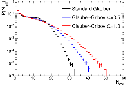
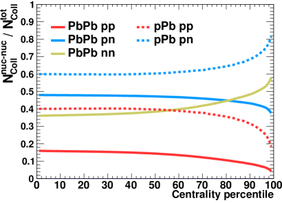
Figure 4: Left: Comparison of the $N_{\rm coll}$ distributions for pPb collisions at the LHC with different values of the Glauber–Gribov corrections given by $\Omega=0,0.5,1$ in Eq. (10). Right: Average fraction of pp, pn, and nn collisions for PbPb (solid curves) and pPb (dashed curves) obtained by incorporating a neutron skin in the Pb density profile as described in the text. Both distributions are obtained with TGlauberMC.

Microscopic refinements in the MCG treatment of fluctuations from diffractive scatterings in pA collisions have been discussed in Ref. [96], which proposed a log-normal parametrization instead of Eq. (10). In addition, CFs explain the existence of partonic configurations of the nucleon with smaller-than-average interaction strength that lead to observable differences in the centrality dependence of single jet production in dAu and pA collisions observed in the data at RHIC and the LHC [97, 98]. Such events are characterized by a configuration in which a large fraction of the proton momentum is carried by a single parton, e.g. $x\gtrsim 0.1$, that is more spatially compact than the average, and their interaction strength is thereby reduced with respect to the eikonal limit [99]. The standard MCG models underestimate the associated number of “peripheral” events with low hadronic activity, while they overestimate the “central” ones with a large hadronic activity, although inclusive jet production rates remain unmodified.

Most Glauber-like calculations are based upon the pure eikonal approximation and disregard higher-order terms of the expansion Eq. (1) that account for short-range two-, and three-nucleon correlations (many-nucleon correlations are further suppressed). The impact of realistically correlated NN configurations (centrally correlated nucleon configurations, two-body full correlations, three-body chains) on the medium eccentricity has been studied in Ref. [84], where it was found that their combined effects cancel out and bring the results close to the no-correlations case. The impact of NN correlations and their interplay with diffractive effects on $N_{\rm coll}$  have been estimated in Ref. [100]. This latter work found that such correlations slightly decrease (respectively, increase) by a few percent the $N_{\rm coll}$ values (resp., $\sigma_{\rm pA}$ and $\sigma_{\rm AA}$) compared to the pure Glauber results, but that such effects are cancelled when taking into account diffractive (aka. “Gribov inelastic shadowing”) corrections that act in the opposite direction. The number of nucleons that are diffractively excited in the multiple collisions but revert back to their ground state before the scattering process is completed, both increases the nuclear transparency (i.e. reduce the nuclear cross section) and reduces the $N_{\rm coll}$ results back to the values obtained with the conventional Glauber codes. Another possible source of correlations in MCG simulations is due to the recentering procedure [18] by which the MC setup of the initial nuclear profile without nucleons overlaps is done in such a way so that the c.m. of each nucleus is fixed at a given location in each event. Those correlations are found to be small, in particular for large nuclei [91]. Correlations at the parton level due to the interference of same-color gluons from different nucleons, evaluated with the dipsy generator [101] based on a BFKL resummation of small-$x$ dipoles [102], were found to result only in few percent effects for pA collisions with heavy nuclei.

3.3 Neutron Skin and Isospin Effects

The transverse profile of nucleons inside a nucleus is commonly described by a single 2pF distribution. An ansatz, based on electromagnetically probing the charge distribution (protons) of nuclei, that is however not supported by measurements with strongly-interacting probes that prefer instead two nonidentical distributions for protons and neutrons [103], in particular at the surface of heavy stable neutron-rich nuclei, such as ²⁰⁸Pb with a neutron excess of $N/Z\approx 1.5$ [104, 105]. These differences appear because protons around the center of the nucleus feel their common electromagnetic repulsion from all directions resulting in an electrostatic equilibrium at a constant charge density, but the outermost protons at $r\!\gtrsim\!6$ fm, where the nucleon density begins to drop, need additional “skin” or “halo” neutrons in the periphery to counteract the outward Coulomb repulsion and maintain a sufficient nuclear surface tension.

The nominal heavy-ion species at the LHC is ²⁰⁸Pb, the heaviest stable doubly magic nucleus and one of the most intensively studied isotopes. While the average charge radius of ²⁰⁸Pb is known to within $\pm 0.001$ fm [21, 106], past estimates placed the uncertainty in the neutron radius at about $\pm 0.2$ fm [107]. Neutron point density parameters of $R_{\rm n}=6.67\pm 0.03$ (stat.) fm and $a_{\rm n}=0.55\pm 0.01$ (stat.)${}^{+0.02}_{-0.03}$ (syst.) fm have been measured by the Crystal Ball collaboration via coherent pion photoproduction [105], while the CERN LEAR experiment reports comparable values of $R_{\rm n}=6.684\pm 0.02$ (stat.) fm and $a_{\rm n}=0.571$ fm derived from antiproton-nucleus interactions coupled with radiochemistry techniques [104]. These data favor a peripheral neutron distribution in the form of a neutron “skin” rather than a neutron “halo”, i.e. the neutron distribution is slightly broader than the proton one because of its larger diffusivity ($a_{\rm n}-a_{\rm p}\approx 0.1$ fm), but has the same half-radius as the proton distribution ($R_{\rm p}\approx R_{\rm n}\approx 6.7$ fm). The combined point density distribution for proton and neutrons has been implemented in recent MCG simulations [18] via the weighted sum of the individual 2pF distributions. For peripheral PbPb collisions, this results in a maximum $\sim$4% increase in $N_{\rm coll}$ and approximately half this percentage for pPb collisions, largely driven by the increase of the central radius in the D2pF compared to the 2pF parametrization. If one focuses instead on the transverse distribution of the underlying $d$ quarks, the dominant flavor in neutrons, larger effects are expected for precise phenomenological studies of isospin-dependent gauge boson ($\gamma$, W^±, and Z) cross sections in nuclear compared to proton collisions [108, 109, 110, 111]. Figure 4 (right) shows the average fraction of pp, pn, and nn scatterings for PbPb and pPb collisions versus centrality illustrating the increasing relevance of the neutron density for peripheral collisions.

3.4 Light and Heavy Deformed Nuclei

For a number of years, the RHIC machine has been providing collisions with a variety ions beyond the nominal gold nucleus, ranging from the lightest species such as deuteron and helium-3 [112] to the heaviest ones such as uranium [113], as a means to study the system size dependence of various QGP-related signals. As aforementioned, for spherical nuclei, the probability density distribution in MCG models is sampled from the underlying 2pF or D2pF radial probability functions, and taken to be uniform in azimuthal and polar angles, but light species such as the deuteron (²H), tritium (³H), helium-3 (³He), helium-4 (⁴He), carbon (¹²C), oxygen (¹⁶O), and sulfur (³²S), have dedicated parametrizations of their transverse profiles. For deuteron, the Hulthén form $\rho(r^{\prime})=\rho_{0}\left(\frac{e^{-ar^{\prime}}-e^{-br^{\prime}}}{r^{\prime}}\right)^{2}$, with $a=0.228$ fm^-1 and $b=1.177$ fm^-1, and $r^{\prime}=2r$ denoting the distance between the proton and neutron, is often employed [114, 115, 116]. For ³H and ³He nuclei, configurations are computed from Green’s function MC calculations using the AV18/UIX Hamiltonian, which correctly sample the position of the three nucleons, including their correlations [117]. Similarly, results of wavefunction-based calculations are available for helium-4, carbon, and oxygen [118]. For slightly deformed nuclei, such as e.g. sulfur, the Fermi distribution is modified with an extra parameter $w$ and a Gaussian term, $\rho(r)=\rho_{0}\frac{1+w(r/R)^{2}}{1+\exp(\frac{r^{2}-R^{2}}{a^{2}})}$. Details on all relevant parametrizations can be found in App. A and in Refs. [15, 118, 119].

The description of the transverse profile of heavy deformed nuclei starts off with the 2pF expressions modified with an expansion of $R$ in spherical harmonics, $\rho(r)=\rho_{0}\left(1+\exp\frac{\left[r-R(1+\beta_{2}Y_{20}+\beta_{4}Y_{40})\right]}{a}\right)^{-1}$, with $Y_{20}=\sqrt{\frac{5}{16\pi}}(3\cos^{2}(\theta)-1)$, $Y_{40}=\frac{3}{16\sqrt{\pi}}(35\cos^{4}(\theta)-30\cos^{2}(\theta)+3)$, and deformation parameters $\beta_{2}$ (quadrupole) and $\beta_{4}$ (hexadecapole) [21]. The higher harmonic eccentricities ($\epsilon_{n}$) of the initial QGP produced in collisions of deformed nuclei, such as U, are particularly sensitive to the parametrization of their profiles. A proper description of collisions of heavy deformed nuclei requires also accounting for their relative, tip-on-tip and side-on-side, orientations. Tip-on-tip collisions produce a smaller elliptic flow but larger particle multiplicities (entropy densities), whereas on the contrary, side-on-side collisions generate a larger elliptic flow but a smaller multiplicity. The scaling of $v_{2,3}$ flows with multiplicity in ultracentral collisions (0–1% centrality percentile) in small and deformed systems produced in UU, dAu, ⁹BeAu, ⁹Be⁹Be, ³He³He, and ³HeAu collisions at RHIC energies, including or not fluctuations from subnucleonic degrees of freedom, has been theoretically studied in [120, 121]. This work indicates that such collisions can help discriminate between different initial entropy densities of the QGP medium formed at RHIC and LHC [122, 123]. Implications for the extraction of QGP transport properties such as its viscosity, are further developed in Sec. 4.3.

4 PHENOMENOLOGICAL APPLICATIONS

The Glauber model has many important phenomenological uses in nuclear collisions at colliders. We consider three typical cases here. First, in the definition of the baseline scalings for comparing hard-scattering cross sections in pp, pA, and AA collisions. Second, as an underlying framework for MC event generators used in high-energy heavy-ion and cosmic-ray physics. Third, to provide realistic initial-state conditions of the created QGP for subsequent spacetime evolution in hydrodynamics codes. We succinctly review below the basic ideas and latest progress in these three areas.

4.1 Binary Scaling for Hard Scatterings

One of the most extended uses of the Glauber model is to properly normalize the fractional cross sections or yields for the production of a given particle in hard-scattering processes (i.e. partonic processes characterized by mass and/or $p_{\rm T}$ scales above a few GeV) in AA and pA collisions, to be able to compare them to those expected in the simpler pp collisions where no QGP formation is, in principle, expected. For pQCD observables that do not suffer any final-state effects, the assumption of binary scaling allows the extraction of modifications of the nuclear parton distribution functions (PDFs) compared to the free proton ones.

It is informative to recall the basic scaling rules for perturbative scatterings in nuclear collisions [124, 125]. For a given hard process A$+$B$\,\to h+X$, from the generic Eq. (2) for the inclusive AA cross section, one obtains the following relationship between pp and nuclear collisions

$$\sigma_{\rm AB}^{\rm hard}=\int d^{2}b\;\sigma_{\rm NN}^{\rm hard}\;T_{{}_{\rm AB}}(b)\,,\;\mbox{and, therefore, }\;\sigma_{\rm AB,MB}^{\rm hard}=\;A\cdot B\cdot\sigma_{\rm NN}^{\rm hard}\;,$$ (11)

where the second expression for the inclusive hard cross section is obtained integrating the former over the impact parameter. The associated minimum-bias invariant yield per nuclear collision, $N^{\rm hard}_{\mbox{\scriptsize{\rm AB}}}=\sigma^{\rm hard}_{\mbox{\scriptsize{\rm AB}}}/\sigma_{\rm AB}$, for a given hard process in an AB collision compared to that of a pp collision is $\langle N_{\scriptsize{\rm AB}}^{\rm hard}\rangle_{\scriptsize{\rm MB}}=\frac{A\cdot B}{\sigma_{\rm AB}}\cdot\sigma_{\rm NN}^{\rm hard}\;$, where $\sigma_{\rm AB}$ is the inclusive inelastic AB cross section given by Eq. (2). The average nuclear overlap function at impact parameter $b$ for minimum-bias collisions is

$$\langle T_{{}_{\rm AB}}(b)\rangle_{\scriptsize{\rm MB}}\equiv\frac{\int{\rm d}^{2}b\,T_{{}_{\rm AB}}(b)}{\int{\rm d}^{2}b}\;=\frac{A\cdot B}{\pi(R_{A}+R_{B})^{2}}=\frac{A\cdot B}{\sigma_{\rm AB}}\;.$$ (12)

The corresponding expressions for a given impact parameter $b$ can be obtained by multiplying each nucleon in nucleus A with the density along the $z$ direction in nucleus B, integrated over nucleons in nucleus A, i.e.

$$N_{\scriptsize{\rm AB}}^{\rm hard}(b)=\sigma_{\rm NN}^{\rm hard}\int{\rm d}^{2}\mathbf{s}\int\rho_{A}({\mathbf{s},z^{\prime}})\int{{\rm d}}z^{\prime\prime}{{\rm d}}z^{\prime}\,\rho_{B}(|\mathbf{b}-\mathbf{s}|,z^{\prime\prime})\;\equiv\;\sigma_{\rm NN}^{\rm hard}\cdot T_{{}_{\rm AB}}(b)\;.$$ (13)

Similarly, one obtains a useful expression for the probability of an inelastic NN collision or, equivalently, for the number of binary inelastic collisions, $N_{\rm coll}$, in a nucleus-nucleus collision at impact parameter $b$:

$$N_{\rm coll}(b)\;=\;\sigma_{\rm NN}\cdot T_{{}_{\rm AB}}(b)\,.$$ (14)

From this last expression, one can see that the nuclear overlap function, $T_{{}_{\rm AB}}(b)=N_{\rm coll}(b)/\sigma_{\rm NN}$ [mb^-1], can be thought of as the hard-scattering integrated luminosity (i.e. the number of hard collisions per unit of cross section) per AB collision at a given impact parameter.

The expressions above allow writing the standard binary (or point-like) collision scaling formula that relates the hard-scattering yields in nuclear and proton collisions as $N_{AB}(b)=N_{\rm coll}(b)\cdot N_{pp}$. The nuclear modification factor for hard-scattering processes is thereby defined as the ratio of AA over scaled pp cross sections and/or yields (here, differential in $p_{\rm T}$ and $\eta$) as

$$R_{\rm AB}(p_{\rm T},\eta)=\frac{d\sigma_{\rm AB}/dp_{\rm T}d\eta}{(A\cdot B)\;d\sigma_{\rm pp}/d{\rm d}p_{\rm T}\eta}\,,$$ (15)

for minimum-bias collisions, and dependent on $b$ as

$$R_{\rm AB}(p_{\rm T},\eta;b)=\frac{dN_{AB}(b)/dp_{\rm T}d\eta}{T_{{}_{\rm AB}}(b)\;d\sigma_{\rm pp}/dp_{\rm T}d\eta}=\frac{dN_{AB}(b)/dp_{\rm T}d\eta}{N_{\rm coll}(b)\;dN_{pp}/d{\rm d}p_{\rm T}\eta}\;.$$ (16)

In the absence of any final- and/or initial-state effects, one expects $R_{\rm AB}=1$ for any hard-scattering process. The equality of Eq. (15) or (16) to unity, modulo few percent nuclear PDF effects (see below), for colorless hard probes that do not suffer final-state interactions in the produced QGP was confirmed previously in heavy-ion collisions at SPS and RHIC as well as, in the last years, at LHC energies, and constitutes a validation of the basic assumptions of the Glauber model itself. Prominent examples include the production yields of photons [126, 127, 128, 129], and W and Z bosons [130, 131, 132, 133, 134, 135, 136, 137] in pPb and PbPb collisions.

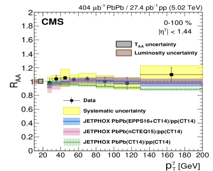
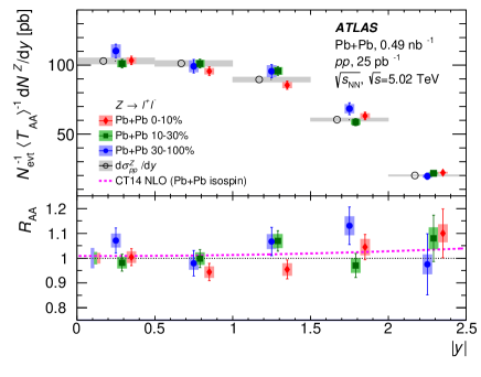
Figure 5: Nuclear modification factors $R_{\rm AA}$ measured for isolated photons as a function of $p_{\rm T}^{\gamma}$ (left) [129] and Z bosons as a function of rapidity (right) [135] in PbPb collisions at the LHC, compared to pQCD NLO calculations with nuclear PDFs.

Figure 5 shows the $R_{\rm AA}$ values measured for isolated photons [129] and Z bosons [135] as functions of $p_{\rm T}^{\gamma}$ and rapidity $|y^{Z}|$, respectively, in PbPb collisions at the LHC. Both ratios are around unity with small variations due to nuclear PDF modifications related either to the increased number of $d$-quarks in the Pb nucleus compared to protons (isospin effects) and/or to few percent (anti)shadowing effects at the large virtualities ($Q^{2}\approx p_{\rm T}^{\gamma},m_{\mathrm{Z}}$) probed in the underlying partonic scatterings. Under the key assumption of binary scaling, the precision of the PbPb data (a few percent experimental uncertainties in the case of electroweak gauge bosons) allows the derivation of the EPPS16 [138], nCTEQ15 [139], and nNNPDF2.0 [140] nuclear PDFs at next-to-leading order (NLO), or more recently also next-to-next-to-leading order (NNLO) [141] accuracy, through global fits combining nuclear deep-inelastic scattering (DIS) and LHC electroweak boson data. Precision electroweak boson measurements in PbPb collisions can also be used to derive a data-driven normalization, in principle independent of the Glauber model, for cross section measurements in PbPb collisions, as explored in [142].

4.2 Heavy-Ion Monte Carlo Event Generators

All existing generic event generators of ultrarelativistic pA and AA collisions —such as hijing 1.0 [10] and 2.0 [143], epos-LHC [144], ampt [145], qgsjet-II [146], dpmjet-III [147], as well as the more recent pythia 8-based [148] angantayr [149] code— internally rely on a Glauber picture to model the early stage of the collision through the proper computation of the number of inelastic subcollisions for any reaction centrality. The main differences among models arise from their treatment of the underlying (semi)hard scatterings: minijets in the case of the hijing, angantayr, and ampt codes mostly used in collider physics; and Regge–Gribov “cut pomerons” (aka. parton ladders, giving rise to one or two strings spanned between two colliding nucleons, or between a nucleon and another pomeron) in the case of the epos-LHC, qgsjet-II, and dpmjet-III codes that are mostly used in cosmic-ray physics [150]. The final hadronization of partons or strings is carried out via (variations of) the Lund fragmentation model [151] in all generators.

The hijing generator relies on the eikonal approach to determine the number of inelastic subcollisions of two types: soft NN collisions treated as in the Fritiof approach [152], and (multiple) hard parton-parton collisions treated perturbatively as in pythia. The transverse momentum cutoff $p_{\rm T,0}\approx 2$ GeV that separates hard from soft scatterings increases slowly with collision energy (logarithmically, similar to the inelastic cross section Eq. (6) evolution), so that the total number of minijets per unit transverse area satisfies $p_{\rm T,0}^{2}/\pi>T_{{}_{\rm AA}}(b)\,\sigma_{\rm hard}/(\pi R_{A}^{2})$, where $\sigma_{\rm hard}$ is the pQCD cross section for $2\rightarrow 2$ parton scatterings, and $T_{{}_{\rm AA}}(b)$ is the overlap function of the AA collision. The probability for an inelastic NN collision is given by ${\rm d}\sigma_{\rm NN}=2\pi\,b_{{}_{\rm NN}}\,{\rm d}b_{{}_{\rm NN}}\,\left[1-e^{-\left(\sigma_{\rm soft}+\sigma_{\rm hard}\right)\,T_{{}_{\rm NN}}(b_{{}_{\rm NN}})}\right]$ with $T_{{}_{\rm NN}}(b_{{}_{\rm NN}})$ given by Eq. (8). At $\!\sqrt{s_{{}_{\rm NN}}}=0.2$ and 5.02 TeV, $\sigma_{\rm hard}=11.7$ and $124.3$ mb, respectively, and the associated number of MPI per NN interaction is distributed as $P(N^{\rm hard}_{\rm NN})\propto e^{-\langle N^{\rm hard}_{\rm NN}\rangle}$, around the average number of hard scatterings determined by $b_{{}_{\rm NN}}$ and given by $\langle N^{\rm hard}_{\rm NN}\rangle=\sigma_{\rm hard}\,T_{{}_{\rm NN}}(b_{{}_{\rm NN}})$. The average number of hard collisions per NN collision increases from $\langle N^{\rm hard}_{\rm NN}\rangle=0.28$ to 1.77 between $\!\sqrt{s_{{}_{\rm NN}}}=0.2$ and 5.02 TeV. The total number of hard scatterings for an AA collision is then obtained by summing over all NN collisions in the MC Glauber, i.e. $N_{\rm hard}=\sum_{i=1}^{N_{\rm coll}}\left(N^{\rm hard}_{\rm NN}\right)_{i}$.

The ampt code uses directly the Glauber initial conditions generated by hijing as input for its parton cascade evolution. The most recent heavy-ion event generator is angantayr, which follows a Glauber approach similar to that of hijing but further takes into account Glauber–Gribov corrections, by dividing up each inelastic sub-collision as either single-, double-diffractive, or absorptive (i.e. nondiffractive), and with CF effects implemented through a model with fluctuating nucleon radii resulting in a fluctuating NN cross section inspired by the approach of Ref. [93].

At variance with other generators, epos-LHC keeps track of how many times a given nucleon interacts with nucleons from the other nucleus, and separates them event-by-event into the “core” (nucleons that collided more than once) and “corona” (nucleons that interacted exactly once). Event-by-event, a fraction of the string segments that do not overlap (corona) fragment into hadrons normally, following the Lund string model, whereas the other clusters with large density of strings, are used to create a (QGP-like) core that can flow and hadronize collectively. Such a two-component core-corona medium leads to a consistent reproduction of the particle-multiplicity dependence of a number of observables ($\left<p_{\rm T}\right>$, ratio of different hadron yields, etc.) in pp, pA, and AA collisions [144]. The subsequent collective expansion of the medium, defined by the initial core particle density, is taken care of by relativistic hydrodynamics equations.

Apart from the hadronic MC event generators mentioned above, generators of ultraperipheral (photon-induced) nuclear collisions, such as starlight [153] and superchic 3 [154] also employ a Glauber approach to determine the non-hadronic overlap probability needed to compute the cross sections of purely exclusive final states. In starlight, the probability of having no hadronic interactions is given by $P_{\rm no.had}(b)=\mathrm{e}^{-\sigma_{\rm NN}T_{{}_{\rm A}}(b)}$, where $T_{{}_{\rm A}}(b)$ is the nuclear thickness function. For large nuclei, applying this probability function is roughly equivalent to imposing a $b>R_{\rm A}$ condition on their photon flux. This probability is also used when the photon is emitted by the proton, leading to an effective $\gamma$ flux in pA collisions considerably smaller than if it was calculated directly from the e.m. proton form factor.

4.3 Initial Conditions for Hydrodynamic QGP Evolution Calculations

The strongly-interacting medium created in AA collisions at the LHC is a dynamical system that expands, cools down, and transforms into a hadron gas at times around $\tau=10$–15 fm/c. Under such conditions, the extraction of QGP properties can only be accomplished by comparing the experimental measurements of the hadronic final-state to theoretical predictions that include a model of the full spacetime evolution of the heavy-ion collision process [155]. The current state-of-the-art for the QGP evolution is given by 3-D viscous relativistic fluid dynamics calculations [24, 27, 156, 157, 29] —where the plasma thermodynamic properties evolve according to the lattice QCD EoS [2, 3] with nonideal corrections encoded in the medium shear viscosity $\upeta$— matched to a hadron transport cascade (often, the UrQMD code [158]) once the energy density drops below $\upepsilon_{\rm c}$. The largest source of uncertainty in the extraction of medium properties from data-theory comparisons lies in the description of the initial state of the QGP [26], a topic that is discussed next.

Hydrodynamic models start their evolution at $\tau_{0}$ from a given input entropy (or energy) density in the transverse plane $s_{0}(\vec{r}_{\perp})$. In principle, such initial conditions (ICs) should be consistently derived by solving the non-equilibrium evolution of the matter created in the first parton-parton interactions, but achieving thermalization of the interacting fields in ultrashort $\mathscr{O}(1\,{\rm fm})$ time-scales remains a difficult theoretical problem in heavy-ion physics [159]. Therefore, one assumes that the produced matter has (pre)equilibrated, and the ICs are usually given either by

(i) the number density of produced gluons after the primary collisions, via $s_{0}(\vec{r}_{\perp})\propto dN_{g}/(\tau_{0}{\rm d}^{2}r_{\perp}{\rm d}\eta)$, derived analytically e.g. in models such as MC-KLN [160, 161] and IP-Glasma [162, 163] based on the Color-Glass Condensate (CGC) effective theory for parton saturation in heavy-ion collisions [164], or by pQCD NLO calculations with ad hoc parton saturation such as EKRT [165, 166];

(ii) Glauber MC profiles such as those shown in Fig. 1 obtained with the ansatz given by Eq. (4) with $\alpha$ adjusted to match the observed multiplicity distributions, or similarly generated with one of the MC event simulations (hijing, epos, etc.) discussed in Sec. 4.2 .

The corresponding local deposition of the entropy density from the underlying (parton or nucleon) collisions, and thereby the transverse area and azimuthal anisotropies of the produced medium, are then model dependent. The TRENTo approach [167] has parametrized all different approaches with a generic function of the participant target and projectile thickness functions $T_{\rm A,B}^{\rm part}$, as

$$s\propto\left(\frac{T_{{}_{\rm A}}^{\rm part}+T_{{}_{\rm B}}^{\rm part}}{2}\right)^{1/p}\,,$$ (17)

with a continuous parameter $p$ that effectively interpolates among different entropy deposition schemes. For ${p=(1,0,-1)}$, this generalized mean reduces to arithmetic $(T_{{}_{\rm A}}^{\rm part}+T_{{}_{\rm B}}^{\rm part})/2$, geometric $\sqrt{\smash[b]{T_{{}_{\rm A}}^{\rm part}T_{{}_{\rm B}}^{\rm part}}}$, and harmonic $(2\,T_{{}_{\rm A}}^{\rm part}T_{{}_{\rm B}}^{\rm part}/(T_{{}_{\rm A}}^{\rm part}+T_{{}_{\rm B}}^{\rm part}))$ means, while for ${p\rightarrow\pm\infty}$ it asymptotes to maximum $s\propto\max(T_{{}_{\rm A}}^{\rm part},T_{{}_{\rm B}}^{\rm part})$ and minimum $s\propto\min(T_{{}_{\rm A}}^{\rm part},T_{{}_{\rm B}}^{\rm part})$ functions. The generalized Eq. (17) maps different model calculations for suitable values of the parameter $p$. The Glauber wounded nucleon model (WNM), with $s\propto T_{{}_{\rm A}}^{\rm part}+T_{{}_{\rm B}}^{\rm part}$, is equivalent to the generalized mean ansatz with $p=1$. The IP-Glasma approach —which combines CGC effects of the incoming gluon distributions, where the gluon thickness function $T_{g}(b)$ is a Gaussian function of the impact parameter (from the center of the probed nucleon) with a width constrained by HERA DIS data [168], with an event-by-event classical Yang–Mills evolution of the produced glasma gluon fields— deposits density following $T_{{}_{\rm A}}^{\rm part}\cdot T_{{}_{\rm B}}^{\rm part}$. The default entropy deposition parameter $p=0$ of TRENTo, derived from a global fit to multiple experimental data, produces similar initial eccentricities to IP-Glasma [167]. In the KLN model, the gluon multiplicity $N_{g}$ can be determined perturbatively in the $k_{\rm T}$-factorization CGC approach from the parton saturation momenta of each nucleus $Q^{2}_{s,A}\propto T_{{}_{\rm A}}$, leading to $s\propto T_{\text{min}}\bigl{[}2+\log(T_{\text{max}}/T_{\text{min}})\bigr{]}$. This would correspond to a parameter $p\approx-0.67$ in the generalized ansatz (17). The EKRT approach combines collinear factorized pQCD minijet production with a simple model of gluon saturation, and predicts an energy density given by $\upepsilon_{0}\propto\frac{K_{\text{sat}}}{\pi}Q_{\text{sat}}^{3}$ with saturation momentum $Q_{\text{sat}}(K_{\text{sat}};T_{A},T_{B})$, corresponding to an exponent $p\approx 0$.

Smaller, more negative, values of $p$ pull the generalized mean towards a minimum function, and hence correspond to models with more extreme gluon saturation effects, leading to the following schematic hierarchy of more saturated ICs: WNM $<$ IP-Glasma, TRENTo, EKRT $<$ MC-KLN. Of course, such a hierarchy only accounts for average density effects, and the different approaches feature also key physics differences that lead to more (or less) QGP shape fluctuations, and thereby larger (smaller) eccentricities $\epsilon_{n}$ that impact significantly the extractions of e.g. the medium viscosity-over-entropy $\upeta/s$ ratio from comparisons of azimuthal flows $v_{n}$ to the hydrodynamic predictions. In particular, the IP-Glasma model also generates the full energy-momentum tensor of the medium, with momentum anisotropies with a length scale (of the order of $Q_{s}^{-1}(x)=0.1$–0.2 fm) smaller than those present in other calculations (0.4–1 fm), resulting in a finer structure of the initial entropy density compared to the MC-KLN and MC-Glauber models [162].

At the LHC, elliptic $v_{2}$ and triangular $v_{3}$ flows have been studied e.g. by the ALICE experiment in XeXe and PbPb collisions at $\!\sqrt{s_{{}_{\rm NN}}}=5.44$ and 5.02 TeV, respectively. The ratios of $v_{2,3}/\epsilon_{2,3}$ as a function of particle transverse density (given by $(1/A_{\perp}){\rm d}N_{\rm ch}/{\rm d}\eta$), where $\epsilon_{n}$ and $A_{\perp}$ are derived from the ICs of various models described above, are shown in Fig. 6. The hydrodynamic expectation is that $v_{n}/\epsilon_{n}$ increases monotonically with the transverse density across different collision energies and systems, and a violation of such a scaling may indicate an incorrect modeling of the initial transverse area $A_{\perp}$ and/or the azimuthal anisotropies $\epsilon_{n}$. The results of Fig. 6 indicate that the standard MCG using nucleons and the MC-KLN model (first and second panels) fail to reproduce the expected scalings for $v_{2}$ (red symbols), whereas the TRENTo model with $p=0$, equivalent to IP-Glasma, as well as the MCG with constituent partons (third and fourth panels) feature better scaling behaviors accross flow coefficients and systems (although a drop at the largest densities is observed). These results illustrate the type of constraints imposed by the data on IC medium models, which suggest, in this case, the need of a higher number of subnucleonic sources in order to achieve a steady increase of $v_{2,3}/\epsilon_{2,3}$ for more central collisions.

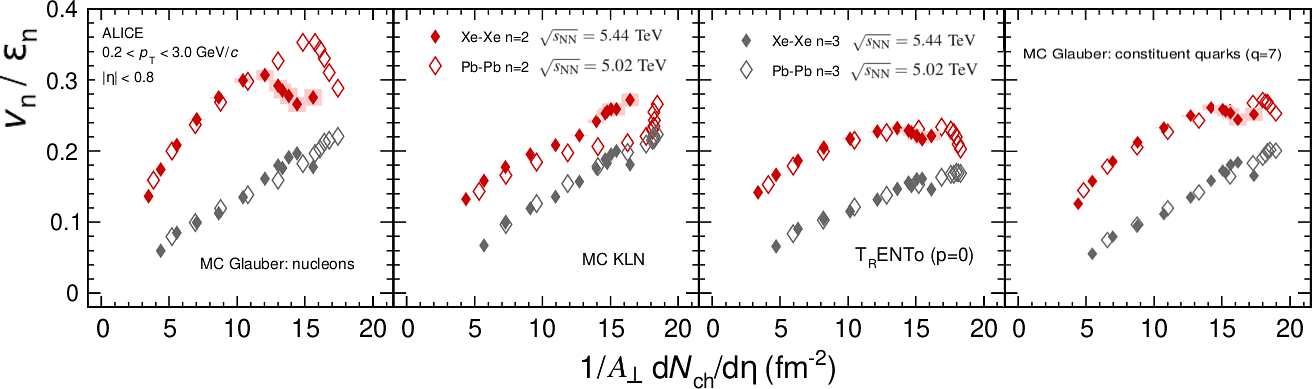
Figure 6: Comparisons of the ratio $v_{n}/\epsilon_{n}$ (for $n=2,3$) as a function of particle transverse density, $(1/A_{\perp}){\rm d}N_{\rm ch}/{\rm d}\eta$, in XeXe and PbPb collisions at the LHC, where $v_{n}$ and ${\rm d}N_{\rm ch}/{\rm d}\eta$ have been measured by the ALICE experiment, and the $\epsilon_{n}$ and $A_{\perp}$ parameters are derived using the ICs of various models described in the text. Figured adapted from Ref. [169].

Implications for the extraction of QGP transport properties, such as its viscosity constrained from the experimental ratio of triangular over elliptic flows ($v_{3}/v_{2}$), have also been studied e.g. in [119, 120] for UU collisions at RHIC energies. The work [119] shows that a model overestimation of the $\epsilon_{3}/\epsilon_{2}$ ratio will imply a larger amount of the viscous damping needed in the subsequent theoretical hydrodynamic evolution to match the experimental UU data. A critical comparison of ICs derived from IP-Glasma and MCG models for light systems produced in pAu and dAu collisions at RHIC can be found in Ref. [170].

5 EXPERIMENTAL DEVELOPMENTS

On the experimental front, the LHC data has provided a wealth of new results that have helped to improve the extraction of relevant quantities from the Glauber approach. We review here two experimental aspects of importance for the determination of the reaction centrality in pA and AA collisions. The centrality determination —a proxy for the (arguably) most important parameter of Glauber models: the collision impact parameter— is found to be subject to stronger biases at the LHC than at lower c.m. energies.

5.1 Collision Centrality Estimates

As mentioned earlier, neither the impact parameter nor any derived Glauber quantity can be directly measured experimentally. Instead, average quantities are obtained within Glauber approaches for classes of events whose inclusive particle multiplicities and/or energy distributions can be reproduced by the corresponding calculation over a given $b$ range. Since on average the impact parameter is monotonically related to the overall particle multiplicity, one typically measures multiplicity (or energy) distributions over a suitably large phase space. The mapping to calculated quantities then proceeds in intervals of centrality or centrality classes, which are obtained by binning the distribution in fractions of its total integral. Centrality is then typically defined as the percentile

$$c_{i}=\frac{c_{\rm ap}}{M_{\rm tot}}\,\int_{M_{\rm i}}^{\infty}\frac{\mathrm{d}N}{\mathrm{d}M}\,\mathrm{d}M\,,$$ (18)

of the per-event multiplicity distribution $\mathrm{d}N/\mathrm{d}M$ above $M_{\rm i}$ relative to

$$M_{\rm tot}=\int_{M_{\rm ap}}^{\infty}\frac{\mathrm{d}N}{\mathrm{d}M}\,\mathrm{d}M\,,$$ (19)

where $M_{\rm ap}$ ($<M_{i}$) is the multiplicity value for which the fraction of total cross section was determined at the $c_{\rm ap}$ point. The anchor point (AP) sets the absolute scale of the centrality. Clearly, one would like to achieve $M_{\rm ap}$ close to zero, resulting in $c_{\rm ap}$ close to 100%. However, because of trigger inefficiency and the increasing background contamination from ultraperipheral photonuclear collisions, experiments typically can only set the anchor point between 80 to 90% of the total hadronic cross section. An example is given in Fig. 7, which shows the sum of the amplitudes in the ALICE VZERO scintillators (at $2.8<\eta<5.1$ and $-1.7<\eta<-3.7$), called V0M centrality estimator, representing the uncorrected charged particle multiplicity distribution. The vertical lines indicate the typical centrality binning obtained from slicing the distribution in fractions of the total integral starting from 90% , where smaller fractions refer to more central collisions.

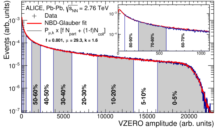
Figure 7: Distribution of the sum of amplitudes (V0M) in the ALICE VZERO detectors measured in PbPb collisions at $\!\sqrt{s_{{}_{\rm NN}}}=2.76$ TeV fitted with the NBD $+$ Glauber model. Centrality classes are indicated by vertical lines. The inset focuses on the most peripheral region. Figure from [171].

To determine the anchor point, two approaches are typically used. The first one involves simulation of hadronic and e.m. processes, including a detailed description of the detector response, and hence gives direct access to the fraction of hadronic events below $M_{\rm AP}$. The second one involves MCG modeling together with a simple description for particle production at detector level, to simulate the uncorrected multiplicity distribution. The calculated distribution will describe the data down to the most peripheral events up to some point where background contamination and trigger inefficiency start to matter. The point where data and simulation start to separate can be used to set the AP.

To model multiplicity in heavy-ion collisions, one exploits that the majority of the initial-state NN collisions can essentially be treated like MB pp collisions, with a small perturbation from rarer hard interactions. The charged particle multiplicity in minimum-bias pp collisions at high energy can be described by a negative binomial distribution (NBD) [86], given by

$$P_{\mu,k}(N_{\rm ch})=\frac{\Gamma(N_{\rm ch}+k)}{\Gamma(N_{\rm ch}+1)\Gamma(k)}\cdot\frac{(\mu/k)^{N_{\rm ch}}}{(\mu/k+1)^{N_{\rm ch}+k}}\,,$$ (20)

where $\mu$ is the mean and $k$ is related to the width of the multiplicity distribution. Hence, the multiplicity for heavy-ion events can be approximated as a superposition of many NBDs, quickly approaching the Gaussian limit. A typical approach is to assume that the number of particle emitting sources can be described by the two-component approach, $f\cdot N_{\rm part}+(1-f)\cdot N_{\rm coll}$ as in Eq. (4). A minimization procedure is then applied to the distribution of hadronic activity to determine the $\mu$, $k$, and $f$ parameters, with the values listed in Fig. 7 obtained with a $\chi^{2}/N_{\rm dof}$ close to unity. The AP can be determined with $\sim$1% uncertainty (absolute). The centrality resolution is at the level of as few % in peripheral collisions and better than 1% in most central collisions.

Due to the finite kinematic acceptance, trigger inefficiency, and detector resolution, as well as the possible biases of the event selection, the details of the centrality determination differ between experiments, and even among collision systems within a given experiment. A short introduction with references to the approaches at RHIC is given in [40], while for more details on similar approaches at the LHC, see [172, 171] for ALICE, [173] for CMS, and [174] for ATLAS. Alternative centrality estimators based on the transverse energy measured at forward rapidities (approx. $3<|\eta|<5$ for CMS and ATLAS), as well as far-forward neutral energy in Zero Degree Calorimeters (ZDCs) along the beam line [175, 171], have been also employed. The same methods can be applied to determine the centrality in pA or dAu collisions [176, 177, 178]. However, unlike for collisions of larger nuclei, the centrality determination is often subject to larger biases due to fluctuations in the categorization of events (see next section).

5.2 Collision Centrality Biases

As discussed in the previous section, medium effects on the production of perturbative QGP probes are in general quantified by the nuclear modification factor Eq. (16), defined as the ratio of the per-event yield measured in AA collisions over the same yield expected from an incoherent superposition of $N_{\rm coll}$ binary pp collisions. However, event centrality classification involves selection of event samples for which the properties of the underlying binary NN collisions may deviate from those of unbiased pp collisions [83]. In this case, $R_{\rm AA}$ (and $R_{\rm pA}$) can deviate from unity even in the absence of nuclear effects. There are two main sources of selection biases. First, the number of hard processes is suppressed for increasingly peripheral AA collisions because of a simple geometrical bias: the probability for collisions increases proportional to $b$ while the nuclear density decreases, leading to an increased probability for more-peripheral-than-average NN collisions. Second, the centrality selection, which relies mostly on measurements dominated by soft particle production —the relative weight of soft-to-hard contributions to the total energy distribution is given by the $f\approx 0.8$ parameter in Fig. 7— biases the average multiplicity of individual NN collisions, and hence can affect the normalization of yields of collisions dominated by hard processes. As shown in Fig. 3 (left), hard scatterings are more probable in central NN collisions with large partonic overlap thereby leading to many simultaneous MPIs with lots of UE activity, and since hard processes are dominated by the production of jets that fragment (or heavy resonances that decay) into a large number of final hadrons, a peripheral AA event with a hard scattering often has a hadronic activity much larger than that typical of its centrality class. Since the AA (and pA) centrality determination is based on ordering the measured multiplicity or summed energy in the event, peripheral nuclear events with a hard scattering can thereby be wrongly assigned to a more central class.

The geometrical effect can be included into optical Glauber calculations by extending Eq. (3) with a convolution of the nuclear thickness functions (depending on the overall $b$) with the NN overlap function ($T_{{}_{\rm NN}}$, depending on the $b_{{}_{\rm NN}}$ impact parameter) as

$$T_{{}_{\rm AB}}^{\prime}\left(\bf{b}\right)=\int{\rm d}^{2}{\rm s}\;{\rm d}^{2}b_{{}_{\rm NN}}\,T_{{}_{\rm A}}\left(\bf{s}\right)T_{{}_{\rm B}}\left(\bf{s}-\bf{b}+\bf{b_{{}_{\rm NN}}}\right)\,T_{{}_{\rm NN}}\left(\bf{b_{{}_{\rm NN}}}\right)\,,$$ (21)

which effectively leads to a reduction of $N_{\rm coll}$ in peripheral collisions compared to $T_{{}_{\rm NN}}=\delta(b_{{}_{\rm NN}})$ because of their increased probability for less-central-than-average NN collisions. Standard MCG calculations, which by construction include the geometrical bias, however, do not use information about individual NN collisions. Even though the NN collisions are still modeled as occurring incoherently, the number of hard processes for a given centrality selections is not taken proportional to $N_{\rm coll}$, but to

$$N_{\rm hard}=N_{\rm coll}\cdot N^{\rm hard}_{\rm NN}/\left<N^{\rm hard}_{\rm NN}\right>\,,$$ (22)

where $N^{\rm hard}_{\rm NN}$ is the average number of hard scatterings in a NN collision for a given centrality selection and $\left<N^{\rm hard}_{\rm NN}\right>$ is its unbiased average value. The mean number of hard scatterings per collision depends on $b_{{}_{\rm NN}}$, and can be written as $N_{\rm hard}(b_{{}_{\rm NN}})=\sigma_{\rm hard}\,T_{{}_{\rm NN}}(b_{{}_{\rm NN}})$, where $\sigma_{\rm hard}$ is the pQCD cross-section for $2\rightarrow 2$ parton scatterings. Since the yield of hard and soft processes are correlated via their common $b_{\rm NN}$, the NN collisions can be biased towards lower or higher than average impact parameters, when ordering the measured multiplicity or transverse energy necessary for the centrality determination. This leads to a selection bias on $N^{\rm hard}_{\rm NN}$ in addition to the inherent geometrical bias. Due to the strong dependence of $\sigma_{\rm hard}$ on $\sqrt{s}$, the selection bias is more relevant at LHC than at RHIC (and negligible at SPS) collision energies.

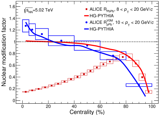
Figure 8: Nuclear modification factors for high-$p_{\rm T}$ charged particles (above 8 or 10 GeV) as a function of centrality in pPb (blue circles) and PbPb (red squares) collisions at $\!\sqrt{s_{{}_{\rm NN}}}=5.02$ TeV [177, 179] compared to calculations with hg-pythia [83] (blue and red curves, respectively).

The relevance of the selection bias induced by the correlation between soft and hard particles is demonstrated in Fig. 8 that shows the nuclear modification factors for charged particle production, integrated above a large enough $p_{\rm T}$ value (8 and 10 GeV), in pPb and PbPb collisions at $\!\sqrt{s_{{}_{\rm NN}}}=5.02$ TeV compared to calculations using hg-pythia [83]. The calculation, which uses the hijing model to determine the distribution of $N_{\rm hard}(b_{{}_{\rm NN}})$ in a nuclear collision and pythia 6.28 (Perugia 2011 tune) to generate the corresponding NN events, purposely does not include nuclear modification effects, unlike most of the models discussed in Sec. 4.2. As for the data, where the V0M estimator was used, the calculation determines the centrality using charged particles in the acceptance of the ALICE VZERO detectors. The calculation describes well the pPb and very peripheral PbPb data indicating that the strong apparent suppression from unity in this region results, in both cases, from the event selection. For more central PbPb collisions, where parton energy loss leads to the known, large suppression of particle production in PbPb compared to pp collisions, the $R_{\rm AA}$ is not affected by such biases.

The hard-soft event selection bias is particularly important when fluctuations of the centrality estimator caused by $b_{{}_{\rm NN}}$ are of similar size as the dynamic range of $N_{\rm coll}$, as is the case in pA collisions, and strongly enhanced by trivial autocorrelations if the phase space for the measurement and event categorization are close-by or overlap [176, 177, 178]. This can be already deduced by computing the ratio between the average multiplicity of the centrality estimator and the average multiplicity per average ancestor of the Glauber fit as demonstrated in Fig. 8 of [177]. In contrast, centrality measurements based on zero-degree energy should not introduce any selection bias, while the geometric bias could still play a role. In the so-called hybrid method, described in [177], the pPb centrality selection is based on ZDC neutral energy in the Pb-going directions (slow neutrons), and $N_{\rm coll}$ is determined from the measured charged particle multiplicity $M$ according to $N_{\rm coll}=\langle N_{\rm coll}\rangle\cdot M/\langle M\rangle$, where $\langle N_{\rm coll}\rangle$ and $\langle M\rangle$ are, respectively, the centrality-averaged number of collisions and multiplicity. In case soft and hard particle yields are affected in the same way, the selection bias would cancel out in the nuclear modification factor.

6 SUMMARY

An outstanding topic in the physics of the strong interaction is the understanding of the thermodynamic and transport properties of hot and dense quark-gluon matter accessible to experimental study via high-energy collisions of nuclei. To correctly identify and interpret signals of collective partonic behavior in AA collisions, it is necessary to have a realistic extrapolation of the baseline hadron production properties of pp and pA collisions where, in principle, no quark-gluon plasma (QGP) is expected to be formed. In this work, we have reviewed the main developments and the state-of-the-art of the Glauber approach to describe multiple scatterings in proton and nuclear collisions, after 10 years of operation with pp, pPb, and PbPb collisions at the CERN LHC, as well as with deformed light- and heavy-ions at BNL RHIC. The Glauber model allows for arguably the simplest, most economical, and yet successful, understanding of collisions of extended hadronic objects based on an impact-parameter ($b$) superposition of independent elementary scatterings, each of which produces particles and thereby defines the local and global density of the precursor QGP. Key derived quantities in Glauber models include the nuclear overlap function $T_{{}_{\rm AA}}(b)$, number of participant nucleons $N_{\rm part}(b)$, number of binary collisions $N_{\rm coll}(b)$, transverse area $A_{\perp}(b)$, eccentricities $\epsilon_{n}(b)$, average path-length $L(b)$, of the strongly-interaction medium produced at different collision centralities, which are fundamental for the extraction of the QGP properties from the data.

The new LHC measurements, performed at 50 times larger c.m. energies than at previous nuclear collisions, and the latest precision RHIC data for a variety of colliding systems, have required to revisit and improve various ingredients of the Monte Carlo Glauber (MCG) simulations. Our review has first provided a new fit of the world measurements of the inclusive inelastic nucleon-nucleon cross sections ($\sigma_{\rm NN}$), a key ingredient of MCG models. The inelastic hadronic pA and AA cross sections measured at the LHC are well reproduced by the corresponding MCG results derived using $\sigma_{\rm NN}$, a fact that confirms the overall validity of the Glauber model at the highest c.m. energies ever studied. Second, improved descriptions of the proton and nuclear density profiles, including subnucleonic degrees of freedom and neutron skin effects, and any associated sources of fluctuations and correlations, have been examined. Third, we have reviewed the main applications of the Glauber model for collider studies. The binary scaling prescription to quantitatively compare hard scattering cross sections in pp, pA, and AA collisions, has been validated by measurements of electroweak probes at the LHC whose yields are unaffected by final-state interactions in the QGP. The use of the Glauber formalism in MC event generators for heavy-ion physics, as well as to provide initial entropy-density profiles as input for relativistic hydrodynamics calculations, have also been discussed. The importance of a realistic description of the medium eccentricities to extract key transport properties, such as the QGP shear viscosity, from comparisons of elliptic and triangular flows measurements at RHIC and LHC to viscous hydrodynamics predictions has been highlighted. Last, the experimental procedures used and the inherent biases introduced by them, in the determination of the collision centrality from the data, which rely on the application of the MCG model, have been briefly discussed.

As an illustrative summary of our review, Fig. 9 shows the impact of different Glauber model ingredients and experimental biases, presented as a ratio as a function of centrality of the different elements over the default standard MCG calculation, for PbPb (left) and pPb (right) collisions at $\!\sqrt{s_{{}_{\rm NN}}}=5.5$ and 8.8 TeV, respectively. First, the red long-dashed curves indicate the magnitude of the experimental shift introduced in measured nuclear modification factors when not properly accounting for event selection (multiplicity- and process-dependent) biases introduced by the centrality determination. These biases are significant in the most peripheral centrality classes and need to be carefully modeled and/or corrected for, specially when aiming at precision measurements at large impact parameters. The other curves indicate the ratio of the values of $N_{\rm coll}$ obtained with modified ingredients with respect to standard MCG simulations. Inclusion of Glauber–Gribov fluctuations (via Eq. (10) with $\Omega=1$) , modified NN collision profiles (via Eq. (9) with $\omega=0.4$), or neutron skin effects, lead to few percent modifications of the $N_{\rm coll}$ values in different centrality ranges, in principle within the assigned Glauber model systematic uncertainties [18]. An analytical calculation of $N_{\rm coll}$ in the optical Glauber limit leads, however, to significant underestimations of the number of collisions for peripheral PbPb and pPb collisions.

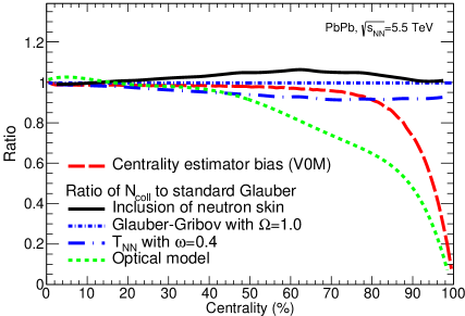
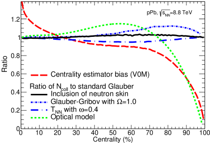
Figure 9: Ratio of $N_{\rm coll}$ as a function of centrality in PbPb (left) and pPb (right) collisions at the LHC obtained with the various model developments discussed in this review, and for the optical limit Eq. (3), normalized to the result obtained with the conventional MCG. In addition, the bias induced by the centrality determination is shown for a typical experimental estimator (ALICE V0M, long-dashed red curves).

The results of Fig. 9 emphasize large quantitative corrections needed in the Glauber model for the most peripheral AA and pA collisions. The availability of very large data samples of electroweak bosons at the LHC, with cross section measurements with few percent experimental uncertainties similar to or smaller than those of the Glauber model, opens up the possibility of using them to define an alternative experimental proxy for the nuclear overlap function. The ratio $N_{\rm V}/(\sigma_{\rm NN}^{\rm V}N_{\rm evt})$, where $\sigma_{\rm NN}^{\rm V}$ is the vector boson (V = $\sum W^{\pm}$, Z) production cross section in NN collisions (that can be estimated from pp measurements) and $N_{\rm V}/N_{\rm evt}$ the per-event AA yields, has been suggested [180] as a data-driven $T_{{}_{\rm AA}}(b)$ proxy that would eliminate the need for Glauber modeling, and reduce corrections for centrality and event-selection effects, while cancelling uncertainties in the determination of quantities such as $R_{\rm AA}$. Such a proposal would require a higher level of theoretical accuracy (next-to-next-to-leading order) in the nuclear parton distribution functions, and in their centrality dependence, in order to fully exploit the high-precision $\sigma_{\rm pp}^{\rm V}$ measurements.

All in all, the results summarized in this review show that, despite its simplicity (or, arguably, thanks to it), the Glauber model has stood for over 50 years as an indispensable and useful baseline approach to be able to quantitatively compare collisions of systems of varying size, from protons to uranium nuclei. Its continued exploitation to extract from the data key thermodynamics and transport properties of strongly interacting matter at the highest densities and temperature accessible in the laboratory, remains unchallenged for the years to come.

LICENSE

This work is licensed under CC-BY-4.0.

Appendix A Details on MCG simulations and parameters

This appendix provides a concise summary of technical details and parameters of MCG simulations. The MCG calculations for AA collisions are typically performed in two steps: (i) the nucleon positions in each colliding nucleus are determined for a given event, and (ii) the two nuclei are “collided” assuming that the nucleons travel in a straight-line along the beam axis (eikonal approximation). Conventional implementations can be found in the codes of Refs. [11, 12, 14, 15, 16, 17, 18, 19]. Among them, Refs. [16, 17] provide a simple approach to include subnucleonic degrees of freedom.

Setup of nuclei

The position of each nucleon in the nucleus is determined according to a probability density function, where one commonly requires a minimum internucleon separation ($d_{\rm min}=0.4$ fm) between the centers of the nucleons to mimic hard-core repulsion of nucleons inside the nucleus. The probability distribution for spherical nuclei is taken to be uniform in azimuthal and polar angles, and the radial probability function is taken from nuclear charge densities extracted in low-energy electron scattering experiments [20, 21]. The nuclear charge density is usually parametrized by a Fermi distribution with three parameters

$$\rho(r)=\rho_{0}\frac{1+w(r/R)^{2}}{1+\exp(\frac{r-R}{a})}\,,$$ (23)

where $R$ is the nuclear radius, $a$ is the skin depth, and $w$ is a parameter to describe deviations from a spherical shape. Values used for various nuclei are listed in Table 2. The overall normalization given by the nucleon density ($\rho_{0}$) plays no role in the MCG simulation.

Exceptions to Eq. (23) include the deuteron (²H), tritium (H3, ³H), helium-3 (He3, ³He), helium-4 (He4, ⁴He), carbon (C), oxygen (O), and sulfur (³²S) nuclei. For deuteron, three typical parametrizations are used:

1. The 3-parameter Fermi form, Eq. (23), with values $R=0.01$ fm, $a=0.5882$ fm, and $w=0$.

2. The Hulthén form:

   $$\rho(r^{\prime})=\rho_{0}\left(\frac{e^{-ar^{\prime}}-e^{-br^{\prime}}}{r^{\prime}}\right)^{2},$$ (24)

   where $a=0.228$ fm^-1 and $b=1.177$ fm^-1, and $r^{\prime}$ denotes the distance between the proton and neutron, i.e. $r=r^{\prime}/2$  [114, 115, 116].

3. The proton taken from the Hulthén form, Eq. (24), with the neutron placed opposite to it.

Name	$R$ [fm]	$a$ [fm]	$w$
28Si	3.340	0.5800	$-0.233$
32S	2.540	2.1910	0.16
40Ar	3.530	0.5420	0
40Ca	3.766	0.5860	$-0.161$
58Ni	4.309	0.5170	$-0.1308$
63Cu	4.200	0.5960	0
63CuHN	4.280	0.5000	0
129Xe	5.360	0.5900	0
129Xe	5.420	0.5700	0
186W	6.580	0.4800	0
197Au	6.380	0.5350	0
197AuHN	6.420	0.4400	0
207Pb	6.620	0.5460	0
207PbHN	6.650	0.4600	0
208Pb (prot)	$6.68$	$0.447$	0
208Pb (neut)	$6.69$	$0.560$	0

Table 2: Nuclear charge density parameters from [20, 21] for Eqs. (23) and (25). The suffix ’HN’ indicates rescaled values to account for finite nucleon profiles as derived in Ref. [182]. All configurations can be found in the TGlauNucleus::Lookup function of the TGlauberMC code [183].

For ³H and ³He, the configurations have been computed (and stored in a database) from Green’s function MC calculations using the AV18 + UIX model interactions, which correctly sample the position of the three nucleons, including correlations, as in Ref. [117]. These, and the results of wavefunction-based calculations for He-4, carbon, and oxygen derived in [118] are publicly available [183]. There are also rescaled values for the radius and skin depth of Cu (“CuHN”), Au (“AuHN”) and Pb (“PbHN”) to take into account the finite nucleon profile as derived in [182] and [119].

For sulfur, and a few other nuclei (Si, Ca, Ni,…), a 3-parameter Gaussian-like form is typically used

$$\rho(r)=\rho_{0}\frac{1+w(r/R)^{2}}{1+\exp(\frac{r^{2}-R^{2}}{a^{2}})}\,.$$ (25)

For deformed nuclei, one uses

$$\rho(x,y,z)=\rho_{0}\left\{{1+\exp\frac{\left(r-R(1+\beta_{2}Y_{20}+\beta_{4}Y_{40})\right)}{a}}\right\}^{-1}\,,$$ (26)

where $Y_{20}=\sqrt{\frac{5}{16\pi}}(3{\rm cos}^{2}(\theta)-1)$, $Y_{40}=\frac{3}{16\sqrt{\pi}}(35{\rm cos}^{4}(\theta)-30{\rm cos}^{2}(\theta)+3)$ with the deformation parameters $\beta_{2}$ and $\beta_{4}$ taken from [20, 21]. The values used for different nuclei (Al, Si, Cu, Xe, Au, and U) are listed in Table 3.

Name	$R$ [fm]	$a$ [fm]	$w$	$\beta_{2}$	$\beta_{4}$
27Al	3.340	0.5800	0	$-0.448$	-0.239
28Si2	3.340	0.5800	$-0.233$	$-0.478$	-0.250
63Cu2	4.200	0.5960	0	-0.162	$-0.006$
129Xe2	5.360	0.5900	0	0.161	$-0.003$
129Xe2	5.360	0.5900	0	0.18	-0
197Au2	6.380	0.5350	0	$-0.131$	$-0.031$
238U2	6.670	0.4400	0	-0.280	-0.093
238U	6.670	0.4400	0	-0.280	-0.093

Table 3: Nuclear charge density parameters for deformed nuclei from [20, 21]. The suffix ’2’ for Si2, Cu2, Au2, and U2 refers to the use of Eq. (26). All configurations can be found in the TGlauNucleus::Lookup function of the TGlauberMC code [183].

Collision of nuclei

After setting up the two nuclei, the impact parameter of the collision is chosen from ${\rm d}N/{\rm d}b\propto b$ up to some large maximum $b_{\rm max}$ with $b_{\rm max}>R_{A}+R_{B}\simeq 20\,$fm. The centers of the nuclei are shifted to $(-b/2,0,0)$ and $(b/2,0,0)$, respectively. The reaction plane, defined by the impact parameter and the beam direction, is given by the $x$- and $z$-axes, while the transverse plane is given by the $x$- and $y$-axes. The longitudinal coordinate is irrelevant in the calculation as the nucleons move along a straight trajectory along the beam axis.

The “ball diameter” defined as $D=\sqrt{\sigma_{\rm NN}/\pi}$ defines the interaction strength of two nucleons: Two nucleons from different nuclei are usually assumed to collide if their relative transverse distance is less than the ball diameter, i.e. $d<D$. Variants to this approach use nucleon overlap profles that differ from the hard-sphere (or “black-disc”) approach, as discussed in Sec. 3, see Eq. (9). If no nucleon–nucleon collision is registered for any pair of nucleons, then no nucleus–nucleus collision occurred. Counters for determination of the total (geometric) cross section are updated accordingly.

References

- [1] W. Busza, K. Rajagopal, and W. van der Schee, “Heavy Ion Collisions: The Big Picture, and the Big Questions,” Ann. Rev. Nucl. Part. Sci. 68 (2018) 339–376, arXiv:1802.04801 [hep-ph].
- [2] S. Borsanyi, Z. Fodor, C. Hoelbling, S. D. Katz, S. Krieg, and K. K. Szabo, “Full result for the QCD equation of state with 2+1 flavors,” Phys. Lett. B 730 (2014) 99–104, arXiv:1309.5258 [hep-lat].
- [3] HotQCD Collaboration, A. Bazavov et al., “Equation of state in (2+1)-flavor QCD,” Phys. Rev. D 90 (2014) 094503, arXiv:1407.6387 [hep-lat].
- [4] D. d’Enterria, “Quark-Gluon Matter,” J. Phys. G 34 (2007) S53–S82, arXiv:nucl-ex/0611012.
- [5] P. Martin and R. Glauber, “Relativistic theory of radiative orbital electron capture,” Phys. Rev. 109 (1958) 1307–1325.
- [6] R. J. Glauber and G. Matthiae, “High-energy scattering of protons by nuclei,” Nucl. Phys. B 21 (1970) 135–157.
- [7] W. Czyz and L. Maximon, “High-energy, small angle elastic scattering of strongly interacting composite particles,” Annals Phys. 52 (1969) 59–121.
- [8] A. Bialas, M. Bleszynski, and W. Czyz, “Multiplicity distributions in nucleus-nucleus collisions at high energies,” Nucl. Phys. B 111 (1976) 461–476.
- [9] A. Bialas, M. Bleszynski, and W. Czyz, “Relation between the Glauber model and classical probability calculus,” Acta Phys. Polon. B 8 (1977) 389–392.
- [10] X.-N. Wang and M. Gyulassy, “HIJING: A Monte Carlo model for multiple jet production in pp, pA and AA collisions,” Phys. Rev. D 44 (1991) 3501–3516.
- [11] W. Broniowski, M. Rybczynski, and P. Bozek, “GLISSANDO: Glauber initial-state simulation and more…,” Comput. Phys. Commun. 180 (2009) 69–83, arXiv:0710.5731 [nucl-th].
- [12] B. Alver, M. Baker, C. Loizides, and P. Steinberg, “The PHOBOS Glauber Monte Carlo,” arXiv:0805.4411 (2008) , arXiv:0805.4411 [nucl-ex].
- [13] M. Alvioli, H. J. Drescher, and M. Strikman, “A Monte Carlo generator of nucleon configurations in complex nuclei including nucleon-nucleon correlations,” Phys. Lett. B 680 (2009) 225–230, arXiv:0905.2670 [nucl-th].
- [14] M. Rybczynski, G. Stefanek, W. Broniowski, and P. Bozek, “GLISSANDO 2: GLauber Initial-State Simulation AND mOre…, ver. 2,” Comput. Phys. Commun. 185 (2014) 1759–1772, arXiv:1310.5475 [nucl-th].
- [15] C. Loizides, J. Nagle, and P. Steinberg, “Improved version of the PHOBOS Glauber Monte Carlo,” SoftwareX 1-2 (2015) 13–18, arXiv:1408.2549 [nucl-ex].
- [16] C. Loizides, “Glauber modeling of high-energy nuclear collisions at the subnucleon level,” Phys. Rev. C 94 (2016) 024914, arXiv:1603.07375 [nucl-ex].
- [17] J. T. Mitchell, D. V. Perepelitsa, M. J. Tannenbaum, and P. W. Stankus, “Tests of constituent-quark generation methods which maintain both the nucleon center of mass and the desired radial distribution in Monte Carlo Glauber models,” Phys. Rev. C 93 (2016) 054910, arXiv:1603.08836 [nucl-ex].
- [18] C. Loizides, J. Kamin, and D. d’Enterria, “Improved Monte Carlo Glauber predictions at present and future nuclear colliders,” Phys. Rev. C 97 (2018) 054910, arXiv:1710.07098 [nucl-ex]. [Erratum: Phys. Rev. C 99 (2019) 019901] http://tglaubermc.hepforge.org/.
- [19] P. Bożek, W. Broniowski, M. Rybczynski, and G. Stefanek, “GLISSANDO 3: GLauber Initial-State Simulation AND mOre…, ver. 3,” Comput. Phys. Commun. 245 (2019) 106850, arXiv:1901.04484 [nucl-th].
- [20] C. W. De Jager, H. De Vries, and C. De Vries, “Nuclear charge and magnetization density distribution parameters from elastic electron scattering,” Atom. Data Nucl. Data Tabl. 14 (1974) 479–508.
- [21] H. De Vries, C. W. De Jager, and C. De Vries, “Nuclear charge and magnetization density distribution parameters from elastic electron scattering,” Atom. Data Nucl. Data Tabl. 36 (1987) 495–536.
- [22] X.-N. Wang and M. Gyulassy, “Energy and centrality dependence of rapidity densities at RHIC,” Phys. Rev. Lett. 86 (2001) 3496–3499, arXiv:nucl-th/0008014.
- [23] J.-Y. Ollitrault, “Anisotropy as a signature of transverse collective flow,” Phys. Rev. D 46 (1992) 229–245.
- [24] P. Romatschke, “New developments in relativistic viscous hydrodynamics,” Int. J. Mod. Phys. E 19 (2010) 1–53, arXiv:0902.3663 [hep-ph].
- [25] D. A. Teaney, Viscous Hydrodynamics and the Quark Gluon Plasma, pp. 207–266. 2010. arXiv:0905.2433 [nucl-th].
- [26] M. Luzum and P. Romatschke, “Viscous hydrodynamic predictions for nuclear collisions at the LHC,” Phys. Rev. Lett. 103 (2009) 262302, arXiv:0901.4588 [nucl-th].
- [27] B. Schenke, S. Jeon, and C. Gale, “Elliptic and triangular flow in event-by-event (3+1)D viscous hydrodynamics,” Phys. Rev. Lett. 106 (2011) 042301, arXiv:1009.3244 [hep-ph].
- [28] U. Heinz and R. Snellings, “Collective flow and viscosity in relativistic heavy-ion collisions,” Ann. Rev. Nucl. Part. Sci. 63 (2013) 123–151, arXiv:1301.2826 [nucl-th].
- [29] R. D. Weller and P. Romatschke, “One fluid to rule them all: viscous hydrodynamic description of event-by-event central pp, pPb and PbPb collisions at TeV,” Phys. Lett. B 774 (2017) 351–356, arXiv:1701.07145 [nucl-th].
- [30] B. Alver and G. Roland, “Collision geometry fluctuations and triangular flow in heavy-ion collisions,” Phys. Rev. C 81 (2010) 054905, arXiv:1003.0194 [nucl-th]. [Erratum: Phys. Rev.C82,039903(2010)].
- [31] ALICE Collaboration, K. Aamodt et al., “Higher harmonic anisotropic flow measurements of charged particles in Pb-Pb collisions at =2.76 TeV,” Phys. Rev. Lett. 107 (2011) 032301, arXiv:1105.3865 [nucl-ex].
- [32] PHENIX Collaboration, A. Adare et al., “Measurements of higher-order flow harmonics in AuAu collisions at GeV,” Phys. Rev. Lett. 107 (2011) 252301, arXiv:1105.3928 [nucl-ex].
- [33] ATLAS Collaboration, G. Aad et al., “Measurement of the azimuthal anisotropy for charged particle production in TeV lead-lead collisions with the ATLAS detector,” Phys. Rev. C 86 (2012) 014907, arXiv:1203.3087 [hep-ex].
- [34] CMS Collaboration, S. Chatrchyan et al., “Multiplicity and transverse momentum Dependence of two- and four-particle correlations in pPb and PbPb collisions,” Phys. Lett. B 724 (2013) 213–240, arXiv:1305.0609 [nucl-ex].
- [35] A. Dainese, C. Loizides, and G. Paic, “Leading-particle suppression in high energy nucleus-nucleus collisions,” Eur. Phys. J. C 38 (2005) 461–474, arXiv:hep-ph/0406201 [hep-ph].
- [36] I. Lokhtin and A. Snigirev, “A model of jet quenching in ultrarelativistic heavy ion collisions and high- hadron spectra at RHIC,” Eur. Phys. J. C 45 (2006) 211–217, arXiv:hep-ph/0506189.
- [37] M. Djordjevic, D. Zigic, M. Djordjevic, and J. Auvinen, “How to test path-length dependence in energy loss mechanisms: analysis leading to a new observable,” Phys. Rev. C 99 (2019) 061902, arXiv:1805.04030 [nucl-th].
- [38] D. d’Enterria, “Jet quenching,” Landolt-Bornstein 23 (2010) 471, arXiv:0902.2011 [nucl-ex].
- [39] A. Baltz, “The Physics of ultraperipheral collisions at the LHC,” Phys. Rept. 458 (2008) 1–171, arXiv:0706.3356 [nucl-ex].
- [40] M. L. Miller, K. Reygers, S. J. Sanders, and P. Steinberg, “Glauber modeling in high energy nuclear collisions,” Ann. Rev. Nucl. Part. Sci. 57 (2007) 205–243, arXiv:nucl-ex/0701025 [nucl-ex].
- [41] PHOBOS Collaboration, B. Alver et al., “Phobos results on charged particle multiplicity and pseudorapidity distributions in Au+Au, Cu+Cu, d+Au, and p+p collisions at ultra-relativistic energies,” Phys. Rev. C 83 (2011) 024913, arXiv:1011.1940 [nucl-ex].
- [42] FCC Collaboration, A. Abada et al., “FCC-hh: The Hadron Collider: Future Circular Collider Conceptual Design Report Volume 3,” Eur. Phys. J. ST 228 (2019) 755–1107.
- [43] Particle Data Group Collaboration, M. Tanabashi et al., “Review of Particle Physics,” Phys. Rev. D 98 (2018) 030001.
- [44] UA5 Collaboration, G. J. Alner et al., “Antiproton-proton cross sections at 200 and 900 GeV c.m. energy,” Z. Phys. C 32 (1986) 153–161.
- [45] E710 Collaboration, N. A. Amos et al., “A luminosity independent measurement of the p total cross section at TeV,” Phys. Lett. B 243 (1990) 158–164.
- [46] E710 Collaboration, N. A. Amos et al., “Measurement of , the ratio of the real to imaginary part of the p forward elastic scattering amplitude, at TeV,” Phys. Rev. Lett. 68 (1992) 2433–2436.
- [47] CDF Collaboration, F. Abe et al., “Measurement of the total cross-section at GeV and 1800 GeV,” Phys. Rev. D 50 (1994) 5550–5561.
- [48] CDF Collaboration, F. Abe et al., “Measurement of small angle elastic scattering at GeV and 1800 GeV,” Phys. Rev. D 50 (1994) 5518–5534.
- [49] STAR Collaboration, J. Adam et al., “Results on total and elastic cross sections in proton-proton collisions at GeV,” Phys. Lett. B 808 (2020) 135663, arXiv:2003.12136 [hep-ex].
- [50] ALICE Collaboration, B. Abelev et al., “Measurement of inelastic, single- and double-diffraction cross sections in proton-proton collisions at the LHC with ALICE,” Eur. Phys. J. C 73 (2013) 2456, arXiv:1208.4968 [hep-ex].
- [51] ATLAS Collaboration, G. Aad et al., “Measurement of the inelastic proton-proton cross section at TeV with the ATLAS Detector,” Nature Commun. 2 (2011) 463, arXiv:1104.0326 [hep-ex].
- [52] ATLAS Collaboration, G. Aad et al., “Measurement of the total cross section from elastic scattering in pp collisions at TeV with the ATLAS detector,” Nucl. Phys. B 889 (2014) 486–548, arXiv:1408.5778 [hep-ex].
- [53] ATLAS Collaboration, M. Aaboud et al., “Measurement of the total cross section from elastic scattering in pp collisions at TeV with the ATLAS detector,” Phys. Lett. B 761 (2016) 158–178, arXiv:1607.06605 [hep-ex].
- [54] ATLAS Collaboration, M. Aaboud et al., “Measurement of the inelastic proton-proton cross section at TeV with the ATLAS detector at the LHC,” Phys. Rev. Lett. 117 (2016) 182002, arXiv:1606.02625 [hep-ex].
- [55] CMS Collaboration, S. Chatrchyan et al., “Measurement of the inelastic proton-proton cross section at TeV,” Phys. Lett. B 722 (2013) 5–27, arXiv:1210.6718 [hep-ex].
- [56] CMS Collaboration, A. M. Sirunyan et al., “Measurement of the inelastic proton-proton cross section at TeV,” JHEP 07 (2018) 161, arXiv:1802.02613 [hep-ex].
- [57] LHCb Collaboration, R. Aaij et al., “Measurement of the inelastic pp cross-section at a centre-of-mass energy of TeV,” JHEP 02 (2015) 129, arXiv:1412.2500 [hep-ex].
- [58] LHCb Collaboration, R. Aaij et al., “Measurement of the inelastic pp cross-section at a centre-of-mass energy of 13 TeV,” JHEP 06 (2018) 100, arXiv:1803.10974 [hep-ex].
- [59] TOTEM Collaboration, G. Antchev et al., “First measurement of the total proton-proton cross section at the LHC energy of TeV,” Europhys. Lett. 96 (2011) 21002, arXiv:1110.1395 [hep-ex].
- [60] TOTEM Collaboration, G. Antchev et al., “Luminosity-independent measurements of total, elastic and inelastic cross-sections at TeV,” Europhys. Lett. 101 (2013) 21004.
- [61] TOTEM Collaboration, G. Antchev et al., “Luminosity-independent measurement of the proton-proton total cross section at TeV,” Phys. Rev. Lett. 111 (2013) 012001.
- [62] TOTEM Collaboration, G. Antchev et al., “First measurement of elastic, inelastic and total cross-section at TeV by TOTEM and overview of cross-section data at LHC energies,” Eur. Phys. J. C 79 (2019) 103, arXiv:1712.06153 [hep-ex].
- [63] TOTEM Collaboration, F. Cafagna, “Latest results for proton-proton cross section measurements with the TOTEM experiment at LHC,” PoS ICRC2019 (2020) 207.
- [64] Pierre Auger Collaboration, P. Abreu et al., “Measurement of the proton-air cross-section at TeV with the Pierre Auger Observatory,” Phys. Rev. Lett. 109 (2012) 062002, arXiv:1208.1520 [hep-ex].
- [65] COMPETE Collaboration, J. R. Cudell et al., “Benchmarks for the forward observables at RHIC, the Tevatron Run II and the LHC,” Phys. Rev. Lett. 89 (2002) 201801, arXiv:hep-ph/0206172 [hep-ph].
- [66] D. d’Enterria and T. Pierog, “Global properties of proton-proton collisions at = 100 TeV,” JHEP 08 (2016) 170, arXiv:1604.08536 [hep-ph].
- [67] ALICE Collaboration, B. Abelev et al., “Measurement of the cross section for electromagnetic dissociation with neutron emission in PbPb collisions at TeV,” Phys. Rev. Lett. 109 (2012) 252302, arXiv:1203.2436 [nucl-ex].
- [68] CMS Collaboration, V. Khachatryan et al., “Measurement of the inelastic cross section in proton–lead collisions at 5.02 TeV,” Phys. Lett. B 759 (2016) 641–662, arXiv:1509.03893 [hep-ex].
- [69] ALICE Collaboration, B. B. Abelev et al., “Measurement of visible cross sections in proton-lead collisions at = 5.02 TeV in van der Meer scans with the ALICE detector,” JINST 9 (2014) P11003, arXiv:1405.1849 [nucl-ex].
- [70] T. Sjöstrand, S. Ask, J. R. Christiansen, R. Corke, N. Desai, P. Ilten, S. Mrenna, S. Prestel, C. O. Rasmussen, and P. Z. Skands, “An introduction to PYTHIA 8.2,” Comput. Phys. Commun. 191 (2015) 159–177, arXiv:1410.3012 [hep-ph].
- [71] M. Bahr et al., “Herwig++ Physics and Manual,” Eur. Phys. J. C 58 (2008) 639–707, arXiv:0803.0883 [hep-ph].
- [72] R. Field, “Min-Bias and the underlying event at the LHC,” Acta Phys. Polon. B 42 (2011) 2631–2656, arXiv:1110.5530 [hep-ph].
- [73] D. d’Enterria and A. Snigirev, “Double, triple, and -parton scatterings in high-energy proton and nuclear collisions,” Adv. Ser. Direct. High Energy Phys. 29 (2018) 159–187, arXiv:1708.07519 [hep-ph].
- [74] CMS Collaboration, V. Khachatryan et al., “Observation of long-range near-side angular correlations in proton-proton collisions at the LHC,” JHEP 09 (2010) 091, arXiv:1009.4122 [hep-ex].
- [75] ATLAS Collaboration, G. Aad et al., “Observation of long-range elliptic azimuthal anisotropies in 13 and 2.76 TeV pp collisions with the ATLAS Detector,” Phys. Rev. Lett. 116 (2016) 172301, arXiv:1509.04776 [hep-ex].
- [76] CMS Collaboration, V. Khachatryan et al., “Evidence for collectivity in pp collisions at the LHC,” Phys. Lett. B 765 (2017) 193–220, arXiv:1606.06198 [nucl-ex].
- [77] D. d’Enterria et al., “Estimates of hadron azimuthal anisotropy from multiparton interactions in proton-proton collisions at TeV,” Eur. Phys. J. C 66 (2010) 173–185, arXiv:0910.3029 [hep-ph].
- [78] R. Hofstadter, “Electron scattering and nuclear structure,” Rev. Mod. Phys. 28 (1956) 214–254.
- [79] R. Corke and T. Sjöstrand, “Multiparton Interactions with an -dependent proton size,” JHEP 05 (2011) 009, arXiv:1101.5953 [hep-ph].
- [80] P. Skands, S. Carrazza, and J. Rojo, “Tuning PYTHIA 8.1: the Monash 2013 tune,” Eur. Phys. J. C 74 (2014) 3024, arXiv:1404.5630 [hep-ph].
- [81] ALICE Collaboration, S. Acharya et al., “Charged-particle production as a function of multiplicity and transverse spherocity in pp collisions at and 13 TeV,” Eur. Phys. J. C 79 (2019) 857, arXiv:1905.07208 [nucl-ex].
- [82] T. Sjöstrand, “The development of MPI modeling in PYTHIA,” Adv. Ser. Direct. High Energy Phys. 29 (2018) 191–225, arXiv:1706.02166 [hep-ph].
- [83] C. Loizides and A. Morsch, “Absence of jet quenching in peripheral nucleus-–nucleus collisions,” Phys. Lett. B 773 (2017) 408–411, arXiv:1705.08856 [nucl-ex].
- [84] M. Alvioli, H. Holopainen, K. J. Eskola, and M. Strikman, “Initial state anisotropies and their uncertainties in ultrarelativistic heavy-ion collisions from the Monte Carlo Glauber model,” Phys. Rev. C 85 (2012) 034902, arXiv:1112.5306 [hep-ph].
- [85] M. Rybczyński and Z. Wlodarczyk, “The nucleon-nucleon collision profile and cross section fluctuations,” J. Phys. G 41 (2013) 015106, arXiv:1307.0636 [nucl-th].
- [86] J. F. Grosse-Oetringhaus and K. Reygers, “Charged-Particle Multiplicity in Proton-Proton Collisions,” J. Phys. G 37 (2010) 083001, arXiv:0912.0023 [hep-ex].
- [87] K. Welsh, J. Singer, and U. W. Heinz, “Initial state fluctuations in collisions between light and heavy ions,” Phys. Rev. C 94 (2016) 024919, arXiv:1605.09418 [nucl-th].
- [88] J. S. Moreland, J. E. Bernhard, and S. A. Bass, “Bayesian calibration of a hybrid nuclear collision model using pPb and PbPb data at energies available at the CERN Large Hadron Collider,” Phys. Rev. C 101 (2020) 024911, arXiv:1808.02106 [nucl-th].
- [89] D. Teaney and L. Yan, “Triangularity and dipole asymmetry in heavy ion collisions,” Phys. Rev. C 83 (2011) 064904, arXiv:1010.1876 [nucl-th].
- [90] PHOBOS Collaboration, B. Alver et al., “System size, energy, pseudorapidity, and centrality dependence of elliptic flow,” Phys. Rev. Lett. 98 (2007) 242302, arXiv:nucl-ex/0610037 [nucl-ex].
- [91] J.-P. Blaizot, W. Broniowski, and J.-Y. Ollitrault, “Correlations in the Monte Carlo Glauber model,” Phys. Rev. C 90 (2014) 034906, arXiv:1405.3274 [nucl-th].
- [92] H. Heiselberg, G. Baym, B. Blaettel, L. Frankfurt, and M. Strikman, “Color transparency, color opacity, and fluctuations in nuclear collisions,” Phys. Rev. Lett. 67 (1991) 2946–2949.
- [93] M. Alvioli and M. Strikman, “Color fluctuation effects in proton-nucleus collisions,” Phys. Lett. B 722 (2013) 347–354, arXiv:1301.0728 [hep-ph].
- [94] M. Alvioli, L. Frankfurt, D. Perepelitsa, and M. Strikman, “Global analysis of color fluctuation effects in proton– and deuteron–nucleus collisions at RHIC and the LHC,” Phys. Rev. D 98 (2018) 071502, arXiv:1709.04993 [hep-ph].
- [95] V. Gribov, “Glauber corrections and the interaction between high-energy hadrons and nuclei,” Sov. Phys. JETP 29 (1969) 483–487.
- [96] C. Bierlich, G. Gustafson, and L. Lönnblad, “Diffractive and non-diffractive wounded nucleons and final states in pA collisions,” JHEP 10 (2016) 139, arXiv:1607.04434 [hep-ph].
- [97] PHENIX Collaboration, A. Adare et al., “Centrality-dependent modification of jet-production rates in deuteron-gold collisions at =200 GeV,” Phys. Rev. Lett. 116 (2016) 122301, arXiv:1509.04657 [nucl-ex].
- [98] ATLAS Collaboration, G. Aad et al., “Measurement of the centrality dependence of the charged-particle pseudorapidity distribution in pPb collisions at TeV with the ATLAS detector,” Eur. Phys. J. C 76 (2016) 199, arXiv:1508.00848 [hep-ex].
- [99] D. McGlinchey, J. Nagle, and D. Perepelitsa, “Consequences of high- proton size fluctuations in small collision systems at 200 GeV,” Phys. Rev. C 94 (2016) 024915, arXiv:1603.06607 [nucl-th].
- [100] C. Ciofi degli Atti, B. Kopeliovich, C. Mezzetti, I. Potashnikova, and I. Schmidt, “Number of collisions in the Glauber Model and beyond,” Phys. Rev. C 84 (2011) 025205, arXiv:1105.1080 [nucl-th].
- [101] C. Flensburg, G. Gustafson, and L. Lönnblad, “Inclusive and exclusive observables from dipoles in high energy collisions,” JHEP 08 (2011) 103, arXiv:1103.4321 [hep-ph].
- [102] G. Salam, “A resummation of large subleading corrections at small ,” JHEP 07 (1998) 019, arXiv:hep-ph/9806482.
- [103] R. C. Barrett and D. F. Jackson, Nuclear sizes and structure. Oxford University Press, 1977.
- [104] B. Klos et al., “Neutron density distributions from antiprotonic 208Pb and 209Bi atoms,” Phys. Rev. C 76 (2007) 014311, arXiv:nucl-ex/0702016 [NUCL-EX].
- [105] C. M. Tarbert et al., “Neutron skin of 208Pb from coherent pion photoproduction,” Phys. Rev. Lett. 112 (2014) 242502, arXiv:1311.0168 [nucl-ex].
- [106] G. Fricke, C. Bernhardt, K. Heilig, L. A. Schaller, L. Schellenberg, E. B. Shera, and C. W. de Jager, “Nuclear Ground State Charge Radii from Electromagnetic Interactions,” Atom. Data Nucl. Data Tabl. 60 (1995) 177.
- [107] C. J. Horowitz, S. J. Pollock, P. A. Souder, and R. Michaels, “Parity violating measurements of neutron densities,” Phys. Rev. C 63 (2001) 025501, arXiv:nucl-th/9912038 [nucl-th].
- [108] H. Paukkunen, “Neutron skin and centrality classification in high-energy heavy-ion collisions at the LHC,” Phys. Lett. B 745 (2015) 73–78, arXiv:1503.02448 [hep-ph].
- [109] S. De, “The effect of neutron skin on inclusive prompt photon production in PbPb collisions at Large Hadron Collider energies,” J. Phys. G 44 (2017) 045104, arXiv:1609.09608 [nucl-th].
- [110] I. Helenius, H. Paukkunen, and K. J. Eskola, “Neutron-skin effect in direct-photon and charged hadron-production in PbPb collisions at the LHC,” Eur. Phys. J. C 77 (2017) 148, arXiv:1606.06910 [hep-ph].
- [111] M. Alvioli and M. Strikman, “Spin-isospin correlated configurations in complex nuclei and neutron skin effect in W± production in high-energy proton-lead collisions,” Phys. Rev. C 100 (2019) 024912, arXiv:1811.10078 [hep-ph].
- [112] PHENIX Collaboration, J. M. Durham, “PHENIX results on system size dependence of J/ nuclear modification in 3He+A collisions at =200 GeV,” PoS HardProbes2018 (2018) 165, arXiv:1812.08889 [nucl-ex].
- [113] STAR Collaboration, L. Adamczyk et al., “Azimuthal anisotropy in UU and AuAu collisions at RHIC,” Phys. Rev. Lett. 115 (2015) 222301, arXiv:1505.07812 [nucl-ex].
- [114] L. Hulthén and M. Sugawara, The two-nucleon problem, pp. 1–143. Springer Berlin Heidelberg, Berlin, Heidelberg, 1957.
- [115] PHENIX Collaboration, S. S. Adler et al., “Absence of suppression in particle production at large transverse momentum in GeV dAu collisions,” Phys. Rev. Lett. 91 (2003) 072303, arXiv:nucl-ex/0306021 [nucl-ex].
- [116] PHENIX Collaboration, S. S. Adler et al., “Nuclear effects on hadron production in dAu and pp collisions at GeV,” Phys. Rev. C 74 (2006) 024904, arXiv:nucl-ex/0603010 [nucl-ex].
- [117] J. L. Nagle et al., “Exploiting intrinsic triangular geometry in relativistic 3HeAu collisions to disentangle medium properties,” Phys. Rev. Lett. 113 (2014) 112301, arXiv:1312.4565 [nucl-th].
- [118] S. Lim et al., “Exploring new small system geometries in heavy ion collisions,” Phys. Rev. C 99 (2019) 044904, arXiv:1812.08096 [nucl-th].
- [119] Q. Y. Shou, Y. G. Ma, P. Sorensen, A. H. Tang, F. Videbæk, and H. Wang, “Parameterization of deformed nuclei for Glauber modeling in relativistic heavy-ion collisions,” Phys. Lett. B 749 (2015) 215–220, arXiv:1409.8375 [nucl-th].
- [120] J. Noronha-Hostler, N. Paladino, S. Rao, M. D. Sievert, and D. E. Wertepny, “Ultracentral collisions of small and deformed systems at RHIC: UU, dAu, 9BeAu, 9Be9Be 3He3He, and 3HeAu collisions,” arXiv:1905.13323 [hep-ph].
- [121] G. Giacalone, “Observing the deformation of nuclei with relativistic nuclear collisions,” Phys. Rev. Lett. 124 (2020) 202301, arXiv:1910.04673 [nucl-th].
- [122] S. Huang, Z. Chen, J. Jia, and W. Li, “Disentangling contributions to small-system collectivity via scans of light nucleus-nucleus collisions,” Phys. Rev. C 101 (2020) 021901, arXiv:1904.10415 [nucl-ex].
- [123] M. D. Sievert and J. Noronha-Hostler, “CERN Large Hadron Collider system size scan predictions for PbPb, XeXe, ArAr, and OO with relativistic hydrodynamics,” Phys. Rev. C 100 (2019) 024904, arXiv:1901.01319 [nucl-th].
- [124] R. Vogt, “Relation of hard and total cross-sections to centrality,” Acta Phys. Hung. A 9 (1999) 339–348, arXiv:nucl-th/9903051.
- [125] D. d’Enterria, “Hard scattering cross-sections at LHC in the Glauber approach: From pp to pA and AA collisions,” arXiv:nucl-ex/0302016 [nucl-ex].
- [126] PHENIX Collaboration, S. Adler et al., “Centrality dependence of direct photon production in =200 GeV AuAu collisions,” Phys. Rev. Lett. 94 (2005) 232301, arXiv:nucl-ex/0503003.
- [127] CMS Collaboration, S. Chatrchyan et al., “Measurement of isolated photon production in pp and PbPb collisions at TeV,” Phys. Lett. B 710 (2012) 256–277, arXiv:1201.3093 [nucl-ex].
- [128] ATLAS Collaboration, G. Aad et al., “Centrality, rapidity and transverse momentum dependence of isolated prompt photon production in lead-lead collisions at TeV measured with the ATLAS detector,” Phys. Rev. C 93 (2016) 034914, arXiv:1506.08552 [hep-ex].
- [129] CMS Collaboration, A. M. Sirunyan et al., “The production of isolated photons in PbPb and pp collisions at TeV,” JHEP 07 (2020) 116, arXiv:2003.12797 [hep-ex].
- [130] ATLAS Collaboration, G. Aad et al., “Measurement of boson production in PbPb collisions at TeV with the ATLAS detector,” Phys. Rev. Lett. 110 (2013) 022301, arXiv:1210.6486 [hep-ex].
- [131] ATLAS Collaboration, G. Aad et al., “Measurement of the production and lepton charge asymmetry of bosons in PbPb collisions at TeV with the ATLAS detector,” Eur. Phys. J. C 75 (2015) 23, arXiv:1408.4674 [hep-ex].
- [132] ATLAS Collaboration, G. Aad et al., “ boson production in pPb collisions at TeV measured with the ATLAS detector,” Phys. Rev. C 92 (2015) 044915, arXiv:1507.06232 [hep-ex].
- [133] CMS Collaboration, V. Khachatryan et al., “Study of Z boson production in pPb collisions at TeV,” Phys. Lett. B 759 (2016) 36–57, arXiv:1512.06461 [hep-ex].
- [134] ALICE Collaboration, S. Acharya et al., “Measurement of Z0-boson production at large rapidities in Pb-Pb collisions at TeV,” Phys. Lett. B 780 (2018) 372–383, arXiv:1711.10753 [nucl-ex].
- [135] ATLAS Collaboration, G. Aad et al., “ boson production in PbPb collisions at =5.02 TeV measured by the ATLAS experiment,” Phys. Lett. B 802 (2020) 135262, arXiv:1910.13396 [nucl-ex].
- [136] ATLAS Collaboration, G. Aad et al., “Measurement of boson production in PbPb collisions at TeV with the ATLAS detector,” Eur. Phys. J. C 79 (2019) 935, arXiv:1907.10414 [nucl-ex].
- [137] CMS Collaboration, A. M. Sirunyan et al., “Observation of nuclear modifications in W± boson production in pPb collisions at TeV,” Phys. Lett. B 800 (2020) 135048, arXiv:1905.01486 [hep-ex].
- [138] K. J. Eskola, P. Paakkinen, H. Paukkunen, and C. A. Salgado, “EPPS16: Nuclear parton distributions with LHC data,” Eur. Phys. J. C 77 (2017) 163, arXiv:1612.05741 [hep-ph].
- [139] A. Kusina et al., “Vector boson production in pPb and PbPb collisions at the LHC and its impact on nCTEQ15 PDFs,” Eur. Phys. J. C 77 (2017) 488, arXiv:1610.02925 [nucl-th].
- [140] R. Abdul Khalek, J. J. Ethier, J. Rojo, and G. van Weelden, “nNNPDF2.0: quark flavor separation in nuclei from LHC data,” JHEP 09 (2020) 183, arXiv:2006.14629 [hep-ph].
- [141] H. Khanpour and S. Atashbar Tehrani, “Global analysis of nuclear parton distribution functions and their uncertainties at next-to-next-to-leading order,” Phys. Rev. D 93 (2016) 014026, arXiv:1601.00939 [hep-ph].
- [142] K. J. Eskola, I. Helenius, M. Kuha, and H. Paukkunen, “Shadowing in inelastic nucleon-nucleon cross section?,” Phys. Rev. Lett. 125 (2020) 212301, arXiv:2003.11856 [hep-ph].
- [143] W.-T. Deng, X.-N. Wang, and R. Xu, “Hadron production in pp, pPb, and PbPb collisions with the HIJING 2.0 model at energies available at the CERN Large Hadron Collider,” Phys. Rev. C 83 (2011) 014915, arXiv:1008.1841 [hep-ph].
- [144] T. Pierog, I. Karpenko, J. Katzy, E. Yatsenko, and K. Werner, “EPOS LHC: Test of collective hadronization with data measured at the CERN Large Hadron Collider,” Phys. Rev. C 92 (2015) 034906, arXiv:1306.0121 [hep-ph].
- [145] Z.-W. Lin, C. M. Ko, B.-A. Li, B. Zhang, and S. Pal, “A Multi-phase transport model for relativistic heavy ion collisions,” Phys. Rev. C 72 (2005) 064901, arXiv:nucl-th/0411110.
- [146] S. Ostapchenko, “Monte Carlo treatment of hadronic interactions in enhanced Pomeron scheme: I. QGSJET-II model,” Phys. Rev. D 83 (2011) 014018, arXiv:1010.1869 [hep-ph].
- [147] S. Roesler, R. Engel, and J. Ranft, “The Monte Carlo event generator DPMJET-III,” in Intl. Conf. on Adv. Monte Carlo for Rad. Phys., Part. Transp. Simul. and Appl. (MC 2000), pp. 1033–1038. 12, 2000. arXiv:hep-ph/0012252.
- [148] T. Sjöstrand, S. Mrenna, and P. Z. Skands, “A Brief Introduction to PYTHIA 8.1,” Comput. Phys. Commun. 178 (2008) 852–867, arXiv:0710.3820 [hep-ph].
- [149] C. Bierlich, G. Gustafson, L. Lönnblad, and H. Shah, “The Angantyr model for heavy-ion collisions in PYTHIA8,” JHEP 10 (2018) 134, arXiv:1806.10820 [hep-ph].
- [150] D. d’Enterria, R. Engel, T. Pierog, S. Ostapchenko, and K. Werner, “Constraints from the first LHC data on hadronic event generators for ultra-high energy cosmic-ray physics,” Astropart. Phys. 35 (2011) 98–113, arXiv:1101.5596 [astro-ph.HE].
- [151] B. Andersson, The Lund model, vol. 7. Cambridge University Press, 7, 2005.
- [152] B. Andersson, G. Gustafson, and B. Nilsson-Almqvist, “A model for low hadronic reactions, with generalizations to hadron–nucleus and nucleus–nucleus collisions,” Nucl. Phys. B 281 (1987) 289–309.
- [153] S. R. Klein, J. Nystrand, J. Seger, Y. Gorbunov, and J. Butterworth, “STARlight: A Monte Carlo simulation program for ultra-peripheral collisions of relativistic ions,” Comput. Phys. Commun. 212 (2017) 258–268, arXiv:1607.03838 [hep-ph].
- [154] L. Harland-Lang, V. Khoze, and M. Ryskin, “Exclusive LHC physics with heavy ions: SuperChic 3,” Eur. Phys. J. C 79 (2019) 39, arXiv:1810.06567 [hep-ph].
- [155] U. W. Heinz, Early collective expansion: Relativistic hydrodynamics and the transport properties of QCD matter, vol. 23, p. 240. 2010. arXiv:0901.4355 [nucl-th].
- [156] T. Hirano, P. Huovinen, K. Murase, and Y. Nara, “Integrated dynamical approach to relativistic heavy ion collisions,” Prog. Part. Nucl. Phys. 70 (2013) 108–158, arXiv:1204.5814 [nucl-th].
- [157] C. Gale, S. Jeon, and B. Schenke, “Hydrodynamic modeling of heavy-ion collisions,” Int. J. Mod. Phys. A 28 (2013) 1340011, arXiv:1301.5893 [nucl-th].
- [158] H. Petersen, J. Steinheimer, G. Burau, M. Bleicher, and H. Stocker, “A fully integrated transport approach to heavy ion reactions with an intermediate hydrodynamic sStage,” Phys. Rev. C 78 (2008) 044901, arXiv:0806.1695 [nucl-th].
- [159] M. Strickland, “Thermalization and isotropization in heavy-ion collisions,” Pramana 84 (2015) 671–684, arXiv:1312.2285 [hep-ph].
- [160] D. Kharzeev, E. Levin, and M. Nardi, “The Onset of classical QCD dynamics in relativistic heavy ion collisions,” Phys. Rev. C 71 (2005) 054903, arXiv:hep-ph/0111315.
- [161] H.-J. Drescher and Y. Nara, “Effects of fluctuations on the initial eccentricity from the Color Glass Condensate in heavy ion collisions,” Phys. Rev. C 75 (2007) 034905, arXiv:nucl-th/0611017.
- [162] B. Schenke, P. Tribedy, and R. Venugopalan, “Event-by-event gluon multiplicity, energy density, and eccentricities in ultrarelativistic heavy-ion collisions,” Phys. Rev. C 86 (2012) 034908, arXiv:1206.6805 [hep-ph].
- [163] B. Schenke, P. Tribedy, and R. Venugopalan, “Fluctuating Glasma initial conditions and flow in heavy ion collisions,” Phys. Rev. Lett. 108 (2012) 252301, arXiv:1202.6646 [nucl-th].
- [164] F. Gelis, E. Iancu, J. Jalilian-Marian, and R. Venugopalan, “The Color Glass Condensate,” Ann. Rev. Nucl. Part. Sci. 60 (2010) 463–489, arXiv:1002.0333 [hep-ph].
- [165] K. Eskola, K. Kajantie, P. Ruuskanen, and K. Tuominen, “Scaling of transverse energies and multiplicities with atomic number and energy in ultrarelativistic nuclear collisions,” Nucl. Phys. B 570 (2000) 379–389, arXiv:hep-ph/9909456.
- [166] H. Niemi, K. Eskola, and R. Paatelainen, “Event-by-event fluctuations in a perturbative QCD + saturation + hydrodynamics model: Determining QCD matter shear viscosity in ultrarelativistic heavy-ion collisions,” Phys. Rev. C 93 (2016) 024907, arXiv:1505.02677 [hep-ph].
- [167] J. S. Moreland, J. E. Bernhard, and S. A. Bass, “Alternative ansatz to wounded nucleon and binary collision scaling in high-energy nuclear collisions,” Phys. Rev. C 92 (2015) 011901, arXiv:1412.4708 [nucl-th].
- [168] H. Kowalski and D. Teaney, “An Impact parameter dipole saturation model,” Phys. Rev. D 68 (2003) 114005, arXiv:hep-ph/0304189.
- [169] ALICE Collaboration, S. Acharya et al., “Anisotropic flow in XeXe collisions at TeV,” Phys. Lett. B 784 (2018) 82–95, arXiv:1805.01832 [nucl-ex].
- [170] J. Nagle and W. Zajc, “Assessing saturation physics explanations of collectivity in small collision systems with the IP-Jazma model,” Phys. Rev. C 99 (2019) 054908, arXiv:1808.01276 [nucl-th].
- [171] ALICE Collaboration, B. Abelev et al., “Centrality determination of PbPb collisions at TeV with ALICE,” Phys. Rev. C 88 (2013) 044909, arXiv:1301.4361 [nucl-ex].
- [172] ALICE Collaboration, S. Acharya, “Centrality determination in heavy ion collisions,” ALICE-PUBLIC-2018-011 (8, 2018) . https://cds.cern.ch/record/2636623.
- [173] CMS Collaboration, S. Chatrchyan et al., “Dependence on pseudorapidity and centrality of charged hadron production in PbPb collisions at a nucleon-nucleon centre-of-mass energy of 2.76 TeV,” JHEP 08 (2011) 141, arXiv:1107.4800 [nucl-ex].
- [174] ATLAS Collaboration, G. Aad et al., “Measurement of the centrality dependence of the charged particle pseudorapidity distribution in lead-lead collisions at TeV with the ATLAS detector,” Phys. Lett. B 710 (2012) 363–382, arXiv:1108.6027 [hep-ex].
- [175] J. S. Wood, The development of the CMS Zero Degree Calorimeters to derive the centrality of AA collisions. PhD thesis, Kansas U., 2012.
- [176] PHENIX Collaboration, A. Adare et al., “Centrality categorization for in high-energy collisions,” Phys. Rev. C 90 (2014) 034902, arXiv:1310.4793 [nucl-ex].
- [177] ALICE Collaboration, J. Adam et al., “Centrality dependence of particle production in pPb collisions at = 5.02 TeV,” Phys. Rev. C 91 (2015) 064905, arXiv:1412.6828 [nucl-ex].
- [178] D. V. Perepelitsa and P. A. Steinberg, “Calculation of centrality bias factors in pA collisions based on a positive correlation of hard process yields with underlying event activity,” arXiv:1412.0976 [nucl-ex].
- [179] ALICE Collaboration, S. Acharya et al., “Analysis of the apparent nuclear modification in peripheral PbPb collisions at 5.02 TeV,” Phys. Lett. B 793 (2019) 420–432, arXiv:1805.05212 [nucl-ex].
- [180] CMS Collaboration, “New constraints of initial states in PbPb collisions with Z boson yields and azimuthal anisotropy at TeV,” http://inspirehep.net/literature/1799323 (6, 2020) .
- [181] K. Tsukada et al., “First elastic electron scattering from 132Xe at the SCRIT facility,” Phys. Rev. Lett. 118 (2017) 262501, arXiv:1703.04278 [nucl-ex].
- [182] T. Hirano and Y. Nara, “Eccentricity fluctuation effects on elliptic flow in relativistic heavy ion collisions,” Phys. Rev. C 79 (2009) 064904, arXiv:0904.4080 [nucl-th].
- [183] “TGlauberMC on HepForge.” http://tglaubermc.hepforge.org/. v3.2.
- [184] W. Fischer and others, “Isotope shifts in the atomic spectrum of xenon and nuclear deformation effects,” Z. Physik 270 (1974) 113.
- [185] ALICE Collaboration, S. Acharya and others, “Centrality determination using the Glauber model in XeXe collisions at TeV,”. https://cds.cern.ch/record/2315401.
- [186] U. W. Heinz and A. Kuhlman, “Anisotropic flow and jet quenching in ultrarelativistic UU collisions,” Phys. Rev. Lett. 94 (2005) 132301, arXiv:nucl-th/0411054 [nucl-th].