A high-genus asymptotic expansion of
Weil–Petersson volume polynomials

Abstract

The object under consideration in this article is the total volume $V_{g,n}(x_{1},\ldots,x_{n})$ of the moduli space of hyperbolic surfaces of genus $g$ with $n$ boundary components of lengths $x_{1},\ldots,x_{n}$, for the Weil–Petersson volume form. We prove the existence of an asymptotic expansion of the quantity $V_{g,n}(x_{1},\ldots,x_{n})$ in terms of negative powers of the genus $g$, true for fixed $n$ and any $x_{1},\ldots,x_{n}\geq 0$. The first term of this expansion appears in work of Mirzakhani and Petri (2019), and we compute the second term explicitly. The main tool used in the proof is Mirzakhani’s topological recursion formula, for which we provide a comprehensive introduction.

1 Introduction and statement of the results

1.1 First definitions and notations

Let $g$, $n$ be two integers such that $2g-2+n>0$. For any given length vector $\mathbf{x}=(x_{1},\ldots,x_{n})\in\mathbb{R}_{\geq 0}^{n}$, we define the moduli space $\mathcal{M}_{g,n}(\mathbf{x})$ to be the set of isometry classes of surfaces $X$ satisfying the following:

• $X$ is a connected oriented hyperbolic surface of genus $g$ with $n$ labelled boundary components $b_{1},\ldots,b_{n}$,

• for all $i\in\{1,\ldots,n\}$, the boundary components $b_{i}$ is a closed geodesic of length $x_{i}$ if $x_{i}>0$, or a cusp if $x_{i}=0$.

This space is an orbifold of dimension $6g-6+2n$. It is equipped with a natural symplectic form, the Weil–Petersson form $\omega^{\mathrm{WP}}_{g,n,\mathbf{x}}$ [Wei58, Gol84], which canonically induces a volume form

$$\mathrm{Vol}^{\mathrm{\scriptsize{WP}}}_{g,n,\mathbf{x}}:=\frac{1}{(3g-3+n)!}\underbrace{\omega^{\mathrm{WP}}_{g,n,\mathbf{x}}\wedge\ldots\wedge\omega^{\mathrm{WP}}_{g,n,\mathbf{x}}}_{3g-3+n\text{ times}}.$$

The object under consideration in this article is the total volume of the moduli space,

$$V_{g,n}(\mathbf{x}):=\mathrm{Vol}^{\mathrm{\scriptsize{WP}}}_{g,n,\mathbf{x}}(\mathcal{M}_{g,n}(\mathbf{x}))<+\infty.$$

By work of Mirzakhani, [Mir07a], the volume $V_{g,n}(\mathbf{x})$ is a symmetric polynomial function in $x_{1}^{2},\ldots,x_{n}^{2}$ of degree $3g-3+n$, and can therefore be written as

$$V_{g,n}(\mathbf{x})=\sum_{\begin{subarray}{c}\alpha_{1}+\ldots+\alpha_{n}\\ \leq 3g-3+n\end{subarray}}c_{g,n}(\alpha)\prod_{j=1}^{n}\frac{x_{j}^{2\alpha_{j}}}{2^{2\alpha_{j}}(2\alpha_{j}+1)!}$$

for a family of coefficients $(c_{g,n}(\alpha))_{\alpha}$.

1.2 Asymptotic expansions of Weil–Petersson volumes

We shall provide an asymptotic expansion of the quantity $V_{g,n}(\mathbf{x})$, true for a fixed $n\geq 1$, any length vector $\mathbf{x}\in\mathbb{R}_{\geq 0}^{n}$, and as the genus $g$ approaches infinity. The motivations for this question and this particular choice of setting are presented in Section 1.3.

Notations

Let $n\geq 1$ be an integer. We will use the $\ell^{1}$ and $\ell^{\infty}$ norms on $\mathbb{R}^{n}$, denoted as $|\cdot|$ and $|\cdot|_{\infty}$ respectively. For any real number $x$, we define $\langle x\rangle:=\sqrt{1+x^{2}}$. We extend this definition to $\mathbf{x}\in\mathbb{R}^{n}$ by setting $\langle\mathbf{x}\rangle:=\langle|\mathbf{x}|\rangle$.

We let $\mathbb{N}_{0}:=\{0,1,2,\ldots\}$ denote the set of non-negative integers. We write $\mathbf{0}^{n}:=(0,\ldots,0)\in\mathbb{N}_{0}^{n}$. For any $1\leq i\leq n$, $\delta_{i}$ denotes the discrete derivation w.r.t. the $i$-th coordinate, acting on functions $v:\mathbb{N}_{0}^{n}\rightarrow\mathbb{R}$ by

$$\delta_{i}v(\alpha):=v(\alpha)-v(\alpha_{1},\ldots,\alpha_{i-1},\alpha_{i}+1,\alpha_{i+1},\ldots,\alpha_{n}).$$

We will use the usual conventions for multi-indices $\alpha\in\mathbb{N}_{0}^{n}$, and notably:

$$(\alpha_{1},\ldots,\hat{\alpha}_{j},\ldots,\alpha_{n}):=(\alpha_{1},\ldots,\alpha_{j-1},\alpha_{j+1},\ldots,\alpha_{n})\in\mathbb{N}_{0}^{n-1}$$

$$\partial^{\alpha}:=\partial_{1}^{\alpha_{1}}\ldots\partial_{n}^{\alpha_{n}}$$

$$\alpha_{I}:=(\alpha_{i_{1}},\ldots,\alpha_{i_{r}})\quad\text{for }I=\{i_{1}<i_{2}<\ldots i_{r}\}\subset\{1,\ldots,n\}.$$

We write $A=\mathcal{O}\left(B\right)$ if there exists a universal constant $C>0$ such that, for any choice of parameters, $|A|\leq CB$. If the constant depends on a parameter $p$, we rather write $A=\mathcal{O}_{p}\left(B\right)$.

The function $\operatorname{sinhc}:\mathbb{R}\rightarrow\mathbb{R}$ is defined by

$$\operatorname{sinhc}(x):=\begin{cases}\frac{\sinh x}{x}&\text{if }x\neq 0\\ 1&\text{otherwise.}\end{cases}$$

State of the art

The value at zero of the Weil–Petersson volume, denoted as $V_{g,n}:=V_{g,n}(\mathbf{0}^{n})=c_{g,n}(\mathbf{0}^{n})$ and which corresponds to the case where all boundary components are cusps, has been thoroughly studied. In [MZ15], Mirzakhani and Zograf have proved it admits a full asymptotic expansion of the form

$$V_{g,n}=C_{V}\,\frac{(2g-3+n)!(4\pi^{2})^{2g-3+n}}{\sqrt{g}}\left(1+\frac{e_{n}^{(1)}}{g}+\ldots+\frac{e_{n}^{(N)}}{g^{N}}+O_{n}\left(\frac{1}{g^{N+1}}\right)\right),$$

where $C_{V}>0$ is a universal constant. Asymptotic expansions of other quantities, such as the coefficient $c_{g,n}(\alpha)$ for a fixed $\alpha$, are also provided.

Unfortunately, for general length vectors $\mathbf{x}\in\mathbb{R}_{\geq 0}^{n}$, the best approximation of $V_{g,n}(\mathbf{x})$ in literature so far is the first-order approximation proved by Mirzakhani and Petri [MP19, Proposition 3.1], which states that for any $\mathbf{x}$,

$$\frac{V_{g,n}(\mathbf{x})}{V_{g,n}}=\prod_{j=1}^{n}\operatorname{sinhc}\left(\frac{x_{j}}{2}\right)+\mathcal{O}_{n}\left(\frac{|\mathbf{x}|}{\langle g\rangle}\exp\left(\frac{x_{1}+\ldots+x_{n}}{2}\right)\right).$$ (1)

This estimate plays a key role in [WX21, LW21], as we will see in Section 1.3. The aim of this article is to prove a similar result, with an error term decaying like $1/\langle g\rangle^{N+1}$ for arbitrarily large $N$ rather than $N=0$.

Statement of the main result

The main result proved in this article is the following.

Theorem 1.1.

For any integers $g\geq 0$, $n\geq 1$ such that $2g-2+n>0$, there exists a family of $n$-variable even polynomial functions $(P_{g,n}^{(N,I_{\pm})})_{N,I_{\pm}}$, for $N\geq 0$ and $I_{+}\sqcup I_{-}\subseteq\{1,\ldots,n\}$, such that for any integer $N\geq 0$ and any length vector $\mathbf{x}\in\mathbb{R}_{\geq 0}^{n}$,

$$\frac{V_{g,n}(\mathbf{x})}{V_{g,n}}=F_{g,n}^{(N)}(\mathbf{x})+\mathcal{O}_{N,n}\left(\frac{\langle\mathbf{x}\rangle^{3N+1}}{\langle g\rangle^{N+1}}\exp\left(\frac{x_{1}+\ldots+x_{n}}{2}\right)\right)$$ (2)

where

$$F_{g,n}^{(N)}(\mathbf{x}):=\sum_{I_{+}\sqcup I_{-}\subseteq\{1,\ldots,n\}}P_{g,n}^{(N,I_{\pm})}(\mathbf{x})\prod_{i\in I_{+}}\cosh\left(\frac{x_{i}}{2}\right)\prod_{i\in I_{-}}\operatorname{sinhc}\left(\frac{x_{i}}{2}\right).$$ (3)

Furthermore, there exists constants $D_{n,N},A_{N}\geq 0$ such that the polynomial function $P_{g,n}^{(N,I_{\pm})}$ can be expressed as a polynomial of degree $\leq D_{n,N}$, and its coefficients can be written as linear combinations (independent of $g$) of the $c_{g,n}(\alpha)/V_{g,n}$ for multi-indices $\alpha$ such that $|\alpha|_{\infty}\leq A_{N}$.

Remark 1.2.

More precisely, our proof shows that degree of $P_{g,n}^{(N,I_{\pm})}$ seen as a polynomial function of the variables $(x_{i})_{i\in I_{-}\cup I_{+}}$ is $\leq 2N$, while as a polynomial function of $x_{i}$ for a $i\notin I_{+}\cup I_{-}$ it is strictly smaller than the constant $a_{N+1}$ from 1.3, of size discussed below. In particular, one can take $D_{n,N}$ to be $2N+n(a_{N+1}-1)$. The value of $A_{N}$ provided by the proof is $2N+a_{N+1}$.

It should be noted that, for any integer $i$, the dependency of the function $F_{g,n}^{(N)}(\mathbf{x})$ with respect to a large $x_{i}$ will be dominated by the terms $I_{+}\sqcup I_{-}\subseteq\{1,\ldots,n\}$ of the sum (3) for which $i\in I_{+}\cup I_{-}$, because they behave exponentially rather than polynomially. As a consequence, the fact that our degree bound is weaker for indices $i\notin I_{+}\cup I_{-}$ has little to no consequences on the behaviour of $F_{g,n}^{(N)}(\mathbf{x})$ for large values of $\mathbf{x}$.

Coefficient estimate and sketch of the proof

The key technical step to prove 1.1 is an estimate for the discrete derivatives of $\alpha\mapsto c_{g,n}(\alpha)$.

Theorem 1.3.

For any order $N\geq 0$, there exists a constant $a_{N}\geq 0$ satisfying the following. For any integers $g\geq 0$, $n\geq 1$ such that $2g-2+n>0$, and any multi-indices $\mathbf{m},\alpha\in\mathbb{N}_{0}^{n}$ such that $|\mathbf{m}|\in\{2N-1,2N\}$ and $\alpha_{i}\geq a_{N}$ for every index $i$ such that $m_{i}>0$,

$$\delta^{\mathbf{m}}c_{g,n}(\alpha)=\mathcal{O}_{n,N}\left(\langle\alpha\rangle^{N}\frac{V_{g,n}}{\langle g\rangle^{N}}\right).$$ (4)

By a discrete Taylor-expansion result (5.3), 1.3 implies that the coefficients $c_{g,n}(\alpha)$ can be well-approximated by functions which are almost polynomial in $\alpha$, and 1.1 then follows.

Interestingly, the fact that $c_{g,n}(\alpha)$ can be approximated by functions which are almost polynomial in $\alpha$ had already been observed by Mirzakhani and Zograf in [MZ15, Lemma 4.8]. However, since the dependency on $\alpha$ of the coefficients $c_{g,n}(\alpha)$ is not the main objective in [MZ15], the proof of this statement is only sketched, and presented as a technical lemma. To the contrary, thanks to our new idea of estimating the discrete derivatives of $\alpha\mapsto c_{g,n}(\alpha)$, our proof is fairly elementary. It only relies on one application of Mirzakhani’s topological recursion formula [Mir07a] and a few classic volume estimates from [Mir13], all of which are carefully presented in Section 2.

The parameter $a_{N}$ present in 1.3 encapsulates the fact that the volume coefficients $c_{g,n}(\alpha)$ take exceptional values for small multi-indices $\alpha$. This phenomenon is already mentionned in [MZ15, Remark 4.3], where it is referred to as a ‘boundary effect’. It is not an artefact of the proof, and can be observed in both Mirzakhani and Zograf’s remark and our explicit formula for the second-order term, 1.5.

The constant $a_{N}$ provided by our proof grows like $2^{N}$. This value is not optimal, and its exponential behaviour comes as a drawback of our new induction argument. In [MZ15, Lemma 4.8], a much smaller value $a_{N}=2N$ is obtained, but we have unfortunately not been able to achieve a linear value using our method.

Expansion in negative powers of $g$

Using the expansion of $c_{g,n}(\alpha)/V_{g,n}$ in negative powers of $g$ for a fixed multi-index $\alpha$ proved by Mirzakhani and Zograf [MZ15, Theorem 4.1], we can straightforwardly deduce from 1.1 the following expansion, which is now uniquely defined.

Corollary 1.4.

Let $n\geq 1$ be an integer. There exists a unique family $(f_{n}^{(k)})_{k\geq 0}$ of functions such that for any integer $N\geq 0$, any genus $g\geq 1$ and any length vector $\mathbf{x}\in\mathbb{R}_{\geq 0}^{n}$,

$$\frac{V_{g,n}(\mathbf{x})}{V_{g,n}}=\sum_{k=0}^{N}\frac{f_{n}^{(k)}(\mathbf{x})}{g^{k}}+\mathcal{O}_{N,n}\left(\frac{\langle\mathbf{x}\rangle^{3N+1}}{g^{N+1}}\exp\left(\frac{x_{1}+\ldots+x_{n}}{2}\right)\right).$$ (5)

Furthermore, for any $k\geq 0$, the function $f_{n}^{(k)}$ can be expressed as

$$f_{n}^{(k)}(\mathbf{x})=\sum_{I_{+}\sqcup I_{-}\subseteq\{1,\ldots,n\}}Q_{n}^{(k,I_{\pm})}(\mathbf{x})\prod_{i\in I_{+}}\cosh\left(\frac{x_{i}}{2}\right)\prod_{i\in I_{-}}\operatorname{sinhc}\left(\frac{x_{i}}{2}\right),$$ (6)

where $Q_{n}^{(k,I_{\pm})}$ are uniquely defined even $n$-variable polynomial functions.

The symmetry of $V_{g,n}(\mathbf{x})$ implies that, for all $k$, $f_{n}^{(k)}$ is symmetric, which in turn provides some relations between the $Q_{n}^{(k,I_{\pm})}$ for $I_{+}\sqcup I_{-}\subseteq\{1,\ldots,n\}$.

Explicit expression for the first orders

By [MP19, Proposition 3.1], the value of the first approximation $f_{n}^{(0)}$ is

$$f_{n}^{(0)}(\mathbf{x})=\prod_{j=1}^{n}\operatorname{sinhc}\left(\frac{x_{j}}{2}\right).$$

We provide an explicit expression for the second-order approximation. In order to simplify the notations, we introduce the functions $\mathrm{c}$, $\mathrm{s}$ defined by

$$\forall x,\quad\mathrm{c}(x):=\cosh\left(\frac{x}{2}\right)\quad\text{and}\quad\mathrm{sc}(x):=\operatorname{sinhc}\left(\frac{x}{2}\right).$$

Then, the second-order expansion can be written as follows.

Theorem 1.5.

For any $n\geq 1$ and $\mathbf{x}\in\mathbb{R}_{\geq 0}^{n}$,

$$f_{n}^{(1)}(\mathbf{x})=\frac{1}{\pi^{2}}\sum_{i=1}^{n}\left[\mathrm{c}(x_{i})+1-\left(\frac{x_{i}^{2}}{16}+2\right)\,\mathrm{sc}(x_{i})\right]\prod_{k\neq i}\mathrm{sc}(x_{k})\\ -\frac{1}{2\pi^{2}}\sum_{1\leq i<j\leq n}\left[\mathrm{c}(x_{i})\,\mathrm{c}(x_{j})+1-2\,\mathrm{sc}(x_{i})\,\mathrm{sc}(x_{j})\right]\prod_{k\notin\{i,j\}}\mathrm{sc}(x_{k}).$$

Another formulation of this statement, using the notations of 1.1, can be found as 3.1.

Example.

For $n=1$, we obtain

$$\pi^{2}f_{1}^{(1)}(x)=\cosh\left(\frac{x}{2}\right)+1-\left(\frac{x}{8}+\frac{4}{x}\right)\sinh\left(\frac{x}{2}\right).$$ (7)

For $n=2$, in the special case where $x_{1}=x_{2}$ (which often appears when using Mirzakhani’s integration formula, see equation 9 for instance),

$$\pi^{2}f_{2}^{(1)}(x,x)=\frac{2}{x}\sinh(x)-\frac{12}{x^{2}}\sinh^{2}\left(\frac{x}{2}\right)-\cosh^{2}\left(\frac{x}{2}\right)+\frac{4}{x}\sinh\left(\frac{x}{2}\right).$$ (8)

1.3 Motivation to the study of random compact hyperbolic surfaces

The choice of the regime $g\gg 1$ while $n\geq 1$ is fixed is motivated by its great importance in the study of random compact hyperbolic surfaces of large genus.

This topic has gained increasing popularity in recent years – see [GPY11, Mir13, MP19, MT21, NWX20, WX21, LW21] for instance. In these articles, the surfaces are sampled using the Weil–Petersson probability measure $\mathbb{P}_{g}^{\mathrm{WP}}$, obtained by renormalising the Weil–Petersson volume form on the moduli space $\mathcal{M}_{g}$ of closed hyperbolic surfaces of genus $g$. In particular, $n=0$, which could appear to be contradictory since we assume in this article that $n\geq 1$.

Actually, Weil–Petersson volumes $V_{g,n}(\mathbf{x})$ for $n\geq 1$ and $\mathbf{x}\neq\mathbf{0}^{n}$ appear systematically when using Mirzakhani’s integration formula [Mir07a], the main tool available to compute expectations and probabilities in the Weil–Petersson setting. This is the reason why it is absolutely essential to understand such volumes in order to study compact hyperbolic surfaces. For instance,

$$\mathbb{E}^{\mathrm{WP}}_{g}\left[\#\left\{\parbox{119.50148pt}{$\gamma$ primitive simple closed \\ geodesic, non-separating, \\ such that $a\leq\ell(\gamma)\leq b$}\right\}\right]=\int_{a}^{b}\frac{V_{g-1,2}(x,x)}{2\,V_{g,0}}\,x\,\mathrm{d}x.$$ (9)

In [MP19], it is in order to estimate such quantities and prove the convergence of the number of primitive closed geodesics of length $a\leq\ell\leq b$ to a Poisson law of parameter $\lambda_{a,b}=\int_{a}^{b}\frac{2}{x}\sinh^{2}\left(\frac{x}{2}\right)\,\mathrm{d}x$ as $g\rightarrow+\infty$, that Mirzakhani and Petri compute the first-order approximation of $V_{g,n}(\mathbf{x})$.

This first-order estimate has since then been used by Wu–Xue [WX21] and Lipnowski–Wright [LW21] in two independent proofs of the fact that the first non-zero eigenvalue $\lambda_{1}$ of the Laplace–Beltrami operator satisfies

$$\forall\epsilon>0,\quad\lim_{g\rightarrow+\infty}\mathbb{P}_{g}^{\mathrm{WP}}\left[\lambda_{1}\geq\frac{3}{16}-\epsilon\right]=1.$$ (10)

Proving that (10) still holds if we replace the number $\frac{3}{16}$ by $\frac{1}{4}$, which would then be optimal by [Che75], is a very active topic. This was achieved very recently for random covers of non-compact surfaces by Hide and Magee [HM21], but is still an open problem in the Weil–Petersson setting and for random covers of compact surfaces.

As explained in [Mon21, Section 6.1.2], replacing $\frac{3}{16}$ by the ‘natural’ next step, $\frac{2}{9}$, requires amongst other things a second-order expansion such as 1.5. Ultimately, we believe that obtaining the optimal value $\frac{1}{4}$ will require estimates with errors of size $1/g^{N}$ for arbitrarily large $N$, and this is the core motivation behind this article.

1.4 Organisation of the paper

This article is organised as follows.

• In Section 2, we review the different classic tools that are required to study the Weil–Petersson volume $V_{g,n}(\mathbf{x})$. Notably, we provide a comprehensive introduction to the topological recursion formula satisfied by these functions proved by [Mir07a], as well as a throughout proof of the first-order expansion from [MP19].

• In Section 3, we compute our new second-order expansion, 1.5. This allows us to introduce a few notations and ideas that are useful to the proof of the higher-order expansion.

• We then prove the estimate on the discrete derivatives $\delta^{\mathbf{m}}c_{g,n}(\alpha)$ of the volume coefficients, 1.3, in Section 4. The proof proceeds by induction on the absolute value of the Euler characteristic $|\chi|=2g-2+n$, and the use of Mirzakhani’s topological recursion formula.

• Finally, we prove a shifted discrete Taylor expansion in Section 5. It allows us to approximate the coefficients $c_{g,n}(\alpha)$ by functions almost polynomial in $\alpha$, and hence conclude to 1.1 and 1.4.

Acknowledgements

The authors would like to thank Michael Lipnowski, Stéphane Nonnenmacher, Bram Petri and Alex Wright for helpful discussions. We furthermore thank the referee for their valuable comments on a previous version of this paper, which motivated us to significantly improve the presentation of this new version.

2 Preliminaries: Weil–Petersson volumes and Mirzakhani’s topological recursion

In this section, we shall present some of the tools that are essential to the study of the total volume $V_{g,n}(\mathbf{x})$ of the moduli space of bordered hyperbolic surfaces $\mathcal{M}_{g,n}(\mathbf{x})$. Notably, we will explain in detail Mirzakhani’s topological recursion formula proved in [Mir07a], which allows to compute the volumes $V_{g,n}(\mathbf{x})$ recursively.

2.1 Polynomial expression

By [Mir07a, Theorem 6.1], the function $\mathbf{x}\mapsto V_{g,n}(\mathbf{x})$ is a polynomial function that can be written as

$$V_{g,n}(\mathbf{x})=\sum_{|\alpha|\leq 3g-3+n}c_{g,n}(\alpha)\prod_{j=1}^{n}\frac{x_{j}^{2\alpha_{j}}}{2^{2\alpha_{j}}(2\alpha_{j}+1)!}\cdot$$ (11)

The polynomial $V_{g,n}(\mathbf{x})$ is symmetric in the variables $x_{1},\ldots,x_{n}$, and the coefficients $c_{g,n}(\alpha)$ are therefore invariant by permutation of the multi-index $\alpha$. For convenience, we extend the definition of $c_{g,n}(\alpha)$ to any multi-index $\alpha\in\mathbb{Z}^{n}$, by setting it to be equal to zero unless it already defined by (11).

The expression of the Weil–Petersson volume polynomial is known for surfaces of Euler characteristic $\chi=-1$, i.e. for the pair of pants (of signature $(0,3)$) and the once-holed torus (of signature $(1,1)$). Indeed, there is only one hyperbolic pair of pants with three boundary geodesics of prescribed lengths [Bus92, Theorem 3.1.7], and therefore $\mathcal{M}_{0,3}(\mathbf{x})$ is reduced to an element and $V_{0,3}(\mathbf{x})$ is the constant polynomial equal to $1$. Näätänen and Nakanishi proved in [NN98] that for all $x\geq 0$,

$$V_{1,1}(x)=\dfrac{\pi^{2}}{6}+\dfrac{x^{2}}{24}\cdot$$

The choice of the normalisation by $2^{2\alpha_{j}}(2\alpha_{j}+1)!$ in equation 11 is partly motivated by the fact that it allows to interpret the coefficients $c_{g,n}(\alpha)$ as intersection numbers – see [Mir07b]. It furthermore simplifies the topological recursion formula that the coefficients satisfy, which we shall now present.

2.2 Mirzakhani’s topological recursion formula

Whenever the number of boundary components $n$ is different from $0$, the volume polynomial $V_{g,n}(\mathbf{x})$, and therefore its coefficients $(c_{g,n}(\alpha))_{\alpha}$, can be computed using a topological recursion formula proved by Mirzakhani in [Mir07a].

More precisely, the coefficients $(c_{g,n}(\alpha))_{\alpha}$ of the volume $V_{g,n}(\mathbf{x})$ can be expressed as a linear combination of the coefficients of certain volumes $V_{g^{\prime},n^{\prime}}(\mathbf{x})$, with $n^{\prime}\geq 1$ and $|\chi^{\prime}|=2g^{\prime}-2+n^{\prime}$ is strictly smaller than $|\chi|=2g-2+n$. This ultimately allows the computation of all volume polynomials $V_{g,n}(\mathbf{x})$ with non-zero $n$, starting only with the expressions for the volumes $V_{g,n}(\mathbf{x})$ when $|\chi|=1$, which are already known.

Topological enumeration

In order to state the recursion formula, and the numerous terms it contains, let us first sketch out its topological interpretation. We consider a bordered hyperbolic surface $X\in\mathcal{M}_{g,n}(\mathbf{x})$. Our objective is to ‘construct’ $X$ using smaller pieces. One way to do so is the following. We focus on one boundary component of $X$: the first one, $b_{1}$, for instance. We will try to remove a pair of pants containing the boundary component $b_{1}$ from the surface $X$. Since the Euler characteristic of the pair of pants is $-1$, the Euler characteristic obtained after removing the pair of pants will decrease in absolute value.

There are many topological types of embedded pairs of pants bounded by $b_{1}$. They can be arranged in three categories.

1. Pairs of pants with two boundary components from $\partial X$, the component $b_{1}$ and $b_{j}$ for a $j\in\{2,\ldots,n\}$. Then, the signature of the surface obtained when removing this pair of pants is $(g,n-1)$, with $n-1\geq 1$.

   

2. Non-separating pairs of pants, that is to say pairs of pants delimited by the boundary component $b_{1}$ and two inner curves, and such that the surface obtained when removing the pair of pants is still connected. The signature of the complement is then always equal to $(g-1,n+1)$.

   

3. Separating pairs of pants, that is to say pairs of pants delimited by the boundary component $b_{1}$ and two inner curves, and which separate the surface into two connected components. The topological situation can then be entirely described by the genus $g^{\prime}$ of one of the components (the other genus being $g-g^{\prime}$), and a partition $(I,J)$ of the boundary components $\{2,\ldots,n\}$ of $X$. Note that the only cases which will appear are those for which $2g^{\prime}-2+|I|+1>0$ and $2(g-g^{\prime})-2+|J|+1>0$. Let $\mathcal{I}_{g,n}$ denote the set of all these topological possibilities.

   

The formula

The coefficients of the volume $V_{g,n}(\mathbf{x})$ can be expressed as a linear combination of the coefficients of all the embedded surfaces we encountered in this enumeration.

Theorem 2.1 ([Mir07a]).

The coefficients of the volume polynomial $V_{g,n}(\mathbf{x})$ can be written as a sum of three contribution, corresponding to the cases (A-C):

$$c_{g,n}(\alpha)=\sum_{j=2}^{n}\mathcal{A}_{g,n}^{(j)}(\alpha)+\mathcal{B}_{g,n}(\alpha)+\sum_{\iota\in\mathcal{I}_{g,n}}\mathcal{C}_{g,n}^{(\iota)}(\alpha).$$ (12)

Each of these terms is a combination of coefficients of the volumes of the corresponding embedded surfaces:

$$\mathcal{A}_{g,n}^{(j)}(\alpha) =8\;(2\alpha_{j}+1)\sum_{i=0}^{+\infty}u_{i}\;c_{g,n-1}(i+\alpha_{1}+\alpha_{j}-1,\alpha_{2},\ldots,\hat{\alpha}_{j},\ldots,\alpha_{n})$$ (13)

$$\mathcal{B}_{g,n}(\alpha) =16\sum_{i=0}^{+\infty}\sum_{k_{1}+k_{2}=i+\alpha_{1}-2}u_{i}\;c_{g-1,n+1}(k_{1},k_{2},\alpha_{2},\ldots,\alpha_{n})$$ (14)

$$\mathcal{C}_{g,n}^{(\iota)}(\alpha) =16\sum_{i=0}^{+\infty}\sum_{k_{1}+k_{2}=i+\alpha_{1}-2}u_{i}\;c_{g^{\prime},|I|+1}(k_{1},\alpha_{I})\;c_{g-g^{\prime},|J|+1}(k_{2},\alpha_{J}),$$ (15)

where for any $i\geq 0$,

$$u_{i}=\left\{\begin{tabular}[]{ll}$\zeta(2i)(1-2^{1-2i})$&when $i>0$\\ $\frac{1}{2}$&when $i=0$.\end{tabular}\right.$$

Note that all of the sums in the previous statement are finite because a coefficient $c_{g^{\prime},n^{\prime}}(\beta)$ is always equal to zero if $|\beta|>3g^{\prime}-3+n^{\prime}$, and therefore non-zero terms always satisfy $i\leq 3g-3+n-|\alpha|$.

Example.

The coefficients that intervene when computing $V_{g,n}(\mathbf{x})$ for each $(g,n)$ such that $|\chi|\leq 3$ are represented by the arrows in Figure 1.

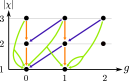
Figure 1: Dependency of the coefficients of the volume polynomials $V_{g,n}(\mathbf{x})$ when $|\chi|=2g-2+n\leq 3$. Note that all the coefficients for which $n\neq 0$ can therefore be computed thanks to the coefficients for which $|\chi|=1$.

Sequence $(u_{i})_{i}$ and first properties

In order to use the topological recursion formula stated in 2.1, we need some information of the sequence $(u_{i})_{i}$ that appears in it.

Lemma 2.2 ([Mir13, Lemma 3.1]).

The sequence $(u_{i})_{i}$ is increasing, converges to $1$ as $i$ approaches infinity, and there exists a constant $C>0$ such that

$$\forall i,\quad 0\leq u_{i+1}-u_{i}\leq\frac{C}{4^{i}}\cdot$$ (16)

We can deduce from the monotonicity of the sequence $(u_{i})_{i}$ the fact that the coefficients $(c_{g,n}(\alpha))_{\alpha}$ are decreasing functions of $\alpha$ in the following sense.

Lemma 2.3.

We define the following partial order on multi-indices:

$$\alpha\leq\tilde{\alpha}\quad\Leftrightarrow\quad\forall j\in\{1,\ldots,n\},\alpha_{j}\leq\tilde{\alpha}_{j}.$$

Then, the coefficients $(c_{g,n}(\alpha))_{\alpha}$ decrease with the multi-index $\alpha\in\mathbb{N}_{0}^{n}$. In particular,

$$\forall\alpha\in\mathbb{N}_{0}^{n},\quad 0\leq c_{g,n}(\alpha)\leq V_{g,n}.$$ (17)

Proof.

By symmetry of the coefficients, we can reduce the problem to proving that for any multi-indices $\alpha$ and $\tilde{\alpha}=(\tilde{\alpha}_{1},\alpha_{2},\ldots,\alpha_{n})$ such that $\tilde{\alpha}_{1}\geq\alpha_{1}$, $c_{g,n}(\tilde{\alpha})\leq c_{g,n}(\alpha)$. More precisely, we will show that every single term in equation 12 is smaller for the index $\tilde{\alpha}$ than it is for $\alpha$. The method being the same for every contribution, so we only detail the proof of the fact that $\mathcal{B}_{g,n}(\tilde{\alpha})\leq\mathcal{B}_{g,n}(\alpha)$. By equation 14, if we use the convention $u_{i}=0$ for $i<0$,

$$\mathcal{B}_{g,n}(\alpha)-\mathcal{B}_{g,n}(\tilde{\alpha})\\ =16\sum_{k_{1},k_{2}\geq 0}(\underbrace{u_{k_{1}+k_{2}+2-\alpha_{1}}-u_{k_{1}+k_{2}+2-\tilde{\alpha}_{1}}}_{\geq 0})\;c_{g-1,n+1}(k_{1},k_{2},\alpha_{2},\ldots,\alpha_{n})\geq 0.$$

∎

2.3 Estimates of ratios of Weil–Petersson volumes

Let us now review known estimates on ratios of Weil–Petersson volumes in the large-genus limit. These properties have been established in [Mir13] using several recursion formulas for Weil–Petersson volumes [Mir07a, DN09, LX09], amongst which the one presented in Section 2.2.

Same Euler characteristic

Since two surfaces with the same Euler characteristic are at the same height in the recursion formula, one could expect the volumes $V_{g,n}$ and $V_{g-1,n+2}$ to be of similar size. This is indeed the case: by [Mir13, Theorem 3.5], for all $n\geq 0$, there is a constant $C_{n}>0$ such that for any integer $g\geq 0$ satisfying $2g-2+n>0$,

$$\left|\frac{V_{g-1,n+2}}{V_{g,n}}-1\right|\leq\frac{C_{n}}{\langle g\rangle}\cdot$$ (18)

Adding a cusp

We can furthermore compare $V_{g,n}$ and $V_{g,n+1}$ using [Mir13, Lemma 3.2]: for any $g,n\geq 0$ such that $2g-2+n>0$,

$$\frac{1}{12}\left(1-\frac{\pi^{2}}{10}\right)<\frac{(2g-2+n)V_{g,n}}{V_{g,n+1}}<\frac{\pi\cosh(\pi)-\sinh(\pi)}{2\pi^{2}}\cdot$$ (19)

The fact that $V_{g,n+1}$ grows roughly like $(2g-2+n)V_{g,n}$ can be interpreted the following way: in order to sample a surface of signature $(g,n+1)$, we can start by sampling a surface of signature $(g,n)$. We then need to decide where to add a cusp, by picking a point on the surface of area proportional to $2g-2+n$.

Cutting into two smaller surfaces

Since we can cut surfaces of signature $(g,n)$ into two surfaces of respective signatures $(g_{1},n_{1}+1)$ and $(g_{2},n_{2}+1)$ with $g_{1}+g_{2}=g$ and $n_{1}+n_{2}=n$, one could expect the product $V_{g_{1},n_{1}+1}\times V_{g_{2},n_{2}+1}$ to be of similar size as $V_{g,n}$. Actually, these quantities are much smaller. Indeed, by [Mir13, Lemma 3.3], for any $n\geq 0$, there exists a constant $C_{n}>0$ satisfying the following. For any integer $g\geq 0$ such that $2g-2+n>0$ and any integers $n_{1}$, $n_{2}$ such that $n_{1}+n_{2}=n$,

$$\sum_{\begin{subarray}{c}g_{1}+g_{2}=g\\ 2g_{i}+n_{i}>1\end{subarray}}V_{g_{1},n_{1}+1}V_{g_{2},n_{2}+1}\leq C_{n}\frac{V_{g,n}}{\langle g\rangle}\cdot$$ (20)

The presence of this decay in $1/\langle g\rangle$ is linked to the fact that typical surfaces of large genus are very well-connected, and therefore quite difficult to cut into smaller pieces – a concrete manifestation of this phenomenon can be found in the comparison of Theorem 4.2 and Theorem 4.4 in [Mir13].

Cutting into more surfaces

In this article, we will need a new version of equation 20 with additional powers of the genus.

Lemma 2.4.

Let $n,N_{1},N_{2}\geq 0$ be integers. There exists a constant $C_{n,N_{1},N_{2}}$ satisfying the following. For any integer $g\geq 0$ such that $2g-2+n>0$ and any integers $n_{1}$, $n_{2}$ such that $n_{1}+n_{2}=n$,

$$\sum_{\begin{subarray}{c}g_{1}+g_{2}=g\\ 2g_{i}+n_{i}>N_{i}+1\end{subarray}}\frac{V_{g_{1},n_{1}+1}V_{g_{2},n_{2}+1}}{\langle g_{1}\rangle^{N_{1}}\langle g_{2}\rangle^{N_{2}}}\leq C_{n,N_{1},N_{2}}\frac{V_{g,n}}{\langle g\rangle^{N_{1}+N_{2}+1}}\cdot$$ (21)

We draw the reader’s attention to the fact that the sum is only taken over the set of indices $(g_{i},n_{i})$ such that $2g_{i}+n_{i}>N_{i}+1$. As we will see in the following proof, this is necessary and the result is false if we add a term with $1<2g_{i}+n_{i}\leq N_{i}+1$.

Proof.

The proof is an induction on the integer $N_{1}+N_{2}$, the case $N_{1}=N_{2}=0$ corresponding to equation 20.

Let $N_{1},N_{2}\geq 0$ such that $N:=N_{1}+N_{2}>0$. We assume the property at the rank $N-1$. By symmetry, we can assume that $N_{1}\geq N_{2}$, and in particular $N_{1}>0$. Then, for any $n_{1}$, $n_{2}$ such that $n_{1}+n_{2}=n$, the left hand side of equation 21 restricted to the terms where $g_{1}>0$ (which only exist if $g>0$) satisfies

$$\sum_{\begin{subarray}{c}g_{1}+g_{2}=g\\ 2g_{i}+n_{i}>N_{i}+1\\ g_{1}>0\end{subarray}}\frac{V_{g_{1},n_{1}+1}V_{g_{2},n_{2}+1}}{\langle g_{1}\rangle^{N_{1}}\langle g_{2}\rangle^{N_{2}}}=\mathcal{O}_{n_{1}}\Bigg{(}\sum_{\begin{subarray}{c}g_{1}^{\prime}+g_{2}=g-1\\ 2g_{1}^{\prime}+n_{1}^{\prime}>N_{1}\\ 2g_{2}+n_{2}>N_{2}+1\end{subarray}}\frac{V_{g_{1}^{\prime},n_{1}^{\prime}+1}V_{g_{2},n_{2}+1}}{\langle g_{1}\rangle^{N_{1}-1}\langle g_{2}\rangle^{N_{2}}}\Bigg{)}$$

since $V_{g_{1},n_{1}+1}/\langle g_{1}\rangle=\mathcal{O}_{n_{1}}(V_{g_{1}-1,n_{1}+2})$ by equations 18 and 19, and thanks to the change of indices $g_{1}^{\prime}=g_{1}-1$, $n_{1}^{\prime}=n_{1}+1$. By the induction hypothesis, this sum is

$$\mathcal{O}_{n+1,N_{1}-1,N_{2}}\left(\frac{V_{g-1,n+1}}{\langle g-1\rangle^{N}}\right)=\mathcal{O}_{n,N_{1},N_{2}}\left(\frac{V_{g,n}}{\langle g\rangle^{N+1}}\right)$$

by equations 18 and 19 again.

As a consequence, we are left to bound the term for which $g_{1}=0$. If such a term is present in the sum, then the integer $n_{1}=2g_{1}+n_{1}$ satisfies $n_{1}>N_{1}+1$, and hence $n-n_{2}-1\geq N_{1}+1$. Then, the term of the sum is

$$\frac{V_{0,n_{1}+1}V_{g,n_{2}+1}}{\langle 0\rangle^{N_{1}}\langle g\rangle^{N_{2}}}=\mathcal{O}_{n}\left(\frac{V_{g,n}}{\langle g\rangle^{N_{2}+n-n_{2}-1}}\right)=\mathcal{O}_{n}\left(\frac{V_{g,n}}{\langle g\rangle^{N+1}}\right)$$

by equation 19 applied $n-n_{2}-1$ times. ∎

2.4 The leading term of the asymptotic expansion

Let us conclude this preliminary section by a detailed proof of the following first-order estimate. This will allow us to present a few ideas that will be used in the general case.

Proposition 2.5 ([MP19, Proposition 3.1]).

For any $n\geq 1$, $g\geq 0$ such that $2g-2+n>0$, and any length vector $\mathbf{x}\in\mathbb{R}_{\geq 0}^{n}$,

$$\frac{V_{g,n}(\mathbf{x})}{V_{g,n}}=\prod_{j=1}^{n}\operatorname{sinhc}\left(\frac{x_{j}}{2}\right)+\mathcal{O}_{n}\left(\frac{|\mathbf{x}|}{\langle g\rangle}\exp\left(\frac{x_{1}+\ldots+x_{n}}{2}\right)\right).$$

This proposition comes as a consequence of the expression for the volume polynomials in terms of their coefficients $(c_{g,n}(\alpha))_{\alpha}$, together with the following first-order estimate for the coefficients.

Lemma 2.6.

For any $n\geq 1$, $g\geq 0$ such that $2g-2+n>0$, and any multi-index $\alpha\in\mathbb{N}_{0}^{n}$,

$$c_{g,n}(\alpha)=V_{g,n}+\mathcal{O}_{n}\left(|\alpha|^{2}\frac{V_{g,n}}{\langle g\rangle}\right).$$

Remark 2.7.

We insist on the fact that this estimate is true for any $\alpha$ and not only for multi-indices $\alpha$ such that $|\alpha|\leq 3g-3+n$. Indeed, if $|\alpha|>3g-3+n$, then the bound is trivial, because $c_{g,n}(\alpha)=0$ and $\frac{|\alpha|^{2}}{\langle g\rangle}\gg 1$.

We first prove 2.6 in Sections 2.4.1 and 2.4.2, and then deduce 2.5 from it in Section 2.4.3.

2.4.1 First-order estimate of the discrete derivative

2.6 states that the coefficients $c_{g,n}(\alpha)$ are almost constant, equal to the value $V_{g,n}=c_{g,n}(\mathbf{0}^{n})$. We will prove this by estimating the discrete derivatives of the coefficients $c_{g,n}(\alpha)$.

Lemma 2.8.

For any integers $g\geq 0$ and $n\geq 1$ satisfying $2g-2+n>0$, and any multi-index $\alpha\in\mathbb{N}_{0}^{n}$,

$$\delta_{1}c_{g,n}(\alpha)=\mathcal{O}_{n}\left(\langle\alpha\rangle\frac{V_{g,n}}{\langle g\rangle}\right).$$

Note that, by symmetry of the volume coefficients, this result is also true if we replace $\delta_{1}$ by $\delta_{i}$ for any $i\in\{1,\ldots,n\}$.

Proof.

The result is trivially true when $|\chi|=2g-2+n=1$, so we can assume that it is not the case and apply Mirzakhani’s topological recursion formula, 2.1:

$$\delta_{1}c_{g,n}(\alpha)=\sum_{j=2}^{n}\delta_{1}\mathcal{A}_{g,n}^{(j)}(\alpha)+\delta_{1}\mathcal{B}_{g,n}(\alpha)+\sum_{\iota\in\mathcal{I}_{g,n}}\delta_{1}\mathcal{C}_{g,n}^{(\iota)}(\alpha).$$

We prove that each of these three terms is $\mathcal{O}_{n}\left(\langle\alpha\rangle V_{g,n}/\langle g\rangle\right)$ separately thanks to their respective expressions, equations 13, 14 and 15.

Let us begin by the first sum. For a $j\geq 2$, we write equation 13 for $\mathcal{A}_{g,n}^{(j)}(\alpha)$ and $\mathcal{A}_{g,n}^{(j)}(\alpha_{1}+1,\alpha_{2},\ldots,\alpha_{n})$, isolating the term $i=0$ in the first sum and using a change of index on the sum over $i\geq 1$. We obtain

$$\delta_{1}\mathcal{A}_{g,n}^{(j)}(\alpha)= \;4\;(2\alpha_{j}+1)\;c_{g,n-1}(\alpha_{1}+\alpha_{j}-1,\alpha_{2},\ldots,\hat{\alpha}_{j},\ldots,\alpha_{n})$$

$$+8\;(2\alpha_{j}+1)\sum_{i=0}^{+\infty}(u_{i+1}-u_{i})\;c_{g,n-1}(i+\alpha_{1}+\alpha_{j},\alpha_{2},\ldots,\hat{\alpha}_{j},\ldots,\alpha_{n}).$$

But we know by 2.3 that for any multi-index $\beta\in\mathbb{N}_{0}^{n-1}$,

$$0\leq c_{g,n-1}(\beta)\leq V_{g,n-1}.$$

Then,

$$0\leq\delta_{1}\mathcal{A}_{g,n}^{(j)}(\alpha)\leq 8(2\alpha_{j}+1)V_{g,n-1}=\mathcal{O}_{n}\left(\langle\alpha_{j}\rangle\frac{V_{g,n}}{\langle g\rangle}\right)$$

because $\sum_{i=0}^{+\infty}(u_{i+1}-u_{i})=\lim u-u_{0}=1-\frac{1}{2}=\frac{1}{2}$ by 2.2, and thanks to equation 19. Since there are $n-1=\mathcal{O}_{n}\left(1\right)$ possible values for $j$,

$$\sum_{j=2}^{n}\delta_{1}\mathcal{A}_{g,n}^{(j)}(\alpha)=\mathcal{O}_{n}\left(\langle\alpha\rangle\frac{V_{g,n}}{\langle g\rangle}\right).$$ (22)

We now look at the non-separating term $\delta_{1}\mathcal{B}_{g,n}(\alpha)$. Note that this term only appears whenever $g\geq 1$. By the same method, this time applied to equation 14,

$$\delta_{1}\mathcal{B}_{g,n}(\alpha)= \,8\sum_{k_{1}+k_{2}=\alpha_{1}-2}c_{g-1,n+1}(k_{1},k_{2},\alpha_{2},\ldots,\alpha_{n})$$

$$+16\sum_{i=0}^{+\infty}\sum_{k_{1}+k_{2}=i+\alpha_{1}-1}(u_{i+1}-u_{i})\;c_{g-1,n+1}(k_{1},k_{2},\alpha_{2},\ldots,\alpha_{n})\cdot$$

By 2.3, for any multi-index $\beta\in\mathbb{N}_{0}^{n+1}$,

$$0\leq c_{g-1,n+1}(\beta)\leq V_{g-1,n+1}=\mathcal{O}_{n}\left(\frac{V_{g,n}}{\langle g\rangle}\right)$$

thanks to equations 19 and 18. Then,

$$\delta_{1}\mathcal{B}_{g,n}(\alpha)=\mathcal{O}_{n}\left(\alpha_{1}\frac{V_{g,n}}{\langle g\rangle}+\sum_{i=0}^{+\infty}(i+\alpha_{1})(u_{i+1}-u_{i})\frac{V_{g,n}}{\langle g\rangle}\right)=\mathcal{O}_{n}\left(\langle\alpha_{1}\rangle\frac{V_{g,n}}{\langle g\rangle}\right)$$ (23)

because the series $\sum_{i}(u_{i+1}-u_{i})$ and $\sum_{i}i(u_{i+1}-u_{i})$ converge.

Finally, for any configuration $\iota=(g^{\prime},I,J)\in\mathcal{I}_{g,n}$,

$$\delta_{1}\mathcal{C}_{g,n}^{(\iota)}(\alpha)= \,8\sum_{k_{1}+k_{2}=\alpha_{1}-2}c_{g^{\prime},|I|+1}(k_{1},\alpha_{I})\;c_{g-g^{\prime},|J|+1}(k_{2},\alpha_{J})$$

$$+16\sum_{i=0}^{+\infty}\sum_{k_{1}+k_{2}=i+\alpha_{1}-1}(u_{i+1}-u_{i})\;c_{g^{\prime},|I|+1}(k_{1},\alpha_{I})\;c_{g-g^{\prime},|J|+1}(k_{2},\alpha_{J})$$

$$= \,\mathcal{O}_{n}\left(\langle\alpha_{1}\rangle V_{g^{\prime},|I|+1}V_{g-g^{\prime},|J|+1}\right).$$

As a consequence,

$$\sum_{\iota\in\mathcal{I}_{g,n}}\delta_{1}\mathcal{C}_{g,n}^{(\iota)}(\alpha)=\mathcal{O}_{n}\Bigg{(}\langle\alpha_{1}\rangle\sum_{\begin{subarray}{c}g_{1}+g_{2}=g\\ n_{1}+n_{2}=n-1\\ 2g_{i}+n_{i}>1\end{subarray}}V_{g_{1},n_{1}+1}V_{g_{2},n_{2}+1}\Bigg{)}$$

and therefore, by equations 20 and 19,

$$\sum_{\iota\in\mathcal{I}_{g,n}}\delta_{1}\mathcal{C}_{g,n}^{(\iota)}(\alpha)=\mathcal{O}_{n}\left(\langle\alpha_{1}\rangle\frac{V_{g,n-1}}{\langle g\rangle}\right)=\mathcal{O}_{n}\left(\langle\alpha_{1}\rangle\frac{V_{g,n}}{\langle g\rangle^{2}}\right).$$ (24)

The conclusion follows from adding equations 22, 23 and 24. ∎

2.4.2 A discrete integration formula

In order to go from an estimate of discrete derivatives to an estimate on actual coefficients, we use the following discrete integration lemma.

Lemma 2.9.

Let $n\geq 1$ be an integer. For any $v:\mathbb{N}_{0}^{n}\rightarrow\mathbb{R}$,

$$v(\alpha)=v(\mathbf{0}^{n})-\sum_{i=1}^{n}\sum_{k=0}^{\alpha_{i}-1}\delta_{i}v(\mathbf{0}^{i-1},k,\alpha_{i+1},\ldots,\alpha_{n}).$$

2.6 then directly follows from this formula and our first-order estimate on the discrete derivatives, 2.8.

Proof of 2.9.

We observe that for any index $i$, the sum over $k$ is a telescopic sum:

$$S_{i} :=\sum_{k=0}^{\alpha_{i}-1}\delta_{i}v(\mathbf{0}^{i-1},k,\alpha_{i+1},\ldots,\alpha_{n})$$

$$=\sum_{k=0}^{\alpha_{i}-1}\left[v(\mathbf{0}^{i-1},k,\alpha_{i+1},\ldots,\alpha_{n})-v(\mathbf{0}^{i-1},k+1,\alpha_{i+1},\ldots,\alpha_{n})\right]$$

$$=v(\mathbf{0}^{i},\alpha_{i+1},\ldots,\alpha_{n})-v(\mathbf{0}^{i-1},\alpha_{i},\alpha_{i+1},\ldots,\alpha_{n}).$$

As a consequence, $\sum_{i=1}^{n}S_{i}=v(\mathbf{0}^{n})-v(\alpha)$, which what was claimed. ∎

2.4.3 From the coefficient estimate to the volume estimate

Let us finally prove that 2.6 implies 2.5.

Proof.

Using the expression of $\operatorname{sinhc}$ as a power series, we can write

$$V_{g,n}(\mathbf{x})-V_{g,n}\prod_{j=1}^{n}\operatorname{sinhc}\left(\frac{x_{j}}{2}\right)=\sum_{\begin{subarray}{c}\alpha\in\mathbb{N}_{0}^{n}\\ \alpha\neq\mathbf{0}^{n}\end{subarray}}(c_{g,n}(\alpha)-V_{g,n})\prod_{j=1}^{n}\frac{x_{j}^{2\alpha_{j}}}{2^{2\alpha_{j}}(2\alpha_{j}+1)!}\cdot$$

As a consequence, by the triangle inequality and 2.6,

$$\left|V_{g,n}(\mathbf{x})-V_{g,n}\prod_{j=1}^{n}\operatorname{sinhc}\left(\frac{x_{j}}{2}\right)\right|\leq C_{n}\frac{V_{g,n}}{\langle g\rangle}\sum_{\begin{subarray}{c}\alpha\in\mathbb{N}_{0}^{n}\\ \alpha\neq\mathbf{0}^{n}\end{subarray}}|\alpha|_{\infty}^{2}\prod_{j=1}^{n}\frac{x_{j}^{2\alpha_{j}}}{2^{2\alpha_{j}}(2\alpha_{j}+1)!}\cdot$$ (25)

We cut the sum over $\alpha$ in equation 25 depending on the index $j$ for which $|\alpha|_{\infty}=\alpha_{j}$. Since $\alpha_{j}^{2}\leq(2\alpha_{j}+1)(2\alpha_{j})/4$,

$$\sum_{\alpha_{j}=1}^{+\infty}\frac{\alpha_{j}^{2}\,x_{j}^{2\alpha_{j}}}{2^{2\alpha_{j}}(2\alpha_{j}+1)!}\leq\sum_{k=0}^{+\infty}\frac{x_{j}^{2k+2}}{2^{2k}(2k+1)!}=2x_{j}\sinh\left(\frac{x_{j}}{2}\right)\leq|\mathbf{x}|\exp\left(\frac{x_{j}}{2}\right).$$

Also, for any $i$,

$$\sum_{\alpha_{i}=0}^{+\infty}\frac{x_{i}^{2\alpha_{i}}}{2^{2\alpha_{i}}(2\alpha_{i}+1)!}\leq\sum_{k=0}^{+\infty}\frac{x_{i}^{k}}{2^{k}k!}\leq\exp\left(\frac{x_{i}}{2}\right).$$

This allows us to conclude. ∎

3 An explicit second-order expansion

We now possess all the tools that are required to compute the second term of the asymptotic expansion of $V_{g,n}(\mathbf{x})$. We recall the notation $\mathrm{c}(x)=\cosh\left(\frac{x}{2}\right)$ and $\mathrm{sc}(x)=\operatorname{sinhc}\left(\frac{x}{2}\right)$. Let us prove the following statement.

Theorem 3.1.

For any integers $g\geq 0$ and $n\geq 1$ such that $2g-2+n>0$, and any $\mathbf{x}\in\mathbb{R}_{\geq 0}^{n}$,

$$\frac{V_{g,n}(\mathbf{x})}{V_{g,n}}=F_{g,n}^{(1)}(\mathbf{x})+\mathcal{O}_{n}\left(\frac{\langle\mathbf{x}\rangle^{3}}{\langle g\rangle^{2}}\;\exp\left(\frac{x_{1}+\ldots+x_{n}}{2}\right)\right)$$

where the functions $F_{g,n}^{(1)}$ is the function defined by:

$$F_{g,n}^{(1)}(\mathbf{x})= \prod_{1\leq k\leq n}\mathrm{sc}(x_{k})$$

$$+8\;\frac{V_{g-1,n+1}\mathds{1}_{g\geq 1}}{V_{g,n}}\sum_{i=1}^{n}\left[\mathrm{c}(x_{i})+1-\left(\frac{x_{i}^{2}}{16}+2\right)\mathrm{sc}(x_{i})\right]\prod_{k\neq i}\mathrm{sc}(x_{k})$$

$$-4\;\frac{V_{g,n-1}}{V_{g,n}}\sum_{1\leq i<j\leq n}\left[\mathrm{c}(x_{i})\,\mathrm{c}(x_{j})+1-2\,\mathrm{sc}(x_{i})\,\mathrm{sc}(x_{j})\right]\prod_{k\notin\{i,j\}}\mathrm{sc}(x_{k}).$$

1.5 can then be obtained by using the expansions proved in [MZ15]: for any $g\geq 1$,

$$\frac{V_{g,n-1}}{V_{g,n}} =\frac{1}{8\pi^{2}g}+\mathcal{O}_{n}\left(\frac{1}{g^{2}}\right)$$

$$\frac{V_{g-1,n+1}}{V_{g,n}} =\frac{V_{g-1,n+1}}{V_{g,n-1}}\frac{V_{g,n-1}}{V_{g,n}}=\frac{1}{8\pi^{2}g}+\mathcal{O}_{n}\left(\frac{1}{g^{2}}\right).$$

The key ingredient in the proof of 3.1 is the following approximation result for the volume coefficients $(c_{g,n}(\alpha))_{\alpha}$ up to errors of size $V_{g,n}/\langle g\rangle^{2}$.

Proposition 3.2.

For any integers $g\geq 0$ and $n\geq 1$ such that $2g-2+n>0$,

$$\forall\alpha\in\mathbb{N}_{0}^{n},\quad c_{g,n}(\alpha)=\hat{c}_{g,n}^{(1)}(\alpha)+\mathcal{O}_{n}\left(|\alpha|^{4}\frac{V_{g,n}}{\langle g\rangle^{2}}\right)$$

where $\hat{c}_{g,n}^{(1)}:\mathbb{N}_{0}^{n}\rightarrow\mathbb{R}$ is the function defined by:

$$\hat{c}_{g,n}^{(1)}(\alpha)=V_{g,n} +8V_{g-1,n+1}\mathds{1}_{g\geq 1}\sum_{i=1}^{n}\left(p_{1}(\alpha_{i})+\mathds{1}_{\alpha_{i}=0}-\frac{p_{2}(\alpha_{i})}{4}-2\right)$$

$$-4V_{g,n-1}\mathds{1}_{n\geq 2}\sum_{1\leq i<j\leq n}\left(p_{1}(\alpha_{i})\,p_{1}(\alpha_{j})+\mathds{1}_{\alpha_{i}=\alpha_{j}=0}-2\right)$$

and $p_{1}(X):=2X+1$, $p_{2}(X):=(2X+1)(2X)$.

Similarly to the first-order case presented before, the proof of 3.2 spans over Sections 3.1 and 3.2, and we then deduce 3.1 from it in Section 3.3.

3.1 Second-order estimate of the discrete derivative

In order to expand the coefficients $(c_{g,n}(\alpha))_{\alpha\in\mathbb{N}_{0}^{n}}$, we first estimate the discrete derivative $\delta_{1}c_{g,n}(\alpha)$.

Lemma 3.3.

For any integers $g\geq 0$ and $n\geq 1$, satisfying $2g-2+n>0$,

$$\forall\alpha\in\mathbb{N}_{0}^{n},\quad\delta_{1}c_{g,n}(\alpha)=\psi_{g,n}^{(1)}(\alpha)+\mathcal{O}_{n}\left(\langle\alpha\rangle^{3}\frac{V_{g,n}}{\langle g\rangle^{2}}\right)$$

where $\psi_{g,n}^{(1)}:\mathbb{N}_{0}^{n}\rightarrow\mathbb{R}$ is the function defined by:

$$\psi_{g,n}^{(1)}(\alpha)= 4\,(4\alpha_{1}-1+2\,\mathds{1}_{\alpha_{1}=0})V_{g-1,n+1}\mathds{1}_{g\geq 1}$$

$$+4\sum_{j=2}^{n}(4\alpha_{j}+2-\mathds{1}_{\alpha_{1}=\alpha_{j}=0})V_{g,n-1}\mathds{1}_{n\geq 2}.$$

Proof.

We apply the discrete derivation to Mirzakhani’s recursion formula, 2.1:

$$\delta_{1}c_{g,n}(\alpha)=\sum_{j=2}^{n}\delta_{1}\mathcal{A}_{g,n}^{(j)}(\alpha)+\delta_{1}\mathcal{B}_{g,n}(\alpha)+\sum_{\iota\in\mathcal{I}_{g,n}}\delta_{1}\mathcal{C}_{g,n}^{(\iota)}(\alpha).$$

We then replace every term by the first-order approximation given by 2.6, which will allow us to estimate them up to errors of size $V_{g,n}/\langle g\rangle^{2}$.

We notice that the first term is zero if $n=1$. Let us assume otherwise, and take $j\in\{2,\ldots,n\}$. As in the first-order case, we can write

$$\delta_{1}\mathcal{A}_{g,n}^{(j)}(\alpha)= \;4\,(2\alpha_{j}+1)\;c_{g,n-1}(\alpha_{1}+\alpha_{j}-1,\alpha_{2},\ldots,\hat{\alpha}_{j},\ldots,\alpha_{n})$$

$$+8\,(2\alpha_{j}+1)\sum_{i=0}^{+\infty}(u_{i+1}-u_{i})\;c_{g,n-1}(i+\alpha_{1}+\alpha_{j},\alpha_{2},\ldots,\hat{\alpha}_{j},\ldots,\alpha_{n})$$

$$=: \;T_{1}+T_{2}.$$

• Estimate of the term $T_{1}$:

  • If $\alpha_{1}=\alpha_{j}=0$, then $\alpha_{1}+\alpha_{j}-1<0$ and therefore $T_{1}=0$.

  • Otherwise, by 2.6 applied to the coefficient in $T_{1}$,

    $$T_{1} =4\,(2\alpha_{j}+1)V_{g,n-1}+\mathcal{O}_{n}\left((2\alpha_{j}+1)|\alpha|^{2}\frac{V_{g,n-1}}{\langle g\rangle}\right)$$

    $$=4\,(2\alpha_{j}+1)V_{g,n-1}+\mathcal{O}_{n}\left(\langle\alpha\rangle^{3}\frac{V_{g,n}}{\langle g\rangle^{2}}\right)$$

    by equation 19.

• To estimate of the term $T_{2}$, we replace the volume coefficients appearing in $T_{2}$ by their first-order approximation and obtain:

  $$T_{2}=8\,(2\alpha_{j}+1)\sum_{i=0}^{+\infty}(u_{i+1}-u_{i})\left(V_{g,n-1}+\mathcal{O}_{n}\left((i+\left|\alpha\right|)^{2}\frac{V_{g,n-1}}{\langle g\rangle}\right)\right)$$

  by 2.6. But 2.2 implies that $\sum_{i=0}^{+\infty}(u_{i+1}-u_{i})=\frac{1}{2}$ and $\sum_{i=0}^{+\infty}i(u_{i+1}-u_{i})$ converges. Therefore, by equation 19 again,

  $$T_{2}=4\,(2\alpha_{j}+1)V_{g,n-1}+\mathcal{O}_{n}\left(\langle\alpha\rangle^{3}\frac{V_{g,n}}{\langle g\rangle^{2}}\right).$$

As a conclusion, we have proved that

$$\delta_{1}\mathcal{A}_{g,n}^{(j)}(\alpha)=\begin{cases}4\,V_{g,n-1}+\mathcal{O}_{n}\left(\langle\alpha\rangle^{3}\frac{V_{g,n}}{\langle g\rangle^{2}}\right)&\text{if }\alpha_{1}=\alpha_{j}=0\\ 8\,(2\alpha_{j}+1)V_{g,n-1}+\mathcal{O}_{n}\left(\langle\alpha\rangle^{3}\frac{V_{g,n}}{\langle g\rangle^{2}}\right)&\text{otherwise.}\end{cases}$$

We rewrite this expression as

$$\delta_{1}\mathcal{A}_{g,n}^{(j)}(\alpha)=4\,(4\alpha_{j}+2-\mathds{1}_{\alpha_{1}=\alpha_{j}=0})V_{g,n-1}\mathds{1}_{n\geq 2}+\mathcal{O}_{n}\left(\langle\alpha\rangle^{3}\frac{V_{g,n}}{\langle g\rangle^{2}}\right).$$

By the same process, we prove that, when $g\geq 1$,

$$\delta_{1}\mathcal{B}_{g,n}(\alpha)=4\,(4\alpha_{1}-1+2\,\mathds{1}_{\alpha_{1}=0})V_{g-1,n+1}\mathds{1}_{g\geq 1}+\mathcal{O}_{n}\left(\langle\alpha\rangle^{3}\frac{V_{g,n}}{\langle g\rangle^{2}}\right).$$

Indeed,

$$\delta_{1}\mathcal{B}_{g,n}(\alpha)= \,8\sum_{k_{1}+k_{2}=\alpha_{1}-2}c_{g-1,n+1}(k_{1},k_{2},\alpha_{2},\ldots,\alpha_{n})$$

$$+16\sum_{i=0}^{+\infty}\sum_{k_{1}+k_{2}=i+\alpha_{1}-1}(u_{i+1}-u_{i})\;c_{g-1,n+1}(k_{1},k_{2},\alpha_{2},\ldots,\alpha_{n})$$

$$=: \,T_{1}+T_{2}.$$

• On the one hand, $T_{1}$ is equal to zero if $\alpha_{1}=0$, and otherwise,

  $$T_{1}=8\,(\alpha_{1}-1)V_{g-1,n+1}+\mathcal{O}_{n}\left(\langle\alpha\rangle^{3}\frac{V_{g,n}}{\langle g\rangle^{2}}\right)$$

  because $V_{g-1,n+1}=\mathcal{O}_{n}\left(V_{g,n}/\langle g\rangle\right)$ by equations 19 and 18.

• On the other hand,

  $$T_{2} =16\sum_{i=0}^{+\infty}(\alpha_{1}+i)(u_{i+1}-u_{i})V_{g-1,n+1}+\mathcal{O}_{n}\left(\langle\alpha\rangle^{3}\frac{V_{g-1,n+1}}{\langle g-1\rangle}\right)$$

  $$=4\,(2\alpha_{1}+1)V_{g-1,n+1}+\mathcal{O}_{n}\left(\langle\alpha\rangle^{3}\frac{V_{g,n}}{\langle g\rangle^{2}}\right)$$

  because, as before, $\sum_{i=0}^{+\infty}(u_{i+1}-u_{i})=\frac{1}{2}$, and also $\sum_{i=0}^{+\infty}i(u_{i+1}-u_{i})=\frac{1}{4}$ by [MZ15, Lemma 2.1].

Finally, we observe that, when computing the first order term, we have proved in equation 24 that

$$\sum_{\iota\in\mathcal{I}_{g,n}}\delta_{1}\mathcal{C}_{g,n}^{(\iota)}(\alpha)=\mathcal{O}_{n}\left(\langle\alpha\rangle\frac{V_{g,n}}{\langle g\rangle^{2}}\right).$$

As a consequence, the separating term (C) does not contribute to the second-order approximation of $\delta_{1}c_{g,n}(\alpha)$.

Summing the different terms $\delta_{1}\mathcal{A}_{g,n}^{(j)}$ for $j\in\{2,\ldots,n\}$ and $\delta_{1}\mathcal{B}_{g,n}(\alpha)$ leads to the claim. ∎

3.2 Discrete integration of the second-order estimate

We can now prove 3.2 using 3.3 and discrete integration.

Proof.

By the discrete integration lemma (2.9) and by symmetry of the volume coefficients,

$$c_{g,n}(\alpha)=V_{g,n}-\sum_{i=1}^{n}\sum_{k=0}^{\alpha_{i}-1}\delta_{1}c_{g,n}(k,\mathbf{0}^{i-1},\alpha_{i+1},\ldots,\alpha_{n}).$$

We then apply 3.3 to deduce

$$c_{g,n}(\alpha)=V_{g,n}-\sum_{i=1}^{n}\sum_{k=0}^{\alpha_{i}-1}\psi^{(1)}_{g,n}(k,\mathbf{0}^{i-1},\alpha_{i+1},\ldots,\alpha_{n})+\mathcal{O}_{n}\left(\langle\alpha\rangle^{4}\frac{V_{g,n}}{\langle g\rangle^{2}}\right).$$

This can be rewritten as

$$c_{g,n}(\alpha)=V_{g,n}-4V_{g-1,n+1}\mathds{1}_{g\geq 1}T_{1}-4V_{g,n-1}\mathds{1}_{n\geq 2}T_{2}+\mathcal{O}_{n}\left(\langle\alpha\rangle^{4}\frac{V_{g,n}}{\langle g\rangle^{2}}\right)$$ (26)

where the quantities $T_{1}$ and $T_{2}$ are defined by

$$T_{1} :=\sum_{i=1}^{n}\sum_{k=0}^{\alpha_{i}-1}(4k-1+2\,\mathds{1}_{k=0})$$

$$T_{2} :=\sum_{i=1}^{n}\sum_{k=0}^{\alpha_{i}-1}\left[(i-1)(2-\mathds{1}_{k=0})+\sum_{j=i+1}^{n}(4\alpha_{j}+2-\mathds{1}_{k=\alpha_{j}=0})\right].$$

• On the one hand, we observe that for a fixed $i$, the term $\mathds{1}_{k=0}$ contributes to the sum at most once, and this occurs if and only if $\alpha_{i}>0$. Hence, when we perform the sum over $k$, we obtain

  $$T_{1}=\sum_{i=1}^{n}\left(2\alpha_{i}^{2}-3\alpha_{i}+2\,\mathds{1}_{\alpha_{i}>0}\right).$$

  We reorder the sum according to the dependency over $\alpha$, and use the fact that $\mathds{1}_{\alpha_{i}>0}=1-\mathds{1}_{\alpha_{i}=0}$, to obtain

  $$T_{1}=\sum_{i=1}^{n}\left(-2(2\alpha_{i}+1)-2\,\mathds{1}_{\alpha_{i}=0}+\frac{(2\alpha_{i}+1)(2\alpha_{i})}{2}+4\right).$$

• On the other hand, by the same method,

  $$T_{2} =\sum_{i=1}^{n}\left[(i-1)(2\alpha_{i}-\mathds{1}_{\alpha_{i}>0})+\sum_{j=i+1}^{n}(4\alpha_{i}\alpha_{j}+2\alpha_{i}-\mathds{1}_{\alpha_{i}>0}\mathds{1}_{\alpha_{j}=0})\right]$$

  $$=4\sum_{i<j}\alpha_{i}\alpha_{j}+2(n-1)\sum_{i=1}^{n}\alpha_{i}+\sum_{i>j}(\mathds{1}_{\alpha_{i}=0}-1)+\sum_{i<j}(\mathds{1}_{\alpha_{i}=0}-1)\mathds{1}_{\alpha_{j}=0}$$

  $$=\sum_{i<j}\left((2\alpha_{i}+1)(2\alpha_{j}+1)+\mathds{1}_{\alpha_{i}=\alpha_{j}=0}-2\right).$$

  This allows us to conclude, by equation 26.

∎

3.3 From the coefficient estimate to the volume estimate

In order to conclude the proof of 3.1, we need to compute

$$\sum_{\alpha\in\mathbb{N}_{0}^{n}}\hat{c}_{g,n}^{(1)}(\alpha)\prod_{j=1}^{n}\frac{x_{j}^{2\alpha_{j}}}{2^{2\alpha_{j}}(2\alpha_{j}+1)!}$$

where $\hat{c}^{(1)}_{g,n}(\alpha)$ is the approximation of the coefficient $c_{g,n}(\alpha)$ from 3.2. We have expressed $\hat{c}^{(1)}_{g,n}$ in terms of polynomials $p_{1}(X)=2X+1$ and $p_{2}(X)=(2X+1)(2X)$ in order to make this computation easier.

Since this will be useful for the general case, let us set some notations.

Notation.

For any integer $k\geq 0$, we set

$$p_{k}(X)=\prod_{j=0}^{k-1}(2X+1-j)=(2X+1)(2X)(2X-1)\ldots(2X+2-k),$$

with the convention that the empty product is equal to one so that $p_{0}(X)=1$.

Since the polynomials $(p_{k})_{k\geq 0}$ are a basis of the set of polynomials, we will be able to express any polynomial function as a linear combination of these polynomials. The following simple observation is our motivation for the introduction of these polynomials.

Lemma 3.4.

Let $k\geq 0$ be an integer. For any $x\in\mathbb{R}$,

$$\sum_{\alpha=0}^{+\infty}\frac{p_{k}(\alpha)\,x^{2\alpha}}{2^{2\alpha}(2\alpha+1)!}=\begin{cases}\frac{x^{k}}{2^{k}}\operatorname{sinhc}\left(\frac{x}{2}\right)&\text{if }k\text{ is even}\\ \frac{x^{k-1}}{2^{k-1}}\cosh\left(\frac{x}{2}\right)&\text{if }k\text{ is odd}.\end{cases}$$

We can now finish the proof of 3.1.

Proof.

By 3.2 and the expression of $V_{g,n}(\mathbf{x})$ in terms of $(c_{g,n}(\alpha))_{\alpha}$,

$$\frac{V_{g,n}(\mathbf{x})}{V_{g,n}}=F_{g,n}^{(1)}(\mathbf{x})+\mathcal{O}_{n}\left(\frac{V_{g,n}}{\langle g\rangle^{2}}\sum_{\begin{subarray}{c}\alpha\in\mathbb{N}_{0}^{n}\\ \alpha\neq\mathbf{0}^{n}\end{subarray}}|\alpha|_{\infty}^{4}\prod_{j=1}^{n}\frac{x_{j}^{2\alpha_{j}}}{2^{2\alpha_{j}}(2\alpha_{j}+1)!}\right)$$

where

$$F_{g,n}^{(1)}(\mathbf{x})=\sum_{\alpha\in\mathbb{N}_{0}^{n}}\frac{\hat{c}_{g,n}^{(1)}(\alpha)}{V_{g,n}}\prod_{j=1}^{n}\frac{x_{j}^{2\alpha_{j}}}{2^{2\alpha_{j}}(2\alpha_{j}+1)!}\cdot$$

We replace $\hat{c}_{g,n}^{(1)}$ by its expression from 3.2, and find the claimed expression by 3.4. The remainder is

$$\mathcal{O}_{n}\left(\frac{V_{g,n}}{\langle g\rangle^{2}}\langle\mathbf{x}\rangle^{3}\exp\left(\frac{x_{1}+\ldots+x_{n}}{2}\right)\right)$$

because for all $y\geq 0$,

$$\sum_{k=1}^{+\infty}\frac{k^{4}y^{2k}}{2^{2k}(2k+1)!}\leq y^{2}+\sum_{k=2}^{+\infty}\frac{p_{4}(k)\,y^{2k}}{2^{2k}(2k+1)!}=\mathcal{O}\left(\langle y\rangle^{3}\exp\left(\frac{y}{2}\right)\right).$$

∎

4 Proof of 1.3

The aim of this section is to prove 1.3, i.e. that for any order $N$,

$$\delta^{\mathbf{m}}c_{g,n}(\alpha)=\mathcal{O}_{n,N}\left(\langle\alpha\rangle^{N}\frac{V_{g,n}}{\langle g\rangle^{N}}\right),$$

for any $\mathbf{m}\in\mathbb{N}_{0}^{n}$ such that $|\mathbf{m}|\in\{2N-1,2N\}$ and any large enough multi-index $\alpha$. The proof relies on Mirzakhani’s recursion formula, 2.1. In order to be able to apply the discrete differential operator $\delta$ on its terms (14) and (15), we will use the following lemma.

Lemma 4.1.

Let $(c_{k_{1},k_{2}})_{k_{1},k_{2}\geq 0}$ be a family of real numbers, and $v:\mathbb{N}_{0}\rightarrow\mathbb{R}$ be the function defined by

$$\forall k\geq 0,\quad v_{k}:=\sum_{\begin{subarray}{c}k_{1}+k_{2}=k\\ k_{1},k_{2}\geq 0\end{subarray}}c_{k_{1},k_{2}}.$$

Then, for any integers $m\geq 1$ and $k\geq 0$,

$$\delta^{m}v_{k}=\sum_{\begin{subarray}{c}k_{1}+k_{2}=k\\ k_{1}\geq k_{2}\end{subarray}}\delta_{1}^{m}c_{k_{1},k_{2}}+\sum_{\begin{subarray}{c}k_{1}+k_{2}=k\\ k_{1}<k_{2}\end{subarray}}\delta_{2}^{m}c_{k_{1},k_{2}}-\sum_{m_{1}+m_{2}=m-1}\delta_{1}^{m_{1}}\delta_{2}^{m_{2}}c_{\lfloor\frac{k+1}{2}\rfloor,\lfloor\frac{k}{2}\rfloor+1}.$$

Proof.

We prove the formula by induction on the integer $m$. The initialisation at $m=0$ is trivial. For $m\geq 0$, let us assume the property at the rank $m$. Let $k\geq 0$ be an integer; we assume that $k=2p+1$ is an odd number (the proof when $k$ is even is the same). By definition of the operator $\delta$ and thanks to the induction hypothesis,

$$\delta^{m+1}v_{k}= \delta^{m}v_{k}-\delta^{m}v_{k+1}$$

$$= \sum_{\begin{subarray}{c}k_{1}+k_{2}=2p+1\\ k_{1}\geq k_{2}\end{subarray}}\delta_{1}^{m}c_{k_{1},k_{2}}-\sum_{\begin{subarray}{c}k_{1}+k_{2}=2p+2\\ k_{1}\geq k_{2}\end{subarray}}\delta_{1}^{m}c_{k_{1},k_{2}}$$

$$+\sum_{\begin{subarray}{c}k_{1}+k_{2}=2p+1\\ k_{1}<k_{2}\end{subarray}}\delta_{2}^{m}c_{k_{1},k_{2}}-\sum_{\begin{subarray}{c}k_{1}+k_{2}=2p+2\\ k_{1}<k_{2}\end{subarray}}\delta_{2}^{m}c_{k_{1},k_{2}}$$

$$-\sum_{m_{1}+m_{2}=m-1}(\delta_{1}^{m_{1}}\delta_{2}^{m_{2}}c_{p+1,p+1}-\delta_{1}^{m_{1}}\delta_{2}^{m_{2}}c_{p+1,p+2})$$

$$=: \,S_{1}-S_{2}+S_{3}-S_{4}-S_{5}.$$

Let us perform a change of indices $k_{1}^{\prime}=k_{1}-1$ in the sum $S_{2}$, singling out the term of $S_{2}$ for which $k_{1}=k_{2}=p+1$, so that we sum over the same set of indices as $S_{1}$. We obtain:

$$S_{1}-S_{2}=\Bigg{(}\sum_{\begin{subarray}{c}k_{1}+k_{2}=2p+1\\ k_{1}\geq k_{2}\end{subarray}}\delta_{1}^{m+1}c_{k_{1},k_{2}}\Bigg{)}-\delta_{1}^{m}c_{p+1,p+1}.$$

There is no boundary term when we do the same to $S_{3}$ and $S_{4}$, now changing the index $k_{2}$:

$$S_{3}-S_{4}=\sum_{\begin{subarray}{c}k_{1}+k_{2}=2p+1\\ k_{1}<k_{2}\end{subarray}}\delta_{2}^{m+1}c_{k_{1},k_{2}}.$$

We then observe that $\delta_{1}^{m}c_{p+1,p+1}+S_{5}$ is equal to

$$\delta_{1}^{m}c_{p+1,p+1}+\sum_{m_{1}+m_{2}=m-1}\delta_{1}^{m_{1}}\delta_{2}^{m_{2}+1}c_{p+1,p+1}=\sum_{m_{1}+m_{2}=m}\delta_{1}^{m_{1}}\delta_{2}^{m_{2}}c_{p+1,p+1}$$

which leads to the claimed expression for $\delta^{m+1}v_{k}$. ∎

We can now proceed to the proof of 1.3, which we restate here for convenience.

Theorem 4.2.

There exists an increasing sequence of integers $(a_{N})_{N\geq 0}$ satisfying the following. For any integers $g\geq 0$, $n\geq 1$ such that $2g-2+n>0$, any multi-indices $\mathbf{m},\alpha\in\mathbb{N}_{0}^{n}$ such that:

• $|\mathbf{m}|=m_{1}+\ldots+m_{n}\in\{2N-1,2N\}$

• $\forall i,(m_{i}\neq 0\Rightarrow\alpha_{i}\geq a_{N})$,

we have:

$$|\delta^{\mathbf{m}}c_{g,n}(\alpha)|\leq C_{n,N}\,\langle\alpha\rangle^{N}\frac{V_{g,n}}{\langle g\rangle^{N}}$$

where $C_{n,N}>0$ is a constant that depends only on $n$ and $N$.

Proof.

The proof is an induction on the integer $N$. The case $N=0$ is trivial: indeed, by Lemma 2.3,

$$\forall\alpha\in\mathbb{N}_{0}^{n},\quad|c_{\alpha}^{(g,n)}|\leq V_{g,n}.$$

In order to be able to use Mirzakhani’s recursion formula, we observe that the result is trivial when $2g-2+n=1$, for any $N>0$. Indeed,

• if $(g,n)=(0,3)$, then $\delta^{\mathbf{m}}c_{0,3}(\alpha)=0$ for any $\mathbf{m},\alpha\in\mathbb{N}_{0}^{3}$ such that $\alpha\neq\mathbf{0}^{3}$

• if $(g,n)=(1,1)$, then $\delta^{m}c_{1,1}(\alpha)=0$ for any $m\geq 0$ and any $\alpha\geq 2$.

As a consequence, provided that $a_{N}\geq 2$ for $N\geq 1$, the result is automatic.

For an integer $N\geq 0$, let us assume the result to hold at the rank $N$, and prove it at the rank $N+1$. Let us consider integers $g$, $n$ such that $2g-2+n>1$. Let $\mathbf{m},\alpha\in\mathbb{N}_{0}^{n}$ be multi-indices, such that:

• $|\mathbf{m}|=m_{1}+\ldots+m_{n}=2N+1$

• $\forall i,(m_{i}\neq 0\Rightarrow\alpha_{i}\geq a_{N+1})$,

where $a_{N+1}$ is an integer that will be determined during the proof. By symmetry of the volume coefficients, we can assume that $m_{1}>0$.

Let us write the coefficient $\delta^{\mathbf{m}}c_{\alpha}^{(g,n)}$ using Mirzakhani’s topological recursion formula, 2.1. We obtain:

$$|\delta^{\mathbf{m}}c_{g,n}(\alpha)| \leq\sum_{j=2}^{n}|\delta^{\mathbf{m}}\mathcal{A}^{(j)}_{g,n}(\alpha)|+|\delta^{\mathbf{m}}\mathcal{B}_{g,n}(\alpha)|+\sum_{\iota\in\mathcal{I}_{g,n}}|\delta^{\mathbf{m}}\mathcal{C}^{(\iota)}_{g,n}(\alpha)|$$

$$=:(A)+(B)+(C).$$

We shall estimate these different contributions successively, keeping in mind that the aim is to establish a decay for each term at the rate $\langle\alpha\rangle^{N+1}\frac{V_{g,n}}{\langle g\rangle^{N+1}}$.

Estimate of the term (A).

The term $(A)$ is equal to zero if $n=1$, and then there is nothing to be proved. Otherwise, let $j\in\{2,\ldots,n\}$. By equation 13,

$$\mathcal{A}^{(j)}_{g,n}(\alpha)=8\;(2\alpha_{j}+1)\sum_{i=0}^{+\infty}u_{i}\;c_{g,n-1}(\tilde{\alpha}^{(i)})$$

where $\tilde{\alpha}^{(i)}:=(i+\alpha_{1}+\alpha_{j}-1,\alpha_{2},\ldots,\hat{\alpha}_{j},\ldots,\alpha_{n})$. By a change of variable in the sum, if we set $u_{-1}=0$, then

$$\delta_{1}\mathcal{A}^{(j)}_{g,n}(\alpha)=8\;(2\alpha_{j}+1)\sum_{i=0}^{+\infty}(u_{i}-u_{i-1})\;c_{g,n-1}(\tilde{\alpha}^{(i)}).$$

• Let us first treat the case when $m_{j}=0$. By applying the discrete derivatives $\delta_{1}^{m_{1}-1}$ and $\delta_{i}^{m_{i}}$ for $i\notin\{1,j\}$, we observe that

  $$\delta^{\mathbf{m}}\mathcal{A}^{(j)}_{g,n}(\alpha)=8\;(2\alpha_{j}+1)\sum_{i=0}^{+\infty}(u_{i}-u_{i-1})\;\delta^{\tilde{\mathbf{m}}}c_{g,n-1}(\tilde{\alpha}^{(i)})$$

  for $\tilde{\mathbf{m}}=(m_{1}-1,m_{2},\ldots,\hat{m}_{j},\ldots,m_{n})$. Then, the bound on $u_{i}-u_{i-1}$ from 2.2 implies the existence of a universal constant $C>0$ such that

  $$|\delta^{\mathbf{m}}\mathcal{A}^{(j)}_{g,n}(\alpha)|\leq C\langle\alpha\rangle\sum_{i=0}^{+\infty}4^{-i}\;|\delta^{\tilde{\mathbf{m}}}c_{g,n-1}(\tilde{\alpha}^{(i)})|.$$

  We now want to use the induction hypothesis to bound $\delta^{\tilde{\mathbf{m}}}c_{g,n-1}(\tilde{\alpha}^{(i)})$, for every $i\geq 0$. We observe that $|\tilde{\mathbf{m}}|=|\mathbf{m}|-1=2N$, and decide to choose the parameter $a_{N+1}$ so that $a_{N+1}>a_{N}$. Then,

  $$i+\alpha_{1}+\alpha_{j}-1\geq\alpha_{1}-1\geq a_{N},$$

  and the multi-indices $\tilde{\mathbf{m}}$, $\tilde{\alpha}^{(i)}$ therefore satisfy the hypotheses of the theorem at the rank $N$. Hence,

  $$|\delta^{\tilde{\mathbf{m}}}c_{g,n-1}(\tilde{\alpha}^{(i)})|\leq C_{n-1,N}\,\langle\tilde{\alpha}^{(i)}\rangle^{N}\frac{V_{g,n-1}}{\langle g\rangle^{N}}\cdot$$

  By equation 19, this implies that

  $$\delta^{\tilde{\mathbf{m}}}c_{g,n-1}(\tilde{\alpha}^{(i)})=\mathcal{O}_{n,N}\left(\langle\alpha\rangle^{N}\langle i\rangle^{N}\frac{V_{g,n}}{\langle g\rangle^{N+1}}\right),$$

  from which we deduce that, as soon as $m_{j}=0$,

  $$|\delta^{\mathbf{m}}\mathcal{A}^{(j)}_{g,n}(\alpha)| =\mathcal{O}_{n,N}\left(\langle\alpha\rangle^{N+1}\frac{V_{g,n}}{\langle g\rangle^{N+1}}\sum_{i=0}^{+\infty}4^{-i}\langle i\rangle^{N}\right)$$

  $$=\mathcal{O}_{n,N}\left(\langle\alpha\rangle^{N+1}\frac{V_{g,n}}{\langle g\rangle^{N+1}}\right),$$

  which is precisely our claim.

• Now, if $m_{j}>0$, we need to be more careful when applying the derivative $\delta_{j}$ because of the dependance in $\alpha_{j}$ of $\mathcal{A}_{g,n}^{(j)}(\alpha)$. We prove by a simple induction that

  $$\delta^{\mathbf{m}}\mathcal{A}^{(j)}_{g,n}(\alpha)=\, 8\;(2\alpha_{j}+1)\sum_{i=0}^{+\infty}(u_{i}-u_{i-1})\;\delta^{\tilde{\mathbf{m}}}c_{g,n-1}(\tilde{\alpha}^{(i)})$$

  $$-16\,m_{j}\sum_{i=0}^{+\infty}(u_{i}-u_{i-1})\;\delta^{\hat{\mathbf{m}}}c_{g,n-1}(\tilde{\alpha}^{(i+1)})$$

  where $\tilde{\mathbf{m}}$ is as before and $\hat{\mathbf{m}}:=(m_{1}+m_{j}-2,m_{2},\ldots,\hat{m}_{j},\ldots,m_{n})$. We observe that $|\hat{\mathbf{m}}|=2N-1$, and this allows us to apply the induction hypothesis to this additional term. The same computation as in the case $m_{j}=0$ leads to the same bound, since $m_{j}=\mathcal{O}_{N}\left(1\right)$.

We sum up the $n-2=\mathcal{O}_{n}\left(1\right)$ contributions for $j\in\{2,\ldots,n\}$ and conclude that

$$\sum_{j=2}^{n}|\delta^{\mathbf{m}}\mathcal{A}^{(j)}_{g,n}(\alpha)|=\mathcal{O}_{n,N}\left(\langle\alpha\rangle^{N+1}\frac{V_{g,n}}{\langle g\rangle^{N+1}}\right).$$ (27)

∎

Estimate of the term (B).

Let us first observe that this term only appears whenever $g\geq 1$. As in the case (A), we start by writing that by equation 14,

$$\delta_{1}\mathcal{B}_{g,n}(\alpha)=16\sum_{i=0}^{+\infty}\sum_{k_{1}+k_{2}=i+\alpha_{1}-2}(u_{i}-u_{i-1})\;c_{g-1,n+1}(\tilde{\alpha}^{(k_{1},k_{2})})$$

where $\tilde{\alpha}^{(k_{1},k_{2})}=(k_{1},k_{2},\alpha_{2},\ldots,\alpha_{n})$. However, this time, the dependency on $\alpha_{1}$ is more complex, and we need to use 4.1 to apply the operator $\delta_{1}^{m_{1}-1}$ to the equation. We obtain:

$$|\delta^{\mathbf{m}}\mathcal{B}_{\alpha}^{(g,n)}|\leq \,C\sum_{i=0}^{+\infty}\sum_{\begin{subarray}{c}k_{1}+k_{2}=i+\alpha_{1}-2\\ k_{1}\geq k_{2}\end{subarray}}4^{-i}\;|\delta_{1}^{m_{1}-1}\delta^{\tilde{\mathbf{m}}}c_{g-1,n+1}(\tilde{\alpha}^{(k_{1},k_{2})})|$$ (28)

$$+C\sum_{i=0}^{+\infty}\sum_{\begin{subarray}{c}k_{1}+k_{2}=i+\alpha_{1}-2\\ k_{1}<k_{2}\end{subarray}}4^{-i}\;|\delta_{2}^{m_{1}-1}\delta^{\tilde{\mathbf{m}}}c_{g-1,n+1}(\tilde{\alpha}^{(k_{1},k_{2})})|$$ (29)

$$+C\sum_{\mu_{1}+\mu_{2}=m_{1}-2}\sum_{i=0}^{+\infty}4^{-i}|\delta_{1}^{\mu_{1}}\delta_{2}^{\mu_{2}}\delta^{\tilde{\mathbf{m}}}c_{g-1,n+1}(\tilde{\alpha}^{(\lfloor\frac{i+\alpha_{1}-1}{2}\rfloor,\lfloor\frac{i+\alpha_{1}}{2}\rfloor)})|,$$ (30)

where $\tilde{\mathbf{m}}=(0,0,m_{2},\ldots,m_{n})\in\mathbb{N}_{0}^{n+1}$, and the universal constant $C>0$ comes once again from 2.2. We estimate each term successively, using the induction hypothesis.

• Let us assume that the parameter $a_{N+1}$ is $\geq 2a_{N}+2$. Then, by hypothesis, $\alpha_{1}\geq 2a_{N}+2$, and therefore for any $i\geq 0$ and any $k_{1}$, $k_{2}$ in the $i$-th term of the sum (28),

  $$k_{1}\geq\frac{k_{1}+k_{2}}{2}=\frac{i+\alpha_{1}-2}{2}\geq a_{N}.$$

  We can then apply the induction hypothesis to $(m_{1}-1,\mathbf{0}^{n})+\tilde{\mathbf{m}}$, of $\ell^{1}$-norm $2N$, and $\tilde{\alpha}^{(k_{1},k_{2})}$. This yields

  $$|\delta_{1}^{m_{1}-1}\delta^{\tilde{\mathbf{m}}}c_{g-1,n+1}(\tilde{\alpha}^{(k_{1},k_{2})})| \leq C_{n+1,N}\,\langle\tilde{\alpha}^{(k_{1},k_{2})}\rangle^{N}\frac{V_{g-1,n+1}}{\langle g-1\rangle^{N}}$$

  $$=\mathcal{O}_{n,N}\left(\langle\tilde{\alpha}^{(k_{1},k_{2})}\rangle^{N}\frac{V_{g,n}}{\langle g\rangle^{N+1}}\right)$$

  since $g\geq 1$, and by equations 19 and 18. We then use the fact that

  $$\sum_{i=0}^{+\infty}\sum_{\begin{subarray}{c}k_{1}+k_{2}=i+\alpha_{1}-2\\ k_{1}\geq k_{2}\end{subarray}}4^{-i}\langle\tilde{\alpha}^{(k_{1},k_{2})}\rangle^{N}=\mathcal{O}_{N}\left(\langle\alpha\rangle^{N+1}\right),$$ (31)

  to conclude that if $a_{N+1}\geq 2a_{N}+2$, then the term (28) is

  $$\mathcal{O}_{n,N}\left(\langle\alpha\rangle^{N+1}\frac{V_{g,n}}{\langle g\rangle^{N+1}}\right).$$

• By symmetry of the coefficients, the term (29) is equal to

  $$\sum_{i=0}^{+\infty}\sum_{\begin{subarray}{c}k_{1}+k_{2}=i+\alpha_{1}-2\\ k_{2}>k_{1}\end{subarray}}4^{-i}\;|\delta_{1}^{m_{1}-1}\delta^{\tilde{\mathbf{m}}}c_{g-1,n+1}(\tilde{\alpha}^{(k_{2},k_{1})})|$$

  is therefore smaller than the term (28).

• For the term (30), we observe that since $\alpha_{1}\geq 2a_{N}+2$, for all $i\geq 0$,

  $$\left\lfloor\frac{i+\alpha_{1}}{2}\right\rfloor\geq\left\lfloor\frac{i+\alpha_{1}-1}{2}\right\rfloor\geq\frac{\alpha_{1}-2}{2}\geq a_{N}.$$

  Furthermore, for any integers such that $\mu_{1}+\mu_{2}=m_{1}-2$, the norm of $(\mu_{1},\mu_{2},\mathbf{0}^{n-1})+\tilde{\mathbf{m}}$ is equal to $2N-1$, and therefore, by the induction hypothesis,

  $$|\delta_{1}^{\mu_{1}}\delta_{2}^{\mu_{2}}\delta^{\tilde{\mathbf{m}}}c_{g-1,n+1}(\tilde{\alpha}^{(\lfloor\frac{i+\alpha_{1}-1}{2}\rfloor,\lfloor\frac{i+\alpha_{1}}{2}\rfloor)})|\\ \leq C_{n+1,N}\,\langle\tilde{\alpha}^{(\lfloor\frac{i+\alpha_{1}-1}{2}\rfloor,\lfloor\frac{i+\alpha_{1}}{2}\rfloor)}\rangle^{N}\frac{V_{g-1,n+1}}{\langle g-1\rangle^{N}},$$

  and (30) hence satisfies the same bound as the other terms.

As a conclusion, provided that $a_{N+1}\geq 2a_{N}+2$,

$$(B)=|\delta^{\mathbf{m}}\mathcal{B}_{g,n}(\alpha)|=\mathcal{O}_{n,N}\left(\langle\alpha\rangle^{N+1}\frac{V_{g,n}}{\langle g\rangle^{N+1}}\right).$$

∎

Estimate of the term (C).

For the term (C), similarly, by equation 15, for every configuration $\iota=(g_{1},I,J)$ where $g_{1}+g_{2}=g$ and $I\sqcup J=\{2,\ldots,n\}$, if we denote $n_{1}=|I|$ and $n_{2}=|J|$,

$$\delta_{1}\mathcal{C}^{(\iota)}_{g,n}(\alpha)=16\sum_{i=0}^{+\infty}\sum_{k_{1}+k_{2}=i+\alpha_{1}-2}(u_{i}-u_{i-1})\;c_{g_{1},n_{1}+1}(\tilde{\alpha}_{I}^{(k_{1})})\;c_{g_{2},n_{2}+1}(\tilde{\alpha}_{J}^{(k_{2})})$$

where $\tilde{\alpha}_{I}^{(k_{1})}=(k_{1},\alpha_{I})$ and $\tilde{\alpha}_{J}^{(k_{2})}=(k_{2},\alpha_{J})$. As before, we prove that

$$|\delta^{\mathbf{m}}\mathcal{C}^{(\iota)}_{g,n}(\alpha)|$$ (32)

$$\leq C\sum_{i=0}^{+\infty}\sum_{\begin{subarray}{c}k_{1}+k_{2}=\\ i+\alpha_{1}-2\\ k_{1}\geq k_{2}\end{subarray}}4^{-i}|\delta^{(m_{1}-1,\mathbf{m}_{I})}c_{g_{1},n_{1}+1}(\tilde{\alpha}_{I}^{(k_{1})})||\delta^{(0,\mathbf{m}_{J})}c_{g_{2},n_{2}+1}(\tilde{\alpha}_{J}^{(k_{2})})|$$ (33)

$$+C\sum_{i=0}^{+\infty}\sum_{\begin{subarray}{c}k_{1}+k_{2}=\\ i+\alpha_{1}-2\\ k_{1}<k_{2}\end{subarray}}4^{-i}|\delta^{(0,\mathbf{m}_{I})}c_{g_{1},n_{1}+1}(\tilde{\alpha}_{I}^{(k_{1})})||\delta^{(m_{1}-1,\mathbf{m}_{J})}c_{g_{2},n_{2}+1}(\tilde{\alpha}_{J}^{(k_{2})})|$$ (34)

$$+C\sum_{\begin{subarray}{c}\mu_{1}+\mu_{2}\\ =m_{1}-2\\ i\geq 0\end{subarray}}|\delta^{(\mu_{1},\mathbf{m}_{I})}c_{g_{1},n_{1}+1}(\tilde{\alpha}_{I}^{(\lfloor\frac{i+\alpha_{1}-1}{2}\rfloor)})||\delta^{(\mu_{2},\mathbf{m}_{J})}c_{g_{2},n_{2}+1}(\tilde{\alpha}_{I}^{(\lfloor\frac{i+\alpha_{1}}{2}\rfloor)})|.$$ (35)

We now estimate the term (33) using the induction hypothesis on the two terms $\delta^{(m_{1}-1,\mathbf{m}_{I})}c_{g_{1},n_{1}+1}(\tilde{\alpha}_{I}^{(k_{1})})$ and $\delta^{(0,\mathbf{m}_{J})}c_{g_{2},n_{2}+1}(\tilde{\alpha}_{J}^{(k_{2})})$. Let us set

$$N_{1}:=\left\lfloor\frac{m_{1}+|\mathbf{m}_{I}|}{2}\right\rfloor\leq N\quad\text{and}\quad N_{2}:=\left\lfloor\frac{|\mathbf{m}_{J}|+1}{2}\right\rfloor\leq N$$

so that $m_{1}-1+|\mathbf{m}_{I}|\in\{2N_{1}-1,2N_{1}\}$ and $|\mathbf{m}_{J}|\in\{2N_{2}-1,2N_{2}\}$. Then, we observe that under the hypothesis $a_{N+1}\geq 2a_{N}+2$, for any term in equation 33, $k_{1}\geq a_{N}\geq a_{N_{1}}$. We can therefore apply the induction hypothesis at the rank $N_{1}$ and obtain

$$\delta^{(m_{1}-1,\mathbf{m}_{I})}c_{g_{1},n_{1}+1}(\tilde{\alpha}_{I}^{(k_{1})})=\mathcal{O}_{n_{1},N_{1}}\left(\langle\tilde{\alpha}_{I}^{(k_{1})}\rangle^{N_{1}}\frac{V_{g_{1},n_{1}+1}}{\langle g_{1}\rangle^{N_{1}}}\right).$$

We also have that

$$\delta^{(0,\mathbf{m}_{J})}c_{g_{2},n_{2}+1}(\tilde{\alpha}_{J}^{(k_{2})})=\mathcal{O}_{n_{2},N_{2}}\left(\langle\tilde{\alpha}_{J}^{(k_{2})}\rangle^{N_{2}}\frac{V_{g_{2},n_{2}+1}}{\langle g_{2}\rangle^{N_{2}}}\right)$$

(note that there is no condition on the index $k_{2}$ because there is no derivative w.r.t. the first variable in $\delta^{(0,\mathbf{m}_{J})}$). We obtain by the same method as before that the term (33) is

$$\mathcal{O}_{n,N_{1},N_{2}}\left(\langle\alpha\rangle^{N_{1}+N_{2}+1}\frac{V_{g_{1},n_{1}+1}V_{g_{2},n_{2}+1}}{\langle g_{1}\rangle^{N_{1}}\langle g_{2}\rangle^{N_{2}}}\right).$$ (36)

We then wish to apply 2.4 in order to bound the sum over all configurations. This lemma implies that

$$\sum_{\begin{subarray}{c}\iota\in\mathcal{I}_{g,n}\\ 2g_{i}+n_{i}>N_{i}+1\end{subarray}}\frac{V_{g_{1},n_{1}+1}V_{g_{2},n_{2}+1}}{\langle g_{1}\rangle^{N_{1}}\langle g_{2}\rangle^{N_{2}}}=\mathcal{O}_{n,N}\left(\frac{V_{g,n-1}}{\langle g\rangle^{N_{1}+N_{2}+1}}\right)=\mathcal{O}_{n,N}\left(\frac{V_{g,n}}{\langle g\rangle^{N+2}}\right),$$ (37)

by equation 19 since $n_{1}+n_{2}=n-1$ for any $\iota\in\mathcal{I}_{g,n}$, and because

$$N_{1}+N_{2}=\left\lfloor\frac{m_{1}+|\mathbf{m}_{I}|}{2}\right\rfloor+\left\lfloor\frac{|\mathbf{m}_{J}|+1}{2}\right\rfloor\in\{N,N+1\}.$$

As a consequence, in order to conclude, we need to be able to restrict the sum over $\iota\in\mathcal{I}_{g,n}$ to the configurations such that $2g_{i}+n_{i}>N_{i}+1$ for $i\in\{1,2\}$. This is achieved by adding a new constraint on the parameter $a_{N+1}$: we assume that $a_{N+1}\geq 3(2N+1)$. Thanks to this additional hypothesis, we can prove that, for all configuration $\iota\in\mathcal{I}_{g,n}$,

• either $2g_{i}+n_{i}>N_{i}+1$ for $i=1$ and $2$;

• or $2g_{1}+n_{1}\leq N_{1}+1$, in which case $\delta^{(m_{1}-1,\mathbf{m}_{I})}c_{g_{1},n_{1}+1}(\tilde{\alpha}_{I}^{(k_{1})})=0$ for any integers $k_{1}\geq k_{2}$ such that $k_{1}+k_{2}\geq\alpha_{1}-2$;

• or $2g_{2}+n_{2}\leq N_{2}+1$, in which case $\delta^{(0,\mathbf{m}_{J})}c_{g_{2},n_{2}+1}(\tilde{\alpha}_{J}^{(k_{2})})=0$ for any integer $k_{2}\geq 0$.

Provided this claim is proved, we can then say that the sum over all configurations $\iota$ of the term (33) is equal to the sum over all $\iota$ such that $2g_{1}+n_{i}>N_{i}+1$, which then is

$$\mathcal{O}_{n,N}\left(\langle\alpha\rangle^{N+2}\frac{V_{g,n}}{\langle g\rangle^{N+2}}\right)$$

by equations 36 and 37. This implies that the sum (33) satisfies the claimed estimate for any $\alpha$ such that $|\alpha|\leq 3g-3+n$. Otherwise, because of the degree of $V_{g,n}(\mathbf{x})$, the sum (33) is equal to zero and the estimate trivially holds.

Let us now prove our claim.

• First, if $2g_{1}+n_{1}\leq N_{1}+1$, then for any $k_{1}\geq k_{2}$ such that $k_{1}+k_{2}\geq\alpha_{1}-2$, on the one hand,

  $$k_{1}+|\alpha_{I}| \geq\frac{k_{1}+k_{2}}{2}+\left|\alpha_{I}\right|\geq\frac{\alpha_{1}+\left|\alpha_{I}\right|}{2}-1$$

  $$\geq\frac{a_{N+1}}{2}\#\{i\in\{1\}\cup I\,:\,m_{i}\neq 0\}-1$$

  by hypothesis on $\alpha$. On the other hand,

  $$\#\{i\in\{1\}\cup I\,:\,m_{i}\neq 0\}\geq\frac{m_{1}+|\mathbf{m}_{I}|}{|\mathbf{m}|_{\infty}}\geq\frac{2N_{1}}{2N+1}\cdot$$

  We use the hypothesis $a_{N+1}\geq 3(2N+1)$ to deduce that

  $$k_{1}+|\alpha_{I}|\geq 3N_{1}-1\geq 6g_{1}+3n_{1}-4>3g_{1}-3+(n_{1}+1),$$

  because $3g_{1}+2n_{1}>2$. The latter quantity is the degree of the polynomial $V_{g_{1},n_{1}+1}(\mathbf{x})$ in the variables $x_{1}^{2},\ldots,x_{n_{1}+1}^{2}$, and therefore the previous inequality implies that $\delta^{(m_{1}-1,\mathbf{m}_{I})}c_{g_{1},n_{1}+1}(k_{1},\alpha_{I})=0$.

• Similarly, we prove that for any $k_{2}\geq 0$,

  $$k_{2}+|\alpha_{J}|\geq\frac{a_{N+1}|\mathbf{m}_{J}|}{|\mathbf{m}|_{\infty}}\geq 3(2N_{2}-1)$$

  and therefore if $2g_{2}+n_{2}\leq N_{2}+1$, then

  $$k_{2}+|\alpha_{J}|\geq 12g_{2}+6n_{2}-9>3g_{2}-3+(n_{2}+1)$$

  and hence $\delta^{(0,\mathbf{m}_{J})}c_{g_{2},n_{2}+1}(k_{2},\alpha_{J})=0$.

The estimate of the term (35) is the same: we apply the induction hypothesis to $\delta^{(\mu_{1},\mathbf{m}_{I})}c_{g_{1},n_{1}+1}(\tilde{\alpha}_{I}^{(\lfloor\frac{i+\alpha_{1}-1}{2}\rfloor)})$ and $\delta^{(\mu_{2},\mathbf{m}_{J})}c_{g_{2},n_{2}+1}(\tilde{\alpha}_{I}^{(\lfloor\frac{i+\alpha_{1}}{2}\rfloor)})$, at the admissible ranks

$$N_{1}:=\left\lfloor\frac{\mu_{1}+|\mathbf{m}_{I}|+1}{2}\right\rfloor\quad\text{and}\quad N_{2}:=\left\lfloor\frac{\mu_{2}+|\mathbf{m}_{J}|+1}{2}\right\rfloor.$$

We observe that $N_{1}+N_{2}=N$, and this therefore yields the claimed result. ∎

As a conclusion, we have proved that under the hypotheses $a_{N+1}\geq 2a_{N}+2$ and $a_{N+1}\geq 3(2N+1)$, for any multi-index $\mathbf{m}$ of norm $|\mathbf{m}|=2N+1$ and any multi-index $\alpha$ such that $\forall i,(m_{i}\neq 0\Rightarrow\alpha_{i}\geq a_{N+1})$,

$$|\delta^{\mathbf{m}}c_{g,n}(\alpha)|\leq(A)+(B)+(C)\leq C_{n,N+1}\,\langle\alpha\rangle^{N+1}\frac{V_{g,n}}{\langle g\rangle^{N+1}}\cdot$$

This implies the result for any multi-index $\mathbf{m}$ of norm $2N+2$ too, simply because for any sequence $(v(\alpha))_{\alpha}$, if $m_{1}>0$ for instance, then for all $\alpha$,

$$|\delta^{\mathbf{m}}v(\alpha)|\leq|\delta^{(m_{1}-1,m_{2},\ldots,m_{n})}v(\alpha)|+|\delta^{(m_{1}-1,m_{2},\ldots,m_{n})}v(\alpha_{1}+1,\alpha_{2},\ldots,\alpha_{n})|.$$

This concludes the induction. ∎

5 Proof of 1.1

5.1 Discrete Taylor expansion

1.3 states that the function $\alpha\mapsto c_{g,n}(\alpha)$ has small derivatives for large enough values of $\alpha$. Had we proved that the derivatives are small for any $\alpha$, we could have used a discrete version of the Taylor–Lagrange formula, such as the one below, to conclude that $\alpha\mapsto c_{g,n}(\alpha)$ is well-approximated by polynomial functions.

Lemma 5.1 (Discrete Taylor–Lagrange formula).

Let $n\geq 1$ and $f:\mathbb{N}_{0}^{n}\rightarrow\mathbb{R}$. We assume that there exist a real number $M\geq 0$ and integers $K,p\geq 0$ such that, for any multi-index $\mathbf{m}$ of norm $|\mathbf{m}|=K+1$,

$$\forall\alpha\in\mathbb{N}_{0}^{n},\quad|\delta^{\mathbf{m}}f(\alpha)|\leq M\langle\alpha\rangle^{p}.$$

Then, there exists a polynomial function $\tilde{f}^{(K)}:\mathbb{N}_{0}^{n}\rightarrow\mathbb{R}$ of degree at most $K$ such that

$$\forall\alpha\in\mathbb{N}_{0}^{n},\quad|f(\alpha)-\tilde{f}^{(K)}(\alpha)|\leq Mn^{K+1}\langle\alpha\rangle^{p+K+1}.$$

Furthermore, the coefficients of the polynomial function $\tilde{f}^{(K)}$ can be expressed as linear combinations of the derivatives $\delta^{\mathbf{m}}f(\mathbf{0}^{n})$, for multi-indices $\mathbf{m}\in\mathbb{N}_{0}^{n}$ of norm $|\mathbf{m}|\leq K$.

Proof.

We proceed by induction on the integer $K$.

For $K=0$, we observe that by 2.9, for all $\alpha$,

$$|f(\alpha)-f(\mathbf{0}^{n})|\leq\sum_{i=1}^{n}\sum_{k=0}^{\alpha_{i}-1}|\delta_{i}f(\mathbf{0}^{i-1},k,\alpha_{i+1},\ldots,\alpha_{n})|\leq Mn\langle\alpha\rangle^{p+1},$$

so the result holds if we take $\tilde{f}^{(0)}$ to be the constant function equal to $f(\mathbf{0}^{n})$.

Let us now assume the result at a rank $K-1$ for a $K\geq 1$, and deduce the result at the rank $K$. For any integer $i\in\{1,\ldots,n\}$, the function $\delta_{i}f$ satisfies the induction hypothesis at the rank $K-1$. Hence, there exists a polynomial function $\tilde{f}_{i}^{(K-1)}$ of degree at most $K-1$, and whose coefficients can be expressed as linear combinations of the $\delta^{\mathbf{m}}\delta_{i}f(\mathbf{0}^{n})$ for $|\mathbf{m}|\leq K-1$, such that

$$\forall\alpha\in\mathbb{N}_{0}^{n},\quad|\delta_{i}f(\alpha)-\tilde{f}_{i}^{(K-1)}(\alpha)|\leq Mn^{K}\langle\alpha\rangle^{p+K}.$$

Inspired by the discrete integration formula (2.9), we define

$$\tilde{f}^{(K)}(\alpha):=f(\mathbf{0}^{n})-\sum_{i=1}^{n}\sum_{k=0}^{\alpha_{i}-1}\tilde{f}_{i}^{(K-1)}(\mathbf{0}^{i-1},k,\alpha_{i+1},\ldots,\alpha_{n}).$$

We notice that $\tilde{f}^{(K)}$ is a polynomial of degree at most $K$, and its coefficients are linear combinations of $f(\mathbf{0}^{n})$ and the coefficients of $(\tilde{f}_{i})_{i}$, and therefore linear combinations of the $\delta^{\mathbf{m}}f(\mathbf{0}^{n})$ for $|\mathbf{m}|\leq K$. By 2.9, for any multi-index $\alpha\in\mathbb{N}_{0}^{n}$,

$$|f(\alpha)-\tilde{f}^{(K)}(\alpha)|$$

$$\leq\sum_{i=1}^{n}\sum_{k=0}^{\alpha_{i}-1}|\delta_{i}f(\mathbf{0}^{i-1},k,\alpha_{i+1},\ldots,\alpha_{n})-\tilde{f}_{i}^{(K-1)}(\mathbf{0}^{i-1},k,\alpha_{i+1},\ldots,\alpha_{n})|$$

$$\leq Mn^{K+1}\langle\alpha\rangle^{p+K+1},$$

and the conclusion follows. ∎

However, we can expect from the second-order approximation, 3.2, that the function $\alpha\in\mathbb{N}_{0}^{n}\mapsto c_{g,n}(\alpha)$ is not well-approximated by polynomial functions, but rather by a combination of polynomial functions and indicator functions, correcting the values of the function for small $\alpha$. The aim of the following section is to define such a class of functions, and prove a shifted Taylor–Lagrange estimate in this new setting.

5.2 Functions ultimately polynomial in each variable

Lemma 5.2 (and Definition).

For any integers $n\geq 1$ and $K,a\geq 0$, the two following families of functions $\mathbb{N}_{0}^{n}\rightarrow\mathbb{R}$,

• functions of the form

  $$\alpha\mapsto\prod_{i\in I}\alpha_{i}^{k_{i}}\,\prod_{i\notin I}\mathds{1}_{\alpha_{i}=\beta_{i}}$$

  where $I\subseteq\{1,\ldots,n\}$, $\mathbf{k}=(k_{i})_{i\in I}$ is a multi-index of norm $|\mathbf{k}|\leq K$, and $\beta=(\beta_{i})_{i\notin I}$ satisfies $|\beta|_{\infty}<a$;

• functions of the form

  $$\alpha\mapsto\prod_{i\in I}\alpha_{i}^{k_{i}}\mathds{1}_{\alpha_{i}\geq a}\,\prod_{i\notin I}\mathds{1}_{\alpha_{i}=\beta_{i}}$$

  where $I,\mathbf{k}$ and $\beta$ are defined the same way as in the first point;

generate the same linear subspace of the space of functions $\mathbb{N}_{0}^{n}\rightarrow\mathbb{R}$. We denote this space as $\mathcal{P}_{n,K,a}$, and call its elements polynomials (of degree at most $K$) in each variable greater than $a$.

Proof.

The equivalence of these two definitions comes from the simple observation that for any integers $a,\alpha\geq 0$,

$$1=\mathds{1}_{\alpha\geq a}+\sum_{\beta=0}^{a-1}\mathds{1}_{\alpha=\beta}.$$

∎

Then, elements of $\mathcal{P}_{n,K,a}$ are exactly the kind of functions we imagine the coefficients $\alpha\mapsto c_{g,n}(\alpha)$ to be well-approximated by: since the derivatives vanish for large enough $\alpha$, beyond a few small values, the functions are approximated by polynomials.

5.3 Shifted discrete Taylor expansion

Let us prove the following shifted Taylor–Lagrange lemma.

Lemma 5.3.

Let $n\geq 1$ be an integer and $f:\mathbb{N}_{0}^{n}\rightarrow\mathbb{R}$. We assume that there exists a real number $M\geq 0$ and integers $K,a,p\geq 0$ satisfying the following. For any multi-indices $\mathbf{m},\alpha\in\mathbb{N}_{0}^{n}$ such that:

• $|\mathbf{m}|=K+1$,

• $\forall i,(m_{i}\neq 0\Rightarrow\alpha_{i}\geq a)$,

we have

$$|\delta^{\mathbf{m}}f(\alpha)|\leq M\langle\alpha\rangle^{p}.$$

Then, there exists a function $\tilde{f}^{(K)}\in\mathcal{P}_{n,K,a}$ such that

$$\forall\alpha\in\mathbb{N}_{0}^{n},\quad|f(\alpha)-\tilde{f}^{(K)}(\alpha)|\leq C_{n,a,p,K}M\langle\alpha\rangle^{p+K+1}$$

where $C_{n,a,p,K}=2^{\frac{p}{2}+n}a^{n}\langle 2na\rangle^{p}n^{K+1}$. The coefficients of $\tilde{f}^{(K)}$ can be expressed as linear combinations of the values $\delta^{\mathbf{m}}f(\alpha)$ for multi-indices $\alpha,\mathbf{m}\in\mathbb{N}_{0}^{n}$ such that $|\alpha|_{\infty}\leq a$ and $|\mathbf{m}|\leq K$.

Proof.

The idea is to decompose $\mathbb{N}_{0}^{n}$ into subsets on which all of the variables are greater than $a$. More precisely, we notice that

$$1=\sum_{I\subset\{1,\ldots,n\}}\sum_{\begin{subarray}{c}(\beta_{i})_{i\notin I}\\ |\beta|_{\infty}<a\end{subarray}}\prod_{i\in I}\mathds{1}_{\alpha_{i}\geq a}\prod_{i\notin I}\mathds{1}_{\alpha_{i}=\beta_{i}}.$$

Then, we can rewrite the function $f$ as

$$f(\alpha)=\sum_{\begin{subarray}{c}I\subset\{1,\ldots,n\}\\ =\{i_{1}<\ldots<i_{r}\}\end{subarray}}\sum_{\begin{subarray}{c}(\beta_{i})_{i\notin I}\\ |\beta|_{\infty}<a\end{subarray}}g_{I,\beta}(\alpha_{i_{1}}-a,\ldots,\alpha_{i_{r}}-a)\prod_{i\in I}\mathds{1}_{\alpha_{i}\geq a}\prod_{i\notin I}\mathds{1}_{\alpha_{i}=\beta_{i}}$$ (38)

where $g_{I,\beta}:\mathbb{N}_{0}^{r}\rightarrow\mathbb{R}$ is defined by setting, for $\hat{\alpha}\in\mathbb{N}_{0}^{r}$, $g_{I,\beta}(\hat{\alpha}):=f(\alpha)$ where

$$\forall i,\alpha_{i}:=\begin{cases}\hat{\alpha}_{k}+a&\text{if }i=i_{k}\text{ for a }k\in\{1,\ldots,r\}\\ \beta_{i}&\text{if }i\notin I.\end{cases}$$

We wish to apply 5.1 to the function $g_{I,\beta}$. In order to do so, we need to prove an estimate on the derivatives $\delta^{\hat{\mathbf{m}}}g_{I,\beta}(\hat{\alpha})$ for any $\hat{\mathbf{m}},\hat{\alpha}\in\mathbb{N}_{0}^{r}$ such that $|\hat{\mathbf{m}}|=K+1$. This will follow from the hypothesis on the function $f$.

Indeed, we observe that, to any multi-index $\hat{\mathbf{m}}\in\mathbb{N}_{0}^{r}$ of norm $K+1$, we can associate a multi-index $\mathbf{m}\in\mathbb{N}_{0}^{n}$ also of norm $K+1$ by setting

$$\forall i,m_{i}:=\begin{cases}\hat{m}_{k}&\text{if }i=i_{k}\text{ for a }k\in\{1,\ldots,r\}\\ 0&\text{if }i\notin I.\end{cases}$$

Then, for any multi-indices $\hat{\mathbf{m}},\hat{\alpha}\in\mathbb{N}_{0}^{r}$, the corresponding multi-indices $\mathbf{m},\alpha$ automatically satisfy:

$$\forall i,(m_{i}\neq 0\Rightarrow i\in I\Rightarrow\alpha_{i}\geq a),$$

and therefore, by hypothesis on $f$,

$$|\delta^{\hat{\mathbf{m}}}g_{I,\beta}(\hat{\alpha})|=|\delta^{\mathbf{m}}f(\alpha)|\leq M\langle\alpha\rangle^{p}\leq M2^{\frac{p}{2}}\langle 2na\rangle^{p}\langle\hat{\alpha}\rangle^{p}$$

because $|\alpha|=|\hat{\alpha}|+ra+|\beta|\leq 2na+|\hat{\alpha}|$ and for any $x,y$, $\langle x+y\rangle\leq\sqrt{2}\langle x\rangle\langle y\rangle$.

We can therefore apply 5.1 to $g_{I,\beta}$, and deduce the existence of a polynomial $\tilde{g}_{I,\beta}^{(K)}$ in $r$ variables, of degree at most $K$, such that

$$\forall\hat{\alpha}\in\mathbb{N}_{0}^{r},\quad|g_{I,\beta}(\hat{\alpha})-\tilde{g}_{I,\beta}^{(K)}(\hat{\alpha})|\leq M2^{\frac{p}{2}}\langle 2na\rangle^{p}n^{K+1}\langle\hat{\alpha}\rangle^{p+K+1}.$$ (39)

Let us now define an element $\tilde{f}^{(K)}$ of $\mathcal{P}_{n,K,a}$ by the formula

$$\tilde{f}^{(K)}(\alpha):=\sum_{\begin{subarray}{c}I\subset\{1,\ldots,n\}\\ =\{i_{1}<\ldots<i_{r}\}\end{subarray}}\sum_{\begin{subarray}{c}(\beta_{i})_{i\notin I}\\ |\beta|_{\infty}<a\end{subarray}}\tilde{g}_{I,\beta}^{(K)}(\alpha_{i_{1}}-a,\ldots,\alpha_{i_{r}}-a)\prod_{i\in I}\mathds{1}_{\alpha_{i}\geq a}\prod_{i\notin I}\mathds{1}_{\alpha_{i}=\beta_{i}}.$$ (40)

By equations 38 and 40 together with the bound (39), for any $\alpha\in\mathbb{N}_{0}^{n}$,

$$|f(\alpha)-\tilde{f}^{(K)}(\alpha)|\leq M2^{\frac{p}{2}+n}a^{n}\langle 2na\rangle^{p}n^{K+1}\langle\alpha\rangle^{p+K+1}$$

because there are $2^{n}$ terms in the sum over the $I\subseteq\{1,\ldots,n\}$, and always less than $a^{n}$ possible choices for $\beta$. This is the claimed inequality.

The coefficients of $\tilde{f}^{(K)}$ are linear combinations of the coefficients of the $\tilde{g}_{I,\beta}^{(K)}$. By 5.1, these are themselves linear combinations of the values $\delta^{\hat{\mathbf{m}}}g_{I,\beta}(\mathbf{0}^{r})$ for multi-indices $\hat{\mathbf{m}}$ of norm $|\hat{\mathbf{m}}|\leq K$. By definition of $g_{I,\beta}$, these derivatives are derivatives of the form $\delta^{\mathbf{m}}f(\alpha)$ for multi-indices $\mathbf{m},\alpha$ such that $|\alpha|_{\infty}\leq a$ and $|\mathbf{m}|\leq K$. ∎

5.4 Proof of 1.1

We can now conclude with the proof of the asymptotic expansion, 1.1.

Proof.

Let $g\geq 0$, $n\geq 1$ be integers such that $2g-2+n>0$. Let $N\geq 0$ be a fixed order. By 1.3, there exists constants $C_{n,N+1},a_{N+1}$ such that

$$|\delta^{\mathbf{m}}c_{g,n}(\alpha)|\leq C_{n,N+1}\,\langle\alpha\rangle^{N+1}\frac{V_{g,n}}{\langle g\rangle^{N+1}}$$

for any multi-indices $\mathbf{m},\alpha\in\mathbb{N}_{0}^{n}$ such that

$$|\mathbf{m}|=2N+1\quad\text{and}\quad\forall i,(m_{i}\neq 0\Rightarrow\alpha_{i}\geq a_{N+1}).$$

This is exactly the hypothesis of 5.3, for the parameters $K:=2N$, $p:=N+1$, $a:=a_{N+1}$ and $M:=C_{n,N+1}V_{g,n}/\langle g\rangle^{N+1}$. As a consequence, there exists an element $\tilde{c}_{g,n}^{(K)}$ of $\mathcal{P}_{n,K,a}$ such that for all $\alpha\in\mathbb{N}_{0}^{n}$,

$$|c_{g,n}(\alpha)-\tilde{c}_{g,n}^{(K)}(\alpha)|\leq C_{n,a,p,K}\,M\langle\alpha\rangle^{p+K+1}$$

or, in other words,

$$c_{g,n}(\alpha)=\tilde{c}_{g,n}^{(2N)}(\alpha)+\mathcal{O}_{n,N}\left(\langle\alpha\rangle^{3N+2}\frac{V_{g,n}}{\langle g\rangle^{N+1}}\right).$$ (41)

Let us now define, for all $\mathbf{x}\in\mathbb{R}_{\geq 0}^{n}$, a good candidate for the approximating function,

$$F_{g,n}^{(N)}(\mathbf{x}):=\frac{1}{V_{g,n}}\sum_{\alpha\in\mathbb{N}_{0}^{n}}\tilde{c}^{(2N)}_{g,n}(\alpha)\prod_{i=1}^{n}\frac{x_{i}^{2\alpha_{i}}}{2^{2\alpha_{i}}(2\alpha_{i}+1)!}\cdot$$

Then, by equation 41 and the definition of $V_{g,n}(\mathbf{x})$ and $F_{g,n}^{(N)}(\mathbf{x})$,

$$\frac{V_{g,n}(\mathbf{x})}{V_{g,n}}=F_{g,n}^{(N)}(\mathbf{x})+\mathcal{O}_{n,N}\left(\sum_{\alpha\in\mathbb{N}_{0}^{n}}\frac{\langle\alpha\rangle^{3N+2}}{\langle g\rangle^{N+1}}\prod_{i=1}^{n}\frac{x_{i}^{2\alpha_{i}}}{2^{2\alpha_{i}}(2\alpha_{i}+1)!}\right).$$

We can control this remainder by writing that $\langle\alpha\rangle^{3N+2}=\mathcal{O}_{n,N}\left(1+|\alpha|_{\infty}^{3N+2}\right)$ and singling out an index $i$ such that $\alpha_{i}=|\alpha|_{\infty}$. Since, for any $D$, the polynomials $(p_{i})_{0\leq i\leq D}$ introduced in Notation are a basis of the set of polynomials of degree $\leq D$, we can express $\alpha_{i}^{3N+2}$ as a linear combination of $p_{k}(\alpha_{i})$ for integers $k\leq 3N+2$. Using 3.4, we obtain

$$\frac{V_{g,n}(\mathbf{x})}{V_{g,n}}=F_{g,n}^{(N)}(\mathbf{x})+\mathcal{O}_{n,N}\left(\frac{\langle\mathbf{x}\rangle^{3N+1}}{\langle g\rangle^{N+1}}\exp\left(\frac{x_{1}+\ldots+x_{n}}{2}\right)\right).$$

Let us now prove that $\mathbf{x}\mapsto F_{g,n}^{(N)}(\mathbf{x})$ has the claimed form. Note that by definition of the set $\mathcal{P}_{n,K,a}$, we can express the function $\alpha\mapsto\tilde{c}_{g,n}^{(K)}(\alpha)$ as a linear combination of functions of the form

$$g_{I,\beta,\mathbf{k}}(\alpha)=\prod_{i\in I}p_{k_{i}}(\alpha_{i})\prod_{i\notin I}\mathds{1}_{\alpha_{i}=\beta_{i}},$$

where $|\mathbf{k}|\leq K$ and $|\beta|_{\infty}<a_{N+1}$. By 3.4,

$$\sum_{\alpha\in\mathbb{N}_{0}^{n}}g_{I,\beta,\mathbf{k}}(\alpha)\prod_{i=1}^{n}\frac{x_{i}^{2\alpha_{i}}}{2^{2\alpha_{i}}(2\alpha_{i}+1)!}$$

$$=\prod_{\begin{subarray}{c}i\in I\\ k_{i}\text{ even}\end{subarray}}\frac{x_{i}^{k_{i}}}{2^{k_{i}}}\operatorname{sinhc}\left(\frac{x_{i}}{2}\right)\prod_{\begin{subarray}{c}i\in I\\ k_{i}\text{ odd}\end{subarray}}\frac{x_{i}^{k_{i}-1}}{2^{k_{i}-1}}\cosh\left(\frac{x_{i}}{2}\right)\prod_{\begin{subarray}{c}i\notin I\end{subarray}}\frac{x_{i}^{2\beta_{i}}}{2^{2\beta_{i}}(2\beta_{i}+1)!}\cdot$$

We therefore observe that $F_{g,n}^{(N)}$ is a linear combination of functions of the form

$$\mathbf{x}\mapsto x_{1}^{m_{1}}\ldots x_{n}^{m_{n}}\prod_{i\in I_{+}}\cosh\left(\frac{x_{i}}{2}\right)\prod_{i\in I_{-}}\operatorname{sinhc}\left(\frac{x_{i}}{2}\right)$$

where $I_{+}$ and $I_{-}$ are disjoint subsets of $\{1,\ldots,n\}$, and $\mathbf{m}=(m_{1},\ldots,m_{n})$ is a multi-index containing only even entries, which was our claim.

In order to bound the degree, we furthermore observe that

$$\sum_{i\in I_{+}}m_{i}+\sum_{i\in I_{-}}(m_{i}+1)\leq K=2N\quad\text{and}\quad\forall i\notin I_{+}\cup I_{-},m_{i}<a_{N+1}.$$

The coefficients are linear combinations of the derivatives $\delta^{\mathbf{m}}c_{g,n}(\alpha)/V_{g,n}$ for multi-indices $\mathbf{m},\alpha$ such that $|\mathbf{m}|\leq K$ and $|\alpha|_{\infty}\leq a_{N+1}$, which can therefore also be expressed in terms of the $c_{g,n}(\alpha)/V_{g,n}$ for $|\alpha|_{\infty}\leq a_{N+1}+2N$. ∎

We now conclude by proving how 1.1 implies 1.4.

Proof.

Let us first prove the existence of the asymptotic expansion. For any $I_{+}\sqcup I_{-}\subset\{1,\ldots,n\}$, the coefficients of the approximating polynomial $P_{g,n}^{(N,I_{\pm})}$ can be written as linear combinations of the $c_{g,n}(\alpha)/V_{g,n}$ with $|\alpha|_{\infty}\leq A_{N}$. By [MZ15, Theorem 4.1], for any such $\alpha$, we can write

$$\frac{c_{g,n}(\alpha)}{V_{g,n}}=\sum_{k=0}^{N}\frac{e_{n}^{(k)}(\alpha)}{g^{k}}+\mathcal{O}_{n,N}\left(\frac{1}{g^{N+1}}\right).$$

Note that the implied constant in the previous equation a priori depends on the multi-index $\alpha$, but since $|\alpha|_{\infty}\leq A_{N}$ we can bound it uniformly with a constant depending only on $N$. Then, $P_{g,n}^{(N,I_{\pm})}$ can be rewritten as

$$P_{g,n}^{(N,I_{\pm})}(\mathbf{x})=\sum_{k=0}^{N}\frac{\tilde{Q}_{n}^{(k,N,I_{\pm})}(\mathbf{x})}{g^{k}}+\mathcal{O}_{n,N}\left(\frac{\langle\mathbf{x}\rangle^{2N}}{g^{N+1}}\prod_{i\notin I_{+}\cup I_{-}}\langle x_{i}\rangle^{a_{N+1}}\right),$$ (42)

where $\tilde{Q}_{n}^{(k,N,I_{\pm})}$ are polynomial functions independent of $g$. The dependency of the remainder w.r.t. $\mathbf{x}$ in the previous expression is obtained by the bound on the degrees of $P_{g,n}^{(N,I_{\pm})}$ presented in 1.2. We then define, for each integer $k$, the function

$$\tilde{f}_{n}^{(k,N)}(\mathbf{x}):=\sum_{I_{+}\sqcup I_{-}\subset\{1,\ldots,n\}}\tilde{Q}_{n}^{(k,N,I_{\pm})}(\mathbf{x})\prod_{i\in I_{+}}\cosh\left(\frac{x_{i}}{2}\right)\prod_{i\in I_{-}}\operatorname{sinhc}\left(\frac{x_{i}}{2}\right).$$

Equations 2 and 42 together with the fact that

$$\prod_{i\notin I_{+}\sqcup I_{-}}x_{i}^{a_{N+1}}\prod_{i\in I_{+}}\cosh\left(\frac{x_{i}}{2}\right)\prod_{i\in I_{-}}\sinh\left(\frac{x_{i}}{2}\right)=\mathcal{O}_{N,n}\left(\exp\left(\frac{x_{1}+\ldots+x_{n}}{2}\right)\right)$$

imply that these approximating functions satisfy (5), i.e. for all $\mathbf{x}\in\mathbb{R}_{\geq 0}^{n}$,

$$\frac{V_{g,n}(\mathbf{x})}{V_{g,n}}=\sum_{k=0}^{N}\frac{\tilde{f}_{n}^{(k,N)}(\mathbf{x})}{g^{k}}+\mathcal{O}_{N,n}\left(\frac{\langle\mathbf{x}\rangle^{3N+1}}{g^{N+1}}\exp\left(\frac{x_{1}+\ldots+x_{n}}{2}\right)\right).$$

We now observe that, for any fixed $\mathbf{x}$, the previous equation is an asymptotic expansion of $V_{g,n}(\mathbf{x})/V_{g,n}$ in powers of $g$, and its coefficients are therefore uniquely defined. In particular, for any $N^{\prime}<N$ and any $k\in\{0,\ldots,N^{\prime}\}$, $\tilde{f}_{n}^{(k,N)}(\mathbf{x})=\tilde{f}_{n}^{(k,N^{\prime})}(\mathbf{x})$, and the number $\tilde{f}_{n}^{(k,N)}(\mathbf{x})$ does not depend on the order of approximation $N$ and can be denoted more simply as $f_{n}^{(k)}(\mathbf{x})$.

Finally, the decomposition (6) of $f_{n}^{(k)}$ is uniquely defined because the family of functions of the form

$$\mathbf{x}\in\mathbb{R}_{\geq 0}^{n}\mapsto x_{1}^{m_{1}}\ldots x_{n}^{m_{n}}\prod_{i\in I_{+}}\cosh\left(\frac{x_{i}}{2}\right)\prod_{i\in I_{-}}\operatorname{sinhc}\left(\frac{x_{i}}{2}\right)$$

for $m_{1},\ldots,m_{n}\geq 0$ and $I_{+}\sqcup I_{-}\subseteq\{1,\ldots,n\}$ is free. ∎

References

- [Bus92] Peter Buser. Geometry and Spectra of Compact Riemann Surfaces. Birkhäuser, Boston, 1992.
- [Che75] Shiu-Yuen Cheng. Eigenvalue comparison theorems and its geometric applications. Mathematische Zeitschrift, 143(3):289–297, 1975.
- [DN09] Norman Do and Paul Norbury. Weil–Petersson volumes and cone surfaces. Geometriae Dedicata, 141:93–107, 2009.
- [Gol84] William M. Goldman. The symplectic nature of fundamental groups of surfaces. Advances in Mathematics, 54(2):200–225, 1984.
- [GPY11] Larry Guth, Hugo Parlier, and Robert Young. Pants decompositions of random surfaces. Geometric and Functional Analysis, 21(5):1069–1090, 2011.
- [HM21] Will Hide and Michael Magee. Near optimal spectral gaps for hyperbolic surfaces. arXiv:2107.05292, 2021.
- [LW21] Michael Lipnowski and Alex Wright. Towards optimal spectral gaps in large genus. arXiv:2103.07496, 2021.
- [LX09] Kefeng Liu and Hao Xu. Recursion formulae of higher Weil–Petersson volumes. International Mathematics Research Notices, 5:835–859, 2009.
- [Mir07a] Maryam Mirzakhani. Simple geodesics and Weil–Petersson volumes of moduli spaces of bordered Riemann surfaces. Inventiones Mathematicae, 167(1):179–222, 2007.
- [Mir07b] Maryam Mirzakhani. Weil–Petersson volumes and intersection theory on the moduli space of curves. Journal of the American Mathematical Society, 20(1):1–23, 2007.
- [Mir13] Maryam Mirzakhani. Growth of Weil–Petersson volumes and random hyperbolic surfaces of large genus. Journal of Differential Geometry, 94(2):267–300, 2013.
- [Mon21] Laura Monk. Geometry and Spectrum of Typical Hyperbolic Surfaces. PhD thesis, Université de Strasbourg, 2021.
- [MP19] Maryam Mirzakhani and Bram Petri. Lengths of closed geodesics on random surfaces of large genus. Commentarii Mathematici Helvetici, 94(4):869–889, 2019.
- [MT21] Laura Monk and Joe Thomas. The tangle-free hypothesis on random hyperbolic surfaces. International Mathematics Research Notices, rnab160, 2021.
- [MZ15] Maryam Mirzakhani and Peter Zograf. Towards large genus asymptotics of intersection numbers on moduli spaces of curves. Geometric and Functional Analysis, 25(4):1258–1289, 2015.
- [NN98] Marjatta Näätänen and Toshihiro Nakanishi. Weil–Petersson areas of the moduli spaces of tori. Results in Mathematics, 33(1-2):120–133, 1998.
- [NWX20] Xin Nie, Yunhui Wu, and Yuhao Xue. Large genus asymptotics for lengths of separating closed geodesics on random surfaces. arXiv:2009.07538, 2020.
- [Wei58] André Weil. On the moduli of Riemann surfaces. In Œuvres Scientifiques - Collected Papers II:1951-1964, pages 379–389. Springer-Verlag, Berlin, Heidelberg, 1958.
- [WX21] Yunhui Wu and Yuhao Xue. Random hyperbolic surfaces of large genus have first eigenvalues greater than . arXiv:2102.05581, 2021.