Large-time asymptotics of the wave fronts length I
The Euclidean disk

In the paper [Vi-20], the second author proves that the length $|S_{t}|$ of the wave front $S_{t}$ at time $t$ of a wave propagating in an Euclidean disk ${\mathbb{D}}$ of radius $1$, starting from a source $q$, admits a linear asymptotics as $t\rightarrow+\infty$: $|S_{t}|=\lambda(q)t+\mathrm{o}(t)$ with $\lambda(q)=2\arcsin a$ and $a=d(0,q)$. We will give a more direct proof and compute the oscillating corrections to this linear asymptotics. The proof is based on the “stationary phase” approximation.

1 Wave fronts

Let us consider a 2D-Riemannian compact manifold $(X,g)$ possibly with a smooth convex boundary. We denote by $g^{\star}:T^{\star}X\rightarrow{\mathbb{R}}$ the half of the dual metric which is the Hamiltonian of the geodesic flow.

We denote by $\pi_{X}$ the canonical projection of $T^{\star}X$ onto $X$ and $\phi_{t}:T^{\star}X\rightarrow T^{\star}X,~{}t\in{\mathbb{R}}$ the Hamiltonian flow of $g^{\star}$ which is the geodesic flow. If $X$ has a non empty boundary, we define $\phi_{t}$ using the law of reflection. Let $q\in X$ be given. For any $t>0$, we define the wave front $S_{t}$ at time $t$ as the set of points of $X$ of the form $\pi_{X}(\phi_{t}(\Sigma^{q}))$ where $\Sigma^{q}:=\{(q,\xi)\in T^{\star}X|g^{\star}(q,\xi)=1\}$. The set $S_{t}$ could also be defined as the image by the exponential map at $q$ of the circle $\Sigma_{t}$ of radius $t$ in the tangent space $T_{q}X$.

Let us define the length of $S_{t}$ and denote it by $|S_{t}|$. The wave front $S_{t}$ is a curve parametrized by a circle: $S_{t}:={\rm exp}_{q}(\Sigma_{t})$. This allows to define its length using the Riemannian metric. Note that $S_{t}$ can admit some singular points. The length of the corresponding part vanishes and the remaining part is an immersed co-oriented curve with only transversal self-intersections.

In this article, we focus on the case where $X$ is the unit disk in $\mathbb{R}^{2}$ and $g$ is the Euclidean metric. In this context, we will prove that the following expansion holds:

$$|S_{t}|=2\alpha_{0}t+t\sum_{n=0}^{\infty}J_{n}^{\rm approx}(t)+\mathrm{O}(1)$$ (1)

as $t\to+\infty$, with

$$J_{n}^{\rm approx}(t)=\frac{-8\sqrt{2}}{\pi^{2}(2n+1)^{5/2}\sqrt{t}}\cos\left((2n+1)\pi a\right)\cos\left(\pi\left((2n+1)t+\frac{1}{4}\right)\right)$$

where $a$ is the distance from the point $q$ to the center of the disk.

The case of closed surfaces with integrable geodesic flows will be the subject of [CV-20].

2 Numerics

In this section, we will compare the expansion given by $(\ref{resultat_principal})$ with the numerical calculations. We introduce a (small) time step $\delta_{t}>0$, a (large) number of points $n$ which compose the wave front, two vectors $M$ and $V$ in $(\mathbb{R}^{2})^{n}$ such that, for any $k\in[\![1,n]\!]$, $X_{k}\in\mathbb{R}^{2}$ represents the position and $V_{k}\in\mathbb{R}^{2}$ the speed of the $k$th point of the wave front at a given time. We fix $a\in]0,1[$ such that $(a,0)$ are the coordinates of the source $q$. Thus, we introduce the following iterative scheme

$${}\left\{\begin{array}[]{l}\mbox{{initialization:}}\\ \begin{array}[]{l}M\leftarrow\left((a,0),\ldots,(a,0)\right)\in(\mathbb{R}^{2})^{n},\\ \mbox{for any }k\in[\![1,n]\!],V_{k}\leftarrow\left(\cos\left(\frac{2k\pi}{n}\right),\sin\left(\frac{2k\pi}{n}\right)\right),\\ \end{array}\\ \mbox{{iterative step:}}\\ \begin{array}[]{l}\widetilde{M}\leftarrow M+\delta_{t}V,\\ \mbox{for any $k\in[\![1,n]\!]$, }\left\{\begin{array}[]{l}\mbox{ if }{\widetilde{M}}_{k}\in\mathbb{D}\mbox{ then }M_{k}\leftarrow{\widetilde{M}}_{k},\\ \mbox{ else }\\ \mbox{ }\quad\mbox{compute }{\delta_{t}^{k}}\mbox{ s.t. }\|M_{k}+{\delta_{t}^{k}}V_{k}\|=1\mbox{ and }{\delta_{t}^{k}}\geq 0,\\ \mbox{ }\quad M_{k}\leftarrow M_{k}+\delta_{t}^{k}V_{k},\\ \mbox{ }\quad V_{k}\leftarrow V_{k}-2\left<V_{k}|\frac{M_{k}}{\|M_{k}\|}\right>\frac{M_{k}}{\|M_{k}\|},\\ \mbox{ }\quad M_{k}\leftarrow M_{k}+(\delta_{t}-\delta_{t}^{k})V_{k}.\end{array}\right.\\ \end{array}\end{array}\right.$$

The iterative loop consists in the computation of a linear motion outside the boundary and at the boundary one applies the familiar law the angle of incidence equals the angle of reflection. After $p$ iterations, $M$ represents the points of the wave front (see Figure 1 and Videos).

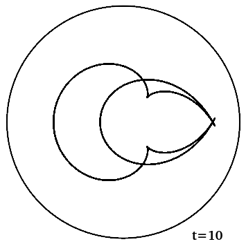
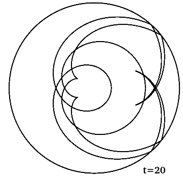
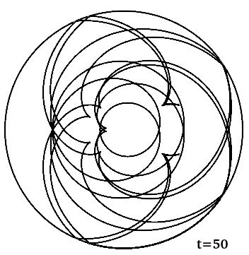
Figure 1: Wave Front for $a=0.5$ and $t\in\{0.5,10,20,50\}$

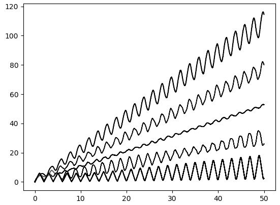
Figure 2: Length of the wave front $|S_{t}|$ for $t\in[0,50]$ and for differents values of $a$, respectively (from bottom to top), for $a=0.1$, $a=0.3$, $a=0.5$, $a=0.7$ and $a=0.9$

First, we can observe that $|S_{t}|$ admits a linear asymptotic as $t$ grows to $+\infty$. Then, the oscillations are of period 2 with a phase independent of $a$ (see Figure 2). One may remark the following points.

1. For $a=0$, the family of curves $(S_{t})_{t}$ are concentric circles and $|S_{t}|$ is of period 2.

2. For $a=0.5$, the terms $J_{k}^{\rm approx}(t)$ vanish for any $t$ and, in this case, this expansion is not able to capture the oscillating part of $t\mapsto|S_{t}|$.

3. The terms $|J_{k}^{\rm approx}(t)|$ are bounded by $Ck^{-5/2}t^{-1/2}$, where $C$ is a constant. For $t$ fixed, this ensures the (fast) convergence of the serie $\sum_{k}J_{k}^{\rm approx}(t)$ and then the amplitude of $\displaystyle t\mapsto t\sum_{k\in{\mathbb{N}}}J_{k}^{\rm approx}(t)$ is of order $t^{1/2}$ (see Figure 3).

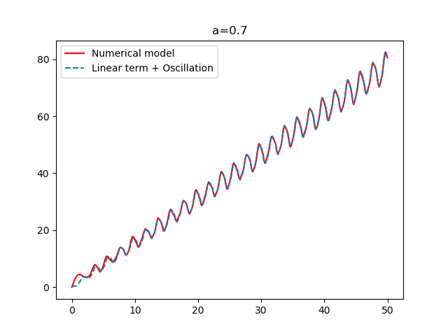
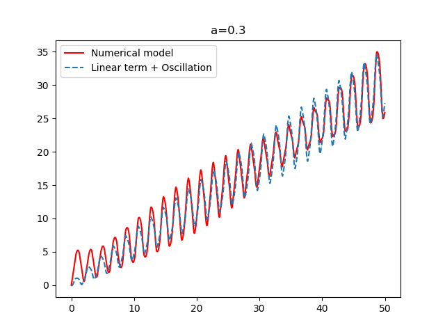
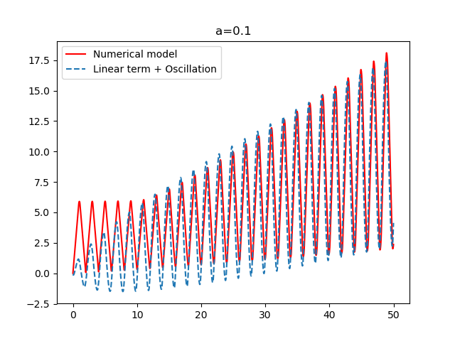
Figure 3: Comparison between $|S_{t}|$ and $2\arcsin(a)t+t\sum_{k=0}^{N}J_{k}^{\rm approx}(t)$ for $N=10$, $t\in[0,50]$ and $a\in\{0.1,0.3,0.7,0.9\}$.

3 A short proof of the Arcsinus formula

In the paper [Vi-20], the author was able to prove by elementary calculations the

Theorem 3.1

If $X$ is the unit disk, $|S_{t}|=\lambda(q)t+\mathrm{o}(t)$ as $t\to+\infty$ with radius $1$ with $\lambda(q)=2\arcsin a$ where $a$ is the distance from $q$ to the center of the disk.

We will reprove it using tools which will be extended to integrable geodesic flows in a forthcoming paper. For this, we will prove an integral formula:

Theorem 3.2

Let $\psi$ be the function periodic of period $1$ whose restriction to $[0,1]$ is given by $\psi(\theta)=|2\theta-1|$. We have

$$|S_{t}|=t\Sigma_{\pm}\int_{I_{\alpha_{0}}}\psi\left(\theta_{2}^{\pm,q}(\xi)-\frac{t}{2\sin\xi}\right)d\xi+\mathrm{O}(1)$$ (2)

as $t\to+\infty$, where $I_{\alpha_{0}}:=[\pi/2-\alpha_{0},\pi/2+\alpha_{0}]$, $\alpha_{0}=\arcsin a$ and

$$\theta_{2}^{\pm,q}(\xi)=\frac{1}{2}\pm\frac{\sqrt{a^{2}-\cos^{2}\xi}}{2\sin\xi}$$

This integral can also be written as an integral over ${\mathbb{T}}$:

$$|S_{t}|=t\int_{\mathbb{T}}\psi\left(\frac{1}{2}-\frac{a\cos\alpha+t}{2\sqrt{1-a^{2}\sin^{2}\alpha}}\right)\frac{a\cos\alpha}{\sqrt{1-a^{2}\sin^{2}\alpha}}d\alpha+\mathrm{O}(1)$$ (3)

as $t\to+\infty$.

Let us show how Theorem 3.1 follows from Theorem 3.2. We consider an integral

$$I(t)=\int_{I_{\alpha_{0}}}\psi\left(\theta(\xi)-\frac{t}{2\sin\xi}\right)d\xi$$

with $\theta$ smooth. We first approximate uniformly $\psi$ by a sequence of trigonometric polynomials $\psi_{N}(u)=\sum_{|n|\leq N}a_{n}{\rm exp}(2i\pi nu)$ with $a_{0}=\int_{0}^{1}\psi(\theta)d\theta=\frac{1}{2}$. This way we get

$$I_{N}(t)=2\alpha_{0}+\sum_{|n|\leq N,~{}n\neq 0}a_{n}\int_{I_{\alpha_{0}}}e^{2i\pi n\theta(\xi)}e^{-2i\pi nt/\sin\xi}d\xi$$

It follows from the stationary phase approximations that all these integrals tend to $0$ as $t\rightarrow\infty$, Theorem 3.1 follows.

Proof of Theorem 3.2.–

We will first parametrize the dynamics using angle coordinates on tori. Let us denote by $m(s)=(\cos s,\sin s)$ on the circle and by $\vec{u}_{s}$ the vector $\overrightarrow{0m}(s)$. Let us introduce a set of coordinates. In what follows, we parametrize the 2D-submanifold of the phase space consisting of oriented chords joining a point $m(s)$ to $m(s+2\xi)$ with speed $1$ by $\xi\in]0,\pi[$. Changing the orientation of the chords moves $\xi$ into $\pi-\xi$. For $\xi\in]0,\pi[$ and $r\in[0,2\sin\xi]$, we define $F_{\xi}(s,r)=m(s)+r\vec{u}_{s+\xi+\pi/2}$. This describes the chord $C_{\xi}$ between $m(s)$ and $m(s+2\xi)$. The function $F_{\xi}$ is extended as a function on ${\mathbb{R}}^{2}$ periodic with respect to the lattice $L_{\xi}$ spanned by the vectors $(2\pi,~{}0)$ and $(2\xi,~{}-2\sin\xi)$. The function $F_{\xi}$ is continuous, but only piecewise smooth. The pull-back under $F_{\xi}$ on ${\mathbb{R}}^{2}$ of the billiard dynamics is generated by the vector $\partial_{r}$.

The coordinates $(s,r)$ range over a torus ${\mathbb{R}}^{2}/L_{\xi}$. In order to continue the computation, we need to fix the lattice ${\mathbb{Z}}^{2}$. For that we introduce the linear map $M_{\xi}:{\mathbb{R}}^{2}_{\theta_{1},\theta_{2}}\rightarrow{\mathbb{R}}^{2}_{s,r}$ sending the canonical basis of ${\mathbb{Z}}^{2}$ onto the previous basis of $L_{\xi}$. The dynamics on the torus ${\mathbb{R}}^{2}/L_{\xi}$ is the image of $\partial_{r}$ under $M_{\xi}^{-1}$; let us denote it by $V$. We get

$$V=\frac{1}{2\pi\sin\xi}(\xi\partial_{\theta_{1}}-\pi\partial_{\theta_{2}})$$

Then, we need to compute the Euclidean norm of $F^{\prime}_{\xi}(M_{\xi}(\partial_{\xi}V))$. We have

$$\partial_{\xi}V=\frac{-\cos\xi}{2\pi\sin^{2}\xi}(\xi\partial_{\theta_{1}}-\pi\partial_{\theta_{2}})+\frac{1}{2\pi\sin\xi}\partial_{\theta_{1}}$$

Hence

$$M_{\xi}(\partial_{\xi}V)=\frac{1}{\sin\xi}\left(-\cos\xi\partial_{r}+\partial_{s}\right)$$

Then

$$F^{\prime}_{\xi}(\partial_{r})=\vec{u}_{s+\xi+\pi/2},~{}F^{\prime}_{\xi}(\partial_{s})=\vec{u}_{s+\pi/2}-r\vec{u}_{s+\xi}$$

This gives

$$\|\partial_{\xi}V\|=\frac{|r-\sin\xi|}{\sin\xi}$$

As could have been anticipated, this length vanishes on the caustic! We now take the pull back of $\|\partial_{\xi}V\|$ under $M_{\xi}$ and get $|2\theta_{2}-1|$.

Let us parametrize the chords starting from $q$ by the angle $\alpha\in{\mathbb{T}}$ defined by $\alpha:=\langle q,C_{\xi}\rangle$. We get $\cos\xi=a\sin\alpha$. Hence $\xi$ is the smooth function $\xi(\alpha)=\arccos(a\sin\alpha)$. The length $|S_{t}|$ is given by

$$|S_{t}=\int_{\mathbb{T}}\|\frac{d}{d\alpha}(\phi_{t}(\vec{u}_{\alpha})\|d\alpha$$

where $\phi_{t}$ is the geodesic flow. Let us denote by $\theta(\alpha)$ the coordinates of $q$ in ${\mathbb{T}}^{2}_{\theta}$. We get, using the parametrization of the flow on the tori $\mathbb{T}_{\theta}$,

$$|S_{t}| = \int_{\mathbb{T}}\|(F^{\prime}_{\xi}\circ M_{\xi})_{\theta(\alpha)+tV(\alpha)}(\theta^{\prime}(\alpha)+tV^{\prime}(\alpha))\|d\alpha,$$

$$= t\int_{\mathbb{T}}\|(F^{\prime}_{\xi}\circ M_{\xi})_{\theta(\alpha)+tV(\alpha)}(V^{\prime}(\alpha))\|d\alpha+\mathrm{O}(1)$$

as $t\to+\infty$. We rewrite the integral in terms of $\xi$, using $\cos\xi=a\sin\alpha$ and $\theta_{2}(\xi)=\frac{1}{2}\pm\frac{\sqrt{a^{2}-\cos^{2}\xi}}{2\sin\xi}$ with $+$ if $\alpha\in[\pi/2,3\pi/2]$ and $-$ otherwise. From this follows the result.

4 Local asymptotics of the length

In this section, we describe the asymptotics of the length of the intersection of the wave front with a smooth domain $K$ included in the disk ${\mathbb{D}}$. We have

Theorem 4.1

We have

$$l(S_{t}\cap K)\sim\frac{2t}{\pi}\int_{K}\Psi\left(\sqrt{x^{2}+y^{2}}\right)|dxdy|$$

as $t\to+\infty$, where

$$\Psi(r)=\frac{\min(r,a)}{\sqrt{1-\min(r,a)^{2}}}$$

Note that the function $\Psi$ is continuous, vanishes at $r=0$ and is constant for $a\leq r\leq 1$. This implies that the density of the wave front is smaller near the center of the disk.

Proof.– Let $\phi\in C({\mathbb{D}},{\mathbb{R}}^{+})$, we want to calculate the asymptotics of the length $|S_{t,\phi}|$ of $S_{t}$ computed in the metric $\phi^{2}{\rm Eucl}$. Following the proof of Theorem 3.1, we get $|S_{t,\phi}|/t\rightarrow\lambda(q,\phi)$ as $t\rightarrow+\infty$, with

$$\lambda(q,\phi)=2\int_{I_{\alpha_{0}}}\int_{{\mathbb{T}}^{2}}|2\theta_{2}-1|\phi\circ G(\theta,\xi)|d\xi d\theta|$$

with $G(\theta,\xi)=F_{\xi}\circ M_{\xi}(\theta)$. We will first make the change of variable $(\theta,\xi)\rightarrow(s,r,\xi)$ whose Jacobian is $4\pi\sin\xi$. This gives

$$\lambda(q,\phi)=\frac{1}{2\pi}\int_{I_{\alpha_{0}}}\int_{{\mathbb{R}}^{2}/L_{\xi}}\left|\frac{r-\sin\xi}{\sin^{2}\xi}\right|\phi\circ F_{\xi}(s,r)|d\xi dsdr|$$

Finally, we pass from $(s,r)$ to $(x,y)$. We have $|dxdy|=|r-\sin\xi||dsdr|$. The domain of integration is $\rho=\sqrt{x^{2}+y^{2}}\geq\cos\xi$ which is covered twice by the torus ${{\mathbb{R}}^{2}/L_{\xi}}$, we get hence

$$\lambda(q,\phi)=\frac{1}{\pi}\int_{I_{\alpha_{0}}}\int_{\cos\xi\leq\rho}\left|\frac{1}{\sin^{2}\xi}\right|\phi(x,y)|d\xi dxdy|$$

An elementary calculus gives then

$$\lambda(q,\phi)=\frac{2}{\pi}\int_{\mathbb{D}}\Psi(\rho)\phi(x,y)|dxdy|$$

The result follows then by approximating the characteristic function of $K$ by continuous fonctions. $\square$

5 Oscillations of the length

The numerical computations of the second author in [Vi-20] show clearly some regular oscillations of the length $|S_{t}|$ around the linear asymptotics. These oscillations are given in the

Theorem 5.1

The following expansion holds:

$$|S_{t}|=2\alpha_{0}t+t\sum_{n=0}^{\infty}J_{n}^{\rm approx}(t)+\mathrm{O}(1)$$

as $t\to+\infty$, with

$$J_{n}^{\rm approx}(t)=\frac{-8\sqrt{2}}{\pi^{2}(2n+1)^{5/2}\sqrt{t}}\cos\left((2n+1)\pi a\right)\cos\left(\pi\left((2n+1)t+\frac{1}{4}\right)\right)$$

The oscillations have an amplitude of the order of $\sqrt{t}$, are periodic of period $2$. If $a=\frac{1}{2}$, we get $|S_{t}|=\pi t/3+\mathrm{O}(1)$ as $t\to+\infty$.

We start from the formula given by Equation (2):

$$|S_{t}|=t\Sigma_{\pm}\int_{I_{\alpha_{0}}}\psi\left(\theta_{2}^{\pm,q}(\xi)-\frac{t}{2\sin\xi}\right)d\xi+\mathrm{O}(1)$$

as $t\to+\infty$, where $I_{\alpha_{0}}:=[\pi/2-\alpha_{0},\pi/2+\alpha_{0}]$ and $\psi$ restricted to $[0,1]$ is given by $\psi(\theta)=|2\theta-1|$ and $\psi$ is periodic of period $1$. We have

$$\theta_{2}^{\pm,q}(\xi)=\frac{1}{2}\pm\frac{\sqrt{a^{2}-\cos^{2}\xi}}{2\sin\xi}$$

The idea is to start with the Fourier expansion of $\psi$ and then to apply the stationary phase asymptotics.

We have

$$\psi(\theta)=\frac{1}{2}+\sum_{n\in{\mathbb{Z}}}\frac{2}{\pi^{2}(2n+1)^{2}}e^{2(2n+1)i\pi\theta}$$

We need to evaluate the integrals

$$I_{n}(t)=\frac{-4}{((2n+1)\pi)^{2}}\int_{I_{\alpha_{0}}}\cos\left((2n+1)\pi\frac{\sqrt{a^{2}-\cos^{2}\xi}}{\sin\xi}\right)e^{-i\pi(2n+1)\frac{t}{\sin\xi}}d\xi$$

and then we have

$$|S_{t}|=2\alpha_{0}t+t\sum_{n\in{\mathbb{Z}}}I_{n}(t)+\mathrm{O}(1)$$

as $t\to+\infty$. Note first that the function $\cos\left((2n+1)\frac{\sqrt{a^{2}-\cos^{2}\xi}}{\sin\xi}\right)$ is smooth on $I_{\alpha_{0}}$ with a non vanishing derivative at the boundaries. The non vanishing contributions come from the critical point $\xi=\pi/2$ and the boundaries of $I_{\alpha_{0}}$. The boundary contributions are $\mathrm{O}(1/t)$. They contribute to the $\mathrm{O}(1)$ remainder. The contribution of the critical point can be calculated using the formula (4). We get an asymptotic for $J_{n}=I_{n}+I_{-n-1},~{}n=0,1,\cdots$ given by

$$J_{n}(t)\sim J_{n}^{\rm approx}=\frac{-8\sqrt{2}}{\pi^{2}(2n+1)^{5/2}\sqrt{t}}\cos\left((2n+1)\pi a\right)\cos\left(\pi\left((2n+1)t+\frac{1}{4}\right)\right)$$

The previous calculation is only formal. We need to control the remainder terms in a uniform way with respect to $n$. Let us rewrite the integral $I_{n}$ as combination of integrals of the form

$$\int_{I_{\alpha_{0}}}e^{-i\pi(2n+1)t\left(\frac{1}{\sin\xi}-\frac{1}{t}\frac{\sqrt{a^{2}-\cos^{2}\xi}}{\sin\xi}\right)}d\xi$$

and apply the stationary phase with the phase functions depending on $t$: $\Phi_{t}(\xi)=\frac{1}{\sin\xi}-\frac{1}{t}\frac{\sqrt{a^{2}-\cos^{2}\xi}}{\sin\xi}$. This phase function is non degenerate and converges in $C^{\infty}$ topology to $\frac{1}{\sin\xi}$ as $t\rightarrow\infty$. Hence the remainder is $\mathrm{O}\left((nt)^{-3/2}\right)$ as $t\to+\infty$, uniformly with respect to $n$.

Appendix A Stationary phase

For this section, we refer the reader to [GS-77], chap. 1.

We want to evaluate the asymptotics as $t\rightarrow+\infty$ of integrals of the form

$$I(t):=\int_{\mathbb{T}}e^{itS(x)}a(x)dx$$

where $S$ is a real valued smooth function. We assume that the critical points of $S$, ie the zeroes of $S^{\prime}$, are non degenerate, ie $S^{\prime\prime}(x)\neq 0$. We will first assume that $a\in C_{o}^{\infty}({\mathbb{R}})$ with only one critical point $x=0$ in the support of $a$. Then $I(t)$ admits a full asymptotic expansion given by

$$I(t)=\frac{\sqrt{2\pi}e^{i\varepsilon\pi/4}}{|tS^{\prime\prime}(0)|^{\frac{1}{2}}}e^{itS(0)}\left(a(0)+\mathrm{O}(t)\right)$$ (4)

as $t\to+\infty$, with $\varepsilon=\pm 1$ depending on the sign of $S^{\prime\prime}(0)$. We will need some uniform estimates in the remainder term. This is provided by the following

Proposition A.1

Let us consider the integrals

$$I(t;S,a):=\int_{\mathbb{T}}e^{itS(x)}a(x)dx$$

Let $S_{0}$ be a smooth real valued Morse function and $a_{0}$ be a smooth function. Let $S_{\lambda}$ and $a_{\lambda}$ be smoothly dependent of a real parameter $\lambda$. Then, for $\lambda$ small enough,

$$I(t;S_{\lambda},a_{\lambda}):=I_{\rm asympt}(t,\lambda)+\mathrm{O}\left(t^{-3/2}\right)$$

as $t\to+\infty$, where the $\mathrm{O}$ is uniform and $I_{\rm asympt}(t,\lambda)$ is the sum of terms given by the formula (4) for all critical points of $S_{\lambda}$.

If $\lambda$ is small enough, $S_{\lambda}$ is still a Morse function. We localize the integrals near the critical points and apply the Morse Lemma with parameters. We are then reduced locally to the case where $S_{\lambda}(x)=\pm x^{2}$. We apply then any proof of the stationary phase approximation.

It will also be useful to consider the case of an integral on a closed interval $[c,d]$ with $c<d$.

$$I(t):=\int_{c}^{d}e^{itS(x)}a(x)dx$$

Assuming that $S^{\prime}$ does not vanish on the support of $a$ and that $a$ is $C^{1}$, we have

$$I(t)=\frac{1}{it}\left(\frac{a(d)e^{itS(d)}}{S^{\prime}(d)}-\frac{a(c)e^{itS(c)}}{S^{\prime}(c)}+O(t)\right)$$ (5)

as $t\to+\infty$.

Note that in both asymptotic formulae, the remainders “$O(t)$” are uniform if $S^{\prime}$ (resp. $a^{\prime}$) is close to $S$ (resp. close to $a$) in $C^{2}$ topology.

The previous asymptotics extend to higher dimensional integrals.

References

- [CV-20] Yves Colin de Verdière. Large time asymptotics of the wave fronts length II: surfaces with an integrable Hamiltonan. In preparation (2020?).
- [GS-77] Victor Guillemin & Shlomo Sternberg. Geometric asymptotics. AMS (1977).
- [Ta-05] Serge Tabachnikov. Geometry and Billiards. AMS (2005).
- [Vi-20] David Vicente. Une goutte d’eau dans un bol. Quadrature 117:13–22, 45 (2020).