Prior Flow Variational Autoencoder: A density estimation model for Non-Intrusive Load Monitoring

Abstract

Non-Intrusive Load Monitoring (NILM) is a computational technique that aims at estimating each separate appliance’s power load consumption based on the whole consumption measured by a single meter. This paper proposes a conditional density estimation model that joins a Conditional Variational Autoencoder with a Conditional Invertible Normalizing Flow model to estimate the individual appliance’s electricity consumption. The resulting model is called Prior Flow Variational Autoencoder or, for simplicity, PFVAE. Unlike most NILM models, the resulting model estimates all appliances’ power demand, appliance-by-appliance, at once, instead of having one model per appliance, which makes it easier. We train and evaluate our proposed model in a publicly available dataset composed of energy consumption measurements from a poultry feed factory located in Brazil. The proposed model achieves highly competitive results when comparing to previous work. For six of the eight machines in the dataset, we observe consistent improvements that range from $28\%$ up to $81\%$ in the Normalized Disaggregation Error (NDE) and $27\%$ up to $86\%$ in the Signal Aggregate Error (SAE).

I Introduction

Non-intrusive load monitoring (NILM) is a computational technique for estimating individual appliances’ electricity consumption from a single metering-point that measures the whole circuit’s consumption. From a signal processing perspective, each appliance is the signal source of an electrical consumption that constitutes part of the aggregated signal – the whole circuit’s consumption. Several applications have been proposed for an accurate NILM algorithm [1, 2].

Traditional work on NILM rely on hand-engineered features on top of a small neural network or a linear model [3, 4, 5, 6, 7], and some work focus on extracting only transitions between steady-states [8].

This work follows the approach found in [1, 2] and proposes a Deep Neural Network to learn a NILM model from the raw signal. Our proposed architecture is a Conditional Density Estimation (CDE) model, which joins a Conditional Variational Autoencoder (CVAEs) [9, 10] with a Conditional Invertible Normalizing Flow model (CNF) [11, 12, 13]. We perform the experiments in a publicly available dataset [14] that contains data collected from a Brazilian poultry feed factory. Our contributions are two-fold:

1. We propose the PFVAE architecture, which joins a CVAE model with a CNF model in a new way, and thus conditioning the generative process over the input data.

2. We advance the results obtained in the dataset, achieving highly competitive results against previous work with a model capable of disaggregating multiple appliances at once, instead of having a single model per appliance, such as what is usually done.

The remainder of this paper is organized as follows. Section II presents related work on NILM. Section III introduces related models such as CVAEs and CNFs. Section IV describes our proposed PFVAE model and its formulation. The dataset description, experiments and results are presented in Section VI and a brief conclusion in Section VII.

II Related Work

Introduced by Hart in 1992 [8], NILM aims at estimating individual appliance energy consumption from Low-Voltage Distribution Board data. Hart models each appliance as a finite-state machine where an event detection model infers the steady-state transitions. This model is based on signature taxonomy features. In 1994, Roos et al. [3] proposed a shallow Neural Network (NN) based on hand-engineered features to address the NILM task. Since then, much work has been done on engineering features as inputs to shallow NNs [4, 5, 6, 7].

More recently, in 2011, Zeifman et al. [15] enumerated several applications for which appliance-specific consumption information is an important feature. Posteriorly, Armel et al. [16] suggested that proper feedback and detailed information can provide up to an $18\%$ reduction in electricity consumption for commercial and residential buildings.

Kelly and Knottenbelt [1] avoided hand engineering features by adapting deep NN architectures to NILM. The experiments were performed on the UK-Dale dataset [17], which contains real aggregated and appliance-level data from five appliances in 6 households in the UK.

Bonfigli, R. et al. [18] presented a denoising autoencoder [9] architecture for NILM, introducing several improvements to the traditional scheme for deep NNs. They conducted experiments on three publicly available datasets and compared their results against the AFAMAP algorithm [19], achieving better results on average. In the same year, Zhang, Chaoyun et al. [20] proposed a convolutional NN for sequence-to-point learning. They applied their proposed approach to real-world household energy data and achieved state-of-the-art performance.

Still in 2018, Martins et al. [2] presented an industrial electric energy consumption dataset collected from a Brazilian poultry feed factory. Using this dataset, they compared a FHMM [21] and a Wavenet model [22] adaptation to disaggregate four pairs of different industrial appliances. Their model increased the time percentage for which the machine is correctly classified as turned ON or OFF.

This work’s approach is based on modeling NILM to estimate a complex noise distribution conditioned on the observed aggregated appliances. Unlike most of the related work, our approach is to train a single model to disaggregate all the individual appliances at once. This approach does not ignore that we may have multiple activated machines simultaneously in the whole circuit, and therefore, the dependencies between them, and their usage, are taken into account. Our architecture is comprised of a CDE model, which joins a CVAE [9, 10] and a CNF model [11, 13, 12].

III Background

III-A Conditional Variational Autoencoders

VAE [9] is a probabilistic model that estimates the marginal distribution $p(x)$ of the observations $x\in X$ through a lower bound constructed with a posterior distribution approximation [23]. CVAE is a VAE extension to the conditional case. Thus, CVAE extends the VAE’s math by conditioning the entire generative process on an input $y$ [10, 24, 25]. Given an input $y$ and an output $x$, a CVAE aims at creating a model $p(x|y)$, which maximizes the probability of ground truth. The model is defined by introducing a latent variable $z\sim\mathbb{N}(0,I)$ and a lower bound on the log marginal probability.

$$log\ p_{\theta}(x|y)\geq\mathbb{E}_{q}\left[\ log\ p_{\theta}(x|z,y)\ \right]-\mathbb{KL}(q_{\phi}(z|x,y)||\pi(z|y))$$ (1)

Equation 1 is refered to as the Evidence Lower Bound (ELBO) to the conditional case. In (1), $q_{\phi}(z|x,y)$ is the posterior approximation, $p_{\theta}(x|z,y)$ is a likelihood function, $\pi(z|y)$ is the prior distribution, and $\phi$ and $\theta$ are the model parameters.

III-B Conditional Normalizing Flow Models

NF models [11, 12, 13] learn flexible distributions by transforming a simple base distribution with invertible transformations, known as normalizing flows. CNF [26, 27] is an NF extension to the conditional case. Given an input $y$ and a target $x$, we learn the distribution $p(x|y)$ using the conditional base distribution $\pi(z_{k}|y)$ and a mapping $z_{k}=f_{\omega}(x,y)$ which is bijective in $x$ and $z_{k}$. In such model, the inputs probability is maximized through the change of variables formula:

$$p(x|y)=\pi(f_{\omega}(x,y)|y)\left|det\left(\frac{\partial f_{\omega}(x,y)}{\partial x}\right)\right|$$ (2)

In equation 2, the term $|det(\frac{\partial f_{\omega}(x,y)}{\partial x})|$ is the Jacobian Determinant absolute value of $f_{\omega}$. It measures the change in density when going from $x$ to $z$ under the transformation $f_{\omega}$.

The main challenge in invertible normalizing flows is to design mappings to compose the transformation $f_{\omega}$ since they must have a set of restricting properties [27]. Fortunately, there is a set of well-established invertible layers with all those properties on the current normalizing flows literature. This work is built upon three of them : Affine Coupling Layer (ACL) [11, 12]; Invertible $1\times 1$ Convolution layer [13]; Actnorm layer [13].

At last, the conditional data $y$ is encoded by a network into a rich representation $h(y)$, and then is introduced (I) in the ACL and (II) in the base distribution. For the ACL, we pass the conditional information $h(y)$ by concatenating it with the inputs of the layer’s internal operators, such as proposed by Ardizzone [26]. For the base distribution, the conditional data is introduced in its parameters calculation, such that: $\pi(z_{k}|y)=\mathcal{N}(z;\mu(h(y)),\sigma(h(y)))$, where $\mu(h(y))$ and $\sigma(h(y))$ are the outputs of a standard neural network that uses the conditioning term $h(y)$ as input.

IV Prior Flow Variational Autoencoder

This section discusses our proposed PFVAE model and motivations. In the following we denote the aggregate data as $y$ and the individual appliances data as $x$. Our approach is to model NILM to estimate a noisy distribution which is conditioned on the aggregated power demand. For this purpose, one could simply model the conditional distribution $p(x|y)$ directly using a CVAE model. However, CVAEs assume a diagonal-covariance Gaussian on the latent variables, which induces a strong model bias making it a challenge to capture multi-modal distributions [28, 29]. This also leads to missing modes due to posterior collapse [30]. On the other hand, CNFs allow tracktable exact likelihood estimation, in contrast to VAEs’ lower bound estimation. However, CNFs also have its limitations. The bijective nature of the transformations used for building NFs limits their ability to alter dimensionality, and to model structured data, and distributions with disconnected components [31]. CVAEs have no such limitations. Several methods for mitigating such limitations of CVAEs and CNF have been proposed [28, 29, 30, 32, 33, 31] and our proposal is built upon their ideas.

We propose a CDE model, which joins CVAEs with CNFs to estimate the conditional power demand density for each appliance. The resulting PFVAE model is a CVAE extension that uses a CNF model to learn the prior distribution $\pi(z_{0}|y)$. Therefore, the PFVAE is composed of two components. The first component is the CVAE that still learns an inference $q_{\phi}(z_{0}|x,y)$ and a generative $p_{\theta}(x|z_{0},y)$ model. The second component is a CNF model responsible for learning the prior distribution $\pi(z_{0}|y)$.

During the training procedure, the inference model outputs $z_{0}$. After that, $z_{0}$ is passed throughout the CNF model, which encodes $z_{0}$ into $z_{k}$. Concurrently, $z_{0}$ is also given as input to the decoder model, decoding $z_{0}$ back to $x$. The whole model is jointly trained using stochastic gradient descent with mini-batches. In this setting, our ELBO manipulation becomes:

$$log\ p_{\theta}(x|y)+\mathbb{E}\left[\ log\ q_{\phi}(z_{0}|x,y)\ \right]\\ \geq\mathbb{E}\left[\ log\ p_{\theta}(x|z_{0},y)\ \right]+\mathbb{E}\left[\ log\ \pi_{\omega}(z_{0}|y)\ \right]$$ (3)

where $\omega$, $\phi$ and $\theta$ are the model’s trainable parameters. The loss function has two terms: the reconstruction error; and the regularization term. We use the commonly chosen mean squared error simplification for the reconstruction error term.

The generative process is done by first sampling $z_{k}$ from a simple base density, whose parameters $\mu(h(y))$ and $\sigma(h(y))$ are calculated by the conditioning network. The conditioning network also outputs a hidden state $h(y)$, which is passed as input to the inverse mapping alongside with $z_{k}$ to recover the latent variable $z_{0}$. At last, $z_{0}$ is decoded by the generative model $q_{\phi}(x|z_{0},h(y))$.

Figure 1 illustrates the model’s training and inference schemes. In (a), we present the training flow scheme, and we present the inference flow scheme in (b). Note that, in both (a) and (b), we concatenate $z_{0}$ and $h(y)$ into a single tensor before serving them as inputs to the decoder network, but the inputs are not concatenated in the CNF. It is omitted from the diagrams for simplicity.

(a) PFVAE training scheme.

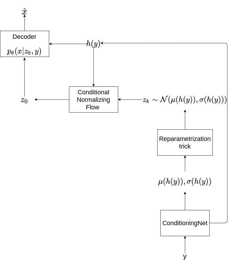
(b) PFVAE inference scheme.

Figure 1: PFVAE’s train and inference schemes.

V Architecture Details

Both the Encoder and Conditioning networks are simple gated convolutional neural networks [34]. They are both composed by $4$ gated blocks, illustrated in Figure 2. At each of these blocks, the temporal dimension is halved by the second gated convolution block.

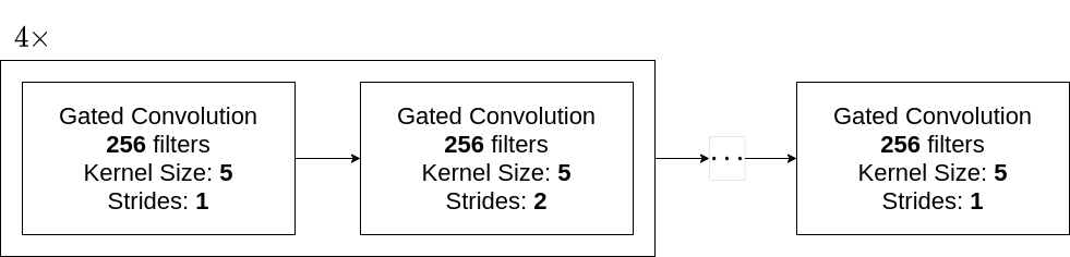
Figure 2: Encoder and Conditioning networks.

Additionally, these two networks only differ in the final layer. After the last Gated Convolution, two convolutional layers in the Conditioning network receive the hidden state $h(y)$, outputting $\mu(h(y))$ and $\sigma(h(y))$. These convolutional layers have $10$ filters of size $1$ and stride $1$. The encoder network has one additional convolutional layer with $10$ filters of size $1$ and stride $1$.

Therefore, the Encoder receives the concatenated vectors $[x;y]$ and outputs the latent representation $z_{0}$, whereas the Conditioning network receives $y$, encodes it into a rich representation $h(y)$ and into the base distribution parameters $\mu(h(y))$ and $\sigma(h(y))$.

The Decoder network is a straightforward neural network responsible for decoding $z_{0}$ back to the $x$ space.

Thus, the Decoder Network is composed of $4$ decoder blocks followed by two simple convolutional layers.

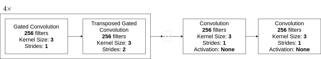
Figure 3: Decoder network.

The CNF network is responsible for learning the prior distribution $\pi(z_{0}|y)$. This network consists of $8$ stacked step-flow blocks [13], which, in it turns, is a stacking of an Actnorm layer, an Invertible $1\times 1$ Convolution layer, and an ACL.

The ACL operators are calculated by a backbone network, which is illustrated in Figure 4.

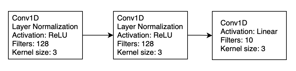
Figure 4: Coupling Layer’s backbone

VI Experiments

Our experiments were conducted on a publicly available dataset [14] that contains industrial heavy-machinery data collected at a Brazilian poultry feed factory. The dataset provides measurements individually collected from eight machines and the factory’s main voltage distribution board (the aggregated data). The available data consists of time series, sampled at 1 Hz, of the following electrical quantities: the RMS voltage, the RMS current, the active power, the reactive power, the apparent power, and the active energy.

The appliance measurements are processed to create an overlapping grid of intervals used as inputs and ground-truth targets by our model. The windows width was decided during our preliminary experiments. We found that intervals of size 256 are long enough to capture most machinery activations. Increasing or decreasing the window size could improve some individual machinery results. Still, since our goal is to work with a single model, intervals of size 256 presented promising results.

The resulting dataset comprises 19.074 appliance samples. Figure 5 presents an aggregated appliance interval and its respective per-machinery active power demand (the targets) taken from the resulting dataset. The data is normalized per-channel by the mean and standard deviation.

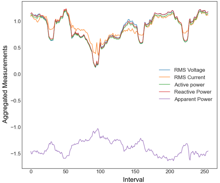
(a) Aggregate measurements’ features.

(b) Appliance-by-appliance power demand.

Figure 5: Example of a window of data present in the dataset.

In all experiments, the model performance is evaluated using two commonly used metrics in NILM tasks [35]: the normalized disaggregation error (NDE) and the signal aggregated error (SAE). Those metrics are calculated from the average of $20$ samples taken with the trained models using the aggregated data $y$ as input.

All models are trained via gradient descent with mini-batches of size $50$ to maximize the equation 3. Thus, the PFVAE is trained on a Google Cloud TPU v2-8 node for $2,000$ epochs using Adam optimizer [36] with its default parameters and a learning rate of $0.00007$.

Cross-Validation

This experiment is performed in a 7-fold cross-validation (CV) setting [37]. The training procedure takes on average 17 hours per cross-validation iteration. Additionally, we perform the CV apart for the milling machines (MI and MII) because the available data is smaller for them. Table I compares the obtained metrics with the WaveNet (WN) model , proposed by the previous work [2] on the same dataset.

TABLE I: Performance comparison between the PFVAE and the Wavenet (WN) models.

	NDE
	WN	PFVAE
PI	0.045 $\pm$ 0.002	0.032 $\pm$ 0.005
PII	0.056 $\pm$ 0.002	0.027 $\pm$ 0.005
DPCI	0.08 $\pm$ 0.01	0.031 $\pm$ 0.004
DPCII	0.202 $\pm$ 0.006	0.034 $\pm$ 0.004
EFI	0.046 $\pm$ 0.0004	0.125 $\pm$ 0.031
EFII	0.041 $\pm$ 0.003	0.042 $\pm$ 0.007
MI	0.08 $\pm$ 0.02	0.015 $\pm$ 0.002
MII	0.06 $\pm$ 0.01	0.039 $\pm$ 0.010
	SAE
	WN	PFVAE
PI	0.047 $\pm$ 0.009	0.018 $\pm$ 0.002
PII	0.022 $\pm$ 0.009	0.016 $\pm$ 0.002
DPCI	0.13 $\pm$ 0.04	0.026 $\pm$ 0.003
DPCII	0.19 $\pm$ 0.02	0.026 $\pm$ 0.003
EFI	0.007 $\pm$ 0.006	0.033 $\pm$ 0.004
EFII	0.016 $\pm$ 0.009	0.020 $\pm$ 0.002
MI	0.09 $\pm$ 0.04	0.063 $\pm$ 0.010
MII	0.03 $\pm$ 0.02	0.073 $\pm$ 0.009

Table 1 shows that the PFVAE consistently improves the metrics in six of the eight machines belonging to the dataset. Analyzing the NDE metric, the improvements go from $28\%$, for the PI machinery, up to $81\%$, for the MI machinery. Additionally, there is an error increase for the EFI and EFII machinery. In turn, improvements in SAE go from $27\%$ for the PII machinery up to $86\%$ for the DPCII machinery. We also observe an error increase for the EFI, EFII, and MII machinery.

The appliance activations are generally related to each other due to the factory’s operation routine, and therefore, learning to represent multiple appliance activations using a single model can be beneficial. Our experiments reinforce this hypothesis, which together with the PFVAE’s higher representational capacity might explain the model’s overall improvements.

Ablation Studies

In the PFVAE architecture, we included two components that work for conditioning the generative process on the aggregate data $y$, which are the $h(y)$ connections in the ACL and the conditioning from the CNF base distribution. We conducted two experiments to investigate the contribution of these components.

In both experiments, the data and the model hyper-parameters were kept constant. The models were trained for six of the eight machines, using $80\%$ of the dataset. The remaining $20\%$ of the dataset was used for testing. We present the total sum and the averaged metrics over the six machines .

First, we compared the complete PFVAE model’s performance against two modified versions. In the first version, we removed the $h(y)$ connections from the ACLs by exchanging them for its simple (and original) version. In the second version, we removed the $\mu(h(y))$ and $\sigma(h(y))$ calculations from the model, fixing the CNF base distribution such that $\pi(z_{k}|y)\sim\mathcal{N}(0,1)$.

TABLE II: Comparison of the averaged and total performance between ablation models.

Total
Ablation	SAE	NDE
Complete Model	0.185	0.373
Simple Affine Layer	0.200	0.452
Standard Normal	2.470	5.301
Averaged
Ablation	SAE	NDE
Complete Model	0.030	0.062
Simple Affine Layer	0.033	0.075
Standard Normal	0.411	0.883

Table II compares the averaged and total resulting metrics of the complete model, the simple ACL, and the standard normal base distribution versions. The standard normal base distribution version results were around ten times worse in both metrics than the other versions.In it turns, the simple ACL version presents very close values for the SAE metric compared against the complete model. However, the significant difference in the NDE indicates that the complete model has a stronger capability to predict appliance instantaneous power demand. Therefore, the usage of the $h(y)$ connections in the ACLs seem to be necessary for the model’s performance.

Next, we analyse the PFVAE model’s performance when varying the number of step-flow blocks used in the CNF. Table III compares the averaged and total resulting metrics for five trained model variants with $2$, $4$, $8$, $16$, and $32$ step-flow blocks.

TABLE III: Comparison of the averaged and total performance between PFVAE variants with 2, 4, 8, 16, and 32 step-flow blocks in the CNF component.

Total
Step-Flows	SAE	NDE
2	1.189	2.317
4	0.261	0.611
8	0.185	0.373
16	0.431	0.663
32	1.598	4.196
Averaged
Step-Flows	SAE	NDE
2	0.198	0.386
4	0.043	0.101
8	0.030	0.062
16	0.071	0.110
32	0.266	0.699

The model with $8$ step-flow blocks presented the best performance in both metrics. It is worth noting that the performance improves by adding more blocks until $8$, starting to degrade when adding more blocks.Thus, the model’s performance degrades with a too shallow and a very deep CNF.

In summary, these experiments suggest that the best version of the PFVAE for the task is the complete model with $8$ step-flow blocks.

VII Conclusions

This work proposes a CDE model to estimate the individual appliances’ power demand from their aggregate power demand measurements. The proposed model joins a CVAE with a CNF model.

We conducted experiments using a publicly available dataset [14] with data collected from a Brazilian poultry feed factory. We observed improvements ranging from $28\%$ up to $81\%$ in NDE and $27\%$ up to $86\%$ in SAE for six dataset machines.

Future work include testing our model using datasets with different appliances and scenarios, such as commercial and residential buildings datasets like [17][38]. Additionally, natural gas and water usage may also be monitored by similar methods [8].

Finally, our experimental results show that the proposed model improves the disaggregation performance for most appliances belonging to the dataset.

Appendix A Ablation Studies Details

Conditioning Ablations

Section VI of the paper presents ablation studies in the PFVAE’s components responsible for conditioning the generative process in the aggregate data $y$. Three models were trained in the experiment:

1. Simple Affine Layer - We removed the conditioning $h(y)$ connections from the affine coupling layers by exchanging them for their original version. Figure 6 illustrates the Simple Affine Layer ablation training and inference schemes.

   

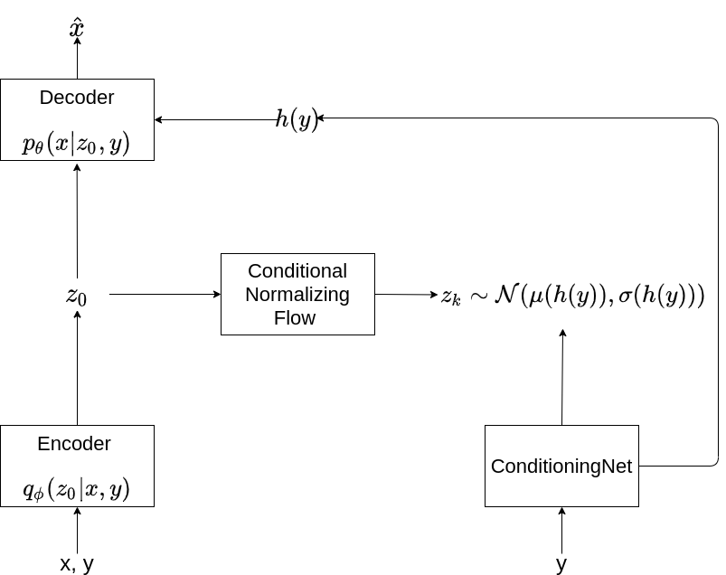
   (a) Training scheme.

   

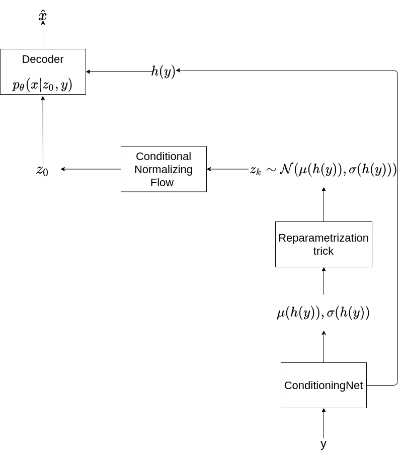
   (b) Inference scheme.

   Figure 6: Simple Affine Layer ablation train and inference schemes.

2. Standard Normal - We removed the conditioning from the $z_{k}$ base distribution, in the CNF, by fixing its parameters to match the diagonal Standard Normal such that $\pi(z_{k}|y)\sim\mathcal{N}(0,I)$. Consequently, we removed the $\mu(h(y))$ and $\sigma(h(y))$ calculations from the model. Figure 7 illustrates the Standard Normal ablation training and inference schemes.

   

   (a) Training scheme.

   

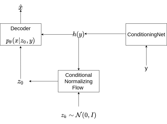
   (b) Inference scheme.

   Figure 7: Standard Normal ablation train and inference schemes.

3. Full PFVAE Model - This variant is the complete PFVAE model with no modifications. Figure 8 illustrates the Full PFVAE Model ablation training and inference schemes. Note, this figure is the same one presented in the paper’s section IV, and we are showing it here again for easier comparison.

   

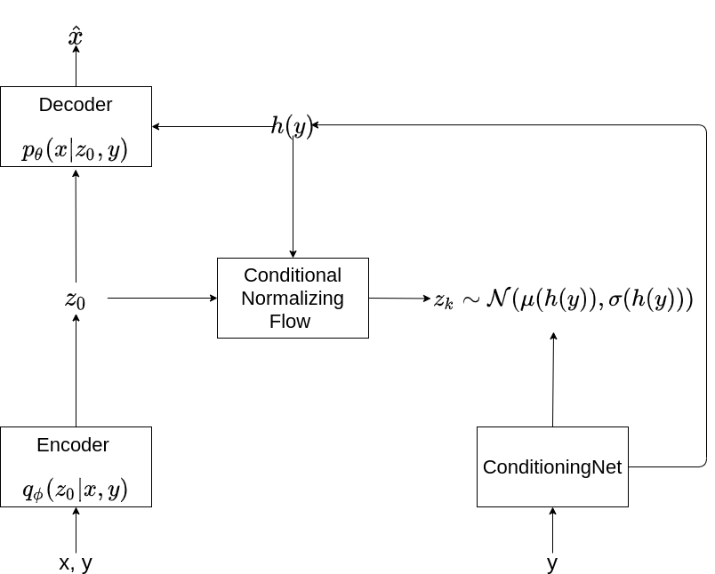
   (a) Training scheme.

   

   (b) Inference scheme.

   Figure 8: Full PFVAE model train and inference schemes.

Table IV compares the models’ performance per machine.

TABLE IV: Per-machine performance comparison between PFVAE’s ablation variants.

	Simple Affine		Standard Normal		Full Model
	SAE	NDE	SAE	NDE	SAE	NDE
PI	0.034	0.083	0.149	0.242	0.018	0.042
PII	0.036	0.071	0.154	0.224	0.020	0.044
DPCI	0.030	0.046	0.535	0.695	0.035	0.052
DPCII	0.029	0.048	0.542	0.701	0.036	0.055
EFI	0.046	0.153	0.759	2.863	0.047	0.131
EFII	0.022	0.047	0.329	0.574	0.027	0.046
TOTAL	0.200	0.452	2.470	5.301	0.185	0.373

Additionally, figure 9 compares the loss learning curve of each ablation model. The full model presents a more stable curve and higher end-loss, indicating a more regularized model with less over-fitting.

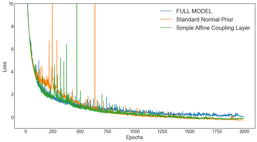
Figure 9: Conditioning Ablations Learning Curves Comparison.

Step-Flows

Section VI of the paper presents ablation studies in the number of step-flow blocks used in the PFVAE’s CNF component. Five models were trained in the experiment, each with $2$, $4$, $8$, $16$, and $32$ step-flow blocks in the CNF component.

Table V compares the achieved NDE, per machine, by the five trained models.

TABLE V: NDE comparison between PFVAE variants with 2, 4, 8, 16, and 32 step-flow blocks in the CNF component.

	NDE
	2	4	8	16	32
PI	0.070	0.094	0.042	0.051	0.039
PII	0.085	0.064	0.044	0.046	0.046
DPCI	0.337	0.073	0.052	0.107	0.513
DPCII	0.412	0.076	0.055	0.118	0.529
EFI	1.192	0.220	0.131	0.272	2.838
EFII	0.218	0.083	0.046	0.066	0.228
TOTAL	2.317	0.611	0.373	0.663	4.196

Table VI compares the achieved SAE, per machine, by the five trained models.

TABLE VI: SAE comparison between PFVAE variants with 2, 4, 8, 16, and 32 step-flow blocks in the CNF component.

	SAE
	2	4	8	16	32
PI	0.036	0.037	0.018	0.035	0.036
PII	0.043	0.031	0.020	0.033	0.036
DPCI	0.280	0.043	0.035	0.088	0.355
DPCII	0.272	0.045	0.035	0.093	0.344
EFI	0.388	0.062	0.047	0.118	0.631
EFII	0.168	0.040	0.027	0.062	0.194
TOTAL	1.189	0.261	0.185	0.431	1.598

Additionally, figure 10 compares the loss learning curve of each ablation model. The models with 8 and 16 step-flow blocks have more stable learning curves than the others. However, the model with 4 step-flow blocks has the lowest end-loss, which is very close to the 8 blocks model’s end-loss. We believe that it indicates that the number of step-flow blocks influences in both the CNF representational capability and in the model regularization. Thus, the greater the number of step-flow blocks, the greater the CNF representational capability becomes, and the more regularized the model. This could explain the reason why model with 16 step-flow blocks presented an end-loss greater than the model with 4 step-flow blocks, despite having a more stable learning curve.

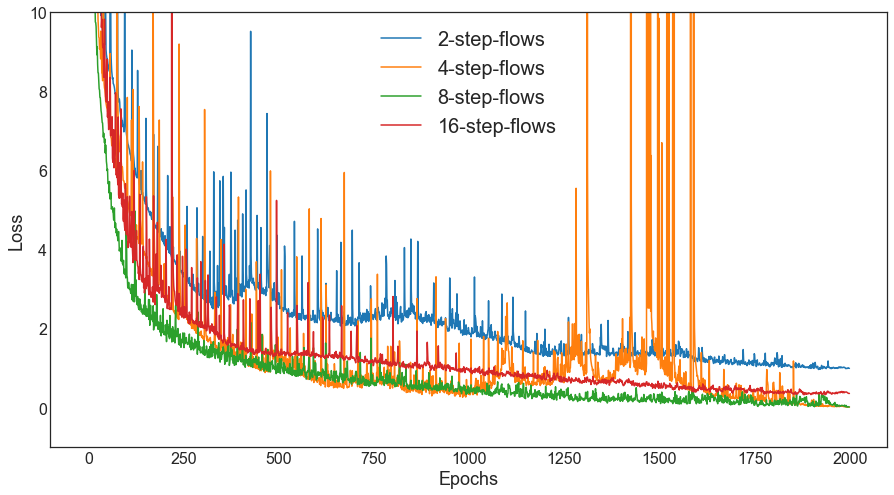
Figure 10: Step-Flows Ablations Learning Curves Comparison.

Appendix B Visual Comparison Plots for Qualitative Analysis

This section presents plots for the visual comparison between the model estimate and the actual active power, the ground truth, for six of the eight devices in the data set. Here all presented estimations are taken from the full PFVAE, with 8 step-flows blocks and trained with $80\%$ of the dataset. Comparisons are made in the dataset test set. Moreover, all plots present the actual active power (ground truth), the mean of 10 samples taken from the model, and the estimated confidence interval computed at the $95\%$ confidence level.

Palletizer I - PI

Figure 11 presents 25 PFVAE estimates compared to the PI machine’s ground thruth.

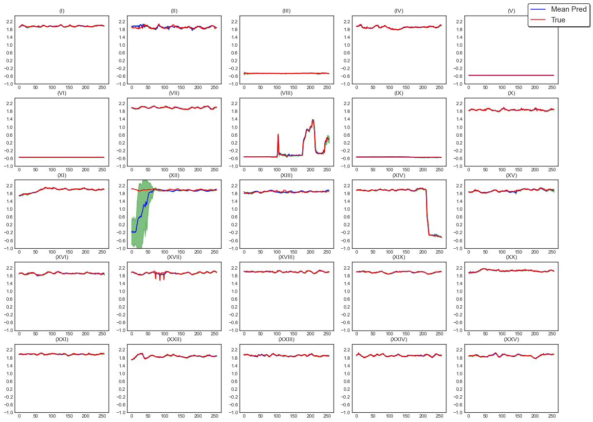
Figure 11: Visual comparison between the model estimates and the Palletizer machine I (PI) ground truth.

Additionally, figure 12 presents re-scaled plots for 3 of the 25 comparisons to observe the signal in a more detailed view and illustrate the inferred confidence interval (the green shaded area).

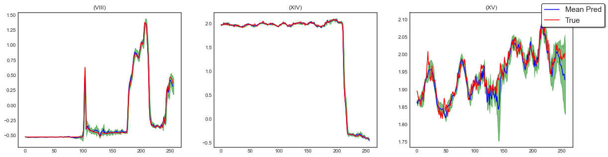
Figure 12: PI re-scaled plots.

Palletizer II - PII

Figure 14 presents 25 PFVAE estimates compared to the PII machine’s ground truth.

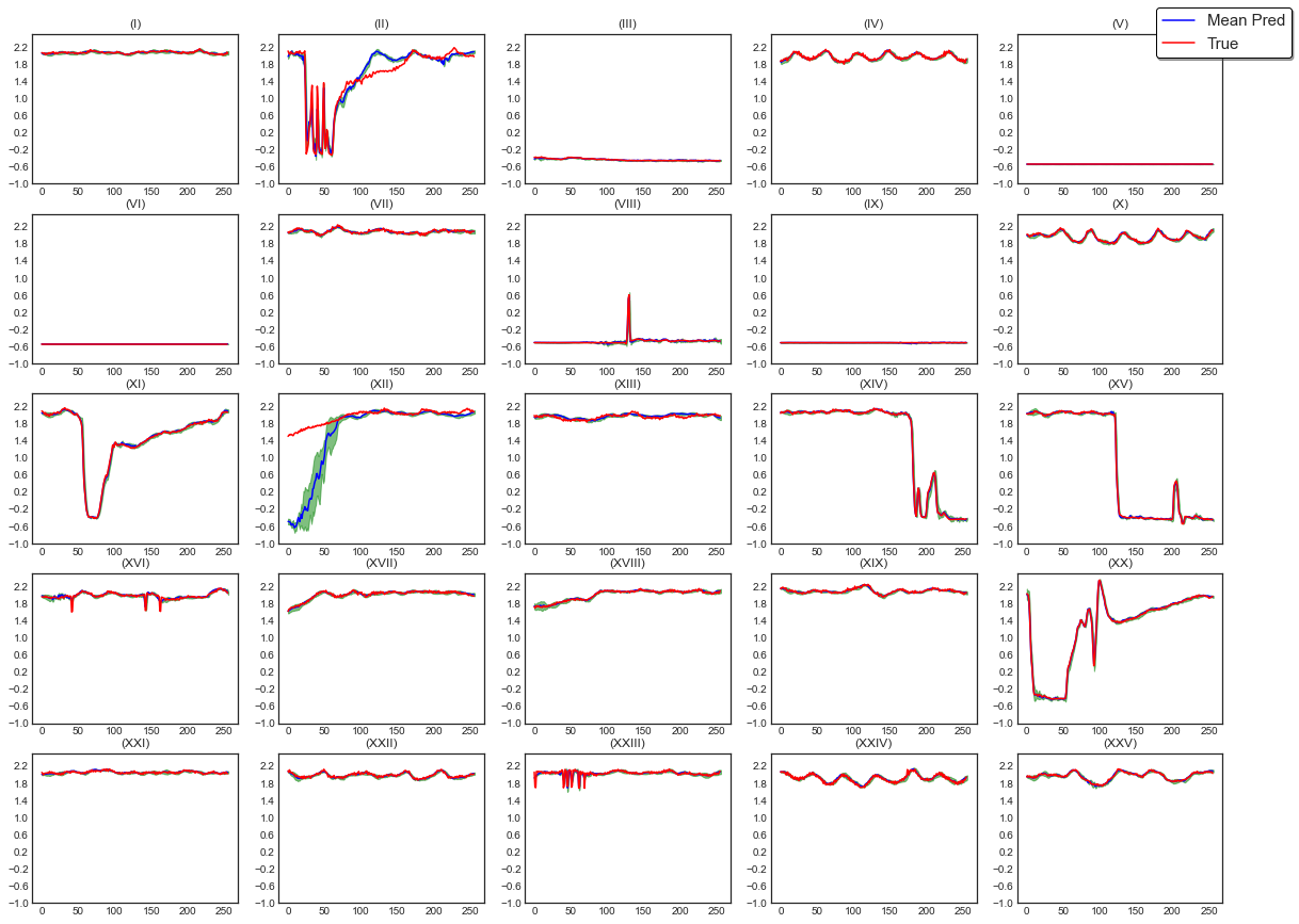
Figure 13: Visual comparison between the model estimates and the Palletizer machine II (PII) ground truth.

Additionally, figure 14 presents re-scaled plots for 3 of the 25 comparisons to observe the signal in a more detailed view and illustrate the inferred confidence interval (the green shaded area).

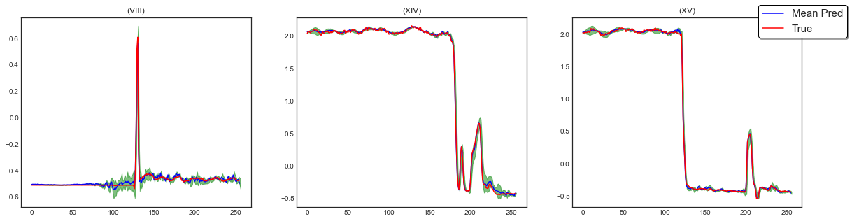
Figure 14: PII re-scaled plots.

Pouble-Pole Contactor I - DPCI

Figure 15 presents 25 PFVAE estimates compared to the DPCI machine’s ground truth.

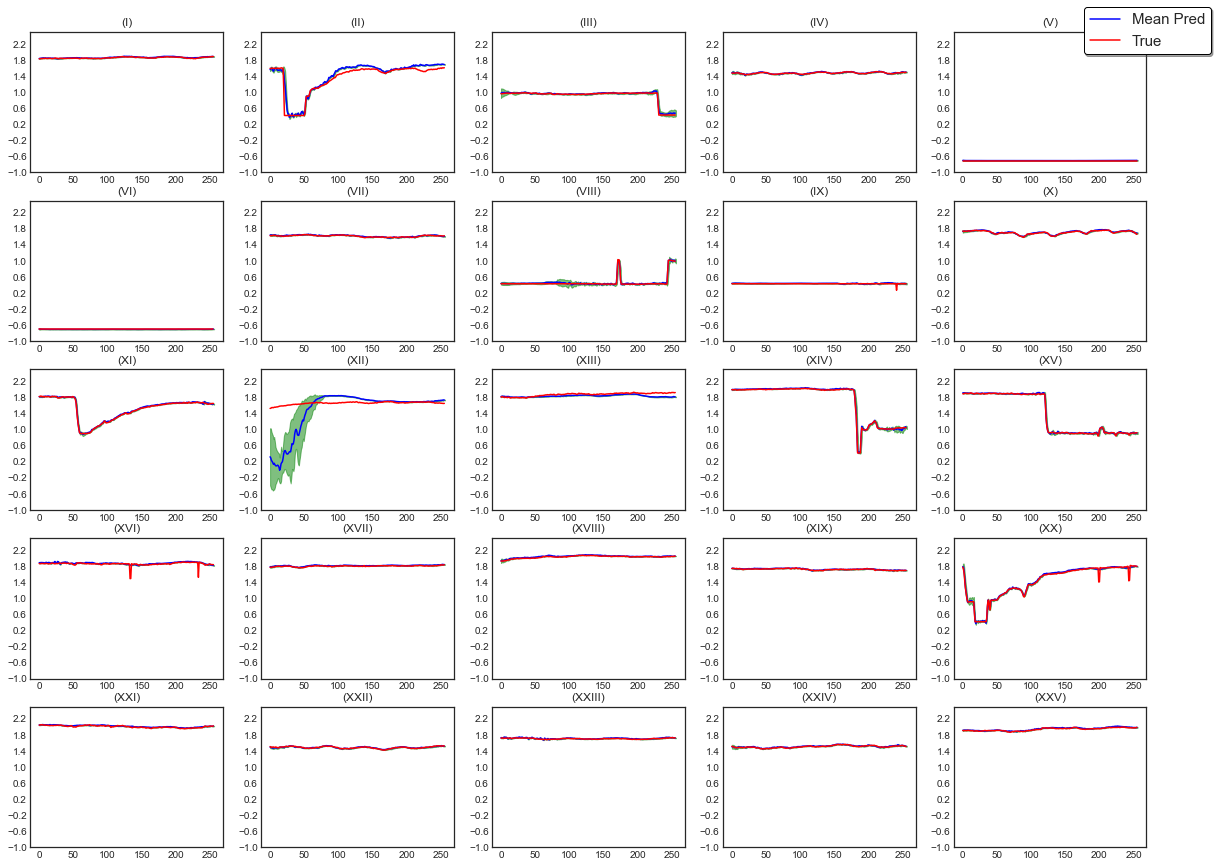
Figure 15: Visual comparison between the model estimates and the ground truth for the Double-Pole Contactor machine I (DPCI).

Additionally, figure 16 presents re-scaled plots for 3 of the 25 comparisons to observe the signal in a more detailed view and illustrate the inferred confidence interval (the green shaded area).

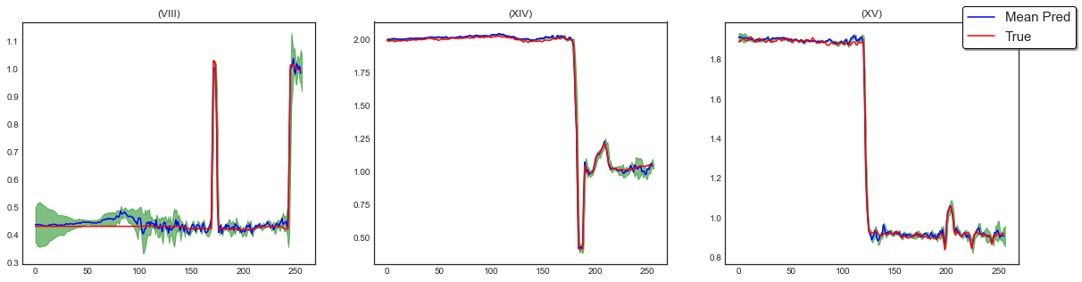
Figure 16: DPCI re-scaled plots.

Double-Pole Contactorr II - DPCII

Figure 17 presents 25 PFVAE estimates compared to the DPCII machine’s ground truth.

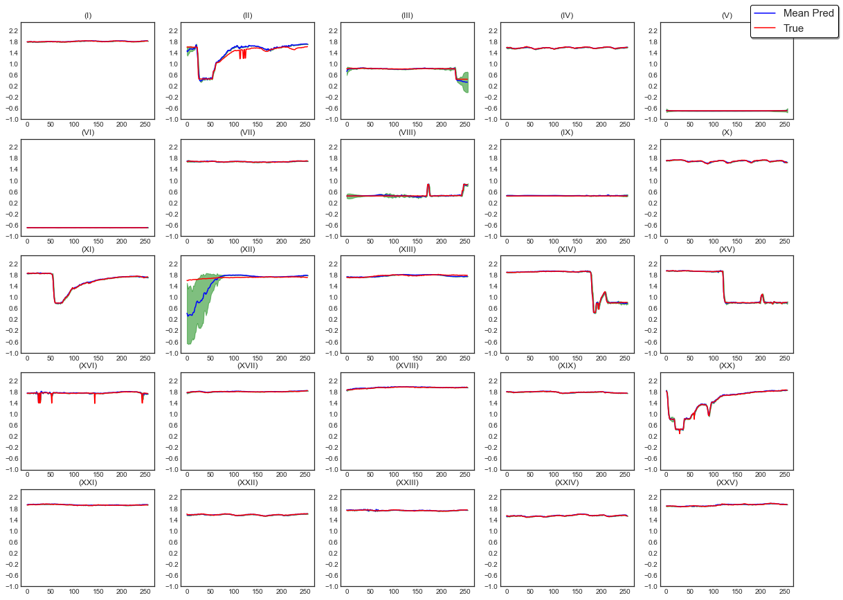
Figure 17: Visual comparison between the model estimates and the Double-Pole Contactor machine II (DPCII) ground truth.

Additionally, figure 18 presents re-scaled plots for 3 of the 25 comparisons to observe the signal in a more detailed view and illustrate the inferred confidence interval (the green shaded area).

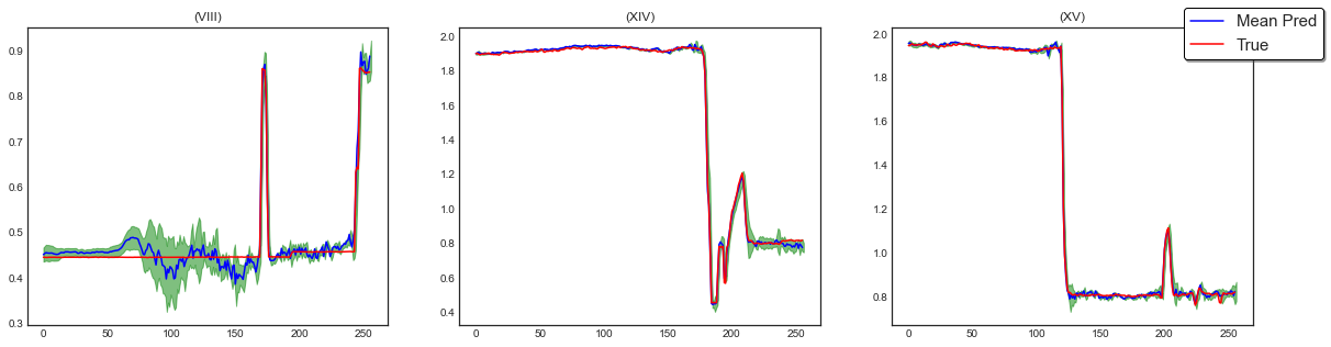
Figure 18: DPCII re-scaled plots.

Exhaust Fan I - EFI

Figure 19 presents 25 PFVAE estimates compared to the EFI machine’s ground truth.

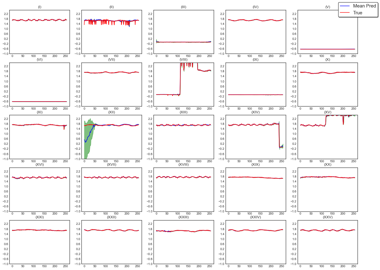
Figure 19: Visual comparison between the model estimates and the Exhaust Fan machine I (EFI) ground truth.

Additionally, figure 20 presents re-scaled plots for 3 of the 25 comparisons to observe the signal in a more detailed view and illustrate the inferred confidence interval (the green shaded area).

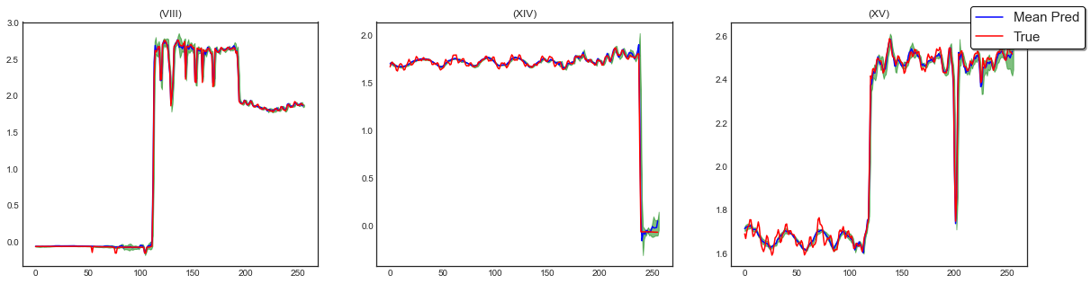
Figure 20: EFI re-scaled plots.

Exhaust Fan II - EFII

Figure 21 presents 25 PFVAE estimates compared to the EFII machine’s ground truth.

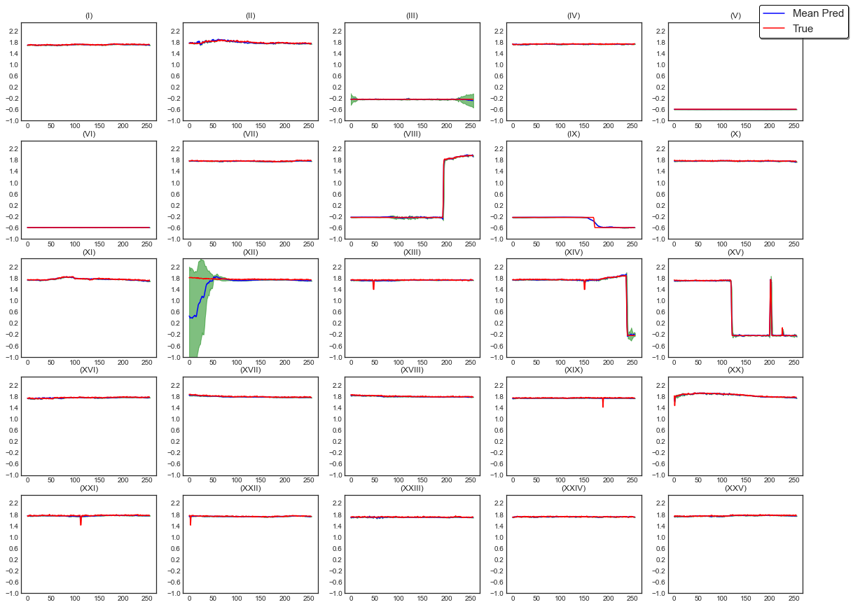
Figure 21: Visual comparison between the model estimates and the ground truth for the Exhaust Fan machine II (EFII).

Additionally, figure 22 presents re-scaled plots for 3 of the 25 comparisons to observe the signal in a more detailed view and illustrate the inferred confidence interval (the green shaded area).

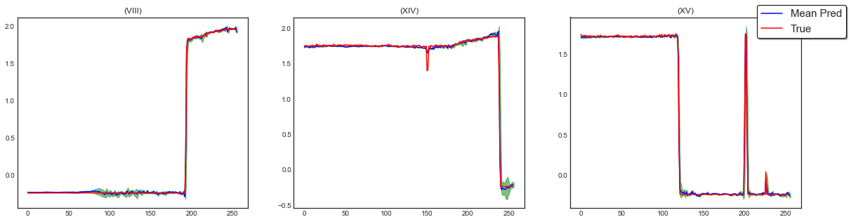
Figure 22: EFII re-scaled plots.

References

- [1] J. Kelly and W. J. Knottenbelt, “Neural nilm: Deep neural networks applied to energy disaggregation,” ArXiv, vol. abs/1507.06594, 2015.
- [2] P. B. M. Martins, J. G. R. C. Gomes, V. B. Nascimento, and A. R. de Freitas, “Application of a deep learning generative model to load disaggregation for industrial machinery power consumption monitoring,” 2018 IEEE International Conference on Communications, Control, and Computing Technologies for Smart Grids, pp. 1–6, 2018.
- [3] J. G. Roos, I. E. Lane, E. C. Botha, and G. P. Hancke, “Using neural networks for non-intrusive monitoring of industrial electrical loads,” Conference Proceedings. 10th Anniversary. IMTC/94. Advanced Technologies in I & M. 1994 IEEE Instrumentation and Measurement Technolgy Conference (Cat. No.94CH3424-9), pp. 1115–1118 vol.3, 1994.
- [4] H. Yang, H. Chang, and C. Lin, “Design a neural network for features selection in non-intrusive monitoring of industrial electrical loads,” in 2007 11th International Conference on Computer Supported Cooperative Work in Design, 2007, pp. 1022–1027.
- [5] Y. Lin and M. Tsai, “A novel feature extraction method for the development of nonintrusive load monitoring system based on bp-ann,” in 2010 International Symposium on Computer, Communication, Control and Automation (3CA), vol. 2, 2010, pp. 215–218.
- [6] A. G. Ruzzelli, C. Nicolas, A. Schoofs, and G. M. P. O’Hare, “Real-time recognition and profiling of appliances through a single electricity sensor,” in 2010 7th Annual IEEE Communications Society Conference on Sensor, Mesh and Ad Hoc Communications and Networks, 2010, pp. 1–9.
- [7] H. Chang, P. Chien, L. Lin, and N. Chen, “Feature extraction of non-intrusive load-monitoring system using genetic algorithm in smart meters,” in 2011 IEEE 8th International Conference on e-Business Engineering, 2011, pp. 299–304.
- [8] G. Hart, “Nonintrusive appliance load monitoring,” Proceedings of the IEEE, vol. 80, no. 12, pp. 1870–1891, 1992.
- [9] D. P. Kingma and M. Welling, “Auto-encoding variational bayes,” CoRR, vol. abs/1312.6114, 2013.
- [10] K. Sohn, H. Lee, and X. Yan, “Learning structured output representation using deep conditional generative models,” in NIPS, 2015.
- [11] L. Dinh, D. Krueger, and Y. Bengio, “Nice: Non-linear independent components estimation,” CoRR, vol. abs/1410.8516, 2014.
- [12] L. Dinh, J. Sohl-Dickstein, and S. Bengio, “Density estimation using real nvp,” ArXiv, vol. abs/1605.08803, 2016.
- [13] D. P. Kingma and P. Dhariwal, “Glow: Generative flow with invertible 1x1 convolutions,” in NeurIPS, 2018.
- [14] P. B. de Mello Martins; Vagner Barbosa Nascimento; Antônio Renato de Freitas; Pedro Bittencourt e Silva; Raphael Guimarães Duarte Pinto, “Industrial machines dataset for electrical load disaggregation,” 2018. [Online]. Available: http://dx.doi.org/10.21227/cg5v-dk02
- [15] M. Zeifman and K. Roth, “Nonintrusive appliance load monitoring: Review and outlook,” IEEE Transactions on Consumer Electronics, vol. 57, 2011.
- [16] K. C. Armel, A. Gupta, G. Shrimali, and A. Albert, “Is disaggregation the holy grail of energy efficiency? the case of electricity,” Energy Policy, vol. 52, pp. 213–234, 2013.
- [17] J. Kelly and W. Knottenbelt, “The UK-DALE dataset, domestic appliance-level electricity demand and whole-house demand from five UK homes,” Scientific Data, vol. 2, no. 150007, 2015.
- [18] R. Bonfigli, A. Felicetti, E. Principi, M. Fagiani, S. Squartini, and F. Piazza, “Denoising autoencoders for non-intrusive load monitoring: Improvements and comparative evaluation,” Energy and Buildings, vol. 158, pp. 1461–1474, 2018.
- [19] J. Z. Kolter and T. Jaakkola, “Approximate inference in additive factorial hmms with application to energy disaggregation,” in AISTATS, 2012.
- [20] C. Zhang, M. Zhong, Z. Wang, N. Goddard, and C. Sutton, “Sequence-to-point learning with neural networks for nonintrusive load monitoring,” in AAAI, 2018.
- [21] Z. Ghahramani and M. I. Jordan, “Factorial hidden markov models,” Machine Learning, vol. 29, pp. 245–273, 1997.
- [22] A. van den Oord, S. Dieleman, H. Zen, K. Simonyan, O. Vinyals, A. Graves, N. Kalchbrenner, A. W. Senior, and K. Kavukcuoglu, “Wavenet: A generative model for raw audio,” ArXiv, vol. abs/1609.03499, 2016.
- [23] M. I. Jordan, Z. Ghahramani, T. Jaakkola, and L. Saul, “An introduction to variational methods for graphical models,” Machine Learning, vol. 37, pp. 183–233, 1999.
- [24] J. Walker, C. Doersch, A. Gupta, and M. Hebert, “An uncertain future: Forecasting from static images using variational autoencoders,” in ECCV, 2016.
- [25] C. Doersch, “Tutorial on variational autoencoders,” ArXiv, vol. abs/1606.05908, 2016.
- [26] L. Ardizzone, C. Lüth, J. Kruse, C. Rother, and U. Köthe, “Guided image generation with conditional invertible neural networks,” ArXiv, vol. abs/1907.02392, 2019.
- [27] C. Winkler, D. Worrall, E. Hoogeboom, and M. Welling, “Learning likelihoods with conditional normalizing flows,” ArXiv, vol. abs/1912.00042, 2019.
- [28] R. V. Berg, L. Hasenclever, J. Tomczak, and M. Welling, “Sylvester normalizing flows for variational inference,” in UAI, 2018.
- [29] A. Bhattacharyya, M. Hanselmann, M. Fritz, B. Schiele, and C. Straehle, “Conditional flow variational autoencoders for structured sequence prediction,” ArXiv, vol. abs/1908.09008, 2019.
- [30] Z. M. Ziegler and A. M. Rush, “Latent normalizing flows for discrete sequences,” ArXiv, vol. abs/1901.10548, 2019.
- [31] D. Nielsen, P. Jaini, E. Hoogeboom, O. Winther, and M. Welling, “Survae flows: Surjections to bridge the gap between vaes and flows,” in Advances in Neural Information Processing Systems, H. Larochelle, M. Ranzato, R. Hadsell, M. F. Balcan, and H. Lin, Eds., vol. 33. Curran Associates, Inc., 2020, pp. 12 685–12 696. [Online]. Available: https://proceedings.neurips.cc/paper/2020/file/9578a63fbe545bd82cc5bbe749636af1-Paper.pdf
- [32] G. Yang, X. Huang, Z. Hao, M.-Y. Liu, S. Belongie, and B. Hariharan, “Pointflow: 3d point cloud generation with continuous normalizing flows,” in 2019 IEEE/CVF International Conference on Computer Vision (ICCV), 2019, pp. 4540–4549.
- [33] X. Ma, C. Zhou, X. Li, G. Neubig, and E. Hovy, “FlowSeq: Non-autoregressive conditional sequence generation with generative flow,” in Proceedings of the 2019 Conference on Empirical Methods in Natural Language Processing and the 9th International Joint Conference on Natural Language Processing (EMNLP-IJCNLP). Hong Kong, China: Association for Computational Linguistics, Nov. 2019, pp. 4282–4292. [Online]. Available: https://www.aclweb.org/anthology/D19-1437
- [34] Y. Dauphin, A. Fan, M. Auli, and D. Grangier, “Language modeling with gated convolutional networks,” in ICML, 2017.
- [35] M. Zhong, N. Goddard, and C. Sutton, “Signal aggregate constraints in additive factorial hmms, with application to energy disaggregation,” in Advances in Neural Information Processing Systems, Z. Ghahramani, M. Welling, C. Cortes, N. Lawrence, and K. Q. Weinberger, Eds., vol. 27. Curran Associates, Inc., 2014. [Online]. Available: https://proceedings.neurips.cc/paper/2014/file/2d1b2a5ff364606ff041650887723470-Paper.pdf
- [36] D. P. Kingma and J. Ba, “Adam: A method for stochastic optimization,” CoRR, vol. abs/1412.6980, 2015.
- [37] R. Kohavi, “A study of cross-validation and bootstrap for accuracy estimation and model selection,” in Proceedings of the 14th International Joint Conference on Artificial Intelligence - Volume 2, ser. IJCAI’95. San Francisco, CA, USA: Morgan Kaufmann Publishers Inc., 1995, pp. 1137–1143. [Online]. Available: http://dl.acm.org/citation.cfm?id=1643031.1643047
- [38] J. Z. Kolter and M. J. Johnson, “Redd: A public data set for energy disaggregation research,” in Workshop on data mining applications in sustainability (SIGKDD), San Diego, CA, vol. 25, no. Citeseer, 2011, pp. 59–62.