Ray-tracing a small orbital mission for soft-X-ray polarimetry

Abstract

X-ray polarimetry is still largely uncharted territory. With the upcoming launch of IXPE, we will learn a lot more about X-ray polarization at energies above 2 keV, but so far no current or accepted mission provides observational capabilities below 2 keV. We present ray-tracing results for a small orbital mission that could be launched within NASA’s Pioneer or SmallSat cost-cap to provide X-ray polarimetry below 2 keV. The design is based on the use of laterally-graded multi-layer (ML) mirrors, a concept that we have developed theoretically for the REDSoX Polarimeter[1], for which most components have been verified in the laboratory. In this contribution, we describe a single channel orbital mission based on the same idea, but modified to the unique cost and space requirements. All results scale up easily to two or more polarimetry channels. Scaling up would simply increase the effective area and reduce the need to rotate the instrument to measure the different polarization directions. In particular, we use the ray-traces to define the maximum size of the dispersion gratings and to determine an alignment budget.

1 INTRODUCTION

X-rays can provide unique insight into the hot and energetic universe. While X-ray photometry and spectroscopy is now routinely performed with a number of missions, most prominently XMM-Newton and Chandra, there is no currently operating observatory to perform X-ray polarimetry and only for a single source (the Crab nebula) has there ever been a significant detection of polarized X-rays[2, 3]. IXPE[4] will be launched in 2021 and provide this capability for X-rays above 2 keV, but there is still no instrument in sight for soft X-ray polarimetry. Yet, a range of open science questions for several classes of astrophysical sources can only be answered with soft X-ray polarimetry.

In this paper we present ray-trace studies for a a small orbital mission for soft x-ray polarimetry, which is described in section 2. In section 3 we describe the setup of our ray-trace simulations. From those, we can predict the performance, most importantly effective area and modulation factor (section 4, perform trade-studies on shape and the size of the gratings used in the design (section 5, and evaluate the influence of alignment errors and other non-ideal effects (section 6). We end with a short summary in section 7.

2 MISSION OVERVIEW

Over the years, we have developed and refined a design for a soft X-ray polarimeter, called “REDSoX”, which is based on reflection off a laterally-graded multi-layer (ML) mirror. Details of the REDSoX design are discussed in Ref. 1, more details of ray-trace calculations are presented in Ref. 5. In short, X-rays are focused into a converging beam using a mirror. Beyond the mirror, the photons encounter critical-angle transmission (CAT) gratings[6, 7, 8, 9]. A fraction of the photons passes straight through the gratings onto an imaging detector, which can be used to confirm the accuracy of the pointing and provide an X-ray spectrum with the intrinsic energy resolution of the detector. Most photons, however, are diffracted. By selecting the blaze angle (the angle between the grating normal and the direction of the incoming photons), we can optimize the fraction of photons diffracted into the first order. Photons of longer wavelengths are diffracted farther and thus hit the focal plane farther away from the direct image than photons with shorter wavelengths. A multi-layer mirror is located in the focal plane. The thickness of the layers varies with position (“laterally graded”) and is chosen such that every photon interacts with the mirror at a position where the mirror spacing matches Bragg condition for photons of that wavelength[1, 5]. The mirror is tilted by about 45 degrees with respect to the incoming photons, and thus only photons with one polarization direction are reflected (“Brewster angle”), while photons with a perpendicular polarization are absorbed. A CCD detects the reflected photons. The requirement to match the photon position to the Bragg peak on the multi-layer mirror sets a limit to the width of the mirror point-spread function in the dispersion direction. We achieve this by sub-aperturing, i.e. we use only wedge-shaped mirror modules and not full circles.

Measurements at several angles are required to reconstruct the polarization fraction and angle. In our design, this can be achieved with a single multi-layer mirror if the entire instrument rotates (either continuously or in steps) throughout the observation or with two or three channels, each with its own sub-aperture, multi-layer mirror and detector, that are rotated with respect to each other.

REDSoX is designed as a sounding rocket payload with very short exposure times, but relaxed mass and volume requirements. In this paper, we present ray-traces for a variant of the REDSoX design optimized for a small orbital mission, e.g. in NASA’s Astrophysics Pioneer or SmallSat program. Compared to REDSoX, we need to shorten the focal length to fit the mission into the envelope of a secondary payload, such as when mounted to an ESPA grande ring. While the mirror area may be smaller, we can integrate for days to months in an orbital mission while a sounding rocket gives only a few minutes of observing time.

Most of the trades and studies done for REDSoX[5] are applicable here, too, just with different numbers for the focal length, but others are unique to this design, e.g. the much longer exposure times require a much more careful estimate of the background that is picked up in the detectors. While the sounding rocket REDSoX is designed with three polarization channels, an orbital mission with much longer exposure times can work with just one or two channels because lower effective areas can be compensated by longer exposure times.

In this work, we consider a system with a focal length of just 1.25 m and a single polarimetry channel. An overview of the design is shown in Figure 1. This matches our submitted Astrophysics Pioneer proposal (dubbed “PiSoX” for Pioneer Soft X-ray polarimeter) and represents the simplest possible instrument to measure soft X-ray polarization. It is easy to extend this design by adding another polarimetry channel for redundancy, increased effective area, and the opportunity to measure fast changes in the polarization (since two polarization directions are observed simultaneously, instead of rotating the instrument), but for simplicity we will call the instrument “PiSoX” for the remainder of this article.

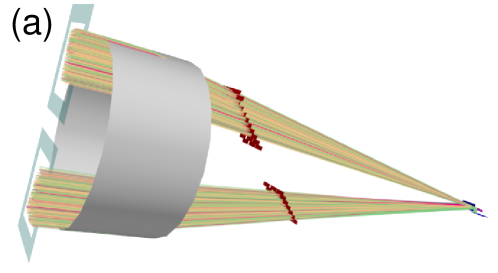
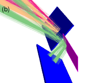
Figure 1: 3D rendering of the instrument design and a ray-trace for monoenergetic rays of 0.3 keV. The ray-trace setup makes some simplifications. In particular, the mirror is not modeled in 3D, but approximated by a 2D lens. The position of the mirror modules is indicated by a cylinder that has the same radius as the outermost mirror surface. This is a monochromatic simulation with photon energies of 0.3 keV. Rays are colored according to the grating diffraction order. The zeroth order is shown with orange rays, the first order with green rays. The green rays bounce of the multilayer-mirror (purple) before they hit a detector (blue). The second detector (also blue) images the zeroth order, but also photons diffracted into order -1 (red rays). panel a: View of the full instrument. The astrophysical source is located towards the left. Rays are shown starting at the entrance aperture. panel b: Zoom into the focal plane with multi-layer mirror (purple) and two detectors (blue).

Figure 1 shows a ray-trace through our one-channel system. All rays in the figure have the same energy (0.3 keV). Because the mirrors deliver a converging beam, rays have different angles with respect to the ML mirror. Because of that, they require a slightly different period of the layers of the ML mirror to match the Bragg peak, and consequently, they have to be diffracted to a different position on the ML mirror. This is the origin of the stair-stepped arrangement of the CAT gratings[1, 5]. In panel (b) of the figure, it can be seen that the rays fall into two groups depending on if they pass through the upper or lower sector of gratings.

3 SETUP FOR RAY-TRACES

We perform a geometric ray-trace with the MARXS code, which follows individual rays through the system from the entrance aperture to the detector. Simulations are performed with MARXS 1.2[10, 11]. MARXS is written in Python and available under the GNU license v3. The code is available on github. Specific code for the simulations of the instrument shown here is also available; we used the version with commit hash 13b10be. More details on the code can be found in proceedings describing its application for other missions[12, 13].

Every simulation contains some simplification of reality, e.g., because certain aspects of the design are not known yet, laboratory data about performance must be extrapolated, or simply because computational cost puts limits on how many photons can be run through a simulation. Our simulations are set up with a relatively simplistic mirror model. Instead of a three dimensional structure, the mirror is implemented as plane perpendicular to the optical axis. When rays intersect the plane, their directions are modified as if they pass a perfect lens. In the next step, additional scatter in the plane of reflection is added. For each ray, the scattering angle is drawn from a Gaussian distribution, where the width of the distribution is tuned to achieve a PSF size that matches the PSFs measured or expected for the type of mirror used. We use 12 arcsec for the $\sigma$ of the Gaussian.

Our instrument uses CAT gratings manufactured from Si wafers at the MIT Space Nanotechnology Laboratory [6, 7, 8, 9]. The grating efficiency of these gratings is calculated based on simulations and verified in the laboratory; a table of efficiencies is an input to our simulations. The high aspect-ratio grating bars are 4 $\mu$m deep and supported by an L1 support structure running perpendicular to the grating bars themselves and the entire membrane (bars and L1) is mechanically stabilized by a hexagonal L2 support structure, which is 0.5 mm deep. Absorption and diffraction of photons by the L1 and L2 support structures is included in our simulations. The grating membrane is surrounded by a 1.5 mm wide frame of solid Si which is glued into a grating holder. We discuss in section 5.1 that we require the $30\times 10$ mm sized gratings to be bend along the long axis. Laboratory measurement show that bending does not decrease performance[14] and grating alignment has also been proto-typed[15, 16].

Laterally graded multi-layer (ML) mirrors can be made from a variety of materials. We use a Cr/Sc mirror, because this combination of material promises a good reflectivity in the bandpass of interest; ML mirror reflectivities have been verified in the laboratory[17]. The detectors will be CCD ID-94 detectors produced by Lincoln Labs, we use the quantum efficiencies measured for Suzaku CCDs[18] for our ray-traces.

4 PERFORMANCE

The main characteristics of a polarimeter are its effective area and the modulation factor.

4.1 Effective area and modulation factor

In order to determine the modulation factor, we perform simulations for a source that is 100% polarized. Then, we rotate the pointing of the instrument on the sky in small steps so that we can build up the modulation curve. From this curve, the total modulation of the signal can be calculated as $\frac{T-B}{T+B}$, where $T$ is the maximum of the curve and $B$ is the minimum. The energy dependence for effective area and modulation are shown in figure 2.

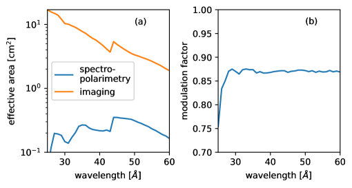
Figure 2: panel a: Effective area. CCD 1 detects the polarized signal, CCD 0 the zeroth order. Because CCD 1 observes rays reflected off the ML mirror, the effective area is much lower than in the CCD 0. panel b:: modulation factor.

4.2 How does an observation look?

Since PiSoX has only a single polarimetry channel, we have to rotate the instrument on the sky to cover enough range in rotation angles to sample all possible polarization directions. We show simulations with the spectrum and flux of Mk 421 assuming the source is fully polarized. In reality, the polarization fraction is going to be $<1$ and might depend on energy. Of course, we can simulate those scenarios, too, but the point here is to show how the data works in principle, so we pick the easiest scenario.

We simulate two observations with different polarization angles on the sky, which are chosen such that the first angle gives the maximal signal and the second one the minimal signal on the polarization channel. In a real observation, that angle is not known a priori and the instrument needs to be rotated continuously or observe at at least three angles to be able to uniquely derive the polarization fraction and angle from the polarization channels alone. Using the zeroth order data as well, then observations at two angles are sufficient.

4.3 Background

For faint sources, background limits the signal-to-noise ratio that can be achieved with very long observations. There are two main components to the background: Particle background and astrophysical sources. We assume that the particle background is independent of the orientation of the spacecraft. With CCD detectors, the main mechanism for reducing background is to select data using the shapes and energies of the detected events. For a dispersive spectro-polarimeter like PiSoX only background events that match the energy of the photons expected at that position on the detector are relevant, reducing the influence of the particle background. Astrophysical background stems from the Cosmic X-ray Background, composed of a soft, thermal Galactic foreground component and power-law component to account for unresolved AGN. The spectral shape and flux of the astrophysical background are taken from an analysis of Abell 1795[19]. We simulate this as a disk of 1 degree radius (limited by the field-of-view of the thermal pre-collimators) to determine how diffuse sky background influences the count rate in the polarization channel. Since dispersed source count rates can be very low, background can potentially become important. On the other hand, the multi-layer mirror will only reflect photons coming with a very specific combination of angle and energy, reducing the background significantly.

For a 100 ks observation, we predict 0.2 cts in the polarimetry channel when extracting the chip area that contains the signal of an on-axis point source. This is an upper limit, because it does not yet consider energy filtering using the intrinsic CCD resolution, which may reduce the background rate by another factor of two or so. The simulation predicts of order 100 counts that spatially overlap with the zeroth order of an on-axis point source, where the exact number scales with the size of the extraction region. The difference in flux between imaging and polarimetry channel is $10^{4}$, while the effective area differs only by one order of magnitude. From this, we can conclude that the ML mirror suppresses the background by about a factor of $10^{3}$. At a flux of $2\frac{\mathrm{ct}}{\mathrm{Ms}}$, we can safely assume that diffuse X-ray emissions is negligible, as several thousand counts are needed to detect polarizations below 10%.

5 TRADES

5.1 Bending gratings

Figure 3: In a converging beam (black rays) the angle between the grating normal and the rays changes with grating position for a flat grating (blue). Bending the grating can compensate for this problem (orange) for gratings that are small compared to the radius. This is true for gratings where the ray through the grating center is normal to the grating (left) and for gratings with a design blaze angle (right).

The grating efficiency of CAT gratings changes with the blaze angle. If the blaze angle is small, i.e. the rays hit the grating parallel to the surface normal, then many rays will end up in the zeroth order. Higher blaze angles favour higher orders. PiSox is designed for a blaze angle of 0.8 degree to maximise the number of photons that are diffracted into the first order, where they will hit the multi-layer mirror at the Bragg peak. We position the gratings such that a ray hitting the grating center has the correct blaze angle. However, the gratings are located in a converging beam and thus the blaze angles for rays hitting a flat grating near its edges are different from the nominal blaze angle (Figure 3. Fewer photons are diffracted into the first order and the effective area is reduced. If the grating surface follows a cylinder with a radius of curvature that matches the distance of the grating from the focal point, that effect can be almost entirely be compensated (Figure 4). The axis of that cylinder is parallel to the cross-dispersion direction. In other words, the grating is curved along the long side. On the other hand, bending almost every grating with a different radius of curvature increases the complexity and thus cost and schedule risk dramatically. Here, we study four different scenarios:

• Gratings are flat.

• All gratings are bent with the same radius which is chosen to be close to the average distance between the gratings and the focal point.

• We use two different radii of curvature for the upper and lower part of the grating staircase.

• Each grating is curved individually.

Figure 4: Distribution of blaze angles (angle between incoming ray and local normal to the grating surface) for different radii of bent CAT gratings.

Table 1: Effective area in the imaging and polarimatery channel for a representative energy of 0.277 keV

scenario	imaging	polarimetry
	$\mathrm{cm^{2}}$	$\mathrm{cm^{2}}$
flat gratings	5.43	0.145
radius 900 mm	4.99	0.210
radius 805 / 1005 mm	4.99	0.214
individual radii	4.97	0.213

Table 1 shows simulated effective areas at a representative energy for all four scenarios. Flat gratings have the best imaging performance, but severely reduce the effective area of the more important polarimetry channel. There is little performance difference between the different bending options studied here, so we conclude that the simplest option (all gratings have the same curvature) should be the baseline design for our instrument.

5.2 Grating dimensions

We use a baseline design with rectangular CAT gratings with edge lengths of 30 mm and 10 mm, where the long edge is parallel to the dispersion direction. In this trade, we test the choice of 10 mm width for the cross-dispersion direction. CAT gratings can be manufactured in larger sizes, but the ideal surface on which the gratings need to be placed is saddle-shaped. On the other hand, the design of the gratings requires the grating normal to be roughly perpendicular to the incoming rays. If the angle between ray and grating becomes large, then the support structures that hold the grating bars in place, in particular the L2 support, would cast large shadows and thus reduce the effective area. The grating membranes are fixed to the metal grating holder, which in turn is mounted to a larger mechanical structure. All these block some fraction of the area and thus reduce the number of rays that make it through to the detector.

So, there are two competing effects: On the one hand, larger gratings reduce the number of and thus area lost to these mounting structures; on the other hand, CAT grating normals have to be close to the direction of the incoming rays. Thus, the larger the grating, the more the regions on the edges deviate from the surface on which the diffraction should happen. Instead, some rays hit the grating where it is located “above” the theoretical surface, and some “below”. In the the first case, photons are diffracted too far, in the latter too little. Both can cause a photon to arrive at a position on the ML mirror that does not match the Bragg peak for its wavelength.

Figure 5 shows the effective area in simulations with different CAT grating sizes. For grating holders with wide frames the ideal width is between 5 and 10 mm. Since the total effective area plateaus in that range, we can see that 10 mm wide gratings are a good choice for the design baseline. Narrower gratings can achieve the same effective area, but at a larger cost and complexity.

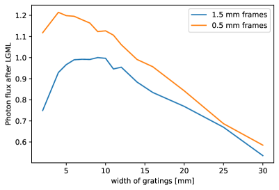
Figure 5: Effective area for an instrument filled with CAT gratings of different dimensions. In all simulations, the CAT gratings are 30 mm long in dispersion direction, but the width of the grating in cross-dispersion direction differs. When using larger gratings, there is less obscuration by frames and grating holders, but gratings deviate more from the ideal surface. The figure shows that gratings with dimensions of $30\times 10\;\mathrm{mm}^{2}$ perform best.

6 ALIGNMENT AND ERROR BUDGET

When the physical hardware for a mission is put together, nothing is perfect. Parts and pieces will always differ slightly in form, shape, and position from the locations assigned to them in the abstract design model. Ray-tracing is one useful method to study how much such misalignments will impact the performance of the instrument and thus to develop a table of alignment requirements. The looser the requirement can be, the cheaper and faster the process is. On the other hand, if the ray-tracing shows that certain elements need to be positioned very precisely, specific alignment procedures and tests might have to be developed.

For each alignment parameter, we study six degrees of freedom (three translations and three rotations). In practice, misalignments happen in all six degrees of freedom for all parts of the instrument at the same time. However, computational limitations prohibit us from exhaustively exploring the full parameter space. Instead, as a first phase, we treat PiSoX as a hierarchical collection of many elements (mirror shells, mirror module, CAT gratings, CAT grating assembly, all of which combine into the optics module etc.). We perform simulations for about a dozen elements and for each parameter we typically run simulations for 10-20 values. The full parameter space would thus require $20^{6*12}=5\times 10^{93}$ simulations. Instead, as a first step, we set up a perfectly aligned instrument and then vary one parameter for one element or one group of elements (e.g. the $x$ position of all gratings) at a time. Note that even a perfectly aligned instrument has some limitations that are inherent in the design, such as optical aberrations. We step through different values for each parameter, keeping all other alignments perfect, and run a simulations with 100,000 photons for each step. We inspect the results from simulations and select a value for the acceptable misalignment in each degree of freedom, e.g. the value where the effective area of the channel degrades by no more than 10%. Selecting the exact value is a trade-off with engineering concerns. In some degrees of freedom, the alignment may be easily reached by machining tolerances and thus we can chose a number that causes only a negligible degradation of performance, while in other cases, reaching a certain alignment might be very costly and thus we want to set the requirements for these parameters as loosely as possible.

The effects of different misalignments will add up in some cases. In others they may cancel each other out to some degree or combine multiplicatively. In future work, we will investigate misalignments for all parameters simultaneously. For the purpose of developing the error budget, there are other design parameters that are not technically related to mechanical alignment, but impact the performance in a similar way and can be analyzed with the same ray-trace setup. One example is the pointing jitter, which describes how uncertainties in the instrument pointing on the sky degrade the instrument performance. If the pointing direction on the sky jitters with time, photons will not always arrive on-axis. This is somewhat similar to a misaligned optics module.

In this section, we run simulations varying one degree of freedom at a time. Parameters that are not mechanical misalignments, such as the pointing jitter, are shown in plots with a blue background in the coming figures. Simulations for mechanical misalignments come in two flavors. Either an entire set of objects is moved deterministicly (e.g. all gratings in the grating assembly are moved 1 mm to the right) or a number of objects are moved randomly (e.g. all gratings in the grating assembly are moved along the $x$-axis, but for each grating a new number is drawn from a Gaussian distribution with $\sigma=1$ mm). The first case is shown with a gray background, the latter case is shown with a light red background. Results for all mechanical tolerancing are shown as sets of six plots. The upper row presents results from translations along the $x$, $y$, and $z$-axis, the bottom row rotations. The center of the rotation is typically the center of an element. The coordinate system for the instrument places the optical axis along the $z$-axis with photons coming in from $z=+\infty$. The origin of the coordinate system is at the nominal focal point of the mirror system. The dispersion direction of the gratings is along the positive $y$-axis. Thus, the long axis of the ML mirror is also parallel to the $y$-axis.

6.1 Pointing and mirror

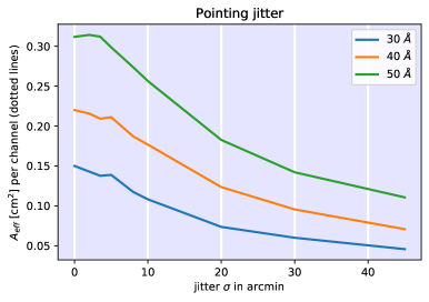
Figure 6: Change of effective area with increasing pointing jitter.

Figure 6 shows simulations using an unsteady pointing. The average pointing direction is on-axis, but the pointing jitters around that. For each photon, the true pointing direction is drawn from a Gaussian with the $\sigma$ given in the figure. This jitter represents uncertainty in the pointing, which can come from different sources, such as limited resolution of the star trackers, motion of the pointing within the time period of reading out the star trackers or integration time of the zero-order image (if used to determine the target coordinates), or the spacecraft not correcting a pointing drift fast enough.

The effective area $A_{\mathrm{eff}}$ drops with increasing jitter, because the diffracted photons do not hit the ML at the position of the Bragg peak when the target is not at a nominal position, and thus the reflectivity is lower. The drop becomes important for a jitter above a few arcminutes. Mispointing along the direction of diffraction has a much stronger effect than perpendicular to it. This is investigated in figure 7.

Figure 7: Change of effective area for observations where the target is positioned offset from the nominal pointing direction.

The modulation factor changes only marginally when the source is observed offset from the nominal position. However, as explained for the simulations with the pointing jitter above, the effective area drops dramatically when the source moves along the axis of the ML, because that means that photons will no longer arrive at the position where the spacing of the ML matches the required number given the angle and wavelength of the photon.

6.2 CAT gratings

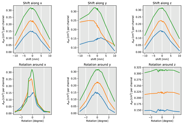
Figure 8: Change of effective area for globally misaligned CAT grating module.

Figure 8 shows simulations that move the CAT grating module as a whole, i.e. translation in $z$ means that all gratings of both sectors are moved up or down together. This particular case changes the distance between the gratings and the focal plane and thus photons will hit the ML mirror on a different location. Changes of more than a few mm will cause the photons to miss the position of the Bragg peak on the ML mirror and thus reduce $A_{\mathrm{eff}}$. The layout is insensitive to translations in $y$ (along the dispersion direction). This is the long direction of the CAT gratings and CAT gratings are tilted only ever so slightly, so that the point of intersection is essentially constant. $A_{\mathrm{eff}}$ only begins to drop when gratings moved so far that some fraction of the beam no longer hit a grating. A shift along $x$ is a shift along the stair-stepped direction. Shifts along $x$ reduce $A_{\mathrm{eff}}$ for the same reason that the layout is stair-stepped in the first place: Since photons come in at a different angle, they need to be diffracted at a different distance from the ML to hit the ML mirror at the Bragg peak.

For the rotation simulations, the origin of the rotation is the point where the optical axes intersects the “stair” surface on which the gratings are positioned. Of all the rotations, only rotations around the $y$ direction (the dispersion axis) have limits tighter than a degree or so, because rotation around $y$ changes the $z$ position of the gratings, so the effect is similar to a translation in $z$.

6.3 CAT gratings

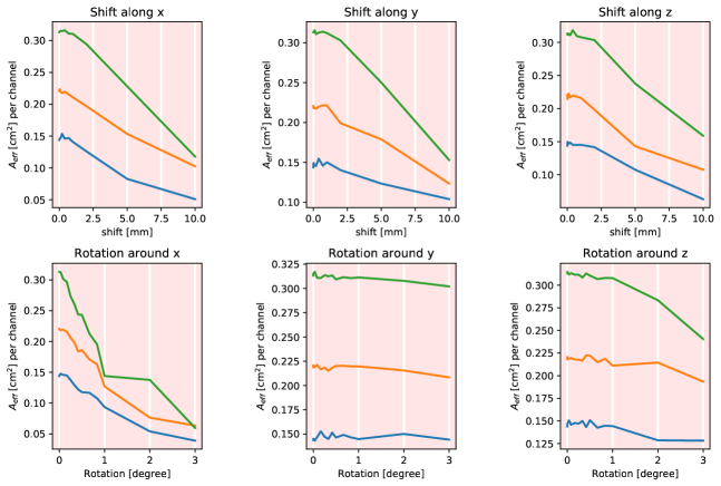
Figure 9: Change of effective area for CAT gratings misaligned with respect to each other.

Figure 9 presents simulations where individual CAT gratings are moved with respect to their nominal position on the CAT gratings assembly. All translations allow $1\sigma$ errors of a few mm, which is much larger than the size of the holder the gratings are placed in. This is a trivial constraint. Similarly, only rotations around $x$ (the short axis of the gratings) are tighter than 2 degrees. Rotations around $x$ makes the incoming photons hit the CAT gratings at an angle different from the design blaze angle and reduce the fraction of photons that are dispersed into the first order. Since photons in other orders are not reflected from the ML mirror onto the detector, this reduces the $A_{\mathrm{eff}}$ of the system. To keep the loss of $A_{\mathrm{eff}}$ below 10%, the gratings need to be positioned within 10 arcmin of the nominal rotation angle.

A change in the period of the gratings will also diffract photons to the wrong locations, but the lithography process used to manufacture the gratings gives a repeatability of the grating period that is orders of magnitude better than the PiSoX requirement.

6.4 ML mirror

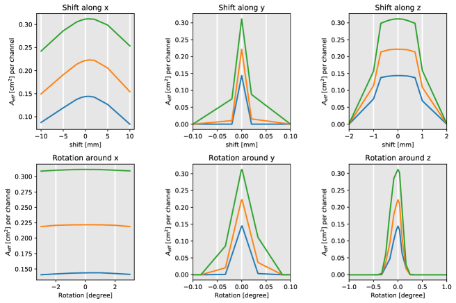
Figure 10: Change of effective area in case of a misaligned ML mirror.

The ML mirror is the most critical part of the alignment because photons have to hit the multilayer at the position of the Bragg peak. Because of this, shifts along the $y$ direction (the direction in which the multilayer is graded) are most sensitive (Figure 10) and have to be aligned to better than 10 micron. However, this is for a source at nominal position. Moving the source to a slightly off-axis position also changes where photons interact with the ML mirror. Thus, in practice, this alignment does not have to be performed to the 10 micron level for a single-channel instrument. Instead sources can just be observed slightly off-axis to compensate for any alignment error. This requires calibrating the alignment in space by observing a source at different positions, until the signal in the polarimetry channel is maximised. In this case, the instrument can no longer rotate around the nominal axis to probe different polarization angles. Instead, it has to rotate such that the source is kept at the new position determined in the calibration. On the other hand, tolerances for the other translations are a lot more relaxed – around a mm or so.

When there are two polarimetry channels, there is generally an offset position that will provide a match of the dispersed spectrum to the MLs of both channels because the effective area is so insensitive to cross-dispersion shifts. For three detectors, a suitable shift may not be possible, requiring that ground calibration properly align at least two of the ML mirrors to each other.

Rotations around the long axis of the ML mirror ($x$ axis of the coordinate system) have a very large tolerance of a few degrees. Because the physical dimensions of the mirror are small, the point of intersection with the mirror surface does not change much and thus the photons still interact with the mirror very close to position of the Bragg peak. On the other hand, rotations around the other two axes move the mirror by a significant amount. That means that the photons travel either too far or too little in $x$ direction, which causes them to miss the position of the Bragg peak and consequently reduces $A_{\mathrm{eff}}$ significantly.

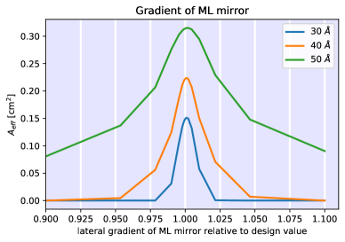
Figure 11: Change of effective area for ML mirrors where the lateral grading differs from the design gradient.

Another way for photons to miss the position of the Bragg peak is when the lateral grading of the ML mirror does not match the gradient that was assumed when placing the CAT gratings. Figure 11 shows that the gradient has to be within about 1% of the design value.

6.5 Detectors

The exact position of the detectors is not important as long as the signal still hits the detectors. With increasing misalignment, the spectral resolution of the polarimetry channel will degrade slightly. Background also increases when the extraction region size needs to be increased, but again, the background is negligible and the effect of increasing the extraction region size is negligible for any misalignment that can reasonably be expected in the focal plane.

7 SUMMARY

One viable concept for a soft X-ray polarimeter is based on CAT gratings and a multi-layer mirror. We show ray-traces for an instrument designed for a small orbital mission with a focal length of 1.25 m and a single polarimetry channel. However, our results are easily generalizable to additional channels, since each channel acts essentially as its own instrument with separate CAT gratings, ML mirrors, and detectors. We show the effective area and modulation factor based on this design.

Gratings need to be bent to match the blaze angle in a converging beam. We study different bending strategies and find that bending is required, but the performance shows negligible sensitivity to the exact value of the radius, so that only one type of grating holder with the same radius for all gratings is sufficient, simplifying design and handling. The requirement to place all gratings such that diffracted rays hit the ML mirror at the position of the Bragg peak limits the sizes of the CAT gratings. We find that a width of 10 mm optimizes performance.

Finally, we discuss alignment tolerances for all components. In most degrees of freedom the requirements are so loose that they are well below machining tolerances. However, the ML mirror has to be positioned to 10 $\mu$m in the dispersion direction relative to zeroth order, which can be calibrated and offset in flight.

- [1] Marshall, H. L., Günther, H. M., Heilmann, R. K., Schulz, N. S., Egan, M., Hellickson, T., Heine, S. N. T., Windt, D. L., Gullikson, E. M., Ramsey, B., Tagliaferri, G., and Pareschi, G., “Design of a broadband soft x-ray polarimeter,” Journal of Astronomical Telescopes, Instruments, and Systems 4, 011005 (January 2018).
- [2] Novick, R., Weisskopf, M. C., Berthelsdorf, R., Linke, R., and Wolff, R. S., “Detection of X-Ray Polarization of the Crab Nebula,” ApJL 174, L1 (May 1972).
- [3] Weisskopf, M. C., Silver, E. H., Kestenbaum, H. L., Long, K. S., and Novick, R., “A precision measurement of the X-ray polarization of the Crab Nebula without pulsar contamination.,” Astrophysical Journal Letters 220, L117–L121 (March 1978).
- [4] Weisskopf, M. C., Ramsey, B., O’Dell, S., Tennant, A., Elsner, R., Soffitta, P., Bellazzini, R., Costa, E., Kolodziejczak, J., Kaspi, V., Muleri, F., Marshall, H., Matt, G., and Romani, R., “The Imaging X-ray Polarimetry Explorer (IXPE),” in [Space Telescopes and Instrumentation 2016: Ultraviolet to Gamma Ray ], den Herder, J.-W. A., Takahashi, T., and Bautz, M., eds., Society of Photo-Optical Instrumentation Engineers (SPIE) Conference Series 9905, 990517 (July 2016).
- [5] Günther, H. M., Egan, M., Heilmann, R. K., Heine, S. N. T., Hellickson, T., Frost, J., Marshall, H. L., Schulz, N. S., and Theriault-Shay, A., “REDSoX: Monte-Carlo ray-tracing for a soft x-ray spectroscopy polarimeter,” in [Society of Photo-Optical Instrumentation Engineers (SPIE) Conference Series ], Society of Photo-Optical Instrumentation Engineers (SPIE) Conference Series 10399, 1039917 (August 2017).
- [6] Heilmann, R. K., Ahn, M., Bruccoleri, A., Chang, C.-H., Gullikson, E. M., Mukherjee, P., and Schattenburg, M. L., “Diffraction efficiency of 200-nm-period critical-angle transmission gratings in the soft x-ray and extreme ultraviolet wavelength bands,” Appl. Opt. 50, 1364–1373 (Apr 2011).
- [7] Heilmann, R. K., Bruccoleri, A. R., and Schattenburg, M. L., “High-efficiency blazed transmission gratings for high-resolution soft x-ray spectroscopy,” in [Society of Photo-Optical Instrumentation Engineers (SPIE) Conference Series ], Society of Photo-Optical Instrumentation Engineers (SPIE) Conference Series 9603, 960314 (September 2015).
- [8] Heilmann, R. K., Bruccoleri, A. R., Song, J., DeRoo, C., Cheimetz, P., Hertz, E., Smith, R. a. K., Burwitz, V., Hartner, G., La Caria, M.-M., Pelliciari, C., Guenther, H. M., Heine, S. N. T., LaMarr, B., Marshall, H. L., Schulz, N. S., Gullikson, E. M., and Schattenburg, M. L., “Blazed transmission grating technology development for the Arcus x-ray spectrometer explorer,” in [Space Telescopes and Instrumentation 2018: Ultraviolet to Gamma Ray ], den Herder, J.-W. A., Nikzad, S., and Nakazawa, K., eds., Society of Photo-Optical Instrumentation Engineers (SPIE) Conference Series 10699, 106996D (July 2018).
- [9] Heilmann, R. K., Bruccoleri, A. R., Song, J., and Schattenburg, M. L., “Progress in x-ray critical-angle transmission grating technology development,” in [Optics for EUV, X-Ray, and Gamma-Ray Astronomy IX ], Society of Photo-Optical Instrumentation Engineers (SPIE) Conference Series 11119, 1111913 (September 2019).
- [10] Günther, H. M., Frost, J., and Theriault-Shay, A., “MARXS: A Modular Software to Ray-trace X-Ray Instrumentation,” Astronomical Journal 154, 243 (Dec 2017).
- [11] Günther, H. M., Frost, J., and Theriault-Shay, A., “Chandra-marx/marxs: v1.2,” (July 2017).
- [12] Günther, H. M. and Heilmann, R. K., “Design progress on the Lynx soft x-ray critical-angle transmission grating spectrometer,” in [UV, X-Ray, and Gamma-Ray Space Instrumentation for Astronomy XXI ], Society of Photo-Optical Instrumentation Engineers (SPIE) Conference Series 11118, 111181C (September 2019).
- [13] Günther, H. M., DeRoo, C., Heilmann, R. K., Hertz, E., Smith, R. K., and Wilms, J., “Ray-tracing Arcus in phase A,” in [Space Telescopes and Instrumentation 2018: Ultraviolet to Gamma Ray ], den Herder, J.-W. A., Nikzad, S., and Nakazawa, K., eds., Society of Photo-Optical Instrumentation Engineers (SPIE) Conference Series 10699, 106996F (July 2018).
- [14] Heine, S. N. T., Marshall, H. L., Heilmann, R. K., Schulz, N. S., Beeks, K., Drake, F., Gaines, D., Levey, S., Windt, D. L., and Gullikson, E. M., “Laboratory progress in soft x-ray polarimetry,” in [Optics for EUV, X-Ray, and Gamma-Ray Astronomy VIII ], O’Dell, S. L. and Pareschi, G., eds., 10399, 245 – 252, International Society for Optics and Photonics, SPIE (2017).
- [15] Song, J., Heilmann, R. K., Bruccoleri, A. R., Hertz, E., and Schattenburg, M. L., “Metrology for quality control and alignment of CAT grating spectrometers ,” in [Space Telescopes and Instrumentation 2018: Ultraviolet to Gamma Ray ], den Herder, J.-W. A., Nikzad, S., and Nakazawa, K., eds., 10699, 146 – 157, International Society for Optics and Photonics, SPIE (2018).
- [16] Garner, A., Marshall, H. L., Heine, S. N. T., Heilmann, R. K., Song, J., Schulz, N. S., LaMarr, B. J., and Egan, M., “Component testing for x-ray spectroscopy and polarimetry,” in [UV, X-Ray, and Gamma-Ray Space Instrumentation for Astronomy XXI ], Siegmund, O. H., ed., 11118, 309 – 320, International Society for Optics and Photonics, SPIE (2019).
- [17] Marshall, H. L., Schulz, N. S., Windt, D. L., Gullikson, E. M., Craft, M., Blake, E., and Ross, C., “The use of laterally graded multilayer mirrors for soft x-ray polarimetry,” in [Optics for EUV, X-Ray, and Gamma-Ray Astronomy VII ], O’Dell, S. L. and Pareschi, G., eds., 9603, 334 – 341, International Society for Optics and Photonics, SPIE (2015).
- [18] Koyama, K., Tsunemi, H., Dotani, T., Bautz, M. W., Hayashida, K., Tsuru, T. G., Matsumoto, H., Ogawara, Y., Ricker, G. R., Doty, J., Kissel, S. E., Foster, R., Nakajima, H., Yamaguchi, H., Mori, H., Sakano, M., Hamaguchi, K., Nishiuchi, M., Miyata, E., Torii, K., Namiki, M., Katsuda, S., Matsuura, D., Miyauchi, T., Anabuki, N., Tawa, N., Ozaki, M., Murakami, H., Maeda, Y., Ichikawa, Y., Prigozhin, G. Y., Boughan, E. A., Lamarr, B., Miller, E. D., Burke, B. E., Gregory, J. A., Pillsbury, A., Bamba, A., Hiraga, J. S., Senda, A., Katayama, H., Kitamoto, S., Tsujimoto, M., Kohmura, T., Tsuboi, Y., and Awaki, H., “X-Ray Imaging Spectrometer (XIS) on Board Suzaku,” Publications of the Astronomical Society of Japan 59, 23–33 (January 2007).
- [19] Bautz, M. W., Miller, E. D., Sanders, J. S., Arnaud, K. A., Mushotzky, R. F., Porter, F. S., Hayashida, K., Henry, J. P., Hughes, J. P., Kawaharada, M., Makashima, K., Sato, M., and Tamura, T., “Suzaku Observations of Abell 1795: Cluster Emission to r200,” Publications of the Astronomical Society of Japan 61, 1117 (Oct. 2009).
- [20] Astropy Collaboration, Robitaille, T. P., Tollerud, E. J., Greenfield, P., Droettboom, M., Bray, E., Aldcroft, T., Davis, M., Ginsburg, A., Price-Whelan, A. M., Kerzendorf, W. E., Conley, A., Crighton, N., Barbary, K., Muna, D., Ferguson, H., Grollier, F., Parikh, M. M., Nair, P. H., Günther, H. M., Deil, C., Woillez, J., Conseil, S., Kramer, R., Turner, J. E. H., Singer, L., Fox, R., Weaver, B. A., Zabalza, V., Edwards, Z. I., Azalee Bostroem, K., Burke, D. J., Casey, A. R., Crawford, S. M., Dencheva, N., Ely, J., Jenness, T., Labrie, K., Lim, P. L., Pierfederici, F., Pontzen, A., Ptak, A., Refsdal, B., Servillat, M., and Streicher, O., “Astropy: A community Python package for astronomy,” Astronomy and Astrophysics 558, A33 (October 2013).
- [21] Astropy Collaboration, Price-Whelan, A. M., Sipőcz, B. M., Günther, H. M., Lim, P. L., Crawford, S. M., Conseil, S., Shupe, D. L., Craig, M. W., Dencheva, N., Ginsburg, A., VanderPlas, J. T., Bradley, L. D., Pérez-Suárez, D., de Val-Borro, M., Aldcroft, T. L., Cruz, K. L., Robitaille, T. P., Tollerud, E. J., Ardelean, C., Babej, T., Bach, Y. P., Bachetti, M., Bakanov, A. V., Bamford, S. P., Barentsen, G., Barmby, P., Baumbach, A., Berry, K. L., Biscani, F., Boquien, M., Bostroem, K. A., Bouma, L. G., Brammer, G. B., Bray, E. M., Breytenbach, H., Buddelmeijer, H., Burke, D. J., Calderone, G., Cano Rodríguez, J. L., Cara, M., Cardoso, J. V. M., Cheedella, S., Copin, Y., Corrales, L., Crichton, D., D’Avella, D., Deil, C., Depagne, É., Dietrich, J. P., Donath, A., Droettboom, M., Earl, N., Erben, T., Fabbro, S., Ferreira, L. A., Finethy, T., Fox, R. T., Garrison, L. H., Gibbons, S. L. J., Goldstein, D. A., Gommers, R., Greco, J. P., Greenfield, P., Groener, A. M., Grollier, F., Hagen, A., Hirst, P., Homeier, D., Horton, A. J., Hosseinzadeh, G., Hu, L., Hunkeler, J. S., Ivezić, Ž., Jain, A., Jenness, T., Kanarek, G., Kendrew, S., Kern, N. S., Kerzendorf, W. E., Khvalko, A., King, J., Kirkby, D., Kulkarni, A. M., Kumar, A., Lee, A., Lenz, D., Littlefair, S. P., Ma, Z., Macleod, D. M., Mastropietro, M., McCully, C., Montagnac, S., Morris, B. M., Mueller, M., Mumford, S. J., Muna, D., Murphy, N. A., Nelson, S., Nguyen, G. H., Ninan, J. P., Nöthe, M., Ogaz, S., Oh, S., Parejko, J. K., Parley, N., Pascual, S., Patil, R., Patil, A. A., Plunkett, A. L., Prochaska, J. X., Rastogi, T., Reddy Janga, V., Sabater, J., Sakurikar, P., Seifert, M., Sherbert, L. E., Sherwood-Taylor, H., Shih, A. Y., Sick, J., Silbiger, M. T., Singanamalla, S., Singer, L. P., Sladen, P. H., Sooley, K. A., Sornarajah, S., Streicher, O., Teuben, P., Thomas, S. W., Tremblay, G. R., Turner, J. E. H., Terrón, V., van Kerkwijk, M. H., de la Vega, A., Watkins, L. L., Weaver, B. A., Whitmore, J. B., Woillez, J., Zabalza, V., and Astropy Contributors, “The Astropy Project: Building an Open-science Project and Status of the v2.0 Core Package,” Astronomical Journal 156, 123 (September 2018).
- [22] van der Walt, S., Colbert, S. C., and Varoquaux, G., “The NumPy Array: A Structure for Efficient Numerical Computation,” Computing in Science and Engineering 13, 22–30 (March 2011).
- [23] Pérez, F. and Granger, B. E., “IPython: a system for interactive scientific computing,” Computing in Science and Engineering 9, 21–29 (May 2007).
- [24] Ramachandran, P. and Varoquaux, G., “Mayavi: 3D Visualization of Scientific Data,” Computing in Science & Engineering 13(2), 40–51 (2011).
- [25] Hunter, J. D., “Matplotlib: A 2D Graphics Environment,” Computing in Science and Engineering 9, 90–95 (May 2007).