Revisiting Rainbow: Promoting more Insightful and Inclusive Deep Reinforcement Learning Research

Abstract

Since the introduction of DQN, a vast majority of reinforcement learning research has focused on reinforcement learning with deep neural networks as function approximators. New methods are typically evaluated on a set of environments that have now become standard, such as Atari 2600 games. While these benchmarks help standardize evaluation, their computational cost has the unfortunate side effect of widening the gap between those with ample access to computational resources, and those without. In this work we argue that, despite the community’s emphasis on large-scale environments, the traditional small-scale environments can still yield valuable scientific insights and can help reduce the barriers to entry for underprivileged communities. To substantiate our claims, we empirically revisit the paper which introduced the Rainbow algorithm (Hessel et al., 2018) and present some new insights into the algorithms used by Rainbow.

1 Introduction

Since the introduction of DQN (Mnih et al., 2015) reinforcement learning has witnessed a dramatic increase in research papers (Henderson et al., 2018). A large portion of these papers propose new methods that build on the original DQN algorithm and network architecture, often adapting methods introduced before DQN to work well with deep networks (e.g., (van Hasselt et al., 2016; Bacon et al., 2017; Castro, 2020)). New methods are typically evaluated on a set of environments that have now become standard, such as the Atari 2600 games made available in the Arcade Learning Environment (ALE) (Bellemare et al., 2012) and the control tasks available in MuJoCo and DM control suites (Todorov et al., 2012; Tassa et al., 2020).

While these benchmarks have helped to evaluate new methods in a standardized manner, they have also implicitly established a minimum amount of computing power in order to be recognized as valid scientific contributions. Although classic reinforcement learning tasks such as MountainCar, CartPole, Acrobot, and grid worlds have not gone away, they are now used mostly for evaluating theoretical contributions (e.g., (Nachum et al., 2019; Lyle et al., 2019)); indeed, in our experience it is quite difficult to have a paper proposing a new reinforcement learning method accepted at one of the major machine learning conferences unless it includes experiments with one of the benchmarks just mentioned. This is unfortunate, as the low computational cost and speed at which one can train on small-scale environments enables broad hyper-parameter sweeps and more thorough investigations into the nuances of the methods being considered, as well as the reevaluation of certain empirical choices that have become “folk wisdom” in these types of experiments.

Furthermore, at a time when efforts such as Black in AI and LatinX in AI are helping bring people from underrepresented (and typically underprivileged) segments of society into the research community, these newcomers are faced with enormous computational hurdles to overcome if they wish to be an integral part of said community.

It thus behooves the reinforcement learning research community to incorporate a certain degree of flexibility and creativity when proposing and evaluating new research; of course, this should not be at the expense of scientific rigour. This paper is partly a position paper, partly an empirical evaluation. We argue for a need to change the status-quo in evaluating and proposing new research to avoid exacerbating the barriers to entry for newcomers from underprivileged communities. In section 4 we complement this argument by revisiting the Rainbow algorithm (Hessel et al., 2018), which proposed a new state of the art algorithm by combining a number of recent advances, on a set of small- and medium-sized tasks. This allows us to conduct a “counterfactual” analysis: would Hessel et al. (2018) have reached the same conclusions if they had run on the smaller-scale experiments we investigate here? In section 5 we extend this analysis by investigating the interaction between the different algorithms considered and the network architecture used, varying the distribution parameterization and bootstrapping methodology, and the base loss used by DQN. Finally, in section 6 we compare the Rainbow variants we considered, as well as provide insights into the properties of the different environments used in our study.

2 Preliminaries

Reinforcement learning methods are used for learning how to act (near) optimally in sequential decision making problems in uncertain environments. In the most common scenario, an agent transitions between states in an environment by making action choices at discrete time steps; upon performing an action, the environment produces a numerical reward and transitions the agent to a new state. This is formalized as a Markov decision process (Puterman, 1994) $\langle\mathcal{S},\mathcal{A},\mathcal{R},\mathcal{P},\gamma\rangle$, where $\mathcal{S}$ is a finite set of states, $\mathcal{A}$ is a finite set of actions, $\mathcal{R}:\mathcal{S}\times\mathcal{A}\rightarrow[R_{min},R_{max}]$ is the reward function, $\mathcal{P}:\mathcal{S}\times\mathcal{A}\rightarrow\Delta(\mathcal{S})$ is the transition function, where $\Delta(X)$ denotes the set of probability distributions over a set $X$, and $\gamma\in[0,1)$ is a horizon discount factor.

An agent’s behaviour is formalized as a policy $\pi:\mathcal{S}\rightarrow\Delta(\mathcal{A})$ which induces a value function $V^{\pi}:\mathcal{S}\rightarrow\mathbb{R}$:

$$V^{\pi}(s) :=\mathbb{E}\left[\sum_{t=0}^{\infty}\gamma^{t}\mathcal{R}(s_{t},a_{t})|s_{0}=s,s_{t},a_{t}\right]$$

$$=\mathbb{E}_{a\sim\pi(s)}\left[\mathcal{R}(s,a)+\gamma\mathbb{E}_{s^{\prime}\sim\mathcal{P}(s,a)}V^{\pi}(s^{\prime})\right],$$

where $s_{t}\sim\mathcal{P}(s_{t-1},a_{t-1})$ and $a_{t}\sim\pi(s_{t})$. The second line is the well-known Bellman recurrence. It is also convenient to consider the value of actions that differ from those encoded in $\pi$ via the function $Q^{\pi}:\mathcal{S}\times\mathcal{A}\rightarrow\mathbb{R}$: $Q^{\pi}(s,a):=\mathcal{R}(s,a)+\gamma\mathbb{E}_{s^{\prime}\sim\mathcal{P}(s,a)}V^{\pi}(s^{\prime})$.

It is well known that there exist policies $\pi^{*}$ that are optimal in the sense that $V^{*}(s):=V^{\pi^{*}}(s)\geq V^{\pi}(s)$ for all policies $\pi$ and states $s\in\mathcal{S}$. In reinforcement learning we are typically interested in having agents find these policies by interacting with the environment. One of the most popular ways to do so is via $Q$-learning, where an agent maintains a function $Q_{\theta}$, parameterized by $\theta$ (e.g. the weights in a neural network), and updates it after observing the transition $s\overset{a,r}{\rightarrow}s^{\prime}$ using the method of temporal differences (Sutton, 1988):

$$Q_{\theta}(s,a)\leftarrow Q_{\theta}(s,a)+\alpha\left(Q^{*}(s^{\prime},a^{\prime})-Q_{\theta}(s,a)\right)$$ (1)

where $\alpha$ is a learning rate and the optimal target values $Q^{*}(s^{\prime},a^{\prime})=r+\gamma\max_{a^{\prime}\in\mathcal{A}}Q_{\theta}(s^{\prime},a^{\prime})$

2.1 DQN

Mnih et al. (2015) introduced DQN, which combined Q-learning with deep networks. Some of the most salient design choices are:

• The $Q$ function is represented using a feed forward neural network consisting of three convolutional layers followed by two fully connected layers. Two copies of the $Q$-network are maintained: an online network (parameterized by $\theta$) and a target network (parameterized by $\bar{\theta}$). The online network is updated via the learning process described below, while the target network remains fixed and is synced with the online weights at less frequent (but regular) intervals.

• A large replay buffer $D$ is maintained to store experienced transitions $(s,a,r,s^{\prime})$ (Lin, 1992).

• The update in Equation 1 is implemented using the following loss function to update the online network:

  $$L(\theta)=\mathbb{E}_{(s,a,r,s^{\prime})\sim U(D)}[\left(Y^{DQN}-Q_{\theta}(s,a)\right)^{2}]$$ (2)

  using $Y^{DQN}=\left(r+\gamma\max_{a^{\prime}\in\mathcal{A}}Q_{\bar{\theta}}(s^{\prime},a^{\prime})\right)$ and mini-batches of size 32.

2.2 Rainbow

In this section we briefly present the enhancements to DQN that were combined by Hessel et al. (2018) for the Rainbow agent.

Double Q-learning: van Hasselt et al. (2016) added double Q-learning (Hasselt, 2010) to mitigate overestimation bias in the $Q$-estimates by decoupling the maximization of the action from its selection in the target bootstrap.

Prioritized experience replay: Instead of sampling uniformly from the replay buffer ($U(D)$), prioritized experience replay (Schaul et al., 2016) proposed to sample a trajectory $t=(s,a,r,s^{\prime})$ with probability $p_{t}$ proportional to the temporal difference error.

Dueling networks: Wang et al. (2016) introduced dueling networks by modifying the DQN network architecture. Specifically, two streams share the initial convolutional layers, separately estimating $V^{*}(s)$, and the advantages for each action: $A(s,a):=Q^{*}(s,a)-V^{*}(s)$. The output of the network is a combination of these two streams. Multi-step learning: Instead of computing the temporal difference error using a single-step transition, one can use multi-step targets instead (Sutton, 1988), where for a trajectory $(s_{0},a_{0},r_{0},s_{1},a_{1},\cdots)$ and update horizon $n$: $R_{t}^{(n)}:=\sum_{k=0}^{n-1}\gamma^{k}r_{t+k+1}$, yielding the multi-step temporal difference: $R_{t}^{(n)}+\gamma^{n}\max_{a^{\prime}\in\mathcal{A}}Q_{\bar{\theta}}(s_{t+n},a^{\prime})-Q_{\theta}(s_{t},a_{t})$.

Distributional RL: Bellemare et al. (2017) demonstrated that the Bellman recurrence also holds for value distributions: $Z(x,a)\overset{D}{=}R(s,a)+\gamma Z(X^{\prime},A^{\prime})$, where $Z$, $R$, and $(X^{\prime},A^{\prime})$ are random variables representing the return, immediate reward, and next state-action, respectively. The authors present an algorithm (C51) to maintain an estimate $Z_{\theta}$ of the return distribution $Z$ by use of a parameterized categorical distribution with 51 atoms.

Noisy nets: Fortunato et al. (2018) propose replacing the simple $\epsilon$-greedy exploration strategy used by DQN with noisy linear layers that include a noisy stream.

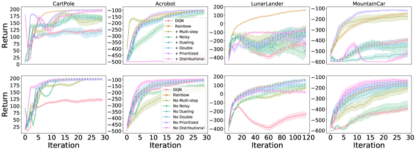
Figure 1: Comparison of the different algorithmic components on the four small environments using the optimal hyper-parameters from Table 1 for each, averaged over 100 independent runs (shaded areas show 95% confidence intervals). Top row explores adding on top of DQN, bottom row explores removing from Rainbow.

3 The cost of Rainbow

Although the value of the hybrid agent uncovered by Hessel et al. (2018) is undeniable, this result could have only come from a large research laboratory with ample access to compute. Indeed, each Atari 2600 game from the ALE (there are 57 in total) takes roughly 5 days to fully train using specialized hardware (for example, an NVIDIA Tesla P100 GPU). Additionally, in order to be able to report performance with confidence bounds it is common to use at least five independent runs (Henderson et al., 2018; Machado et al., 2018).

Thus, to provide the convincing empirical evidence for Rainbow, Hessel et al. (2018) required approximately 34,200 GPU hours (or 1425 days). Note that this cost does not include the hyper-parameter tuning that was necessary to optimize the various components. Considering that the cost of a Tesla P100 GPU is around US$6,000, providing this evidence will take an unreasonably long time as it is prohibitively expensive to have multiple GPUs in a typical academic lab so they can be used in parallel. As a reference point, the average minimum monthly wage in South America (excluding Venezuela) is approximately US$313; in other words, one GPU is the equivalent of approximately 20 minimum wages. Needless to say, this expectation is far from inclusive.

In light of this, we wish to investigate three questions:

1. Would Hessel et al. (2018) have arrived at the same qualitative conclusions, had they run their experiments on a set of smaller-scale experiments?

2. Do the results of Hessel et al. (2018) generalize well to non-ALE environments, or are their results overly-specific to the chosen benchmark?

3. Is there scientific value in conducting empirical research in reinforcement learning when restricting oneself to small- to mid-scale environments?

We investigate the first two in Section 4, and the last in Sections 5 and 6.

4 Revisiting Rainbow

4.1 Methodology

We follow a similar process as Hessel et al. (2018) in evaluating the various algorithmic variants mentioned above: we investigate the effect of adding each on top of the original DQN agent as well as the effect of dropping each from the final Rainbow agent, sweeping over learning rates for each. Our implementation is based on the Dopamine framework (Castro et al., 2018). Note that Dopamine includes a “lite” version of Rainbow, which does not include noisy networks, double DQN, nor dueling networks, but we have added all these components in our implementation.

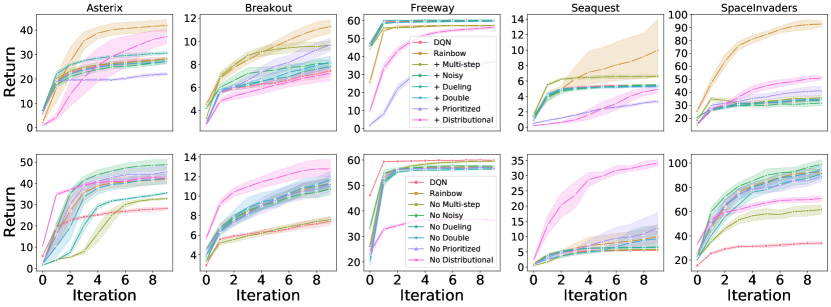
Figure 2: Comparison of the different algorithmic components on the five MinAtar games, averaged over 10 independent runs (shaded areas show 90% confidence intervals). Top row explores adding on top of DQN, bottom row explores removing from Rainbow.

We perform our empirical evaluation on small-scale environments (CartPole, Acrobot, LunarLander, and MountainCar) which are all available as part of the OpenAI Gym library (Brockman et al., 2016) (see Appendix A for a detailed description of each environment). We used multilayer perceptrons (MLPs) with 2 layers of 512 units each for these experiments. The agents were all trained on a CPU; it is worth noting that of these environments the one that took longest to train (LunarLander) is still able to finish in under two hours.

In order to strengthen the Rainbow Connection, we also ran a set of experiments on the MinAtar environment (Young and Tian, 2019), which is a set of miniaturized versions of five ALE games (Asterix, Breakout, Freeway, Seaquest, and SpaceInvaders). These environments are considerably larger than the four classic control environments previously explored, but they are significantly faster to train than regular ALE environments. Specifically, training one of these agents takes approximately 12-14 hours on a P100 GPU. For these experiments, we followed the network architecture used by Young and Tian (2019) consisting of a single convolutional layer followed by a linear layer.

4.2 Empirical evaluation

Under constant hyper-parameter settings (see appendix for details), we evaluate both the addition of each algorithmic component to DQN, as well as their removal from the full Rainbow agent on the classic control environments (Figure 1) and on Minatar (Figure 2).

We analyze our results in the context of the first two questions posed in Section 3: Would Hessel et al. (2018) have arrived at the same qualitative conclusions, had they run their experiments on a set of smaller-scale experiments? Do the results of Hessel et al. (2018) generalize well to non-ALE environments, or are their results overly-specific to the chosen benchmark?

What we find is that the performance of the different components is not uniform throughout all environments; a finding which is consistent with the results observed by Hessel et al. (2018). However, if we were to suggest a single agent that balances the tradeoffs of the different algorithmic components, our analysis would be consistent with Hessel et al. (2018): combining all components produces a better overall agent.

Nevertheless, there are important details in the variations of the different algorithmic components that merit a more thorough investigation. An important finding of our work is that distributional RL, when added on its own to DQN, may actually hurt performance (e.g. Acrobot and Freeway); similarly, performance can sometimes increase when distributional RL is removed from Rainbow (e.g. MountainCar and Seaquest); this is in contrast to what was found by Hessel et al. (2018) on the ALE experiments and warrants further investigation. As Lyle et al. (2019) noted, under non-linear function approximators (as we are using in these experiments), using distributional RL generally produces different outcomes than the non-distributional variant, but these differences are not always positive.

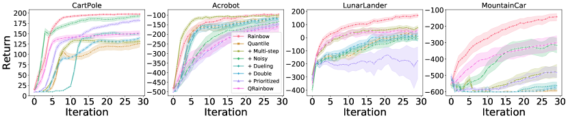
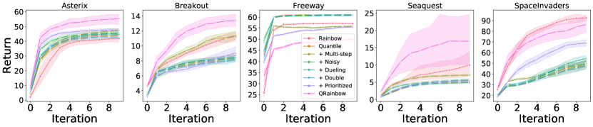
Figure 3: Investigating the combination of the different algorithmic components with QR-DQN (shaded areas show 95% (top) and 90% (bottom) confidence intervals).

5 Beyond the Rainbow

In this section we seek to answer the third question posed in section 3: Is there scientific value in conducting empirical research in small- to mid-scale environments? We leverage the low cost of the small-scale environments to conduct a thorough investigation into some of the algorithmic components studied. Unless otherwise specified, the classic control and MinAtar environments are averaged over 100 and 10 independent runs, respectively; in both cases shaded areas report 95% confidence intervals.

5.1 Examining network architectures and batch sizes

We investigated the interaction of the best per-game hyper-parameters with the number of layers and units per layer. Due to space constraints we omit the figures from the main paper, but include them in the appendix. We found that in general using 2-3 layers with at least 256 units each yielded the best performance. Further, aside from Cartpole, the algorithms were generally robust to varying network architecture dimensions.

Another often overlooked hyper-parameter in training RL agents is the batch size. We investigated the sensitivity of DQN and Rainbow to varying batch sizes and found that while for DQN it is sub-optimal to use a batch size below 64, Rainbow seems fairly robust to both small and large batch sizes.

5.2 Examining distribution parameterizations

Although distributional RL is an important component of the Rainbow agent, at the time of its development Rainbow was only evaluated with the C51 parameterization of the distribution, as originally proposed by Bellemare et al. (2017). Since then there have been a few new proposals for parameterizing the return distribution, notably quantile regression (Dabney et al., 2017, 2018a) and implicit quantile networks (Dabney et al., 2018b). In this section we investigate the interaction of these parameterizations with the other Rainbow components.

Quantile Regression for Distributional RL

In contrast to C51, QR-DQN (Dabney et al., 2017, 2018a) computes the return quantile values for $N$ fixed, uniform probabilities. Compared to C51, QR-DQN has no restrictions or bound for value, as the distribution of the random return is approximated by a uniform mixture of $N$ Diracs: $Z_{\theta}(x,a):=\frac{1}{N}\sum_{i=1}^{N}\delta_{\theta_{i}(x,a)}$, with each $\theta_{i}$ assigned a quantile value trained with quantile regression. In Figure 3 we evaluate the interaction of the different Rainbow components with Quantile and find that, in general, QR-DQN responds favourably when augmented with each of the components. We also evaluate a new agent, QRainbow, which is the same as Rainbow but with the QR-DQN parameterization. It is interesting to observe that in the classic control environments Rainbow outperforms QRainbow, but QRainbow tends to perform better than Rainbow on Minatar (with the notable exception of Freeway), suggesting that perhaps the quantile parameterization of the return distribution has greater benefits when used with networks that include convolutional layers.

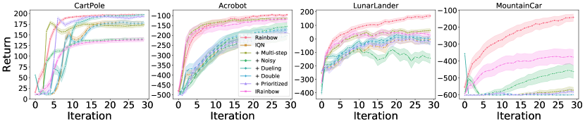
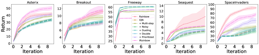
Figure 4: Investigating the combination of the different algorithmic components with IQN (shaded areas show 95% (top) and 90% (bottom) confidence intervals).

Implicit quantile networks

We continue by investigating using implicit quantile networks (IQN) as the parameterization of the return distribution Dabney et al. (2018b). IQN learns to transform a base distribution (typically a uniform distribution in $[0,1]$) to the quantile values of the return distribution. This can result in greater representation power in comparison to QR-DQN, as well as the ability to incorporate distortion risk measures. We repeat the “Rainbow experiment” with IQN and report the results in Figure 4. In contrast to QR-DQN, in the classic control environments the effect on performance of various Rainbow components is rather mixed and, as with QR-DQN IRainbow underperforms Rainbow. In Minatar we observe a similar trend as with QR-DQN: IRainbow outperforms Rainbow on all the games except Freeway.

5.3 Munchausen Reinforcement Learning

Vieillard et al. (2020) introduced Munchausen RL as a simple variant to any temporal difference learning agent consisting of two main components: the use of stochastic policies and augmenting the reward with the scaled log-policy. Integrating their proposal to DQN yields M-DQN with performance superior to that of C51; the integration of Munchausen-RL to IQN produced M-IQN, a new state-of-the art agent on the ALE.

In Figure 5 we report the results when repeating the Rainbow experiment on M-DQN and M-IQN. In the classic control environments neither of the Munchausen variants seem to yield much of an improvement over their base agents. In Minatar, while M-DQN does seem to improve over DQN, the same cannot be said of M-IQN. We explored combining all the Rainbow components with the Munchausen agents and found that, in the classic control environments, while M-Rainbow underperforms relative to its non-Munchausen counterpart, M-IRainbow can provide gains. In Minatar, the results vary from game to game, but it appears that the Munchausen agents yield an advantage on the same games (Asterix, Breakout, and SpaceInvaders).

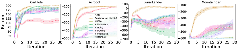
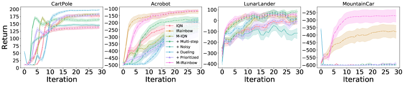
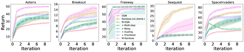
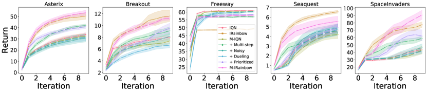
Figure 5: Investigating the combination of the different algorithmic components with M-DQN and M-IQN (shaded areas show 95% (top 2) and 90% (bottom 2) confidence intervals).

.

5.4 Reevaluating the Huber loss

The Huber loss is what is usually used to train DQN agents as it is meant to be less sensitive to outliers. Based on recent anecdotal evidence, we decided to evaluate training DQN using the mean-squared error (MSE) loss and found the surprising result that on all environments considered using the MSE loss yielded much better results than using the Huber loss, sometimes even surpassing the performance of the full Rainbow agent (full classic control and Minatar results are provided in the appendix). This begs the question as to whether the Huber loss is truly the best loss to use for DQN, especially considering that reward clipping is typically used for most ALE experiments, mitigating the occurence of outlier observations. Given that we used Adam (Kingma and Ba, 2015) for all our experiments while the original DQN algorithm used RMSProp, it is important to consider the choice of optimizer in answering this question.

To obtain an answer, we compared the performance of the Huber versus the MSE loss when used with both the Adam and RMSProp optimizers on all 60 Atari 2600 games. In Figure 6 we present the improvement obtained when using the Adam optimizer with the MSE loss over using the RMSProp optimizer with the Huber loss and find that, overwhelmingly, Adam+MSE is a superior combination than RMSProp+Huber. In the appendix we provide complete comparisons of the various optimizer-loss combinations that confirm our finding. Our analyses also show that, when using RMSProp, the Huber loss tends to perform better than MSE, which in retrospect explains why (Mnih et al., 2015) chose the Huber over the simpler MSE loss when introducing DQN.

Our findings highlight the importance in properly evaluating the interaction of the various components used when training RL agents, as was also argued by Fujimoto et al. (2020) with regards to loss functions and non-uniform sampling from the replay buffer; as well as by Hessel et al. (2019) with regards to inductive biases used in training RL agents.

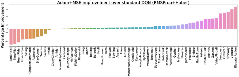
Figure 6: Comparison of training DQN using the Adam optimizer with the MSE loss, versus the Huber loss with the RMSProp. All results report the average of 5 independent runs.

6 Putting it all together

6.1 Rainbow flavours

We compare the performance of DQN against all of the Rainbow variants and show the results of two environments in Figure 7 (full comparisons in the appendix). These two environments highlight the fact that, although Rainbow does outperform DQN, there are important differences amongst the various flavours that invite further investigation.

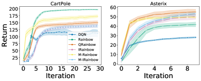
Figure 7: Comparing DQN against the various Rainbow flavours.

6.2 Environment properties

Our exhaustive experimentation on the four classic control and five MinAtar environments grant us some insight into their differing properties. We believe these environments pose a variety of interesting challenges for RL research and present a summary of our insights here, with a more thorough analysis in the appendix, in the hope that it may stimulate future investigations.

Classic control

Although CartPole is a relatively simple task, DQN can be quite sensitive to learning rates and as such, can prove an interesting testbed for optimizer stability. We found the use of Noisy networks and MSE loss to dramatically help with this sensitivity. It seems that distributional RL is required for obtaining good performance on LunarLander (see the poor results with DQN, M-DQN, and M-Rainbow in comparison with the others), suggesting this would be a good environment to investigate the differences in expectational and distributional RL as proposed by Lyle et al. (2019). Both Acrobot and MountainCar are sparse reward environments, which are typically good environments for investigating exploration strategies; indeed, we observe that Noisy networks tend to give a performance gain in both these environments. MountainCar appears to be the more difficult of the two, a fact also observed by Tang et al. (2017), Colas et al. (2018a), and Declan et al. (2020).

MinAtar

The value of MinAtar environments has already been argued by Young and Tian (2019) and recently exemplified by Ghiassian et al. (2020) and Buckman et al. (2021). It is worth highlighting that both Seaquest and Freeway appear to lend themselves well for research on exploration methods, due to their partial observability and reward sparsity. We would like to stress that these environments enable researchers to investigate the importance and effect of using convolutional networks in RL without the prohibitive expense of the ALE benchmark.

7 Conclusion

On a limited computational budget we were able to reproduce, at a high-level, the findings of Hessel et al. (2018) and uncover new and interesting phenomena. Evidently it is much easier to revisit something than to discover it in the first place; however, our intent with this work was to argue for the relevance and significance of empirical research on small- and medium-scale environments. We believe that these less computationally intensive environments lend themselves well to a more critical and thorough analysis of the performance, behaviours, and intricacies of new algorithms (a point also argued by Osband et al. (2020)). It is worth remarking that when we initially ran 10 independent trials for the classic control environments, the confidence intervals were very wide and inconclusive; boosting the independent trials to 100 gave us tighter confidence intervals with small amounts of extra compute. This would be impractical for most large-scale environments. Ensuring statistical significance when comparing algorithms, a point made by Colas et al. (2018b) and Jordan et al. (2020), is facilitated with the ability to run a large number of independent trials.

We are by no means calling for less emphasis to be placed on large-scale benchmarks. We are simply urging researchers to consider smaller-scale environments as a valuable tool in their investigations, and reviewers to avoid dismissing empirical work that focuses on these smaller problems. By doing so, we believe, we will get both a clearer picture of the research landscape and will reduce the barriers for newcomers from diverse, and often underprivileged, communities. These two points can only help make our community and our scientific advances stronger.

8 Acknowledgements

The authors would like to thank Marlos C. Machado, Sara Hooker, Matthieu Geist, Nino Vieillard, Hado van Hasselt, Eleni Triantafillou, and Brian Tanner for their insightful comments on our work.

APPENDICES: Revisiting Rainbow

Appendix A Environments

For OpenAI environments, data is summarized from https://github.com/openai/gym and information provided on the wiki https://github.com/openai/gym/wiki.

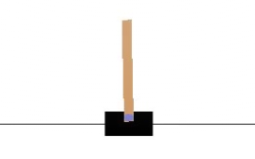
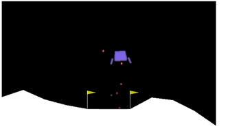
Figure 8: The classic control environments. From left to right: CartPole, Acrobot, LunarLander, and MountainCar.

A.1 CartPole-v0

CartPole is a task of balancing a pole on top of the cart. The cart has access to its position and velocity as state, and can only go left or right for each action. The task is over when the pole falls over (less than $\pm 12$ deg), the cart goes out of the boundaries ($\pm 2.4$ units off the center), or 200 time steps are reached, with each step returning 1 reward. The agent is given a continuous 4-dimensional space describing the environment, and can respond by returning one of two values, pushing the cart either right or left.

A.2 Acrobot-v1

In the Acrobot environment, the agent is given rewards for swinging a double-jointed pendulum up from a stationary position. The agent can actuate the second joint by returning one of three actions, corresponding to left, right, or no torque. The agent is given a six dimensional vector describing the environment’s angles and velocities. The episode ends when the end of the second pole is more than the length of a pole above the base. For each timestep that the agent does not reach this state, it is given a -1 reward. The episode length is 500 timesteps.

A.3 LunarLander-v2

In the LunarLander environment, the agent attempts to land a lander on a particular location on a simulated 2D world. If the lander hits the ground going too fast, the lander will explode, or if the lander runs out of fuel, the lander will plummet toward the surface. The agent is given a continuous vector describing the state, and can turn its engine on or off. The landing pad is placed in the center of the screen, and if the lander lands on the pad, it is given a reward (100-140 points). The agent also receives a variable amount of reward when coming to rest, or contacting the ground with a leg (10 points). The agent loses a small amount of reward by firing the engine (-0.3 points), and loses a large amount of reward if it crashes (-100 points). The observation consists of the x and y coordinates, the x and y velocities, angle, angular velocity, and ground contact information of the lander (left and right leg) and the action consists of do nothing, fire left orientation engine, fire down engine and fire right orientation engine.

A.4 MountainCar-v0

MountainCar is a one dimensional track between two mountains. The goal is to drive up the mountain to the right. The agent receives a -1 reward for every time step it does not reach the top. The episode terminates when it reaches 0.5 position, or if 200 iterations are reached. The objective is for the agent to learn to drive back and forth to build momentum that will be enough to push the car up the hill. The observation consists of the car’s position and velocity and the action consists of pushing left, pushing right and no push.

A.5 MinAtar Environments

Some of the best reinforcement learning algorithms require tens or hundreds of millions of timesteps to learn to play Atari games, the equivalent of several weeks of training in real time. MinAtar reduces the complexity of the representation learning problem for 5 Atari games, while maintaining the mechanics of the original games as much as possible. We use these MinAtar games to measure the impact of using some extensions to the DQN algorithm. MinAtar provides analogues to five Atari games which play out on a 10x10 grid. The environments provide a 10x10xn state representation, where each of the n channels correspond to a game-specific object, such as ball, paddle and brick in the game Breakout. Detailed descriptions of each game are available in https://github.com/kenjyoung/MinAtar.

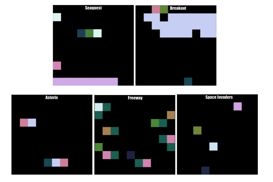
Figure 9: Visualization of each MinAtar environment.

Appendix B Detailed description of the revisting rainbow components

In this section we present the enhancements to DQN that were combined for the revisting rainbow agent.

B.1 Double Q-learning

van Hasselt et al. [2016] added double Q-learning [Hasselt, 2010] to mitigate overestimation bias in the $Q$-estimates by decoupling the maximization of the action from its selection in the target bootstrap. The loss from Equation 2 is replaced with

$$L(\theta)=\mathbb{E}_{(s,a,r,s^{\prime})\sim U(D)}\left[\left(r+\gamma Q_{\bar{\theta}}(s^{\prime},\arg\max_{a^{\prime}\in\mathcal{A}}Q_{\theta}(s^{\prime},a^{\prime}))-Q_{\theta}(s,a)\right)^{2}\right]$$

B.2 Prioritized experience replay

Instead of sampling uniformly from the replay buffer ($U(D)$), prioritized experience replay [Schaul et al., 2016] proposed to sample a trajectory $t=(s,a,r,s^{\prime})$ with probability $p_{t}$ proportional to the temporal difference error:

$$p_{t}\propto\left|r+\gamma\max_{a^{\prime}\in\mathcal{A}}Q_{\bar{\theta}}(s^{\prime},a^{\prime})-Q_{\theta}(s,a)\right|^{\omega}$$

where $\omega$ is a hyper-parameter for the sampling distribution.

B.3 Dueling networks

Wang et al. [2016] introduced dueling networks by modifying the DQN network architecture. Specifically, two streams share the initial convolutional layers, separately estimating $V^{*}(s)$, and the advantages for each action: $A(s,a):=Q^{*}(s,a)-V^{*}(s)$. The output of the full network is defined by:

$$Q_{\theta}(s,a)=V_{\eta}(f_{\eta}(s))+A_{\psi}(f_{\eta}(s),a)-\frac{\sum_{a^{\prime}\in\mathcal{A}}A_{\psi}(f_{\xi}(s),a^{\prime})}{|\mathcal{A}|}$$

Where $\xi$ denotes the parameters for the shared convolutional layers, $\eta$ denotes the parameters for the value estimator stream, $\psi$ denots the parameters for the advantage estimator stream, and $\theta:=\xi\cup\eta\cup\psi$.

B.4 Multi-step learning

Instead of computing the temporal difference error using a single-step transition, one can use multi-step targets instead [Sutton, 1988], where for a trajectory $(s_{0},a_{0},r_{0},s_{1},a_{1},\cdots)$ and update horizon $n$:

$$R_{t}^{(n)}:=\sum_{k=0}^{n-1}\gamma^{k}r_{t+k+1}$$

yielding the multi-step temporal difference:

$$R_{t}^{(n)}+\gamma^{n}\max_{a^{\prime}\in\mathcal{A}}Q_{\bar{\theta}}(s_{t+n},a^{\prime})-Q_{\theta}(s_{t},a_{t})$$

B.5 Distributional RL

Bellemare et al. [2017] demonstrated that the Bellman recurrence also holds for value distributions:

$$Z(x,a)\overset{D}{=}R(s,a)+\gamma Z(X^{\prime},A^{\prime})$$

where $Z$, $R$, and $(X^{\prime},A^{\prime})$ are random variables representing the return, immediate reward, and next state-action, respectively. The authors present an algorithm (C51) to maintain an estimate $Z_{\theta}$ of the return distribution $Z$ by use of a parameterized categorical distribution with 51 atoms.

B.6 Quantile Regression for Distributional RL

Dabney et al. [2017] computes the return quantile values for $N$ fixed, uniform probabilities. The distribution of the random return is approximated by a uniform mixture of $N$ Diracs with each $\theta_{i}$ assigned a quantile value trained with quantile regression. Formally, a quantile distribution $Z_{\theta}\in\mathcal{Z}_{Q}$ maps each state-action pair $(x,a)$ to a uniform probability distribution is,

$$Z_{\theta}(x,a):=\frac{1}{N}\sum_{i=1}^{N}\delta_{\theta_{i}(x,a)}$$

These quantile estimates are trained using the Huber [Huber, 1964] quantile regression loss.

B.7 Implicit quantile networks

Dabney et al. [2018b] extend the approach of Dabney et al.(2018), from learning a discrete set of quantiles to learningthe full quantile function, a continuous map from probabilities to returns. Moreover, extended the fixed quantile fractions to uniform samples. The approximation of the quantile function $Z$ is,

$$Z_{\tau}(x,a)\approx f(\psi(x)\odot\phi(\tau))_{a}$$

where $\odot$ denotes the element-wise (Hadamard) product.

B.8 Noisy nets

Fortunato et al. [2018] propose replacing the simple $\epsilon$-greedy exploration strategy used by DQN with noisy linear layers that include a noisy stream. Specifically, the standard linear layers defined by $\mathbf{y}=\mathbf{b}+\mathbf{Wx}$ are replaced by:

$$\mathbf{y}=(\mathbf{b}+\mathbf{Wx})+(\mathbf{b_{noisy}}\odot\epsilon^{b}+(\mathbf{W_{noisy}}\odot\epsilon^{w})\mathbf{x})$$

where $\epsilon^{b}$ and $\epsilon^{w}$ are noise variables (Hessel et al. [2018] use factorised Gaussian noise) and $\odot$ is the Hadamard product.

B.9 Munchausen Reinforcement Learning

Vieillard et al. [2020] modify the regression target adding the scaled log-policy to the immediate reward:

$$Y^{M-DQN}=r_{t}+\alpha\tau\ln\pi_{\bar{\theta}}\left(a_{t}\mid s_{t}\right)+\gamma\sum_{a^{\prime}\in\mathcal{A}}\pi_{\bar{\theta}}\left(a^{\prime}\mid s_{t+1}\right)\left(Q_{\bar{\theta}}\left(s_{t+1},a^{\prime}\right)-\tau\ln\pi_{\bar{\theta}}\left(a^{\prime}\mid s_{t+1}\right)\right)$$

with $\pi_{\theta}=\operatorname{sm}\left(\frac{Q_{\bar{\theta}}}{\tau}\right)$ and a scaling factor $\alpha\in[0,1]$.

B.10 Loss functions

We ran experiments using Mean Square Error and Huber loss [Huber, 1964], therefore we consider it important to introduce these concepts in this paper. MSE is the sum of squared distances between the target variable and predicted values. MSE gives relatively higher weight (penalty) to large errors/outliers, while smoothening the gradient for smaller errors. The MSE is formally defined by the following equation,

$$\mathrm{MSE}(y_{i},\hat{y}_{i})=\frac{1}{2}\left(y_{i}-\hat{y}_{i}\right)^{2}$$

On the other hand, Huber loss is less sensitive to outliers in data than the squared error loss and it is defined by the following equation,

$$\mathrm{Huber}\left(y_{i},\hat{y}_{i}\right)=\left\{\begin{array}[]{lr}\frac{1}{2}\left(y_{i}-\hat{y}_{i}\right)^{2}&\text{ for }\left|y_{i}-\hat{y}_{i}\right|\leq\delta,\\ \delta\left|y_{i}-\hat{y}_{i}\right|-\frac{1}{2}\delta^{2}&\text{ otherwise }\end{array}\right.$$

Appendix C Hyperparameters settings for classic control environments

Table 1: Hyperparameters settings for classic control environments

Hyperparameter	DQN	Rainbow	QR-DQN	IQN	M-DQN	M-IQN
gamma	0.99	0.99	0.99	0.99	0.99	0.99
update horizon	1	3	1	1	1	1
min replay history	500	500	500	500	500	500
update period	4	2	2	2	4	2
target update period	100	100	100	100	100	100
normalize obs	True	True	True	True	True	True
hidden layer	2	2	2	2	2	2
neurons	512	512	512	512	512	512
num atoms	-	51	51	-	-	-
vmax	-	200	-	-	-	-
kappa	-	-	1	1	-	1
tau	-	-	-	-	100	0.03
alpha	-	-	-	-	1	1
clip value min	-	-	-	-	-1e3	-1
num tau samples	-	-	-	32	-	32
num tau prime samples	-	-	-	32	-	32
num quantile samples	-	-	-	32	-	32
quantile embedding dim	-	-	-	64	-	64
learning rate	0.001	0.001	0.001	0.001	0.001	0.001
eps	3.125e-4	3.125e-4	3.125e-4	3.125e-4	3.125e-4	3.125e-4
num iterations	30	30	30	30	30	30
replay capacity	50000	50000	50000	50000	50000	50000
batch size	128	128	128	128	128	128

Appendix D Hyperparameters settings for MinAtar environments

Table 2: Hyperparameters settings for MinAtar environments

Hyperparameter	DQN	Rainbow	QR-DQN	IQN	M-DQN	M-IQN
gamma	0.99	0.99	0.99	0.99	0.99	0.99
update horizon	1	3	1	1	1	1
min replay history	1000	1000	1000	1000	1000	1000
update period	4	4	4	4	4	4
target update period	1000	1000	1000	1000	1000	1000
normalize obs	True	True	True	True	True	True
num atoms	-	51	51	-	-	-
vmax	-	100	-	-	-	-
kappa	-	-	1	1	-	1
tau	-	-	-	-	0.03	0.03
alpha	-	-	-	-	0.9	0.9
clip value min	-	-	-	-	- 1	-1
num tau samples	-	-	-	32	-	32
num tau prime samples	-	-	-	32	-	32
num quantile samples	-	-	-	32	-	32
quantile embedding dim	-	-	-	64	-	64
learning rate	0.00025	0.00025	0.00025	0.00025	0.00025	0.00025
eps	3.125e-4	3.125e-4	3.125e-4	3.125e-4	3.125e-4	3.125e-4
num iterations	10	10	10	10	10	10
replay capacity	100000	100000	100000	100000	100000	100000
batch size	32	32	32	32	32	32

Appendix E Average runtime for environments used in the experiments

Table 3: Average runtime.

Figures	Average time (minutes)
Cartpole	10
Acrobot	10
LunarLander	30
MountainCar	10
MinAtar games	720
Atari games	7200

Appendix F Impact of algorithmic components

In the following tables we list the algorithmic components that had the most positive effect on the various agents and environments. The following abbreviations are used in this section: Dist: Distributional, Noi: Noisy, Prio: Prioritized, Mult: Multi-step, Dou: Double , Due: Dueling.

Table 4: Impact of algorithmic components for each agent on classic control environments.

Agent	Operation	Cartpole	Acrobot	LunarLander	MountainCar
DQN	+	Dist/Noi	Prio/ Mult	Dist/ Mult	Mult/Dou
Rainbow	-	Mult/Noi	Mult/Noi	Dist/Mult	Mult/Noi
QR-DQN	+	Noi/Prio	Mult	Mult	Noi/Mult
IQN	+	Prio /Due	Mult/Noi	Mult/Dou	Noi
M-DQN	+	Mult	Mult /Prio	Due/Noi	Mult
M-IQN	+	Prio	Mult	Mult /Due	-

Table 5: Impact of algorithmic components for each agent on MinAtar games.

Agent	Operation	Asterix	Breakout	Freeway	Seaquest	SpaceInvaders
DQN	+	Dist/Due	Mult/Dou	Due/Noi	Mult/Noi	Dist/ Mult
Rainbow	-	Dist/Mult	Mult/ Dist	Dist/Due	Mult/Due	Dist/Mult
QR-DQN	+	Prio/ Multi-step	Mult/ Prio	Noi	Mult/Noi	Prio/Due
IQN	+	Prio/Noi	Mult/Noi	Due	Mult/Due	Prio/Mult
M-DQN	+	Prio/Mult	Prio/Mult	-	Mult	Prio/Due
M-IQN	+	Mult/Prio	Prio/ Mult	-	Prio/Noi	Prio/ Mult

Table 6: The most important component for classic control environments and MinAtar games.

Agent	Operation	Classic control	MinAtar
DQN	+	Mult	Mult
Rainbow	-	Mult	Dist
QR-DQN	+	Mult	Prio
IQN	+	Mult	Mult
M-DQN	+	Mult	Prio
M-IQN	+	Mult	Prio

Table 7: The most important component for each environment.

Environment	Component
Cartpole	Prio
Acrobot	Mult
LunarLander	Mult
MountainCar	Noi
Asterix	Prio
Breakout	Mult
Freeway	Due
Seaquest	Mult
SpaceInvaders	Mult

Appendix G Examining network architectures and batch sizes

In this section we evaluate the effect of varying the number of layers and number of hidden units with DQN (Figure 10) and Rainbow (Figure 11), as well as the effect of batch sizes on both (Figure 12). For all the results in this section we ran 10 independent runs for each, and the shaded areas represent 95% confidence intervals.

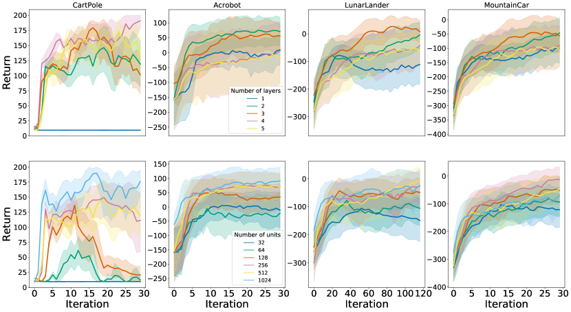
Figure 10: Evaluating DQN sensitivity to varying number of layers (top) and units per layer (bottom).

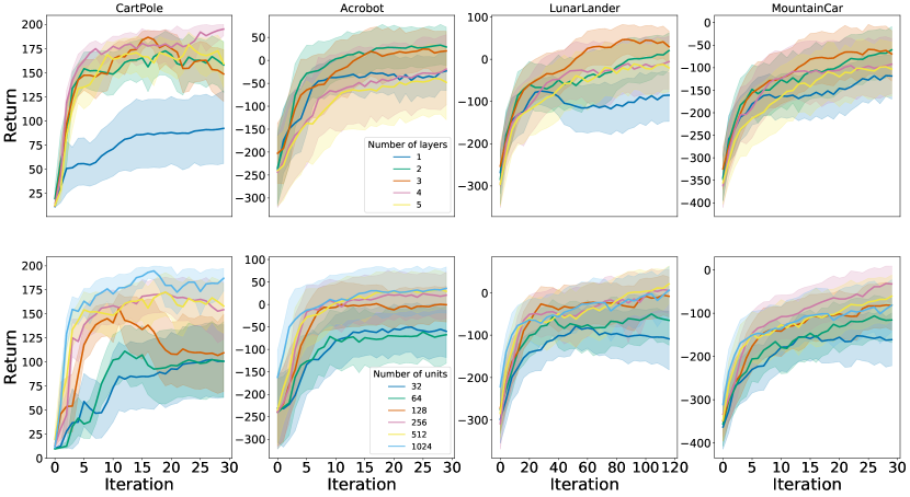
Figure 11: Evaluating Rainbow sensitivity to varying number of layers (top) and units per layer (bottom).

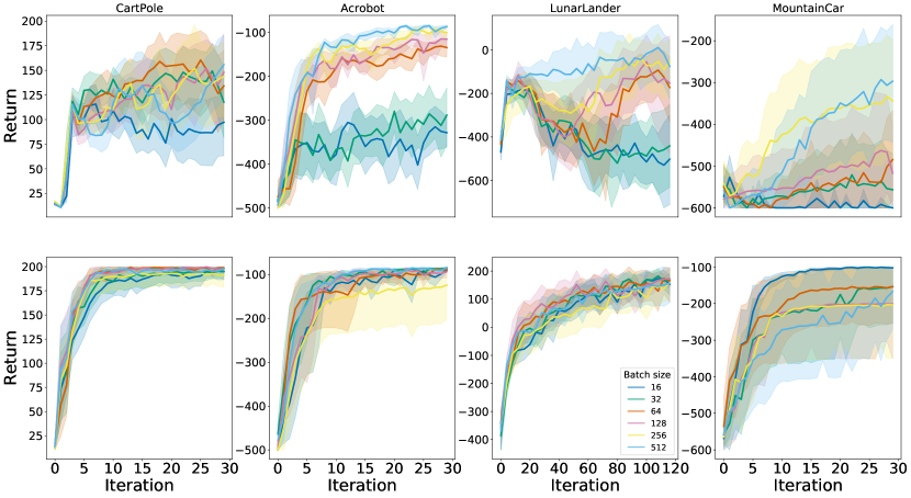
Figure 12: Evaluating DQN (top) and Rainbow (bottom) sensitivity to varying batch sizes. The default value used in the rest of the experiments is 128.

Appendix H Reevaluating the Huber loss, complete results

In this section we present complete results comparing the various combinations possible when using either Adam or RMSProp optimizers, and Huber or MSE losses.

H.1 Classic control and MinAtar results

We first evaluated the various combinations on all the classic control and MinAtar environments and found that Adam+MSE worked best. Full results displayed in Figure 13.

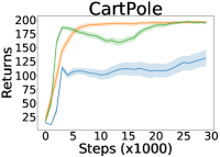
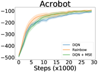
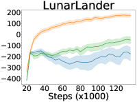
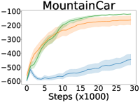
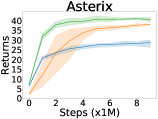
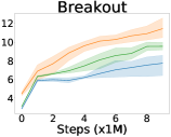
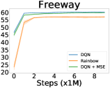
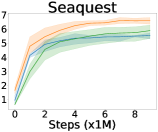
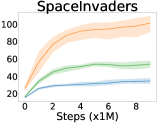
Figure 13: Evaluation of the use of the mean-squared error loss, instead of the Huber loss, in DQN.

H.2 Atari results

Given that the standard practice when training DQN is to use RMSPRop with the Huber loss, yet our results on the classic control and MinAtar environments suggest that MSE would work better, we performed a thorough comparison of the various combinations, which we present in this section.

We compare Adam vs RMSProp when both use the Huber loss (Figure 14) and MSE loss (Figure 15); we also compare the MSE vs Huber loss when using RMSProp (Figure 16) and using Adam (Figure 17). In Figure 18 we compare the various combinations using human normalized scores across all games, and we provide complete training curves for all games in Figure 19. As can be seen, the best results are obtained when using Adam and the MSE loss, in contrast to the standard practice of using RMSProp and the Huber loss.

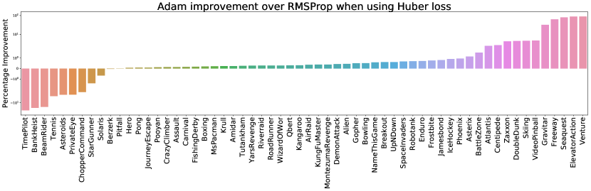
Figure 14: Comparing Adam vs RMSProp when both optimizers use the Huber loss.

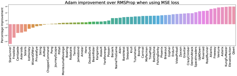
Figure 15: Comparing Adam vs RMSProp when both optimizers use the MSE loss.

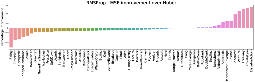
Figure 16: Comparing the MSE vs Huber loss when using the RMSProp optimizer.

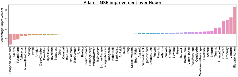
Figure 17: Comparing the MSE vs Huber loss when using the Adam optimizer.

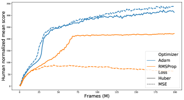
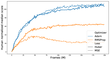
Figure 18: Comparison of the various optimizer-loss combinations with human normalized scores (mean left, median right). All results report the average of 5 independent runs.

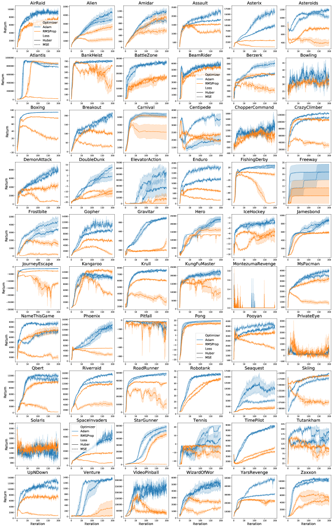
Figure 19: Comparison of using Adam (blue) versus RMSProp (orange) with Huber loss (solid) versus MSE loss (dashed) on all 60 Atari games. Each combination was run over 5 independent runs and the shaded areas represent 75% confidence intervals.

Appendix I Rainbow flavours, full results

In this section we present the complete results for all the environments when comparing DQN against the various Rainbow flavours (Figure 20).

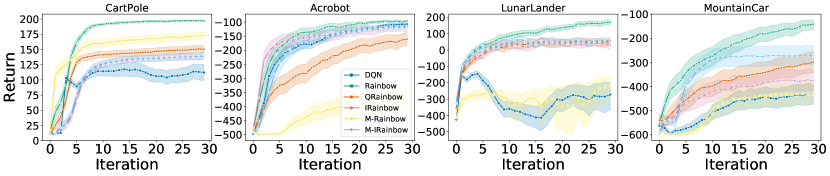
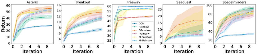
Figure 20: Comparing DQN against the various Rainbow flavours.

References

- Bacon et al. [2017] Pierre-Luc Bacon, Jean Harb, and Doina Precup. The option-critic architecture. In Proceedings of the Thirty-First AAAI Conference on Artificial Intelligence, AAAI’17, page 1726–1734, 2017.
- Bellemare et al. [2012] Marc G. Bellemare, Yavar Naddaf, Joel Veness, and Michael Bowling. The arcade learning environment: An evaluation platform for general agents. Journal of Artificial Intelligence Research, Vol. 47:253–279, 2012. cite arxiv:1207.4708.
- Bellemare et al. [2017] Marc G. Bellemare, Will Dabney, and Rémi Munos. A distributional perspective on reinforcement learning. In Proceedings of the 34th International Conference on Machine Learning - Volume 70, ICML’17, page 449–458, 2017.
- Brockman et al. [2016] Greg Brockman, Vicki Cheung, Ludwig Pettersson, Jonas Schneider, John Schulman, Jie Tang, and Wojciech Zaremba. Openai gym, 2016.
- Buckman et al. [2021] Jacob Buckman, Carles Gelada, and Marc G. Bellemare. The importance of pessimism in fixed-dataset policy optimization. In Proceedings of the Ninth International Conference on Learning Representations, ICLR’21, 2021.
- Castro [2020] Pablo Samuel Castro. Scalable methods for computing state similarity in deterministic Markov decision processes. In Proceedings of the AAAI Conference on Artificial Intelligence (AAAI), 2020.
- Castro et al. [2018] Pablo Samuel Castro, Subhodeep Moitra, Carles Gelada, Saurabh Kumar, and Marc G. Bellemare. Dopamine: A Research Framework for Deep Reinforcement Learning. 2018. URL http://arxiv.org/abs/1812.06110.
- Colas et al. [2018a] Cédric Colas, Olivier Sigaud, and Pierre-Yves Oudeyer. GEP-PG: Decoupling exploration and exploitation in deep reinforcement learning algorithms. In Jennifer Dy and Andreas Krause, editors, Proceedings of the 35th International Conference on Machine Learning, volume 80 of Proceedings of Machine Learning Research, pages 1039–1048. PMLR, 2018a.
- Colas et al. [2018b] Cédric Colas, Olivier Sigaud, and Pierre-Yves Oudeyer. How many random seeds? statistical power analysis in deep reinforcement learning experiments. CoRR, abs/1806.08295, 2018b.
- Dabney et al. [2018a] W. Dabney, M. Rowland, Marc G. Bellemare, and R. Munos. Distributional reinforcement learning with quantile regression. In AAAI, 2018a.
- Dabney et al. [2017] Will Dabney, Mark Rowland, Marc G. Bellemare, and Rémi Munos. Distributional reinforcement learning with quantile regression, 2017.
- Dabney et al. [2018b] Will Dabney, Georg Ostrovski, David Silver, and Remi Munos. Implicit quantile networks for distributional reinforcement learning. In Proceedings of the 35th International Conference on Machine Learning, volume 80 of Proceedings of Machine Learning Research, pages 1096–1105. PMLR, 2018b.
- Declan et al. [2020] Oller Declan, Glasmachers Tobias, and Cuccu Giuseppe. Analyzing reinforcement learning benchmarks with random weight guessing. Proceedigns of the International Conference on Autonomous Agents and Multiagent Systems, AAMAS 2020, pages 975–982, 2020.
- Fortunato et al. [2018] Meire Fortunato, Mohammad Gheshlaghi Azar, Bilal Piot, Jacob Menick, Ian Osband, Alexander Graves, Vlad Mnih, Remi Munos, Demis Hassabis, Olivier Pietquin, Charles Blundell, and Shane Legg. Noisy networks for exploration. In Proceedings of the International Conference on Representation Learning (ICLR 2018), Vancouver (Canada), 2018.
- Fujimoto et al. [2020] Scott Fujimoto, David Meger, and Doina Precup. An equivalence between loss functions and non-uniform sampling in experience replay. In Advances in Neural Information Processing Systems 33 (NeurIPS 2020), 2020.
- Ghiassian et al. [2020] Sina Ghiassian, Andrew Patterson, Shivam Garg, Dhawal Gupta, Adam White, and Martha White. Gradient temporal-difference learning with regularized corrections. In Hal Daumé III and Aarti Singh, editors, Proceedings of the 37th International Conference on Machine Learning, volume 119 of Proceedings of Machine Learning Research, pages 3524–3534. PMLR, 13–18 Jul 2020.
- Hasselt [2010] Hado V. Hasselt. Double q-learning. In Advances in Neural Information Processing Systems 23, pages 2613–2621. Curran Associates, Inc., 2010.
- Henderson et al. [2018] Peter Henderson, Riashat Islam, Philip Bachman, Joelle Pineau, Doina Precup, and David Meger. Deep reinforcement learning that matters. In Proceedings of the Thirthy-Second AAAI Conference On Artificial Intelligence (AAAI), 2018, 2018.
- Hessel et al. [2018] Matteo Hessel, Joseph Modayil, Hado van Hasselt, Tom Schaul, Georg Ostrovski, Will Dabney, Dan Horgan, Bilal Piot, Mohammad Azar, and David Silver. Rainbow: Combining Improvements in Deep Reinforcement learning. In Proceedings of the AAAI Conference on Artificial Intelligence, 2018.
- Hessel et al. [2019] Matteo Hessel, Hado van Hasselt, Joseph Modayil, and David Silver. On inductive biases in deep reinforcement learning. CoRR, abs/1907.02908, 2019.
- Huber [1964] Peter J. Huber. Robust Estimation of a Location Parameter. The Annals of Mathematical Statistics, 35(1):73 – 101, 1964. doi: 10.1214/aoms/1177703732. URL https://doi.org/10.1214/aoms/1177703732.
- Jordan et al. [2020] Scott Jordan, Yash Chandak, Daniel Cohen, Mengxue Zhang, and Philip Thomas. Evaluating the performance of reinforcement learning algorithms. In Hal Daumé III and Aarti Singh, editors, Proceedings of the 37th International Conference on Machine Learning, volume 119 of Proceedings of Machine Learning Research, pages 4962–4973. PMLR, 13–18 Jul 2020.
- Kingma and Ba [2015] Diederik P. Kingma and Jimmy Ba. Adam: A method for stochastic optimization. In Yoshua Bengio and Yann LeCun, editors, 3rd International Conference on Learning Representations, ICLR 2015, San Diego, CA, USA, May 7-9, 2015, Conference Track Proceedings, 2015. URL http://arxiv.org/abs/1412.6980.
- Lin [1992] Long-Ji Lin. Self-improving reactive agents based on reinforcement learning, planning and teaching. Mach. Learn., 8(3–4):293–321, May 1992.
- Lyle et al. [2019] Clare Lyle, Marc G. Bellemare, and Pablo Samuel Castro. A comparative analysis of expected and distributional reinforcement learning. In AAAI, 2019.
- Machado et al. [2018] Marlos C. Machado, Marc G. Bellemare, Erik Talvitie, Joel Veness, Matthew Hausknecht, and Michael Bowling. Revisiting the Arcade Learning Environment: Evaluation protocols and open problems for general agents. Journal of Artificial Intelligence Research, 2018.
- Mnih et al. [2015] Volodymyr Mnih, Koray Kavukcuoglu, David Silver, Andrei A. Rusu, Joel Veness, Marc G. Bellemare, Alex Graves, Martin Riedmiller, Andreas K. Fidjeland, Georg Ostrovski, Stig Petersen, Charles Beattie, Amir Sadik, Ioannis Antonoglou, Helen King, Dharshan Kumaran, Daan Wierstra, Shane Legg, and Demis Hassabis. Human-level control through deep reinforcement learning. Nature, 518(7540):529–533, February 2015.
- Nachum et al. [2019] Ofir Nachum, Yinlam Chow, Bo Dai, and Lihong Li. Dualdice: Behavior-agnostic estimation of discounted stationary distribution corrections. NeurIPS, 2019.
- Osband et al. [2020] Ian Osband, Yotam Doron, Matteo Hessel, John Aslanides, Eren Sezener, Andre Saraiva, Katrina McKinney, Tor Lattimore, Csaba Szepesvári, Satinder Singh, Benjamin Van Roy, Richard Sutton, David Silver, and Hado van Hasselt. Behaviour suite for reinforcement learning. In International Conference on Learning Representations, 2020. URL https://openreview.net/forum?id=rygf-kSYwH.
- Puterman [1994] Martin L. Puterman. Markov Decision Processes: Discrete Stochastic Dynamic Programming. John Wiley & Sons, Inc., New York, NY, USA, 1st edition, 1994. ISBN 0471619779.
- Schaul et al. [2016] Tom Schaul, John Quan, Ioannis Antonoglou, and David Silver. Prioritized experience replay. In Proceedings of ICLR, 2016, 2016.
- Sutton [1988] Richard S. Sutton. Learning to predict by the methods of temporal differences. Machine Learning, 3(1):9–44, August 1988.
- Tang et al. [2017] Haoran Tang, Rein Houthooft, Davis Foote, Adam Stooke, OpenAI Xi Chen, Yan Duan, John Schulman, Filip DeTurck, and Pieter Abbeel. #exploration: A study of count-based exploration for deep reinforcement learning. In I. Guyon, U. V. Luxburg, S. Bengio, H. Wallach, R. Fergus, S. Vishwanathan, and R. Garnett, editors, Advances in Neural Information Processing Systems, volume 30, pages 2753–2762. Curran Associates, Inc., 2017. URL https://proceedings.neurips.cc/paper/2017/file/3a20f62a0af1aa152670bab3c602feed-Paper.pdf.
- Tassa et al. [2020] Yuval Tassa, Saran Tunyasuvunakool, Alistair Muldal, Yotam Doron, Siqi Liu, Steven Bohez, Josh Merel, Tom Erez, Timothy Lillicrap, and Nicolas Heess. dm_control: Software and tasks for continuous control, 2020.
- Todorov et al. [2012] Emanuel Todorov, Tom Erez, and Yuval Tassa. Mujoco: A physics engine for model-based control. In IROS, pages 5026–5033. IEEE, 2012.
- van Hasselt et al. [2016] Hado van Hasselt, Arthur Guez, and David Silver. Deep reinforcement learning with double q-learning. In Proceedings of the Thirthieth AAAI Conference On Artificial Intelligence (AAAI), 2016, 2016. cite arxiv:1509.06461Comment: AAAI 2016.
- Vieillard et al. [2020] Nino Vieillard, Olivier Pietquin, and Matthieu Geist. Munchausen reinforcement learning, 2020.
- Wang et al. [2016] Ziyu Wang, Tom Schaul, Matteo Hessel, Hado Hasselt, Marc Lanctot, and Nando Freitas. Dueling network architectures for deep reinforcement learning. In Proceedings of the 33rd International Conference on Machine Learning, volume 48, pages 1995–2003, 2016.
- Young and Tian [2019] Kenny Young and Tian Tian. Minatar: An atari-inspired testbed for thorough and reproducible reinforcement learning experiments. arXiv preprint arXiv:1903.03176, 2019.