Cost Function Unrolling in Unsupervised Optical Flow

Abstract

Steepest descent algorithms, which are commonly used in deep learning, use the gradient as the descent direction, either as-is or after a direction shift using preconditioning. In many scenarios calculating the gradient is numerically hard due to complex or non-differentiable cost functions, specifically next to singular points. In this work we focus on the derivation of the Total Variation semi-norm commonly used in unsupervised cost functions. Specifically, we derive a differentiable proxy to the hard $L^{1}$ smoothness constraint in a novel iterative scheme which we refer to as Cost Unrolling. Producing more accurate gradients during training, our method enables finer predictions of a given DNN model through improved convergence, without modifying its architecture or increasing computational complexity. We demonstrate our method in the unsupervised optical flow task. Replacing the $L^{1}$ smoothness constraint with our unrolled cost during the training of a well known baseline, we report improved results on both MPI Sintel and KITTI 2015 unsupervised optical flow benchmarks. Particularly, we report EPE reduced by up to 15.82% on occluded pixels, where the smoothness constraint is dominant, enabling the detection of much sharper motion edges.

1 Introduction

The $L^{1}$ norm of the gradients of a given function, also known as Total Variation (TV) semi-norm, and more specifically its estimation, has been a significant field of study in robust statistics [11]. Even prior to the sweeping AI era, many approaches to Computer Vision problems, such as image restoration, denoising and registration [25, 26, 34], have used a TV regularizer, as it represents the prior distribution of pixel intensities of natural images [10]. Its main advantage is its robustness to small oscillations such as noise while preserving sharp discontinuities such as edges.

Historically, solving the TV problem has been a challenging task, mainly due to the non-differenetiabilty of the $L^{1}$ norm at zero. As a result, differentiable relaxations have been proposed, such as the Huber [12] and Charbonnier [7] loss functions. Further approaches involved iterative variational methods and have shown superior results in many tasks [3, 34, 25]. Introducing trainable Deep Neural Networks (DNNs) to Computer Vision has brought a significant performance boost, and specifically the commonly used auto-derivation frameworks [24, 15, 1] have provided quick and easy tools to solve complex functions. Indeed, these frameworks commonly bypass the $L^{1}$ non-differentiability either by a differentiable proxy or using its sub-gradients. We claim that non-differentiable cost functions should be dealt with greater care, as was done for many years before the deep learning era.

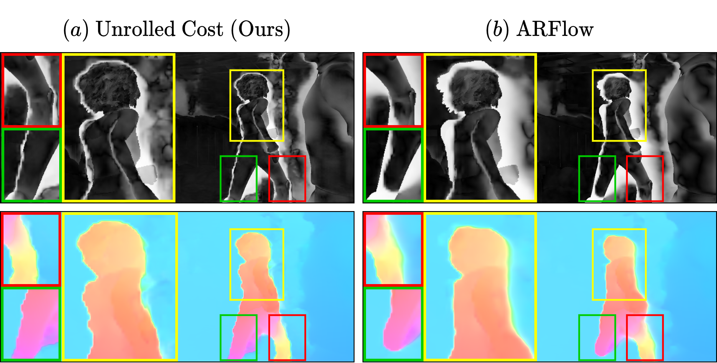
Figure 1: Sintel Final benchmark qualitative example. Introducing our method to the unsupervised optical flow domain, our unrolled cost function enables the detection of sharper motion boundaries through improved convergence, without modifying the model’s architecture or increasing complexity. Displayed are the predicted Sintel Final benchmark ’Market 1’ flows (bottom) and errors (top) of both our method and the ARFlow [18] baseline, with close-ups on specific regions. White regions feature measured high errors.

Proximal iterative methods for learning complex functions have shown superiority in many Image Processing, as well as Computer Vision tasks [33, 23, 35]. In these works, axiomatic optimization algorithms are unrolled and each iteration is mapped to a sub-network having its own learnable parameters. The resulting network architectures consist of task specific stacked modules which may be trained end-to-end in both supervised and unsupervised manners. Performance boost has been achieved either by increasing the number of stacked modules [33] or introducing intermediate modules [20, 32], both resulting in increased model complexity and size.

In this paper, we shift unrolling to the cost function, improving DNN model optimization while preserving its architecture as opposed to standard unrolling. Specifically, we present a novel pipeline we refer to as Cost Unrolling, in which we unroll the commonly used unsupervised cost function consisting of a data term and TV smoothness regularization, to obtain an iterative proxy. Following the well known Alternating Direction Method of Multiplies (ADMM) [3] algorithm, our initial optimization problem is iteratively decomposed into a set of sub-problems, each one featuring a differentiable cost function. Gradients computed using all sub-cost functions at each training step are shown to be more accurate in the regions where the gradients of the original cost function are hard to evaluate or undefined, improving convergence.

We demonstrate the effectiveness of our unrolled cost function in synthetic experiments, as well as the unsupervised optical flow domain. The lack of available labeled data has made unsupervised optical flow learning a significant field of interest. Used cost functions commonly consist of a measure for image consistency and TV smoothness regularization. The occluded pixels, pixels within a reference image with no correspondence at the target image, are masked out when measuring image consistency. As a result, occluded regions, which are highly correlated to motion boundaries, are mostly dominated by the gradients of the smoothness constraint.

Our unrolled cost function is introduced to the recently published unsupervised optical flow pipeline ARFlow [18]. Replacing their used TV smoothness constraint with our unrolled cost during all phases of training produces improved results on both MPI Sintel [4] and KITTI 2015 [22] unsupervised optical flow benchmarks. Particularly, we report EPE reduced by up to 15.82% on occluded pixels, where the smoothness constraint is dominant, allowing the detection of much sharper motion edges, as is highly visible in figures 1 and 5.

1.1 Contributions

We summarize our contributions as follows:

• Present the first unrolled cost function in deep learning for TV regularized problems.

• Demonstrate our proposed pipeline in the real-life unsupervised optical flow domain.

• Report improved results on unsupervised optical flow benchmarks, achieved without modifying model architecture or increasing complexity.

2 Related Work

Total Variation (TV) minimization has been a significant field of research in robust statistics [11]. It was introduced to Image Processing and Computer Vision tasks by [25] and showed superior performance over previous methods mainly due to its edge preserving property. However, solving TV regularized problems has shown to be non-trivial, mainly as the $L^{1}$ norm is non-differentiable at zero. Differentiable relaxations were proposed by [12, 7, 5], however iterative variational methods have proven more effective [26, 34, 3].

Introducing trainable DNN models to Computer Vision tasks has brought a significant performance boost. The lack of labeled data available for training has pushed many DNN algorithms towards unsupervised learning. Not surprisingly, the TV smoothness regularization can be found in the cost functions of many unsupervised works both past and recent. As DNN algorithms use gradient descent algorithms for optimization, the non-differentiability of the $L^{1}$ norm at zero has been commonly bypassed either by differentiable approximations [21] or by using its sub-gradients [17, 16, 20].

Algorithm unrolling is an iterative structured approach for learning complex functions, in which iterative operations derived from axiomatic algorithms determine the model architecture. A vast review of the topic is presented in [23]. Axiomatic algorithms, such as the Alternating Direction Method of Multipliers (ADMM) [3], Half Quadratic Splitting (HQS) [2] or Primal-Dual method [6], have inspired many deep algorithm unrolling frameworks. Indeed, ADMM-Net [29] introduced a DNN model for compressed sensing with architecture derived from ADMM, USRNet [35] learned Single Image Super-Resolution (SISR) using a deep framework inspired by HQS and [33] demonstrated an iterative structure derived from a Primal-Dual solver, aimed to refine the optical flow predicted by a FlowNet [8] model.

However, these frameworks feature closed form update steps derived from the learned objective function, which are mapped into task specific sub-networks trained in a supervised manner, increasing model size and complexity. As opposed to standard unrolling, we demonstrate improving the optimization of a given DNN model while preserving its architecture. We unroll the commonly used unsupervised cost function consisting of a data term and TV smoothness regularization, to obtain an iterative differentiable proxy which produces more accurate gradients during training (demonstrated in the experimentation section). While previous works designed dedicated unrolled learnable units, we present a pipeline that can be applied to any model architecture.

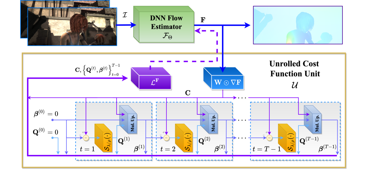
Figure 2: Unrolled cost block diagram for unsupervised optical flow. In each training iteration, given a flow prediction, its weighted spatial gradients $\mathbf{C}$ are computed. Once obtained, the Soft Thresholding and Multipliers Update operations are carried for update steps $t\in\{0,...,T-1\}$ to produce $\{\mathbf{Q}^{(t)},\boldsymbol{\beta}^{(t)}\}_{t=0}^{T-1}$, which are then used together with $\mathbf{C}$ to construct the unrolled loss function in (10). As our unrolled cost is computed only during training, our method does not affect inference.

Learning in iterations has shown to be very effective at both image registration and optical flow tasks. While FlowNet and FlowNet 2.0 [8, 13] were the first to learn optical flow, they were surpassed in both supervised and unsupervised settings, by the well known PWC-Net [28] which featured a course-to-fine iterative scheme. RAFT [30] introduced a fully iterative architecture which enabled a significant performance boost, as well as its expansion to the unsupervised settings [27]. Further approaches, such as [33, 32, 20], managed to improve the results of existing frameworks by adding intermediate modules and parameters for better flow refinement, which increase model size and complexity.

Here we demonstrate that unlike all other methods, improving the ability of a model to predict a finer flow can be achieved simply through improving the computed gradients during training.

3 Cost Function Unrolling

A general formulation of the cost function used for unsupervised learning consists of a data term, measuring the likelihood of a given prediction over the given data, as well as a prior term, constraining probable predictions. In this work we consider the TV regularized unsupervised cost function case and unroll it to obtain our novel smoothness regularizer. Denote by $\Theta$ the set of trainable parameters of a DNN model, its predicted output $\mathbf{F}$ and the set of unlabeled training data $\mathcal{I}$. The unsupervised TV regularized cost function takes the form:

$$\mathcal{L}(\mathcal{I},\Theta)=\mathbf{\Phi}\left(\mathbf{F},\mathcal{I}\right)+\lambda\|\nabla\mathbf{F}\|_{1}$$ (1)

where $\mathbf{\Phi(\cdot)}$ is a differentiable function measuring the likelihood of $\mathbf{F}$ over the training data $\mathcal{I}$, $\nabla\mathbf{F}$ are its spatial gradients, $\|\cdot\|_{1}$ is the $L^{1}$ norm and $\lambda$ is a hyperparameter controlling regularization.

3.1 Unrolling the Unsupervised Cost Function

Our goal is to minimize the objective function in (1). Following the ADMM [3] algorithm, we derive the iterative update steps minimizing (1), which are then used to construct our unrolled cost function. Let us examine the following optimization problem:

$$\hat{\mathbf{F}}=\arg\min_{\mathbf{F}}\left\{\mathbf{\Phi}\left(\mathbf{F},\mathcal{I}\right)+\lambda\|\nabla\mathbf{F}\|_{1}\right\}$$ (2)

We rewrite (2), introducing an auxiliary variable $\mathbf{Q}$:

$$\mathbf{\hat{F},\hat{Q}}= \arg\min_{\mathbf{F,Q}}\left\{\mathbf{\Phi}\left(\mathbf{F},\mathcal{I}\right)+\lambda\|\mathbf{Q}\|_{1}\right\}$$ (3)

$$\text{s.t.}\quad\mathbf{Q=\nabla F}$$

The augmented Lagrangian is then constructed as follows:

$$\mathcal{L}_{\rho}(\mathbf{F,Q},\boldsymbol{\alpha})=\mathbf{\Phi}\left(\mathbf{F},\mathcal{I}\right)+\lambda\|\mathbf{Q}\|_{1}$$ (4)

$$+\mathbf{\left<\boldsymbol{\alpha},Q-\nabla F\right>}_{2}+\frac{\rho}{2}\mathbf{\|Q-\nabla F\|}_{2}^{2}$$

where $\boldsymbol{\alpha}$ is the Lagrange Multipliers matrix and $\rho$ is a penalty parameter. Substituting $\boldsymbol{\beta}=\frac{\boldsymbol{\alpha}}{\rho}$ for simplicity, we iteratively optimize $\mathbf{\{F,Q,\boldsymbol{\beta}\}}$ through solving the sub-problems (5a), (5b) and update the multipliers (5c) in each iteration:

$$\hat{\mathbf{F}}= \min_{\mathbf{F}}\left\{\mathbf{\Phi}\left(\mathbf{F},\mathcal{I}\right)+\frac{\rho}{2}\mathbf{\|Q-\nabla F+\boldsymbol{\beta}\|}_{2}^{2}\right\}$$ (5a)

$$\hat{\mathbf{Q}}= \min_{\mathbf{Q}}\left\{\mathbf{\lambda\|Q\|_{1}}+\frac{\rho}{2}\mathbf{\|Q-\nabla F+\boldsymbol{\beta}\|}_{2}^{2}\right\}$$ (5b)

$$\boldsymbol{\beta}\leftarrow \boldsymbol{\beta}+\eta\mathbf{\left(Q-\nabla F\right)}$$ (5c)

with $\eta$ an update rate. The solutions to the problems in (5a) and (5b) are referred to as the ADMM update steps for $\mathbf{F}$ and $\mathbf{Q}$, respectively.

3.2 Solving the Sub-Optimization Problems

Solutions to the sub-optimization problems in equations (5a) and (5b) are now discussed. While the problem in equation (5b) has a closed form solution, deriving a closed form solution for the problem in (5a) is not trivial, as $\mathbf{\Phi}$ can be any function. Substituting $\mathbf{C=\nabla F}$, (5b) reduces to:

$$\min_{\mathbf{Q}}\left\{\mathbf{\lambda\|Q\|}_{1}+\frac{\rho}{2}\mathbf{\|Q-C+\boldsymbol{\beta}\|}_{2}^{2}\right\}$$ (6)

$$=\min_{\mathbf{Q}}\left\{\lambda\sum_{i}|Q_{i}|+\frac{\rho}{2}\sum_{i}|Q_{i}-C_{i}+\beta_{i}|^{2}\right\}$$

$$=\sum_{i}\min_{Q_{i}}\left\{\lambda|Q_{i}|+\frac{\rho}{2}|Q_{i}-C_{i}+\beta_{i}|^{2}\right\}$$

where $A_{i}$ are the matrix elements of $\mathbf{A}$, i.e. the problem is separable and we may solve independently for each matrix element. The objective in (6) is convex and its solution is the well known Soft Thresholding operator $\hat{Q}_{i}=\mathcal{S}_{\lambda/\rho}\left(C_{i}-\beta_{i}\right)$, defined:

$$\mathcal{S}_{\lambda/\rho}(x)=\begin{cases}0,&|x|<\lambda/\rho\\ x-\frac{\lambda}{\rho}\text{sign}(x),&|x|\geq\lambda/\rho\end{cases}$$ (7)

The Soft Thresholding operator performs shrinkage of the input signal, thus it promotes sparse solutions.

We now consider the sub-problem in equation (5a). Using the same substitution as in (6), we wish to optimize:

$$\min_{\mathbf{F}}\left\{\mathbf{\Phi}\left(\mathbf{F},\mathcal{I}\right)+\frac{\rho}{2}\mathbf{\|Q-C+\boldsymbol{\beta}\|}_{2}^{2}\right\}$$ (8)

Deriving a closed form solution is not trivial, as we wish to optimize for any $\mathbf{\Phi(\cdot)}$. However, note that the problem in (8) consists of the same data term as in (2) with the TV smoothness regularizer replaced by a softer, differentiable constraint. Re-substituting into eq. (8), the constraint takes the form:

$$\frac{\rho}{2}\|\mathcal{S}_{\lambda/\rho}\left(\nabla\mathbf{F}-\boldsymbol{\beta}\right)-\left(\nabla\mathbf{F}-\boldsymbol{\beta}\right)\|_{2}^{2}$$ (9)

Recall that minimizing the TV of a function promotes sparse output gradients. In fact, (9) yields a differentiable alternative for TV minimization, as it suggests minimizing the $L^{2}$ distance between the true and sparsified output gradients in each ADMM iteration. This realization stands in the core of our approach.

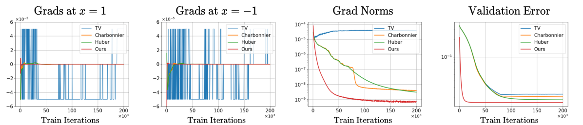
Figure 3: PC signal prediction - training. We train a simple model to predict a full PC 1D function given a small set of sampled points and TV regularization, using our unrolled cost, as well as TV cost function and common TV relaxation methods. From right to left: displayed are the validation errors and gradient norms, recorded during training, as well as gradients measured at $x=-1$ and $x=1$, respectively. As can be seen, our unrolled cost not only achieves the best results, but it also converges the fastest and the smoothest.

3.3 Unrolled Cost Function

Our unrolled cost function is inspired by the ADMM update steps given in equations (5a),(5b),(5c). However, instead of explicitly refining $\mathbf{F}$ in each iteration as in standard unrolling, we aim to solve the iterative sub-problems given in (5a) simultaneously, updating $\mathbf{Q},\boldsymbol{\beta}$ alone given a fixed model prediction $\mathbf{F}$.

Our proposed unrolled cost function takes the form:

$$\mathcal{L}^{\mathbf{F}}(\mathcal{I},\Theta)= \mathbf{\Phi}\left(\mathbf{F},\mathcal{I}\right)$$ (10)

$$+ \frac{\rho}{2}\frac{1}{T}\sum_{t=0}^{T-1}\|\mathbf{Q}^{(t)}+\boldsymbol{\beta}^{(t)}-\mathbf{C}\|_{2}^{2}$$

where:

$$\mathbf{Q}^{(t)} =\mathcal{S}_{\lambda/\rho}\left(\mathbf{\nabla F}-\boldsymbol{\beta}^{(t-1)}\right)$$ (11a)

$$\boldsymbol{\beta}^{(t)} =\boldsymbol{\beta}^{(t-1)}+\eta\mathbf{\left(Q^{(t)}-\nabla F\right)}$$ (11b)

$ֿC =∇F$and$T$isahyperparameterstatingthenumberofupdatestepscarried.Thus,ateachtrainingiteration,givenamodelprediction$F$,itsspatialgradients$C$arecalculatedandusedtoiterativelycompute${Q^(t),β^(t)}_t=0^T-1$.Allupdatetermsarethenaccumulatedtoconstructthesmoothnessconstraintin(\ref{eq:loss_f}),whichisusedformodeltraining.Ablockdiagramfortheunsupervisedopticalflowsetting(describedinsection\ref{sec:of})isshowninfigure\ref{fig:unrol_arch}.Beingfullydifferentiable,specificallyarounditsoptimum,ourunrolledsmoothnessconstraintproducesmoreaccurategradients,convergesmoreefficientlyandimprovesperformance,asisshownintheexperimentationsection.$

4 Experimentation

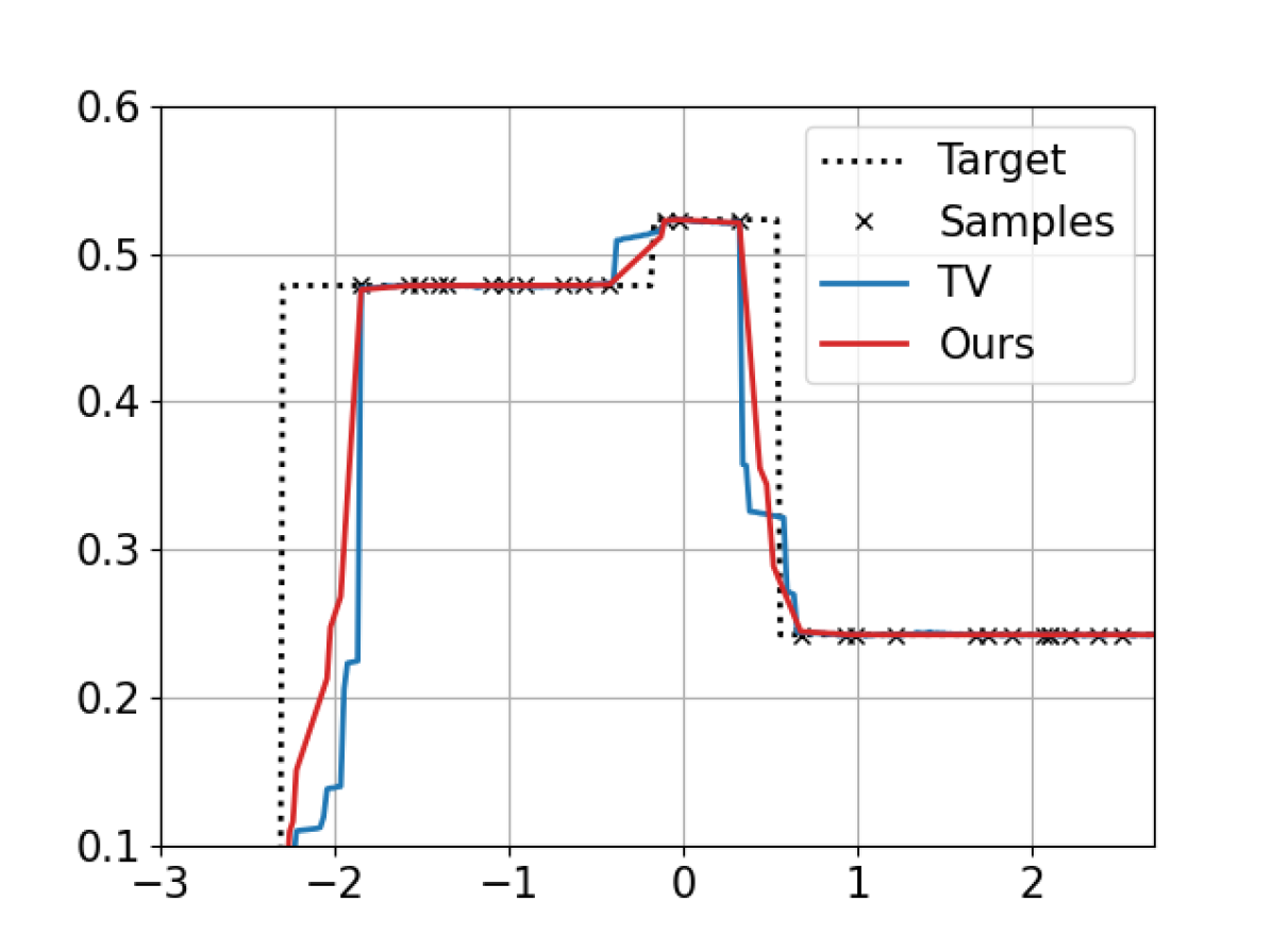
Figure 4: PC signal prediction - target vs. predicted signals. Displayed are the generated target signal, its samples and signals predicted by models trained using either standard TV regularization or our unrolled cost function. As can be seen, our unrolled cost overcomes the staircasing effect, promoting a solution which is both smooth and edge preserving.

We demonstrate the effectiveness of our method through conducting experiments in two domains: piece-wise constant (PC) signal prediction (section 4.1) and unsupervised optical flow (section 4.2).

We further compare our unrolled cost to standard TV smoothness regularization, as well as $L^{1}$ relaxation baselines: Huber [12] and Charbonnier [7] loss functions. The Huber regularizer over a prediction $\mathbf{x}$ is defined as $\mathcal{R}_{H}(\mathbf{x};k)=\sum_{i}r_{H}(x_{i};k)$, where:

$$r_{H}(x_{i};k)=\begin{cases}\frac{1}{2}x_{i}^{2},&|x_{i}|<k\\ k|x_{i}|-\frac{1}{2}k^{2}&|x_{i}|\geq k\end{cases}$$ (12)

and $x_{i}$ are the elements of $\mathbf{x}$. It aims to take advantage of the $L^{1}$ norm robustness to outliers, but suggests better convergence replacing $L^{1}$ by $L^{2}$ for points near its optimum. The Charbonnier regularizer is defined as $\mathcal{R}_{C}(\mathbf{x})=\sum_{i}r_{C}(x_{i})$, where:

$$r_{C}(x_{i})=\sqrt{x_{i}^{2}+\epsilon^{2}}$$ (13)

We show that our iterative approach is superior to these $L^{1}$ relaxations, achieving improved results and faster convergence.

4.1 PC Signal Prediction

We randomly generate a 1D Piece-wise Constant (PC) signal $y(x),x\in[a,b]$ and sample it uniformly to generate our training data $\{(x_{i},y_{i})\}_{i=0}^{N-1}$ where $y_{i}=y(x_{i})$. We over-fit a small NN model, consisting of 4 FC layers to predict the full signal given its samples, using GD iterations (see figure 4). We define our data term:

Method	Grad Norm	Error
Standard TV	$3.86\times 10^{-5}$	$2.29\times 10^{-2}$
Charbonnier [7]	$4.00\times 10^{-9}$	$2.07\times 10^{-2}$
Huber [12]	$3.11\times 10^{-9}$	$1.84\times 10^{-2}$
Unrolled Cost	$\mathbf{6.38\times 10^{-10}}$	$\mathbf{1.65\times 10^{-2}}$

Table 1: PC signal prediction - measured results. Presented are the measured data losses and prediction errors of models trained using our unrolled cost, standard TV regularization and TV relaxations. Training using our unrolled cost decreases TV prediction error by 28.2%.

$$\mathbf{\Phi}\left(\mathbf{f},\mathcal{I}\right)=\frac{1}{N}\sum_{i=0}^{N-1}\left(f_{i}-y_{i}\right)^{2}$$ (14)

where $\{f_{i}\}_{i=0}^{N-1}$ are the corresponding samples of the predicted output. We train our model using our unrolled cost and compare to standard TV, Huber [12] and Charbonnier [7] baselines, measuring the prediction error as the mean absolute difference between target and predicted signals. We perform independent hyperparameter optimization prior to comparing both methods. We present here results of one scenario, further results as well as implementation details are available in the supplementary material.

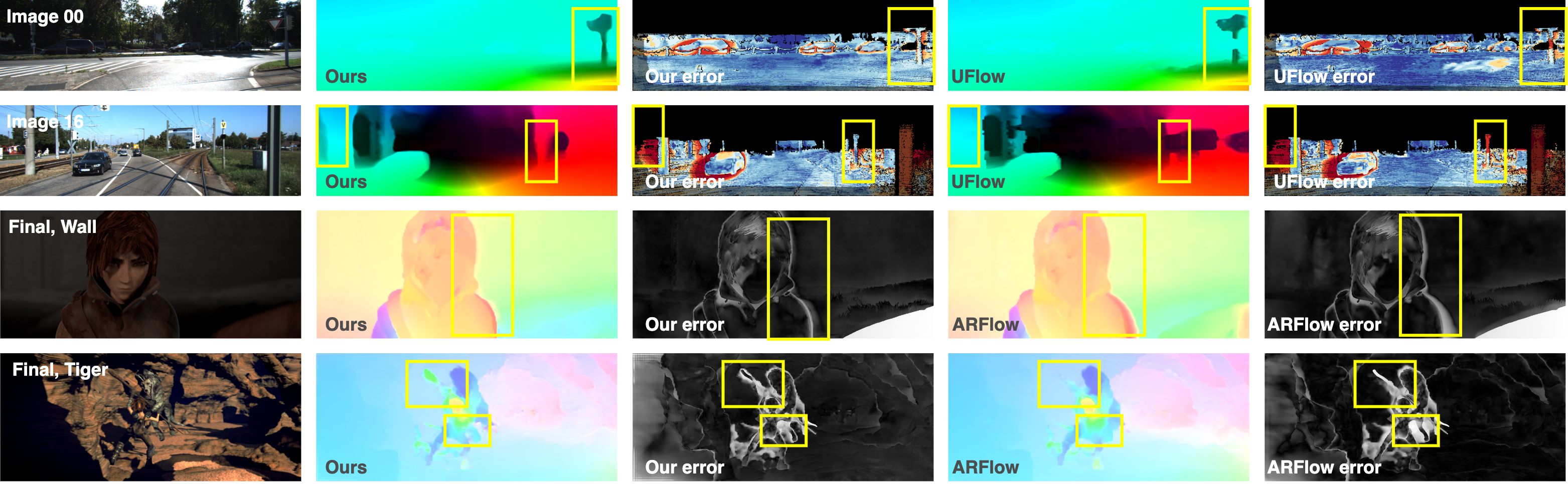
Figure 5: Qualitative benchmark results. We compare qualitative flow benchmark results of ours, the ARFlow [18] and UFlow [16] baselines. Both ARFlow and UFlow are methods adopting a PWC-Net [28] based backbone, reporting the best results on the MPI Sintel [4] and KITTI 2015 [22] benchmarks, respectively. We find adapting our unrolled cost to a PWC-Net based backbone outperforms both baselines, particularly at the motion boundaries.

4.1.1 Prediction Error

We compare the signals predicted by our models. Prediction errors are given in table 1. The target, its samples and predicted signals are shown in figure 4. We find that training using our unrolled cost decreases TV prediction error by 28.2%, enabling a smoother but edge preserving solution (see fig. 4).

4.1.2 Convergence

We study the convergence of all methods. Figure 3 displays prediction errors and gradient norms recorded during training, as well as gradients recorded at selected points (other points may be viewed in the supplementary material). We find our method not only achieves better results, but it also converges nearly two times faster than TV. Further inspecting the gradients generated during training reveals that gradients of the TV suffer from severe oscillations as a result of its non-differentiabilty at zero. These oscillations cause the measured gradient norms to increase rather than decrease, suggesting an unstable optimum. While $L^{1}$ relaxation baselines feature improved results and convergence compared to TV, our method achieves the best results and converges the fastest with its gradients smoothly decreasing to zero.

4.2 Unsupervised Optical Flow

We next test our proposed unrolled cost on the real-world unsupervised optical flow problem. We introduce our unrolled cost to the recently published ARFlow [18] baseline, rigorously following their proposed training scheme and model architecture, yet replacing their used TV regularization with our method. Optical flow is defined as a mapping $\mathbf{F}:\mathbb{R}^{2}\mapsto\mathbb{R}^{2}$, which aligns pixels given a pair of images $I_{1},I_{2}$. In the unsupervised optical flow setting, our data term takes the form:

$$\mathbf{\Phi}\left(\mathbf{F},\mathcal{I}\right)=\mathbf{\Phi}\left(I_{1},\hat{I}_{2}^{\mathbf{F}}\right)$$ (15)

i.e. $\mathbf{\Phi}$ is a differetiable photometric loss, measuring the consistency of a reference image and a target image warped using $\mathbf{F}$. In order to remain consistent with the ARFlow baseline, we use masked TV regularization, substituting $\mathbf{C=W\odot\nabla F}$ into equation (10), where $\mathbf{W}$ is a deterministic importance matrix, aiming to increase the penalty on the boundaries, defined:

$$\mathbf{W} =\exp\left\{-\alpha|\nabla I_{1}|\right\}$$ (16)

$$=\exp\left\{-\alpha\left[\left|\frac{\partial I_{1}}{\partial x}\right|,\left|\frac{\partial I_{1}}{\partial y}\right|\right]\right\}$$

and $\alpha$ is an hyperparameter controlling the masking operation. A block diagram of our method for the unsupervised optical flow setting is shown in figure 2.

Method	Sintel Clean			Sintel Final			KITTI 2015
	Occ.	Noc.	All	Occ.	Noc.	All	Occ.	Noc.	All
Standard TV	8.77	1.27	2.29	9.97	2.19	3.22	6.51	2.16	2.91
Charbonnier [7]	8.96	1.31	2.34	9.98	2.20	3.22	6.23	2.13	2.89
Huber [12]	8.80	1.26	2.27	10.10	2.22	3.27	6.60	2.11	2.93
Unrolled Cost (Ours)	7.91	1.28	2.17	9.16	2.13	3.06	5.48	2.14	2.82

Table 2: Unrolled cost vs. TV relaxations - unsupervised optical flow. Our method outperforms all tested $L^{1}$ relaxation baselines. Furthermore, our method decreases the TV EPE averaged over the occluded regions, which are highly affected by the smoothness constraint, by up to 15.82%, enabling the detection of sharper motion boundaries without any modification to the model architecture or complexity.

4.2.1 Model

Following the ARFlow [18] baseline, we use a PWC-Net based model consisting of a 7 level multi-resolution pyramid. The model is trained end-to-end in a fully unsupervised manner. The photometric loss term is evaluated on non-occluded regions only, thus occluded regions are optimized using only the smoothness regularization. The training scheme consists of both pre-training and finetuning. During finetuning, self-supervision is acquired through appearance, spatial and occlusion pseudo-random deformations, as elaborated next. Further implementation details are available in the supplementary material.

Self-supervision from Augmentations

As carried by ARFlow, self-supervision from pseudo-random augmentations is applied during finetunine. Image and corresponding flow augmentations, $\mathcal{T}^{\text{img}}:I_{k}\mapsto\tilde{I}_{k}$ and $\mathcal{T}^{\text{flow}}:\mathbf{F\mapsto\tilde{F}}$ respectively, perform a combination of appearance, spatial and occlusion pseudo-random deformations. An initial flow estimate $\mathbf{F}_{1}$ is computed given a pair of images $I_{1},I_{2}$. The image pair then undergoes an image augmentation $\mathcal{T}^{\text{img}}$ resulting in a deformed pair of images $\tilde{I}_{1},\tilde{I}_{2}$. A second flow estimate $\mathbf{F}_{2}$ is generated next over the deformed images $\tilde{I}_{1},\tilde{I}_{2}$. Finally, we acquire self-supervision obtaining $\mathbf{\tilde{F}}_{1}$ through applying the flow augmentation $\mathcal{T}^{\text{flow}}$ over $\mathbf{F}_{1}$ and measuring the error $\mathbf{F}_{2}-\mathbf{\tilde{F}}_{1}$.

4.2.2 Datasets

We evaluate our method on well-known optical flow benchmarks: the synthetic MPI Sintel [4] and real-world autonomous driving KITTI 2015 [22].

We follow the ARFlow [18] training scheme. For the MPI Sintel benchmark, we first pretrain our model on the raw Sintel movie. $12,466$ image pairs are extracted and split according to scene shots. We then finetune our model on the official training set, consisting of $1,041$ image pairs, each rendered with $2$ levels of difficulty. For the KITTI 2015 benchmark, we first pretrain our model on the KITTI raw dataset [9], which consists of real road scenes captured by a car-mounted stereo camera rig. We then use the KITTI 2015 multi-view extension for finetuning. We exclude frames related to validation from our training set, i.e. use only frames below 9 or above 12 in each scene. Further details regarding the train-test data splitting used in our experiments are given in the supplementary.

4.2.3 Flow in Occluded Regions

Occluded pixels, i.e. pixels with no correspondence, are highly correlated with motion boundaries. Although crucial to many CV applications, performance on the occluded regions minorly affects the errors averaged over full images. We test our method particularly on occluded pixels as they are mostly affected by the gradients of the smoothness constraint during training. As official benchmark results don’t report errors in occluded regions, we validate our models on the available official training data using train-test splitting (see supplementary). Measured validation AEPE rates of our unrolled cost, as well as the standard TV, Huber [12] and Charbonnier [7] baselines are given in table 2. Our method outperforms all tested baselines. As expected, modifying the smoothness regularizer has little effect on the performance in the non-occluded regions (Noc.). However, measuring the performance on the occluded regions, our method reduces TV EPE rates by up to 15.82% enabling the detection of sharper motion boundaries with no added complexity. Qualitative flow visualizations are displayed in figures 1 and 5.

Method	Sintel Clean		Sintel Final		KITTI 2015
	Train	Test	Train	Test	Train	Test (F1)
CoT-AMFlow ⋆ [32]	-	3.96	-	5.14	-	10.34%
STFlow ⋆ [31]	(2.91)	6.12	(3.59)	6.63	3.56	13.83%
UPFlow ⋆ [20]	(2.33)	4.68	(2.67)	5.32	2.45	9.38%
SMURF ⋆ [27]	(1.71)	3.15	(2.58)	4.18	(2.00)	6.83%
DDFlow [19]	(2.92)	6.18	(3.98)	7.40	5.72	14.29%
UFlow-train [16]	(2.50)	5.21	(3.39)	6.50	(2.71)	11.13%
SimFlow [14]	(2.86)	5.92	(3.57)	6.92	5.19	13.38%
ARFlow [18]	(2.79)	4.78	(3.73)	5.89	2.85	11.80%
UnrolledCost (Ours)	(2.75)	4.69	(3.61)	5.80	2.87	10.81%

Table 3: MPI Sintel & KITTI 2015 official unsupervised optical flow benchmark results. We report AEPE and F1 rates for recently published unsupervised methods on both the MPI Sintel [4] and KITTI 2015 [22] optical flow benchmarks. Methods featuring a different backbone are marked with $\star$. Brackets ”()” indicate results of models trained using their validation set. Best methods in each category are in bold. Missing results are marked as ”-”. By adapting our unrolled cost to the ARFlow [18] baseline we not only achieve improved results, but also report the best results for a PWC-Net based backbone on both benchmarks at the time of submission. Moreover, we find our method highly effective on the motion boundaries, as shown in the qualitative results (figures 1,5).

4.2.4 Comparison with State of the Art

We compare our trained model with recently published unsupervised methods on the MPI Sintel and KITTI 2015 optical flow benchmarks in table 3. The used measures are the Average End-Point-Error (AEPE) and F1 score, measuring outliers percentage (error $>$ 3px). Our method managed to improve the reported results of the ARFlow [18] baseline on both MPI Sintel and the KITTI 2015 unsupervised optical flow benchmarks, particularly at the motion boundaries, as is highly visible in figures 5 and 1. Moreover, our method reports the best results using a PWC-Net based backbone on dual images at the time of submission.

4.2.5 Number of Cost Function Update Steps

$\#$ Update Steps	Sintel Clean	Sintel Final
$T=1$	2.43	3.25
$T=2$	2.35	3.19
$\mathbf{T=4}$	2.35	3.16

Table 4: Number of cost function update steps. Finetuning using several $T$ values, we find that increasing the number of update steps brings a performance boost.

Method	Memory	Runtime
Standard TV	4.326Gi	51ms
Unrolled Cost (Ours)	4.285Gi	51ms

Table 5: Computational complexity. Our method consumes slightly less memory during training and preserves runtime, hence replacing TV regularization with our unrolled cost enables improved results with no added complexity.

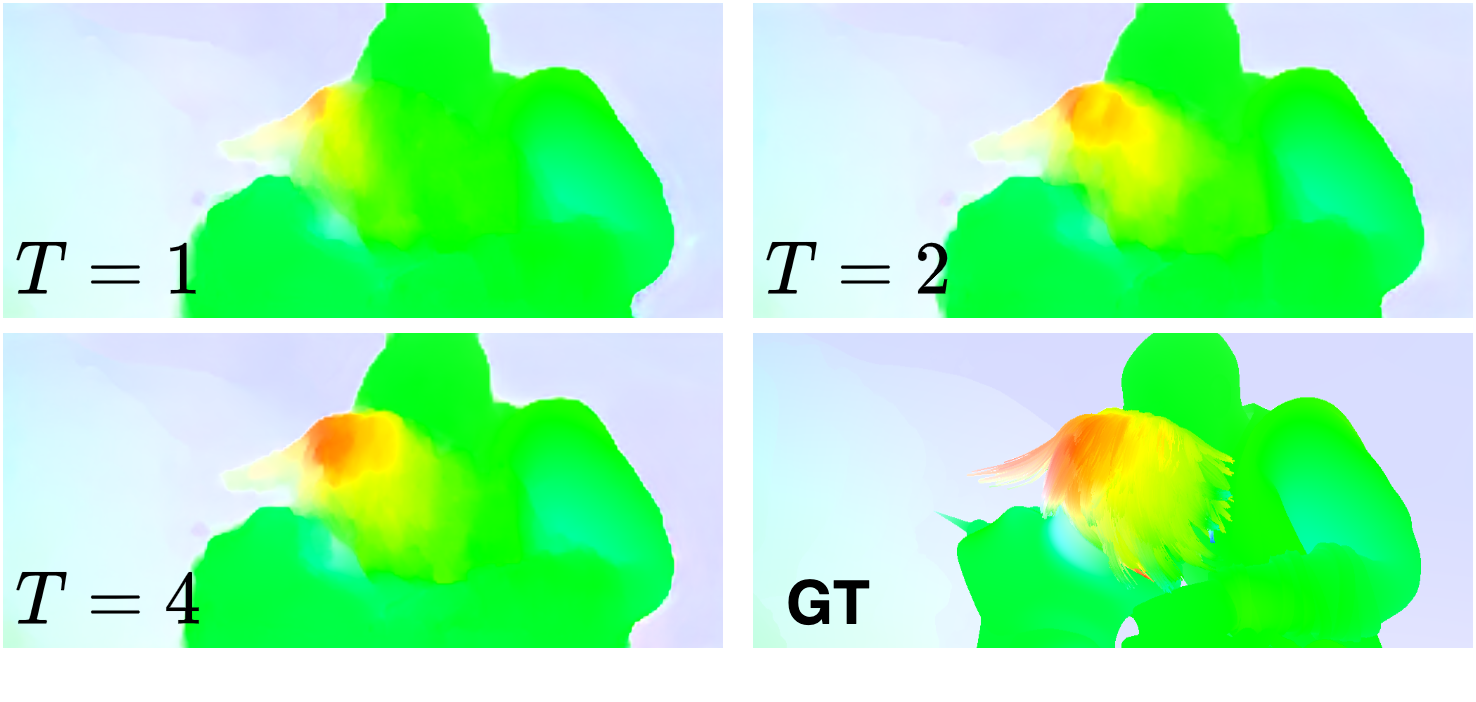
Figure 6: Qualitative example - number of update steps. We find increasing the number of update steps improves the ability of our model to capture finer flow details.

We study the effective number of cost function update steps $T$ required for training. We use a model which has been pretrained on the MPI Sintel raw movie and set various $T$ values during finetuning. Several $T$ values are compared in table 4 and a qualitative example is shown in figure 6. We find that increasing $T$ brings a performance boost, enabling our flow estimator to capture finer motion details. However, further investigating the convergence of the cost function update steps during training shows that convergence is achieved at $T=2$ making the gain for setting setting $T>2$ relatively small. Additional study regarding update steps convergence is given in the supplementary material. Substituting $T=2$ in eq. (10), we conclude that our effective TV regularization proxy consists of the $L^{2}$ norm of the spatial gradients, as well as one update step.

4.2.6 Computational Complexity

As our method deals with model training alone, it does not affects inference. We compare both memory consumption and training time of our method to the ARFlow [18] baseline in table 5. All measurements are carried using a batch size of 4 image pairs and an image size of $384\times 832$ over an RTX2080 GPU. Our method does not increase model size, as no learned parameters are added. Furthermore, as we set our unrolled cost unit to operate at flow original resolution, which is 1/4 image resolution, our method consumes slightly less memory and preserves training time.

5 Conclusions

We introduced the concept of Cost Unrolling, shifting algorithm unrolling to the cost function, while preserving model architecture. Our method enables improved training of a TV regularized model as a result of more accurate gradients, thanks to its differentiability around its optimum, preserving complexity. We have demonstrated the effectiveness of our method in a synthetic signal prediction problem as well as real-world unsupervised optical flow. Our unrolled cost achieved superior results in all tested scenarios. We believe that the proposed framework can be applied on top of other model architectures for boosting their results next to non-differentiable optimum solutions.

References

- [1] Martín Abadi, Ashish Agarwal, Paul Barham, Eugene Brevdo, Zhifeng Chen, Craig Citro, Greg S. Corrado, Andy Davis, Jeffrey Dean, Matthieu Devin, Sanjay Ghemawat, Ian Goodfellow, Andrew Harp, Geoffrey Irving, Michael Isard, Yangqing Jia, Rafal Jozefowicz, Lukasz Kaiser, Manjunath Kudlur, Josh Levenberg, Dandelion Mané, Rajat Monga, Sherry Moore, Derek Murray, Chris Olah, Mike Schuster, Jonathon Shlens, Benoit Steiner, Ilya Sutskever, Kunal Talwar, Paul Tucker, Vincent Vanhoucke, Vijay Vasudevan, Fernanda Viégas, Oriol Vinyals, Pete Warden, Martin Wattenberg, Martin Wicke, Yuan Yu, and Xiaoqiang Zheng. TensorFlow: Large-scale machine learning on heterogeneous systems, 2015. Software available from tensorflow.org.
- [2] M. V. Afonso, J. M. Bioucas-Dias, and M. A. T. Figueiredo. Fast image recovery using variable splitting and constrained optimization. IEEE Transactions on Image Processing, 19(9):2345–2356, 2010.
- [3] Stephen Boyd, Neal Parikh, Eric Chu, Borja Peleato, and Jonathan Eckstein. Distributed optimization and statistical learning via the alternating direction method of multipliers. Found. Trends Mach. Learn., 3(1):1–122, Jan. 2011.
- [4] D. J. Butler, J. Wulff, G. B. Stanley, and M. J. Black. A naturalistic open source movie for optical flow evaluation. In A. Fitzgibbon et al. (Eds.), editor, European Conf. on Computer Vision (ECCV), Part IV, LNCS 7577, pages 611–625. Springer-Verlag, Oct. 2012.
- [5] A. Chambolle and P. Lions. Image recovery via total variation minimization and related problems. Numerische Mathematik, 76:167–188, 1997.
- [6] Antonin Chambolle and Thomas Pock. A first-order primal-dual algorithm for convex problems with applications to imaging. Journal of mathematical imaging and vision, 40(1):120–145, 2011.
- [7] Pierre Charbonnier, Laure Blanc-Féraud, Gilles Aubert, and Michel Barlaud. Deterministic edge-preserving regularization in computed imaging. IEEE Transactions on image processing, 6(2):298–311, 1997.
- [8] Alexey Dosovitskiy, Philipp Fischer, Eddy Ilg, Philip Hausser, Caner Hazirbas, Vladimir Golkov, Patrick Van Der Smagt, Daniel Cremers, and Thomas Brox. Flownet: Learning optical flow with convolutional networks. In Proceedings of the IEEE international conference on computer vision, pages 2758–2766, 2015.
- [9] Andreas Geiger, Philip Lenz, Christoph Stiller, and Raquel Urtasun. Vision meets robotics: The kitti dataset. International Journal of Robotics Research (IJRR), 2013.
- [10] Jinggang Huang and D. Mumford. Statistics of natural images and models. In Proceedings. 1999 IEEE Computer Society Conference on Computer Vision and Pattern Recognition (Cat. No PR00149), volume 1, pages 541–547 Vol. 1, 1999.
- [11] P.J. Huber, J. Wiley, and W. InterScience. Robust statistics. Wiley New York, 1981.
- [12] Peter J Huber. Robust estimation of a location parameter: Annals mathematics statistics, 35. 1964.
- [13] Eddy Ilg, Nikolaus Mayer, Tonmoy Saikia, Margret Keuper, Alexey Dosovitskiy, and Thomas Brox. Flownet 2.0: Evolution of optical flow estimation with deep networks. In Proceedings of the IEEE conference on computer vision and pattern recognition, pages 2462–2470, 2017.
- [14] Woobin Im, Tae-Kyun Kim, and Sung-Eui Yoon. Unsupervised learning of optical flow with deep feature similarity. In European Conference on Computer Vision, pages 172–188. Springer, 2020.
- [15] Yangqing Jia, Evan Shelhamer, Jeff Donahue, Sergey Karayev, Jonathan Long, Ross Girshick, Sergio Guadarrama, and Trevor Darrell. Caffe: Convolutional architecture for fast feature embedding. arXiv preprint arXiv:1408.5093, 2014.
- [16] Rico Jonschkowski, Austin Stone, Jonathan T Barron, Ariel Gordon, Kurt Konolige, and Anelia Angelova. What matters in unsupervised optical flow. arXiv preprint arXiv:2006.04902, 2020.
- [17] Wonjik Kim, Asako Kanezaki, and Masayuki Tanaka. Unsupervised learning of image segmentation based on differentiable feature clustering. IEEE Transactions on Image Processing, 29:8055–8068, 2020.
- [18] Liang Liu, Jiangning Zhang, Ruifei He, Yong Liu, Yabiao Wang, Ying Tai, Donghao Luo, Chengjie Wang, Jilin Li, and Feiyue Huang. Learning by analogy: Reliable supervision from transformations for unsupervised optical flow estimation. In IEEE Conference on Computer Vision and Pattern Recognition(CVPR), 2020.
- [19] Pengpeng Liu, Irwin King, Michael R Lyu, and Jia Xu. Ddflow: Learning optical flow with unlabeled data distillation. In Proceedings of the AAAI Conference on Artificial Intelligence, volume 33, pages 8770–8777, 2019.
- [20] Kunming Luo, Chuan Wang, Shuaicheng Liu, Haoqiang Fan, Jue Wang, and Jian Sun. Upflow: Upsampling pyramid for unsupervised optical flow learning. In Proceedings of the IEEE/CVF Conference on Computer Vision and Pattern Recognition, pages 1045–1054, 2021.
- [21] Simon Meister, Junhwa Hur, and Stefan Roth. Unflow: Unsupervised learning of optical flow with a bidirectional census loss. arXiv preprint arXiv:1711.07837, 2017.
- [22] Moritz Menze and Andreas Geiger. Object scene flow for autonomous vehicles. In Conference on Computer Vision and Pattern Recognition (CVPR), 2015.
- [23] Vishal Monga, Yuelong Li, and Yonina C Eldar. Algorithm unrolling: Interpretable, efficient deep learning for signal and image processing. arXiv preprint arXiv:1912.10557, 2019.
- [24] Adam Paszke, Sam Gross, Francisco Massa, Adam Lerer, James Bradbury, Gregory Chanan, Trevor Killeen, Zeming Lin, Natalia Gimelshein, Luca Antiga, Alban Desmaison, Andreas Kopf, Edward Yang, Zachary DeVito, Martin Raison, Alykhan Tejani, Sasank Chilamkurthy, Benoit Steiner, Lu Fang, Junjie Bai, and Soumith Chintala. Pytorch: An imperative style, high-performance deep learning library. In H. Wallach, H. Larochelle, A. Beygelzimer, F. d'Alché-Buc, E. Fox, and R. Garnett, editors, Advances in Neural Information Processing Systems 32, pages 8024–8035. Curran Associates, Inc., 2019.
- [25] Leonid I. Rudin, Stanley Osher, and Emad Fatemi. Nonlinear total variation based noise removal algorithms. Physica D: Nonlinear Phenomena, 60(1):259–268, 1992.
- [26] Joseph Savage and Ke Chen. An improved and accelerated non-linear multigrid method for total-variation denoising. International Journal of Computer Mathematics, 82(8):1001–1015, 2005.
- [27] Austin Stone, Daniel Maurer, Alper Ayvaci, Anelia Angelova, and Rico Jonschkowski. Smurf: Self-teaching multi-frame unsupervised raft with full-image warping. In Proceedings of the IEEE/CVF Conference on Computer Vision and Pattern Recognition, pages 3887–3896, 2021.
- [28] Deqing Sun, Xiaodong Yang, Ming-Yu Liu, and Jan Kautz. PWC-Net: CNNs for optical flow using pyramid, warping, and cost volume. 2018.
- [29] Jian Sun, Huibin Li, Zongben Xu, et al. Deep admm-net for compressive sensing mri. In Advances in neural information processing systems, pages 10–18, 2016.
- [30] Zachary Teed and Jia Deng. Raft: Recurrent all-pairs field transforms for optical flow. arXiv preprint arXiv:2003.12039, 2020.
- [31] Long Tian, Zhigang Tu, Dejun Zhang, Jun Liu, Baoxin Li, and Junsong Yuan. Unsupervised learning of optical flow with cnn-based non-local filtering. IEEE Transactions on Image Processing, 29:8429–8442, 2020.
- [32] Hengli Wang, Rui Fan, and Ming Liu. Cot-amflow: Adaptive modulation network with co-teaching strategy for unsupervised optical flow estimation. arXiv preprint arXiv:2011.02156, 2020.
- [33] Shenlong Wang, Sanja Fidler, and Raquel Urtasun. Proximal deep structured models. In Proceedings of the 30th International Conference on Neural Information Processing Systems, NIPS’16, page 865–873, Red Hook, NY, USA, 2016. Curran Associates Inc.
- [34] Christopher Zach, Thomas Pock, and Horst Bischof. A duality based approach for realtime tv-l 1 optical flow. In Joint pattern recognition symposium, pages 214–223. Springer, 2007.
- [35] Kai Zhang, Luc Van Gool, and Radu Timofte. Deep unfolding network for image super-resolution. In Proceedings of the IEEE/CVF Conference on Computer Vision and Pattern Recognition, pages 3217–3226, 2020.