Testing for Uniqueness of Estimators

Abstract

Uniqueness of the population value of an estimated descriptor is a standard assumption in asymptotic theory. However, m-estimation problems often allow for local minima of the sample estimating function, which may stem from multiple global minima of the underlying population estimating function. In the present article, we provide tools to systematically determine for a given sample whether the underlying population estimating function may have multiple global minima. To achieve this goal, we develop asymptotic theory for non-unique minimizers and introduce asymptotic tests using the bootstrap. We discuss three applications of our tests to data, each of which presents a typical scenario in which non-uniqueness of descriptors may occur. These model scenarios are the mean on a non-euclidean space, non-linear regression and Gaussian mixture clustering.

1 Introduction

Asymptotic theory is a cornerstone of statistics and an important underpinning for the use of asymptotic distribution quantiles in hypothesis tests. For this reason, asymptotic theory has been generalized to a variety of different settings. Here we focus on m-estimators, which are a fairly broad class of estimators. Most of the motivation, examples and simulations consider the Fréchet mean on manifolds but our results are applicable to a variety of different scenarios as illustrated by our data applications. To be as general as possible, we develop asymptotic theory for non-Euclidean data and descriptor spaces. Asymptotic theory for such settings has been developed among others by Hendriks and Landsman (1998); Bhattacharya and Patrangenaru (2005); Huckemann (2011); Bhattacharya and Lin (2017). Notably, Eltzner and Huckemann (2019) even extends asymptotic theory to probability measures featuring a lower asymptotic rate than $n^{-1/2}$, a phenomenon termed “smeariness”.

In the literature on the asymptotics of m-estimators on non-Euclidean data spaces, it is usually assumed that the population value of the descriptor is unique. However, straight forward examples like two uniform modes centered at antipodal points of a circle or a uniform distribution on the equator of a sphere show that the population mean may not be unique. On the other hand, real data always consists only of finitely many values, therefore one might ask whether the sample descriptor is unique under more general conditions. Arnaudon and Miclo (2014) showed that for a sample from a continuously distributed random variable the sample Fréchet mean is almost surely unique.

Given this result, one may be tempted to rely on the sample mean as a meaningful data descriptor, since it is unique under general conditions. Furthermore, it is conceivable that the result can be generalized to a broad class of m-estimators. However, it is not clear, whether a sample with a unique descriptor may have been drawn from a population with non-unique descriptor. If this is the case, the full descriptor set of the population is not adequately reflected by the sample descriptor and conclusions from the sample descriptor may be invalid.

Here, we approach this problem and devise a hypothesis test for non-uniqueness of the population descriptor. The hypothesis test proceeds in three steps. First, for a sample of size $n$ determine the sample descriptor $\widehat{\mu}_{n}$ and generate $B$ n-out-of-n bootstrap samples and calculate the bootstrap descriptors $\mu_{n,n}^{*,i}$. Second, determine whether there are multiple clusters in the set of bootstrap descriptors $\{\mu_{n,n}^{*,i}\}_{i}$ and count the number $k$ of bootstrap descriptors, which are in another cluster than $\widehat{\mu}_{n}$. Last, if $2k/B<\alpha$ reject the null hypothesis of a non-unique descriptor and conclude at level $\alpha$ that the descriptor $\mu$ is unique. If the test does not reject, one has to take possible non-uniqueness of the descriptor into account.

The null hypothesis of the test we propose states that the population descriptor is not unique. This is done for two reasons, one conceptually and one practical. First, in this setup, the alternative is the safe case, in which standard tools can be applied, while caution is advisable if the test does not reject the null. Thus, the error of first kind, assuming the situation is safe when it is not, appears the right error to bound. Second, the distribution of the test statistic under the null must be known in order to be able to give quantiles, while the distribution of the test statistic under the alternative is useful to determine the power of the test. In cases like ours, where the distribution of the test statistic under the alternative is unknown, the power of the test can be explored numerically.

To show the asymptotic size of the test, it is necessary to consider asymptotics of the minimum value of the estimating function. However, none of the quantities that appear in the asymptotic theory need to be calculated for the test we propose. If the m-estimating function is squared distance, the descriptor being estimated is the Fréchet mean while the minimum of the estimating function is the Fréchet variance. A Central Limit Theorem (CLT) for the Fréchet variance on general metric spaces was given by Dubey and Müller (2019). This article will extend this CLT to m-estimation loss, which is the minimal value of the cost function, not the value of the minimizing descriptor, and show that even if a descriptor is smeary for some measure, i.e. its asymptotic rate is slower than $n^{-1/2}$, the asymptotic rate of the loss remains $n^{-1/2}$.

To see how the hypothesis test is connected to asymptotic theory of the loss, we outline the test here. The null hypothesis of our test is that there are a number $m>1$ of global minimizers $\mu^{i}$. Let $\widehat{V}_{n}^{i}$ denote the sample loss in the neighborhood of any $\mu^{i}$ and let $W^{ij}$ be the CLT variance such that $\sqrt{n}(\widehat{V}_{n}^{i}-\widehat{V}_{n}^{j})\to N(0,W^{ij})$. For any $i$ consider the index sets $I_{i}:=\{1,\dots,i-1,i+1,\dots,m\}$. Then the type I error $\zeta_{n}$ is given by the probability that the sample loss $\widehat{V}_{n}^{i}$ in the neighborhood of any $\mu^{i}$ is smaller by at least the normal quantile $\frac{\sqrt{W^{ij}}}{\sqrt{n}}q\left(\frac{\alpha}{2}\right)$ than all other $\widehat{V}_{n}^{j}$, where $q$ is the standard normal quantile function,

$$\zeta_{n}(\alpha):=\sum_{i=1}^{m}\mathbb{P}\left(\forall j\in I_{i}:\,\frac{\sqrt{n}}{\sqrt{W^{ij}}q\left(\frac{\alpha}{2}\right)}\left(\widehat{V}_{n}^{i}-\widehat{V}_{n}^{j}\right)\leq 1\right)\,.$$

Next we take n-out-of-n bootstrap samples and calculate bootstrap sample losses $V_{n,n}^{*,i}$ in the neighborhoods of the $\mu^{i}$. We define probabilities of bootstrap losses under the condition that $\widehat{V}_{n}^{i}-\widehat{V}_{n}^{j}\approx\frac{\sqrt{W^{ij}}}{\sqrt{n}}q\left(\frac{\alpha}{2}\right)$ for all $j$,

$$\xi_{n}(\alpha):=\lim_{\varepsilon\to 0}\mathbb{P}\left(\exists j\in I_{i}:\,V_{n,n}^{*,i}-V_{n,n}^{*,j}>0\,\middle|\,\forall j\in I_{i}:\,\frac{\sqrt{n}}{\sqrt{W^{ij}}q\left(\frac{\alpha}{2}\right)}\left(\widehat{V}_{n}^{i}-\widehat{V}_{n}^{j}\right)\in\left[1,1+\varepsilon\right]\right)\,.$$

Thus, $\xi_{n}$ is the probability that despite the fact that $\widehat{V}_{n}^{i}-\widehat{V}_{n}^{j}=\frac{\sqrt{W^{ij}}}{\sqrt{n}}q\left(\frac{\alpha}{2}\right)$ for all $j$, which is the boundary of the error region of first kind, the bootstrap loss $V_{n,n}^{*,i}$ is not the smallest, but there is some $V_{n,n}^{*,j}<V_{n,n}^{*,i}$. This means that the bootstrap minimizer $\mu_{n,n}^{*}$ will not be close to the sample minimizer $\widehat{\mu}_{n}=\widehat{\mu}_{n}^{i}$ but to the local sample minimizer $\widehat{\mu}_{n}^{j}$. In Theorem 3.21 it is shown that

$$\lim_{n\to\infty}2\xi_{n}(\alpha)\geq\alpha\geq\lim_{n\to\infty}\zeta_{n}(\alpha)$$

which means that we can achieve an asymptotically conservative test to level $\alpha$ in the following way: draw $B$ n-out-of-n bootstrap samples and count the number $k$ of bootstrap descriptors which are “far away” from the sample estimator $\widehat{\mu}_{n}$. If $2k/B<\alpha$, the test rejects and we can conclude that the descriptor is unique to the chosen level. Otherwise, the possibility that the mean is not unique cannot be rejected.

In order to determine which bootstrap descriptors are far away from $\widehat{\mu}_{n}$, we note that the set of sample descriptors of a population with a finite number of population descriptors $\mu^{i}$ will consist of a set of clusters around the $\mu^{i}$. The same will be true for bootstrap resamples from a sample so we determine whether there are clusters of bootstrap descriptors except the cluster containing $\widehat{\mu}_{n}$ and count the number of bootstrap descriptors in those other clusters. In order to determine whether there are separate clusters, we use a simple multiscale test, based on the test by Dümbgen and Walther (2008) for unimodality of the set of bootstrapped descriptors.

In all of the following, we call the minimum values of the population and sample Fréchet function the population and sample loss, respectively. In the case of the estimating function being the square distance, the loss is also known as the variance. However, to avoid confusion with the trace of the CLT-covariance, which is in the general case an unrelated quantity, we refrain from this term in the following.

We present extensive simulations as well as three data examples to show the wide range of application scenarios of our test. The first data set concerns the mean on a circle and is therefore very close to the motivating ideas presented above. The second application is to non-linear least-squares regression, formulated as an m-estimation problem. Such “curve fit” estimators are very common in the natural sciences and are therefore highly relevant. We find that, although the parameter space looks innocuous, curve fits are found to be non-unique in some cases. The third application concerns a Gaussian mixture which is used for clustering. This method and related centroid clustering methods are very commonly used and the question which number of clusters should be assumed to describe a data set is a well known subject of discussion. If one assumes the point of view that an unambiguous cluster result is essential, our test for non-uniqueness can be used as a model selection tool.

2 Loss Asymptotics on a Metric Space

In this section we revisit the central limit theorem for the loss, which plays a crucial role for our considerations. Especially, we will show that even when an estimator exhibits a lower asymptotic rate than $n^{-1/2}$, see e.g. Eltzner and Huckemann (2019), the asymptotic rate for the loss will remain $n^{-1/2}$ under fairly generic circumstances.

First, we introduce some basic notions, which will be necessary for the following. In all of the following let $Q$ be a topological space called the data space and $\mathcal{P}$ a separable topological space with continuous metric function $d$ called the parameter space. $\Omega$ is a probability space as usual. Let $\rho:\mathcal{P}\times Q\to\mathbb{R}$ a continuous function, $X:\Omega\to Q$ a $Q$-valued random variable and $X_{1},\dots,X_{n}\operatorname{\stackrel{{\scriptstyle i.i.d.}}{{\sim}}}X$ a random sample. Define Fréchet functions and descriptors for samples and populations

$$F(p) =\mathbb{E}[\rho(p,X)] F_{n}(\omega,p) =\frac{1}{n}\sum_{j=1}^{n}\limits\rho(p,X_{j}(\omega))$$ (1)

$$\ell =\inf_{p\in\mathcal{P}}\limits F(p) \ell_{n}(\omega) =\inf_{p\in\mathcal{P}}\limits F_{n}(\omega,p)$$ (2)

$$E =\left\{p\in\mathcal{P}:F(p)=\ell\right\} E_{n}(\omega) =\left\{p\in\mathcal{P}:F_{n}(\omega,p)=\ell_{n}(\omega)\right\}\,.$$ (3)

The elements of $E_{n}$, if it is non-empty, are commonly called m-estimators. The term “m-estimator” has been widely used in the field of robust statistics. In the field of Statistics on non-Euclidean spaces the term generalized Fréchet means has been introduced by Huckemann (2011) for m-estimators where the elements of $\mathcal{P}$ have an interpretation as geometrical objects, for example geodesics of $Q$. In the present article, we are not specifically concerned with robust m-estimators nor with geometric objects, so we use the term “m-estimator” in its general meaning.

Before continuing the exposition, we fix some notation.

Notation 2.1.

1. Denote “almost surely for $\omega\in\Omega$” as $\forall_{0}\omega\in\Omega$.

2. For a point $p\in\mathcal{P}$ and $\varepsilon>0$ let $B_{\varepsilon}(p)=\{p^{\prime}\in\mathcal{P}:d(p,p^{\prime})<\varepsilon\}$.

To define the asymptotics of the estimator $E_{n}$, it is first necessary to make sure that it is consistent, i. e. it converges to $E$ for large $n$. We will use a rather general formulation of consistency, introduced by Bhattacharya and Patrangenaru (2003) and based on earlier work by Ziezold (1977). Consistency has been derived by Bhattacharya and Patrangenaru (2003); Huckemann (2011) under a few technical conditions on $\rho$ as well as $\mathcal{P}$ satisfying separability and the cluster points of the sample Fréchet mean sets satisfying the Heine Borel property. In the present article we do not expand on this subject. We will simply require $E_{n}$ to be consistent in all of the following.

Assumption 2.2 (Bhattacharya-Patrangenaru strong consistency (BPSC)).

The estimator $E_{n}$ is Bhattacharya-Patrangenaru strongly consistent (BPSC), i.e. it satisfies

$$\forall\varepsilon>0\quad\forall_{0}\omega\in\Omega\quad\exists n>0\quad\forall k\geq n\quad\forall\widehat{\mu}_{k}\in E_{k}(\omega)\quad\exists\mu\in E:\quad d(\widehat{\mu}_{k},\mu)\leq\varepsilon$$

The proofs of BPSC given by (Bhattacharya and Patrangenaru, 2003, Theorem 2.3) and (Huckemann, 2011, Theorem A.4) do not assume that $E$ contains exactly one element, but that $E\neq\emptyset$. Therefore, the existing theory is readily applicable in our setting and we will not reproduce it here. The assumption of BPSC is fundamental to all arguments presented here and it is unlikely that it can be relaxed without requiring significant restrictions in return. For example, requiring only weak consistency in probability undermines Assumptions 3.3 and 3.17 below unless one restricts to bounded parameter spaces.

We will approach the case that the population descriptor is not unique but we will assume throughout this article that the population descriptor set consists of a finite number of points.

Assumption 2.3.

The set of population descriptors comprises $m$ points $E=\{\mu^{1},\dots,\mu^{m}\}\subset\mathcal{P}$ and we define $\delta>0$ such that $B_{\delta}(\mu^{j})\cap B_{\delta}(\mu^{k})=\emptyset$ holds for any two points in $E$.

This assumption excludes cases, where the population descriptor set contains is a submanifold of descriptor space. This can happen for example due to symmetry in the system leading to minima sets given by orbits of symmetry transformations. One simple example is the set of Fréchet means on a sphere with a point mass on the north pole and a point mass on the south pole, which is a circle of constant latitude. A generalization to such cases requires a different approach and is beyond the scope of the article.

In the following, we will briefly consider the general case that $\mathcal{P}$ is simply a metric space, not necessarily a manifold. The setting we use is very similar to the one used by Dubey and Müller (2019). However, for general m-estimator loss, we need the following additional assumption that the function $\rho$ exhibit some regularity beyond what is needed for strong consistency.

Assumption 2.4 (Almost Surely Locally Lipschitz).

Assume $\delta>0$ from Assumption 2.3 and that for every $\mu^{i}\in E$, there is a measurable function $\dot{\rho}^{i}:Q\to\mathbb{R}$ satisfying $\mathbb{E}[\dot{\rho}^{i}(X)^{2}]<\infty$ and a metric $d_{i}$ of $\mathcal{P}$, such that the following Lipschitz condition

$$|\rho(p_{1},X)-\rho(p_{2},X)|\leq\dot{\rho}^{i}(X)d_{i}(p_{1},p_{2})\quad\mathrm{a.s.}$$

holds for all $p_{1},p_{2}\in B_{\delta}(\mu^{i})$.

To understand the importance of this local Lipschitz condition, it is necessary to introduce some empirical process theory. In all of the following let $\mathcal{F}$ denote some class of functions from the data space $Q$ to $\mathbb{R}$.

Definition 2.5.

For a class of functions $\mathcal{F}$ from $Q$ to $\mathbb{R}$, an envelope function $F:Q\to\mathbb{R}$ is any function, such that for any $f\in\mathcal{F}$ and $q\in Q$, $|f(q)|\leq F(q)$.

The most important notion for the following is the notion of the bracketing entropy of a function class.

Definition 2.6.

For a class of functions $\mathcal{F}$ from $Q$ to $\mathbb{R}$, a norm $\|\,\|$ on $\mathcal{F}$ and $\varepsilon>0$, consider two functions $f_{1},f_{2}\in\mathcal{F}$ such that $\|f_{1}-f_{2}\|<\varepsilon$ and call

$$[f_{1},f_{2}](\varepsilon,\mathcal{F},\|\,\|):=\left\{f\in\mathcal{F}\,:\,\forall_{0}q\in Q\quad f_{1}(q)\leq f(q)\leq f_{2}(q)\right\}$$

an $\varepsilon$ bracket. Then the bracketing number $N_{[\,]}(\varepsilon,\mathcal{F},\|\,\|)$ is defined as the minimal number of $\varepsilon$ brackets needed such that their union is $\mathcal{F}$. If $\mathcal{F}$ has an envelope function $F$, the bracketing entropy is defined as

$$J_{[\,]}(\eta,\mathcal{F},\|\,\|):=\int_{0}^{\eta}\limits\sqrt{1+\log N_{[\,]}(\varepsilon\|F\|,\mathcal{F},\|\,\|)}\,d\varepsilon$$

The bracketing entropy for a function class is difficult to determine. However, there is a similar concept for general metric spaces, namely the covering entropy, which is usually much simpler to determine.

Definition 2.7.

For a totally bounded metric space $(\mathcal{P},d)$ and a size $\varepsilon$ the covering number $N(\varepsilon,\mathcal{P},d)$ is defined as the minimal number of $\varepsilon$ balls needed to cover $\mathcal{P}$. The covering entropy is defined as

$$J(\eta,\mathcal{P},d):=\int_{0}^{\eta}\limits\sqrt{1+\log N(\varepsilon,\mathcal{P},d)}\,d\varepsilon$$

The local Lipschitz condition 2.4 connects the bracketing number of a function class indexed by a totally bounded metric space to the covering number of this metric space. Consider the function classes $\mathcal{F}_{i}:=\Big{\{}\rho^{i}(p,\cdot)-\rho^{i}(\mu^{i},\cdot),p\in B_{\delta}(\mu^{i})\Big{\}}$, then the connection is as follows.

Theorem 2.8 (van der Vaart and Wellner (1996), Theorem 2.7.11).

Under assumption 2.4, we have for any norm $\|\,\|$ on $\mathcal{F}_{i}$

$$N_{[\,]}(2\varepsilon\|\dot{\rho}^{i}\|,\mathcal{F}_{i},\|\,\|)\leq N(\varepsilon,B_{\delta}(\mu^{i}),d_{i})\,.$$

For the next theorem we introduce the empirical process and two relevant norms.

Definition 2.9.

Let $Q$ be the data space and $P=\mathbb{P}\circ X^{-1}$ the distribution measure in $Q$ corresponding to the random variable $X$.

• For an i.i.d. sample $\{X_{1},\dots,X_{n}\}$ from $P$ let $\mathbb{P}_{n}:=\frac{1}{n}\sum_{j=1}^{n}\limits\delta_{X_{j}}$ be the empirical measure.

• For any measurable function $f:Q\to\mathbb{R}$ let $\mathbb{G}_{n}(f):=\sqrt{n}\big{(}\mathbb{P}_{n}f-Pf\big{)}$ be the empirical process.

• For any measurable function $f:Q\to\mathbb{R}$ let $\|f\|_{P,r}:=\left(\int|f|^{r}dP\right)^{\frac{1}{r}}$ be the $L_{r}(P)$ norm.
  For any class $\mathcal{F}$ of measurable functions let $\|\mathbb{G}_{n}\|_{\mathcal{F}}:=\sup_{f\in\mathcal{F}}\limits|\mathbb{G}_{n}(f)|$.

Theorem 2.10 (van der Vaart and Wellner (1996), Theorem 2.14.2).

For any class $\mathcal{F}$ of measurable functions with measurable envelope function $F$,

$$\mathbb{E}\left[\|\mathbb{G}_{n}\|_{\mathcal{F}}\right]\lesssim J_{[\,]}(1,\mathcal{F},L_{2}(P))\|F\|_{P,2}$$

Assumption 2.11 (Entropy bound).

For the classes $\mathcal{F}_{i}$ with envelope functions $2\delta\dot{\rho}^{i}$ the following entropy bound holds

$$\lim_{\delta\to 0}\limits\delta\int_{0}^{1}\limits\sqrt{1+\log N(\varepsilon\delta,B_{\delta}(\mu^{i}),d_{i})}\,d\varepsilon=0\,.$$

This entropy bound is fairly general as discussed in Dubey and Müller (2019). The proof of Theorem 3.5 shows that it holds in the finite dimensional manifold setting discussed below. Now, we have introduced all the tools necessary to extend the result of Dubey and Müller (2019) to general m-estimators. The results will be split into two parts as in Dubey and Müller (2019) in order to more clearly highlight the different steps

Proposition 2.12 (Preparation for the CLT).

Under Assumptions 2.2, 2.3, 2.4 and 2.11 we have, for a measurable selection $\widehat{\mu}_{n}^{i}\in\left\{x\in B_{\delta}(\mu^{i}):F_{n}(x)=\inf_{y\in B_{\delta}(\mu^{i})}\limits F_{n}(y)\right\}$

$$\sqrt{n}\big{(}F_{n}(\widehat{\mu}_{n}^{i})-F(\mu^{i})\big{)} =\sqrt{n}\big{(}F_{n}(\mu^{i})-F(\mu^{i})\big{)}+o_{P}(1)\,.$$

Proof.

We follow the strategy laid out in Dubey and Müller (2019) Proposition 3.

$$\mathbb{P}\left[\sqrt{n}|F_{n}(\widehat{\mu}_{n}^{i})-F_{n}(\mu^{i})|>\varepsilon\right]=\mathbb{P}\left[\sqrt{n}\left(F_{n}(\mu^{i})-F_{n}(\widehat{\nu}_{n}^{i})\right)>\varepsilon\right]$$

$$\leq \mathbb{P}\left[\sqrt{n}\left(F_{n}(\mu^{i})-F_{n}(\widehat{\mu}_{n}^{i})-\left(F(\mu^{i})-F(\widehat{\mu}_{n}^{i})\right)\right)>\varepsilon\right]$$

$$= \mathbb{P}\left[\sqrt{n}\left|F_{n}(\widehat{\mu}_{n}^{i})-F(\widehat{\mu}_{n}^{i})-\left(F_{n}(\mu^{i})-F(\mu^{i})\right)\right|>\varepsilon\right]$$

$$\leq \mathbb{P}\left[\sup_{|x^{i}|\leq\delta}\limits\sqrt{n}\left|F_{n}(x^{i})-F(x^{i})-\left(F_{n}(\mu^{i})-F(\mu^{i})\right)\right|>\varepsilon\right]+\mathbb{P}[|\widehat{\mu}_{n}^{i}|\geq\delta]$$

Now, we can apply the Markov inequality, and Assumption 2.2 to get

$$\mathbb{P}\left[\sqrt{n}|F_{n}(\widehat{\mu}_{n}^{i})-F_{n}(\mu^{i})|>\varepsilon\right]\leq \frac{1}{\varepsilon}\mathbb{E}\left[\sup_{|x^{i}|\leq\delta}\limits\left|\mathbb{G}_{n}\left(\rho^{i}(p,\cdot)-\rho^{i}(\mu^{i},\cdot)\right)\right|\right]+o_{P}(1)$$

$$\leq \frac{1}{\varepsilon}\mathbb{E}\left[\|\mathbb{G}_{n}\|_{\mathcal{F}^{i}}\right]+o_{P}(1)\,.$$

And finally, using Theorem 2.10 and Assumption 2.11, we get

$$\mathbb{P}\left[\sqrt{n}|F_{n}(\widehat{\mu}_{n}^{i})-F_{n}(\mu^{i})|>\varepsilon\right]\leq \frac{1}{\varepsilon}\mathbb{E}\left[\|\mathbb{G}_{n}\|_{\mathcal{F}^{i}}\right]+o_{P}(1)$$

$$\lesssim \frac{2\delta}{\varepsilon}\|\dot{\rho}^{i}\|_{P,2}J_{[\,]}(1,\mathcal{F}^{i},L_{2}(P))+o_{P}(1)$$

$$= \frac{2\delta}{\varepsilon}\|\dot{\rho}^{i}\|_{P,2}\int_{0}^{1}\limits\sqrt{1+\log N_{[\,]}(2\varepsilon\delta\|\dot{\rho}^{i}\|,\mathcal{F}_{i},L_{2}(P))}\,d\varepsilon+o_{P}(1)$$

$$\leq \frac{2\delta}{\varepsilon}\|\dot{\rho}^{i}\|_{P,2}\int_{0}^{\eta}\limits\sqrt{1+\log N(\varepsilon\delta,B_{\delta}(\mu^{i}),d_{i})}\,d\varepsilon+o_{P}(1)=o_{P}(1)\,.$$

This proves the result taking the limit $\delta\to 0$. ∎

Theorem 2.13 (CLT for the loss on metric spaces).

Under Assumptions 2.2, 2.3, 2.4 and 2.11 we have, for a measurable selection $\widehat{\mu}_{n}^{i}\in\left\{x\in B_{\delta}(\mu^{i}):F_{n}(x)=\inf_{y\in B_{\delta}(\mu^{i})}\limits F_{n}(y)\right\}$

$$\sqrt{n}\big{(}F_{n}(\widehat{\mu}_{n}^{i})-F(\mu^{i})\big{)}\operatorname{\stackrel{{\scriptstyle\mathcal{D}}}{{\to}}}\mathcal{N}\left(0,\textnormal{Var}\left[\rho(\mu^{i},X)\right]\right)\,.$$

Proof.

From Proposition 2.12 we have

$$\sqrt{n}\big{(}F_{n}(\widehat{\mu}_{n}^{i})-F(\mu^{i})\big{)} =\sqrt{n}\big{(}F_{n}(\mu^{i})-F(\mu^{i})\big{)}+o_{P}(1)$$

$$=\frac{1}{\sqrt{n}}\sum_{j=1}^{n}\left(\rho(\mu^{i},X_{j})-\mathbb{E}[\rho(\mu^{i},X)]\right)+o_{P}(1)\,.$$

The result follows using the standard CLT. ∎

3 Loss Asymptotics on a Manifold

We will now restrict to the case that $\mathcal{P}$ additionally has a Riemannian manifold structure and is finite dimensional. In that case, we can drop Assumption 2.11, since it will follow from a suitably modified form of Assumption 2.4. We now introduce some notation and assumptions for the case that the population descriptor is not unique as formulated in Assumption 2.3, i.e. $E=\{\mu^{1},\dots,\mu^{m}\}$, in order to use them in later sections.

Assumption 3.1 (Local Manifold Structure).

For every $\mu^{i}\in E$, assume that there is an $2\leq r_{i}\in\mathbb{R}$ and a neighborhood $\widetilde{U}_{i}$ of $\mu^{i}$ that is a $p$-dimensional Riemannian manifold, $p\in\mathbb{N}$, such that with a neighborhood $U_{i}$ of the origin in $\mathbb{R}^{p}$ the exponential map $\exp_{\mu^{i}}:U_{i}\to\widetilde{U}_{i}$, $\exp_{\mu^{i}}(0)=\mu^{i}$, is a $C^{\lceil r_{i}\rceil}$-diffeomorphism. For $x\in U_{i}$ and $q\in Q$ we introduce the notation

$$\tau^{i} :(x,q)\mapsto\rho(\exp_{\mu^{i}}(x),q)\,,$$

$$G^{i} :x\mapsto F(\exp_{\mu^{i}}(x))\,, G^{i}_{n} :x\mapsto F_{n}(\exp_{\mu^{i}}(x))\,.$$

This assumption allows for slightly more general descriptor spaces than manifolds, like stratified spaces. However, in such spaces one is restricted to random variables which take their descriptor values in the manifold part of the space. Stratified spaces, in which the mean is generically taken on the manifold part, are called manifold stable and Huckemann (2012) showed that landmark shape spaces enjoy this property. The local manifold assumption serves mostly as a convenience and it allows for the generalization of assumptions 3.3 and 3.17 to Hölder continuity. When relaxing this assumption to only require a metric descriptor space one has to supplement entropy assumptions like Assumption 2.11.

Assumption 3.2 (Smooth Fréchet Function).

Under Assumption 3.1, assume for every $\mu^{i}\in E$ a rotation matrix $R_{i}\in SO(p)$ and $T_{i,1},\ldots,T_{i,p}\neq 0$. Furthermore, assume that the Fréchet function admits the power series expansion

$$G^{i}(x) =G^{i}(0)+\sum_{j=1}^{p}\limits T_{i,j}|(R_{i}x)_{j}|^{r_{i}}+o(\|x\|^{r_{i}})\,.$$ (4)

with the $r_{i}$ as defined in Assumption 3.1.

Note that for $r_{i}=2$ Equation (4) encompasses every possible covariance whereas for $r_{i}>2$ this represents a restriction to easily tractable tensors.

Assumption 3.3 (Almost Surely Locally Hölder Continuous and Differentiable at Descriptor).

Assume that for every $\mu^{i}\in E$

1. the gradient $\dot{\tau}^{i}_{0}(X):=\mathrm{grad}_{q}\tau^{i}(q,X)|_{x=0}$ exists almost surely;

2. there is a measurable function $\dot{\tau}^{i}:Q\to\mathbb{R}$ satisfying $\mathbb{E}[\dot{\tau}^{i}(X)^{2}]<\infty$ and some $0<\beta\leq 1$ such that the following Hölder condition

   $$|\tau^{i}(x_{1},X)-\tau^{i}(x_{2},X)|\leq\dot{\tau}^{i}(X)\|x_{1}-x_{2}\|^{\beta}\quad\mathrm{a.s.}$$

   holds for all $x_{1},x_{2}\in U_{i}$.

This Assumption holds for many loss functions including for the $L_{p}$-minimizer, principal geodesics and maximum likelihood estimators. In general, if the $\tau^{i}$ are differentiable with respect to their first argument and the derivatives are bounded within neighborhoods of the $\mu^{i}$, the assumption follows. The assumption boils down to requiring a finite second moment of the random variable in case of the mean on Euclidean space. A generalization of this type of condition was discussed by Schötz (2019).

Using these assumptions and the tools from empirical process theory we are now ready to show a bound for the empirical process. The derivation of the entropy bound shown below in Lemma 3.4 is only coarsely sketched in van der Vaart (2000) for the special case $\beta=1$. Here, we set out to make the argument more explicit and generalize it to general $\beta$.

Lemma 3.4.

Under Assumptions 2.3, 3.1 and 3.3 we have, with a dimension dependent constant $K_{p}$

$$J_{[\,]}(\eta,\mathcal{F}_{i},\|\,\|)\leq\int_{0}^{\eta}\limits\sqrt{1+\log K_{p}+\frac{m}{\beta}\log\left(\frac{2^{1-\beta}}{\varepsilon}\right)}\,d\varepsilon$$

for any norm $\|\,\|$ on $\mathcal{F}_{i}:=\Big{\{}\tau^{i}(y,\cdot)-\tau^{i}(0,\cdot),y\in B_{\delta}(0)\Big{\}}$

Proof.

Note that $(2\delta)^{\beta}\|\dot{\tau}^{i}\|$ is an envelope function of $\mathcal{F}_{i}$, $\|\,\|^{\beta}$ is a norm for $0<\beta\leq 1$ and $\dot{\tau}^{i}$ takes the role of the Lipschitz “constant” in Theorem 2.8. This yields

$$J_{[\,]}(\eta,\mathcal{F}_{i},\|\,\|)=\int_{0}^{\eta}\limits\sqrt{1+\log N_{[\,]}(\varepsilon(2\delta)^{\beta}\|\dot{\tau}^{i}\|,\mathcal{F}_{i},\|\,\|)}\,d\varepsilon\leq\int_{0}^{\eta}\limits\sqrt{1+\log N(\varepsilon(2\delta)^{\beta}/2,B_{\delta}(0),\|\,\|^{\beta})}\,d\varepsilon\,.$$

Next, we see that

$$N(\kappa,B_{\delta}(0),\|\,\|^{\beta})=K_{p}\left(\frac{\delta}{\kappa^{1/\beta}}\right)^{p}=K_{p}\left(\frac{\delta^{\beta}}{\kappa}\right)^{p/\beta}$$

with $K_{p}$ being a dimension dependent constant and thus

$$J_{[\,]}(\eta,\mathcal{F}_{i},\|\,\|)\leq\int_{0}^{\eta}\limits\sqrt{1+\log K_{p}+\frac{p}{\beta}\log\left(\frac{2\delta^{\beta}}{\varepsilon(2\delta)^{\beta}}\right)}\,d\varepsilon=\int_{0}^{\eta}\limits\sqrt{1+\log K_{p}+\frac{p}{\beta}\log\left(\frac{2^{1-\beta}}{\varepsilon}\right)}\,d\varepsilon\,.$$

∎

Now, we can prove a bound on the empirical process.

Theorem 3.5.

Under Assumptions 2.3, 3.1 and 3.3 there is a constant $C$ such that

$$\mathbb{E}\left[\sup_{\|y\|<\delta}\limits|\mathbb{G}_{n}(\tau^{i}(y,X)-\tau^{i}(0,X))|\right]\leq C\delta^{\beta}$$

Proof.

The claim follows by combining Theorem 2.10 and Lemma 3.4 since

$$J_{[\,]}(1,\mathcal{F}_{i},L_{2}(P))\leq\int_{0}^{1}\limits\sqrt{1+\log K_{p}+\frac{p}{\beta}\log\left(\frac{2^{1-\beta}}{\varepsilon}\right)}\,d\varepsilon$$

is independent of $\delta$ and therefore only contributes a constant. ∎

The first asymptotic result we show is the asymptotic behavior of the loss. This result will be used repeatedly throughout the following.

3.1 A CLT for Fréchet Loss and Loss Differences

We will start by proving analogues to Proposition 2.12 in the manifold setting. We prove two incarnations of the proposition, where Proposition 3.7 highlights an explicit order of convergence which holds under Assumption 3.2 while Proposition 3.8 is more general but does not give a specific order of convergence.

Definition 3.6.

For a population descriptor $\mu^{i}$ the set of all $\delta$-local sample $i$-descriptors is defined by

$$E^{i}_{n}=\left\{x\in B_{\delta}(0):G_{n}^{i}(x)=\inf_{x\in B_{\delta}(0)}\limits G_{n}^{i}(x)\right\}\,.$$

Elements from this set are denoted $\widehat{\nu}_{n}^{i}\in E^{i}_{n}$. In a slight abuse of terminology, we will also call $\widehat{\mu}_{n}^{i}:=\exp_{\mu^{i}}(\widehat{\nu}_{n}^{i})$ a $\delta$-local sample $i$-descriptor.

By the result of Arnaudon and Miclo (2014), the $\delta$-local sample $i$-descriptors are almost surely unique if the random variable $X$ possesses a density with respect to Lebesgue measure in charts.

Proposition 3.7 (Preparation for CLT – convergence rate).

Under Assumptions 2.2, 2.3, 3.1, 3.2 and 3.3 we have, for a measurable selection $\widehat{\nu}_{n}^{i}$ of $\delta$-local sample $i$-descriptors

$$\sqrt{n}(G^{i}_{n}(\widehat{\nu}_{n}^{i})-G^{i}(0))=\sqrt{n}(G^{i}_{n}(0)-G^{i}(0))+\mathcal{O}_{P}\left(n^{-\beta/(2(r-\beta))}\right)\,.$$

Proof.

In Eltzner and Huckemann (2019), it was shown that the assumptions of the theorem imply an asymptotic rate $\widehat{\nu}_{n}=\mathcal{O}_{P}(n^{-1/(2(r-1))})$. Thus we see

$$\sqrt{n}(G^{i}_{n}(\widehat{\nu}_{n})-G^{i}(0))= \sqrt{n}(G^{i}_{n}(0)-G^{i}(0))+\sqrt{n}(G^{i}(\widehat{\nu}_{n})-G^{i}(0))$$

$$+\sqrt{n}(G^{i}_{n}(\widehat{\nu}_{n})-G^{i}(\widehat{\nu}_{n})-(G^{i}_{n}(0)-G^{i}(0)))\,.$$

The second term yields, using Lemma 5.52 in van der Vaart (2000) or correspondingly Lemma 2.9 in Eltzner and Huckemann (2019)

$$\sqrt{n}(G^{i}(\widehat{\nu}_{n})-G^{i}(0))=\sqrt{n}O(\|\widehat{\nu}_{n}\|^{r})=\mathcal{O}_{P}\left(n^{1/2-r/(2(r-\beta))}\right)=\mathcal{O}_{P}\left(n^{-\beta/(2(r-\beta))}\right)\,.$$

For the third term we get

$$\mathbb{P}\left[\left|\sqrt{n}(G^{i}_{n}(\widehat{\nu}_{n})-G^{i}(\widehat{\nu}_{n})-(G^{i}_{n}(0)-G^{i}(0)))\right|>\varepsilon\right]$$

$$\leq \mathbb{P}\left[\sup_{|x|\leq\delta}\left|\sqrt{n}(G^{i}_{n}(x)-G^{i}(x)-(G^{i}_{n}(0)-G^{i}(0)))\right|>\varepsilon\right]+\mathbb{P}\left[|\widehat{\nu}_{n}|\geq\delta\right]\,.$$

Now, we can apply the Markov inequality, Theorem 3.5 and Lemma 2.9 in Eltzner and Huckemann (2019) to get

$$\mathbb{P}\left[\left|\sqrt{n}(G_{n}(\widehat{\nu}_{n})-G(\widehat{\nu}_{n})-(G_{n}(0)-G(0)))\right|>\varepsilon\right]\leq C\delta^{\beta}+\mathbb{P}\left[|\widehat{\nu}_{n}|\geq\delta\right]=\mathcal{O}_{P}\left(n^{-\beta/(2(r-\beta))}\right)\,.$$

The claim follows at once. ∎

Proposition 3.8 (Preparation for CLT – general).

Under Assumptions 2.2, 2.3, 3.1 and 3.3 we have, for a measurable selection $\widehat{\nu}_{n}^{i}$ of $\delta$-local sample $i$-descriptors

$$\sqrt{n}(G^{i}_{n}(\widehat{\nu}_{n}^{i})-G^{i}(0))=\sqrt{n}(G^{i}_{n}(0)-G^{i}(0))+o_{P}\left(1\right)\,.$$

Proof.

We use the analogous argument to the proof of Proposition 2.12 to show, using the Markov inequality

$$\mathbb{P}\left[\left|\sqrt{n}(G^{i}_{n}(\widehat{\nu}_{n})-G^{i}_{n}(0))\right|>\varepsilon\right]\leq \frac{1}{\epsilon}\mathbb{E}\left[\sup_{\|y\|<\delta}\limits|\mathbb{G}_{n}(\tau^{i}(y,X)-\tau^{i}(0,X))|\right]+\mathbb{P}\left[|\widehat{\nu}_{n}^{i}|\geq\delta\right]\,.$$

At this point we exploit the additional structure present in the finite dimensional manifold setting by applying Theorem 3.5 and Assumption 2.2 and taking the limit $\delta\to 0$ to get

$$\mathbb{P}\left[\left|\sqrt{n}(G^{i}_{n}(\widehat{\nu}_{n})-G^{i}_{n}(0))\right|>\varepsilon\right]\leq \frac{C}{\epsilon}\delta^{\beta}+\mathbb{P}\left[|\widehat{\nu}_{n}^{i}|\geq\delta\right]=o_{P}(1)\,.$$

This proves the claim. ∎

We denote the vector of $\tau^{i}(0,X)$ and its covariance as

$$\tau(0,X):= \begin{pmatrix}\tau^{1}(0,X)\\ \vdots\\ \tau^{m}(0,X)\end{pmatrix}$$

$$\textnormal{Cov}[\tau(0,X)]:= \mathbb{E}\left[\big{(}\tau(0,X)-\mathbb{E}[\tau(0,X)]\big{)}\big{(}\tau(0,X)-\mathbb{E}[\tau(0,X)]\big{)}^{T}\right]$$

Furthermore, we introduce the shorthand notations

$$\widehat{V}_{n}^{i}:= G^{i}_{n}(\widehat{\nu}_{n}^{i}) \widehat{V}_{n}:= \begin{pmatrix}\widehat{V}_{n}^{1}\\ \vdots\\ \widehat{V}_{n}^{m}\end{pmatrix} V:= G^{1}(0)=\dots=G^{m}(0) \mathbf{1}_{m}:= \begin{pmatrix}1\\ \vdots\\ 1\end{pmatrix}$$ (5)

for the sample loss $\widehat{V}_{n}^{i}$ and the population loss $V$. The letter $V$ alludes to the special case of the Fréchet variance.

Theorem 3.9 (Loss Asymptotics).

Under Assumptions 2.2, 2.3, 3.1 and 3.3, using the notation from Equation (5) we have for measurable selections $\widehat{\nu}_{n}^{i}$ of $\delta$-local sample $i$-descriptors for all $i\in\{1,\dots,m\}$

$$\sqrt{n}\left(\widehat{V}_{n}-V\mathbf{1}_{m}\right)\operatorname{\stackrel{{\scriptstyle\mathcal{D}}}{{\to}}}\mathcal{N}\Big{(}0,\textnormal{Cov}[\tau(0,X)]\Big{)}\,.$$

Proof.

We use the fact that $G^{i}(0)=G^{j}(0)$ for all $i$ and $j$ and Proposition 3.8 to get

$$\sqrt{n}\left(\widehat{V}_{n}-V\mathbf{1}_{m}\right) =\sqrt{n}\begin{pmatrix}G^{1}_{n}(\widehat{\nu}_{n}^{1})-G^{1}(0)\\ \vdots\\ G^{m}_{n}(\widehat{\nu}_{n}^{m})-G^{m}(0)\end{pmatrix}$$

$$=\sqrt{n}\begin{pmatrix}G^{1}_{n}(0)-G^{1}(0)\\ \vdots\\ G^{m}_{n}(0)-G^{m}(0)\end{pmatrix}+o_{P}(1)$$

$$=\frac{1}{\sqrt{n}}\sum_{j=1}^{n}\begin{pmatrix}\tau^{1}(0,X_{j})-\mathbb{E}[\tau^{1}(0,X)]\\ \vdots\\ \tau^{m}(0,X_{j})-\mathbb{E}[\tau^{m}(0,X)]\end{pmatrix}+o_{P}(1)\,.$$

The claim follows from the standard multivariate CLT. ∎

Remark 3.10.

The proof of Theorem 3.9 shows that in the context considered here, the loss asymptotics of estimators retain the standard $n^{-1/2}$ rate, even if the order of the Fréchet function $r$ or the Hölder continuity order $\beta$ depart from their standard values $r=2$ and $\beta=1$. This affects especially smeary estimators as described by Hotz and Huckemann (2015); Eltzner and Huckemann (2019).

Corollary 3.11 (Loss Difference Asymptotics).

Under Assumptions 2.2, 2.3, 3.1 and 3.3 we have, for measurable selections $\widehat{\nu}_{n}^{i}$ of $\delta$-local sample $i$-descriptors for any $i,j\in\{1,\dots,m\}$

$$\sqrt{n}\big{(}\widehat{V}_{n}^{i}-\widehat{V}_{n}^{j}\big{)}\operatorname{\stackrel{{\scriptstyle\mathcal{D}}}{{\to}}}\mathcal{N}\Big{(}0,\textnormal{Var}[\tau^{i}(0,X)-\tau^{j}(0,X)]\Big{)}$$

Proof.

The claim follows immediately from Theorem 3.9 where we use $G^{i}(0)=G^{j}(0)=V$, the definition of the multivariate normal and

$$(e_{i}-e_{j})^{T}\textnormal{Cov}[\tau(0,X)](e_{i}-e_{j}) =\textnormal{Var}[\tau^{i}(0,X)-\tau^{j}(0,X)]\qed$$

3.2 Asymptotics for Loss Bootstrap

We are working towards a hypothesis test based on the bootstrap, therefore we need to establish asymptotic results for bootstrap estimates as well. In all of the following, recall $\widehat{\mu}_{n}^{i}:=\exp_{\mu^{i}}(\widehat{\nu}_{n}^{i})$.

Definition 3.12 (Bootstrap Fréchet function).

For a sample $X_{1},\dots,X_{n}\operatorname{\stackrel{{\scriptstyle i.i.d.}}{{\sim}}}X$ let $X_{1}^{*},\dots X_{k}^{*}$ be a bootstrap sample which is drawn with replacement. Let $X^{*}$ be the random variable associated with the empirical measure $\mathbb{P}_{n}$. For measurable selections $\widehat{\mu}_{n}^{i}$ of $\delta$-local sample $i$-descriptors we define

$$\tau_{n}^{*,i} :(x,q)\mapsto\rho(\exp_{\widehat{\mu}_{n}^{i}}(x),q)\,,$$

$$G^{*,i}_{n} :x\mapsto\mathbb{E}[\tau_{n}^{*,i}(x,X^{*})]=\frac{1}{n}\sum_{j=1}^{n}\limits\tau_{n}^{*,i}(x,X_{j})\,, G^{*,i}_{n,k} :x\mapsto\frac{1}{k}\sum_{j=1}^{k}\limits\tau_{n}^{*,i}(x,X_{j}^{*})\,.$$

Remark 3.13.

Note that in the notation chosen here, we have $\tau_{n}^{*,i}(0,q)=\tau^{i}(\widehat{\nu}_{n}^{i},q)$ and in consequence $G^{*,i}_{n}(0)=G^{i}_{n}(\widehat{\nu}_{n})=\widehat{V}_{n}^{i}$ as equivalent notation for the sample loss.

Definition 3.14.

For a population descriptor $\mu^{i}$ and corresponding measurable selection of $\delta$-local sample $i$-descriptor $\widehat{\mu}_{n}^{i}$ let $U_{i}:=\log_{\widehat{\mu}_{n}^{i}}(B_{\delta}(\mu^{i}))$. Then the set of all $\delta$-local bootstrap $i$-descriptors is defined by

$$E^{*,i}_{n,k}=\left\{x\in U_{i}:G^{*,i}_{n,k}(x)=\inf_{x\in U_{i}}\limits G^{*,i}_{n,k}(x)\right\}\,.$$

Elements from this set are denoted $\nu^{*,i}_{n,k}\in E^{*,i}_{n,k}$.

Denoting the vector of $\tau_{n}^{*,i}(0,X^{*})$ and its covariance as

$$\tau_{n}^{*}(0,X^{*}):= \begin{pmatrix}\tau_{n}^{*,1}(0,X^{*})\\ \vdots\\ \tau_{n}^{*,m}(0,X^{*})\end{pmatrix}\qquad\tau(\widehat{\nu}_{n},X^{*}):=\begin{pmatrix}\tau^{1}(\widehat{\nu}_{n}^{1},X^{*})\\ \vdots\\ \tau^{1}(\widehat{\nu}_{n}^{m},X^{*})\end{pmatrix}$$

$$\textnormal{Cov}[\tau_{n}^{*}(0,X^{*})]:= \mathbb{E}\left[\big{(}\tau_{n}^{*}(0,X^{*})-\mathbb{E}[\tau_{n}^{*}(0,X^{*})]\big{)}\big{(}\tau_{n}^{*}(0,X^{*})-\mathbb{E}[\tau_{n}^{*}(0,X^{*})]\big{)}^{T}\right]$$

$$= \mathbb{E}\left[\big{(}\tau(\widehat{\nu}_{n},X^{*})-\mathbb{E}[\tau(\widehat{\nu}_{n},X^{*})]\big{)}\big{(}\tau(\widehat{\nu}_{n},X^{*})-\mathbb{E}[\tau(\widehat{\nu}_{n},X^{*})]\big{)}^{T}\right]$$

$$= \frac{1}{n}\sum_{j=1}^{n}\limits\tau(\widehat{\nu}_{n},X_{j})\tau(\widehat{\nu}_{n},X_{j})^{T}-\frac{1}{n^{2}}\sum_{j=1}^{n}\limits\sum_{k=1}^{n}\limits\tau(\widehat{\nu}_{n},X_{j})\tau(\widehat{\nu}_{n},X_{k})^{T}$$

and using notation

$$V^{*,i}_{n,k}:= G^{*,i}_{n}(\nu^{*,i}_{n,k}) V_{n,k}^{*}:= \begin{pmatrix}V_{n,k}^{*,1}\\ \vdots\\ V_{n,k}^{*,m}\end{pmatrix}$$ (6)

for the bootstrap loss, we get

Corollary 3.15 (Bootstrap Loss Asymptotics).

Under Assumptions 2.2, 2.3 and 3.1 and assuming that the population measure $P$ and the empirical measure $\mathbb{P}_{n}$ both satisfy Assumption 3.3, we have, for measurable selections $\widehat{\nu}_{n}^{i}$ of $\delta$-local sample $i$-descriptors for all $i\in\{1,\dots,m\}$ in the limit $k\to\infty$,

$$\sqrt{k}\left(V_{n,k}^{*}-\widehat{V}_{n}\right) \operatorname{\stackrel{{\scriptstyle\mathcal{D}}}{{\to}}}\mathcal{N}\Big{(}0,\textnormal{Cov}[\tau_{n}^{*}(0,X^{*})]\Big{)}\,,$$

$$\sqrt{k}\left(\left(V^{*,i}_{n,k}-V^{*,j}_{n,k}\right)-\left(\widehat{V}_{n}^{i}-\widehat{V}_{n}^{j}\right)\right) \operatorname{\stackrel{{\scriptstyle\mathcal{D}}}{{\to}}}\mathcal{N}\Big{(}0,\textnormal{Var}\left[\tau^{*,1}_{n}(0,X^{*})-\tau^{*,2}_{n}(0,X^{*})\right]\Big{)}\,.$$

Proof.

The claims follow immediately from Theorem 3.9 and Corollary 3.11. ∎

Next, we are looking for an asymptotic result for $\textnormal{Cov}[\tau_{n}^{*}(0,X^{*})]$ and $\textnormal{Cov}[\tau(0,X)]$.

Definition 3.16 (Product Fréchet function).

For a sample $X_{1},\dots,X_{n}\operatorname{\stackrel{{\scriptstyle i.i.d.}}{{\sim}}}X$, define

$$\tau^{ij} :(x^{1},x^{2},X)\mapsto\tau^{i}(x^{1},X)\tau^{j}(x^{2},X)$$

$$G^{ij} :(x^{1},x^{2})\mapsto\mathbb{E}[\tau^{ij}(x^{1},x^{2},X)]\,, G^{ij}_{n} :(x^{1},x^{2})\mapsto\frac{1}{n}\sum_{k=1}^{n}\limits\tau^{ij}(x^{1},x^{2},X_{k})\,.$$

Assumption 3.17 (Almost Surely Locally Hölder Continuous and Differentiable at Descriptor).

Let Assumption 3.3 hold and, denoting $\tau^{i}_{\max}(X):=\max_{x\in\mathcal{P}^{i}}\limits\tau^{i}(x,X)$, assume that for every $\mu^{i},\mu^{j}\in E$ the function

$$\dot{\tau}^{ij}(X):=\tau^{i}_{\max}(X)\dot{\tau}^{j}(X)+\tau^{j}_{\max}(X)\dot{\tau}^{i}(X)$$

is measurable and satisfies $\mathbb{E}[\dot{\tau}^{ij}(X)^{2}]<\infty$.

Assumption 3.17 includes a moment condition which amounts to finiteness of the sixth moment in case of the mean on Euclidean space. Again, the assumption holds in many cases including $L_{p}$ minimizers, principal geodesics and maximum likelihood estimators. Like Assumption 3.3, it holds if the $\tau^{i}$ are differentiable in the first argument and their derivatives are bounded in neighborhoods of the $\mu^{i}$. If Assumption 3.3 is generalized by using quadrupole inequalities as presented by Schötz (2019), Assumption 3.17 would have to be adjusted accordingly.

Remark 3.18.

From Assumption 3.17 one can see, using $\tau^{i}_{\max}$ from Assumption 3.17, that the following Hölder condition

$$|\tau^{ij}(x^{i},x^{j},X)-\tau^{ij}(y^{i},y^{j},X)|\leq \tau^{i}_{\max}(X)\left|\tau^{j}(x^{j},X)-\tau^{j}(y^{j},X)\right|+\tau^{j}_{\max}(X)\left|\tau^{i}(x^{i},X)-\tau^{i}(y^{i},X)\right|$$

$$\leq \tau^{i}_{\max}(X)\dot{\tau}^{j}(X)\left|x^{j}-y^{j}\right|^{\beta}+\tau^{j}_{\max}(X)\dot{\tau}^{i}(X)\left|x^{i}-y^{i}\right|^{\beta}\quad\mathrm{a.s.}$$

$$\leq \dot{\tau}^{ij}(X)\left|\begin{pmatrix}x^{i}\\ x^{j}\end{pmatrix}-\begin{pmatrix}y^{i}\\ y^{j}\end{pmatrix}\right|^{\beta}\quad\mathrm{a.s.}$$

holds for all $x^{i},y^{i}\in U_{i}$ and $x^{j},y^{j}\in U_{j}$.

Proposition 3.19.

Under Assumptions 2.2, 2.3, 3.1 and 3.17, for a measurable selection of $\delta$-local sample $i$-descriptors $\widehat{\nu}_{n}^{i}$ and for all combinations of $i,j\in\{1,\dots,m\}$

$$\sqrt{n}\big{(}G^{ij}_{n}(\widehat{\nu}_{n}^{i},\widehat{\nu}_{n}^{j})-G^{ij}(0,0)\big{)}=\sqrt{n}\big{(}G^{ij}_{n}(0,0)-G^{ij}(0,0)\big{)}+o_{P}(1)$$

Proof.

We follow the strategy laid out in Dubey and Müller (2019) Proposition 3.

$$\mathbb{P}\left[\sqrt{n}|G^{ij}_{n}(\widehat{\nu}_{n}^{i},\widehat{\nu}_{n}^{j})-G^{ij}_{n}(0,0)|>\varepsilon\right]=\mathbb{P}\left[\sqrt{n}\left(G^{ij}_{n}(0,0)-G^{ij}_{n}(\widehat{\nu}_{n}^{i},\widehat{\nu}_{n}^{j})\right)>\varepsilon\right]$$

$$\leq \mathbb{P}\left[\sqrt{n}\left(G^{ij}_{n}(0,0)-G^{ij}_{n}(\widehat{\nu}_{n}^{i},\widehat{\nu}_{n}^{j})-\left(G^{ij}(0,0)-G^{ij}(\widehat{\nu}_{n}^{i},\widehat{\nu}_{n}^{j})\right)\right)>\varepsilon\right]$$

$$= \mathbb{P}\left[\sqrt{n}\left|G^{ij}_{n}(\widehat{\nu}_{n}^{i},\widehat{\nu}_{n}^{j})-G^{ij}(\widehat{\nu}_{n}^{i},\widehat{\nu}_{n}^{j})-\left(G^{ij}_{n}(0,0)-G^{ij}(0,0)\right)\right|>\varepsilon\right]$$

$$\leq \mathbb{P}\left[\sup_{|x^{i}|\leq\delta^{i},\,|x^{j}|\leq\delta^{j}}\limits\sqrt{n}\left|G^{ij}_{n}(x^{i},x^{j})-G^{ij}(x^{i},x^{j})-\left(G^{ij}_{n}(0,0)-G^{ij}(0,0)\right)\right|>\varepsilon\right]$$

$$+\mathbb{P}[|\widehat{\nu}_{n}^{i}|\geq\delta_{i}]+\mathbb{P}[|\widehat{\nu}_{n}^{j}|\geq\delta_{j}]$$

Now, we can apply the Markov inequality, Theorem 3.5, Lemma 2.9 in Eltzner and Huckemann (2019) and BPSC to get

$$\mathbb{P}\left[\sqrt{n}|G^{ij}_{n}(\widehat{\nu}_{n}^{i},\widehat{\nu}_{n}^{j})-G^{ij}_{n}(0,0)|>\varepsilon\right]\leq C(\delta_{i}+\delta_{j})^{\beta}+\mathbb{P}[|\widehat{\nu}_{n}^{i}|\geq\delta_{i}]+\mathbb{P}[|\widehat{\nu}_{n}^{j}|\geq\delta_{j}]=o_{P}(1)\,.$$

This proves the claim. ∎

For our setting, we do not need a CLT for $\textnormal{Cov}[\tau(0,X)]$. Instead we restrict attention to a simpler result which is sufficient for our purposes.

Theorem 3.20 (Loss Covariance Asymptotics).

Under Assumptions 2.2, 2.3, 3.1 and 3.17, for a measurable selection of $\delta$-local sample $i$-descriptors $\widehat{\nu}_{n}^{i}$ and for any vector $v\in\mathbb{R}^{m}$ there is a $W_{v}\in\mathbb{R}^{+}$ such that

$$\sqrt{n}\Big{(}v^{T}\textnormal{Cov}[\tau_{n}^{*}(0,X^{*})]v-v^{T}\textnormal{Cov}[\tau(0,X)]v\Big{)}\operatorname{\stackrel{{\scriptstyle\mathcal{D}}}{{\to}}}\mathcal{N}\left(0,W_{v}\right)\,,$$

with the variance given by

$$W_{v}=\textnormal{Var}\left[\left(v^{T}\tau(0,X)\right)^{2}\right]-4\|v\|_{1}VC^{v}+4\|v\|_{1}^{2}V^{2}\textnormal{Var}\left[v^{T}\tau(0,X)\right]\,.$$

Proof.

We follow the strategy laid out in Dubey and Müller (2019) Proposition 4. Using $q\in\mathbb{R}^{m}$ we denote

$$D_{n}^{v}(q,X):= \sum_{i=1}^{m}\limits\sum_{j=1}^{m}\limits v_{i}v_{j}G_{n}^{ij}(q_{i},q_{j},X)$$

$$D^{v}(q,X):= \sum_{i=1}^{m}\limits\sum_{j=1}^{m}\limits v_{i}v_{j}G^{ij}(q_{i},q_{j},X)$$

Writing $\widehat{\nu}_{n}:=(\widehat{\nu}_{n}^{1}\dots\widehat{\nu}_{n}^{m})^{T}$, note that

$$v^{T}\textnormal{Cov}[\tau(0,X)]v =\mathbb{E}\left[(v^{T}\tau(0,X))^{2}\right]-\mathbb{E}\left[v^{T}\tau(0,X)\right]^{2}$$

$$=D^{v}(0,X)-\left(\sum_{i=1}^{m}\limits v_{i}G^{i}(0,X)\right)^{2}$$

$$v^{T}\textnormal{Cov}[\tau_{n}^{*}(0,X^{*})]v =\frac{1}{n}\sum_{j=1}^{n}\limits\left(v^{T}\tau(\widehat{\nu}_{n},X_{j})\right)^{2}-\left(\frac{1}{n}\sum_{j=1}^{n}\limits\left(v^{T}\tau(\widehat{\nu}_{n},X_{j})\right)\right)^{2}$$

$$=D_{n}^{v}(\widehat{\nu}_{n},X)-\left(\sum_{i=1}^{m}\limits v_{i}G_{n}^{i}(\widehat{\nu}_{n}^{i},X)\right)^{2}\,.$$

Therefore, we consider a two-dimensional setting and we get from Proposition 3.19 and Corollary 3.11

$$\mathcal{W}:= \sqrt{n}\begin{pmatrix}D_{n}^{v}(\widehat{\nu}_{n},X)&-&D^{v}(0,X)\\ \sum_{i=1}^{m}\limits v_{i}G_{n}^{i}(\widehat{\nu}_{n}^{i},X)&-&\sum_{i=1}^{m}\limits v_{i}G^{i}(0,X)\end{pmatrix}$$

$$= \sqrt{n}\begin{pmatrix}D_{n}^{v}(0,X)&-&D^{v}(0,X)\\ \sum_{i=1}^{m}\limits v_{i}G_{n}^{i}(0,X)&-&\sum_{i=1}^{m}\limits v_{i}G^{i}(0,X)\end{pmatrix}+o_{P}(1)\operatorname{\stackrel{{\scriptstyle\mathcal{D}}}{{\to}}}\mathcal{N}\left(0,\Sigma_{v,2}\right)\,,$$

with convergence by the standard CLT.

Here, writing $C^{v}:=\textnormal{Cov}\left[\left(v^{T}\tau(0,X)\right)^{2},v^{T}\tau(0,X)\right]$, the covariance is

$$\Sigma_{v,2}=\begin{pmatrix}\textnormal{Var}\left[\left(v^{T}\tau(0,X)\right)^{2}\right]&C^{v}\\ C^{v}&\textnormal{Var}\left[v^{T}\tau(0,X)\right]\end{pmatrix}\,.$$

With the function $f(x,y):=x-y^{2}$ we have

$$v^{T}\textnormal{Cov}[\tau(0,X)]v=f\left(\mathbb{E}\left[(v^{T}\tau(0,X))^{2}\right],\mathbb{E}\left[v^{T}\tau(0,X)\right]\right)\,,$$

and thus asymptotic normality of $v^{T}\textnormal{Cov}[\tau_{n}^{*}(0,X^{*})]v$ follows with the delta method, where the Variance is

$$W_{v} =\begin{pmatrix}1,&-2\mathbb{E}\left[v^{T}\tau(0,X)\right]\end{pmatrix}\Sigma_{v,2}\begin{pmatrix}1\\ -2\mathbb{E}\left[v^{T}\tau(0,X)\right]\end{pmatrix}$$

$$=\textnormal{Var}\left[\left(v^{T}\tau(0,X)\right)^{2}\right]-4\|v\|_{1}VC^{v}+4\|v\|_{1}^{2}V^{2}\textnormal{Var}\left[v^{T}\tau(0,X)\right]\,.$$

where the last equality follows from the fact that $\mathbb{E}\left[v^{T}\tau(0,X)\right]=\|v\|_{1}V$. ∎

Based on Corollaries 3.11 and 3.15 and Theorem 3.20 we now get a convergence result for quantiles. For any $i,j\in\{1,2,\dots,m\}$ with $i\neq j$ let $e_{ij}:=(e_{i}-e_{j})$ and

$$W^{ij} =e_{ij}^{T}\textnormal{Cov}[\tau(0,X)]e_{ij} \widehat{W}_{n}^{ij} =e_{ij}^{T}\textnormal{Cov}[\tau_{n}^{*}(0,X^{*})]e_{ij}\,.$$

Define the following sets, where $q$ is the standard normal quantile function.

$$A_{n,ij}^{\alpha,\varepsilon}:= \left\{x\in\mathbb{R}^{m}:\frac{\sqrt{n}}{\sqrt{W^{ij}}q\left(\frac{\alpha}{2}\right)}e_{ij}^{T}x\in\left[1,1+\varepsilon\right]\right\} A_{n,i}^{\alpha,\varepsilon} =\bigcap_{\begin{subarray}{c}j=1\\ j\neq i\end{subarray}}^{m}\limits A^{\alpha,\varepsilon}_{n,ij}$$

$$A_{n,ij}^{\alpha}:= \left\{x\in\mathbb{R}^{m}:e_{ij}^{T}x\leq\sqrt{\frac{W^{ij}}{n}}q\left(\frac{\alpha}{2}\right)\right\} A_{n,i}^{\alpha} =\bigcap_{\begin{subarray}{c}j=1\\ j\neq i\end{subarray}}^{m}\limits A^{\alpha}_{n,ij}\,.$$

Then we have the following result

Theorem 3.21 (Convergence of Quantiles).

Under Assumptions 2.2, 2.3, 3.1 and 3.17 we have for $n\to\infty$

$$\lim_{n\to\infty}\limits\sum_{i=1}^{m}\mathbb{P}\left(\widehat{V}_{n}\in A_{n,i}^{\alpha}\right)-\alpha \leq 0 m\in\{2,3\},\,\alpha\in[0,1]$$ for (7)

$$\lim_{n\to\infty}\limits\sum_{i=1}^{m}\mathbb{P}\left(\widehat{V}_{n}\in A_{n,i}^{\alpha}\right)-\alpha \leq 0 m\geq 4,\,\alpha\textnormal{ sufficiently small}$$ for (8)

$$\lim_{n\to\infty}\limits\lim_{\varepsilon\to 0}\limits 2\cdot\mathbb{P}\left(V_{n,n}^{*}\notin A_{n,i}^{1}\,\middle|\,\widehat{V}_{n}\in A_{n,i}^{\alpha,\varepsilon}\right)-\alpha \geq 0 m\geq 2,\,\alpha\in[0,1]\,.$$ for (9)

Proof.

Equation (7) follows from Theorems 3.9 and A.1 and Equation (8) follows from Theorems 3.9 and A.2. From Corollary 3.15 we have for any fixed sampling sequence $X_{1},\dots$ with $\widehat{\nu}_{n}^{i}$ and $\widehat{\nu}_{n}^{j}$ for $i,j\in\{1,\dots,m\}$ with $i\neq j$

$$\lim_{n\to\infty}\limits 2\cdot\mathbb{P}\left(V_{n,n}^{*,j}-V_{n,n}^{*,i}-(\widehat{V}_{n}^{j}-\widehat{V}_{n}^{i})<\sqrt{\frac{\widehat{W}^{ji}_{n}}{n}}\Phi^{-1}\left(\frac{\alpha}{2}\right)\right)=\alpha\,.$$

We can condition on any subset of sampling sequences without loss of generality to get

$$\lim_{n\to\infty}\limits\lim_{\varepsilon\to 0}\limits 2\cdot\mathbb{P}\left(V_{n,n}^{*,j}-V_{n,n}^{*,i}-(\widehat{V}_{n}^{j}-\widehat{V}_{n}^{i})<\sqrt{\frac{\widehat{W}^{ji}_{n}}{n}}\Phi^{-1}\left(\frac{\alpha}{2}\right)\,\middle|\,\widehat{V}_{n}\in A^{\alpha,\varepsilon}_{n,i}\right)=\alpha$$

and then deduce from Theorem 3.20

$$\alpha= \lim_{n\to\infty}\limits\lim_{\varepsilon\to 0}\limits 2\cdot\mathbb{P}\left(V_{n,n}^{*,j}-V_{n,n}^{*,i}-(\widehat{V}_{n}^{j}-\widehat{V}_{n}^{i})<\sqrt{\frac{\widehat{W}^{ji}_{n}}{n}}\Phi^{-1}\left(\frac{\alpha}{2}\right)\,\middle|\,\widehat{V}_{n}\in A^{\alpha,\varepsilon}_{n,i}\right)$$

$$= \lim_{n\to\infty}\limits\lim_{\varepsilon\to 0}\limits 2\cdot\mathbb{P}\left(V_{n,n}^{*,j}-V_{n,n}^{*,i}<\frac{\sqrt{\widehat{W}^{ji}_{n}}-\sqrt{W^{ji}}}{\sqrt{n}}\Phi^{-1}\left(\frac{\alpha}{2}\right)\,\middle|\,\widehat{V}_{n}\in A^{\alpha,\varepsilon}_{n,i}\right)$$

$$= \lim_{n\to\infty}\limits\lim_{\varepsilon\to 0}\limits 2\cdot\mathbb{P}\left(V_{n,n}^{*,j}-V_{n,n}^{*,i}<\mathcal{O}_{P}(n^{-1})\,\middle|\,\widehat{V}_{n}\in A^{\alpha,\varepsilon}_{n,i}\right)$$

$$= \lim_{n\to\infty}\limits\lim_{\varepsilon\to 0}\limits 2\cdot\mathbb{P}\left(V_{n,n}^{*}\notin A^{1}_{n,ij}\,\middle|\,\widehat{V}_{n}\in A^{\alpha,\varepsilon}_{n,i}\right)$$

$$\leq \lim_{n\to\infty}\limits\lim_{\varepsilon\to 0}\limits 2\cdot\mathbb{P}\left(V_{n,n}^{*}\notin A^{1}_{n,i}\,\middle|\,\widehat{V}_{n}\in A^{\alpha,\varepsilon}_{n,i}\right)$$

which yields equation (9). ∎

Remark 3.22.

Theorem 3.21 can be understood in terms of a hypothesis testing framework. Assume the null hypothesis that there are a number $m>1$ of global minimizers $\mu^{i}$. Then the sum $\sum_{i=1}^{m}\limits\mathbb{P}\left(\widehat{V}_{n}\in A_{n,i}^{\alpha}\right)$ in equation (7), denoting the total probability that any $\widehat{V}_{n}^{i}$ is smaller by at least the $\frac{\alpha}{2}$ quantile than all other $\widehat{V}_{n}^{j}$, can be understood as an error of first kind.

Equation (9) then describes an asymptotically conservative (i.e. overestimating the error of first kind) estimator of the error of first kind. The probability $\lim_{\varepsilon\to 0}\limits\mathbb{P}\left(V_{n,n}^{*}\notin A_{n,i}^{1}\,\middle|\,\widehat{V}_{n}\in A_{n,i}^{\alpha,\varepsilon}\right)$ is the probability that despite the fact that $\widehat{V}_{n}^{i}$ is smaller by the $\frac{\alpha}{2}$ quantile than all other $\widehat{V}_{n}^{j}$, which is the boundary of the error region of first kind, the bootstrap variance $V_{n,n}^{*,i}$ is not the smallest, but there is some $V_{n,n}^{*,k}<V_{n,n}^{*,i}$. This means that the bootstrap minimizer $\mu_{n,n}^{*}$ will not be close to the sample minimizer $\widehat{\mu}_{n}^{i}$ but to the local minimizer $\widehat{\mu}_{n}^{k}$. The result of Theorem 3.21 is therefore that two times the fraction of bootstrap minimizers $\mu_{n,n}^{*}$ which are expected to be far from $\widehat{\mu}_{n}^{i}$ yield an upper bound for the probability of an error of first kind and therefore a conservative test statistic.

4 Hypothesis Test

Many data analysis tools, including $T^{2}$-like tests and principal component analysis require the population descriptor $\mu$ to be unique. It is therefore useful to be able to determine with confidence whether the descriptor $\mu$ is unique. Wrongly assuming a unique $\mu$ leads to wrong assumptions about the distributions of test statistics and misplaced confidence in estimated values. This error is therefore more problematic than wrongly assuming a non-unique descriptor. Therefore, with Assumptions 2.3, we design a test with null hypothesis and alternative as follows

$$H_{0}\, :\,|E|\geq 2 H_{1}\, :\,|E|=1\,.$$

To approach the definition of the test statistic, we recall Remark 3.22. We can thus get an asymptotically conservative test statistic as follows. Determine the sample descriptor $\widehat{\mu}_{n}$, which is almost surely unique under general conditions according to Arnaudon and Miclo (2014), and simulate a large number $B$ of n-out-of-n bootstrap samples whose estimated descriptor values are denoted as $\big{\{}\mu^{*1}_{n,n},\dots,\mu^{*B}_{n,n}\big{\}}$. Then, count the number $n_{\textnormal{far}}$ of $\mu^{*j}_{n,n}$ which are “far from” $\widehat{\mu}_{n}$. To make this last step precise, note that the set $\big{\{}\mu^{*1}_{n,n},\dots,\mu^{*B}_{n,n}\big{\}}$ always contains one cluster which includes $\widehat{\mu}_{n}$ but under the null hypothesis it contains additional clusters. Our goal is to identify additional clusters and count the number of points therein. To this end, we can define

$$d_{j}:=d(\widehat{\mu}_{n},\mu^{*j}_{n,n})$$ (10)

with the metric $d$ of $\mathcal{P}$, even if $\mathcal{P}$ does not have a manifold structure.

If $\mathcal{P}$ is a Riemannian manifold, we can define $\nu_{n,n}^{*j}:=\log_{\widehat{\mu}_{n}}(\mu^{*j}_{n,n})\in T_{\widehat{\mu}_{n}}\mathcal{P}$. Performing PCA around $0$ on the set $\big{\{}\nu^{*1}_{n,n},\dots,\nu^{*B}_{n,n}\big{\}}$, we define by $\pi_{1}$ the orthogonal projection to the first principal component. Then, we can define

$$\ell_{j} :=\|\pi_{1}(\nu^{*j}_{n,n})\|$$ (11)

as a distance measure alternative to $d_{j}$ in Equation (10).

Equations (10) and (11) provide two ways of mapping the bootstrap descriptors to $\mathbb{R}^{+}$. Next, we apply the multiscale test described by Dümbgen and Walther (2008) to identify slopes in the set $\big{\{}d_{1},\dots,d_{B}\}$ or $\big{\{}\ell_{1},\dots,\ell_{B}\}$, respectively. Figure 1 illustrates typical distributions of $d_{j}$. It shows that the cluster containing $\widehat{\mu}_{n}$ is characterized by the falling slope closest to $0$. However, this falling slope may be preceded by a rising slope due to the spherical volume element such that the first slope starting from $0$ is due to the cluster containing $\widehat{\mu}_{n}$. Thus, we look for the first rising slope which lies at a higher value of $d_{j}$ or $\ell_{j}$ than the first falling slope. Call the first point of this rising slope $d_{+}$ or $\ell_{+}$ respectively.

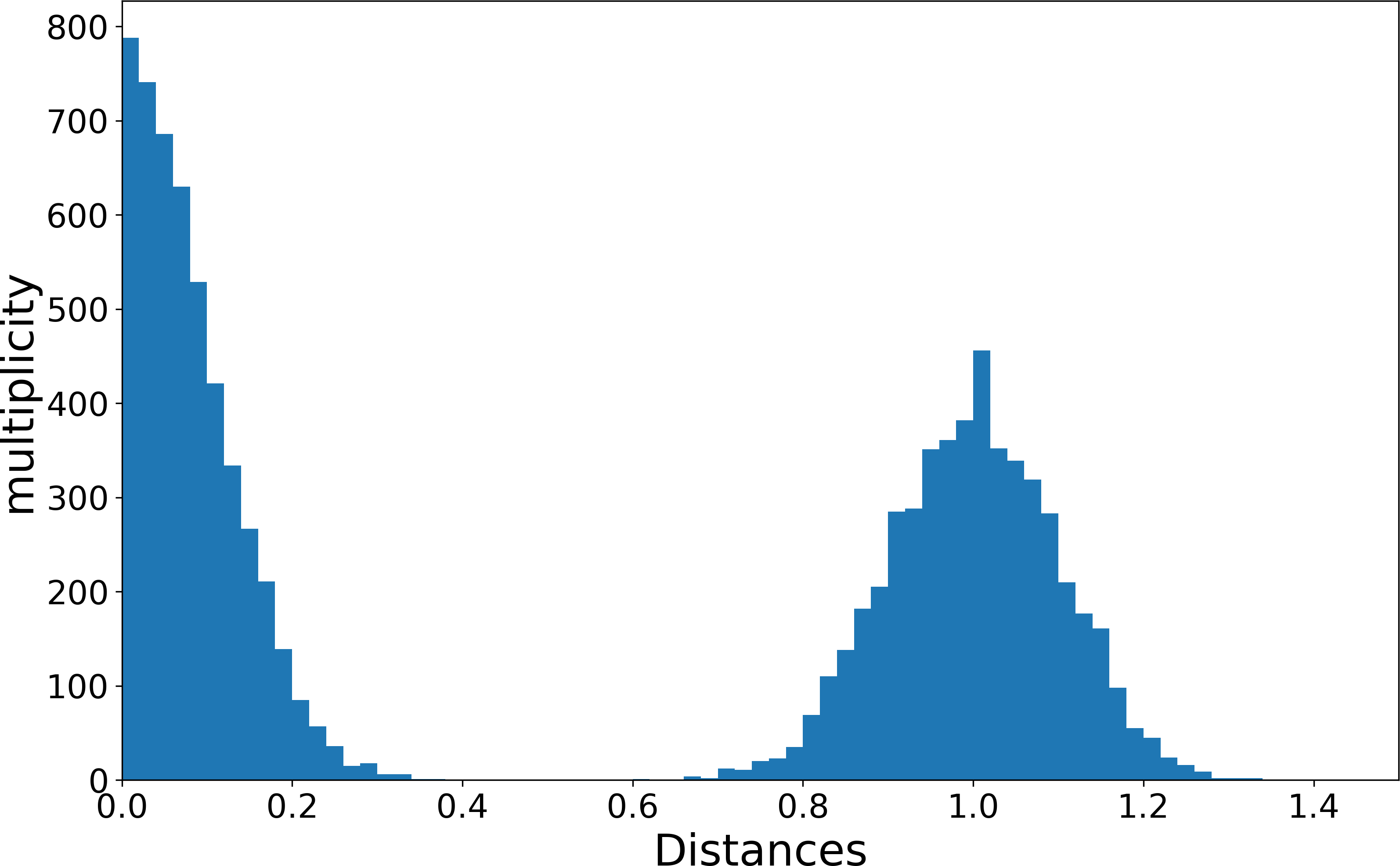
(a) Dimension $p=1$

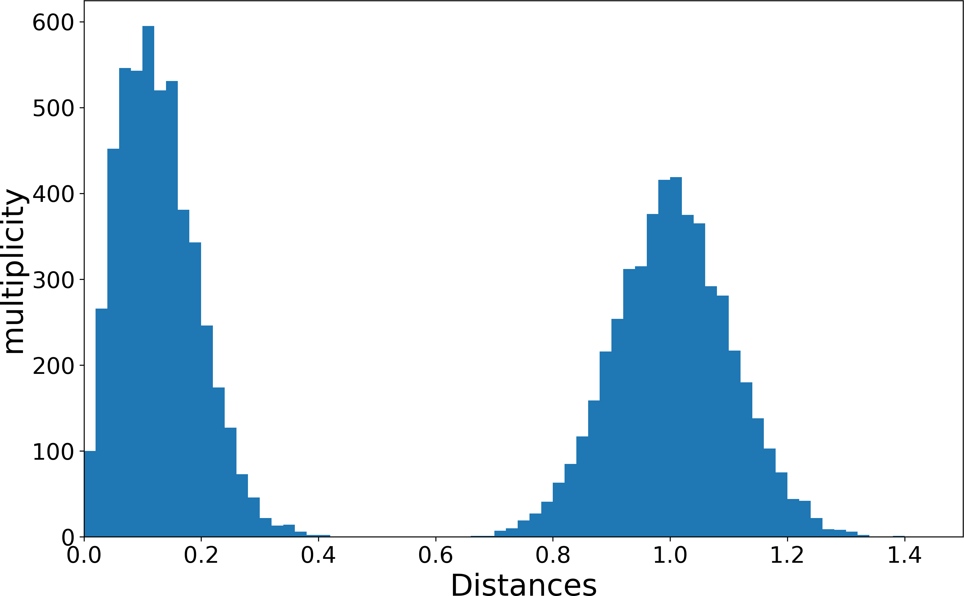
(b) Dimension $p=2$

Figure 1: Typical distributions of $d_{j}$ in case that the population Fréchet function has two minima. In the one-dimensional case, the cluster containing $\widehat{\mu}_{n}$ appears as a falling slope and the second cluster as a full mode. However, in the two-dimensional case, the cluster containing $\widehat{\mu}_{n}$ also appears as a full mode with rising and falling slope due to the volume element. Therefore, it is not sensible to search the first rising slope starting from $0$, but instead we search the next rising slope after the first falling slope.

Now, we have defined all the quantities needed to give a concise definition of the hypothesis tests for non-uniqueness.

Hypothesis Test 4.1.

Null hypothesis and alternative:

• $H_{0}\,:\,|E|\geq 2$, $\quad H_{1}\,:\,|E|=1$.

Test statistics:

• 1) $T_{d}:=\frac{2}{B}|\{d_{j}:d_{j}>d_{+}\}|$.

• 2) $T_{\ell}:=\frac{2}{B}|\{\ell_{j}:\ell_{j}>\ell_{+}\}|$.

Rejection regions and p-values:

• 1) Reject if $T_{d}<\alpha$, p-value $p_{d}=\min\left\{1,T_{d}\right\}$.

• 2) Reject if $T_{\ell}<\alpha$, p-value $p_{\ell}=\min\left\{1,T_{\ell}\right\}$.

From Theorem 3.21 and Remark 3.22 it becomes clear that these test statistics have asymptotically the correct size for $m=2$ and may be conservative otherwise.

4.1 Simulations

In this section we provide numerical results for performance of Hypothesis Tests 4.1 under the null hypothesis for $m=2$ and some alternatives close to the null. The simulations consider Fréchet means on $S^{p}$ with $p\in\{1,2,3,4,5\}$. For the tests in case of the null hypothesis, we use on $S^{1}$ a mixture of two wrapped normal distributions, denoted by $N_{w}$

$$X\sim 0.5N_{w}\left(0,\frac{\pi}{50}\right)+0.5N_{w}\left(\pi,\frac{\pi}{50}\right)$$

which has means $\pm\frac{\pi}{2}$ and for higher dimensions $p>1$ we use, denoting the normal distribution by $N$

$$Y \sim N\left(0,\frac{10^{-6}}{p^{2}}\right) Z \sim U_{S^{p-1}} X \sim\begin{pmatrix}Y\\ \sqrt{1-Y^{2}}Z\end{pmatrix}$$

which has means $(\pm 1,0,\dots,0)^{T}$, i.e. two opposite poles.

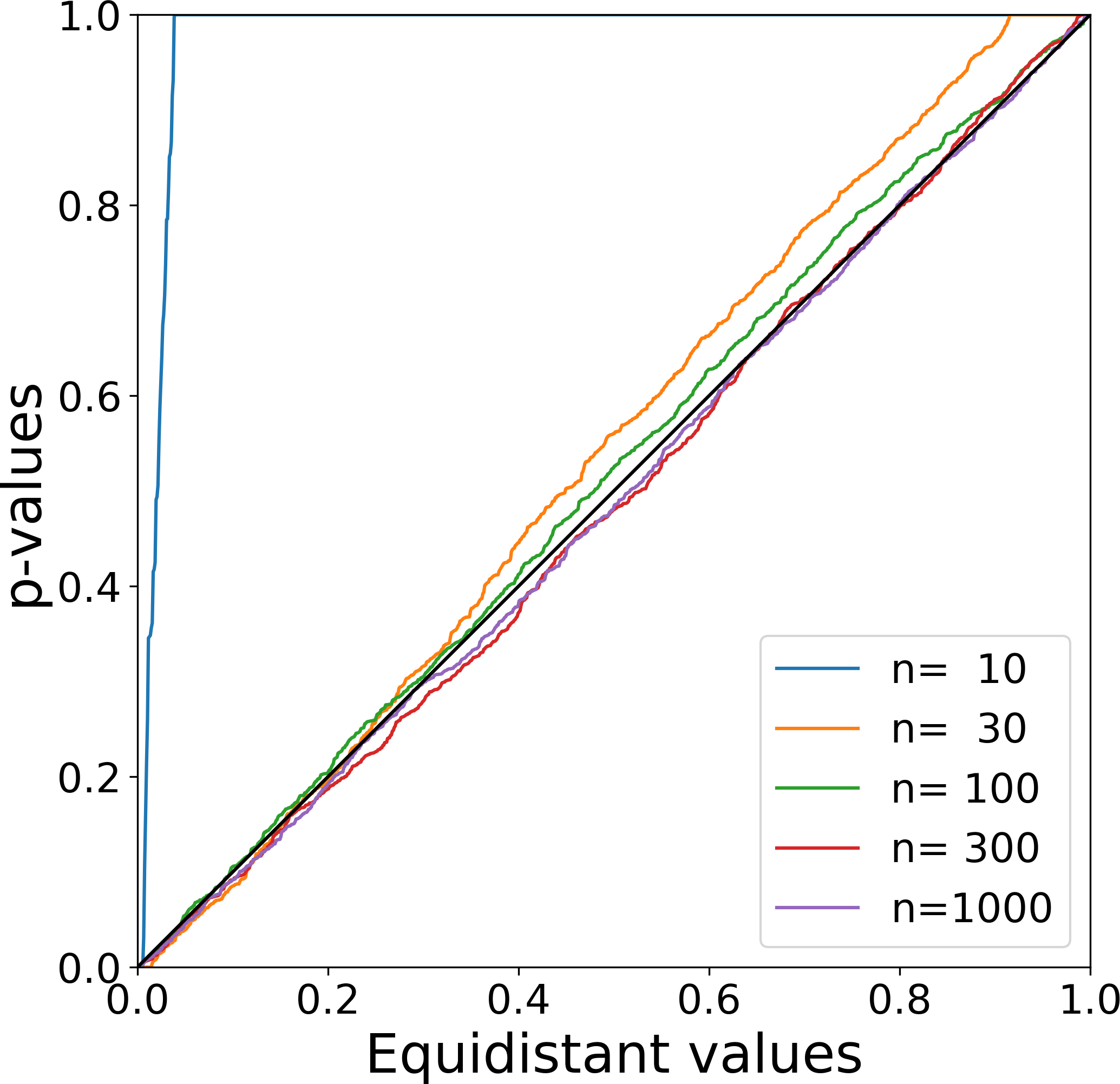
Figure 2: $T=1\,000$ sorted p-values for the null hypothesis in dimension $p=1$ plotted against equidistant values for sample sizes $n=10,30,100,300,1000$. In this case $T_{d}=T_{\ell}$, so no distinction is made. $B=10\,000$ were used for every test. While the test is noticeably conservative for $n=10$ it attains the theoretical size very well for $n\geq 30$.

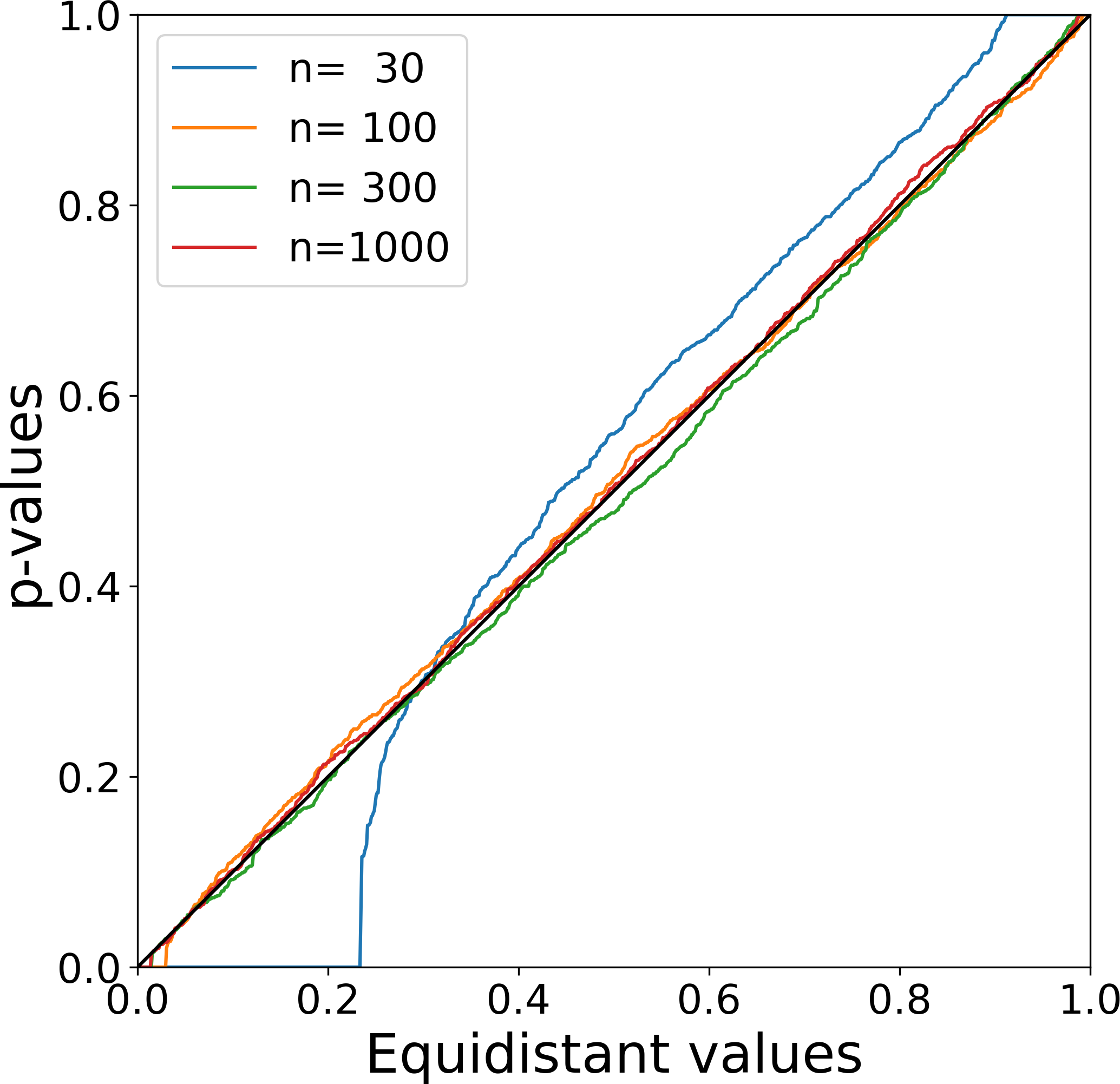
(a) $p_{d}$ for $p=2$

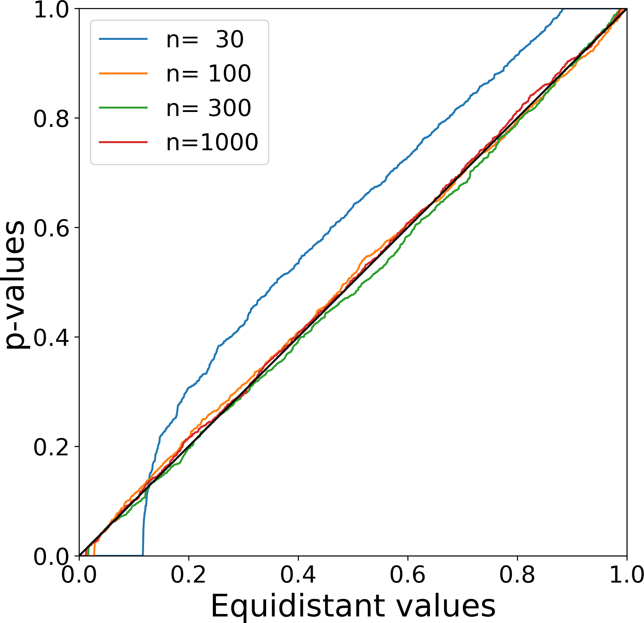
(b) $p_{\ell}$ for $p=2$

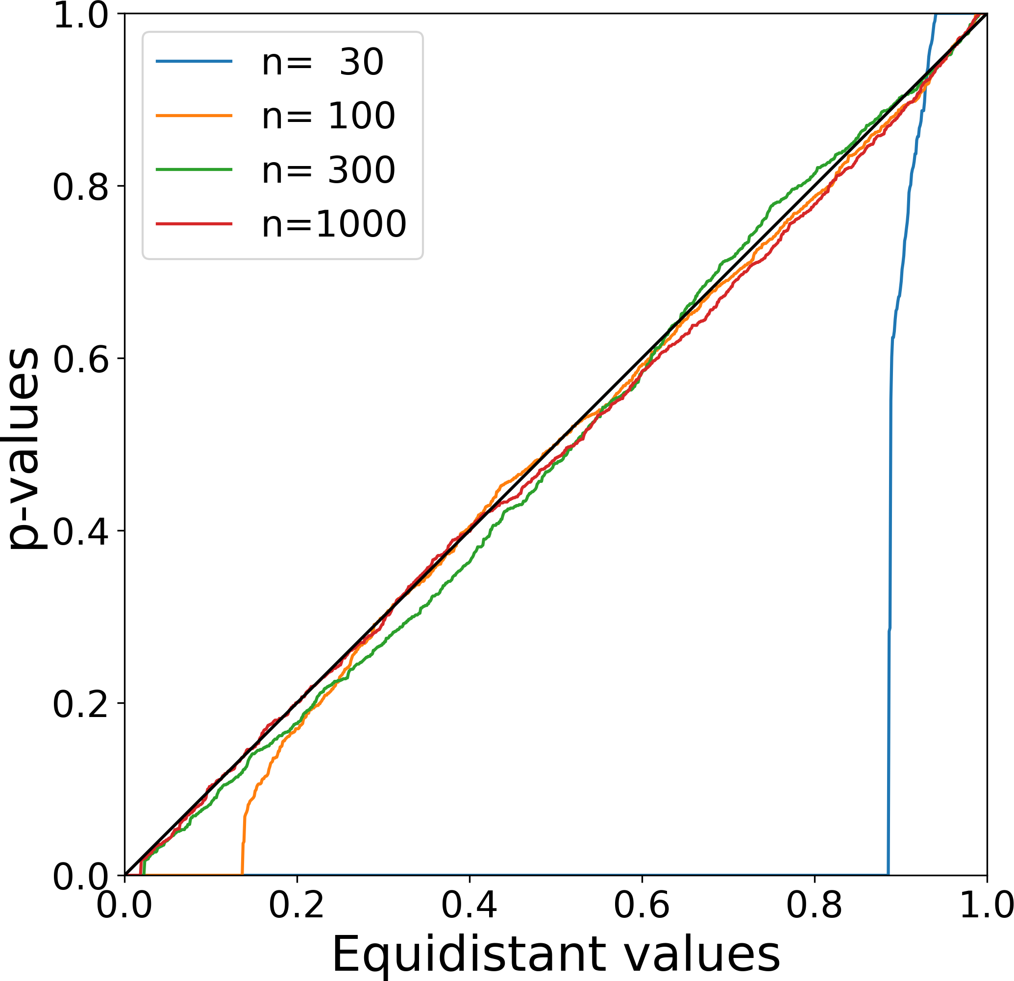
(c) $p_{d}$ for $p=3$

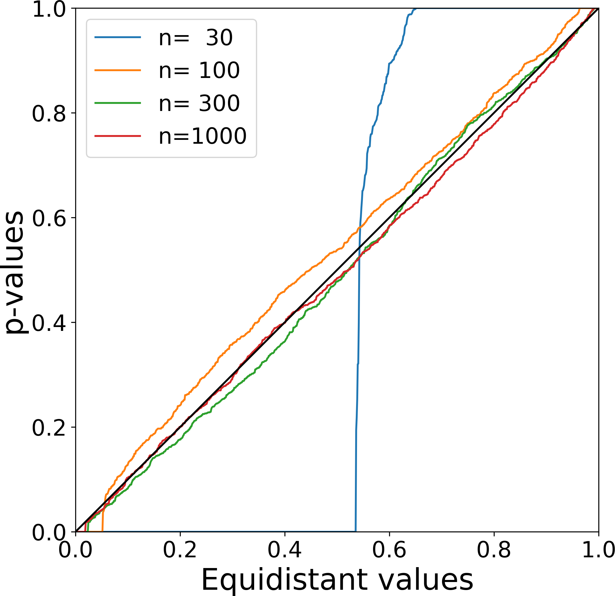
(d) $p_{\ell}$ for $p=3$

Figure 3: $T=1\,000$ sorted p-values for the null hypothesis in dimensions $p=2,3$ plotted against equidistant values for sample sizes $n=30,100,300,1000$. $B=2\,000$ were used for every test. One can see that the test using $T_{\ell}$ performs somewhat better than the test using $T_{d}$. For $p=2$ both tests appear to achieve the correct size for $n\geq 100$, while for $p=3$ it is preferable to have $n\geq 300$.

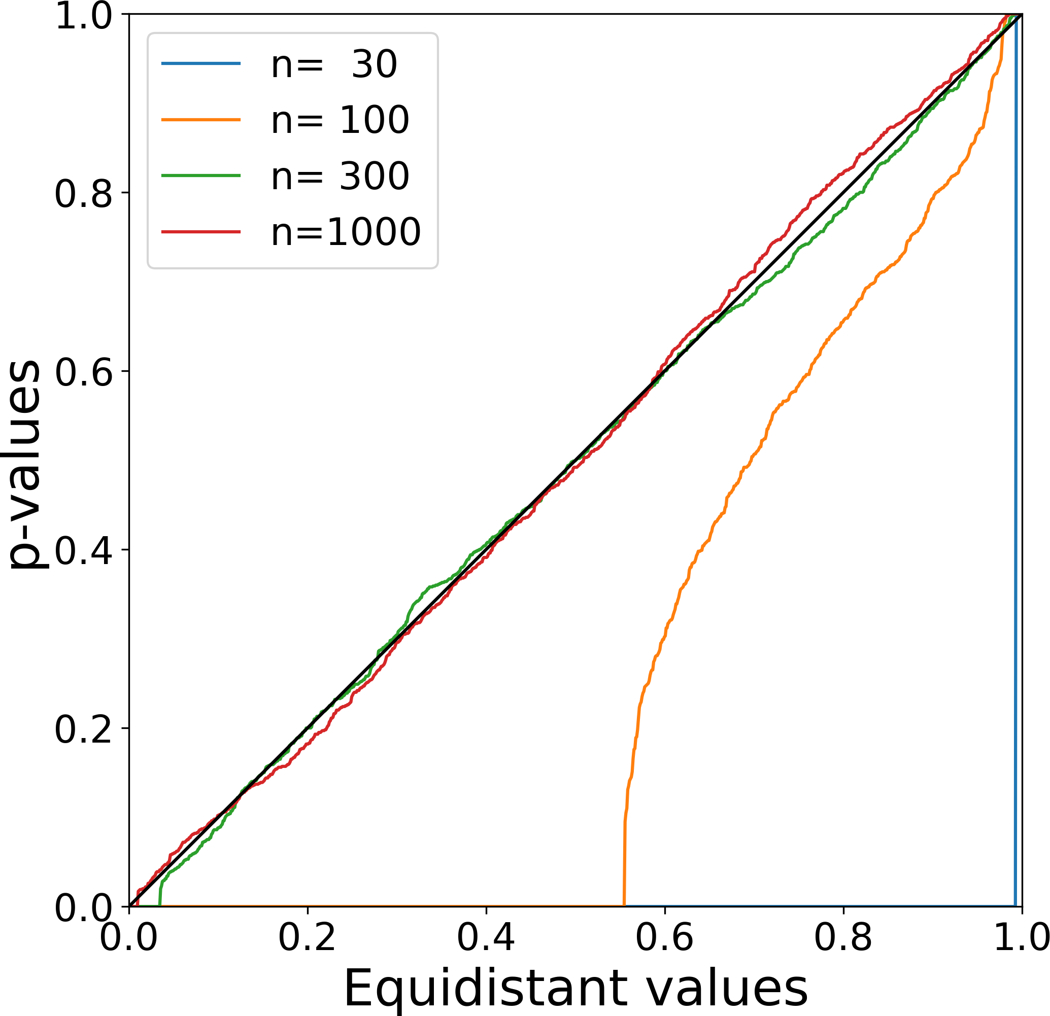
(a) $p_{d}$ for $p=4$

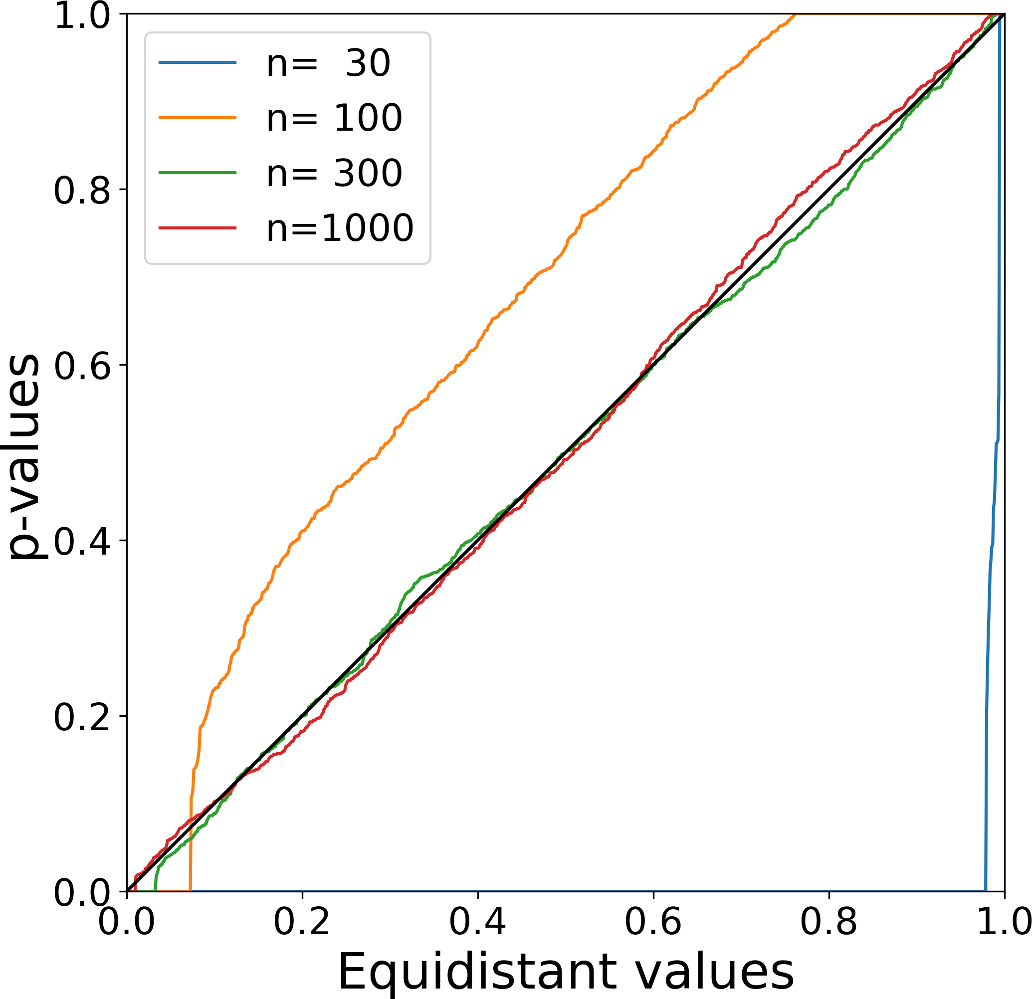
(b) $p_{\ell}$ for $p=4$

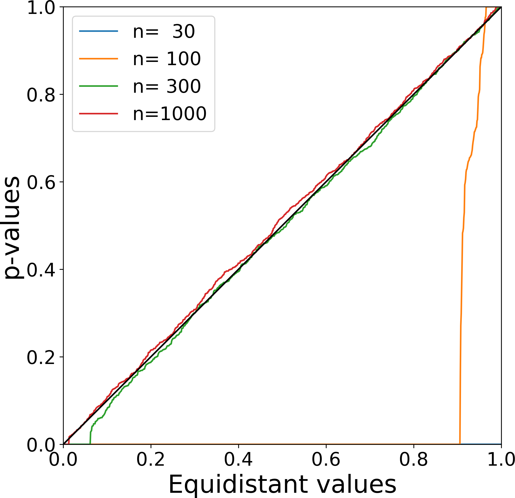
(c) $p_{d}$ for $p=5$

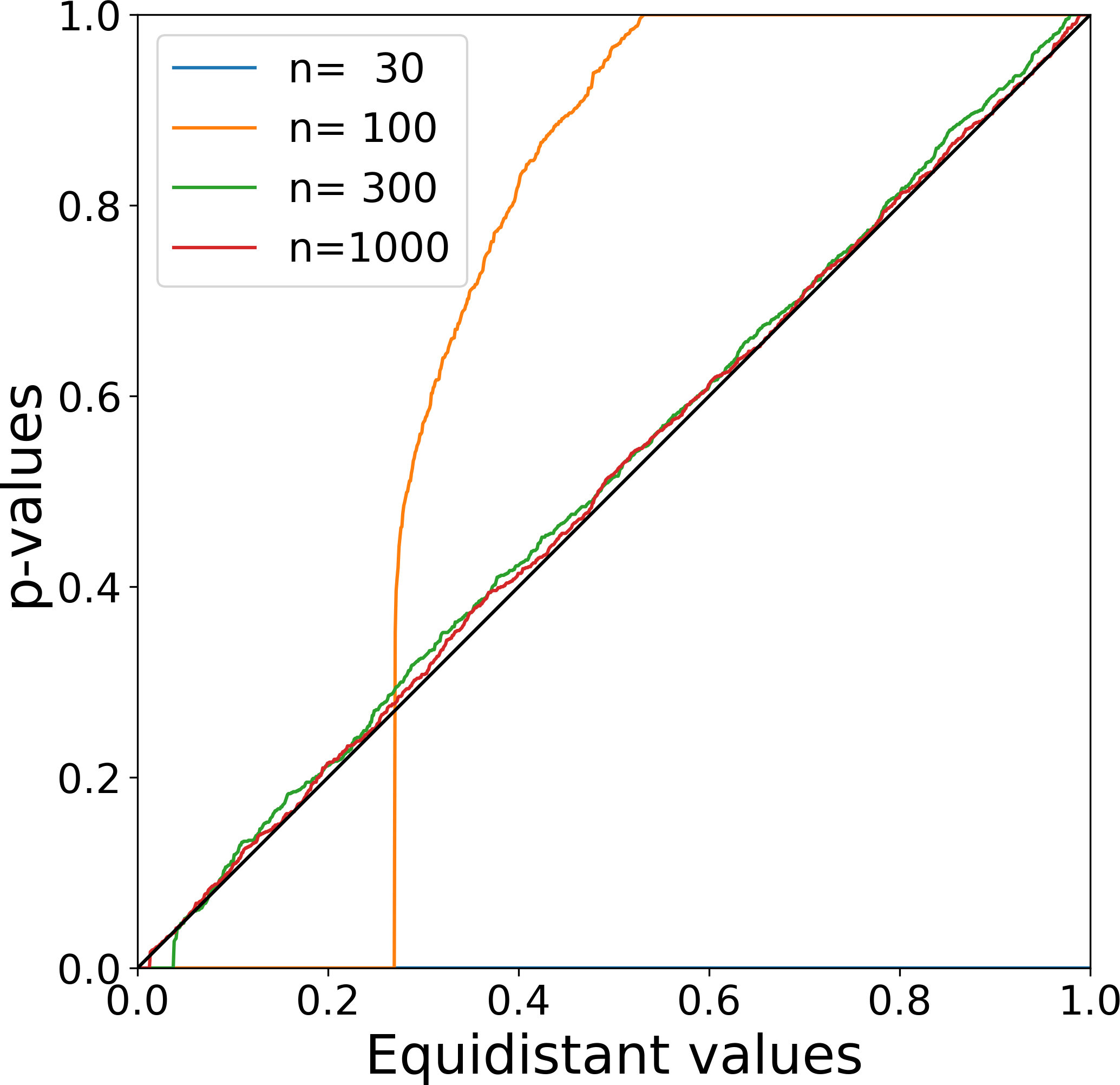
(d) $p_{\ell}$ for $p=5$

Figure 4: $T=1\,000$ sorted p-values for the null hypothesis in dimensions $p=4,5$ plotted against equidistant values for sample sizes $n=30,100,300,1000$. $B=2\,000$ were used for every test. One can see that the test using $T_{\ell}$ performs somewhat better than the test using $T_{d}$. For $p=4$ both tests appear to achieve the correct size for $n\geq 300$, while for $p=5$ it is preferable to have $n\geq 1000$.

For $p=1$ we use $B=10\,000$ and otherwise $B=2\,000$. We then perform tests on $T=1\,000$ samples for each sample size and display the resulting sorted p-valued in a pp-plot in Figures 2, 3 and 4. Generally, we observe that the test statistic $T_{\ell}$ appears to yield somewhat better results than $T_{d}$. Both tests approach the size predicted by the asymptotics for large $n$, and in the one-dimensional situation the test achieves very good performance already for $n=30$.

Since the multiscale test by Dümbgen and Walther (2008) works best if modes consist of $\>\raisebox{1.20007pt}{\vstretch{0.7}{\gtrsim}}\>50$ points, p-values below $0.05$ are often underestimated to be $0$ when $B=1\,000$, therefore it is advisable to use $B=10\,000$ in data applications. Furthermore, we observe that for small sample sizes and $p>1$ many sample means are close to the equator, $e_{1}^{T}\widehat{\mu}_{n}\approx 0$. This effect becomes more pronounced with increasing dimension $p$. Therefore, the tests require increasing sample size with increasing dimension in our setting to avoid being too liberal. In our simulations $n\>\raisebox{1.20007pt}{\vstretch{0.7}{\gtrsim}}\>300$ is sufficient to achieve good performance. In other scenarios dimension dependence can vary but in general greater sample sizes are needed in higher dimension.

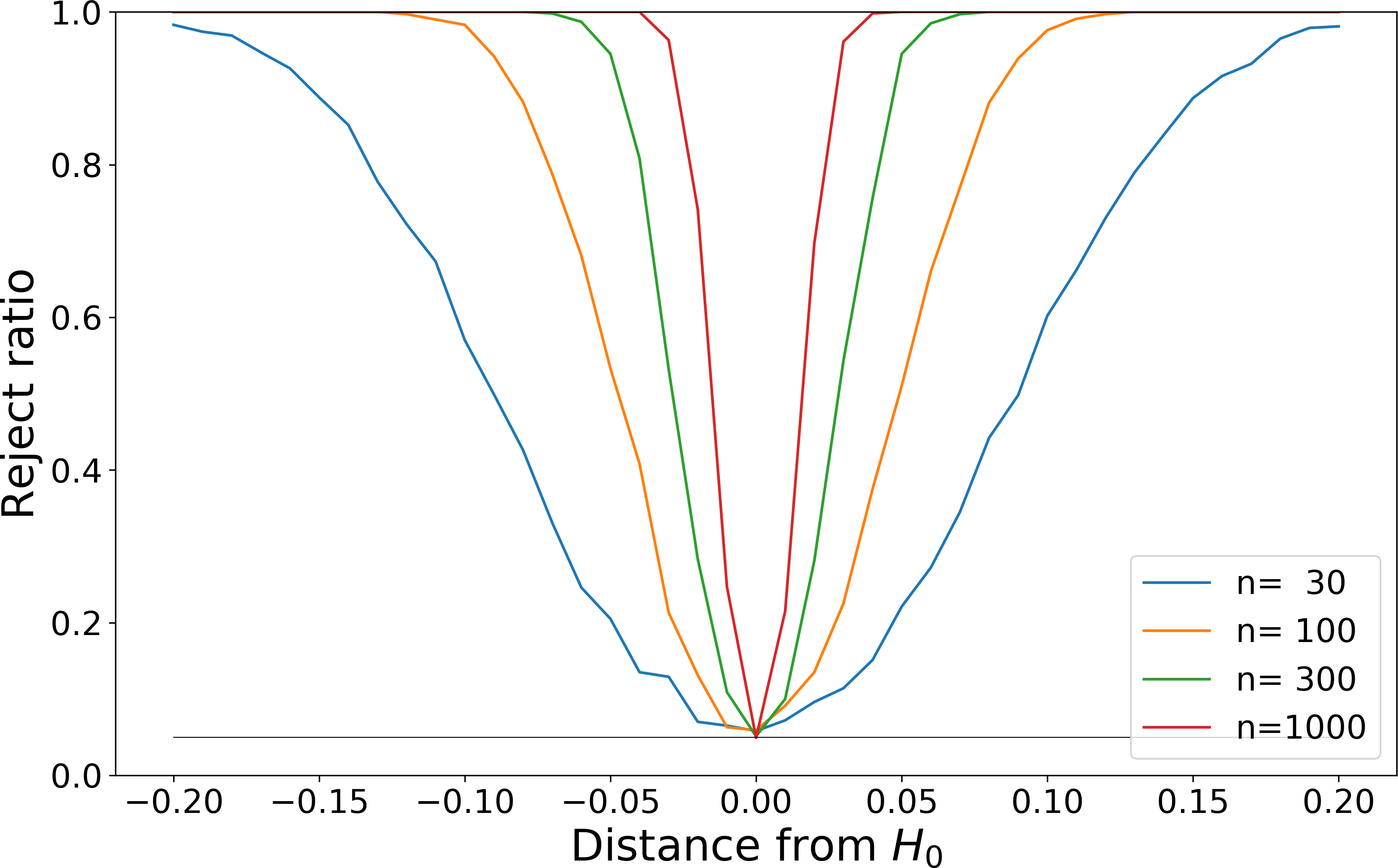
Figure 5: Ratio of rejecting tests for dimension $p=1$ using $T=1\,000$ tests to level $\alpha=0.05$ with $B=2\,000$ bootstrap samples each for distributions close to the null hypothesis as defined in Equation (12). We see that the power increases rapidly with $n$ as expected and the correct size is attained at the null hypothesis for large enough $n$ with good results already for $n=30$.

Next, we investigate the power of the test in dimension $p=1$ for distributions close to the null hypothesis. We use on $S^{1}$ a mixture of two wrapped normal distributions, denoted by $N_{w}$

$$X\sim 0.5N_{w}\left(a,\frac{\pi}{50}\right)+0.5N_{w}\left(\pi-a,\frac{\pi}{50}\right)$$ (12)

where $a\in[-0.1,0.1]$. Note that for $a>0$ the mean is unique $\mu=\pi/2$, for $a<0$ the mean is unique $\mu=-\pi/2$ and for $a=0$ the mean is non-unique $\mu=\pm\pi/2$,.

The numerical results for the power of the test are displayed in Figure 5. The test can clearly discern the tested alternative from the null in the tested family of distributions. The power of the test increases appreciably with $n$, as one would expect. These numerical results illustrate that test is suited for its purpose and is for low dimensions already reliably applicable for fairly low $n$.

4.2 Application to Data

In this Section, we apply Hypothesis Test 4.1 to various data examples to illustrate its range of applicability. The examples comprise the Fréchet mean on manifolds, non-linear regression and clustering. The interpretation of test results varies according to the data application and is highlighted in each example for clarity.

4.2.1 Nesting Sea Turtles

First we will look at the classic example of the mean on the circle. We consider the classic “turtles” data set from Mardia and Jupp (2000, p. 9), which gives the compass directions under which $n=76$ female turtles leave their nests after egg laying.

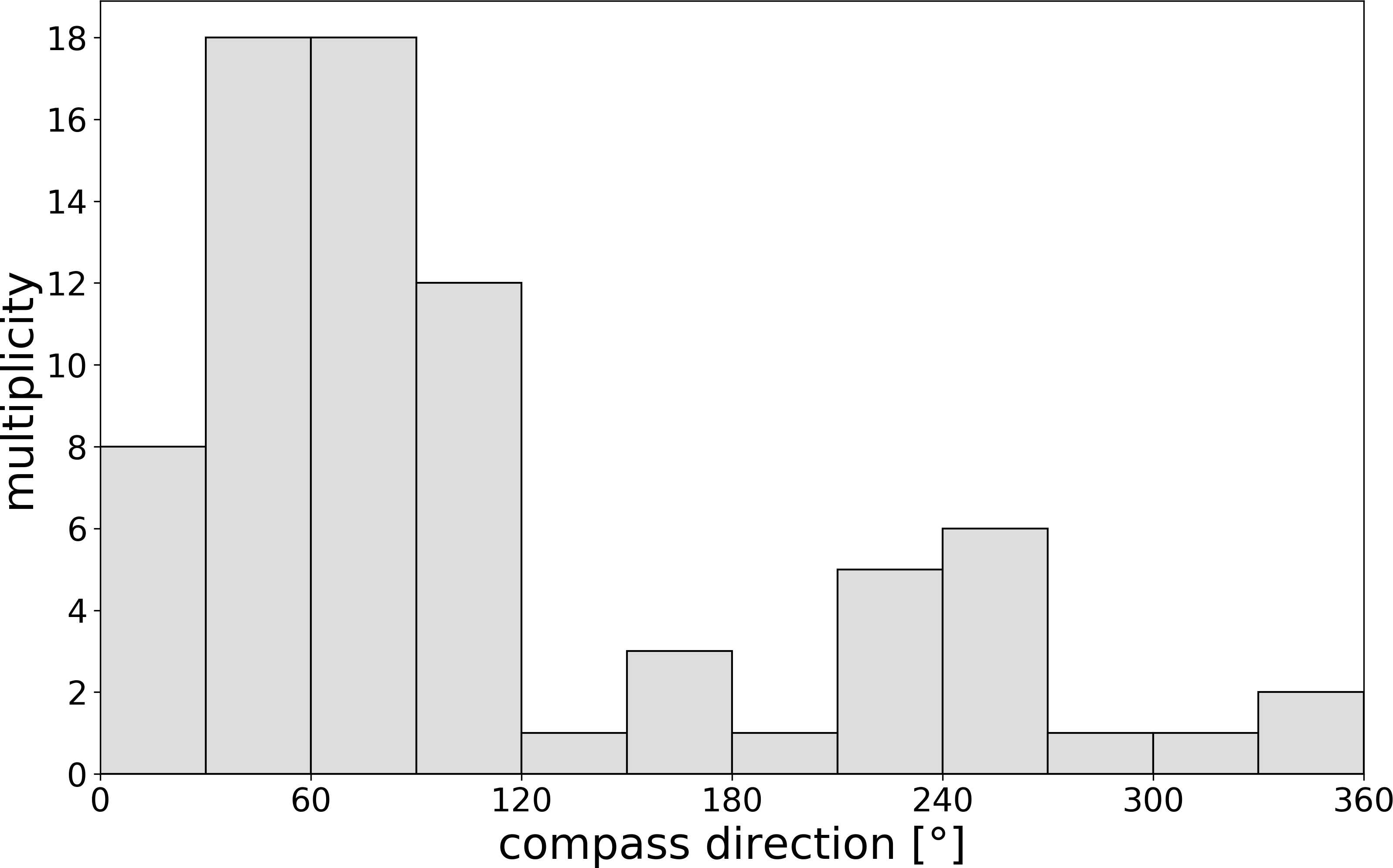
(a) histogram of turtle directions

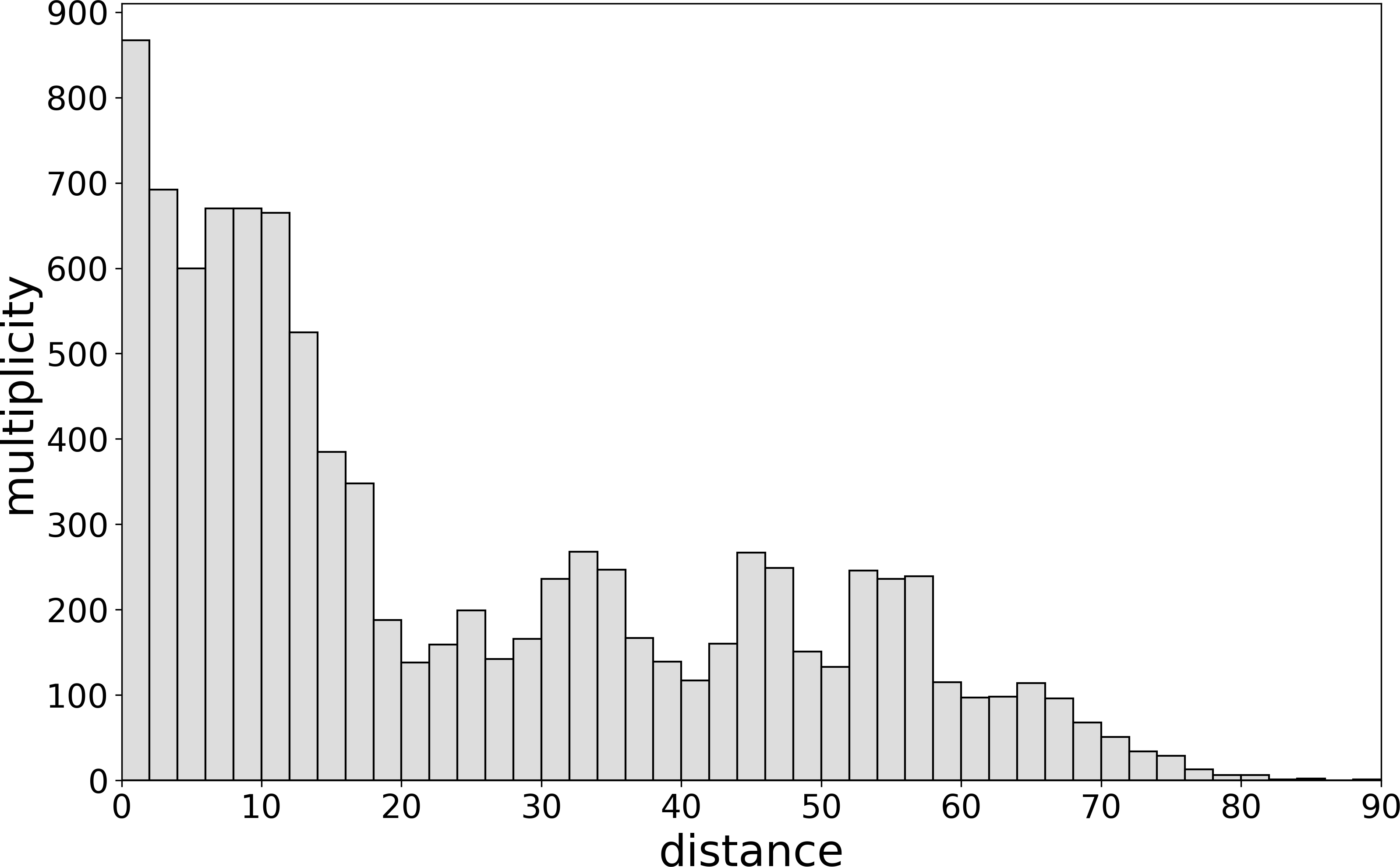
(b) histogram of bootstrap mean distances $d_{j}$

Figure 6: Illustration of the turtle data and the results of the bootstrap with $B=10\,000$. Panel (a) shows a pronounced bimodal structure of the data and panel (b) shows that this leads to several secondary modes in the distribution of bootstrap means. This already indicates that the test will likely not reject the null hypothesis for this data set. Due to the small $n$, the number of minima $m$ of the underlying population cannot be easily determined in this case.

The data and the bootstrap histogram used for the hypothesis test are illustrated in Figure 6. Indeed the hypothesis test with $B=10\,000$ yields a p-value of $0.7868$, which means that the hypothesis that the mean is not unique cannot be rejected.

Interpretation 4.2.

The data set was previously investigated for finite sample smeariness, as defined by Hundrieser et al. (2020), in Eltzner and Huckemann (2019) where it was shown to exhibit very pronounced finite sample smeariness. Indeed, due to the fact that the limiting distribution of the mean in case of smeariness is not unimodal, the test for non-uniqueness of the mean can be expected not to reject in case of finite sample smeariness. This is desirable, since smeariness occurs generically as a boundary case between distributions with a unique mean and distributions with non-unique mean. The data set is therefore compatible with a smeary mean of the population as well as with non-unique mean.

4.2.2 Platelets Spreading on a Substrate

The second data set we are considering was first presented in Paknikar et al. (2019). The data describe the total length $\ell$ of actin stress-fiber-like structures in blood platelets over time $t$ during spreading on a substrate. The expected behavior is an initial growth of fiber structures which is completed after a certain growth time. This leads to a regression problem with a more involved m-estimator. Consider two-dimensional data $x:=(t,\ell)$, four parameters $\theta:=(\theta_{1},\theta_{2},\theta_{3},\theta_{4})\in\mathbb{R}\times\mathbb{R}^{+}\times\mathbb{R}\times\mathbb{R}$ and the loss function

$$f(t,\theta):= \max\left\{0,(\theta_{3}+\theta_{4}t)\cdot\left(1-\exp\left(\theta_{1}-\frac{t}{\theta_{2}}\right)\right)\right\}$$

$$\rho(x,\theta):= \left(\ell-f(t,\theta)\right)^{2}$$

which amounts to a standard quadratic loss regression model with a somewhat unusual four-parametric regression function $f$. However, since this loss function is treated in an m-estimator setting, the theory and test laid out in this paper can be applied in this setting. The parameter $\theta_{2}$ describes the time scale of fiber growth and is therefore the parameter of greatest interest.

Since imaging on such small scales and such high time resolution is very challenging, images frequently feature low brightness and some blurring, which in turn poses a challenge for image analysis. The semi-automated line detection using the Filament Sensor Eltzner et al. (2015) comes with some amount of artifacts which lead to a high variance of $\ell$. As a results, for some of the platelets several local minima of the sample loss exist and our test with $B=10\,000$ shows that these can sometimes not be rejected as valid minima of population loss.

The distance between two sets of parameters is defined via $L^{2}$ distance of the curves within the experimental time $[0,T]$, where we use a simple sum approximation to reduce calculation time.

$$d(\theta,\widetilde{\theta}):=T^{2}\int_{0}^{T}\limits|f(t,\theta)-f(t,\widetilde{\theta})|^{2}dt\approx\sum_{i=1}^{n}|f(t_{i},\theta)-f(t_{i},\widetilde{\theta})|^{2}$$

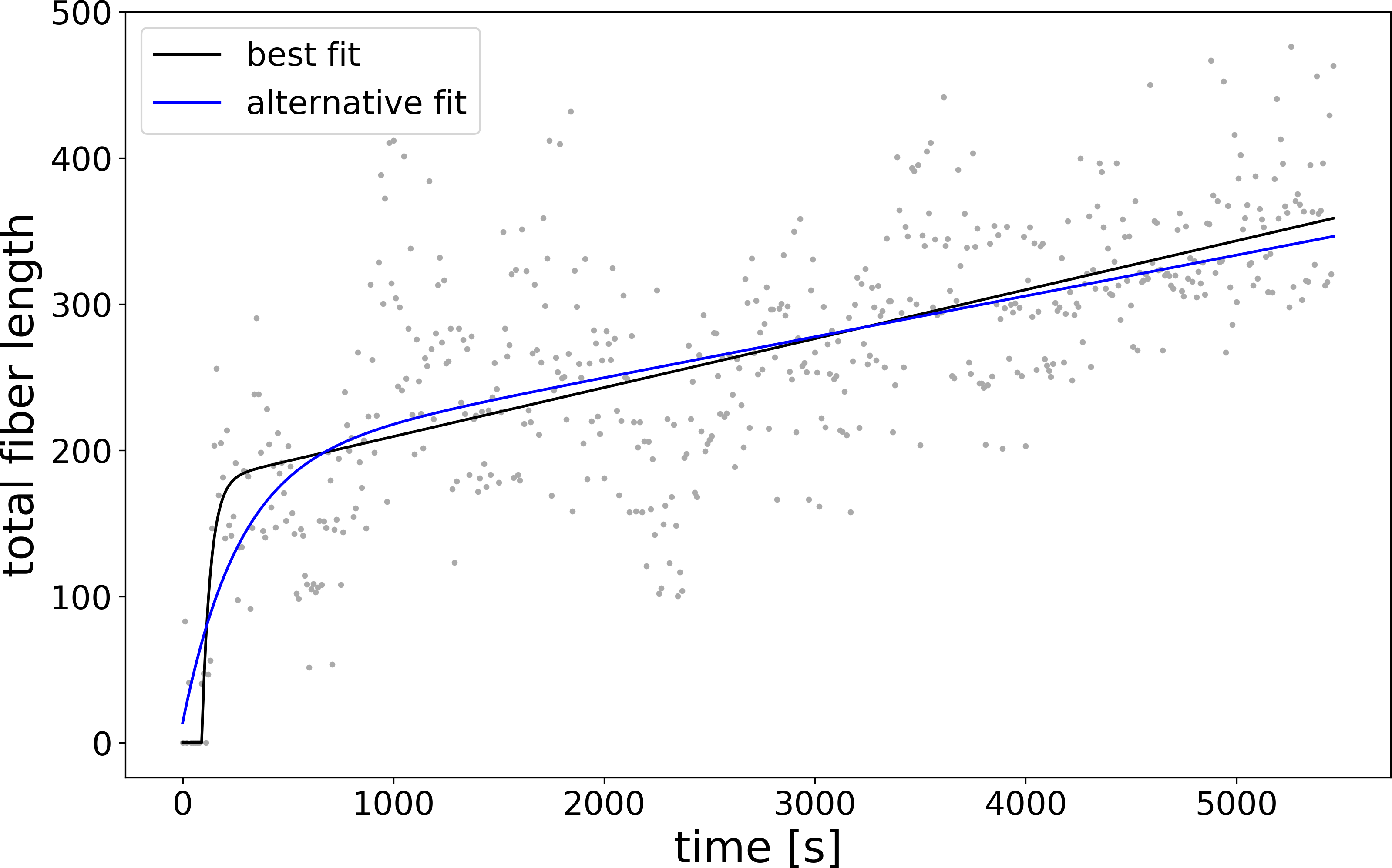
(a) Test rejects with $p_{d}=0.2270$

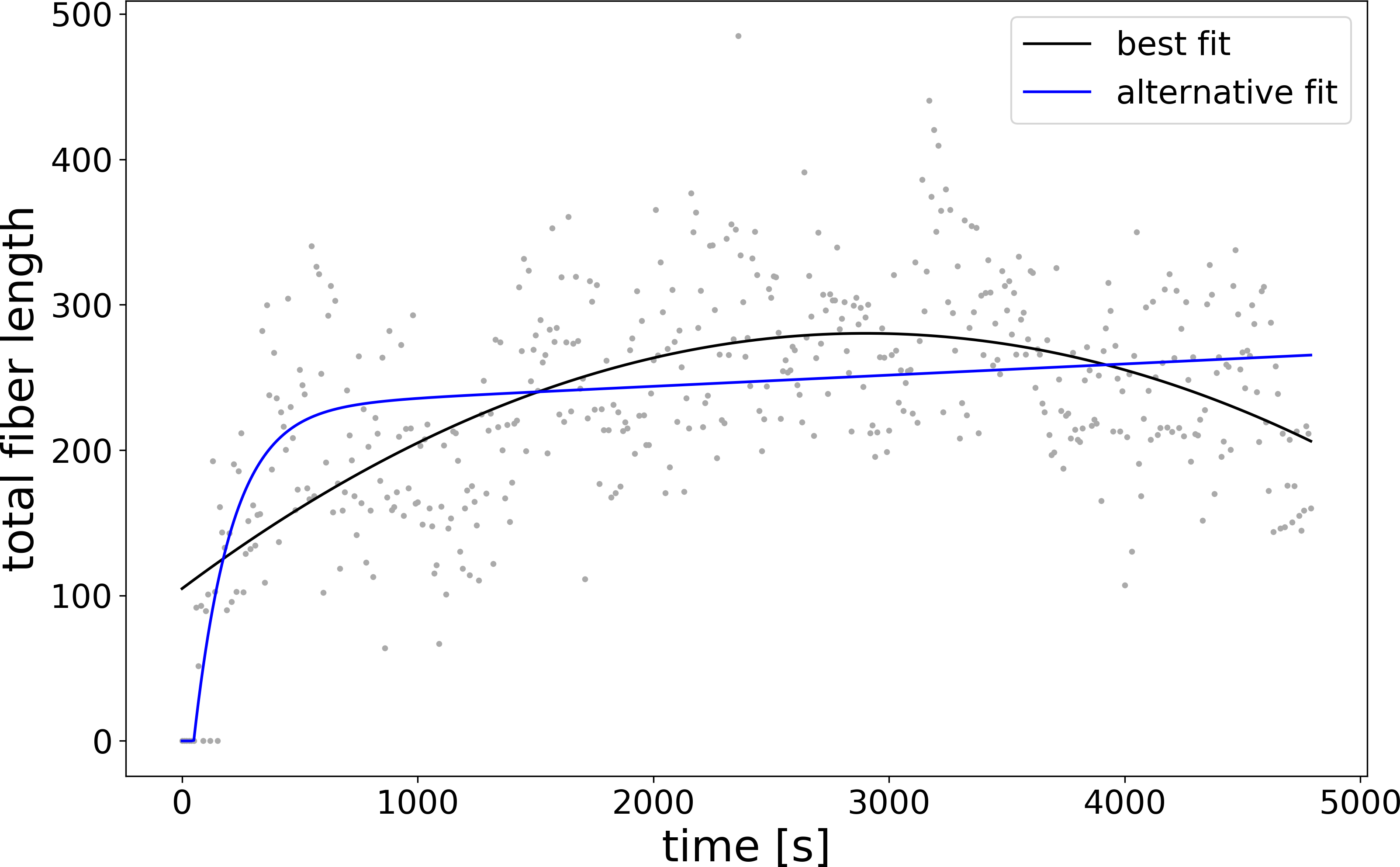
(b) Test does not reject with $p_{d}=0.0438$

Figure 7: Plots for two of the time series. Panel (a) displays a typical example, where the test does not reject the possibility for a second valid optimal fit. The fits are very similar for long times but differ more strongly at short times. Panel (b) displays an extreme case, in which the best fit leads to extreme parameter values and an unusual curve shape. The test does not reject in this case because the secondary cluster is small, however the alternative fit looks much closer to an expected result. In this case, it can be beneficial to restrict the parameter space. In Paknikar et al. (2019) the restriction $\theta_{1}\theta_{2}\geq-30$ was used, since the begin of spreading, marked by the initial departure of the curve from $0$, must be within the movie or very briefly before due to the experimental setup.

In Figure 7 we show two examples. Panel (a) displays a typical example where the fact that the test does not reject indicates a non-unique optimum.

Interpretation 4.3.

In the example in panel (b) the best fit violates assumptions of the experiment, namely the fact that the movies are started once the platelet begins spreading on the substrate and this the begin of spreading can at most lie a few seconds before the start of the time series. Therefore, this fit suggests that restricting parameter space to $\theta_{1}\theta 2\geq-30$ as done by Paknikar et al. (2019) is necessary here.

The results of Paknikar et al. (2019) concerning the time scale of actin fiber formation remains mostly unaffected by the result presented here, since only five platelet in the full data set exhibit non-uniqueness in their fits and only for two this remains true if the parameter space is restricted to $\theta_{1}\theta 2\geq-30$. In these two cases, the two candidates for the optimum have very similar time constants $\theta_{2}$.

4.2.3 Gaussian Mixture Clustering

For a third example, we consider centroid based clustering of data on $\mathbb{R}^{2}$. In the examples presented here, we use a Gaussian mixture model and apply an EM algorithm for the optimization. We use two classic data sets which are provided by the GNU R datasets package.

The faithful data set contains eruption duration and preceding inactivity of $n=272$ eruptions of the Old Faithful geyser in Yellowstone national park. The data set is famously bimodal and the fit of a two-cluster mixture model clearly rejects the hypothesis of non-uniqueness with a p-value of $0$ according to both test statistics with $B=10\,000$. However, when fitting a three-cluster mixture model, which can be considered overfitting, both tests no longer reject, with p-values $p_{d}=0.6804$ and $p_{\ell}=0.655$. This reinforces the notion that three clusters cannot be uniquely fit to the data in a meaningful way.

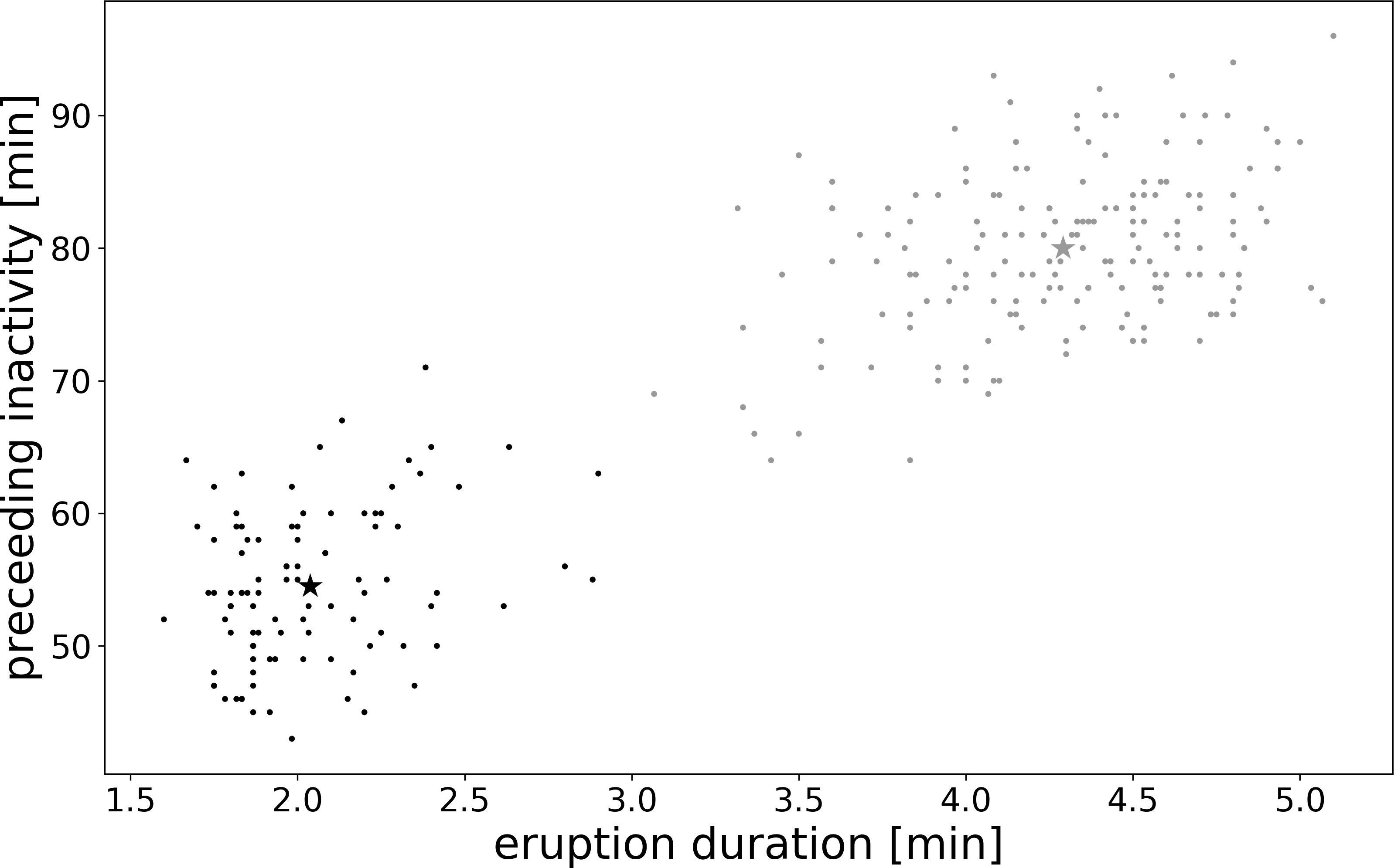
Figure 8: Scatter plot of old faithful eruption data with colors indicating the two-cluster segmentation and the stars indicating cluster centers.

The iris data set is a widely used benchmark and illustration data set for classification methods. It contains measurements of $4$ features of $50$ iris blossoms fore each of three different species, leading to an overall sample size of $n=150$ of data in $\mathbb{R}^{4}$. One of the three species forms a clearly distinct cluster, which can be easily identified. However, the clusters of the two other species have some overlap and it is not immediately clear from the data, whether three clusters should be fit to the data. A two-cluster model fits the data very well and our tests reject with p-values of $0$ with $B=10\,000$. However, when fitting three clusters we find p-values $p_{d}=p_{\ell}=1$, so the tests do not reject the possibility of multiple minima. This indicates that the three-cluster Gaussian mixture segmentation of the data set is unreliable and more data are needed for a unique result.

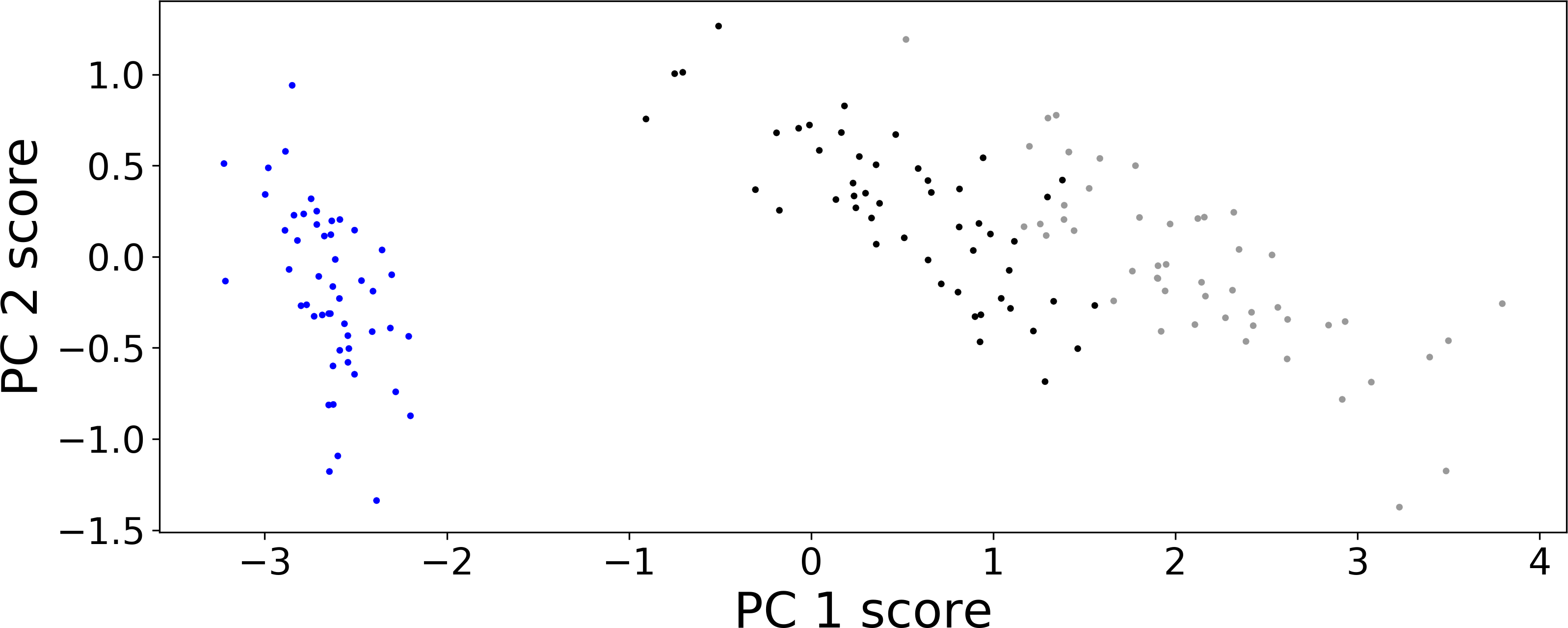
(a) species labels

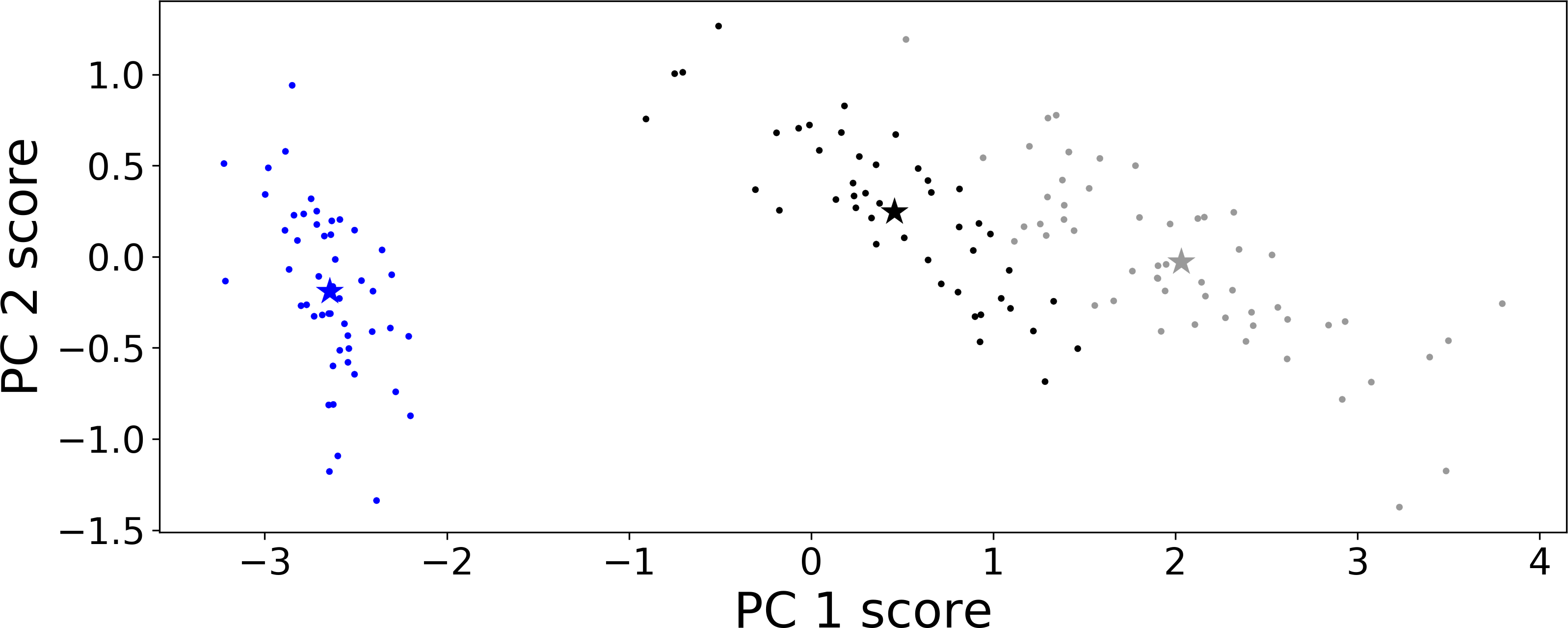
(b) Gaussian mixture clusters

Figure 9: Scatter plots of the first two principal components of the iris blossom data. The colors in panel (a) highlight the three species, while the colors in panel (b) show the three clusters and their centers in the three-cluster segmentation. The clustering results are in very good agreement with the true labels. However, the fact that our hypothesis test does not reject the hypothesis that another clustering result may be equally valid calls the significance of this result into question.

Interpretation 4.4.

For the simple Gaussian mixture clustering, which can be interpreted as an unsupervised classification algorithm, we find that the result assuming two components yields a unique result for both data sets. Since the faithful data set consists of two modes, the results that the fit with three components is ambiguous is expected. The iris data set, however, consists of three subsets and a clustering assuming three components reflects the true labels surprisingly well. However, the test for non-uniqueness leads one to question the reliability of the result, since the existence of an alternate “best fit” for the population is not ruled out. This is an example for how the test for non-uniqueness of descriptors can be used to indirectly determine the optimal number of clusters.

Appendix A Test Size for Fréchet Function with $m$ Minima

Consider a random vector $X\sim N(0,\Sigma)$ and for any $i,j\in\{1,2,\dots,m\}$ with $i\neq j$ let $e_{ij}:=(e_{i}-e_{j})$. Define the following sets

$$A^{\alpha}_{ij} =\left\{x\in\mathbb{R}^{m}:e_{ij}^{T}x\leq\left(e_{ij}^{T}\Sigma e_{ij}\right)^{1/2}q\left(\frac{\alpha}{2}\right)\right\} A^{\alpha}_{i}:= \bigcap_{\begin{subarray}{c}j=1\\ j\neq i\end{subarray}}^{m}\limits A^{\alpha}_{ij}\,.$$

Theorem A.1.

Let $X\sim N(0,\Sigma)$ be a multivariate normal random vector in $\mathbb{R}^{m}$ for $m\in\{2,3\}$. Then for all $\alpha\in[0,1]$

$$\sum_{i=1}^{m}\limits\mathbb{P}\left(A^{\alpha}_{i}\right)\leq\alpha$$

Proof.

For $m=2$ we get $\sum_{i=1}^{2}\limits\mathbb{P}\left(A^{\alpha}_{i}\right)=\mathbb{P}\left(A^{\alpha}_{12}\right)+\mathbb{P}\left(A^{\alpha}_{21}\right)=\alpha$.

For $m=3$ we get

$$\sum_{i=1}^{3}\limits\mathbb{P}\left(A^{\alpha}_{i}\right)= \mathbb{P}\left(A^{\alpha}_{12}\cap A^{\alpha}_{13}\right)+\mathbb{P}\left(A^{\alpha}_{21}\cap A^{\alpha}_{23}\right)+\mathbb{P}\left(A^{\alpha}_{13}\cap A^{\alpha}_{23}\right)$$

$$= \mathbb{P}\left(A^{\alpha}_{12}\cap A^{\alpha}_{13}\right)+\mathbb{P}\left(A^{\alpha}_{21}\cap A^{\alpha}_{13}\cap A^{\alpha}_{23}\right)+\mathbb{P}\left((A^{\alpha}_{21}\cup A^{\alpha}_{13})\cap A^{\alpha}_{23}\right)$$

$$= \mathbb{P}\left((A^{\alpha}_{12}\cup(A^{\alpha}_{21}\cap A^{\alpha}_{23}))\cap A^{\alpha}_{13}\right)+\mathbb{P}\left((A^{\alpha}_{21}\cup A^{\alpha}_{13})\cap A^{\alpha}_{23}\right)$$

$$\leq \mathbb{P}\left(A^{\alpha}_{13}\right)+\mathbb{P}\left(A^{\alpha}_{23}\right)=\alpha\,.$$

∎

Theorem A.2.

Let $X\sim N(0,\Sigma)$ be a multivariate normal random vector in $\mathbb{R}^{m}$ for $m\geq 4$. Then for sufficiently small $\alpha\geq 0$

$$\sum_{i=1}^{m}\limits\mathbb{P}\left(A^{\alpha}_{i}\right)\leq\alpha\,,$$

Proof.

Define the functions

$$f_{i}:\alpha\mapsto\frac{1}{(2\pi)^{\frac{m}{2}}(\det\Sigma)^{1/2}}\int_{A^{\alpha}_{i}}\limits\exp\left(-\frac{1}{2}x^{T}\Sigma^{-1}x\right)\,dx\,.$$

The claim follows, if $f_{i}^{\prime}(0)=0$ for all $i$, therefore we will show this. In order to simplify calculations, we make a basis transform to “homoscedastic coordinates”. Let $\widetilde{v}_{ij}:=\Sigma^{1/2}e_{ij}$, $v_{ij}:=\frac{\widetilde{v}_{ij}}{|\widetilde{v}_{ij}|}$ and $\widetilde{y}:=\Sigma^{-1/2}x$. Let $e_{0}:=\frac{1}{\sqrt{m}}\sum_{i=1}^{m}\limits e_{i}$ and define

$$H_{i}:= \begin{pmatrix}\Sigma^{1/2}e_{0}&v_{i1}&\dots&v_{i(i-1)}&v_{i(i+1)}&\dots&v_{im}\end{pmatrix}^{T} w_{i}:= H_{i}^{-1}\begin{pmatrix}0&1&\dots&1\end{pmatrix}^{T}\,.$$

This allows us to define $y:=\widetilde{y}-w_{i}q\left(\frac{\alpha}{2}\right)$. Then, the following sets are equivalent to the $A^{\alpha}_{ij}$ defined above

$$B^{\alpha}_{ij}:= \left\{\widetilde{y}\in\mathbb{R}^{m}:v_{ij}^{T}\widetilde{y}\leq q\left(\frac{\alpha}{2}\right)\right\} B^{\alpha}_{i}:= \bigcap_{\begin{subarray}{c}j=1\\ j\neq i\end{subarray}}^{m}\limits B^{\alpha}_{ij}\,.$$

We note that $\widetilde{y}\in B^{\alpha}_{i}\,\Leftrightarrow\,y\in B^{1}_{i}$. We can now introduce shorthand notation and express the above defined functions $f_{i}$ as

$$\exp_{i}(y,\alpha):= \exp\left(-\frac{1}{2}\left|y+w_{i}q\left(\frac{\alpha}{2}\right)\right|^{2}\right) f_{i}(\alpha)= \frac{1}{(2\pi)^{\frac{m}{2}}}\int_{B^{1}_{i}}\limits\exp_{i}(y,\alpha)\,dy\,.$$

In the following we suppress the arguments of $q$ and $\exp_{i}$ to calculate the derivative with respect to $\alpha$

$$f_{i}^{\prime}(\alpha) =-\frac{q^{\prime}}{2(2\pi)^{\frac{m}{2}}}\int_{B^{1}_{i}}\limits w_{i}^{T}\left(y+w_{i}q\right)\exp_{i}\,dz$$

To simplify this expression we define the boundary of $B^{1}_{i}$ as

$$\partial B^{1}_{ij}:= \big{\{}y\in B^{1}_{i}:v_{ij}^{T}y=0\big{\}}\,, \partial B^{1}_{i}:= \bigcup_{\begin{subarray}{c}j=1\\ j\neq i\end{subarray}}^{m}\partial B^{1}_{ij}\,,$$

and we use the fact that for every $j\neq i$ we have $w_{i}^{T}v_{ij}=1$. Then, we get by applying Gauss’ integral theorem, substituting $y=-qz$ (note that $q<0$ for $\alpha<1$) and using $q^{\prime}=(2\pi)^{1/2}\exp\left(\frac{1}{2}q^{2}\right)$ we get

$$f_{i}^{\prime}(\alpha) =\frac{q^{\prime}}{2(2\pi)^{\frac{m}{2}}}\int_{B^{1}_{i}}\limits\textnormal{div}_{y}\big{(}w_{i}\exp_{i}\big{)}\,dy=\frac{q^{\prime}}{2(2\pi)^{\frac{m}{2}}}\int_{\partial B^{1}_{i}}\limits\exp_{i}\,dy$$

$$=\frac{(-q)^{m-1}}{2(2\pi)^{\frac{m-1}{2}}}\int_{\partial B^{1}_{i}}\limits\exp\left(-\frac{1}{2}\left((z-w_{i})^{2}-1\right)q^{2}\right)dz\,.$$

Let $p_{i}:=\operatorname{\mbox{\rm argmin}}_{p\in B_{i}^{1}}\limits|p-w_{i}|$ and note that we have $|p_{i}-w_{i}|^{2}=:1+\delta_{i}>1$. Furthermore, let

$$C_{i}:= \left\{z\in\mathbb{R}^{m}:(w_{i}-p_{i})^{T}z\leq 0\right\} \partial C_{i}:= \left\{z\in\mathbb{R}^{m}:(w_{i}-p_{i})^{T}z=0\right\}$$

where, according to Lemma A.3, $B_{i}\subset C_{i}$ and $p_{i}\in\partial C_{i}$ and for $z\in\partial C_{i}$, one has $(z-w_{i})^{2}=(z-p_{i})^{2}+(p_{i}-w_{i})^{2}$. Then we calculate,

$$f_{i}^{\prime}(\alpha)\leq \frac{(-q)^{m-1}}{2(2\pi)^{\frac{m-1}{2}}}\int_{\partial C^{1}_{i}}\limits\exp\left(-\frac{1}{2}\left((z-w_{i})^{2}-1\right)q^{2}\right)dz$$

$$= \frac{(-q)^{m-1}}{2(2\pi)^{\frac{m-1}{2}}}\int_{\partial C^{1}_{i}}\limits\exp\left(-\frac{1}{2}\left(((z-p_{i})^{2}+(p_{i}-w_{i})^{2}-1\right)q^{2}\right)dz$$

$$= \frac{1}{2}\exp\left(-\frac{1}{2}\left((p_{i}-w_{i})^{2}-1\right)q^{2}\right)=\frac{1}{2}\exp\left(-\frac{1}{2}\delta_{i}q^{2}\right)\,.$$

Now, one can immediately read off $\lim_{\alpha\to 0}\limits f_{i}^{\prime}(\alpha)=\lim_{q\to-\infty}\limits f_{i}^{\prime}(\alpha)=0$, which proves the claim. ∎

Lemma A.3.

Consider the following sets defined in Theorem A.2

$$B^{1}_{ij}:= \left\{z\in\mathbb{R}^{m}:v_{ij}^{T}z\leq 0\right\} B^{1}_{i}:= \bigcap_{\begin{subarray}{c}j=1\\ j\neq i\end{subarray}}^{m}\limits B^{1}_{ij}$$

and note that for all $i\in\{1,\dots,m\}$ the set $B_{i}^{1}$ is convex and if $v\in B_{i}^{1}$ then $\lambda v\in B_{i}^{1}$ for every $\lambda\geq 0$. Now, for $w_{i}\notin B_{i}^{1}$ let $p_{i}:=\operatorname{\mbox{\rm argmin}}_{p\in B_{i}^{1}}\limits|p-w_{i}|$ and define

$$C_{i}:= \left\{z\in\mathbb{R}^{m}:(w_{i}-p_{i})^{T}z\leq 0\right\} \partial C_{i}:= \left\{z\in\mathbb{R}^{m}:(w_{i}-p_{i})^{T}z=0\right\}\,.$$

Then we have

1. $(w_{i}-p_{i})^{T}p_{i}=0$ and thus $p_{i}\in\partial C_{i}$

2. $B_{i}\subset C_{i}$

3. For $z\in\partial C_{i}$ one has $(z-w_{i})^{2}=(z-p_{i})^{2}+(p_{i}-w_{i})^{2}$.

Proof.

1. The proof is done by contradiction. As first case, assume $(w_{i}-p_{i})^{T}p_{i}>0$. Then, for $\lambda>1$, let

   $$|w_{i}-\lambda p_{i}|^{2}-|w_{i}-p_{i}|^{2}=(\lambda^{2}-1)p_{i}^{T}p_{i}-2(\lambda-1)w_{i}^{T}p_{i}=(\lambda-1)\left((\lambda-1)p_{i}^{T}p_{i}-2(w_{i}-p_{i})^{T}p_{i}\right)$$

   Therefore,

   $$|w_{i}-\lambda p_{i}|^{2}<|w_{i}-p_{i}|^{2}\quad\Leftrightarrow\quad 1<\lambda<1+2\frac{(w_{i}-p_{i})^{T}p_{i}}{p_{i}^{T}p_{i}}\,,$$

   which can be satisfied. Therefore, $p_{i}\neq\operatorname{\mbox{\rm argmin}}_{p\in B_{i}^{1}}\limits|p-w_{i}|$ and we have a contradiction.

   As second case, let $(w_{i}-p_{i})^{T}p_{i}<0$. Then, for $\lambda<1$ we get by the same computation

   $$|w_{i}-\lambda p_{i}|^{2}<|w_{i}-p_{i}|^{2}\quad\Leftrightarrow\quad 1+2\frac{(w_{i}-p_{i})^{T}p_{i}}{p_{i}^{T}p_{i}}<\lambda<1\,,$$

   which again can be satisfied, such that we get a contradiction.

2. The proof is done by contradiction. Assume $z\in B_{i}^{1}$ such that $z\notin C_{i}$. Because $B_{i}^{1}$ is convex, we know that for every $\lambda\in[0,1]$ we have $p_{\lambda}:=(1-\lambda)p_{i}+\lambda z\in B_{i}^{1}$. Now, note that

   $$|w_{i}-p_{\lambda}|^{2}-|w_{i}-p_{i}|^{2}= |w_{i}-p_{i}+\lambda(p_{i}-z)|^{2}-|w_{i}-p_{i}|^{2}=2\lambda(w_{i}-p_{i})^{T}(p_{i}-z)+\lambda^{2}|p_{i}-z|^{2}$$

   $$= \lambda^{2}|p_{i}-z|^{2}-2\lambda(w_{i}-p_{i})^{T}z\,.$$

   In consequence,

   $$|w_{i}-p_{\lambda}|^{2}<|w_{i}-p_{i}|^{2}\quad\Leftrightarrow\quad\lambda<2\frac{(w_{i}-p_{i})^{T}z}{|p_{i}-z|^{2}}\,,$$

   which can be satisfied. Thus, we have a contradiction.

3. The proof is done by direct calculation.

   $$|z-p_{i}|^{2}+|p_{i}-w_{i}|^{2}-|z-w_{i}|^{2}= |z|^{2}-2p_{i}^{T}z+|p_{i}|^{2}+|w_{i}|^{2}-2w_{i}^{T}p_{i}+|p_{i}|^{2}-|z|^{2}+2w_{i}^{T}z-|w_{i}|^{2}$$

   $$= 2(w_{i}-p_{i})^{T}z-2(w_{i}-p_{i})^{T}p_{i}=0$$

∎

References

Arnaudon and
Miclo (2014)
Arnaudon, M. and L. Miclo (2014).
Means in complete manifolds: uniqueness and approximation.
ESAIM: Probability and Statistics18, 185–206.
Bhattacharya and
Lin (2017)
Bhattacharya, R. and L. Lin (2017).
Omnibus CLT for Fréchet means and nonparametric inference on
non-euclidean spaces.
Bhattacharya
and Patrangenaru (2003)
Bhattacharya, R. N. and V. Patrangenaru (2003).
Large sample theory of intrinsic and extrinsic sample means on
manifolds I.
The Annals of Statistics31(1), 1–29.
Bhattacharya
and Patrangenaru (2005)
Bhattacharya, R. N. and V. Patrangenaru (2005).
Large sample theory of intrinsic and extrinsic sample means on
manifolds II.
The Annals of Statistics33(3), 1225–1259.
Dubey and
Müller (2019)
Dubey, P. and H.-G. Müller (2019).
Fréchet analysis of variance for random objects.
Biometrika106(4), 803–821.
Dümbgen and
Walther (2008)
Dümbgen, L. and G. Walther (2008).
Multiscale inference about a density.
The Annals of Statistics36(4), 1758–1785.
Eltzner and
Huckemann (2019)
Eltzner, B. and S. F. Huckemann (2019).
A smeary central limit theorem for manifolds with application to high
dimensional spheres.
Annals of Statistics47(6), 3360–3381.
Eltzner et al. (2015)
Eltzner, B., C. Wollnik, C. Gottschlich, S. Huckemann, and F. Rehfeldt (2015).
The filament sensor for near real-time detection of cytoskeletal
fiber structures.
PloS one10(5), e0126346.
Hendriks and
Landsman (1998)
Hendriks, H. and Z. Landsman (1998).
Mean location and sample mean location on manifolds: asymptotics,
tests, confidence regions.
Journal of Multivariate Analysis67, 227–243.
Hotz and
Huckemann (2015)
Hotz, T. and S. Huckemann (2015).
Intrinsic means on the circle: Uniqueness, locus and asymptotics.
Annals of the Institute of Statistical Mathematics67(1), 177–193.
Huckemann (2011)
Huckemann, S. (2011).
Intrinsic inference on the mean geodesic of planar shapes and tree
discrimination by leaf growth.
The Annals of Statistics39(2), 1098–1124.
Huckemann (2012)
Huckemann, S. (2012).
On the meaning of mean shape: Manifold stability, locus and the two
sample test.
Annals of the Institute of Statistical Mathematics64(6), 1227–1259.
Hundrieser
et al. (2020)
Hundrieser, S., B. Eltzner, and S. Huckemann (2020).
Finite sample smeariness of fréchet means and application to
climate.
arXiv stat.ME2005.02321.
Mardia and Jupp (2000)
Mardia, K. V. and P. E. Jupp (2000).
Directional Statistics.
New York: Wiley.
Paknikar
et al. (2019)
Paknikar, A. K., B. Eltzner, and S. Köster (2019).
Direct characterization of cytoskeletal reorganization during blood
platelet spreading.
Progress in Biophysics and Molecular Biology144, 166
– 176.
Physics meets medicine - at the heart of active matter.
Schötz (2019)
Schötz, C. (2019).
Convergence rates for the generalized fréchet mean via the quadruple
inequality.
Electronic Journal of Statistics13(2), 4280–4345.
van der Vaart (2000)
van der Vaart, A. (2000).
Asymptotic statistics.
Cambridge Univ. Press.
van der Vaart and
Wellner (1996)
van der Vaart, A. and J. Wellner (1996).
Weak Convergence and Empirical Processes.
Springer.
Ziezold (1977)
Ziezold, H. (1977).
Expected figures and a strong law of large numbers for random
elements in quasi-metric spaces.
Transaction of the 7th Prague Conference on Information Theory,
Statistical Decision Function and Random ProcessesA, 591–602.