Scale-covariant and scale-invariant Gaussian derivative networks

Abstract

This paper presents a hybrid approach between scale-space theory and deep learning, where a deep learning architecture is constructed by coupling parameterized scale-space operations in cascade. By sharing the learnt parameters between multiple scale channels, and by using the transformation properties of the scale-space primitives under scaling transformations, the resulting network becomes provably scale covariant. By in addition performing max pooling over the multiple scale channels, or other permutation-invariant pooling over scales, a resulting network architecture for image classification also becomes provably scale invariant.

We investigate the performance of such networks on the MNIST Large Scale dataset, which contains rescaled images from the original MNIST dataset over a factor of 4 concerning training data and over a factor of 16 concerning testing data. It is demonstrated that the resulting approach allows for scale generalization, enabling good performance for classifying patterns at scales not spanned by the training data.

1 Introduction

Variations in scale constitute a substantial source of variability in real-world images, because of objects having different size in the world and being at different distances to the camera.

A problem with traditional deep networks, however, is that they are not covariant with respect to scaling transformations in the image domain. In deep networks, non-linearities are performed relative to the current grid spacing, which implies that the deep network does not commute with scaling transformations. Because of this lack of ability to handle scaling variations in the image domain, the performance of deep networks may be very poor when subject to testing data at scales that are not spanned by the training data.

One way of achieving scale covariance in a brute force manner is by applying the same deep net to multiple rescaled copies of the input image. Such an approach is developed and investigated in JanLin21-ICPR+arXiv . When working with such a scale-channel network it may, however, be harder to combine information between the different scale channels, unless the multi-resolution representations at different levels of resolution are also resampled to a common reference frame when information from different scale levels is to be combined.

Another approach to achieve scale covariance is by applying multiple rescaled non-linear filters to the same image. For such an architecture, it will specifically be easier to combine information from multiple scale levels, since the image data at all scales have the same resolution.

For the primitive discrete filters in a regular deep network, it is, however, not obvious how to rescale the primitive components, in terms of e.g., local $3\times 3$ or $5\times 5$ filters or max pooling over $2\times 2$ neighbourhoods in a sufficiently accurate manner over continuous variations of spatial scaling factors. For this reason, it would be preferable to have a continuous model of the image filters, which are then combined together into suitable deep architectures, since the support regions of the continuous filters could then be rescaled in a continuous manner. Specifically, if we choose these filters as scale-space filters, which are designed to handle scaling transformations in the image domain, we have the potential of constructing a rich family of hierarchical networks based on scale-space operations that are provably scale covariant Lin20-JMIV .

The subject of this article is to develop and experimentally investigate one such hybrid approach between scale-space theory and deep learning. The idea that we shall follow is to define the layers in a deep architecture from scale-space operations, and then use the closed-form transformation properties of the scale-space primitives under scaling transformations to achieve provable scale covariance and scale invariance of the resulting continuous deep network. Specifically, we will demonstrate that this will give the deep network the ability to generalize to previously unseen scales that are not spanned by the training data. This generalization ability implies that training can be performed at some scale(s) and testing at other scales, within some predefined scale range, with maintained high performance over substantial scaling variations.

Technically, we will experimentally explore this idea for one specific type of architecture, where the layers are parameterized linear combinations of Gaussian derivatives up to order two. With such a parameterization of the filters in the deep network, we also obtain a compact parameterization of the degrees of freedom in the network, with of the order of 16 000 or 38 000 parameters for the networks used in the experiments in this paper, which may be advantageous in situations when only smaller sets of training data are available. The overall principle for obtaining scale covariance and scale invariance is, however, much more general and applies to much wider classes of possible ways of defining layers from scale-space operations.

1.1 Structure of this article

This paper is structured as follows: Section 2 begins with an overview of related work, with emphasis on approaches for handling scale variations in classical computer vision and deep networks. Section 3 introduces the technical material with a conceptual overview description of how the notions of scale covariance and scale invariance enable scale generalization, i.e., the ability to perform testing at scales not spanned by the training data. Section 4 defines the notion of Gaussian derivative networks, gives their conceptual motivation and proves their scale covariance and scale invariance properties. Section 5 describes the result of applying a single-scale-channel Gaussian derivative network to the regular MNIST dataset. Section 6 describes the result of a applying multi-scale-channel Gaussian derivative networks to the MNIST Large Scale dataset, with emphasis on scale generalization properties and scale selection properties. Finally, Section 7 concludes with a summary and discussion.

1.2 Relations to previous contribution

This paper is an extended version of a paper presented at the SSVM 2021 conference Lin21-SSVM and with substantial additions concerning:

• a wider overview of related work (Section 2),

• a conceptual explanation about the potential advantages of scale covariance and scale invariance for deep networks, specifically with regard to how these notions enable scale generalization (Section 3),

• more detailed mathematical definitions regarding the foundations of Gaussian derivative networks (Section 4.2) as well as more detailed proofs regarding their scale covariance (Section 4.3) and scale invariance (Section 4.4) properties,

• a more detailed treatment of the scale selection properties of the resulting scale channel networks (Section 6.1) well as a discussion about issues to consider when training multi-scale-channel networks (Section 6.2).

In relation to the SSVM 2021 paper, this paper therefore (i) gives a more general treatment about the importance of scale generalization, (ii) gives a more detailed treatment about the theory of the presented Gaussian derivative networks that could not be included in the conference paper because of the space limitations, (iii) describes scale selection properties of the resulting scale channel networks and (iv) gives overall better descriptions of the subjects treated in the paper, including (v) more extensive references to related literature.

2 Relations to previous work

In classical computer vision, it has been demonstrated that scale-space theory constitutes a powerful paradigm for constructing scale-covariant and scale-invariant feature detectors and making visual operations robust to scaling transformations Lin97-IJCV ; Lin98-IJCV ; BL97-CVIU ; ChoVerHalCro00-ECCV ; MikSch04-IJCV ; Low04-IJCV ; BayEssTuyGoo08-CVIU ; TuyMik08-Book ; Lin13-ImPhys ; Lin15-JMIV . In the area of deep learning, a corresponding framework for handling general scaling transformations has so far not been as well established.

Concerning the relationship between deep networks and scale, several researchers have observed robustness problems of deep networks under scaling variations FawFro15-BMVC ; SinDav18-CVPR . There have been some approaches developed to aim at scale-invariant convolutional neural networks (CNNs) XuXiaZhaYanZha14-arXiv ; KanShaJac14-arXiv ; MarKelLobTui18-arXiv ; GhoGup19-arXiv . These approaches have, however, not been experimentally evaluated on the task of generalizing to scales not present in the training data KanShaJac14-arXiv ; MarKelLobTui18-arXiv , or only over a very narrow scale range XuXiaZhaYanZha14-arXiv ; GhoGup19-arXiv .

For studying scale invariance in a more general setting, we argue that it is essential to experimentally verify the scale invariant properties over sufficiently wide scale ranges. For scaling factors moderately near one, a network could in principle learn to handle scaling transformations by mere training, e.g., by data augmentation of the training data. For wider ranges of scaling factors, that will, however, either not be possible or at least very inefficient, if the same network, with a uniform internal architecture, is to represent both a large number of very fine-scale and a large number of very coarse-scale image structures. Currently, however, there is a lack of datasets that both cover sufficiently wide scale ranges and contain sufficient amounts of data for training deep networks. For this reason, we have in a companion work created the MNIST Large Scale dataset JanLin21-ICPR ; JanLin20-MNISTLargeScale , which covers scaling factors over a range of 8, and over which we will evaluate the proposed methodology, compared to previously reported experimental work that cover a scale range of the order of a factor of 3 XuXiaZhaYanZha14-arXiv ; GhoGup19-arXiv ; SosSzmSme20-ICLR .

Provably scale-covariant or scale-equivariant networks that incorporate the transformation properties of the network under scaling transformations, or approximations thereof, have been recently developed in WorWel19-NeuroIPS ; Lin19-SSVM ; Lin20-JMIV ; SosSzmSme20-ICLR ; Bek20-ICLR ; JanLin21-ICPR+arXiv ; Lin21-SSVM . In principle, there are two types of approaches to achieve scale covariance by expanding the image data over the scale dimension: (i) either by applying multiple rescaled filters to each input image or (ii) by rescaling each underlying image over multiple scaling factors and applying the same deep network to all these rescaled images. In the continuous case, these two dual approaches are computationally equivalent, whereas they may differ in practice depending upon how the discretization is done and depending upon how the computational components are integrated into a composed network architecture.

Still, all the components of a scale-covariant or scale-invariant network, also the training stage and the handling of boundary effects in the scale direction, need to support true scale invariance or a sufficiently good approximation thereof, and need to be experimentally verified on scale generalization tasks, in order to support true scale generalization.

A main purpose of this article is to demonstrate how provably scale-covariant and scale-invariant deep networks can be constructed using straightforward extensions of established concepts in classical scale-space theory, and how the resulting networks enable very good scale generalization. Extensions of ideas and computational mechanisms in classical scale-space theory to handling scaling variations in deep networks for object recognition have also been recently explored in SinNajShaDav21-PAMI . Using a set of parallel scale channels, with shared weights between the scale channels, as used in other scale-covariant networks as well as in this work, has also been recently explored for object recognition in LiCheWanZha19-ICCV .

In contrast to some other work, such as WorWel19-NeuroIPS , the scale-covariant and scale-invariant properties of our networks are not restricted to scaling transformations that correspond to integer scaling factors. Instead, true scale covariance and scale invariance hold for the scaling factors that correspond to ratios of the scale values of the associated scale channels in the network. For values in between, the results will instead be approximations, whose accuracy will also be determined by the network architecture and the training method.

In the implementation underlying this work, we sample the space of scale channels by multiples of $\sqrt{2}$, which has also been previously demonstrated to be a good choice for many classical scale-space algorithms, as a trade-off between computational accuracy, as improved by decreasing this ratio, and computational efficiency, as improved by increasing this ratio. In complementary companion work for the dual approach of constructing scale covariant deep networks by expansion over rescaled input images for multiple scaling factors JanLin21-ICPR+arXiv , this choice of sampling density has also been shown to be a good trade-off in the sense that the accuracy of the network is improved substantially by decreasing the scale sampling factor from a factor of $2$ to $\sqrt{2}$, however, very marginally by decreasing the scale sampling factor further again to $\sqrt[4]{2}$.

A conceptual simplification that we shall make, for simplicity of implementation and experimentation only, is that all the filters between the layers in the network operate only on information within the same scale channel. A natural generalization to consider, would be to also allow the filters to also access information from neighbouring scale channels, as used in several classical scale-space methods SchCro00-IJCV ; LinLin04-ICPR ; LapLin04-ECCVWS ; LinLin12-CVIU ; LarDarDahPed12-ECCV and also used within the notion of group convolution in the deep learning literature CohWel16-ICML , which would then enable interactions between image information at different scales. A possible problem with allowing the filters to extend to neighbouring scale channels, however, is that the boundary effects in the scale direction, caused by a limited number of scale channels, may then become more problematic, which may affect the scale generalization properties. For this reason, we restrict ourselves to within-scale-channel processing only, in our first implementation, although the conceptual formulation would with straightforward extensions also apply to scale interactions and group convolutions.

Spatial transformer networks have been proposed as a general approach for handling image transformations in CNNs JadSimZisKav15-NIPS ; LinLuc17-CVPR . Plain transformation of the feature maps in a CNN by a spatial transformer will, however, in general, not deliver a correct transformation and will therefore not support truly invariant recognition, although spatial transformer networks that instead operate by transforming the input will allow for true transformation-invariant properties, at the cost of more elaborate network architectures with associated possible training problems FinJanLin21-ICPR+arXiv ; JanMayFinLin20-arXiv .

Concerning other deep learning approaches that somehow handle or are related to the notion of scale, deep networks have been applied to the multiple layers in an image pyramid SerEigZhaMatFerLeC13-arXiv ; Gir15-ICCV ; LinDolGirHeHarBel17-CVPR ; LinGoyGirHeDol17-ICCV ; HeKiDolGir17-ICCV ; HuRam17-CVPR , or using other multi-channel approaches where the input image is rescaled to different resolutions, possibly combined with interactions or pooling between the layers RenHeGirZhaSun16-PAMI ; NahKimLee17-CVPR ; ChePapKokMurYui17-PAMI . Variations or extensions of this approach include scale-dependent pooling YanChoLin16-CVPR , using sets of subnetworks in a multi-scale fashion CaiFanFerVas16-ECCV , dilated convolutions YuKol16-ICLR ; YuKolFun17-CVPR ; MehRasCasShaHaj18-ECCV , scale-adaptive convolutions ZhaTanZhaLiYan17-ICCV or adding additional branches of down-samplings and/or up-samplings in each layer of the network WanKemFarYuiRas19-CVPR ; CheFanXuYanKalRohYanFen19-ICCV . The aims of these types of networks have, however, not been to achieve scale invariance in a strict mathematical sense, and they could rather be coarsely seen as different types of approaches to enable multi-scale processing of the image data in deep networks.

In classical computer vision, receptive field models in terms of Gaussian derivatives have been demonstrated to constitute a powerful approach to handle image structures at multiple scales, where the choice of Gaussian derivatives as primitives in the first layer of visual processing can be motivated by mathematical necessity results Iij62 ; Wit83 ; Koe84 ; BWBD86-PAMI ; KoeDoo92-PAMI ; Lin93-Dis ; Lin94-SI ; Flo97-book ; WeiIshImi99-JMIV ; Haa04-book ; Lin10-JMIV ; Lin13-BICY .

In deep networks, mathematically defined models of receptive fields have been used in different ways. Scattering networks have been proposed based on Morlet wavelets BruMal13-PAMI ; SifMal13-CVPR ; OyaMal15-CVPR . Gaussian derivative kernels have been used as structured receptive fields in CNNs JacGemLouSme16-CVPR . Gabor functions have been proposed as primitives for modulating learned filters LuaCheZhaHanLiu18-PAMI . Affine Gaussian kernels have been used to compose free-form filters to adapt the receptive field size and shape to the image data SheWanDar19-arXiv .

As an alternative approach to handle scaling transformations in deep networks, the image data has been spatially warped by a log-polar transformation prior to the image filtering steps HenVed17-ICML ; EstAllZhoDan18-ICLR , implying that the scaling transformation is mapped to a mere translation in the log-polar domain. Such a log-polar transformation does, however, violate translational covariance over the original spatial domain, as otherwise obeyed by a regular CNN applied to the original input image.

Approaches to handling image transformations in deep networks have also been developed based on formalism from group theory PogAns16-book ; LapSavBuhPol16-CVPR ; CohWel16-ICML ; KonTri18-ICML . A general framework for handling basic types of natural image transformations in terms of spatial scaling transformation, spatial affine transformations, Galilean transformations and temporal scaling transformations in the first layer of visual processing based on linear receptive fields and with relations to biological vision has been presented in Lin21-Heliyon , based on generalized axiomatic scale-space theory Lin13-ImPhys .

The idea of modelling layers in neural networks as continuous functions instead of discrete filters has also been advocated in LeRBen07-AISTATS ; WanSuoMaPokUrt18-CVPR ; WuQiFux19-CVPR ; ShoFeiHaiIra20-arXiv . The idea of reducing the number of parameters of deep networks by a compact parameterization of continuous filter shapes has also been recently explored in DuiSmeBekPor21-SSVM , where PDE layers are defined as parameterized combinations of diffusion, morphological and transport processes and are demonstrated to lead to a very compact parameterization. Conceptually, there are structural similarities between such PDE-based networks and the Gaussian derivative networks that we study in this work in the sense that: (i) the Gaussian smoothing underlying the Gaussian derivatives correspond to a diffusion process and (ii) the ReLU operations between adjacent layers correspond to a special case of the morphological operations, whereas the approaches differ in the sense that (iii) the Gaussian derivative networks do not contain an explicit transport mechanism, while the primitive kernels in the Gaussian derivative layers instead comprise explicit spatial oscillations or local ripples. Other types of continuous models for deep networks in terms of PDE layers have been studied in RutHab20-JMIV ; SheHeLinMa20-ICML .

Concerning the notion of scale covariance and its relation to scale generalization, a general sufficiency result was presented in Lin20-JMIV that guarantees provable scale covariance for hierarchical networks that are constructed from continuous layers defined from partial derivatives or differential invariants expressed in terms of scale-normalized derivatives. This idea was developed in more detail for a hand-crafted quasi quadrature network, with the layers representing idealized models of complex cells, and experimentally applied to the task of texture classification. It was demonstrated that the resulting approach allowed for scale generalization on the KTH-TIPS2 dataset, enabling classification of texture samples at scales not present in the training data.

Concerning scale generalization for CNNs, JanLin21-ICPR presented a multi-scale-channel approach, where the same discrete CNN was applied to multiple rescaled copies of each input image. It was demonstrated that the resulting scale-channel architectures had much better ability to handle scaling transformations in the input data compared to a regular vanilla CNN, and also that the resulting approach lead to good scale generalization, for classifying image patterns at scales not spanned by the training data.

The subject of this article is to complement the latter works, and specifically combine a specific instance of the general class of scale-covariant networks in Lin20-JMIV with deep learning and scale channel networks JanLin21-ICPR , where we will choose the continuous layers as linear combinations of Gaussian derivatives and demonstrate how such an architecture allows for scale generalization.

Fixed receptive field size	Matching receptive field sizes

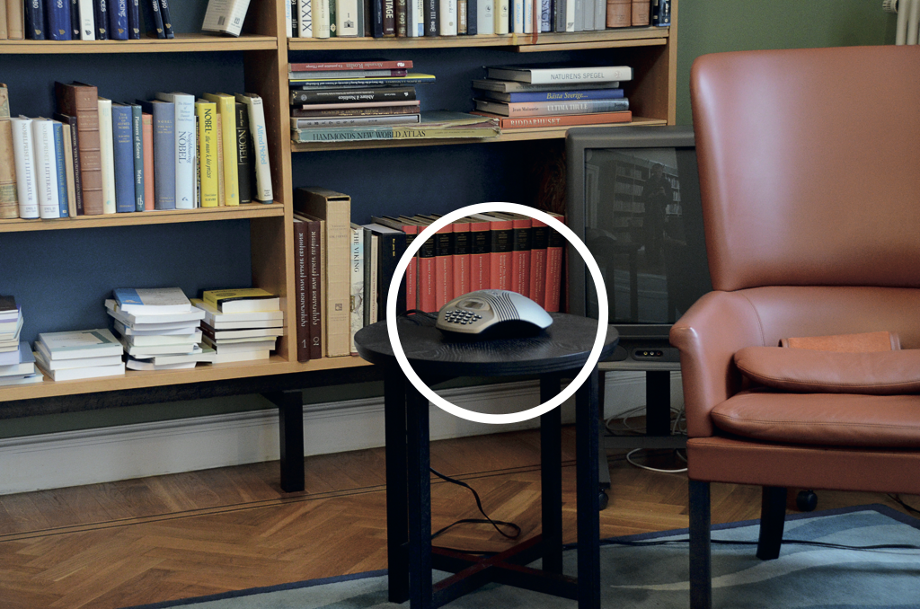
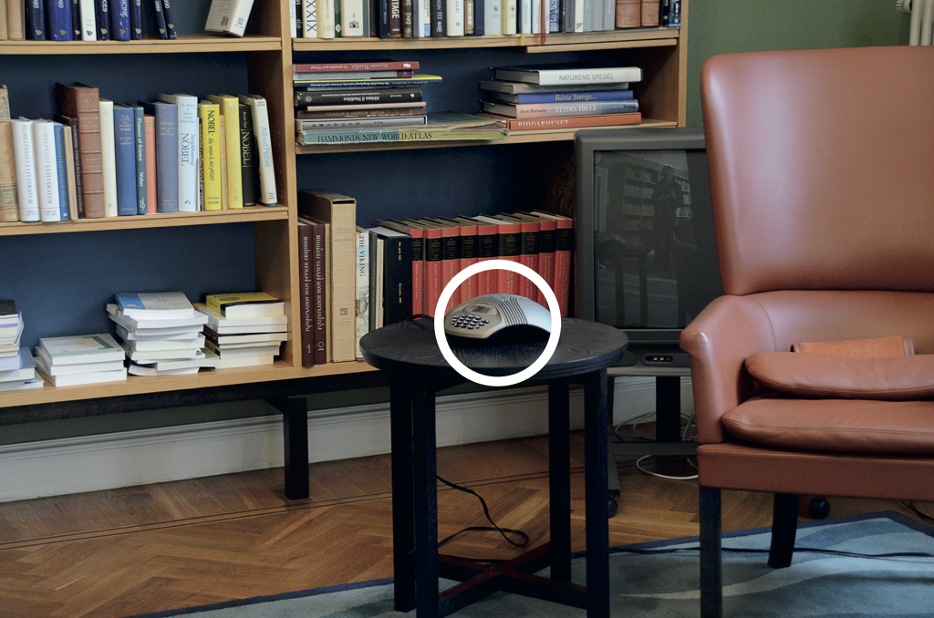
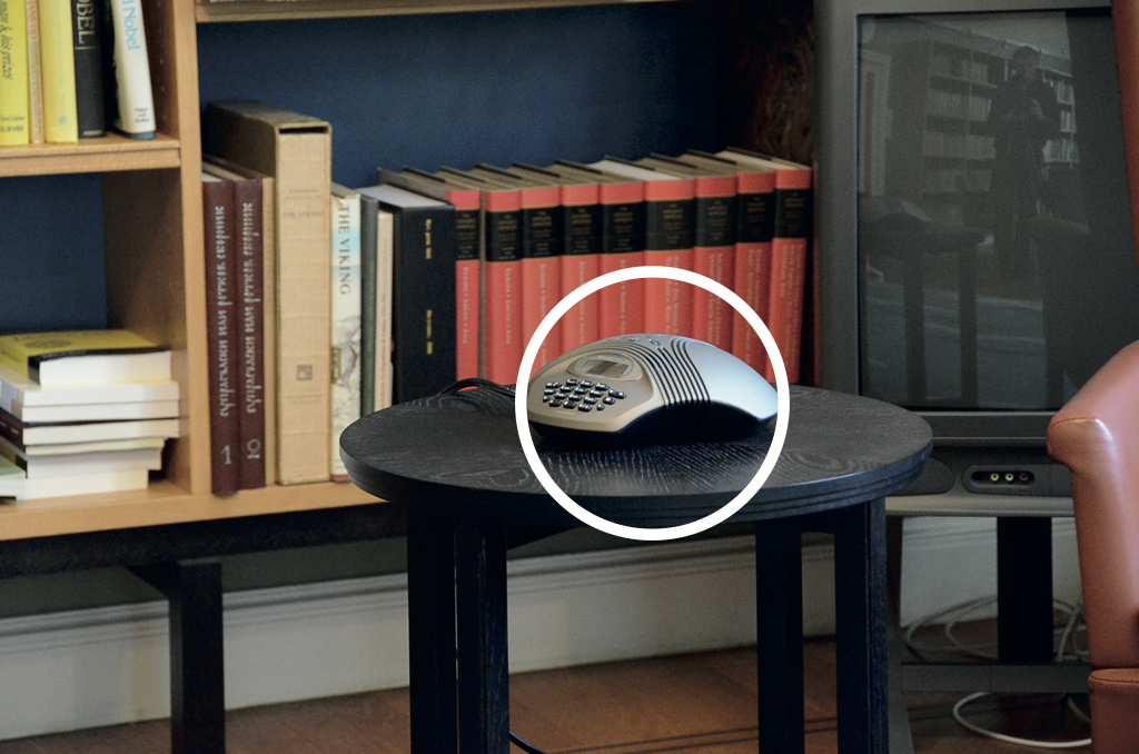
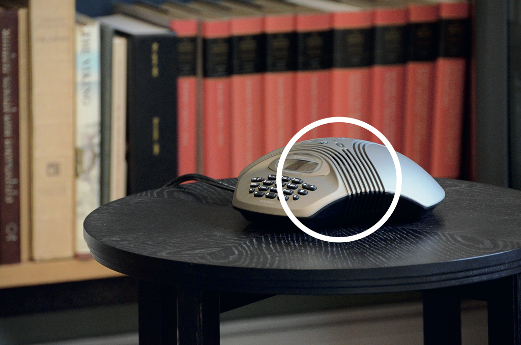
Figure 1: Illustration of the importance of having matching support regions of receptive fields when handling scaling transformations in the image domain. For this figure, we have simulated the effect of varying the distance between the object and the camera by varying the amount of zoom for a zoom lens. The left column illustrates the effect of having a fixed receptive field size in the image domain, and how that fixed receptive field size affects the backprojected receptive fields in the world, if there are significant scale variations. In the right column, the receptive field sizes are matched under the scaling transformation, as enabled by scale covariant receptive field families and scale channel networks, which makes it possible to define deep networks that are invariant to scaling transformations, which in turn enables scale generalization.

3 Scale generalization based on scale covariant and scale invariant receptive fields

A conceptual problem that we are interested in addressing is to be able to perform scale generalization, i.e., being able to train a deep network for image structures at some scale(s), and then being able to test the network at other scales, with maintained high recognition accuracy, and without complementary use of data augmentation.

The motivation for addressing this problem is that scale variations are very common in real-world image data, because of objects being of different sizes in the world, and because of variations in the viewing distance to the camera. Regular CNNs are, however, known to perform very poorly when exposed to testing data at scales that are not spanned by the training data.

Thus, a main goal of this work is to equip deep networks with prior knowledge to handle scaling transformations in image data, and specifically the ability to generalize to new scales that are not spanned by the training data.

The methodology that we will follow to achieve such scale generalization is to require that the image descriptors or the receptive fields in the deep network are to be truly scale covariant and scale invariant. The underlying idea is that the output from the image processing operations in the deep network should thus remain sufficiently similar under scaling transformations, as will be later formalized into the commutative diagram in Figure 2. Operationalized, we will require that the receptive field responses can be matched under scaling transformations. Specifically, we may require that the support regions of the receptive fields can be matched under scaling transformations.

Figure 1 illustrates these effects for scaling transformations in an indoor scene, caused by varying the amount of zoom for a zoom lens, which leads to similar scaling transformations as when varying the distance between the object and the camera. In the left column, we have marked receptive fields of constant size. Then, because of the scaling transformations, the backprojections of these receptive fields will be different in the world because of the scaling transformation, which may cause problems for a deep network, depending on how it is constructed. In the right column, the support regions follow the scaling transformations in a matched and scale covariant way, making it much easier for a deep network to recognize the object of interest under scaling transformations.

3.1 Scale covariance and scale invariance

With the scaling operator ${\cal S}_{s}$ defined by

$$({\cal S}_{s}f)(x)=f(S_{s}^{-1}x)=f(\tfrac{x}{s}).$$ (1)

and with $\Gamma$ denoting a family of feature map operators, the notion of scale covariance means that the feature maps should commute with scaling transformations and transform according to

$$\Gamma^{\prime}({\cal S}_{s}f)={\cal S}_{s}(\Gamma(f)),$$ (2)

where $\Gamma^{\prime}$ represents some possibly transformed feature map operator within the same family $\Gamma$, and adapted to the rescaled image domain. If we parameterize the feature map operator $\Gamma$ by a scale parameter $s$, we can make a commutative diagram as shown in Figure 2.

$$\begin{CD}(\Gamma_{s}f)(x)@>{\footnotesize s^{\prime}=Ss,\,\Gamma_{s}(f)(x)=\Gamma_{s^{\prime}}(f^{\prime})(x^{\prime})}>{}>(\Gamma_{s^{\prime}}f^{\prime})(x^{\prime})\\ \Big{\uparrow}\vbox{\hbox to0.0pt{$\scriptstyle{{\Gamma_{s}}}$\hss}}&&\Big{\uparrow}\vbox{\hbox to0.0pt{$\scriptstyle{{\Gamma_{s^{\prime}}}}$\hss}}\\ f(x)@>{\footnotesize\footnotesize x^{\prime}=Sx,\,f^{\prime}(x^{\prime})=f(x)}>{}>f^{\prime}(x^{\prime})\end{CD}$$

Figure 2: Commutative diagram for a scale-parameterized feature map operator $\Gamma_{s}$ that is applied to image data under scaling transformations. The commutative diagram, which should be read from the lower left corner to the upper right corner, means that irrespective of whether the input image is first subject to a scaling transformation and then the computation of a feature map, or whether the feature map is computed first and then transformed by a scaling transformation, we should get the same result. Note, however, that this definition of scale covariance assumes a multi-scale representation of the image data, and that direct availability to the image representations at the matching scale levels $s^{\prime}=Ss$ is necessary to complete the commutative diagram.

Implicit in Figure 2 is the notion that the deep network performs processing at multiple scales. The motivation for such a multi-scale approach is that for a vision system that observes an a priori unknown scene, there is no way to know in advance what scale is appropriate for processing the image data. In the absense of further information about what scales are appropriate, the only reasonable approach is to consider image representations at multiple scales. This motivation is similar to a corresponding motivation underlying scale-space theory Iij62 ; Wit83 ; Koe84 ; BWBD86-PAMI ; KoeDoo92-PAMI ; Lin93-Dis ; Lin94-SI ; Flo97-book ; WeiIshImi99-JMIV ; Haa04-book ; DuiFloGraRom04-JMIV ; Lin10-JMIV ; Lin13-ImPhys , which has developed a systematic approach for handling scaling transformations and image structures at multiple scales for hand-crafted image operations. Regarding deep networks that are to learn their image representations from image data, we proceed in a conceptually similar manner, by considering deep networks with multiple scale channels, that perform similar types of processing operations in all the scale channels, although over multiple scales.

Scale invariance does in turn mean that the final output from the deep network $\Lambda$, for example the result of max pooling or average pooling over the multiple scale channels, should not in any way be be affected by scaling transformations in the input

$$\Lambda({\cal S}_{s}f)=\Lambda(f),$$ (3)

at least over some predefined range of scale that defines the capacity of the system, where scale covariance of the receptive fields in the lower layers in the network makes scale invariance possible in the final layer(s).

3.2 Approach to scale generalization

By basing the deep network on image operations that are provably scale covariant and scale invariant, we can train on some scale(s) and test at other scale(s).

The scale covariant and scale invariant properties of the image operations will then allow for transfer between image information at different scales.

In the following, we will develop this approach for one specific class of deep networks. Conceptually similar approaches to scale generalization of deep networks are applied in (Lin20-JMIV, , Figures 15–16) and JanLin21-ICPR . Conceptually similar approaches to scale invariance and scale generalization for hand-crafted computer vision operations are applied in Lin97-IJCV ; Lin98-IJCV ; BL97-CVIU ; ChoVerHalCro00-ECCV ; MikSch04-IJCV ; Low04-IJCV ; BayEssTuyGoo08-CVIU ; TuyMik08-Book ; Lin15-JMIV ; Lin13-PONE .

3.3 Influence of the inner and the outer scales of the image

Before starting with the technical treatment, let us, however, remark that when designing scale-covariant and scale-invariant image processing operations, for a given discrete image there will be only a finite range of scales over which sufficiently good approximations to continuous scale covariance and scale invariant properties can be expected hold.

For a discrete image of finite resolution, there may at finer scales be interference with the inner scale of the image, given by the resolution of the sampling grid. For example, for the set of gradually zoomed images in Figure 1, the surface texture is clearly visible to the observer in the most zoomed-in image, whereas the same surface structure is far less visible to the observer in the most zoomed-out image. Correspondingly, if we would zoom in further to the telephone in the center of the image, peripheral parts of it may fall outside the image domain, corresponding to interference with the outer scale of the image, given by the image size. Sufficiently good numerical approximations to scale covariance and scale invariance can therefore only be expected to hold over a subrange of the scale interval for which the relevant scales of the interesting image structures are sufficiently within the range of scales defined by the inner and the outer scale of the image.

In the experiments to be presented in this work, we will handle these issues by a manual choice of the scale range for scale-space analysis as determined by properties of the dataset. When designing a computer vision system to analyze complex scenes with a priori unknown scales in the image data, there may, however, in addition be useful to add complementary mechanisms to handle the fact that an object seen from a far distance may contain far less fine-scale image structures than the same object seen from a nearby distance by the same camera. This implies that the recognition mechanisms in the system may need the ability to handle both the presence and the absense of image information over different subranges of scale, which goes beyond the continuous notions of scale covariance and scale invariance studied in this work. In a similar way, some mechanism may be needed to handle problems caused by the full object not being visible within the image domain or with a sufficient margin around its boundaries to reduce boundary effects of the spatially extended scale-space filters. For the purpose of the presentation in this paper, we will, however, leave automated handling of these issues for future work.

4 Gaussian derivative networks

In a traditional deep network, the filter weights are usually free variables with few additional constraints. In scale-space theory, on the other hand, theoretical results have been presented showing that Gaussian kernels and their corresponding Gaussian derivatives constitute a canonical class of image operations Iij62 ; Wit83 ; Koe84 ; BWBD86-PAMI ; KoeDoo92-PAMI ; Lin93-Dis ; Lin94-SI ; Flo97-book ; WeiIshImi99-JMIV ; Haa04-book ; Lin10-JMIV . In classical computer vision based on hand-crafted image features, it has been demonstrated that a large number of visual tasks can be successfully addressed by computing image features and image descriptors based on Gaussian derivatives, or approximations thereof, as the first layer of image features Lin97-IJCV ; Lin98-IJCV ; SchCro00-IJCV ; MikSch04-IJCV ; Low04-IJCV ; BayEssTuyGoo08-CVIU ; Lin15-JMIV . One could therefore raise the question if such Gaussian derivatives could also be used as computational primitives for constructing deep networks.

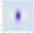
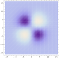
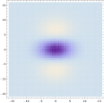
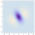
Figure 3: The 2-D Gaussian kernel with its Cartesian partial derivatives up to order two for $\sigma=4$.

Figure 4: First- and second-order directional derivatives of the 2-D Gaussian kernel computed from linear combinations of Cartesian partial derivatives according to equations (7) and (8) for $\sigma=4$ and $\varphi=\pi/6$.

4.1 Gaussian derivative layers

Motivated by the fact that a large number of visual tasks have been successfully addressed by first- and second-order Gaussian derivatives, which are the primitive filters in the Gaussian 2-jet, let us explore the consequences of using linear combinations of first- and second-order Gaussian derivatives as the class of possible filter weight primitives in a deep network. Thus, given an image $f$, which could either be the input image to the deep net, or some higher layer $F_{k}$ in the deep network, we first compute its scale-space representation by smoothing with the Gaussian kernel

$$L(x,y;\;\sigma)=(g(\cdot,\cdot;\;\sigma)*f(\cdot,\cdot))(x,y),$$ (4)

where

$$g(x,y;\;\sigma)=\frac{1}{2\pi\sigma^{2}}e^{-(x^{2}+y^{2})/2\sigma^{2}}.$$ (5)

Then, for simplicity with the notation for the spatial coordinates $(x,y)$ and the scale parameter $\sigma\in{\mathbb{R}}_{+}$ suppressed, we consider arbitrary linear combinations of first- and second-order Gaussian derivatives as the class of possible linear filtering operations on $f$ (or correspondingly for $F_{k}$):

$$J_{2,\sigma}(f)=C_{0}+C_{x}\,L_{\xi}+C_{y}\,L_{\eta}\\ +\frac{1}{2}(C_{xx}\,L_{\xi\xi}+2C_{xy}\,L_{\xi\eta}+C_{yy}\,L_{\eta\eta}),$$ (6)

where $L_{\xi}$, $L_{\eta}$, $L_{\xi\xi}$, $L_{\xi\eta}$ and $L_{\eta\eta}$ are first- and second-order scale-normalized derivatives Lin97-IJCV according to $L_{\xi}=\sigma\,L_{x}$, $L_{\eta}=\sigma\,L_{y}$, $L_{\xi\xi}=\sigma^{2}\,L_{xx}$, $L_{\xi\eta}=\sigma^{2}\,L_{xy}$ and $L_{\eta\eta}=\sigma^{2}\,L_{yy}$ (see Figure 4 for an illustration of Gaussian derivative kernels) and we have also added an offset term $C_{0}$ for later use in connection with non-linearities between adjacent layers.

Based on the notion that the set of Gaussian derivatives up to order $N$ is referred to as the Gaussian $N$-jet, we will refer to the expression (6), which is to be used as computational primitives for Gaussian derivative layers, as the linearily combined Gaussian 2-jet.

Since directional derivatives can be computed as linear combinations of partial derivatives, for first- and second-order derivatives we have (see Figure 4 for an illustration)

$$\begin{split}L_{\varphi}=\cos\varphi\,L_{x}+\sin\varphi\,L_{y},\end{split}$$ (7)

$$\begin{split}L_{\varphi\varphi}=\cos^{2}\varphi\,L_{xx}+2\cos\varphi\,\sin\varphi\,L_{xy}+\sin^{2}\varphi\,L_{yy},\end{split}$$ (8)

it follows that the parameterized second-order kernels of the form (6) span all possible linear combinations of first- and second-order directional derivatives.

The corresponding affine extension of such receptive fields, by replacing the rotationally symmetric Gaussian kernel (5) for scale-space smoothing by a corresponding affine Gaussian kernel, does also constitute a good idealized model for the receptive fields of simple cells in the primary visual cortex Lin13-BICY ; Lin21-Heliyon . In this treatment, we will, however, for simplicity restrict ourselves to regular Gaussian derivatives, based on partial derivatives and directional derivatives of rotationally symmetric Gaussian kernels.

In contrast to previous work in computer vision or functional modelling of biological visual receptive fields, where Gaussian derivatives are used as a first layer of linear receptive fields, we will, however, here investigate the consequences of coupling such receptive fields in cascade to form deep hierarchical image representations.

4.2 Definition of a Gaussian derivative network

To model Gaussian derivative networks with multiple feature channels in each layer, let us assume that the input image $f$ consists of $N_{0}$ image channels, for example with $N_{0}=1$ for a grey-level image or $N_{0}=3$ for a colour image. Assuming that each layer in the network $k\in[1,K]$ should consist of $N_{k}\in{\mathbb{Z}}_{+}$ parallel feature channels, the feature channel $F_{1}^{c_{out}}$ with feature channel index $c_{out}\in[1,N_{1}]$ in the first layer is given by

$$F_{1}^{c_{out}}(x,y;\;\sigma_{1})=\sum_{c_{in}\in[1,N_{0}]}J_{2,\sigma_{1}}^{1,c_{out},c_{in}}(f^{c_{in}}(\cdot,\cdot))(x,y;\;\sigma_{1}),$$ (9)

where $J_{2,\sigma_{1}}^{1,c_{out},c_{in}}$ is the linearily combined Gaussian 2-jet according to (6) at scale $\sigma_{1}$ that represents the contribution from the image channel with index $c_{in}$ in the input image $f$ to the feature channel with feature channel index $c_{out}$ in the first layer and $\sigma_{1}$ is the scale parameter in the first layer. The transformation between adjacent layers $k$ and $k+1$ is then for $k\geq 1$ given by

$$F_{k+1}^{c_{out}}(x,y;\;\sigma_{k+1})=\\ \sum_{c_{in}\in[1,N_{k}]}J_{2,\sigma_{k+1}}^{k+1,c_{out},c_{in}}(\theta_{k}^{c_{in}}(F_{k}^{c_{in}}(\cdot,\cdot;\;\sigma_{k})))(x,y;\;\sigma_{k+1}),$$ (10)

where $J_{2,\sigma_{k+1}}^{k+1,c_{out},c_{in}}$ is the linearily combined Gaussian 2-jet according to (6) that represents the contribution to the output feature channel $F_{k+1}^{c_{out}}$ with feature channel index $c_{out}\in[1,N_{k+1}]$ in layer $k+1$ from the input feature channel $F_{k}^{c_{in}}$ with feature channel index $c_{in}\in[1,N_{k}]$ in layer $k$ and $\theta_{k}^{c_{in}}$ represents some non-linearity, such as a ReLU stage. The parameter $\sigma_{k+1}$ is the scale parameter for computing layer $k+1$ and the parameter $\sigma_{k}$ is the scale parameter for computing layer $k$.

Of course, the parameters $C_{0}$, $C_{x}$, $C_{y}$, $C_{xx}$, $C_{xy}$ and $C_{yy}$ in the linearily combined Gaussian 2-jet according to (6) should be allowed to be learnt differently for each layer $k\in[1,K]$ and for each combination of input channel $c_{in}$ and output channel $c_{out}$. Written out with explicit index notation for the layers and the input and output feature channels for these parameters, the explicit expression for $J_{2,\sigma_{k}}^{k,c_{out},c_{in}}$ in (9) and (10) is given by

$$\begin{split}J_{2,\sigma_{k}}^{k,c_{out},c_{in}}(h^{c_{in}})=\end{split}$$

$$\begin{split}=C_{0}^{k,c_{out},c_{in}}+C_{x}^{k,c_{out},c_{in}}\,\sigma_{k}\,L_{x}+C_{y}^{k,c_{out},c_{in}}\,\sigma_{k}\,L_{y}+\end{split}$$

$$\begin{split}+\frac{1}{2}(C_{xx}^{k,c_{out},c_{in}}\,\sigma_{k}^{2}\,L_{xx}+2C_{xy}^{k,c_{out},c_{in}}\,\sigma_{k}^{2}\,L_{xy}+\end{split}$$

$$\begin{split}\hphantom{+\frac{1}{2}(}+C_{yy}^{k,c_{out},c_{in}}\,\sigma_{k}^{2}\,L_{yy}),\end{split}$$ (11)

with $L_{x}$, $L_{y}$, $L_{xx}$, $L_{xy}$ and $L_{yy}$ here denoting the partial derivatives of the scale-space representation obtained by convolving the argument $h^{c_{in}}$ with a Gaussian kernel (5) with standard deviation $\sigma_{k}$ according to (4)

$$L_{x^{\alpha}y^{\beta}}=\partial_{x^{\alpha}y^{\beta}}\left(g(\cdot,\cdot;\;\sigma_{k})*h^{c_{in}}(\cdot,\cdot)\right),$$ (12)

and with $h^{c_{in}}$ representing the image or feature channel with index $c_{in}$ in either the input image $f$ or some higher feature layer $F_{k-1}$.

When coupling several combined smoothing and differentiation stages in cascade in this way, with pointwise non-linearities in between, it is natural to let the scale parameter for layer $k$ be proportional to an initial scale level $\sigma_{0}$, such that the scale parameter $\sigma_{k}$ in layer $k$ is $\sigma_{k}=\beta_{k}\,\sigma_{0}$ for some set of $\beta_{k}\geq\beta_{k-1}\geq 1$ and some minimum scale level $\sigma_{0}>0$. Specifically, it is natural to choose the relative factors for the scale parameters according to a geometric distribution

$$\sigma_{k}=r^{k-1}\,\sigma_{0}$$ (13)

for some $r\geq 1$. By gradually increasing the size of the receptive fields in this way, the transition from lower to higher layers in the hierarchy will correspond to gradual transitions from local to regional information. For continuous networks models, this mechanism thus provides a way to gradually increase the receptive field size in deeper layers without explicit need for a discrete subsampling operation that would imply larger steps in the receptive fields size of deeper layers.

By additionally varying the parameter $\sigma_{0}$ in the above relationship, either continuously with $\sigma_{0}\in{\mathbb{R}}$ or according to some self-similar distribution

$$\sigma_{0}=\gamma^{i}$$ (14)

for some set of integers $i\in{\mathbb{Z}}$ and some $\gamma>1$, the Gaussian derivative network defined from (9) and (10) will constitute a multi-scale representation that will also be provably scale covariant, as will be formally shown below in Section 4.3. Specifically, the network obtained for each value of $\sigma_{0}$, with the derived values of $\sigma_{1}$ in (9) as well as of $\sigma_{k}$ and $\sigma_{k+1}$ in (10), will be referred to as a scale channel. Letting the initial scale levels be given by a self-similar distribution in this way reflects the desire that in the absense of further information the deep network should be agnostic with regard to preferred scales in the input.

A similar idea of using Gaussian derivatives as structured receptive fields in convolutional networks has also been explored in JacGemLouSme16-CVPR , although not in the relation to scale covariance, multiple scale channels or using a self-similar sampling of the scale levels at consecutive depths.

$$\hskip 17.07164pt\begin{CD}F_{k}@>{F^{\prime}_{k}(x^{\prime},y^{\prime};\;\sigma^{\prime})=F_{k}(x,y;\;\sigma)}>{}>F_{k}^{\prime}\\ @A{{\cal J}_{2,\sigma_{k}}}A{}A@A{}A{{\cal J}_{k,\sigma^{\prime}_{k}}}A\\ \vdots\vdots\\ @A{{\cal J}_{2,\sigma_{3}}}A{}A@A{}A{{\cal J}_{2,\sigma^{\prime}_{3}}}A\\ F_{2}@>{F^{\prime}_{2}(x^{\prime},y^{\prime};\;\sigma^{\prime})=F_{2}(x,y;\;\sigma)}>{}>F_{2}^{\prime}\\ @A{{\cal J}_{2,\sigma_{2}}}A{}A@A{}A{{\cal J}_{2,\sigma^{\prime}_{2}}}A\\ F_{1}@>{F^{\prime}_{1}(x^{\prime},y^{\prime};\;\sigma^{\prime})=F_{1}(x,y;\;\sigma)}>{}>F_{1}^{\prime}\\ @A{{\cal J}_{2,\sigma_{1}}}A{}A@A{}A{{\cal J}_{2,\sigma^{\prime}_{1}}}A\\ f@>{x^{\prime}=Sx,\,y^{\prime}=Sx,\,\sigma^{\prime}=S\sigma}>{}>f^{\prime}\end{CD}$$

Figure 5: Commutative diagram for a scale-covariant Gaussian derivative network constructed by coupling linear combinations of scale-normalized Gaussian derivatives in cascade, with non-linear ReLU stages in between. Because of the transformation properties of the individual layers under scaling transformations, it will be possible to perfectly match the corresponding layers $F_{k}$ and $F_{k}^{\prime}$ under a scaling transformation of the underlying image domain $f^{\prime}(x^{\prime})=f(x)$ for $x^{\prime}=Sx$ and $y^{\prime}=Sy$, provided that the scale parameter $\sigma_{k}$ in layer $k$ is proportional to the scale parameter $\sigma_{1}$ in the first layer, $\sigma_{k}=r_{k}^{2}\,\sigma_{1}$, for some scalar constant $r_{k}>1$. For such a network, the scale parameters in the two domains should be related according to $\sigma_{k}^{\prime}=S\sigma_{k}$. Note, however, that for a scale-discretized implementation, this commutative property holds exactly over a continuous image domain only if the scale levels $\sigma$ and $\sigma^{\prime}$ are part of the scale grid, thus specifically only for discrete scaling factors $S$ that can be exactly represented on the discrete scale grid. For other scaling factors, the results will instead be numerical approximations, with the accuracy of the approximation determined by a the combination of the network architecture with the learning algorithm. (In this schematic illustration, we have for simplicity suppressed the notation for multiple feature channels in the different layers, and also suppressed the notation for the pointwise non-linearities between adjacent layers.)

4.3 Provable scale covariance

To prove that a deep network constructed by coupling linear filtering operations of the form (6) with pointwise non-linearities in between is scale covariant, let us consider two images $f$ and $f^{\prime}$ that are related by a scaling transformation $f^{\prime}(x^{\prime},y^{\prime})=f(x,y)$ for $x^{\prime}=S\,x$, $y^{\prime}=S\,y$ and some spatial scaling factor $S>0$.

A basic scale covariance property of the Gaussian scale-space representation is that if the scale parameters $\sigma$ and $\sigma^{\prime}$ in the two image domains are related according to $\sigma^{\prime}=S\,\sigma$, then the Gaussian scale-space representations are equal at matching image points and scales (Lin97-IJCV, , Eq. (16))

$$L^{\prime}(x^{\prime},y^{\prime};\;\sigma^{\prime})=L(x,y;\;\sigma).$$ (15)

Additionally regarding spatial derivatives, it follows from a general result in (Lin97-IJCV, , Eq. (20)) that the scale-normalized spatial derivatives will also be equal (when using scale normalization power $\gamma=1$ in the scale-normalized derivative concept):

$$L^{\prime}_{\xi^{\alpha}\eta^{\beta}}(x^{\prime},y^{\prime};\;\sigma^{\prime})=L_{\xi^{\alpha}\eta^{\beta}}(x,y;\;\sigma).$$ (16)

Applied to the linearily combined Gaussian 2-jet in (6), it follows that also the linearily combined Gaussian 2-jets computed from two mutually rescaled scalar image patterns $f$ and $f^{\prime}$ will be related by a similar scaling transformation

$$J_{2,\sigma^{\prime}}(f^{\prime}(\cdot,\cdot))(x^{\prime},y^{\prime};\;\sigma^{\prime})=J_{2,\sigma}(f(\cdot,\cdot))(x,y;\;\sigma)$$ (17)

provided that the image positions $(x,y)$ and $(x^{\prime},y^{\prime})$ and the scale parameters $\sigma$ and $\sigma^{\prime}$ are appropriately matched, and that the parameters $C_{0}$, $C_{x}$, $C_{y}$, $C_{xx}$, $C_{xy}$ and $C_{yy}$ in (6) are shared between the two 2-jets at the different scales.

Thus, provided that the image positions and the scale levels are appropriately matched according to $x^{\prime}=S\,x$, $y^{\prime}=S\,y$ and $\sigma^{\prime}=S\,\sigma$, it holds that the corresponding feature channels $F_{1}^{c_{out}}$ and ${F^{\prime}}_{1}^{c_{out}}$ in the first layer according to (9) are equal up to a scaling transformation:

$$\begin{split}{F^{\prime}}_{1}^{c_{out}}(x^{\prime},y^{\prime};\;\sigma^{\prime}_{1})\end{split}$$

$$\begin{split}=\sum_{c_{in}\in[1,N_{0}]}J_{2,\sigma^{\prime}_{1}}^{1,c_{out},c_{in}}({f^{\prime}}^{c_{in}}(\cdot,\cdot))(x^{\prime},y^{\prime};\;\sigma^{\prime}_{1})=\\ \end{split}$$

$$\begin{split}=\sum_{c_{in}\in[1,N_{0}]}J_{2,\sigma_{1}}^{1,c_{out},c_{in}}(f^{c_{in}}(\cdot,\cdot))(x,y;\;\sigma_{1})\end{split}$$

$$\begin{split}=F_{1}^{c_{out}}(x,y;\;\sigma_{1}),\end{split}$$ (18)

provided that the parameters $C_{0}^{1,c_{out},c_{in}}$, $C_{x}^{1,c_{out},c_{in}}$,
$C_{y}^{1,c_{out},c_{in}}$, $C_{xx}^{1,c_{out},c_{in}}$, $C_{xy}^{1,c_{out},c_{in}}$ and $C_{yy}^{1,c_{out},c_{in}}$ in the 2-jets according to (11) for $k=1$ are shared between the scale channels for corresponding combinations of feature channels, as indexed by $c_{in}$ and $c_{out}$.

By continuing a corresponding construction of higher layers, by applying similar operations in cascade, with pointwise non-linearities such as ReLU stages in between, according to (10) with the initial scale levels $\sigma_{0}$ and $\sigma_{0}^{\prime}$ in (13) related according to $\sigma_{0}^{\prime}=S\,\sigma_{0}$, it follows that also the corresponding feature channels ${F^{\prime}}_{k+1}^{c_{out}}$ and $F_{k+1}^{c_{out}}$ in the higher layers in the hierarchy will be equal up to a scaling transformation, since the input data from the adjacent finer layers ${F^{\prime}}_{k}^{c_{in}}$ and $F_{k}^{c_{in}}$ are already known to be related by plain scaling transformation (see Figure 5 for an illustration):

$$\begin{split}{F^{\prime}}_{k+1}^{c_{out}}(x^{\prime},y^{\prime};\;\sigma^{\prime}_{k+1})\end{split}$$

$$\begin{split}=\sum_{c_{in}\in[1,N_{k}]}J_{2,\sigma^{\prime}_{k+1}}^{k+1,c_{out},c_{in}}(\theta_{k}^{c_{in}}({F^{\prime}}_{k}^{c_{in}}(\cdot,\cdot;\;\sigma^{\prime}_{k})))(x^{\prime},y^{\prime};\;\sigma^{\prime}_{k+1})\end{split}$$

$$\begin{split}=\sum_{c_{in}\in[1,N_{k}]}J_{2,\sigma_{k+1}}^{k+1,c_{out},c_{in}}(\theta_{k}^{c_{in}}(F_{k}^{c_{in}}(\cdot,\cdot;\;\sigma_{k})))(x,y;\;\sigma_{k+1})\end{split}$$

$$\begin{split}=F_{k+1}^{c_{out}}(x,y;\;\sigma_{k+1}),\end{split}$$ (19)

again assuming that the parameters $C_{0}^{k,c_{out},c_{in}}$, $C_{x}^{k,c_{out},c_{in}}$, $C_{y}^{k,c_{out},c_{in}}$, $C_{xx}^{k,c_{out},c_{in}}$, $C_{xy}^{k,c_{out},c_{in}}$ and $C_{yy}^{k,c_{out},c_{in}}$ in the 2-jets according to (11) are shared between the scale channels for corresponding layers and combinations of feature channels, as indexed by $c_{in}$ and $c_{out}$.

A pointwise non-linearity, such as a ReLU stage, trivially commutes with scaling transformations and does therefore not affect the scale covariance properties.

In a recursive manner, we thereby prove that scale covariance in the lower layers imply scale covariance in any higher layer.

4.4 Provable scale invariance

To prove scale invariance after max pooling over the scale channels, let us assume that we have an infinite set of scale channels ${\cal S}$, with the initial scale values $\sigma_{0}$ in (14) either continuously distributed with

$${\cal S}=\{\sigma\in{\mathbb{R}}_{+}\}$$ (20)

or discrete in the set

$${\cal S}=\{\sigma_{i}=\gamma^{i},\forall i\in{\mathbb{Z}}\}.$$ (21)

for some $\gamma>1$.

The max pooling operation over the scale channels for feature channel $c$ in layer $k$ will then at every image position $(x,y)$ and with the scale parameter in this layer $\sigma_{k}$ and the relative scale factor $r$ according to (13) return the value

$$F_{k,sup}^{c}(x,y)=\sup_{\sigma_{k}}F_{k}^{c}(x,y;\;\sigma_{k})=\sup_{\sigma_{0}\in{\cal S}}F_{k}^{c}(x,y;\;r^{k-1}\sigma_{0}).$$ (22)

Let us without essential loss of generality assume that the scaling transformation is performed around the image point $(x,y)$, implying that we can without essential loss of generality assume that the origin is located at this point. The set of feature values before the scaling transformation is then given by

$$M=\{F_{k}^{c}(0,0;\;r^{k-1}\sigma_{0})\,\forall\sigma_{0}\}$$ (23)

and the set of feature values after the scaling transformation

$$M^{\prime}=\{{F^{\prime}}^{c}_{k}(0,0;\;r^{k-1}\sigma_{0}^{\prime})\,\forall\sigma_{0}^{\prime}\}.$$ (24)

With the relationship $\sigma_{0}^{\prime}=S\,\sigma_{0}$, these sets are clearly equal provided that $S>0$ in the continuous case or $S=\gamma^{j}$ for some $j\in{\mathbb{Z}}$ in the discrete case, implying that the supremum of the set is preserved (or the result of any other permutation invariant pooling operation, such as the average). Because of the closedness property under scaling transformations, the scaling transformation just shifts the set of feature values over scales along the scale axis.

In this way, the result after max pooling over the scale channels is essentially scale invariant, in the sense that the result of the max pooling operation at any image point follows the geometric transformation of the image point under scaling transformations.

When using a finite number of scale channels, the result of max pooling over the scale channels is, however, not guaranteed to truly scale invariant, since there could be boundary effects, implying that the maximum over scales moves in to or out from a finite scale interval, because of the scaling transformation that shifts the position of the scale maxima on the scale axis.

To reduce the likelihood of such effects occurring, we propose as design criterion to ensure that there should be a sufficient number of additional scale channels below and above the effective training scales in the training data. The intention behind this is that the learning algorithm could then learn that the image structures that occur below and above the effective training scales are less relevant, and thereby associate lower values of the feature maps to such image structures. In this way, the risk should be reduced that erroneous types of image structures are being picked up by the max pooling operation over the multiple scale channels, by the scale channels near the scale boundaries thereby having lower magnitude values in their feature maps than the central ones.

A similar scale boundary handling strategy is used in the scale channel networks based on applying a fixed CNN to a set of rescalings of the original image in JanLin21-ICPR , as opposed to the approach here based on applying a set of rescaled CNNs to a fixed size input image.

5 Experiments with a single-scale-channel network

To investigate the ability of these types of deep hierarchical Gaussian derivative networks to capture image structures with different image shapes, we first did initial experiments with the regular MNIST dataset LecBotBenHaf98-ProcIEEE . We constructed a 6-layer network in PyTorch PasGroChiChaYanDeVLinDesAntLer17-NIPS with 12-14-16-20-64 channels in the intermediate layers and 10 output channels, intended to learn each type of digit.

We chose the initial scale level $\sigma_{0}=0.9$ pixels and the relative scale ratio $r=1.25$ in (13), implying that the maximum value of $\sigma$ is $0.9\times 1.25^{5}\approx 2.7$ pixels relative to the image size of $28\times 28$ pixels. The individual receptive fields do then have larger spatial extent because of the spatial extent of the Gaussian kernels used for image smoothing and the larger positive and negative side lobes of the first- and second-order derivatives.

We used regular ReLU stages between the filtering steps, but no spatial max pooling or spatial stride, and no fully connected layer, since such operations would destroy the scale covariance. Instead, the receptive fields are solely determined from linear combinations of Gaussian derivatives, with successively larger receptive fields of size $\sigma_{0}\,r^{k-1}$, which enable a gradual integration from local to regional image structures. In the final layer, only the value at the central pixel is extracted, or here for an even image size, the average over the central $2\times 2$ neighbourhood, which, however, destroys full scale covariance. To ensure full scale covariance, the input images should instead have odd image size.

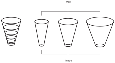
Figure 6: (left) Schematic illustration of the architecture of the single-scale-channel network, with 6 layers of receptive fields at successively coarser levels of scale. (right) Schematic illustration of the architecture of a multi-scale-channel network, with multiple parallel scale channels over a self-similar distribution of the initial scale level $\sigma_{0}$ in the hierarchy of Gaussian derivative layers coupled in cascade.

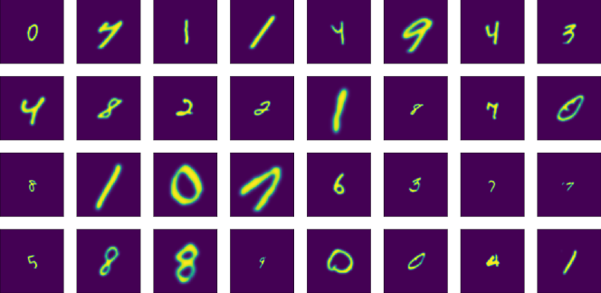
Figure 7: Sample images from the MNIST Large Scale dataset JanLin21-ICPR ; JanLin20-MNISTLargeScale . This figure shows digits for sizes in the range [1, 4], for which there are training data. In addition, the MNIST Large Scale dataset contains testing data over the wider size range [1/2, 8].

The network was trained on 50 000 of the training images in the dataset, with the offset term $C_{0}^{k,c_{out},c_{in}}$ that serves as the bias for the non-linearity and the weights $C_{x}^{k,c_{out},c_{in}}$, $C_{y}^{k,c_{out},c_{in}}$, $C_{xx}^{k,c_{out},c_{in}}$, $C_{xy}^{k,c_{out},c_{in}}$ and $C_{yy}^{k,c_{out},c_{in}}$ of the Gaussian derivatives in (11) initiated to random values and trained individually for each layer and feature channel by stochastic gradient descent over 40 epochs using the Adam optimizer KinBa15-ICLR set to minimize the binary cross-entropy loss. We used a cosine learning curve with maximum learning rate of 0.01 and minimum learning rate 0.00005 and using batch normalization over batches with 50 images. The experiment lead to 99.93 % training accuracy and 99.43 % test accuracy on the test dataset containing 10 000 images.

Notably, the training accuracy does not reach 100.00 %, probably because of the restricted shapes of the filter weights, as determined by the a priori shapes of the receptive fields in terms of linear combinations of first- and second-order Gaussian derivatives. Nevertheless, the test accuracy is quite good given the moderate number of parameters in the network ($6\times(12+12\times 14+14\times 16+16\times 20+20\times 64+64\times 10)=15~{}864$).

5.1 Discrete implementation

In the numerical implementation of scale-space smoothing, we used separable smoothing with the discrete analogue of the Gaussian kernel $T(n;\;s)=e^{-s}I_{n}(s)$ for $s=\sigma^{2}$ in terms of modified Bessel functions $I_{n}$ of integer order Lin90-PAMI . The discrete derivative approximations were computed by central differences, $\delta_{x}=(-1/2,0,1/2)$, $\delta_{xx}=(1,-2,1)$, $\delta_{xy}=\delta_{x}\delta_{y}$, etc., implying that the spatial smoothing operation can be shared between derivatives of different order, and implying that scale-space properties are preserved in the discrete implementation of the Gaussian derivatives Lin93-JMIV . This is a general methodology for computing Gaussian derivatives for a large number of visual tasks.

By computing the Gaussian derivative responses in this way, the scale-space smoothing is only performed once for each scale level, and there is no need for repeating the scale-space smoothing for each order of the Gaussian derivatives.

6 Experiments with a multi-scale-channel network

To investigate the ability of a multi-scale-channel network to handle spatial scaling transformations, we made experiments on the MNIST Large Scale dataset JanLin21-ICPR ; JanLin20-MNISTLargeScale . This dataset contains rescaled digits from the original MNIST dataset LecBotBenHaf98-ProcIEEE embedded in images of size $112\times 112$, see Figure 7 for an illustration.

For training, we used either of the datasets containing 50 000 rescaled digits with relative scale factors 1, 2 or 4, respectively, henceforth referred to as training sizes 1, 2 and 4. For testing, the dataset contains 10 000 rescaled digits with relative scale factors between 1/2 and 8, respectively, with a relative scale ratio of $\sqrt[4]{2}$ between adjacent testing sizes.

Scale generalization performance when training on size 1

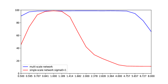
Scale generalization performance when training on size 2

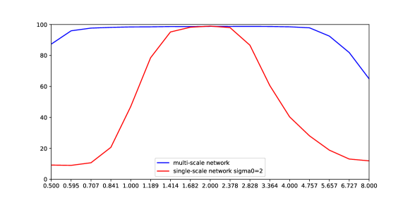
Scale generalization performance when training on size 4

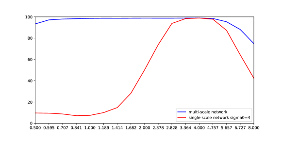
Figure 8: Experiments showing the ability of a multi-scale-channel network to generalize to new scale levels not present in the training data. In the top row, all training data are for size 1, whereas we evaluate on multiple testing sets for each one of the sizes between 1/2 and 8. The red curve shows the generalization performance for a single-scale-channel network for $\sigma_{0}=1$, whereas the blue curve shows the result for a multi-scale-channel network covering the range of $\sigma_{0}$-values between $1/\sqrt{2}$ and 8. As can be seen from the result, the generalization ability is much better for the multi-scale-channel network compared to the single-scale-channel network. In the middle row, a similar type of experiment is repeated for training size 2 and with $\sigma_{0}=2$ for the single-scale-channel network. In the bottom row, a similar experiment is performed for training size 4 and with $\sigma_{0}=4$ for the single-scale-channel network. (Horizontal axis: Scale of testing data.)

Scale generalization performance when training on different sizes: Default network

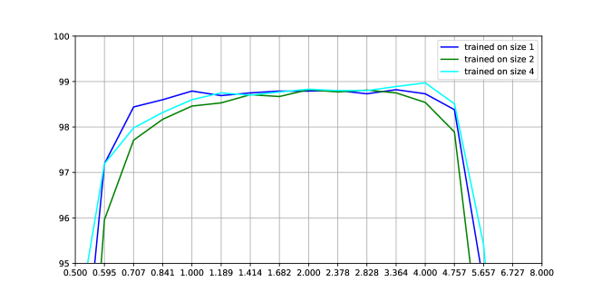
Scale generalization performance when training on different sizes: Larger network

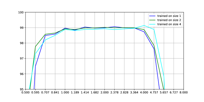
Figure 9: Joint visualization of the generalization performance when training a multi-scale-channel Gaussian derivative network on training data with sizes 1, 2 and 4, respectively. As can be seen from the graphs, the performance is rather similar for all these networks over the size range between 1 and 4, a range for which the discretization errors in the discrete implementation can be expected to be low (a problem at too fine scales) and the influence of boundary effects causing a mismatch between what parts of the digits are visible in the testing data compared to a training data (a problem at too coarse scales). The top figure shows the results for the default network with 12-16-24-32-64-10 feature channels. The bottom figure shows the results for a larger network with 16-24-32-48-64-10 feature channels. (Horizontal axis: Scale of testing data.)

To investigate the properties of a multi-scale-channel architecture experimentally, we created a multi-scale-channel network with 8 scale channels with their initial scale values $\sigma_{0}$ between $1/\sqrt{2}$ and 8 and a scale ratio of $\sqrt{2}$ between adjacent scale channels. For each channel, we used a Gaussian derivative network of similar architecture as the single-scale-channel network, with 12-14-16-20-64 channels in the intermediate layers and 10 output channels, and with a relative scale ratio $r=1.25$ (13) between adjacent layers, implying that the maximum value of $\sigma$ in each channel is $\sigma_{0}\times 1.25^{5}\approx 3.1~{}\sigma_{0}$ pixels.

Importantly, the parameters $C_{0}^{k,c_{out},c_{in}}$, $C_{x}^{k,c_{out},c_{in}}$, $C_{y}^{k,c_{out},c_{in}}$, $C_{xx}^{k,c_{out},c_{in}}$, $C_{xy}^{k,c_{out},c_{in}}$ and $C_{yy}^{k,c_{out},c_{in}}$ in (11) are shared between the scale channels, implying that the scale channels together are truly scale covariant, because of the parameterization of the receptive fields in terms of scale-normalized Gaussian derivatives. The batch normalization stage is also shared between the scale channels. The output from max pooling over the scale channels is furthermore truly scale invariant, if we assume an infinite number of scale channels, so that scale boundary effects can be disregarded.

Figure 8 shows the result of an experiment to investigate the ability of such a multi-scale-channel network to generalize to testing at scales not present in the training data.

For the experiment shown in the top figure, we have used 50 000 training images for training size 1, and 10 000 testing images for each one of the 19 testing sizes between 1/2 and 8 with a relative size ratio of $\sqrt[4]{2}$ between adjacent testing sizes. The red curve shows the generalization performance for a single-scale-channel network with $\sigma_{0}=1$, whereas the blue curve shows the generalization performance for the multi-scale-channel network with 8 scale channels between $1/\sqrt{2}$ and 8.

As can be seen from the graphs, the generalization performance is very good for the multi-scale-channel network, for sizes in roughly in the range $1/\sqrt{2}$ and $4\sqrt{2}$. For smaller testing sizes near 1/2, there are discretization problems due to sampling artefacts and too fine scale levels relative to the grid spacing in the image, implying that the transformation properties under scaling transformations of the underlying Gaussian derivatives are not well approximated in the discrete implementation. For larger testing sizes near 8, there are problems due to boundary effects and that the entire digit is not visible in the testing stage, implying a mismatch between the training data and the testing data. Otherwise, the generalization performance is very good over the size range between 1 and 4.

For the single-scale-channel network, the generalization performance to scales far from the scales in the training data is on the other hand very poor.

In the middle figure, we show the result of a similar experiment for training images of size 2 and with the initial scale level $\sigma_{0}=2$ for the single-scale-channel network. The bottom figure shows the result of a similar experiment performed with training images of size 4 and with the initial scale level $\sigma_{0}=4$ for the single-scale-channel network.

Selected scale levels: Larger network trained at size 1

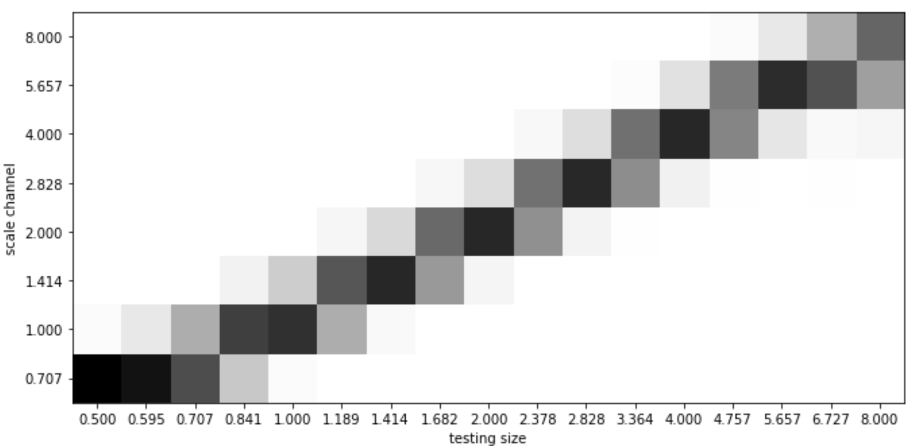
Selected scale levels: Larger network trained at size 2

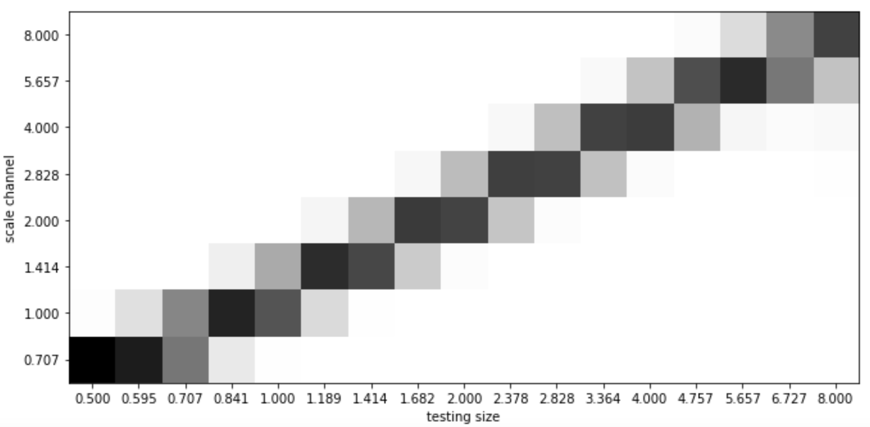
Selected scale levels: Larger network trained at size 4

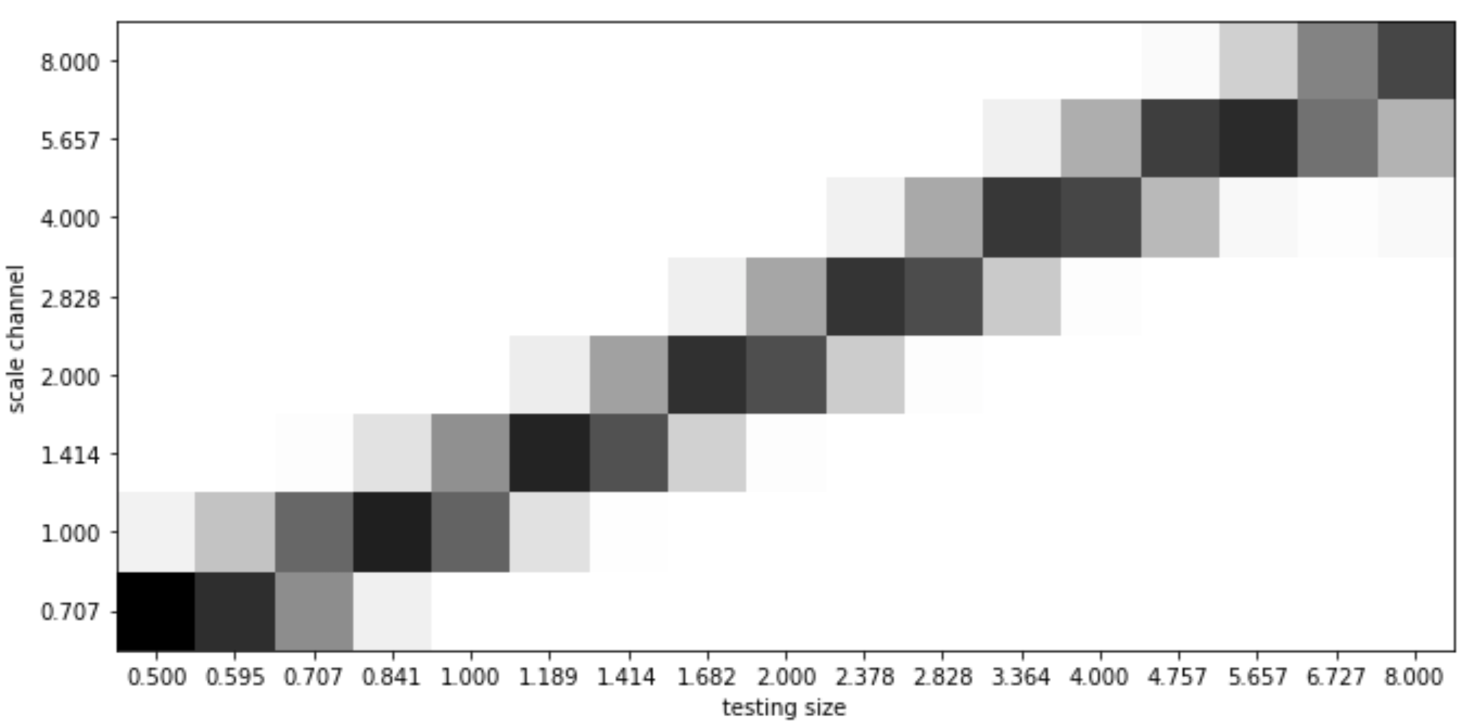
Figure 10: Visualization of the scale channels that are selected in the max pooling stage, when training the larger network for each one of the sizes 1, 2 and 4. For each testing size, shown on the horizontal axis, the vertical axis displays a histogram of the scale levels at which the maximum over the scale channels is assumed for the different samples in the testing set, with the lowest scale at the bottom and the highest scale at the top. As can be seen from the figure, there is a general tendency of the composed classification scheme to select coarser scale levels with increasing size of the image structures, in agreement with the conceptual similarity to classical methods for scale selection based on detecting local extrema over scales of scale-normalized derivatives, the difference being that here only the global maximum over scale is used, as opposed to the detection of multiple local extrema over scale in classical scale selection methods.

Figure 9 shows a joint visualization of the generalization performance for all these experiments, where we have also zoomed in on the top performance values in the range 98-99 %. In addition to the results from the default network with 12-16-24-32-64-10 feature channels, we do also show results obtained from a larger network with 16-24-32-48-64-10 feature channels, which has more degrees of freedom in the training stage (a total number of $6\times(16+16\times 24+24\times 32+32\times 48+48\times 64+64\times 10)=38~{}496$ parameters) and leads to higher top performance and also somewhat better generalization performance. As can be seen from the graphs, the performance values for training sizes 1, 2 and 4, respectively, are quite similar for testing data with sizes in the range between 1 and 4, a size range for which the discretization errors in the discrete implementation can be expected to be low (a problem at too fine scales) and the influence of boundary effects causing a mismatch between what parts of the digits are visible in the testing data compared to the training data (a problem at too coarse scales).

To conclude, the experiment demonstrates that it is possible to use the combination of (i) scale-space features as computational primitives for a deep learning method with (ii) the closed-form transformation properties of the scale-space primitives under scaling transformations to (iii) make a deep network generalize to new scale levels not spanned by the training data.

6.1 Scale selection properties

Since the Gaussian derivative network is expressed in terms of scale-normalized derivatives over multiple scales, and the max-pooling operation over the scale channels implies detecting maxima over scale, the resulting approach shares similarities to classical methods for scale selection based on local extrema over scales of scale-normalized derivatives Lin97-IJCV ; Lin98-IJCV ; Lin21-EncCompVis . The approach is also closely related to the scale selection approach in LooLiTax09-LNCS ; LiTaxLoo12-IVC based on choosing the scales at which a supervised classifier delivers class labels with the highest posterior.

A limitation of choosing only a single maximum over scales compared to processing multiple local extrema over scales as in Lin97-IJCV ; Lin98-IJCV ; Lin21-EncCompVis , however, is that the approach may be sensitive to boundary effects at the scale boundaries, implying that the scale generalization properties may be affected depending on how many coarser-scale and/or finer-scale channels are being processed relative to the scale of the image data.

In Figure 10, we have visualized the scale selection properties when applying these multi-scale-channel Gaussian derivative networks to the MNIST Large Scale dataset. For each one of the training sizes 1, 2 and 4, we show what scales are selected as function of the testing size. Specifically, for each testing size, shown on the horizontal axis, we display a histogram of the scale channels at which the maximum over scales is assumed over all the samples in the testing set, with the finest scale at the bottom and the coarsest scale at the top.

As can be seen from the figure, the network has an overall tendency of selecting coarser scale levels with increasing size of the image structures it is applied to. Specifically, the overall tendency is that the selected scale is proportional to the size of the testing data, in agreement with the theory for scale selection based on local extrema over scales of scale-normalized derivatives.

Except for minor quantization variations due to the discrete bins, these scale selection histograms are very similar for the different training sizes 1, 2 and 4. In combination with the previously presented experiments, the results in this paper thus demonstrate that it is possible to use scale-space operations as computational primitives in deep networks, and to use the transformation properties of such computational primitives under scaling transformations to perform scale generalization.

6.2 Properties of multi-scale-channel network training

While the scale generalization graphs in Figure 9 and the scale selection histograms in Figure 10 are very similar for the different training scales 1, 2 or 4, we can note that the results are, however, not fully identical.

This can partly be explained from the fact that the training error does not approach zero (the training accuracy for the larger multi-scale channel networks trained at a single scale reaches the order of 99.6–99.7 %), implying that the net effects of the training error on the properties of the network may be somewhat different when training the network on different datasets, here for different training sizes.

Additionally, even if the training error would have approached zero, different types of scale boundary effects and image boundary effects could occur for the different networks, depending on what single size training data the multi-scale channel network is trained on, implying that the learning algorithm could lead to sets of filter weights in the networks with somewhat different properties, because of a lack of full scale covariance in the training stage, although the architecture of the network is otherwise fully scale covariant in the continuous case.

The training process is initiated randomly, and during the gradient descent optimization, the network has to learn to associate large values of the feature map for the appropriate class for each training sample in some scale channel, while also having to learn to not associate large values for erroneous classes for any other training samples in any other scale channel.

Training of a multi-scale-channel network could therefore be considered as a harder training problem than the training of a single-scale-channel network. Experimentally, we have also observed that the training error is significantly larger for a multi-scale-channel network than for a single-scale-channel network, and that the training procedure had not converged fully after the 20 epochs that we used for training the multi-scale-channel networks.

A possible extension of this work, is therefore to perform a deeper study regarding the task of training multi-scale-channel networks, and investigate if this training task calls for other training strategies than used here, specifically considering that the computational primitives in the layers of the Gaussian derivative networks are also different from the computational primitives in regular CNNs, while we have here used a training strategy suitable for regular CNNs.

Notwithstanding these possibilities for improvements in the training scheme, the experiments in the paper demonstrate that it is possible to use scale-space operations as computational primitives in deep networks, and to use the transformation properties of such computational primitives under scaling transformations to perform scale generalization, which is the main objective of this study.

7 Summary and discussion

We have presented a hybrid approach between scale-space theory and deep learning, where the layers in a hierarchical network architecture are modelled as continuous functions instead of discrete filters, and are specifically chosen as scale-space operations, here in terms of linear combinations of scale-normalized Gaussian derivatives. Experimentally, we have demonstrated that the resulting approach allows for scale generalization and enables good performance for classifying image patterns at scales not spanned by the training data.

The work is intended as a proof-of-concept of the idea of using scale-space features as computational primitives in a deep learning method, and of using their closed-form transformation properties under scaling transformations to perform extrapolation or generalization to new scales not present in the training data.

Concerning the choice of Gaussian derivatives as computational primitives in the method, it should, however, be emphasized that the necessity results that specify the uniqueness of these kernels only state that the first layer of receptive fields should be constructed in terms of Gaussian derivatives. Concerning higher layers, further studies should be performed concerning the possibilities of using other scale-space features in the higher layers, that may represent the variability of natural image structures more efficiently, within the generality of the sufficiency result for scale-covariant continuous hierarchical networks in Lin20-JMIV .

References

- (1) Jansson, Y., Lindeberg, T.: Exploring the ability of CNNs to generalise to previously unseen scales over wide scale ranges. In: International Conference on Pattern Recognition (ICPR 2020). (2021) 1181–1188 Extended version in arXiv:2004.01536.
- (2) Lindeberg, T.: Provably scale-covariant continuous hierarchical networks based on scale-normalized differential expressions coupled in cascade. Journal of Mathematical Imaging and Vision 62 (2020) 120–148
- (3) Lindeberg, T.: Scale-covariant and scale-invariant Gaussian derivative networks. In: Proc. Scale Space and Variational Methods in Computer Vision (SSVM 2021). Volume 12679 of Springer LNCS. (2021) 3–14
- (4) Lindeberg, T.: Feature detection with automatic scale selection. International Journal of Computer Vision 30 (1998) 77–116
- (5) Lindeberg, T.: Edge detection and ridge detection with automatic scale selection. International Journal of Computer Vision 30 (1998) 117–154
- (6) Bretzner, L., Lindeberg, T.: Feature tracking with automatic selection of spatial scales. Computer Vision and Image Understanding 71 (1998) 385–392
- (7) Chomat, O., de Verdiere, V., Hall, D., Crowley, J.: Local scale selection for Gaussian based description techniques. In: Proc. European Conf. on Computer Vision (ECCV 2000). Volume 1842 of Springer LNCS., Dublin, Ireland (2000) I:117–133
- (8) Mikolajczyk, K., Schmid, C.: Scale and affine invariant interest point detectors. International Journal of Computer Vision 60 (2004) 63–86
- (9) Lowe, D.G.: Distinctive image features from scale-invariant keypoints. International Journal of Computer Vision 60 (2004) 91–110
- (10) Bay, H., Ess, A., Tuytelaars, T., van Gool, L.: Speeded up robust features (SURF). Computer Vision and Image Understanding 110 (2008) 346–359
- (11) Tuytelaars, T., Mikolajczyk, K.: A Survey on Local Invariant Features. Volume 3(3) of Foundations and Trends in Computer Graphics and Vision. Now Publishers (2008)
- (12) Lindeberg, T.: Generalized axiomatic scale-space theory. In Hawkes, P., ed.: Advances in Imaging and Electron Physics. Volume 178. Elsevier (2013) 1–96
- (13) Lindeberg, T.: Image matching using generalized scale-space interest points. Journal of Mathematical Imaging and Vision 52 (2015) 3–36
- (14) Fawzi, A., Frossard, P.: Manitest: Are classifiers really invariant? In: British Machine Vision Conference (BMVC 2015). (2015)
- (15) Singh, B., Davis, L.S.: An analysis of scale invariance in object detection — SNIP. In: Proc. Computer Vision and Pattern Recognition (CVPR 2018). (2018) 3578–3587
- (16) Xu, Y., Xiao, T., Zhang, J., Yang, K., Zhang, Z.: Scale-invariant convolutional neural networks. arXiv preprint arXiv:1411.6369 (2014)
- (17) Kanazawa, A., Sharma, A., Jacobs, D.W.: Locally scale-invariant convolutional neural networks. NIPS 2014 Deep Learning and Representation Learning Workshop (2014) arXiv preprint arXiv:1412.5104.
- (18) Marcos, D., Kellenberger, B., Lobry, S., Tuia, D.: Scale equivariance in CNNs with vector fields. ICML/FAIM 2018 Workshop on Towards Learning with Limited Labels: Equivariance, Invariance, and Beyond (2018) arXiv preprint arXiv:1807.11783.
- (19) Ghosh, R., Gupta, A.K.: Scale steerable filters for locally scale-invariant convolutional neural networks. ICML Workshop on Theoretical Physics for Deep Learning (2019) arXiv preprint arXiv:1906.03861.
- (20) Jansson, Y., Lindeberg, T.: Exploring the ability of CNNs to generalise to previously unseen scales over wide scale ranges. In: International Conference on Pattern Recognition (ICPR 2020). (2021) 1181–1188
- (21) Jansson, Y., Lindeberg, T.: MNIST Large Scale dataset. Zenodo (2020) Available at: https://www.zenodo.org/record/3820247.
- (22) Sosnovik, I., Szmaja, M., Smeulders, A.: Scale-equivariant steerable networks. International Conference on Learning Representations (ICLR 2020) (2020)
- (23) Worrall, D., Welling, M.: Deep scale-spaces: Equivariance over scale. In: Advances in Neural Information Processing Systems (NeurIPS 2019). (2019) 7366–7378
- (24) Lindeberg, T.: Provably scale-covariant networks from oriented quasi quadrature measures in cascade. In: Proc. Scale Space and Variational Methods in Computer Vision (SSVM 2019). Volume 11603 of Springer LNCS. (2019) 328–340
- (25) Bekkers, E.J.: B-spline CNNs on Lie groups. International Conference on Learning Representations (ICLR 2020) (2020)
- (26) Singh, B., Najibi, M., Sharma, A., Davis, L.S.: Scale normalized image pyramids with AutoFocus for object detection. IEEE Trans. Pattern Analysis and Machine Intell. (2021)
- (27) Li, Y., Chen, Y., Wang, N., Zhang, Z.: Scale-aware trident networks for object detection. In: Proc. International Conference on Computer Vision (ICCV 2019). (2019) 6054–6063
- (28) Schiele, B., Crowley, J.: Recognition without correspondence using multidimensional receptive field histograms. International Journal of Computer Vision 36 (2000) 31–50
- (29) Linde, O., Lindeberg, T.: Object recognition using composed receptive field histograms of higher dimensionality. In: Int. Conf. on Pattern Recognition. Volume 2., Cambridge (2004) 1–6
- (30) Laptev, I., Lindeberg, T.: Local descriptors for spatio-temporal recognition. In: Proc. ECCV’04 Workshop on Spatial Coherence for Visual Motion Analysis. Volume 3667 of Springer LNCS., Prague, Czech Republic (2004) 91–103
- (31) Linde, O., Lindeberg, T.: Composed complex-cue histograms: An investigation of the information content in receptive field based image descriptors for object recognition. Computer Vision and Image Understanding 116 (2012) 538–560
- (32) Larsen, A.B.L., Darkner, S., Dahl, A.L., Pedersen, K.S.: Jet-based local image descriptors. In: Proc. European Conference on Computer Vision (ECCV 2012). Volume 7574 of Springer LNCS., Springer (2012) III:638–650
- (33) Cohen, T., M. Welling, M.: Group equivariant convolutional networks. In: International Conference on Machine Learning (ICML 2016). (2016) 2990–2999
- (34) Jaderberg, M., Simonyan, K., Zisserman, A., Kavukcuoglu, K.: Spatial transformer networks. In: Proc. Neural Information Processing Systems (NIPS 2015). (2015) 2017–2025
- (35) Lin, C.H., Lucey, S.: Inverse compositional spatial transformer networks. In: Proc. Computer Vision and Pattern Recognition (CVPR 2017). (2017) 2568–2576
- (36) Finnveden, L., Jansson, Y., Lindeberg, T.: Understanding when spatial transformer networks do not support invariance, and what to do about it. In: International Conference on Pattern Recognition (ICPR 2020). (2021) 3427–3434 Extended version in arXiv:2004.11678.
- (37) Jansson, Y., Maydanskiy, M., Finnveden, L., Lindeberg, T.: Inability of spatial transformations of CNN feature maps to support invariant recognition. arXiv preprint arXiv:2004.14716 (2020)
- (38) Sermanet, P., Eigen, D., Zhang, X., Mathieu, M., Fergus, R., LeCun, Y.: OverFeat: Integrated recognition, localization and detection using convolutional networks. arXiv preprint arXiv:1312.6229 (2013)
- (39) Girshick, R.: Fast R-CNN. In: Proc. International Conference on Computer Vision (ICCV 2015). (2015) 1440–1448
- (40) Lin, T.Y., Dollár, P., Girshick, R., He, K., Hariharan, B., Belongie, S.: Feature pyramid networks for object detection. In: Proc. Computer Vision and Pattern Recognition (CVPR 2017). (2017)
- (41) Lin, T.Y., Goyal, P., Girshick, R., He, K., Dollár, P.: Focal loss for dense object detection. In: Proc. International Conference on Computer Vision (ICCV 2017). (2017) 2980–2988
- (42) He, K., Gkioxari, G., Dollár, P., Girshick, R.: Mask R-CNN. In: Proc. International Conference on Computer Vision (ICCV 2017). (2017) 2961–2969
- (43) Hu, P., Ramanan, D.: Finding tiny faces. In: Proc. Computer Vision and Pattern Recognition (CVPR 2017). (2017) 951–959
- (44) Ren, S., He, K., Girshick, R., Zhang, X., Sun, J.: Object detection networks on convolutional feature maps. IEEE Trans. Pattern Analysis and Machine Intell. 39 (2016) 1476–1481
- (45) Nah, S., Kim, T.H., Lee, K.M.: Deep multi-scale convolutional neural network for dynamic scene deblurring. In: Proc. Computer Vision and Pattern Recognition (CVPR 2017). (2017) 3883–3891
- (46) Chen, L.C., Papandreou, G., Kokkinos, I., Murphy, K., Yuille, A.L.: DeepLab: Semantic image segmentation with deep convolutional nets, atrous convolution, and fully connected CRFs. IEEE Trans. Pattern Analysis and Machine Intell. 40 (2017) 834–848
- (47) Yang, F., Choi, W., Lin, Y.: Exploit all the layers: Fast and accurate CNN object detector with scale dependent pooling and cascaded rejection classifiers. In: Proc. Computer Vision and Pattern Recognition (CVPR 2016). (2016) 2129–2137
- (48) Cai, Z., Fan, Q., Feris, R.S., Vasconcelos, N.: A unified multi-scale deep convolutional neural network for fast object detection. In: Proc. European Conference on Computer Vision (ECCV 2016). Volume 9908 of Springer LNCS. (2016) 354–370
- (49) Yu, F., Koltun, V.: Multi-scale context aggregation by dilated convolutions. In: Int. Conf. on Learning Representations (ICLR 2016). (2016)
- (50) Yu, F., Koltun, V., Funkhouser, T.: Dilated residual networks. In: Proc. Computer Vision and Pattern Recognition (CVPR 2017). (2017) 472–480
- (51) Mehta, S., Rastegari, M., Caspi, A., Shapiro, L., Hajishirzi, H.: ESPNet: Efficient spatial pyramid of dilated convolutions for semantic segmentation. In: Proc. European Conference on Computer Vision (ECCV 2018). (2018) 552–568
- (52) Zhang, R., Tang, S., Zhang, Y., Li, J., Yan, S.: Scale-adaptive convolutions for scene parsing. In: Proc. International Conference on Computer Vision (ICCV 2017). (2017) 2031–2039
- (53) Wang, H., Kembhavi, A., Farhadi, A., Yuille, A.L., Rastegari, M.: ELASTIC: Improving CNNs with dynamic scaling policies. In: Proc. Computer Vision and Pattern Recognition (CVPR 2019). (2019) 2258–2267
- (54) Chen, Y., Fang, H., Xu, B., Yan, Z., Kalantidis, Y., Rohrbach, M., Yan, S., Feng, J.: Drop an octave: Reducing spatial redundancy in convolutional neural networks with octave convolution. In: Proc. International Conference on Computer Vision (ICCV 2019). (2019)
- (55) Iijima, T.: Basic theory on normalization of pattern (in case of typical one-dimensional pattern). Bulletin of the Electrotechnical Laboratory 26 (1962) 368–388 (in Japanese).
- (56) Witkin, A.P.: Scale-space filtering. In: Proc. 8th Int. Joint Conf. Art. Intell., Karlsruhe, Germany (1983) 1019–1022
- (57) Koenderink, J.J.: The structure of images. Biological Cybernetics 50 (1984) 363–370
- (58) Babaud, J., Witkin, A.P., Baudin, M., Duda, R.O.: Uniqueness of the Gaussian kernel for scale-space filtering. IEEE Trans. Pattern Analysis and Machine Intell. 8 (1986) 26–33
- (59) Koenderink, J.J., van Doorn, A.J.: Generic neighborhood operators. IEEE Trans. Pattern Analysis and Machine Intell. 14 (1992) 597–605
- (60) Lindeberg, T.: Scale-Space Theory in Computer Vision. Springer (1993)
- (61) Lindeberg, T.: Scale-space theory: A basic tool for analysing structures at different scales. Journal of Applied Statistics 21 (1994) 225–270 Also available from http://www.csc.kth.se/tony/abstracts/Lin94-SI-abstract.html.
- (62) Florack, L.M.J.: Image Structure. Series in Mathematical Imaging and Vision. Springer (1997)
- (63) Weickert, J., Ishikawa, S., Imiya, A.: Linear scale-space has first been proposed in Japan. Journal of Mathematical Imaging and Vision 10 (1999) 237–252
- (64) ter Haar Romeny, B.: Front-End Vision and Multi-Scale Image Analysis. Springer (2003)
- (65) Lindeberg, T.: Generalized Gaussian scale-space axiomatics comprising linear scale-space, affine scale-space and spatio-temporal scale-space. Journal of Mathematical Imaging and Vision 40 (2011) 36–81
- (66) Lindeberg, T.: A computational theory of visual receptive fields. Biological Cybernetics 107 (2013) 589–635
- (67) Bruna, J., Mallat, S.: Invariant scattering convolution networks. IEEE Trans. Pattern Analysis and Machine Intell. 35 (2013) 1872–1886
- (68) Sifre, L., Mallat, S.: Rotation, scaling and deformation invariant scattering for texture discrimination. In: Proc. Computer Vision and Pattern Recognition (CVPR 2013). (2013) 1233–1240
- (69) Oyallon, E., Mallat, S.: Deep roto-translation scattering for object classification. In: Proc. Computer Vision and Pattern Recognition (CVPR 2015). (2015) 2865–2873
- (70) Jacobsen, J.J., van Gemert, J., Lou, Z., Smeulders, A.W.M.: Structured receptive fields in CNNs. In: Proc. Computer Vision and Pattern Recognition (CVPR 2016). (2016) 2610–2619
- (71) Luan, S., Chen, C., Zhang, B., Han, J., Liu, J.: Gabor convolutional networks. IEEE Trans. Pattern Analysis and Machine Intell. 27 (2018) 4357–4366
- (72) Shelhamer, E., Wang, D., Darrell, T.: Blurring the line between structure and learning to optimize and adapt receptive fields. arXiv preprint arXiv:1904.11487 (2019)
- (73) Henriques, J.F., Vedaldi, A.: Warped convolutions: Efficient invariance to spatial transformations. In: International Conference on Machine Learning. Volume 70. (2017) 1461–1469
- (74) Esteves, C., Allen-Blanchette, C., Zhou, X., Daniilidis, K.: Polar transformer networks. In: International Conference on Learning Representations (ICLR 2018). (2018)
- (75) Poggio, T.A., Anselmi, F.: Visual Cortex and Deep Networks: Learning Invariant Representations. MIT Press (2016)
- (76) Laptev, D., Savinov, N., Buhmann, J.M., Pollefeys, M.: TI-pooling: Transformation-invariant pooling for feature learning in convolutional neural networks. In: Proc. Computer Vision and Pattern Recognition (CVPR 2016). (2016) 289–297
- (77) Kondor, R., Trivedi, S.: On the generalization of equivariance and convolution in neural networks to the action of compact groups. In: International Conference on Machine Learning (ICML 2018). (2018)
- (78) Lindeberg, T.: Normative theory of visual receptive fields. Heliyon 7 (2021) e05897:1–20
- (79) Roux, N.L., Bengio, Y.: Continuous neural networks. In: Artificial Intelligence and Statistics (AISTATS 2007). Volume 2 of Proc. of Machine Learning Research. (2007) 404–411
- (80) Wang, S., Suo, S., Ma, W.C., Pokrovsky, A., Urtasun, R.: Deep parametric continuous convolutional neural networks. In: Proc. Computer Vision and Pattern Recognition (CVPR 2018). (2018) 2589–2597
- (81) Wu, W., Qi, Z., Fuxin, L.: PointConv: Deep convolutional networks on 3D point clouds. In: Proc. Computer Vision and Pattern Recognition (CVPR 2019). (2019) 9621–9630
- (82) Shocher, A., Feinstein, B., Haim, N., Irani, M.: From discrete to continuous convolution layers. arXiv preprint arXiv:2006.11120 (2020)
- (83) Duits, R., Smets, B., Bekkers, E., Portegies, J.: Equivariant deep learning via morphological and linear scale space PDEs on the space of positions and orientations. In: Proc. Scale Space and Variational Methods in Computer Vision (SSVM 2021). Volume 12679 of Springer LNCS. (2021) 27–39
- (84) Ruthotto, L., Haber, E.: Deep neural networks motivated by partial differential equations. Journal of Mathematical Imaging and Vision 62 (2020) 352–364
- (85) Shen, Z., He, L., Lin, Z., Ma, J.: PDO-eConvs: Partial differential operator based equivariant convolutions. In: International Conference on Machine Learning (ICML 2020). (2020) 8697–8706
- (86) Duits, R., Florack, L., de Graaf, J., ter Haar Romeny, B.: On the axioms of scale space theory. Journal of Mathematical Imaging and Vision 22 (2004) 267–298
- (87) Lindeberg, T.: Invariance of visual operations at the level of receptive fields. PLOS ONE 8 (2013) e66990
- (88) Lindeberg, T.: On the axiomatic foundations of linear scale-space. In Sporring, J., Nielsen, M., Florack, L., Johansen, P., eds.: Gaussian Scale-Space Theory: Proc. PhD School on Scale-Space Theory, Copenhagen, Denmark, Springer (1996) 75–97
- (89) Pauwels, E.J., Fiddelaers, P., Moons, T., van Gool, L.J.: An extended class of scale-invariant and recursive scale-space filters. IEEE Trans. Pattern Analysis and Machine Intell. 17 (1995) 691–701
- (90) Felsberg, M., Sommer, G.: The monogenic scale-space: A unifying approach to phase-based image processing in scale-space. Journal of Mathematical Imaging and Vision 21 (2004) 5–26
- (91) Koenderink, J.J., van Doorn, A.J.: Representation of local geometry in the visual system. Biological Cybernetics 55 (1987) 367–375
- (92) Lindeberg, T.: Dense scale selection over space, time and space-time. SIAM Journal on Imaging Sciences 11 (2018) 407–441
- (93) Valois, R.L.D., Cottaris, N.P., Mahon, L.E., Elfer, S.D., Wilson, J.A.: Spatial and temporal receptive fields of geniculate and cortical cells and directional selectivity. Vision Research 40 (2000) 3685–3702
- (94) LeCun, Y., Bottou, L., Bengio, Y., Haffner, P.: Gradient-based learning applied to document recognition. Proceedings of the IEEE 86 (1998) 2278–2324
- (95) Paszke, A., Gross, S., Chintala, S., Chanan, G., Yang, E., DeVito, Z., Lin, Z., Desmaison, A., Antiga, L., Lerer, A.: Automatic differentiation in PyTorch. Proc. Neural Information Processing Systems (NIPS 2017) (2017)
- (96) Kingma, P.D., Ba, J.: Adam: A method for stochastic optimization. In: International Conference for Learning Representations (ICLR 2015). (2015)
- (97) Lindeberg, T.: Scale-space for discrete signals. IEEE Trans. Pattern Analysis and Machine Intell. 12 (1990) 234–254
- (98) Lindeberg, T.: Discrete derivative approximations with scale-space properties: A basis for low-level feature extraction. Journal of Mathematical Imaging and Vision 3 (1993) 349–376
- (99) Lindeberg, T.: Scale selection. In Ikeuchi, K., ed.: Computer Vision. Springer (2021) https://doi.org/10.1007/978-3-030-03243-2_242-1.
- (100) Loog, M., Li, Y., Tax, D.M.J.: Maximum membership scale selection. In: Multiple Classifier Systems. Volume 5519 of Springer LNCS. (2009) 468–477
- (101) Li, Y., Tax, D.M.J., Loog, M.: Scale selection for supervised image segmentation. Image and Vision Computing 30 (2012) 991–1003