Production Networks and War:
Evidence from Ukraine

How do severe shocks such as war alter the economy? We study how a country’s production network is affected by a devastating but localized conflict. Using unique transaction-level data on Ukrainian railway shipments around the start of the 2014 Russia-Ukraine crisis, we uncover several novel indirect effects of conflict on firms. First, we document substantial propagation effects on interfirm trade—trade declines even between partners outside the conflict areas if one of them had traded with those areas before the conflict events. The magnitude of such second-degree effect of conflict is one-fifth of the first-degree effect. Ignoring this propagation would lead to an underestimate of the total impact of conflict on trade by about 67%. Second, war induces sudden changes in the production-network structure that influence firm performance. Specifically, we find that firms that exogenously became more central—after the conflict practically cut off certain regions from the rest of Ukraine—received a relative boost to their revenues. Finally, in a production-network model, we separately estimate the effects of the exogenous firm removal and the subsequent endogenous network adjustment on firm revenue distribution. For a median firm, network adjustment compensates for 80% of the network destruction a year after the conflict onset.

JEL: D22, D74, F14, F51, H56
Keywords: Conflict, Trade, Firms, Firm Linkages, Production Networks

1   Introduction

International and civil wars have a devastating impact on the economy. Considerable work has been done to estimate the economic effects of conflict, at both the macro- and, more recently, the micro-level. Still, we know surprisingly little about how economic consequences of localized conflicts extend outside of the conflict areas. It is a significant knowledge gap given that, as of 2016, at least 2.66 billion people were living in countries with armed conflict but far from the actual violent events (Bahgat et al., 2018). Moreover, if the spillover effects are nonzero, then the traditional methods of estimating the impact of conflict by comparing regions with and without violence (e.g., Abadie and Gardeazabal, 2003) may lead to biased estimates.

We focus on the spillover effects of conflict on an often-neglected group of victims—firms. There are three ways in which conflict, or any other big persistent catastrophic event, affects firms not in the immediate vicinity of the shock. First, even keeping the production-network structure constant, firms may be indirectly hurt through a breakdown of their supply chain or an indirect decline in demand. Second, the destruction of firms and links, especially if the shock is sizeable, may alter the production-network structure, which may in turn affect a firm’s relative network position and, as a result, its performance. Third, after the shock is realized, firms may readjust, finding new buyers and suppliers to form a new production-network equilibrium. Using a uniquely suitable shock and administrative data on firm-to-firm transactions, this paper provides—for the first time in the conflict literature and, for some effects, in economics more generally—estimates of all of the above effects.

We study these issues in the context of the Donbas War and the annexation of Crimea. Compared to other events of this kind, the Ukrainian conflict features three phenomena relevant to our argument. First, the conflict was isolated to a few territories next to the Russia-Ukraine border, and the risk of violence outside of Donbas was extremely limited throughout the period of our study. Second, Crimea and (especially) Donbas were economically crucial regions, jointly responsible for 17.5% of Ukraine’s GDP in 2013, so removing parts of those regions constituted a huge, persistent shock to the Ukrainian economy. Third, the availability of data on the universe of interfirm railway transactions from 2013 through 2016 allows us to study the dynamics of the Ukrainian production network both before and after the beginning of the conflict.

We start with the evidence on war shock propagation. In a difference-in-differences framework, we estimate the impact of the start of the conflict on interfirm shipments between the conflict and nonconflict areas (first-degree effect), as well as on interfirm exchange in which both partners were outside the conflict areas but one of them had a trading partner located in the conflict areas before the conflict (second-degree effect). Our estimates of the first-degree effect suggest that having one of the partners located in the conflict area reduces one’s probability of monthly trade with that partner by 11.4 percentage points, equivalent to 0.43 standard deviations or 77% of the preconflict mean. Trade intensity, measured in total weight traded and the number of transactions, reduces by 0.37 to 0.42 standard deviations or by 78–79% relative to the preconflict mean. We find that demand shocks left bigger effects than supply shocks, i.e., that interfirm shipments decreased more when a customer and not a supplier was located in the conflict area.

Interestingly, the second-degree effect is also negative. Its magnitude is about one-fifth of the first-degree effect’s magnitude. However, due to it reducing the control group contamination and due to the large number of second-degree connections, ignoring the second-degree effects in a naïve difference-in-differences specification leads to underestimating the total effect of conflict on interfirm trade by 67%. This result is in line with the findings for natural-disaster shocks in developed countries and aggregate firm outcomes (Barrot and Sauvagnat, 2016; Boehm et al., 2019; Carvalho et al., 2021). However, this finding is not ex ante obvious as, theoretically, the sign of the second-degree effect could be either positive or negative depending on the complementarity-substitutability patterns in the economy. In line with this argument, we find that having partner with a customer in the conflict areas is twice as harmful for inter-firm trade as having a partner with a supplier in the conflict areas.

Next, we show that the war shock alters the structure of the production network which, in turn, affects firm performance. That is, we find that firms that exogeneously gained in production-network centrality due to the start of the conflict have experienced a persistent increase in sales and a temporary rise in profits. We show this in a difference-in-differences framework, using firm-level administrative data and the network structure inferred from the interfirm shipments. To combat an obvious reverse-causality issue—firms that grew larger could automatically have become more central—we compute an exogeneous change in a firm’s network position based on its position in the preconflict production network. Specifically, we take the 2013 production network, artificially remove firms located in Crimea and the separatist part of Donbas, and recalculate firms’ centrality in this new predicted network. We then show that this exogeneously altered centrality is highly predictive of a firm’s actual realized centrality in 2014. Using this measure, we show that firms which, for exogenous reasons (i.e., due to a sudden start of the Russia-Ukraine conflict cutting certain regions off from the rest of the country), became more central in the new production network also gained in sales and profits. A one-standard-deviation increase in a firm’s network centrality led to an 11.5%–14.5% relative increase in its sales, depending on the centrality measure. We find no evidence of pretrends, supporting the validity of the difference-in-differences strategy. In terms of the mechanisms, we find evidence suggesting that part of the centrality effect on firm performance may be coming from a short-lived increase in charged prices and market power.

Finally, we study how quickly Ukraine’s production network readjusted after this large, persistent shock. To study this, we build a general equilibrium model in the spirit of the production-network literature with the CES preferences and production function. This framework allows us to achieve three goals: (i) switch from relative micro-level results to aggregate macro-level estimates; (ii) compare the magnitude of an exogeneous network-destruction channel and an endogeneous network-adjustment channel in a set of counterfactual exercises (specifically, the model yields a firm-level Leontief equation that allows us to manipulate the production-network matrix and obtain counterfactual estimates for the distribution of firms’ revenues); and (iii) control for outside demand shocks. The latter also allows us to account for economic activity outside of the railway production network.

We conduct two counterfactual exercises, both of which compare firm-revenue distributions varying only the production-network structure and fixing the outside demand at the preconflict level. The first exercise considers a truncated production-network matrix, which consists of the 2013 production network but without the firms located in the conflict areas. The second network we consider is the one we actually observe in 2014. Conceptually, the first matrix includes only the exogeneous link destruction due to the war, while the latter one allows for endogenous link formation that occurs afterward. Fixing the outside demand at the preconflict level, the revenue distribution under a counterfactual scenario with the first network gives us an estimate of what we call a network-destruction channel. Similarly, the difference in revenue distributions under the two counterfactual scenarios gives us an estimate of the network-adjustment channel.

Estimating these two counterfactuals on the Ukrainian data suggests that, on average, the economy managed to adjust to the shock relatively quickly but not in full. Specifically, while the network-destruction effect decreases median firm sales in nonconflict areas by 46.8%, network adjustment alleviates 80% of this drop. At the same time, consistent with our reduced-form centrality results, bigger firms (75th percentile in revenue) managed to fully readjust and even gain from the total change in the production-network structure, increasing their sales in the adjustment counterfactual scenario by 14%. In contrast, at the left tail of the distribution (25th percentile), network adjustment compensates for only 33% of network destruction. Overall, these results provide a novel quantification of the role of network adjustment after a persistent shock and indicate that firms in nonconflict areas readjusted relatively rapidly and that such shocks may have increased interfirm inequality.

Our article builds on the literature on the economic effects of conflict. We contribute, first, by documenting that the conflict shock has negative economic spillovers on localities and firms outside the conflict areas by propagating through the production network. This finding casts doubt on the validity of the difference-in-differences and synthetic control comparisons of violent and nonviolent areas for gauging the economic cost of conflict (e.g., Abadie and Gardeazabal, 2003). Second, we show that sufficiently persistent violence may alter the structure of the production network benefiting some firms in the rest of the country, but that endogeneous network adjustment helps the nonconflict areas recover relatively quickly. These novel findings add to the strand of research that studies effects of conflict on firms at the micro level (Guidolin and La Ferrara, 2007; Amodio and Di Maio, 2018; Utar, 2018; Ksoll et al., 2021; Del Prete et al., 2021). In contrast, the economic spillovers of conflict on firms are understudied, with the exception of Hjort (2014) and Korovkin and Makarin (2022), who show how conflict-induced intergroup tensions affect, respectively, firm productivity and interfirm trade outside the conflict areas. Contemporaneous work by Couttenier et al. (2022) documents the spillovers of Maoist conflict in India on firms through a gravity-predicted network of trade connections.

We also contribute to the literature on production networks. Due to the unique features of our data and context, we are able to provide the rare empirical analysis of the endogenous production network readjustment after a large negative shock. Furthermore, the sudden and persistent nature of the shock allows us to study the impact of the corresponding exogeneous changes in the production-network structure on firm performance. The literature on production networks generally stresses the importance of input-output linkages for propagation and amplification of shocks (e.g., Acemoglu et al., 2012; Bigio and La’O, 2016; Acemoglu et al., 2017; Baqaee, 2018; Baqaee and Farhi, 2019, 2020; Ferrari, 2019; Carvalho et al., 2021). Acemoglu and Azar (2020) present a theoretical model of endogenous production network formation. On the empirical side, Barrot and Sauvagnat (2016), Boehm et al. (2019), and Carvalho et al. (2021) study the propagation of shocks within the networks of suppliers and customers on aggregate firm outcomes in the context of natural disasters in the United States and Japan. We complement these studies by documenting propagation effects of a large persistent shock—in this case, war—using granular data on trade intensity. Liu and Tsyvinski (2020) study the welfare effects of temporary shocks in a dynamic setting with fixed production-network structure, applying their results to bombing-target selection during WWII. Our study is complementary: we provide the first analysis of a reverse causal link, i.e., how conflict affects production networks.

The rest of this paper is organized as follows. Section 2 describes the Ukrainian economy before the 2014 conflict, as well as the details of the conflict’s onset. Section 3 discusses the data and provides descriptive statistics. Section 4 presents the propagation results. Section 5 explores the impact of an exogeneous change in production-network structure on firm performance. Section 6 discusses the conceptual framework and compares the losses from exogenous network shock to the losses if the network adjustment channel is allowed to operate. Section 7 concludes.

2   Background

2.1   Annexation of Crimea, and the Donbas War (2014–2022)

Immediately after the Ukrainian revolution of February 2014, the Russian government decided to occupy Crimea and started promoting separatist movements in the Donetsk and Luhansk provinces (i.e., the Donbas region). The annexation was complete by early March 2014; it occurred without direct military conflict. Later, pro-Russian protests ensued in Donbas. Parts of these areas proclaimed independence from Ukraine, forming the Donetsk People’s Republic (DPR) on April 7, 2014, and the Luhansk People’s Republic (LPR) on April 27, 2014. In response, the new acting Ukrainian president launched an “Anti-Terrorist Operation” operation to suppress these separatist movements. Russia supported the DPR and LPR and, among other things, provided them with military power. A long-lasting conflict ensued, leading to more than 13,000 casualties, 30,000 wounded, and the displacement of hundreds of thousands of people. The conflict has been in a rather “frozen” state ever since the election of President Zelensky. That abruptly changed on February 24, 2022 when Russia launched a full-scale invasion of Ukraine.

Figure 1 shows the areas directly affected by the 2014 Russia-Ukraine conflict. These include Crimea (in black at the bottom) and the two quasi-independent states of the Donetsk and Luhansk People’s Republics (in black with a red rim, on the right side of the map). While the conflict was intense in certain DPR and LPR territories, especially at their respective borders, the rest of the country was not exposed to violence directly.

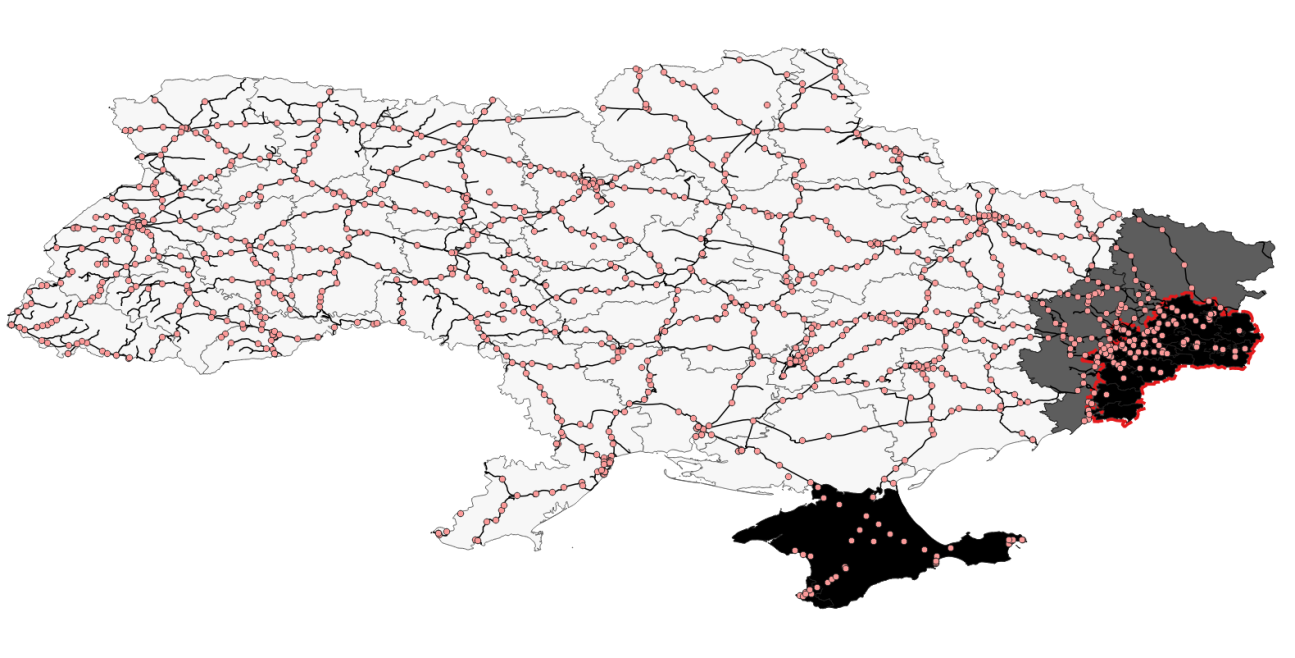
Figure 1: Conflict Areas (2014–2022) and Railroads in Ukraine

Notes: The map highlights the areas directly affected by the 2014 Russia-Ukraine conflict and displays the geographic location of the railroads and the railway stations. The Crimean Peninsula, in black at the bottom of the map, was occupied by Russia in early 2014. The Donetsk People’s Republic (DPR) and Luhansk People’s Republic (LPR) territories are in black with a red rim to the right. The rest of the Donbas region, in light gray, consists of the Donetsk and Luhansk provinces. Black lines indicate the Ukrainian railroads. Red dots represent the railway stations in our railway-shipments data.

2.2   Economic Activity in Donbas and Crimea

Before the conflict, Donbas and Crimea were critically important for Ukraine’s economy. Together, they accounted for about 17.5% of Ukraine’s 2013 GDP. The Donbas region has always been prominent for its extractive industries, especially coal, metallurgy, and manufacturing. Being the most populous province in Ukraine, with 4.4 million people, or 10% of Ukraine’s population, Donetsk oblast (province) has been responsible for more than 20% of all Ukrainian manufacturing and 20% of all Ukraine’s exports as of 2013.

Though less economically important than Donetsk, Luhansk oblast (province) has also been essential for Ukraine; it was the sixth-most-populous Ukrainian province, with 2.16 million people producing 6% of Ukraine’s exports. In contrast to Donbas, Crimea is particularly well-known for its agricultural products and tourism. However, it was also a vital part of Ukraine’s economy before the conflict, hosting 2.2 million people and being the center of several industries, such as shipbuilding.

The consequences of conflict for these regions were devastating. Crimea became almost entirely cut off from the Ukrainian transportation network, leading to a sudden disruption of supply-chain links. The DPR and LPR were overtaken by violence, bombing, destruction of infrastructure and physical capital, and the loss of labor force. In the course of a year, manufacturing production fell by 60% in Donetsk oblast and by 80% in Luhansk oblast. Due to the complexity of the conflict treatment, we will not separately estimate the impacts of each of its components and instead focus on the aggregate consequences of the conflict shock.

2.3   Ukrainian Railroad System

Railway transportation is critical for Ukraine’s economy. Ukraine has the 13th-most-extended railroad network and is the world’s seventh-largest railway freight transporter. Railroads are the main way of transporting products in Ukraine: according to UkrStat, as of 2018, railroads were responsible for 80% of ton-km of all freight transport. Meanwhile, other modes of transportation are not particularly well maintained. According to the WEF Global Competitiveness Report, the Ukrainian railroad infrastructure is among the best in the world (25th in 2013–2014). In contrast, regular roads and airway transportation are poorly ranked relative to those in other countries (144th and 105th in the world in 2013–2014, respectively).

3   Data

In our analysis, we rely on two main datasets. First, we employ novel data on the universe of railroad shipments within Ukraine from 2013 through 2016. These granular data allow us to study the evolution of a production network before and after the start of a large-scale conflict. The dataset contains more than 41 million transactions between more than 7,000 firms. It includes shipment dates, weights (in kg), freight charges, product codes, and station codes filled out my railway clerks. Importantly, the dataset contains unique IDs of the Ukrainian firms-senders and firms-receivers, which enables us to merge the dataset with other firm-level data.

Since Ukrainian railways operate through a state monopoly, no inter-firm railway shipments pass without entering these records. However, to further account for possible mechanical disruptions in data reporting due to the conflict, we exclude the railway shipments conducted fully within the separatist-controlled territories from all of our analysis.

Throughout the paper, we also discard railway shipments passing Ukraine in transit. In contrast, in order to consider all possible alternative buyers and suppliers, we include the Ukrainian firms’ international railway shipments. This choice does not qualitatively affect our estimates as they remain robust to excluding international trade and focusing only on domestic shipments.

Second, we use accounting data from SPARK-Interfax (2017). SPARK-Interfax is similar to the ORBIS/AMADEUS database but has a strong focus on the former Soviet republics, including Russia, Ukraine, Kazakhstan, Belarus, Kyrgyzstan, Uzbekistan, and Moldova. The dataset contains information on firm sales, profits, total costs, capital, and other variables for more than 370,000 Ukrainian firms from 2010 through 2017. Similar to ORBIS/AMADEUS, SPARK-Interfax is based on official government statistics, provision of which is mandatory for all Ukrainian firms except individual entrepreneurs.

LABEL:TABLE:_Summary_Statistics displays the summary statistics for both datasets. On average, a firm sent a shipment to another firm every 13 months. The average weight of the monthly shipments was 257 tons, equivalent to seven railway wagons of coal. In 10.5% of firm pairs, one of them shipped or received either in Donbas or Crimea, and in 62.5% of firm pairs, one of them had a trading partner located either in Donbas or Crimea. Finally, the median total revenue and profits of the firms matched with the SPARK-Interfax dataset over the 2010–2017 period was 26.9 million and 260 thousand Ukrainian hryvnia (around US$1,000,000 and US$10,000 as of November 2021), respectively.

Figure 1 depicts the Ukranian railway network, as well as the 1,200 railway stations in our dataset. The stations cover the entire territory of Ukraine, indirectly confirming the universal nature of our data. As one can see, the railway network is especially dense in the Donbas region. This pattern is consistent with the Donbas’ heavy reliance on railway transportation, given its focus on coal and mineral extraction, metallurgy, and other heavy industry.

4   War and Propagation Through Trade Linkages

In this section, we establish our first main result: the conflict shock not only affects trade between firms directly exposed to violence but also propagates—through the production-network linkages—to trade between firms outside the conflict areas. This result is key for the literature on the economic consequences of wars and violence: it suggests that the standard techniques for comparing conflict and nonconflict areas (e.g., Abadie and Gardeazabal, 2003) may severely underestimate the total economic impact of these events.

To document this result empirically, we estimate a difference-in-differences specification with interfirm trade intensity as an outcome variable and with measures of direct and indirect connections to the conflict areas on the right-hand side of the equation.

We leverage detailed transaction-level data to precisely identify trade links that were directly affected by the annexation of Crimea and the Donbas War. Specifically, we consider the geographic origin of the trade-link nodes, and we study trade between firm-rayon pairs. We consider a particular trade link “first-degree-treated” (i.e., affected directly) if one of the firms was shipping or receiving products directly from or in a conflict-affected rayon. Similarly, we consider a certain trade direction between two firms as “second-degree-treated” (i.e., affected indirectly) if one of the firms traded with the conflict-affected rayons before the start of the conflict, and did so from the same location that they used to ship products within the given trade link. One can think of this approach as performing an establishment-level analysis.

With these caveats in mind, we estimate the following specification:

$$Y_{ijt}=\alpha_{ij}+\kappa_{t}+\beta^{(1)}\times\textnormal{Conflict}_{ij}\times\textnormal{Post}_{t}+\beta^{(2)}\times\textnormal{PartnerConflict}_{ij}\times\textnormal{Post}_{t}+\eta_{ijt}\vspace*{-0.25cm}$$ (1)

where $Y_{ijt}$ represents trade intensity from establishment (firm-rayon) $i$ to establishment $j$ in a given year-month $t$, measured either as probability of trade, log of the number of shipments, or log of the total weight of transactions within a trade link; $\textnormal{Post}_{t}$ is the post-Crimea indicator; $\textnormal{Conflict}_{ij}$ is an indicator for whether the trade link is directly affected by conflict, equal to one if either establishment $i$ or $j$ is in DPR, LPR or Crimea (and zero otherwise); $\textnormal{PartnerConflict}_{ij}$ is an indicator for whether the trade link is affected by conflict one-degree-removed and is equal to one if either $i$ or $j$ had a preconflict partner (other than $j$ or $i$) that was located in DPR, LPR or Crimea and equal to zero otherwise or if either establishment was itself located in DPR, LPR or Crimea; $\alpha_{ij}$ and $\kappa_{t}$ are the establishment-pair(-direction) and year-month fixed effects, respectively. Under an assumption that trade intensity in links with and without first- and second-degree ties to conflict areas evolves along parallel trends, the coefficients $\beta^{(1)}$ and $\beta^{(2)}$ identify the first- and second-degree effects of conflict on trade.

We report the estimated coefficients in Table 4, starting with the first-degree effects only and then adding the second-degree effects. Across all specifications, the first- and second-degree coefficients are negative, statistically significant at the 0.1% level, and of substantial magnitude.

In our preferred specifications, in column (4)–(6), the comparison group consists of the trade links in which no trading partner was in the conflict area and also none of the trading partners had traded with the conflict areas before the start of the conflict. Adding an indirect connection with the conflict—that is, a link through a buyer or a supplier—dampens the monthly probability of trade between two establishments by 2.5 percentage points, a sizeable decline, equivalent to 0.09 standard deviations. If, instead, a trade link was directly connected with the conflict, the monthly probability of trade falls by 13.1 percentage points or 0.49 standard deviations. The results for the log number of shipments and log-weight are qualitatively similar, suggesting that trade volume declines in similar proportions to trade frequency.

Table 1: Propagation of the Conflict Shock Through Interfirm Trade Linkages

	(1)	(2)	(3)	(4)	(5)	(6)
	Any	Log	Log Total	Any	Log	Log Total
	Shipment	Number of	Weight	Shipment	Number of	Weight
		Shipments	Shipped		Shipments	Shipped
Post Crimea $\times$	-0.114∗∗∗	-0.268∗∗∗	-1.487∗∗∗	-0.131∗∗∗	-0.306∗∗∗	-1.715∗∗∗
Either Partner is in Conflict Area	(0.006)	(0.013)	(0.072)	(0.006)	(0.015)	(0.078)
Post Crimea $\times$				-0.025∗∗∗	-0.054∗∗∗	-0.326∗∗∗
Either Partner Traded with Conflict Areas				(0.003)	(0.008)	(0.038)
Establishment-Pair-Direction FE	✓	✓	✓	✓	✓	✓
Year-Month FE	✓	✓	✓	✓	✓	✓
Y Mean	0.077	0.181	1.005	0.077	0.181	1.005
Y SD	0.267	0.724	3.509	0.267	0.724	3.509
R2	0.198	0.279	0.214	0.198	0.279	0.215
Observations	11,001,648	11,001,648	11,001,648	11,001,648	11,001,648	11,001,648
Province Pairs	751	751	751	751	751	751

Notes: This table presents the estimates of equation (1) studying whether interfirm trade declined after the start of the Russia-Ukraine conflict depending on whether one of the partners in an exchange was located in or had traded with the conflict area before the conflict. The outcomes are: an indicator for any shipment from establishment (firm-rayon) $i$ to establishment $j$ at year-month $t$, the logarithm of the total number of shipments from establishment $i$ to establishment $j$ at year-month $t$, and the total weight of these shipments. To avoid missing values, the logarithms add 1 to the value of the argument. Standard errors in parentheses are clustered at the province-pair level. * p$<$0.05, ** p$<$0.01, *** p$<$0.001.

There are two ways in which naïve specifications in columns (1)–(3) underestimate the total impact of conflict on trade. First, the negative second-degree effect contaminates the comparison group leading to a downward bias. Indeed, once we allow for their presence, the first-degree-effect coefficients grow in magnitude—e.g., from $-$0.114 in column (1) to $-$0.131 in column (4) for the monthly probability of trade. Second, the presence of negative second-degree effects, even if small, significantly alters the aggregate calculations of the impact of conflict. This is because the second-degree links with the conflict areas are much more numerous than the first-degree links. In sum, when we aggregate the coefficients up by the number of first- and second-degree connections to the conflict areas, we find that ignoring the second-degree effects leads to underestimation of the total impact of conflict on trade by 65% to 67%, depending on the measure of trade intensity.

Figure 2 illustrates the effects’ dynamics. Specifically, it presents the estimates of the equation (1) but with $\textnormal{Conflict}_{ij}$ and $\textnormal{PartnerConflict}_{ij}$ interacted with the quarterly indicators instead of the post-Crimea indicator. Panel A displays the dynamics of the first-degree effects, and Panel B displays the second-degree effects. The last quarter of 2013 serves as a baseline. Despite some pretrends, Panel A clearly shows that the annexation of Crimea, and especially the escalation of violence in Donbas, has led to a sharp decline in the first-degree trade with the conflict areas. The second-degree effects displayed in Panel B exhibit no pretrends before the conflict, lending strong support for the parallel-trends assumption in this case. The coefficients’ pattern suggests that conflict also has sharp and deep negative indirect consequences appearing immediately with the annexation of Crimea and slowly increasing in magnitude over time.

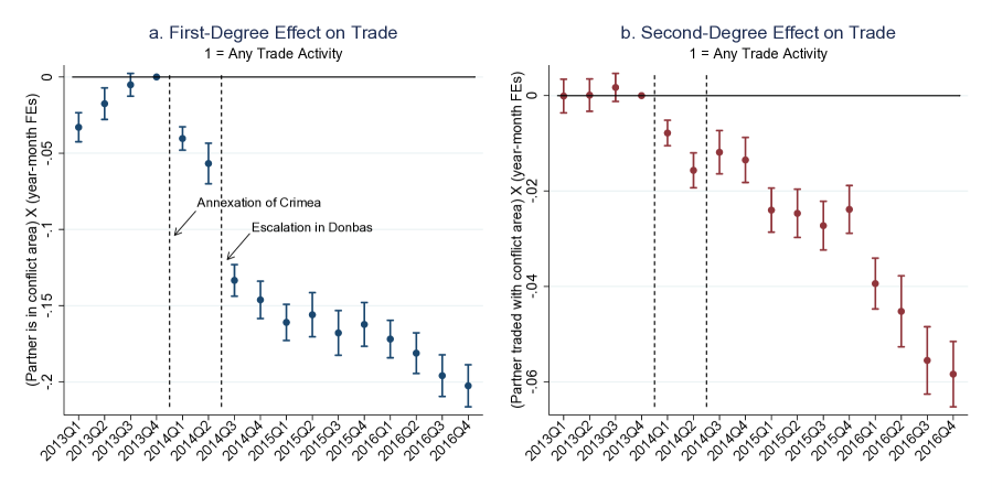
Figure 2: Propagation Effects of Conflict on Trade

Notes: The figure displays the results of estimating a quarter-by-quarter version of equation (1) where first- and second-degree are both interacted with the quarterly indicators. Panel A displays the results for the first-degree (direct) effects of conflict on trade links in which one of the partners was located in the conflict area. Panel B displays the results for the second-degree (indirect) effects of conflict on trade links in which one of the partners had traded with a firm in the conflict areas before the start of the conflict. Bars represent 95% confidence intervals. Standard errors are clustered at the province-pair level. $N=11,001,648$.

Next, we compare upstream and downstream propagation by splitting the data further into having a buyer or a supplier directly or indirectly connected to the conflict areas. Table 7 presents the estimates. In contrast to prior evidence in other contexts (e.g., Carvalho and Tahbaz-Salehi, 2019), the effects indeed differ by the direction of trade. Namely, the first-degree effects are larger if, of the two firms, a buyer was located in the conflict areas (columns 1 through 3). We interpret this disparity as the conflict-induced demand shocks being more severe compared to the supply shocks. For the second-degree effects, the pattern is similar: conflict-induced demand shocks propagate to second-degree links at a higher rate than the conflict-induced supply shocks (columns 4 through 6). One interpretation could be that supply shocks are less severe because of a possible substitution to competing inputs, while the search for new customers in the case of demand shocks is more difficult. Nevertheless, both demand and supply shocks still have sizeable negative second-degree effects, leading to declines in trade frequency in the indirectly connected links of 0.04 and 0.09 standard deviations, respectively.

One may wonder whether the above results are specific to certain industries more prevalent in Donbas or that more heavily rely on the railways as a mode of transportation. To discern the validity of this concern, we present the heterogeneity estimates by firms’ industry. To obtain these estimates, we merge the transaction-level data with each firm’s Standard Industrial Classification (SIC) codes and take the main SIC code listed for each firm. Then, following the official SIC manual (OSHA, 2014), we group the firms into coarse groups of industries, such as mining and manufacturing. Figure A1 presents the heterogeneity estimates. The coefficients are consistent with the intuition that indirect effects should matter most for downstream sectors, such as retail, and matter least for upstream sectors, such as mining. Overall, we note that the degree of heterogeneity is relatively small and, thus, our baseline results are more likely to extend to settings with a different composition of industries and industries with varying reliance on railroad transportation.

Finally, one may be concerned that the results are due to some omitted variable shifted by the conflict and not the production-network propagation. For instance, one may worry that firms with the second-degree connections to the conflict areas could locate geographically closer to the violent areas and, thus, may be more likely to be hit by the concurrent conflict-related demand or supply shocks. Alternatively, second-degree connected firms may locate in provinces of Ukraine that experience relatively more negative indirect effects due to the conflict—e.g., they could host fewer refugees, who present positive labor supply and demand shocks to the local economy. Furthermore, ethnic and historical differences between Donbas, Crimea, and other Ukrainian provinces could have played a role in the post-conflict breakdown of trade (Markevich et al., 2021; Korovkin and Makarin, 2022). We address these concerns with two additional robustness checks. First, we flexibly control for the firm’s distance to the conflict areas interacted with the post-Crimea indicator (Table 7). Second, we control for the province fixed effects interacted with the post-Crimea indicator (Table 7). The results remain qualitatively unchanged.

To summarize, using unique data on within-country trade transactions, we show that the start of a large-scale conflict had a negative impact not only on trade directly associated with the conflict areas but also on trade links connected with them only indirectly. The shock propagates both upstream and downstream, although the demand shock produce larger negative effects. Ignoring the propagation effects leads to severe underestimation of the total economic impact of conflict.

5   War and Firm-Level Effects of Production-Network Structure Change

In this section, we aim to show that a large-scale conflict does not only propagate through the production network but also, if the territorial breakaway is large and persistent—which was the case during the 2014 Russia-Ukraine conflict,—it can change the structure of the production network itself. In turn, this sudden change may have implications for firms in non-conflict areas due to an abrupt shift in their network position.

We illustrate this point empirically by estimating the impact of an exogenous conflict-induced change in firm centrality on several measures of yearly firm performance. A naïve approach would regress the change in firm outcomes on the change in firm centrality between 2013 (before the conflict) and 2014 (after the start of the conflict). However, this regression may suffer from reverse causality—firms with a steeper rise in performance may automatically become more central since they would likely exhibit an increase in the number of transactions and trade with more firms. To preempt this and other similar concerns, we rely on an exogeneous component of the conflict-induced change in firm centrality based on the 2013 production network only. Specifically, we take the 2013 production network, drop the firms in the conflict areas from the network, and recalculate measures of centrality for the remaining firms. Figure A2 illustrates that such predicted firm centrality is highly correlated with the actual firm centrality in 2014. We then take the difference between the predicted measure and the actual firm centrality in 2013. We then estimate the following difference-in-differences equation on levels of firm performance using the exogeneous war-induced change in centrality as the main independent variable:

$$Y_{it}=\alpha_{i}+\delta_{t}+\beta_{t}\times\Delta\widehat{\textnormal{Centrality}}_{i,2013}+\varepsilon_{it}\vspace*{-0.25cm}$$ (3)

where $Y_{it}$ is log-sales or IHS-profits of firm $i$ at year $t$; $\alpha_{i}$ and $\delta_{t}$ are firm and year fixed effects; and $\Delta\widehat{\textnormal{Centrality}}_{i,2013}$ is the exogeneous war-induced change in centrality after the start of the conflict. Under the parallel-trends assumption, $\beta_{t}$’s identify the impact of an exogeneous change in a firm’s network position postconflict on the firm’s subsequent performance.

We use three measures of centrality: eigenvector centrality, betweenness centrality, and degree centrality, and report the results for each of the measures in Figure 3. For all centrality measures, the effects take off in 2014, are persistent, and are generally increasing over time. Before the conflict, firms with different values of predicted centrality evolved along the same trends, which gives credibility to the difference-in-differences design. According to Table 7, which presents the estimates of a version of equation (3) replacing $\beta_{t}$ with a simple pre-post $\beta$, a one-standard-deviation larger exogeneous change in centrality leads to an 8.9% to 14.5% increase in firm’s sales.

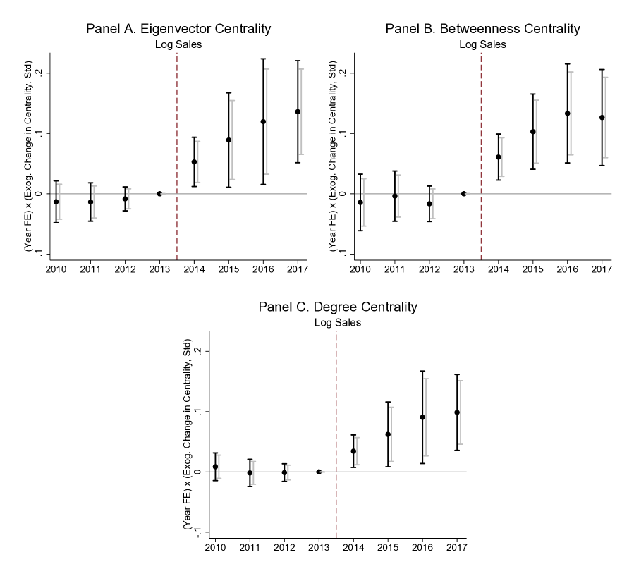
Figure 3: Conflict-Induced Change in Network Centrality and Sales

Notes: This figure displays the results of estimating equation (3). Panel A displays the results for the predicted change in eigenvector centrality between 2013 and 2014 as the interaction variable, Panel B displays the results for the predicted change in log betweenness centrality between 2013 and 2014, and Panel C displays the results for the predicted change in degree centrality between 2013 and 2014. Black bars represent 95% confidence intervals, gray bars represent 90% confidence intervals. All measures of centrality changes are standardized to have zero mean and a standard deviation of one. The sample excludes firms located in the conflict areas. Standard errors are clustered at the firm level. $N=27,201$.

Next, Figure 4 presents the effects on profits and the profits-over-costs ratio. The results are in line with a story in which, in the short-run, firms that become more central charge higher prices which, in turn, translate into higher profits. Both effects dissipate by the end of the study period.

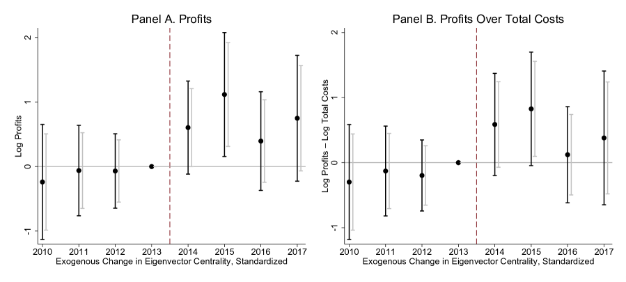
Figure 4: Conflict-Induced Change in Network Centrality, Profits, and Profit-to-Cost Ratio

Notes: This figure displays the results of estimating equation (3). Both panels display the results for the predicted change in eigenvector centrality between 2013 and 2014 as the interaction variable, standardized to have zero mean and standard deviation of one. Panel A presents the results for the inverse hyperbole sine of gross profits as the dependent variable. Panel B presents the results for the inverse hyperbole sine of profits minus the inverse hyperbole sine of total costs as the dependent variable. Black bars represent 95% confidence intervals, gray bars represent 90% confidence intervals. Standard errors are clustered at the firm level.

One may wonder if the results displayed in Figure 3 are simply a mirror image of the propagation effects on trade presented earlier in Section 4. That is, it could be that firms that traded with the conflict areas by definition became less central with the start of the conflict. To assuage this concern, we present two additional exercises. First, we directly control for a firm’s ties with the conflict areas at baseline interacted with the yearly indicators. Figure A3 plots the estimates. Panel A presents the centrality coefficients $\hat{\beta}_{t}$, which appear to be virtually unchanged compared to Figure 3. Panel B reports the marginal negative impact of having conflict ties, one of the mechanisms for which could be the propagation effects on trade documented in Section 4.

Second, we further account for propagation with a residualization exercise. Specifically, we residualize the exogeneous change in centrality from firms’ baseline characteristics, such as whether a firm traded with someone in the conflict areas, the share of its transactions being with the conflict areas, the share of its total sales being with the conflict areas, the total weight of its partners’ trade with the conflict areas (i.e., through second-degree connections), as well as the firm’s baseline sales and profits. We then use the obtained residuals as a measure of exogenous change in centrality in equation (3). The results presented in Figure A4 further confirm that the results in Figure 3 remain robust to controlling for indirect exposure to conflict.

Overall, these results detail a previously undocumented indirect effect of conflict, and possibly other large persistent shocks cutting off certain regions from trade with the rest of the country, on firms through a change in the production-network structure. We confirm such effect’s existence by showing that Ukrainian firms which, for reasons beyond their control, became more central with the start of the Russia-Ukraine conflict gained (or lost less) in terms of sales and profits. We speculate that these effects may be due to a temporary surge in those firms’ relative market power.

6   War, Network Destruction, and Network Adjustment

So far, we have documented that a large-scale secessionist conflict (i) disrupts trade, and this disruption propagates even to trade links in nonconflict areas, and (ii) alters the structure of the production network, which on its own affects firm performance. In this section, we go a step beyond relative comparisons and use a theoretical model to explore the war-induced absolute changes to revenue distribution in several counterfactual scenarios. Most crucially, we quantify the importance of endogenous network formation for economic recovery from a large negative shock.

6.1   Model

We build a general equilibrium model of production networks in the spirit of Long Jr and Plosser (1983), Acemoglu et al. (2012), and Baqaee and Farhi (2019). The model allows us to explore three counterfactuals: (i) the first one corresponds to network destruction before firms manage to adjust to the new equilibrium and redirect their input and output flows; (ii) the second one corresponds to the observed network adjustment of the firms; (iii) the third counterfactual focuses only on the outside demand changes after the conflict, keeping the production network fixed at the preconflict level.

To accomodate these counterfactuals, we depart from the standard Cobb-Douglas production function (e.g., Acemoglu et al., 2012) in favor of a more general constant elasticity of substitution (CES) technology. Specifically, in our hypothetical economy, a generic firm $i$ uses a bundle of intermediate inputs described by a CES aggregator: $M_{i}=\Big{(}\sum_{j=1}^{n}a_{ji}^{1/\sigma}x_{ji}^{(\sigma-1)/\sigma}\Big{)}^{\frac{\sigma}{\sigma-1}}$ where $x_{ji}$ is the amount of good $j$ used in production of good $i$ and $a_{ji}$ is the share of input $j$ needed for good $i$. We assume constant returns to scale for intermediate inputs; that is, $\sum_{j=1}^{n}a_{ji}=1$.

The substitution patterns between the CES intermediate-input aggregator, $M_{i}$, and the only other factor, labor $l_{i}$, take a Cobb-Douglas form with constant returns to scale. In this case, output $x_{i}$ of firm $i$ can be written as:

$$x_{i}=(z_{i}l_{i})^{\alpha}\Big{(}\sum_{j=1}^{n}a_{ji}^{1/\sigma}x_{ji}^{(\sigma-1)/\sigma}\Big{)}^{\frac{\sigma}{\sigma-1}(1-\alpha)}\vspace*{-0.25cm}$$

where $z_{i}$ is firm-specific productivity, $l_{i}$ is the amount of labor hired, and $x_{ji}$ is the input of good $j$ used in the production of output $i$.

We assume no free entry, which corresponds to a short- or medium-run case, and firms earn positive profits in equilibrium with constant markups.

We combine the CES production technology with CES preferences over $n$ goods, so the consumer maximizes the following utility function:

$$u(c_{1},...,c_{n})=\Big{(}\sum_{i=1}^{n}c_{i}^{\eta}\Big{)}^{1/\eta}\vspace*{-0.25cm}$$

The constant across-goods elasticity of substitution is $1/(1-\eta)$ in this case.

The supply of labor is inelastic, with the total labor in the economy normalized to $L$. Wages are denoted by $w$.

A competitive equilibrium of our railway economy with $n$ firms and $n$ differentiated goods consists of the price vector $\mathbf{p}$, wage $w$, consumption vector c, and quantities $(l_{i},x_{i},\mathbf{x_{ji}})$ such that (i) the representative consumer maximizes utility; (ii) representative firms maximize their profits given the prices; (iii) all markets clear:

$$x_{i}=\sum_{j=1}^{n}x_{ij}+c_{i},\ \forall\ i,\sum_{i=1}^{n}l_{i}=L\vspace*{-0.25cm}$$

Expressing $x_{ij}$ from the first-order condition of the firms’ profit-maximization problem (see the derivations in Appendix C), we obtain:

$$r_{i}=(1-\alpha)\sum_{j=1}^{n}\underbrace{\frac{a_{ij}/p_{i}^{1-\sigma}(\mathbf{a})}{\sum_{m}a_{mj}/p_{m}^{1-\sigma}(\mathbf{a})}}_{\text{I-O weight }\omega_{ij}(\mathbf{a})}\cdot r_{j}+\underbrace{p_{i}c_{i}}_{\text{outside demand }\bm{\xi}}\vspace*{-0.25cm}$$

We can summarize the input-output linkages with matrix $\mathbf{\Omega}$, which simultaneously represents two things: the adjacency matrix observed in the data, and the economy’s steady-state input-output matrix. Concise matrix notation allows us to rewrite the central equation as one relating the vector of revenues, outside demand, and the input-output matrix in the economy:

$$\mathbf{r}=(1-\alpha)\mathbf{\Omega}\mathbf{r}+\bm{\xi}\vspace*{-0.25cm}$$ (5)

Note that $\mathbf{\Omega}$ and $\mathbf{r}$ are observed in the data, and each element of the matrix is defined by the equilibrium weights, $\omega_{ij}(\mathbf{a})=\frac{a_{ij}/p_{i}^{1-\sigma}(\mathbf{a})}{\sum_{m}a_{mj}/p_{m}^{1-\sigma}(\mathbf{a})}$. Vector $\bm{\xi}$ is the outside demand vector, which includes both consumer demand and demand from firms outside the railway network.

If $\sigma\rightarrow 1$, our production function converges to Cobb-Douglas and elements of $\mathbf{\Omega}$ ($\omega_{ij}$) converge to constants proportional to $a_{ij}$. The main difference between our CES aggregator and the Cobb-Douglas is that zero inputs for some intermediate goods does not automatically mean zero production for the firms. However, with the CES production function, solving for the equilibrium in a closed form becomes impossible. Our empirical exercise overcomes the intractability of the model by manipulating $\mathbf{\Omega}$ directly.

6.2   Counterfactuals

For the empirical part of this exercise, we add yearly indices $t$ to the input-output matrix equation (5) to get:

$$[\mathbf{I}-(1-\alpha^{t})\mathbf{\Omega}^{t}]\mathbf{r}^{t}=\bm{\xi}^{t}$$ (6)

where $\mathbb{I}$ is an identity matrix. Following the notation in Section 6.1, $\mathbb{\Omega}^{t}$ is the railway firm-level input-output matrix; $\mathbb{r}^{t}$ is a vector of firms’ total revenues in year $t$; $\alpha^{t}$ is the labor share in production (or any non-intermediate-factor share in our case) in year $t$; and $\bm{\xi}^{t}$ is yearly outside demand. We fix labor share to be constant in time $\alpha^{t}=\alpha$ and allow revenues, final demand, and the input-output matrix to vary flexibly over $t$. We then plug in $\mathbb{r}^{t}$ and $\mathbb{\Omega}^{t}$ in order to back out the final demand $\bm{\xi}^{t}$. One key advantage of our data is that we observe the realized $\mathbb{\Omega}^{t}$ and thus can vary it to explore different counterfactuals relating production-network structure and firm revenue.

The first counterfactual we explore gets at the aggregate impact of the initial shock of war to the production-network structure. It corresponds to the change from $\mathbb{\Omega^{2013}}$ to $\mathbb{\tilde{\Omega}^{2013}}$, which is the 2013 network but with zeros in place of trade with the firms in the conflict areas (object similar to the one used in Section 5). Final demand is kept constant at $\bm{\xi^{2013}}$. This counterfactual quantifies the network-destruction channel.

The second counterfactual has to do with the economy’s adjustment. Specifically, after the initial shock, firms may have found new buyers and suppliers within the nonconflict areas, and this readjustment could have mitigated the initial impact of the war. To reflect this change, we keep the final demand at the 2013 level, $\bm{\xi^{2013}}$, and we plug in the new network structure from 2014, $\mathbb{\Omega^{2014}}$. The difference between the resulting change and the change in the network-destruction counterfactual quantifies the network-adjustment channel.

Finally, to be transparent about all of the forces that drive the change before and after conflict, we also consider the outside-demand counterfactual. Specifically, we assess the size of the outside demand shock by keeping the railway production network at $\mathbb{\Omega}^{2013}$ and varying the final demand from $\bm{\xi^{2013}}$ to $\bm{\xi^{2014}}$. To estimate $\bm{\xi^{2013}}$ and $\bm{\xi^{2014}}$, we plug in $(\mathbb{\Omega^{t}},\mathbb{r}^{t}),\ t=\{2013,2014\}$.

Table 2 presents the results for each counterfactual. Column 2 of Table 2 reports the change in the median of the distribution, corresponding to the network-destruction channel. Network destruction leads to a substantial $46.8\%$ drop in the median firm revenue in nonconflict areas.

Column 3 of Table 2 suggests that, if the production network were allowed to readjust and firms were allowed to find new partners, the initial shock to the network structure manifested by the changes in $\mathbb{\Omega}^{t}$ would be mitigated substantially. Network adjustment compensates for around 80% of the network destruction for the firm median revenue in nonconflict areas, with a total decline of $-$9.7% relative to the baseline.

Column 4 of Table 2 displays the results for the outside-demand counterfactual. The demand shock is equivalent to a $17.3\%$ decline in the median of the revenue distribution, i.e., smaller than network destruction in magnitude but larger than if firms are allowed to adjust their network.

Finally, we can compare all of these channels to the total observed change, which is $-27.2\%$ relative to the 2013 baseline (column 5). The actual change in this case turns out to be a rough sum of the network-adjustment and outside-demand effects.

To summarize the above, the exogenous change in production-network structure due to conflict not only creates relative winners and losers, as in Section 5, but also moves the distribution of firm revenue down, decreasing the median firm revenue in the rest of the country by 46.8%. However, readjustment after the start of the conflict within the remaining network compensates four-fifths of the latter decline, suggesting that endogenous network formation compensates for most of the initial shock. The following section explores the dynamics of these two effects, considers changes along the whole distribution, and extends the counterfactuals to all firms in the economy in an aggregation exercise.

Table 2: Counterfactuals

	(1)	(2)	(3)	(4)	(5)
	$\mathbb{r}(\mathbb{\Omega^{2013}},\bm{\xi^{2013}})$	$\mathbb{r}(\mathbb{\tilde{\Omega}^{2013}},\bm{\xi^{2013}})$	$\mathbb{r}(\mathbb{\Omega^{2014}},\bm{\xi^{2013}})$	$\mathbb{r}(\mathbb{\Omega^{2013}},\bm{\xi^{2014}})$	$\mathbb{r}(\mathbb{\Omega^{2014}},\bm{\xi^{2014}})$
	Baseline	Network Destruction	Network Adjustment	Outside Demand	Total Change
$\text{Median}(\mathbb{r})$, Mln. 2010 US$	2.26	1.20	2.03	1.86	1.64
Relative to 2013	0%	-46.8%	-9.7%	-17.3%	-27.2%
$N$	4,463	4,463	4,463	4,463	4,463

Notes: The table presents the counterfactual estimates. Specifically, we obtain the vector of revenues $\bm{r}$ for a given input-output matrix $\mathbb{\Omega}$ and outside demand $\bm{\xi}$ such that $\bm{r}(\bm{\xi},\mathbb{\Omega}):=[\mathbb{I}-(1-\alpha)\mathbb{\Omega}]^{-1}\bm{\xi}$, and we present the median revenue of the resulting distributions. Columns vary each of the arguments. Column (1) displays the actual median firm revenue in 2013. Column (2) uses the modified 2013 input-output matrix, where links with firms from the conflict areas are replaced with zeros, $\mathbb{\tilde{\Omega}^{2013}}$. Column (3) fixes the outside demand at the 2013 level and uses the actual 2014 input-output matrix, $\mathbb{\Omega^{2014}}$. Column (4) uses the 2014 outside demand and the 2013 input-output matrix, $\mathbb{\Omega^{2013}}$. Column (5) displays the actual median firm revenue in 2014. The sample is restricted to firms in nonconflict areas. All quantities are expressed in 2010 US$.

6.3   Additional Results: Interfirm Inequality and Dynamics of Network Adjustment

Interfirm inequality.

While the change in the median is a crucial summary statistic for our counterfactuals, one might also ask what happens to other parts of the firm revenue distribution. As it turns out, the initial conflict shock and the subsequent network adjustment led to an increase in inequality between firms. To document it, we extend the estimates in Table 2 to other features of the firm-revenue distribution and compare the network-adjustment counterfactual to the network-destruction scenario and the observed data for firms at the left and right tails.

Table A8 presents the results. Column 3 of Table A8 suggests that firms at the 75th percentile of the distributions gain 14.0% of their 2013 revenues in the network-adjustment counterfactual—compared to both the observed loss of 22.8% in column 5 and the loss of 29.3% in the network-destruction counterfactual in column 2. Hence, we find that, at the right tail of the distribution, network adjustment fully compensates for the loss of revenue due to network destruction and even leads to some gains. In contrast, at the 25th percentile of the distribution, firms lose slightly more under the network-adjustment scenario than in the observed data—a 62.3% vs. 62.0% drop. Moreover, network adjustment compensates for only 32.5% of the network destruction at the left tail—much less than at the median. Overall, the estimates imply that, controlling for outside shocks and other factors, large adverse shocks to portions of the network and subsequent network adjustment exacerbate interfirm inequality and may lead to greater concentration.

Dynamics. Another natural question to ask is whether network adjusted immediately or whether this process stretched over time, e.g., due to switching costs, and thus compensated for more and more of the initial network-destruction shock as time went on.

To study the medium-run effects of the network adjustment to conflict, Figure 5 plots the medians and the interquartile ranges of 2013–2016 firm revenue. We find that, under the network-adjustment counterfactual, median revenue did not vary across years: it initially changed by $-$9.7% in 2014, then stayed low at $-$9.9% in 2015 and $-$9.4% in 2016 (all relative to the 2013 median).

Instead, we find substantial dynamics at the tails of the distribution. Specifically, the 75th percentile under network adjustment grew by 14.0% in 2014, 21.4% in 2015, and by 28.0% in 2016 relative to the same point in the revenue distribution in 2013. At the same time, the 25th percentile declined by $-$62.3% in 2014, $-$73.0% in 2015, and by $-$77.5% in 2016. The 40th-to-60th-percentile ranges in Figure 5 further confirm this pattern.

Thus, the endogeneous network-adjustment channel, controlling for outside demand and other factors, pushes toward increased interfirm inequality and concentration over time, with little growth at the median after the initial adjustment.

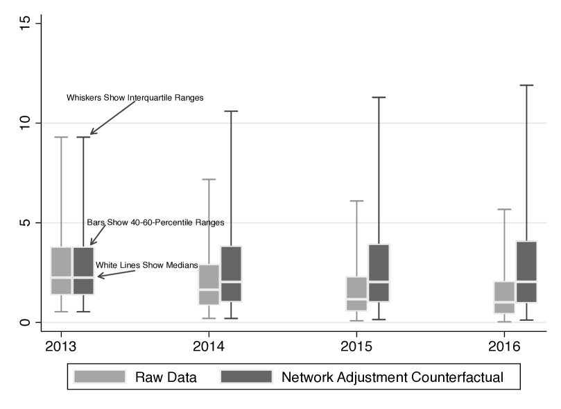
Figure 5: Network-Adjustment Counterfactual and Actual Changes Over Time

Notes: The graph depicts the 2013–2016 evolution of two firm revenue distributions: the one we actually observe in the data (in light grey) and the one we derive under the network-adjustment counterfactual scenario (in dark grey). The “whiskers” represent the interquartile range, and the bars represent the 40th-to-60th-percentile range of each distribution. The network-adjustment counterfactual scenario is derived by fixing the outside demand at the 2013 level, $\bm{\xi}^{2013}$, and changing the input-output matrix gradually, $\mathbb{\Omega}^{t}:\ t=\{2013,2014,2015,2016\}$. All quantities are expressed in 2010 $US. $N$=4,463 per year. The sample is a balanced panel of the 2013 firms.

6.4   Extrapolating Beyond the Railway Network of Firms

At the final step of analysis, we address the question of external validity of our results in the third part of the paper outside the railway network of firms. To do so, we aggregate our estimates to the near universe of all firms in the economy and compare the overall change and the network-adjustment counterfactual at a higher geographical level.

To do so, we redefine the vector of revenues and the matrix of connections at the province and district levels. We take the total of all firm revenues for a given geographic unit and year as the $\mathbb{r}$ input. We proxy for the aggregate-level $\mathbb{\Omega}$ using railway data by summing up all transactions for each pair of localities. The disadvantage of this exercise is that it assumes that the measurement error of connections is similar across locality pairs. However, it extends the external validity of our results by focusing on the near-universe of firms in the economy rather than only on firms relying on the rail transport.

We assess the results of this aggregate counterfactual estimation in two steps. First, we plot the province- and district-level maps in Figures A7 and A8, respectively, with the top maps in both figures representing the observed changes and the bottom maps representing the network-adjustment counterfactual changes. At both aggregation levels, network adjustment smoothens the changes compared to the observed data. What is especially evident from the figures, particularly for the more granular depiction at the district level, is that areas near but just outside the conflict zones take a big hit in the observed data but can benefit under the network-adjustment scenario. This finding highlights the mechanics of our network-adjustment exercise: it controls for outside demand shocks but allows for reallocation of trade within the rest of the country, with nearby districts seemingly serving as a good substitute for production in the conflict areas.

Second, in Table A10, we collapse these geographic patterns into one number—countrywide total revenue. Total revenues coming from the province-level estimates in columns (2) and (3) and the district-level estimates in columns (4) and (5) are largely similar. They exhibit a deterioration in the raw data but a gradual increase in the adjustment counterfactual. Overall, these results are in line with the intuition that network adjustment represents a tool for economic recovery.

7   Conclusion

Over the past few decades, the world has become exceedingly interconnected, and production networks have grown ever more complex. On one hand, due to increased complexity, economic systems have become vulnerable to large shocks. On the other hand, any such shocks are now easier to absorb due to an increased number of potential substitutes. Given these worldwide trends, it is now increasingly important to study how modern production networks react to big shocks, such as wars or pandemics, how quickly they are able to readjust, and which firms stand to gain or lose as a result. Despite recent progress in this research agenda, evidence remains limited, both in terms of research questions and its regional scope.

In this paper, we examine the consequences of a particular massive shock to the economy—large-scale conflict. Specifically, we study the ramifications of the 2014 Donbas war and the annexation of Crimea for the Ukrainian economy. Using novel data on the universe of Ukrainian firm-to-firm railway shipments in 2013–2016, we document that the conflict shock did indeed propagate throughout the production network and spill over onto the rest of the country. Trade has significantly decreased, even between firms outside of the conflict areas, if one of them had a trade partner in Donbas or Crimea before the start of the conflict.

We then study the consequences of the shock to the production-network structure by which firms in three large regions became virtually cut off from the rest of the economy. We find that firms which, for exogenous reasons, became more central have experienced significant permanent gains in sales. These are accompanied by temporary gains in profits and the profits-over-total-costs ratio, suggesting increased market power as a plausible mechanism. Finally, estimating counterfactuals in a production-network model, we show that production-network adjustment would be able to mitigate 80% of the losses in median firm revenue after the initial network-destruction shock, keeping outside factors the same.

Overall, our results suggest that large shocks not only propagate through the network but also may alter its structure, with potentially significant implications for the economy in the medium run. Our results should be of interest to academics and policymakers interested in estimating, predicting, and mitigating the economic consequences of conflicts and other large economic shocks.

Despite the numerous differences between the 2014 Russia-Ukraine conflict and the full-scale Russian invasion of Ukraine in February 2022, our estimates offer a unique glimpse into the potential economic consequences of the ongoing conflict that have not yet been discussed in the academic literature. We hope that future research will shed more light on the full ramifications of the latter episode.

Appendix A: Additional Tables and Figures

Notes: This table provides a version of the baseline results from equation (1) and Table 4 focusing on the firm-level instead of the establishment-level second-degree conflict treatment. The outcomes are: an indicator for any shipment from establishment (firm-rayon) $i$ to establishment $j$ at year-month $t$, the logarithm of the total number of shipments from establishment $i$ to establishment $j$ at year-month $t$, and the total weight of these shipments. To avoid missing values, the logarithms contain 1 inside. Standard errors in parentheses are clustered at the province-pair level. * p$<$0.05, ** p$<$0.01, *** p$<$0.001.

Table A3: Propagation of the Conflict Shock: Borusyak and Hull (2020) Adjustment

	(1)	(2)	(3)	(4)	(5)	(6)
	Any	Log	Log Total	Any	Log	Log Total
	Shipment	Number of	Weight	Shipment	Number of	Weight
		Shipments	Shipped		Shipments	Shipped
Post Crimea $\times$	-0.115∗∗∗	-0.271∗∗∗	-1.505∗∗∗	-0.127∗∗∗	-0.298∗∗∗	-1.663∗∗∗
Either Partner is in Conflict Area	(0.005)	(0.013)	(0.070)	(0.006)	(0.014)	(0.078)
Post Crimea $\times$				-0.018∗∗∗	-0.040∗∗∗	-0.230∗∗∗
Either Partner Traded with Conflict Areas				(0.002)	(0.005)	(0.025)
Post Crimea $\times$	-0.000∗∗∗	-0.001∗∗∗	-0.005∗∗∗	-0.000∗∗∗	-0.001∗∗∗	-0.004∗∗∗
Number of Buyer’s Partners in 2013	(0.000)	(0.000)	(0.000)	(0.000)	(0.000)	(0.000)
Post Crimea $\times$	-0.000∗∗∗	-0.000∗	-0.001∗∗∗	-0.000	-0.000	-0.000
Number of Supplier’s Partners in 2013	(0.000)	(0.000)	(0.000)	(0.000)	(0.000)	(0.000)
Establishment-Pair-Direction FE	✓	✓	✓	✓	✓	✓
Year-Month FE	✓	✓	✓	✓	✓	✓
Y Mean	0.077	0.181	1.005	0.077	0.181	1.005
Y SD	0.267	0.724	3.509	0.267	0.724	3.509
R2	0.198	0.279	0.215	0.199	0.279	0.215
Observations	11,001,648	11,001,648	11,001,648	11,001,648	11,001,648	11,001,648
Province Pairs	751	751	751	751	751	751

Notes: This table provides a version of the baseline results from equation (1) and Table 4 using an adjustment in the spirit of Borusyak and Hull (2020) controlling for the number of supplier’s and buyer’s preconflict partners interacted with the postconflict indicator. The outcomes are: an indicator for any shipment from establishment (firm-rayon) $i$ to establishment $j$ at year-month $t$, the logarithm of the total number of shipments from establishment $i$ to establishment $j$ at year-month $t$, and the total weight of these shipments. To avoid missing values, the logarithms contain 1 inside. Standard errors in parentheses are clustered at the province-pair level. * p$<$0.05, ** p$<$0.01, *** p$<$0.001.

Table A4: Propagation of the Conflict Shock: Downstream and Upstream Effects

	(1)	(2)	(3)	(4)	(5)	(6)
	Any	Log	Log Total	Any	Log	Log Total
	Shipment	Number of	Weight	Shipment	Number of	Weight
		Shipments	Shipped		Shipments	Shipped
Post Crimea $\times$	-0.098∗∗∗	-0.241∗∗∗	-1.289∗∗∗	-0.097∗∗∗	-0.243∗∗∗	-1.283∗∗∗
Supplier is in Conflict Area	(0.007)	(0.017)	(0.093)	(0.008)	(0.017)	(0.097)
Post Crimea $\times$	-0.138∗∗∗	-0.310∗∗∗	-1.791∗∗∗	-0.147∗∗∗	-0.325∗∗∗	-1.900∗∗∗
Buyer is in Conflict Area	(0.007)	(0.018)	(0.088)	(0.007)	(0.019)	(0.090)
Post Crimea $\times$				-0.011∗∗∗	-0.027∗∗∗	-0.148∗∗∗
Either Partner Had Supplier in Conflict Area				(0.002)	(0.005)	(0.027)
Post Crimea $\times$				-0.023∗∗∗	-0.043∗∗∗	-0.294∗∗∗
Either Partner Had Buyer in Conflict Area				(0.003)	(0.008)	(0.039)
Establishment-Pair-Direction FE	✓	✓	✓	✓	✓	✓
Year-Month FE	✓	✓	✓	✓	✓	✓
Y Mean	0.077	0.181	1.005	0.077	0.181	1.005
Y SD	0.267	0.724	3.509	0.267	0.724	3.509
R2	0.198	0.279	0.214	0.198	0.279	0.215
Observations	11,001,648	11,001,648	11,001,648	11,001,648	11,001,648	11,001,648
Province Pairs	751	751	751	751	751	751

Notes: This table presents the estimates of equation (2) studying whether interfirm trade declined after the start of the Russia-Ukraine conflict depending on whether one of the partners in an exchange located in or have at any point traded with the conflict area. In contrast to equation (1), this specification separates between upstream and downstream shock propagation. The outcomes are: an indicator for any shipment from establishment (firm-rayon) $i$ to establishment $j$ at year-month $t$, the logarithm of the total number of shipments from establishment $i$ to establishment $j$ at year-month $t$, and the total weight of these shipments. To avoid missing values, the logarithms contain 1 inside. All specifications exclude trade links in which both partners are located in the conflict areas. Standard errors in parentheses are clustered at the province-pair level. * p$<$0.05, ** p$<$0.01, *** p$<$0.001.

Table A5: Propagation of the Conflict Shock: Controlling For Firms’ Distance to Conflict Areas

	(1)	(2)	(3)	(4)	(5)	(6)
	Any	Log	Log Total	Any	Log	Log Total
	Shipment	Number of	Weight	Shipment	Number of	Weight
		Shipments	Shipped		Shipments	Shipped
Post Crimea $\times$	-0.109∗∗∗	-0.258∗∗∗	-1.424∗∗∗	-0.131∗∗∗	-0.307∗∗∗	-1.715∗∗∗
Either Partner is in Conflict Area	(0.005)	(0.012)	(0.067)	(0.005)	(0.013)	(0.067)
Post Crimea $\times$				-0.030∗∗∗	-0.065∗∗∗	-0.386∗∗∗
Either Partner Traded with Conflict Areas				(0.002)	(0.005)	(0.024)
Post Crimea $\times$	✓	✓	✓	✓	✓	✓
5th Polynomial of Sender’s Distance to Conflict Areas
Post Crimea $\times$	✓	✓	✓	✓	✓	✓
5th Polynomial of Receiver’s Distance to Conflict Areas
Establishment-Pair-Direction FE	✓	✓	✓	✓	✓	✓
Year-Month FE	✓	✓	✓	✓	✓	✓
Y Mean	0.076	0.174	0.984	0.076	0.174	0.984
Y SD	0.264	0.707	3.470	0.264	0.707	3.470
R2	0.195	0.278	0.212	0.196	0.278	0.213
Observations	9,035,232	9,035,232	9,035,232	9,035,232	9,035,232	9,035,232
Province Pairs	710	710	710	710	710	710

Notes: This table provides a version of the baseline results from equation (1) and Table 4 but flexibly controlling for the sender’s and receiver’s spherical distance to the conflict areas. The outcomes are: an indicator for any shipment from establishment (firm-rayon) $i$ to establishment $j$ at year-month $t$, the logarithm of the total number of shipments from establishment $i$ to establishment $j$ at year-month $t$, and the total weight of these shipments. To avoid missing values, the logarithms contain 1 inside. Standard errors in parentheses are clustered at the province-pair level. * p$<$0.05, ** p$<$0.01, *** p$<$0.001.

Table A6: Propagation of the Conflict Shock: Controlling For Post-Province FE

	(1)	(2)	(3)	(4)	(5)	(6)
	Any	Log	Log Total	Any	Log	Log Total
	Shipment	Number of	Weight	Shipment	Number of	Weight
		Shipments	Shipped		Shipments	Shipped
Post Crimea	-0.077∗∗∗	-0.177∗∗∗	-1.000∗∗∗	-0.103∗∗∗	-0.233∗∗∗	-1.332∗∗∗
Either Partner is in Conflict Area	(0.004)	(0.010)	(0.052)	(0.004)	(0.010)	(0.053)
Post Crimea				-0.029∗∗∗	-0.064∗∗∗	-0.379∗∗∗
Either Partner Traded with Conflict Areas				(0.002)	(0.004)	(0.022)
Establishment-Pair-Direction FE	✓	✓	✓	✓	✓	✓
Post Crimea-Province FE	✓	✓	✓	✓	✓	✓
Year-Month FE	✓	✓	✓	✓	✓	✓
Y Mean	0.077	0.181	1.005	0.077	0.181	1.005
Y SD	0.267	0.724	3.509	0.267	0.724	3.509
R2	0.200	0.280	0.216	0.200	0.280	0.217
Observations	11,001,648	11,001,648	11,001,648	11,001,648	11,001,648	11,001,648
Province Pairs	751	751	751	751	751	751

Notes: This table provides a version of the baseline results from equation (1) and Table 4 but controlling for the post-Crimea indicator interacted with the province indicators. The outcomes are: an indicator for any shipment from establishment (firm-rayon) $i$ to establishment $j$ at year-month $t$, the logarithm of the total number of shipments from establishment $i$ to establishment $j$ at year-month $t$, and the total weight of these shipments. To avoid missing values, the logarithms contain 1 inside. Standard errors in parentheses are clustered at the province-pair level. * p$<$0.05, ** p$<$0.01, *** p$<$0.001.

Table A7: Effect of Conflict on Firm Performance Through Change in Network Structure

	Logarithm Sales			IHS Profits
	(1)	(2)	(3)	(4)	(5)	(6)
Post Crimea $\times$ Change in Eigenvector Centrality	0.145∗∗∗			0.679∗∗
	(0.039)			(0.262)
Post Crimea $\times$ Change in Betweenness Centrality		0.118∗∗∗			0.684∗∗∗
		(0.030)			(0.195)
Post Crimea $\times$ Change in Degree Centrality			0.089∗∗			0.382∗
			(0.028)			(0.192)
Firm FE	✓	✓	✓	✓	✓	✓
Year FE	✓	✓	✓	✓	✓	✓
Mean	17.062	17.062	17.062	6.941	6.941	6.941
SD	2.444	2.444	2.444	13.036	13.036	13.036
R2	0.81	0.81	0.81	0.47	0.47	0.47
Observations	30,209	30,209	30,209	29,495	29,495	29,495
Number of Firms	3,997	3,997	3,997	3,970	3,970	3,970

Notes: This table presents the estimates of equation (3) studying whether firms that for exogenous reasons experienced a change in their production-network centrality changed their relative performance after the start of the conflict. All measures of centrality change are standardized to have mean zero and standard deviation of one. The sample is restricted to firms outside of the conflict areas (i.e., DPR, LPR, and Crimea). The dependent variable in Columns (1)–(3) is the logarithm of sales calculated as $L(X)=log(1+X)$. The dependent variable in Columns (4)–(6) is the inverse hyperbolic sine of gross profit calculated as $L(X)=log(X+\sqrt{X^{2}+1})$ following MacKinnon and Magee (1990). Standard errors in parentheses are clustered at the firm level. * p$<$0.05, ** p$<$0.01, *** p$<$0.001.

Table A8: Counterfactuals—Other Features of Distributions, Baseline Sample

	(1)	(2)	(3)	(4)	(5)
	$\mathbb{r}(\mathbb{\Omega^{2013}},\bm{\xi^{2013}})$	$\mathbb{r}(\mathbb{\tilde{\Omega}^{2013}},\bm{\xi^{2013}})$	$\mathbb{r}(\mathbb{\Omega^{2014}},\bm{\xi^{2013}})$	$\mathbb{r}(\mathbb{\Omega^{2013}},\bm{\xi^{2014}})$	$\mathbb{r}(\mathbb{\Omega^{2014}},\bm{\xi^{2014}})$
	Baseline	Network Destruction	Network Adjustment	Outside Demand	Total Change
Median $\mathbb{r}$	2.25	1.20	2.03	1.86	1.64
Relative to 2013	0.0%	-46.8%	-9.7%	-17.3%	-27.2%
25th %-tile $\mathbb{r}$	0.54	0.04	0.20	0.13	0.20
Relative to 2013	0.0%	-92.9%	-62.3%	-76.0%	-62.0%
75th %-tile $\mathbb{r}$	9.29	6.57	10.59	9.58	7.17
Relative to 2013	0.0%	-29.3%	14.0%	3.1%	-22.8%
Mean $\mathbb{r}$	30.27	12.02	26.94	25.78	24.99
Relative to 2013	0.0%	-60.3%	-11.0%	-14.8%	-17.4%
$N$	4,463	4,463	4,463	4,463	4,463

Notes: The table presents the extended version of the counterfactual estimates in Table 2. Specifically, we obtain the vector of revenues $\bm{r}$ for a given input-output matrix $\mathbb{\Omega}$ and outside demand $\bm{\xi}$ such that $\bm{r}(\bm{\xi},\mathbb{\Omega}):=[\mathbb{I}-(1-\alpha)\mathbb{\Omega}]^{-1}\bm{\xi}$ and present four summary statistics of the resulting distributions: median, 25th percentile, 75th percentile, and the mean. Columns vary each of the arguments. Column (1) displays the actual revenue statistic in 2013. Column (2) uses the modified 2013 input-output matrix where trade with firms from the conflict areas is replaced with zeros, $\mathbb{\tilde{\Omega}^{2013}}$. Column (3) fixes the outside demand at the 2013 level and uses the actual 2014 input-output matrix, $\mathbb{\Omega^{2014}}$. Column (4) uses the 2014 outside demand and the 2013 input-output matrix, $\mathbb{\Omega^{2013}}$. Column (5) displays the actual revenue statistic in 2014. The sample is restricted to firms in nonconflict areas. All quantities are expressed in 2010 $US.

Table A9: Counterfactuals—Other Features of Distributions, Sample of All Firms

	(1)	(2)	(3)	(4)	(5)
	$\mathbb{r}(\mathbb{\Omega^{2013}},\bm{\xi^{2013}})$	$\mathbb{r}(\mathbb{\tilde{\Omega}^{2013}},\bm{\xi^{2013}})$	$\mathbb{r}(\mathbb{\Omega^{2014}},\bm{\xi^{2013}})$	$\mathbb{r}(\mathbb{\Omega^{2013}},\bm{\xi^{2014}})$	$\mathbb{r}(\mathbb{\Omega^{2014}},\bm{\xi^{2014}})$
	Baseline	Network Destruction	Network Adjustment	Outside Demand	Total Change
Median $\mathbb{r}$	1.85	0.93	1.70	1.56	1.36
Relative to 2013	0.0%	-50.1%	-8.6%	-16.1%	-26.5%
25th %-tile $\mathbb{r}$	0.34	0.0	0.09	0.06	0.11
Relative to 2013	0.0%	-100.0%	-74.9%	-82.1%	-65.7%
75th %-tile $\mathbb{r}$	8.17	5.69	9.80	8.75	6.57
Relative to 2013	0.0%	-30.4%	20.0%	7.2%	-19.5%
Mean $\mathbb{r}$	28.1	11.05	25.79	24.19	23.46
Relative to 2013	0.0%	-60.7%	-8.1%	-13.8%	-16.5%
$N$	4,815	4,815	4,815	4,815	4,815

Notes: The table presents a modified version of the counterfactual estimates in Table A8 calculated for an expanded sample of firms. Specifically, in these estimates, the sample is all firms in nonconflict areas that appeared in the data at least once, thus accounting for firm entry. We obtain the vector of revenues $\bm{r}$ for a given input-output matrix $\mathbb{\Omega}$ and outside demand $\bm{\xi}$ such that $\bm{r}(\bm{\xi},\mathbb{\Omega}):=[\mathbb{I}-(1-\alpha)\mathbb{\Omega}]^{-1}\bm{\xi}$ and present four summary statistics of the resulting distributions: median, 25th percentile, 75th percentile, and the mean. Columns vary each of the arguments. Column (1) displays the actual revenue statistic in 2013. Column (2) uses the modified 2013 input-output matrix where links with firms from the conflict areas are replaced by zeros, $\mathbb{\tilde{\Omega}^{2013}}$. Column (3) fixes the outside demand at the 2013 level and uses the actual 2014 input-output matrix, $\mathbb{\Omega^{2014}}$. Column (4) uses the 2014 outside demand and the 2013 input-output matrix, $\mathbb{\Omega^{2013}}$. Column (5) displays the actual revenue statistic in 2014. All quantities are expressed in 2010 $ US.

Table A10: Province- and District-Level Counterfactuals

	(1)	(2)	(3)	(4)	(5)	(6)
	Raw	Net.Adj.	Raw.	Raw	Net.Adj.	Raw.
	2013	2014	2014	2013	2014	2014
	Panel A: Province Level			Panel B: District Level
Total Revenue	431,806	525,712	382,843	443,296	516,716	399,908
Relative to 2013	0.0%	21.7%	-11.3%	0.0%	16.6%	-9.8%
$N$	23	23	23	402	402	402

Notes: The table presents the aggregate results for Ukrainian provinces (oblasts) and districts (rayons). We use 1,334,052 firm-year observations from 2013 through 2016 to calculate province- and district-level total revenues. Columns (1) and (4) display the actual total revenues in 2013 at the province and district levels, respectively. Columns (2) and (5) obtain the counterfactual vector of locality revenues $\bm{r}$ for a given input-output matrix $\mathbb{\Omega}$ and outside demand $\bm{\xi}$ such that $\bm{r}(\bm{\xi},\mathbb{\Omega}):=[\mathbb{I}-(1-\alpha)\mathbb{\Omega}]^{-1}\bm{\xi}$, fixing outside demand at the 2013 level and using the actual 2014 railway trade matrix between geographic units, $\mathbb{\Omega^{2014}}$. Columns (3) and (6) display the actual total revenues in 2014 at the province and district levels, respectively. The sample is restricted to localities not exposed to violence directly. All quantities are expressed in 2010 $US.

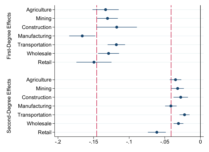
Figure A1: Heterogeneity of the Effects of Conflict on Trade by Firms’ Industry

Notes: The figure presents the heterogeneity estimates of the propagation estimates in Table 4 by firms’ industry identified through their SIC classification. The outcome is the monthly frequency of trade. The figure is constructed as follows. First, we estimate the coefficients on the interactions between the first- and second-degree-conflict-partner indicators and the industry indicators for the seven SIC industry categories composing more than 3% of the sample (i.e., whether at least one of the two trade partners in a link works in one of these industries). Next, we linearly add the baseline and the heterogeneity postconflict first-degree and second-degree coefficients and depict them with 95% confidence bands. All regressions include establishment-pair-direction and year-month fixed effects. All other specification details in the notes to Table 4 apply.

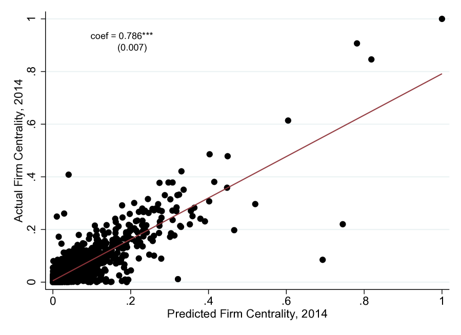
Figure A2: Relationship between Actual and Predicted Firm Centrality

Notes: This figure plots firm centrality in the 2014 production network with respect to predicted firm centrality estimated based on their network position in the modified 2013 production network without Crimea and the conflict areas in Donbas.

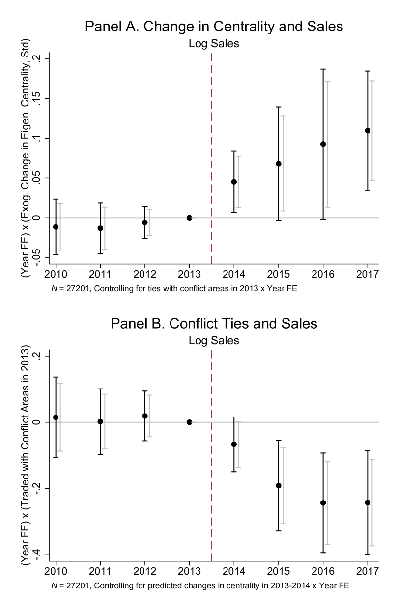
Figure A3: Conflict-Induced Change in Network Centrality and Sales:
Controlling for Ties to Conflict

Notes: This figure displays the results of estimating equation (4) and explores whether the baseline estimates for exogenous changes in firm centrality presented in Figure 3 and Section 7 are driven by the firm’s prior trade ties with the conflict areas. Panel A displays the results for the exogenous change in eigenvector centrality between 2013 and 2014 as the interaction variable, standardized to have zero mean and standard deviation of one. Panel B displays the results for any trade ties with conflict areas in 2013 as the interaction variable. The outcome variable is the logarithm of sales. Black bars represent 95% confidence intervals, gray bars represent 90% confidence intervals. Standard errors are clustered at the firm level.

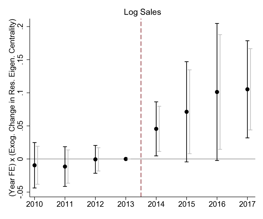
Figure A4: Conflict-Induced Change in Network Centrality and Sales:
Residualizing Firm Characteristics

Notes: This figure explores whether the baseline estimates for changes in firm centrality presented in Figure 3 and Section 7 are driven by firm characteristics. We calculate the residual change in centrality as the residual after regressing the change in centrality without adjustment on: an indicator whether a firm traded with someone in the conflict areas, the share of its transactions with the conflict areas, the share of its total sales with the conflict areas, the total weight of a firm’s partners’ trade with the conflict areas (i.e., through second-degree connections), as well as firm’s log sales and log profits in 2013. The obtained residuals are then used as a measure of exogenous change in centrality in equation (3). The outcome variable is the logarithm of sales. Black bars represent 95% confidence intervals, gray bars represent 90% confidence intervals. Standard errors are clustered at the firm level.

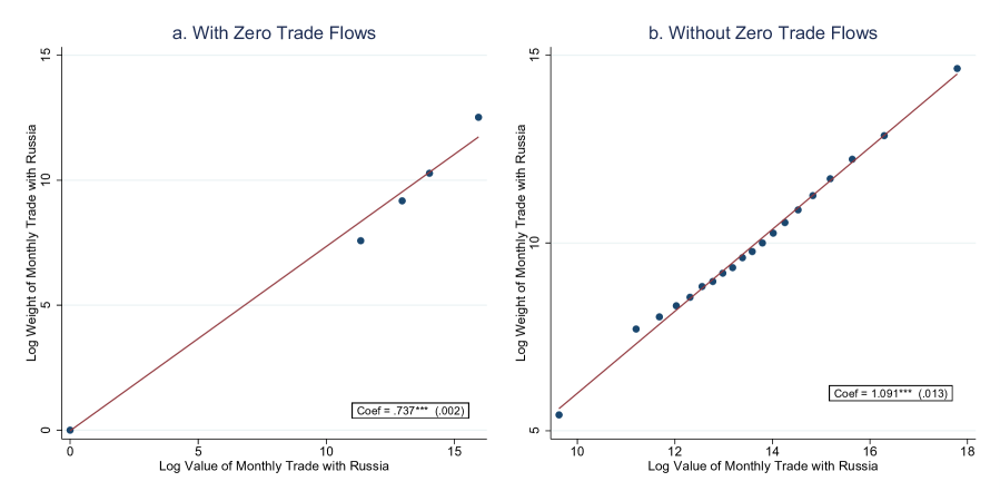
Figure A5: Correlation Between Total Weight and Value of Monthly Trade Flows Between Ukrainian Firms and Russia

Notes: This figure displays the binned scatter plots of the total weight and value of monthly trade flows between Ukrainian firms and Russia. Panel A includes the instances of zero monthly trade and Panel B excludes such instances. The figure relies on Ukrainian customs data from Korovkin and Makarin (2022). The time period is January 2013 through December 2016. Standard errors are clustered at the firm level. * p$<$0.05, ** p$<$0.01, *** p$<$0.001.

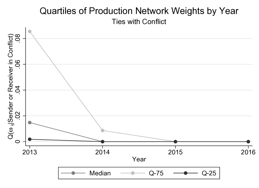
Figure A6: Production Network Weights for Trade with Conflict Areas

Notes: This figure displays the quartiles of the distribution of production network weights (elements) corresponding to trade with DPR, LPR, and Crimea. Q-25 refers to the first quartile or the 25th percentile and Q-75 refers to the third quartile or the 75th percentile of the element. distribution.

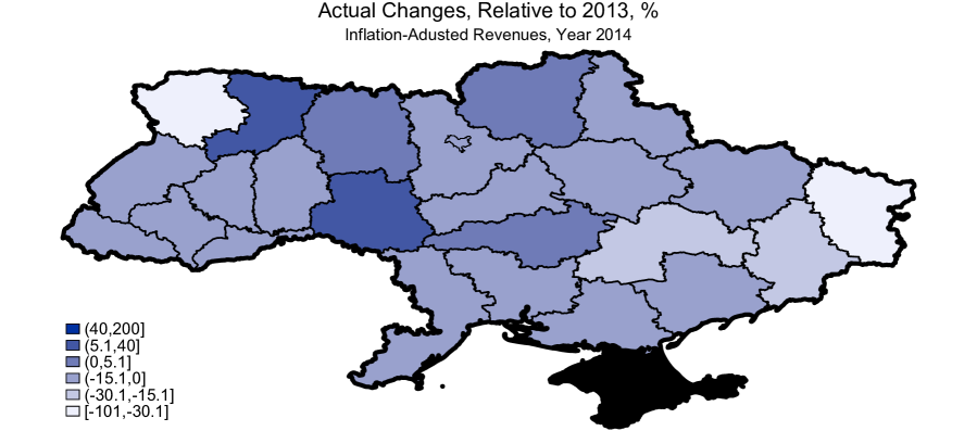
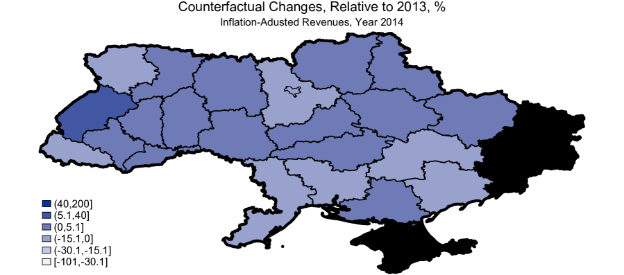
Figure A7: Network-Adjustment Counterfactual and Actual Changes, Province-Level

Notes: The graph depicts the evolution of raw and counterfactual revenues by Ukrainian provinces (oblasts). Darker colors indicate more positive changes. Black areas are either annexed or affected by the conflict. We use the black areas to estimate the outside demand $\bm{\xi}$, but not in reporting the counterfactuals. The top map displays the observed province-level changes of aggregate firm revenues in 2013–2014. The bottom map shows the changes in counterfactual revenues $\bm{r}$ for a given input-output matrix $\mathbb{\Omega}$ and outside demand $\bm{\xi}$ such that $\bm{r}(\bm{\xi},\mathbb{\Omega}):=[\mathbb{I}-(1-\alpha)\mathbb{\Omega}]^{-1}\bm{\xi}$, fixing outside demand at the 2013 level and using the actual 2014 railway trade matrix between provinces, $\mathbb{\Omega^{2014}_{province}}$.

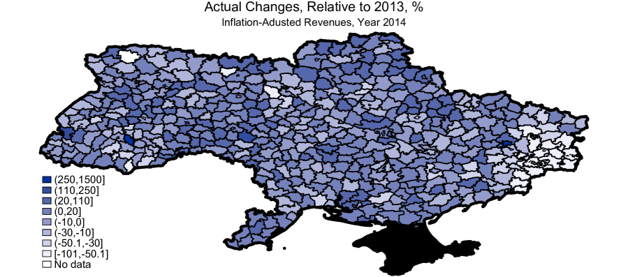
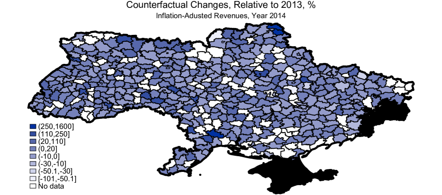
Figure A8: Network-Adjustment Counterfactual and Actual Changes, District-Level

Notes: The graph depicts the evolution of raw and counterfactual revenues by Ukrainian districts (rayons). Darker colors indicate more positive changes. Black areas are either annexed or affected by the conflict. We use the black areas to estimate the outside demand $\bm{\xi}$, but not in reporting the counterfactuals. Missing data at the district level are depicted in white: those districts do not have railways. The top map displays the observed changes of aggregate firm revenues in 2013–2014. The bottom map shows the changes in counterfactual revenues $\bm{r}$ for a given input-output matrix $\mathbb{\Omega}$ and outside demand $\bm{\xi}$ such that $\bm{r}(\bm{\xi},\mathbb{\Omega}):=[\mathbb{I}-(1-\alpha)\mathbb{\Omega}]^{-1}\bm{\xi}$, fixing the outside demand at the 2013 level and using the actual 2014 railway trade matrix between districts, $\mathbb{\Omega^{2014}_{district}}$.

Appendix B: Definitions of Centrality

To calculate degree centrality, we take an adjacency matrix $G=(g_{i,j})$, where $g_{i,j}$ is $1$ if firms $i$ and $j$ are linked and zero otherwise and define degree centrality for firms as a vector $C_{d}(G)$, where each entry is $C_{di}=\sum_{j=1}^{N}g_{ij}$. To define indegree and outdegree centrality, we replace $G$ with $G^{o}$ (and $G^{i}$), where $g_{i,j}$ is $1$ only if firm $i$ was selling (buying) to (from) firm $j$.

Betweenness centrality is a vector $C_{b}(G)$ where the $i$ entry is $C_{bi}=\sum_{k\neq j:i\{k,j\}}P_{i}(k,j)/P(k,j)$, $P(k,j)$ is the total number of shortest paths from $k$ to $j$, and $P_{i}(k,j)$ is the number of those paths that pass through $i$ without $i$ being an endpoint.

We define eigenvector centrality, $C_{e}(G)$, from the matrix equation: λC_e(G) = G C_e(G), where $\lambda$ is an eigenvalue corresponding to eigenvector $C_{e}(G)$. Following the consensus, we take the eigenvector associated with the largest eigenvalue.

Appendix C: Model Derivations

We focus on the problem of the firm in this economy and derive the equilibrium conditions of interest from it:

$$\max_{\{x_{ji},l_{i}\}}\Big{\{}p_{i}x_{i}-wl_{i}-\sum_{j=1}^{n}x_{ji}p_{j}\Big{\}},\text{ given }$$

$$x_{i}=(z_{i}l_{i})^{\alpha}\Big{(}\sum_{j=1}^{n}a_{ji}^{1/\sigma}x_{ji}^{(\sigma-1)/\sigma}\Big{)}^{\frac{\sigma}{\sigma-1}(1-\alpha)}.$$

Deriving the first-order conditions for $l_{i}$ and $x_{ji}$ and multiplying by $l_{i}$ and $x_{ji}$, one gets the following system:

$$\begin{cases}wl_{i}=\alpha p_{i}x_{i},\\ (1-\alpha)p_{i}x_{i}\cdot\frac{a_{ji}^{1/\sigma}x_{ji}^{\frac{\sigma-1}{\sigma}}}{\sum_{k=1}^{n}a_{ki}^{1/\sigma}x_{ki}^{\frac{\sigma-1}{\sigma}}}=p_{j}x_{ji}.\end{cases}$$

Taking the ratio of the first-order conditions for two inputs $j$ and $m$ one gets

$$\frac{(a_{ji}/x_{ji})^{1/\sigma}}{(a_{mi}/x_{mi})^{1/\sigma}}=\frac{p_{j}}{p_{m}},$$

rearranging and solving for $x_{ji}$, one gets,

$$x_{ji}=\frac{a_{ji}}{p_{j}^{\sigma}}\frac{\sum_{m}p_{m}x_{mi}}{\sum_{m}p_{m}^{1-\sigma}a_{mi}}.$$

Next we use market clearing condition $x_{i}=\sum_{j=1}^{n}x_{ji}+c_{i}$ to derive further the equilibrium revenue of each firm: r_i = p_i x_i = ∑_j=1^n p_i x_ij + p_i c_i Then, expressing $x_{ij}$ from the first-order condition, and plugging it back into $r_{i}$, we get,

$$r_{i}=\sum_{j=1}^{n}p_{i}\frac{(1-\alpha)p_{j}x_{j}}{p_{i}}\frac{a_{ij}^{1/\sigma}x_{ij}^{\frac{\sigma-1}{\sigma}}}{\sum_{k=1}^{n}a_{kj}^{1/\sigma}x_{kj}^{\frac{\sigma-1}{\sigma}}}=$$

$$(1-\alpha)\sum_{j=1}^{n}\underbrace{\frac{a_{ij}/p_{i}^{1-\sigma}(\mathbf{a})}{\sum_{m}a_{mj}/p_{m}^{1-\sigma}(\mathbf{a})}}_{\text{I-O weight }\omega_{ij}(\mathbf{a})}\cdot r_{j}+\underbrace{p_{i}c_{i}}_{\text{outside demand }\bm{\xi}}.$$

References

- Abadie and Gardeazabal (2003) Abadie, A. and J. Gardeazabal (2003). The Economic Costs of Conflict: A Case Study of the Basque Country. American Economic Review 93(1), 113–132.
- Acemoglu and Azar (2020) Acemoglu, D. and P. D. Azar (2020). Endogenous production networks. Econometrica 88(1), 33–82.
- Acemoglu et al. (2012) Acemoglu, D., V. M. Carvalho, A. Ozdaglar, and A. Tahbaz-Salehi (2012). The network origins of aggregate fluctuations. Econometrica 80(5), 1977–2016.
- Acemoglu et al. (2017) Acemoglu, D., A. Ozdaglar, and A. Tahbaz-Salehi (2017). Microeconomic origins of macroeconomic tail risks. American Economic Review 107(1), 54–108.
- Alesina et al. (1996) Alesina, A., S. Özler, N. Roubini, and P. Swagel (1996). Political instability and economic growth. Journal of Economic growth 1(2), 189–211.
- Amodio et al. (2021) Amodio, F., L. Baccini, and M. Di Maio (2021). Security, trade, and political violence. Journal of the European Economic Association 19(1), 1–37.
- Amodio and Di Maio (2018) Amodio, F. and M. Di Maio (2018). Making do with what you have: Conflict, input misallocation and firm performance. The Economic Journal 128(615), 2559–2612.
- Bahgat et al. (2018) Bahgat, K., K. Dupuy, G. Østby, S. A. Rustad, H. Strand, and T. Wig (2018). Children and Armed Conflict: What Existing Data Can Tell Us. Technical report, PRIO.
- Baqaee (2018) Baqaee, D. R. (2018). Cascading failures in production networks. Econometrica 86(5), 1819–1838.
- Baqaee and Farhi (2019) Baqaee, D. R. and E. Farhi (2019). The macroeconomic impact of microeconomic shocks: beyond hulten’s theorem. Econometrica 87(4), 1155–1203.
- Baqaee and Farhi (2020) Baqaee, D. R. and E. Farhi (2020). Productivity and misallocation in general equilibrium. The Quarterly Journal of Economics 135(1), 105–163.
- Barrot and Sauvagnat (2016) Barrot, J.-N. and J. Sauvagnat (2016). Input specificity and the propagation of idiosyncratic shocks in production networks. The Quarterly Journal of Economics 131(3), 1543–1592.
- Bigio and La’O (2016) Bigio, S. and J. La’O (2016). Financial frictions in production networks. Technical report, National Bureau of Economic Research.
- Blattman and Miguel (2010) Blattman, C. and E. Miguel (2010). Civil War. Journal of Economic Literature, 3–57.
- Boehm et al. (2019) Boehm, C. E., A. Flaaen, and N. Pandalai-Nayar (2019). Input linkages and the transmission of shocks: Firm-level evidence from the 2011 Tōhoku earthquake. Review of Economics and Statistics 101(1), 60–75.
- Borusyak and Hull (2020) Borusyak, K. and P. Hull (2020). Non-random exposure to natural experiments: Theory and applications. NBER Working Paper 27845.
- Carvalho et al. (2021) Carvalho, V. M., M. Nirei, Y. U. Saito, and A. Tahbaz-Salehi (2021). Supply Chain Disruptions: Evidence from the Great East Japan Earthquake. The Quarterly Journal of Economics 136(2), 1255–1321.
- Carvalho and Tahbaz-Salehi (2019) Carvalho, V. M. and A. Tahbaz-Salehi (2019). Production networks: A primer. Annual Review of Economics 11, 635–663.
- Cerra and Saxena (2008) Cerra, V. and S. C. Saxena (2008). Growth dynamics: the myth of economic recovery. American Economic Review 98(1), 439–57.
- Chaney (2008) Chaney, T. (2008). Distorted gravity: the intensive and extensive margins of international trade. American Economic Review 98(4), 1707–21.
- Couttenier et al. (2022) Couttenier, M., N. Monnet, and L. Piemontese (2022). The economic costs of conflict: A production network approach.
- Del Prete et al. (2021) Del Prete, D., M. Di Maio, and A. Rahman (2021). Firms amid conflict: Performance, production inputs, and market competition. Available at SSRN.
- Dell and Querubin (2018) Dell, M. and P. Querubin (2018). Nation Building through Foreign Intervention: Evidence from Discontinuities in Military Strategies. Quarterly Journal of Economics.
- Donaldson (2018) Donaldson, D. (2018). Railroads of the Raj: Estimating the Impact of Transportation Infrastructure. American Economic Review 108(4-5), 899–934.
- Donaldson and Hornbeck (2016) Donaldson, D. and R. Hornbeck (2016). Railroads and American Economic Growth: A “Market Access” Approach. The Quarterly Journal of Economics 131(2), 799–858.
- Esteban and Ray (1999) Esteban, J. and D. Ray (1999). Conflict and distribution. Journal of Economic Theory 87(2), 379–415.
- Fearon and Laitin (2003) Fearon, J. D. and D. D. Laitin (2003). Ethnicity, insurgency, and civil war. American political science review 97(1), 75–90.
- Ferrari (2019) Ferrari, A. (2019). Global Value Chains and the Business Cycle. Available at SSRN 3249434.
- Fisman et al. (2020) Fisman, R., A. Sarkar, J. Skrastins, and V. Vig (2020). Experience of communal conflicts and intergroup lending. Journal of Political Economy 128(9), 3346–3375.
- Guidolin and La Ferrara (2007) Guidolin, M. and E. La Ferrara (2007). Diamonds are Forever, Wars are Not: Is Conflict Bad for Private Firms? American Economic Review 97(5), 1978–1993.
- Guiso et al. (2009) Guiso, L., P. Sapienza, and L. Zingales (2009). Cultural Biases in Economic Exchange? The Quarterly Journal of Economics 124(3), 1095–1131.
- Hjort (2014) Hjort, J. (2014). Ethnic Divisions and Production in Firms. The Quarterly Journal of Economics 129(4), 1899–1946.
- Kalemli-Ozcan et al. (2015) Kalemli-Ozcan, S., B. Sorensen, C. Villegas-Sanchez, V. Volosovych, and S. Yesiltas (2015). How to Construct Nationally Representative Firm Level Data from the ORBIS Global Database. Technical report, National Bureau of Economic Research.
- Korovkin and Makarin (2022) Korovkin, V. and A. Makarin (2022). Conflict and Inter-Group Trade: Evidence from the 2014 Russia-Ukraine Crisis. American Economic Review.
- Ksoll et al. (2021) Ksoll, C., R. Macchiavello, and A. Morjaria (2021). Electoral Violence and Supply Chain Disruptions in Kenya’s Floriculture Industry. Review of Economics and Statistics, forthcoming.
- Liu and Tsyvinski (2020) Liu, E. and A. Tsyvinski (2020). Dynamical structure and spectral properties of input-output networks. Technical report, National Bureau of Economic Research.
- Long Jr and Plosser (1983) Long Jr, J. B. and C. I. Plosser (1983). Real business cycles. Journal of political Economy 91(1), 39–69.
- MacKinnon and Magee (1990) MacKinnon, J. G. and L. Magee (1990). Transforming the Dependent Variable in Regression Models. International Economic Review, 315–339.
- Magerman et al. (2016) Magerman, G., K. De Bruyne, E. Dhyne, and J. Van Hove (2016). Heterogeneous firms and the micro origins of aggregate fluctuations. Technical report, NBB Working Paper.
- Markevich et al. (2021) Markevich, A., N. Naumenko, and N. Qian (2021). The political-economic causes of the soviet great famine, 1932–33. Technical report, National Bureau of Economic Research.
- Martin et al. (2008a) Martin, P., T. Mayer, and M. Thoenig (2008a). Civil Wars and International Trade. Journal of the European Economic Association 6(2-3), 541–550.
- Martin et al. (2008b) Martin, P., T. Mayer, and M. Thoenig (2008b). Make trade not war? The Review of Economic Studies 75(3), 865–900.
- Melitz (2003) Melitz, M. J. (2003). The Impact of Trade on Intra-industry Reallocations and Aggregate Industry Productivity. Econometrica 71(6), 1695–1725.
- Montalvo and Reynal-Querol (2005) Montalvo, J. G. and M. Reynal-Querol (2005). Ethnic polarization, potential conflict, and civil wars. American economic review 95(3), 796–816.
- Nunn and Qian (2014) Nunn, N. and N. Qian (2014). Us food aid and civil conflict. American Economic Review 104(6), 1630–66.
- OSHA (2014) OSHA (2014). Standard Industrial Classification (SIC) Manual. Occupational Safety and Health Administration, United States Department of Labor.
- Rohner and Thoenig (2021) Rohner, D. and M. Thoenig (2021). The Elusive Peace Dividend of Development Policy: From War Traps to Macro Complementarities. Annual Review of Economics 13(1), 111–131.
- Rohner et al. (2013) Rohner, D., M. Thoenig, and F. Zilibotti (2013). War Signals: A Theory of Trade, Trust, and Conflict. Review of Economic Studies 80(3), 1114–1147.
- SPARK-Interfax (2017) SPARK-Interfax (2010–2017). Spark-interfax database. https://spark-interfax.com/.
- Treisman (2018) Treisman, D. (2018). The New Autocracy: Information, Politics, and Policy in Putin’s Russia. Brookings Institution Press.
- Utar (2018) Utar, H. (2018). Firms and Labor in Times of Violence: Evidence from the Mexican Drug War.