Decay: A Monte Carlo library for the decay of a particle with ROOT compatibility

Abstract

Recently, there is a need for a general-purpose event generator of decays of an elementary particle or a hadron to a state of higher multiplicity ($N>2$) that is simple to use and universal. We present the structure of such a library to produce generators that generate kinematics of decay processes and can be used to integrate any matrix element squared over phase space of this decay. Some test examples are presented, and results are compared with results known from the literature. As one of examples we consider the Standard Model Higgs boson decay into four leptons. The generators discussed here are compatible with the ROOT interface.

I Introduction

In modern high energy physics or hadronic physics, the prime role is played by complex multiprocess Monte Carlo generators. One example of such a versatile tool is Pythia Sjostrand:2014zea ; Sjostrand:2006za .

However, apart from beam colliding experiments, there are various experiments (e.g., Aaltonen:2015uva ; Adam:2020sap ; Sirunyan:2020cmr ; Sikora_PhD_thesis ) that measure decaying unstable particle products. In many cases, there are specific generators for such processes, with specific matrix elements and kinematics tuned for the particular decay.

However, in some theoretical investigation, there is a need for a simple yet versatile generator for prototyping new theories or to understand mechanism of decays of mesons or baryons. Good examples are exotic decays of conventional mesons, decays of glueballs or tetraquarks. One typical choice is the GENBOD code James:1968 which uses the Raubold and Lynch algorithm. It is delivered in ROOT package ROOT as TGenPhaseSpace class. There are some inconveniences in the use of this generator. The events are weighted, and it requires some work to integrate some expression over a phase space and generate events. Moreover, some additional tools must be added to provide adaptive Monte Carlo integration/simulation.

These inconveniences were present during our theoretical investigations of the phenomenology of decaying processes Lebiedowicz:2016zka ; Lebiedowicz:2019jru , where the $1\to 4$ decay processes were simulated from the $1\to 2$ process with a corresponding spectral functions. This motivated us to constuct a new, more powerful Monte Carlo generators for decays. They should be compatible with ROOT software and, due to adaptivity, can handle with integrands that have ’small’ support in the Lorentz Invariant Phase Space (LIPS). These tools are based on some elements from our previous exclusive MC generator GenEx Kycia:2014hea ; Kycia:2017ota . The essential requirement in designing these tools is that the interface should be fully compatible with ROOT generator TGenPhaseSpace and use effectively other ROOT components.

One of the application of these tools will be to use them in central exclusive diffractive production of $\pi^{+}\pi^{-}\pi^{+}\pi^{-}$ Lebiedowicz:2016zka ; Kycia:2017iij and $K^{+}K^{-}K^{+}K^{-}$ Lebiedowicz:2019jru in proton-proton collisions that proceeds via resonances. These processes are under recent experimental studies at RHIC and LHC Adam:2020sap ; Sirunyan:2020cmr ; Sikora_PhD_thesis .

Another application is their use in search of hypothetical resonances of new physics and study their properties, e.g., in the four-lepton channel Aaboud:2017rel ; Aad:2020fpj . The $H\to ZZ\to 4\ell$ channel, as compared to other final states, has the advantage of being experimentally clean and, for this reason, is considered the “golden” channel to explore the possible existence of a heavy Higgs resonance. As an example, we consider the decay $H\to ZZ\to 4\ell$ of spin 0 Higgs boson with mass $M_{H}=125.1$ GeV.

The paper is organized as follows: In the next section, implementation details and usage of the library will be presented. The package also contains three generators for decays with two, three, and four particles in the final states. The physical process of these kinds for testing purposes were described in the second part of the paper. These are the application of $4$-Fermi theory to $\mu$ decay and the Standard Model Higgs boson decay to four leptons.

II Implementation details

II.1 General requirements and running Decay

The requirements for running the software are:

• ROOT library ROOT - the set of generators integrates with this library and uses many of its components.

• $C/C++$ compiler - the default compiler is the one with GNU GCC collection GCC .

• GNU MAKE GNUMAKE - examples are provided with fully functional Makefiles.

• Doxygen Doxygen - for generating documentation from the code.

The examples are supplied with Makefile with the following commands defined:

• make run - compiles and runs the example.

• make clean - cleans executables.

• make cleanest - cleans executables and results of simulation.

• make Generate-doc - generates documentation in pdf and LaTeX file using Doxygen.

II.2 How to install Decay

The library and examples can be downloaded from the repository GitHub:2020 . The repository is split into two directories:

• Library - contains header files and implementations of library. These files can be placed inside the user directory or placed in common place for compiler.

• Examples - contains three examples described below in details. They illustrate the use of files from library in a real-life applications:

  • 2DDecay - decay of a central blob into two particles; see Section III.1 for details.

  • 4Fermi - $\mu\to\nu_{\mu}e\bar{\nu}_{e}$ decay in 4-Fermi phenomenological theory Schwartz:2013pla ; see Section III.2 for details.

  • H4 - contains two models of $H$ decay to four leptons described below; see Section III.3 for details.

In order to use the content of Library directory you have to write your own C++ main.cxx file that includes specific files from the directory. A detailed description is provided below.

It is however advised to experiment with specific examples beforehand. They are stand-alone programs that are using Decay library from Library directory. The examples can be used as a starting point for writing the generator for a new process economically.

Each example is supplied with Makefile that simplifies process of compiling and running. The commands to run the examples are as follows:

• make run - compiles and runs the example.

• make clean - cleans executables.

• make cleanest - cleans executables and results of simulation.

• make Generate-doc - generates documentation in pdf and LaTeX file using Doxygen.

II.3 Input

The examples require no specific input, and all specific parameters and matrix elements of physical models are present in corresponding main.cxx files.

II.4 Output

Each generator in the discussed here examples generates four-vectors of particles from the decay. They are saved in the file events.txt on disk and some control plots of rapidity and invariant mass in eps/pdf files, and, in addition, the file histograms.root to create a histograms in ROOT. These are standard ways how to deal with events using straightforward approach known from the ROOT package. All the logic is contained in main.cxx file.

II.5 Two modes of using examples of Decay

The presented here examples of Decay package can be used in two distinct ways:

• First events are generated according to phase-space distributions. Then the events are weighted by the square of the matrix element ${\cal M}_{1\to n}$ for the $1\to n$ decay prepared by the user outside of the generator in a separate program. This option may be easier for the user but difficult for controlling accuracy.

• The matrix element squared for the decay is inserted directly into the generator itself. This option may be more optimal as far as efficiency and accuracy are considered.

II.6 Structure of classes

In this section, the structure of the system of generators will be presented. This description is related to the files in Library directory and is aimed at users who want to write the generator based on this library from scratch.

The library uses the modified TDecay class from previous generator for exclusive processes GenEx Kycia:2014hea ; Kycia:2017ota that is based on the original GENBOD algorithm James:1968 . The interface is based on TGenPhaseSpace class from ROOT for compatibility. The difference is that

• It requires (pseudo)random numbers to generate an event. This is needed to connect this generator with an external system that feeds this numbers, e.g., adaptive sampling as described below.

• It returns the volume of the Lorentz Invariant Phase Space (LIPS) James:1968 ; Hagedorn:1964 ; Pilkuhn:1967 ; Schwartz:2013pla

  $$d^{(n)}{\rm LIPS}=d{\rm LIPS}\left(P\rightarrow\sum_{i=1}^{n}p_{i}\right)=(2\pi)^{4}\delta^{(4)}\left(P-\sum_{i=1}^{n}p_{i}\right)\prod_{i=1}^{n}\frac{d^{3}p_{i}}{(2\pi)^{3}2E_{i}}\,,$$ (1)

  where $P$ is the 4-momentum of decaying particle, $p_{i}$ are 4-momenta of the decay products and $E_{i}$ their energies.

This class follows the general interface described in the following subsection.

II.7 Interface description

In this subsection, we describe the interface of the discussed decay generators. The interface is derived from the standard ROOT generator TGenPhaseSpace to make it compatible with this package. The interface is enclosed in the abstract class TGenInterface that is presented in Fig. 1.

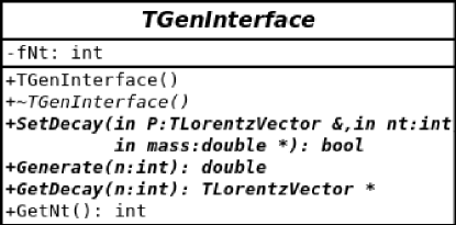
Figure 1: Interface for generators.

The description of methods is as follows:

• SetDecay(TLorentzVector &P, Int_t nt, const Double_t *mass) - set decay configuration. The initial 4-momentum of a particle is $P$, $nt$ is the number of final state particles, and $mass$ is an array of masses of final particles. This is the first method that should be called before generating an event. It returns true when configuration is allowed and false otherwise.

• Generate(void) generates an event and returns the weight of this event. It should be called after the configuration is set.

• GetDecay(Int_t n) returns the $n$-th product of the decay as a 4-vector.

When using object that realizes above interface, the sequence of calls should as follows:

1. SetDecay(...)

2. In the loop:

   1. Generate(...)

   2. GetDecay(...)

This mimic the sequence of calls from well known TGenPhaseSpace class of ROOT for compatibility.

This interface is implemented in the following generators.

II.8 TDecay

The TDeacy class contains specialization of the TGenDecay specific methods with specialization. The method Generate (std::queue< double > &rnd) takes the queue rnd of $3n-4$ random numbers needed for generation of events. The weight returned by this method is precisely (1).

This class is the backbone of more advanced generators described below.

II.9 TGenDecay

Wrapping of TDeacy with the uniform random number generator is TGenDecay. Its class diagram is presented in Fig. 2.

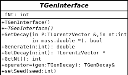
Figure 2: The diagram of class TGenDecay.

Apart of the methods from the TGenInterface, there is an additional method setSeed(...), which sets the seed for internal pseudorandom number generator.

The inheritance diagram is presented in Fig. 3.

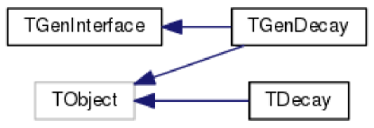
Figure 3: Inheritance diagram for TGenDecay.

The inheritance from TObject from the ROOT class is for compatibility.

The typical use of this generator is as follows:

• TGenDecay generator; - makes an instance of the generator;

• generator.SetDecay(P, nt, mass); - sets the decay configuration;

• In the loop over events ($N$-times):

  • w = generator.Generate(); - makes an event and remembers the volume of the phase space in double w; Call the LIPS weight for $i$-th event $w_{i}$.

  • pfi = *(generator.GetDecay( i )); - get the 4-momentum of $i$-th particle; It can be done for all particles needed to compute integrand.

  • Computes the integrand $I_{i}$ for the $i$-th event.

Then by the standard Monte Carlo reasoning James:1968 the integral is

$$\int I(p_{1},\ldots,p_{nt})\,d{\rm LIPS}\approx<I>\pm\sigma,$$ (2)

where

$$<I>=\frac{1}{N}\sum_{i=1}^{N}I_{i}w_{i},$$ (3)

and the error estimate is

$$\sigma=(<I>^{2}-<I^{2}>)\sqrt{N},$$ (4)

where

$$<I^{2}>=\frac{1}{N}\sum_{i=1}^{N}w_{i}I_{i}^{2}.$$ (5)

The class TGenDecay is useful for symmetric decay. Therefore it can be used for integrating matrix element that is not aspherical since then the effectiveness can be low, as it was shown for TDecay in Kycia:2017ota ; Kycia:2014hea . If this is the case, then a more advanced decay generator described in the next section is more relevant.

II.10 Adaptive decay with TGenFoamDecay

There are cases where a simple approach described above is insufficient. The first one is when the integrand has the support, which is small in the LIPS region over which we integrate. This includes the integrands, which have strong ’non-spherical’ cuts on momenta and energies of decay products. In this case, one can try to integrate over LIPS using the adaptive Monte Carlo procedure. There are two common general-purpose MC integrators VEGAS Lepage:1977sw ; Ohl:1998jn ; Lepage:2020tgj and FOAM Jadach:2002kn . Merging of the TDecay and FOAM algorithm is made in TGenFoamDecay class.

The class diagram is presented in Fig. 4.

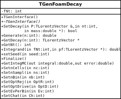
Figure 4: Class diagram for TGenFoamDecay.

The difference between TGenDecay and TGenFoamDecay is due to FOAM content and facilitate adaptive integration. The following methods are new compared to the interface TGenInterface:

• In the SetDecay(...) method, the initialization of FOAM decay is made.

• Double_t Integrand( int fNt, TLorentzVector* pf ) - is a virtual method that fixes integrand that FOAM integrates over LIPS. In the method fNt is the number of particles, and pf - momenta of the decay products. In this class it returns $1.0$ and can be changed when the user makes a new class that inherits from TGenFoamDecay, as it will be explained below.

• Finalize( void ) - the method that makes finalization of FOAM and prints the integral and its error on the terminal.

• GetIntegMC(Double_t & integral, Double_t & error) - the method that allows to extract the integral and its error from the FOAM integrator inside TGenFoamDecay.

• The methods Set... are setting parameters of FOAM integrator Jadach:2002kn . Default values are good for most standard applications, however, if it is not the case these parameters should be set before SetDecay(...) is called. Some practical hints are as follows:

  • If the matrix element has ’small’ support in LIPS and the integral is small, then the nCells and nSampl should be increased.

  • By default, TGenFoamDecay generates the events with weight $1.0$ since OptRej=1. However, if one prefers weighted events, then one should set OptRej=0.

Use of TGenFoamDecay in a specific decay with a specific matrix element of reaction is made by deriving a new class from TGenFoamDecay and redefining virtual function Integrand(..). For example, below, the specific Generator class was derived and the Integrand method was specified.

class Generator: public TGenFoamDecay
{
Double_t Integrand( int fNt, TLorentzVector * pf );
};

Double_t Generator::Integrand( int fNt, TLorentzVector * pf )
{
double integrand = 1.0; //Here put your integrand instead of 1.0
return integrand;Ψ
};Ψ

Inheritance diagram is presented in Fig. 5. It shows that TGenFoamDecay implements TGenInterface interface and at the same time is FOAM integrand class TFoamIntegrand.

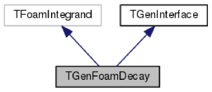
Figure 5: Inheritance diagram for TGenFoamDecay.

In the next section, some simple and useful applications and tests of the discussed generator will be described.

III Tests

The detailed test of TDecay was presented in Kycia:2017ota . We present tests of the use of the full generators in examples of decays into 2, 3, and 4 final state particles. Examples that realize these test are contained in Examples directory of GitHub:2020 .

III.1 Two particle decay

In the case of a two-particle final state, the integral over the whole phase space is known in the closed form Hagedorn:1964 ; Pilkuhn:1967 , namely, in the center of mass of particle $a$ we have

$$R_{2}(a\rightarrow b+c) = \int\frac{d^{3}p_{b}d^{3}p_{c}}{(2\pi)^{3}2E_{b}(2\pi)^{3}2E_{c}}(2\pi)^{4}\delta^{(4)}(P_{a}-(p_{b}+p_{c}))$$ (6)

$$= \frac{\pi}{2m_{a}^{2}(2\pi)^{2}}\sqrt{(m_{a}^{2}-(m_{b}+m_{c})^{2})(m_{a}^{2}-(m_{b}-m_{c})^{2})}\,.$$

For a test we considered a decay of a hypothetical decay of particles $m_{a}=m_{\mu}$ into $m_{b}=m_{c}=m_{e}$. This can serve as a precise test since the formula for the decay is exact in this case.

III.2 Three particle decay

In the 4-Fermi theory Schwartz:2013pla , which is an effective theory of weak interactions, the decay $\mu\to e\nu_{\mu}\bar{\nu}_{e}$ is given by the simple matrix element Schwartz:2013pla

$$|{\cal M}|^{2}=32\,G_{F}^{2}(m_{\mu}^{2}-2m_{\mu}E_{\bar{\nu}_{e}})m_{\mu}E_{\bar{\nu}_{e}}\,,$$ (7)

where the Fermi coupling constant $G_{F}=1.166379\times 10^{-5}$ GeV^-2 makes the energy scale of the usefulness of this non-renormalizable theory, $m_{\mu}$ is the mass of muon, $E_{\bar{\nu}_{e}}$ is the energy of the outgoing electron antineutrino $\bar{\nu}_{e}$, and the masses of neutrinos are negligible ($m_{\nu_{\mu}}=m_{\bar{\nu}_{e}}=0$). The decay width is given by the standard formula

$$\Gamma(\mu\to e\nu_{\mu}\bar{\nu}_{e})=\frac{1}{2m_{\mu}}\int|{\cal M}|^{2}d^{(3)}{\rm LIPS}\,,$$ (8)

which can be calculated analytically to Schwartz:2013pla

$$\Gamma(\mu\to e\nu_{\mu}\bar{\nu}_{e})=\frac{G_{F}^{2}m_{\mu}^{5}}{192\pi^{3}}\,.$$ (9)

This makes a perfect testbed for the generator.

In case of use TGenFoamDecay class, we derive Generator class that redefines integrand by (8), namely,

class Generator: public TGenFoamDecay
{
Double_t Integrand( int fNt, TLorentzVector * pf );Ψ
};

Double_t Generator::Integrand( int fNt, TLorentzVector * pf )
{
const double G = 1.166e-5;
const double mmu = 0.1057;
double M2 = 32.0*G*G*( mmu*mmu-2.0*mmu*pf[2].E() ) * mmu*pf[2].E();
double corr = 1.0/(2.0*mmu) ;
return M2 * corr;Ψ
};Ψ

where the $\rm pf[2]$ is the TLorentzVector object that represents 4-momentum of $\bar{\nu}_{e}$, if we define the mass matrix in the following order mass = {$m_{e}$, $m_{\nu_{\mu}}$, $m_{\bar{\nu}_{e}}$}.

Table 2 presents the convergence of the Monte Carlo method using TGenDecay. It is the typical convergence with $\sim\frac{1}{\sqrt{N}}$ accuracy, where $N$ is statistics of events.

# events	$\Gamma_{n}$ [GeV]	$\mathinner{\!\left\lvert\Gamma_{n}-\Gamma_{\rm exact}\right\rvert}$ [GeV]
$10^{2}$	$2.9285\times 10^{-19}$	$8.465\times 10^{-21}$
$10^{4}$	$3.00344\times 10^{-19}$	$9.71\times 10^{-22}$
$10^{6}$	$3.01232\times 10^{-19}$	$8.3\times 10^{-23}$

Table 1: The value of $\Gamma_{n}$ (8) obtained by TGenDecay integration. The exact value (9) is $\Gamma_{\rm exact}=3.01315\times 10^{-19}$ GeV.

III.3 Four particle decay

In this subsection, we describe a test of the decay of the Standard Model Higgs boson into four leptons $H\rightarrow 4\ell$, which is of interest in precision tests of Higgs boson at the LHC and in future colliders.

The decay rate for $H\rightarrow 4\ell$ can be written as

$$\Gamma(H\to 4\ell)=\frac{1}{2M_{H}}\frac{1}{F}\int{\mathinner{\!\left\lvert{\cal M}_{H\to 4\ell}\right\rvert}^{2}}d^{(4)}{\rm LIPS}\;,$$ (10)

where $1/F$ is the identity factor of particles in the final state ($F=1$ for $e^{+}e^{-}\mu^{+}\mu^{-}$ and $F=4$ for $\mu^{+}\mu^{-}\mu^{+}\mu^{-}$).

III.3.1 The matrix element for $H\to 4\ell$ decay

Here we consider the decay amplitudes of the Higgs boson into four leptons in two processes.

For the decay

$$H(P)\to e^{+}(p_{1})\,e^{-}(p_{2})\,\mu^{+}(p_{3})\,\mu^{-}(p_{4})$$ (11)

via the intermediate $Z$ bosons, the amplitude reads

$${\cal M}_{H\to e^{+}e^{-}\mu^{+}\mu^{-}}=e^{3}\,g_{HZZ}$$

$$\qquad\times\frac{1}{(p_{1}+p_{2})^{2}-M_{Z}^{2}+iM_{Z}\Gamma_{Z}}\,\bar{u}_{s_{2}}(p_{2})[\gamma^{\mu}(g_{Z\ell\ell}^{+}\omega_{+}+g_{Z\ell\ell}^{-}\omega_{-})]v_{s_{1}}(p_{1})$$

$$\qquad\times\frac{1}{(p_{3}+p_{4})^{2}-M_{Z}^{2}+iM_{Z}\Gamma_{Z}}\,\bar{u}_{s_{4}}(p_{4})[\gamma_{\mu}(g_{Z\ell\ell}^{+}\omega_{+}+g_{Z\ell\ell}^{-}\omega_{-})]v_{s_{3}}(p_{3})\,,$$ (12)

where $u_{s}(p)$ and $v_{s}(p)$ are momentum-dependent Dirac spinors for a fermion and anti-fermion, respectively.

For the decay

$$H(P)\to\mu^{+}(p_{1})\,\mu^{-}(p_{2})\,\mu^{+}(p_{3})\,\mu^{-}(p_{4})$$ (13)

via the intermediate $Z$ bosons, the amplitude reads

$${\cal M}_{H\to\mu^{+}\mu^{-}\mu^{+}\mu^{-}}={\cal M}_{H\to\mu^{+}\mu^{-}\mu^{+}\mu^{-}}^{(1)}-{\cal M}_{H\to\mu^{+}\mu^{-}\mu^{+}\mu^{-}}^{(2)}$$ (14)

with ${\cal M}_{H\to\mu^{+}\mu^{-}\mu^{+}\mu^{-}}^{(1)}$ as (12) but with $m_{e}\to m_{\mu}$ in the spinor wave functions and

$${\cal M}^{(2)}_{H\to\mu^{+}\mu^{-}\mu^{+}\mu^{-}}=\left.{\cal M}^{(1)}_{H\to\mu^{+}\mu^{-}\mu^{+}\mu^{-}}\right|_{p_{1},s_{1}\leftrightarrow p_{3},s_{3}}\,.$$ (15)

Above

$$\omega_{\pm}=\frac{1}{2}\left(\mathbb{1}_{4\times 4}\pm\gamma_{5}\right)\,,\quad\mathbb{1}_{4\times 4}=\left(\begin{array}[]{cc}\mathbb{1}&\;\,0\\ 0&\;\,\mathbb{1}\\ \end{array}\right)\,,\quad\mathbb{1}=\left(\begin{array}[]{cc}1&\;\,0\\ 0&\;\,1\\ \end{array}\right)\,,$$ (20)

$\omega_{\pm}$ are the right- and left-handed chirality projectors, $\mathbb{1}$ is the identity matrix. In the Dirac-Pauli representation, the gamma matrices $\gamma^{\mu}$ ($\mu=0,1,2,3$) and $\gamma^{5}$ read

$$\gamma^{0}=\gamma_{0}=\left(\begin{array}[]{cc}\mathbb{1}&\;\,0\\ 0&\;\,-\mathbb{1}\\ \end{array}\right)\,,\quad\gamma^{k}=-\gamma_{k}=\left(\begin{array}[]{cc}0&\;\,\sigma_{k}\\ -\sigma_{k}&\;\,0\\ \end{array}\right)\,,$$ (25)

$$\gamma_{5}=\gamma^{5}=i\gamma^{0}\gamma^{1}\gamma^{2}\gamma^{3}=\left(\begin{array}[]{cc}0&\;\,\mathbb{1}\\ \mathbb{1}&\;\,0\\ \end{array}\right)\,.$$ (28)

In (25) $k$ runs from 1 to 3 and the $\sigma_{k}$ are Pauli matrices.

In the Born approximation the relevant coupling constants read [see Appendices A of Denner:1991kt ; Denner:1994xt ]:

$$g_{HZZ}=\frac{M_{W}}{c^{2}_{\rm W}s_{\rm W}}=\frac{M_{Z}}{c_{\rm W}s_{\rm W}}\,,$$ (29)

$$g_{Z\ell\ell}^{+}=-\frac{s_{\rm W}}{c_{\rm W}}Q_{\ell}\,,$$ (30)

$$g_{Z\ell\ell}^{-}=-\frac{s_{\rm W}}{c_{\rm W}}Q_{\ell}+\frac{I_{{\rm W},\ell}^{3}}{s_{\rm W}c_{\rm W}}\,.$$ (31)

Above $c_{\rm W}^{2}=1-s_{\rm W}^{2}=M_{W}^{2}/M_{Z}^{2}$, $Q_{\ell}=-1$, and $I_{{\rm W},\ell}^{3}=-1/2$.

The usual Dirac spinors for the fermion and anti-fermion with momentum $p$ and spin in the $\pm z$ direction for $s=\pm 1/2$ (spin “up” or “down”) are

$$u_{s}(p)=\sqrt{E+m_{\ell}}\left(\begin{array}[]{c}\chi_{s}^{(1)}\vspace{0.2cm}\\ \dfrac{\mbox{\boldmath$\sigma$}\cdot\mbox{\boldmath$p$}}{p^{0}+m_{\ell}}\,\chi_{s}^{(1)}\\ \end{array}\right)\,,$$ (34)

$$v_{s}(p)=\sqrt{E+m_{\ell}}\left(\begin{array}[]{c}\dfrac{\mbox{\boldmath$\sigma$}\cdot\mbox{\boldmath$p$}}{p^{0}+m_{\ell}}\,\chi_{s}^{(2)}\vspace{0.2cm}\\ \chi_{s}^{(2)}\\ \end{array}\right)\,,$$ (37)

where $E=\sqrt{|\mbox{\boldmath$p$}|^{2}+m_{\ell}^{2}}$,

$$\begin{split}\mbox{\boldmath$\sigma$}\cdot\mbox{\boldmath$p$}=\sigma_{k}\,p_{k}=\left(\begin{array}[]{cc}p_{3}&\;\,p_{1}-ip_{2}\\ p_{1}+ip_{2}&\;\,-p_{3}\\ \end{array}\right)\,.\end{split}$$ (38)

Here the two-spinors $\chi$ are

$$\chi_{1/2}^{(1)}=\left(\begin{array}[]{c}1\\ 0\end{array}\right)\,,\quad\chi_{-1/2}^{(1)}=\left(\begin{array}[]{c}0\\ 1\end{array}\right)\,,$$ (39)

where $\chi_{1/2}$ corresponds to a “spin up” state and $\chi_{-1/2}$ to a “spin down” state. In (37) we have

$$\chi_{s}^{(2)}=\chi_{-s}^{(1)}\,.$$ (40)

The helicity spinors can be obtained as follows:

$$u_{s^{\prime}}^{(h)}(p)=B^{(a)}(\mbox{\boldmath$\hat{p}$})\,u_{s}(p)\,,$$ (41)

where $B^{(a)}(\mbox{\boldmath$\hat{p}$})=(B^{(a)}_{s^{\prime}s}(\mbox{\boldmath$\hat{p}$}))$ is defined by (A13) of Klusek-Gawenda:2017lgt

$$\begin{split}B^{(a)}(\mbox{\boldmath$\hat{p}$})=\left(B^{(a)}_{s^{\prime}s}(\mbox{\boldmath$\hat{p}$})\right)=\left(\begin{array}[]{cc}\cos\frac{\theta}{2}&\;\,-\sin\frac{\theta}{2}\;e^{-i\phi}\\ \sin\frac{\theta}{2}\;e^{i\phi}&\;\,\cos\frac{\theta}{2}\\ \end{array}\right).\end{split}$$ (42)

Then, we have for the $u$-type spinor

$$u_{1/2}^{(h)}(p)=\cos\frac{\theta}{2}\,u_{1/2}(p)+\sin\frac{\theta}{2}\,e^{i\phi}\,u_{-1/2}(p)\,,$$

$$u_{-1/2}^{(h)}(p)=-\sin\frac{\theta}{2}\,e^{-i\phi}\,u_{1/2}(p)+\cos\frac{\theta}{2}\,u_{-1/2}(p)\,,$$ (43)

and for the $v$-type spinor

$$v_{1/2}^{(h)}(p)=-\sin\frac{\theta}{2}\,e^{-i\phi}\,v_{1/2}(p)+\cos\frac{\theta}{2}\,v_{-1/2}(p)\,,$$

$$v_{-1/2}^{(h)}(p)=\cos\frac{\theta}{2}\,v_{1/2}(p)+\sin\frac{\theta}{2}\,e^{i\phi}\,v_{-1/2}(p)\,.$$ (44)

Here, we assumed that the helicity states for fermion and anti-fermion are both taken of the same type, e.g., of type ($a$); see Appendix A of Klusek-Gawenda:2017lgt .

For the adjoint spinor we have

$$\bar{u}_{s}^{(h)}(p)=u_{s}^{(h)\dagger}(p)\,\gamma^{0}=[(u_{s}^{(h)}(p))^{\ast}]^{T}\,\gamma^{0}\,.$$ (45)

The normalization of the orthogonal four-spinors $u$ and $v$ is

$$\bar{u}_{s}(p)\,u_{s^{\prime}}(p)=2m_{\ell}\,\delta_{ss^{\prime}}\,,$$

$$\bar{v}_{s}(p)\,v_{s^{\prime}}(p)=-2m_{\ell}\,\delta_{ss^{\prime}}\,,$$ (46)

where $s,s^{\prime}\in\{+1/2,-1/2\}$. The completeness relations (or polarization sum rules) are

$$\sum_{s}u_{s}(p)\,\bar{u}_{s}(p)=\not\!p+m_{\ell}\,,$$

$$\sum_{s}v_{s}(p)\,\bar{v}_{s}(p)=\not\!p-m_{\ell}\,,$$ (47)

where $\not\!p=\gamma^{\mu}p_{\mu}$.

III.3.2 Amplitude squared from FeynCalc

Using FeynCalc FeynCalc ; Mertig:1990an ; Shtabovenko:2020gxv we obtain the matrix element squared for the decay $H\to Z^{*}Z^{*}\to e^{+}e^{-}\mu^{+}\mu^{-}$ (11) as follows:

$$|{\cal M}_{H\to e^{+}e^{-}\mu^{+}\mu^{-}}|^{2} = {\cal M}_{H\to e^{+}e^{-}\mu^{+}\mu^{-}}({\cal M}_{H\to e^{+}e^{-}\mu^{+}\mu^{-}})^{\ast}$$ (48)

$$= \left.(e^{3}\,g_{HZZ})^{2}\,\frac{1}{((p_{1}+p_{2})^{2}-M_{Z}^{2})^{2}+M_{Z}^{2}\Gamma_{Z}^{2}}\;\frac{1}{((p_{3}+p_{4})^{2}-M_{Z}^{2})^{2}+M_{Z}^{2}\Gamma_{Z}^{2}}\right.$$

$$\left.\times 16\Bigl{[}4\,(g_{Z\ell\ell}^{+})^{2}(g_{Z\ell\ell}^{-})^{2}\,m_{e}^{2}\,m_{\mu}^{2}\right.$$

$$\left.+\,g_{Z\ell\ell}^{+}\,g_{Z\ell\ell}^{-}\left((g_{Z\ell\ell}^{+})^{2}+(g_{Z\ell\ell}^{-})^{2}\right)m_{\mu}^{2}\;p_{1}\cdot p_{2}\right.$$

$$\left.+\,g_{Z\ell\ell}^{+}\,g_{Z\ell\ell}^{-}\left((g_{Z\ell\ell}^{+})^{2}+(g_{Z\ell\ell}^{-})^{2}\right)m_{e}^{2}\;p_{3}\cdot p_{4}\right.$$

$$\left.+\,2\,(g_{Z\ell\ell}^{+})^{2}(g_{Z\ell\ell}^{-})^{2}\,p_{1}\cdot p_{4}\,p_{2}\cdot p_{3}\right.$$

$$\left.+\left((g_{Z\ell\ell}^{+})^{4}+(g_{Z\ell\ell}^{-})^{4}\right)\,p_{1}\cdot p_{3}\,p_{2}\cdot p_{4}\Bigr{]}\right..$$

The matrix element squared for the process $H\to Z^{*}Z^{*}\to\mu^{+}\mu^{-}\mu^{+}\mu^{-}$ (13) can be written as (including identity factor 1/4)

$$\frac{1}{4}|{\cal M}_{H\to\mu^{+}\mu^{-}\mu^{+}\mu^{-}}|^{2}=\frac{1}{4}\left(|{\cal M}_{11}|^{2}+|{\cal M}_{22}|^{2}+|{\cal M}_{{\rm int}}|^{2}\right)\,,$$ (49)

where

$$|{\cal M}_{11}|^{2} = {\cal M}^{(1)}({\cal M}^{(1)})^{\ast}$$ (50)

$$= \left.(e^{3}\,g_{HZZ})^{2}\,\frac{1}{((p_{1}+p_{2})^{2}-M_{Z}^{2})^{2}+M_{Z}^{2}\Gamma_{Z}^{2}}\;\frac{1}{((p_{3}+p_{4})^{2}-M_{Z}^{2})^{2}+M_{Z}^{2}\Gamma_{Z}^{2}}\right.$$

$$\left.\times 16\Bigl{[}4\,(g_{Z\ell\ell}^{+})^{2}(g_{Z\ell\ell}^{-})^{2}\,m_{\mu}^{2}\,m_{\mu}^{2}\right.$$

$$\left.+\,g_{Z\ell\ell}^{+}\,g_{Z\ell\ell}^{-}\left((g_{Z\ell\ell}^{+})^{2}+(g_{Z\ell\ell}^{-})^{2}\right)m_{\mu}^{2}\;p_{1}\cdot p_{2}\right.$$

$$\left.+\,g_{Z\ell\ell}^{+}\,g_{Z\ell\ell}^{-}\left((g_{Z\ell\ell}^{+})^{2}+(g_{Z\ell\ell}^{-})^{2}\right)m_{\mu}^{2}\;p_{3}\cdot p_{4}\right.$$

$$\left.+\,2\,(g_{Z\ell\ell}^{+})^{2}(g_{Z\ell\ell}^{-})^{2}\,p_{1}\cdot p_{4}\;p_{2}\cdot p_{3}\right.$$

$$\left.+\left((g_{Z\ell\ell}^{+})^{4}+(g_{Z\ell\ell}^{-})^{4}\right)\,p_{1}\cdot p_{3}\;p_{2}\cdot p_{4}\Bigr{]}\right.,$$

$$|{\cal M}_{22}|^{2} = {\cal M}^{(2)}({\cal M}^{(2)})^{\ast}=\left.|{\cal M}_{11}|^{2}\right|_{p_{1}\leftrightarrow p_{3}}\,,$$ (51)

$$|{\cal M}_{\rm int}|^{2} = {\cal M}^{(1)}({\cal M}^{(2)})^{\ast}+{\cal M}^{(2)}({\cal M}^{(1)})^{\ast}$$ (52)

$$= \left.(e^{3}\,g_{HZZ})^{2}\,\right.$$

$$\left.\times 8\,\Big{\{}g_{Z\ell\ell}^{+}\,g_{Z\ell\ell}^{-}\,m_{\mu}^{2}\,\Bigl{[}\left((g_{Z\ell\ell}^{+})^{2}+(g_{Z\ell\ell}^{-})^{2}\right)\,\left(p_{1}\cdot p_{4}+p_{1}\cdot p_{2}+p_{2}\cdot p_{3}+p_{3}\cdot p_{4}\right)\right.$$

$$\left.-2\,g_{Z\ell\ell}^{+}\,g_{Z\ell\ell}^{-}\,\left(p_{2}\cdot p_{4}+p_{1}\cdot p_{3}-2m_{\mu}^{2}\right)\Bigr{]}+2\left((g_{Z\ell\ell}^{+})^{4}+(g_{Z\ell\ell}^{-})^{4}\right)\,p_{1}\cdot p_{3}\;p_{2}\cdot p_{4}\Big{\}}\right.$$

$$\left.\times\mathrm{Re}\Bigl{[}\Bigl{(}\frac{1}{(p_{1}+p_{2})^{2}-M_{Z}^{2}+iM_{Z}\Gamma_{Z}}\;\frac{1}{(p_{3}+p_{4})^{2}-M_{Z}^{2}+iM_{Z}\Gamma_{Z}}\right.$$

$$\left.\times\frac{1}{(p_{2}+p_{3})^{2}-M_{Z}^{2}-iM_{Z}\Gamma_{Z}}\;\frac{1}{(p_{1}+p_{4})^{2}-M_{Z}^{2}-iM_{Z}\Gamma_{Z}}\Bigl{)}\right.$$

$$\left.+\Bigl{(}\frac{1}{(p_{1}+p_{2})^{2}-M_{Z}^{2}-iM_{Z}\Gamma_{Z}}\;\frac{1}{(p_{3}+p_{4})^{2}-M_{Z}^{2}-iM_{Z}\Gamma_{Z}}\right.$$

$$\left.\times\frac{1}{(p_{2}+p_{3})^{2}-M_{Z}^{2}+iM_{Z}\Gamma_{Z}}\;\frac{1}{(p_{1}+p_{4})^{2}-M_{Z}^{2}+iM_{Z}\Gamma_{Z}}\Bigl{)}\Bigl{]}\right..$$

III.3.3 Numerical results and comparison with other MC results

In Table 2 we present the results of partial decay width (10) using TGenFoamDecay for different generator set-up; that is different number of events, cells ($nCells$), and samplings per cell ($nSampl$). In the calculation we take $M_{H}=125.1$ GeV. For the electromagnetic coupling constant we use the expression derived from the Fermi constant $G_{F}$, the muon decay constant, according to $\alpha_{G_{\mu}}=\frac{\sqrt{2}G_{F}M_{W}^{2}}{\pi}(1-\frac{M_{W}^{2}}{M_{Z}^{2}})$, i.e. $\alpha_{G_{\mu}}\simeq 1/132.184$ instead of $\alpha=e^{2}/(4\pi)\simeq 1/137.036$.

# Events	$nCells$	$nSampl$	$\Gamma(H\to 2e2\mu)$ [keV]	$\Gamma(H\to 4\mu)$ [keV]
$10^{6}$	$10^{3}$	$10^{3}$	$0.240418\pm 0.000103$	$0.132640\pm 0.000066$
$10^{6}$	$10^{4}$	$10^{3}$	$0.240193\pm 0.000085$	$0.132645\pm 0.000065$
$10^{6}$	$10^{4}$	$10^{4}$	$0.240150\pm 0.000084$	$0.132718\pm 0.000063$
$10^{7}$	$10^{3}$	$10^{3}$	$0.240244\pm 0.000033$	$0.132686\pm 0.000021$
$10^{7}$	$10^{4}$	$10^{3}$	$0.240224\pm 0.000027$	$0.132645\pm 0.000021$
$10^{7}$	$10^{4}$	$10^{4}$	$0.240238\pm 0.000027$	$0.132652\pm 0.000020$

Table 2: The values of $\Gamma(H\to 4\ell)$ obtained by adaptive TGenFoamDecay integration for different FOAM parameter settings. Results were obtained with the amplitudes described in Section III.3.2.

Comparison with other MC results.

There are Hto4l MC results from Boselli:2015aha , $\Gamma(H\to e^{+}e^{-}\mu^{+}\mu^{-})=0.24165(2)$ keV and $\Gamma(H\to\mu^{+}\mu^{-}\mu^{+}\mu^{-})=0.13325(2)$ keV, both including the NLO electroweak corrections; see Table 2 of Boselli:2015aha . We can see from the lower plot of Figure 3 in Boselli:2015aha that the LO (tree-level) $4\mu$ result is about 2 % smaller than the NLO result.

The Prophecy4F MC results (LO) for $M_{H}=140$ GeV from Table 1 of Bredenstein:2006rh are: $\Gamma(H\to e^{+}e^{-}\mu^{+}\mu^{-})=1.2349(4)$ keV, $\Gamma(H\to\mu^{+}\mu^{-}\mu^{+}\mu^{-})=0.6555(2)$ keV. We get for $10^{7}$ events, $nCells=10^{3}$, $nSampl=10^{3}$, and for $M_{H}=140$ GeV: $\Gamma(H\to e^{+}e^{-}\mu^{+}\mu^{-})=1.2337$ keV, $\Gamma(H\to\mu^{+}\mu^{-}\mu^{+}\mu^{-})=0.6546$ keV.

Examples of differential distributions are shown in Figs. 6–8. Results are obtained with the method (A) (see Section II.5) by generating $10^{7}$ events. In the calculation we take $M_{H}=125.1$ GeV.

In Fig. 6 we show the dilepton invariant mass distributions for the $H\to Z^{*}Z^{*}\to e^{+}e^{-}\mu^{+}\mu^{-}$ and $H\to Z^{*}Z^{*}\to\mu^{+}\mu^{-}\mu^{+}\mu^{-}$ decay processes. Figure 7 shows results for the two-dimensional distributions. We can observe a different pattern of the distributions. Because of two diagrams in the $H\to 4\mu$ decay the interference term contributes there.

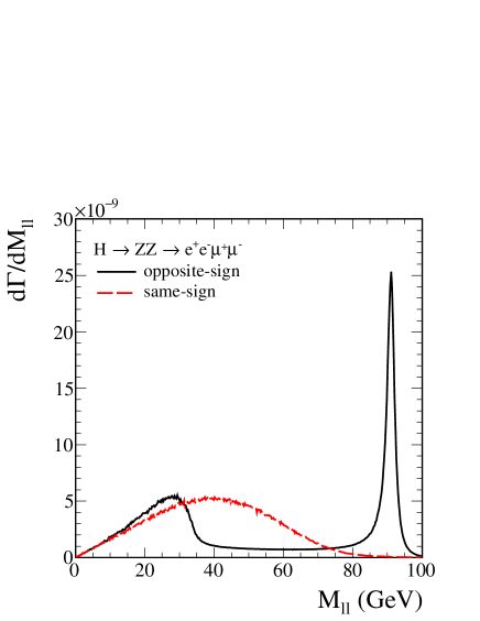
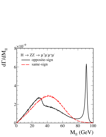
Figure 6: The distributions in $\ell\ell$ invariant mass for the decay $H\to Z^{*}Z^{*}\to e^{+}e^{-}\mu^{+}\mu^{-}$ (left panel) and $H\to Z^{*}Z^{*}\to\mu^{+}\mu^{-}\mu^{+}\mu^{-}$ (right panel).

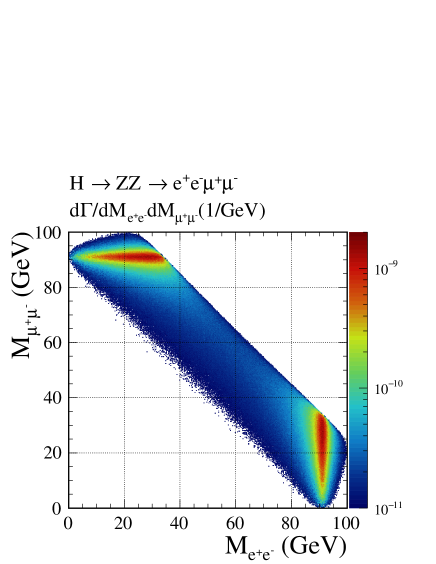
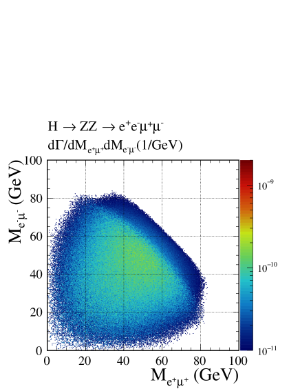
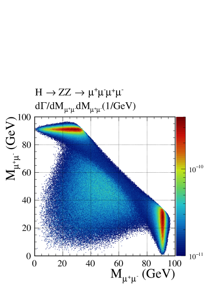
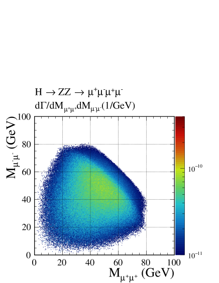
Figure 7: Two-dimensional distributions in dilepton invariant masses for the decay $H\to Z^{*}Z^{*}\to e^{+}e^{-}\mu^{+}\mu^{-}$ (top panels) and $H\to Z^{*}Z^{*}\to\mu^{+}\mu^{-}\mu^{+}\mu^{-}$ (bottom panels).

Interesting observable suitable for the spin-parity assignment is $\phi_{ZZ}$, the angle between the decay planes of the virtual $Z$ bosons in the $H$ rest frame. For the $\phi_{ZZ}$ angle we use the definition Bredenstein:2006rh ; Boselli:2015aha (see also Mikhasenko:2020qor )

$$\cos\phi_{ZZ}=\frac{(\mbox{\boldmath$p_{12}$}\times\mbox{\boldmath$p_{1}$})\cdot(\mbox{\boldmath$p_{2}$}\times\mbox{\boldmath$p_{3}$})}{|\mbox{\boldmath$p_{12}$}\times\mbox{\boldmath$p_{1}$}||\mbox{\boldmath$p_{12}$}\times\mbox{\boldmath$p_{3}$}|}\,,$$

$${\rm sgn}(\sin\phi_{ZZ})={\rm sgn}\{\mbox{\boldmath$p_{12}$}\cdot[(\mbox{\boldmath$p_{12}$}\times\mbox{\boldmath$p_{1}$})\times(\mbox{\boldmath$p_{12}$}\times\mbox{\boldmath$p_{3}$})]\}\,,$$ (53)

where $\mbox{\boldmath$p_{12}$}=\mbox{\boldmath$p_{1}$}+\mbox{\boldmath$p_{2}$}$.

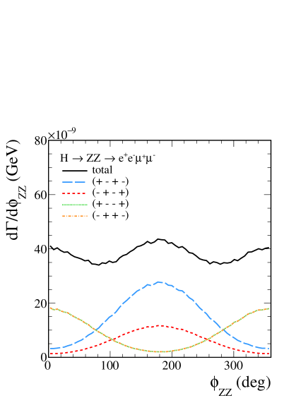
Figure 8: The distribution in $\phi_{ZZ}$ (53) for the decay $H\to Z^{*}Z^{*}\to e^{+}e^{-}\mu^{+}\mu^{-}$. Contributions of different helicities ($2s_{1}$, $2s_{2}$, $2s_{3}$, $2s_{4}$) of the outgoing leptons are shown separately.

In Fig. 8 we present the distribution in $\phi_{ZZ}$ for $H\to Z^{*}Z^{*}\to e^{+}e^{-}\mu^{+}\mu^{-}$. We label the results for different helicity terms as ($2s_{1}$, $2s_{2}$, $2s_{3}$, $2s_{4}$) where $s_{i}=\pm\frac{1}{2}$. The distributions in $\phi_{\ell}$ and $\cos\theta_{\ell}$ are constants for both the decay channels.

We have checked that the helicity amplitudes of $H\to 2e2\mu$ with the helicity spinors (43) and (44) in the massless limit are consistent with those given by Eqs. (9)–(13), (D4), (D5) in Campbell:2013una and by Eq. (A1) in He:2019kgh that uses massless helicity spinor formalism (see also Eqs. (14) and (15) of Dixon:1996wi ).

IV Conclusions

We have presented a new Monte Carlo library Decay and examples of generators that can generate events for the decay of any particle into higher multiplicity final state and provide an easy way of adaptive integration over Lorentz Invariant Phase Space. They integrate with common in High Energy Physics software - ROOT and have a compatible interface with other ROOT generators.

We have also presented a few examples of applications of these tools, namely, decay into two particles, decay into three particles within the $4$-Fermi theory of $\mu$ decay, and the Standard Model Higgs boson decay into four leptons in leading order. Special attention has been devoted to the Higgs boson decay, where we have presented some interesting results which could be studied experimentally. All the tests have turned out to be compatible with results known from the literature.

We hope that in the near future our generator will be a part of the commonly available ROOT software.

- (1) T. Sjöstrand, S. Ask, J. R. Christiansen, R. Corke, N. Desai, P. Ilten, S. Mrenna, S. Prestel, C. O. Rasmussen, and P. Z. Skands, An introduction to PYTHIA 8.2, Comput. Phys. Commun. 191 (2015) 159, arXiv:1410.3012 [hep-ph].
- (2) T. Sjöstrand, S. Mrenna, and P. Z. Skands, PYTHIA 6.4 Physics and Manual, JHEP 05 (2006) 026, arXiv:hep-ph/0603175.
- (3) T. A. Aaltonen et al., (CDF Collaboration), Measurement of central exclusive production in collisions at and 1.96 TeV at CDF, Phys. Rev. D91 (2015) 091101, arXiv:1502.01391 [hep-ex].
- (4) J. Adam et al., (STAR Collaboration), Measurement of the central exclusive production of charged particle pairs in proton-proton collisions at GeV with the STAR detector at RHIC, JHEP 07 (2020) 178, arXiv:2004.11078 [hep-ex].
- (5) A. M. Sirunyan et al., (CMS Collaboration), Study of central exclusive production in proton-proton collisions at = 5.02 and 13 TeV, Eur. Phys. J. C 80 no. 8, (2020) 718, arXiv:2003.02811 [hep-ex].
- (6) R. Sikora, PhD thesis: Measurement of the diffractive central exclusive production in the STAR experiment at RHIC and the ATLAS experiment at LHC, AGH University of Science and Technology, 2020. http://home.agh.edu.pl/~rsikora/files/PhD_RafalSikora.pdf?pdf=PhD_RafalSikora.
- (7) F. James, Monte Carlo phase space. http://cds.cern.ch/record/275743/files/CERN-68-15.pdf.
- (8) ROOT software. http://root.cern.ch/drupal/.
- (9) P. Lebiedowicz, O. Nachtmann, and A. Szczurek, Exclusive diffractive production of via the intermediate and states in proton-proton collisions within tensor Pomeron approach, Phys. Rev. D94 no. 3, (2016) 034017, arXiv:1606.05126 [hep-ph].
- (10) P. Lebiedowicz, O. Nachtmann, and A. Szczurek, Central exclusive diffractive production of via the intermediate state in proton-proton collisions, Phys. Rev. D99 no. 9, (2019) 094034, arXiv:1901.11490 [hep-ph].
- (11) R. A. Kycia, J. Chwastowski, R. Staszewski, and J. Turnau, GenEx: A simple generator structure for exclusive processes in high energy collisions, Commun. Comput. Phys. 24 no. 3, (2018) 860, arXiv:1411.6035 [hep-ph].
- (12) R. A. Kycia, J. Turnau, J. J. Chwastowski, R. Staszewski, and M. Trzebiński, The adaptive Monte Carlo toolbox for phase space integration and generation, Commun. Comput. Phys. 25 no. 5, (2019) 1547, arXiv:1711.06087 [hep-ph].
- (13) R. Kycia, P. Lebiedowicz, A. Szczurek, and J. Turnau, Triple Regge exchange mechanisms of four-pion continuum production in the reaction, Phys. Rev. D95 no. 9, (2017) 094020, arXiv:1702.07572 [hep-ph].
- (14) M. Aaboud et al., (ATLAS Collaboration), Search for heavy resonances in the and final states using proton–proton collisions at TeV with the ATLAS detector, Eur. Phys. J. C 78 no. 4, (2018) 293, arXiv:1712.06386 [hep-ex].
- (15) G. Aad et al., (ATLAS Collaboration), Search for heavy resonances decaying into a pair of bosons in the and final states using 139 fb-1 of proton-proton collisions at TeV with the ATLAS detector, arXiv:2009.14791 [hep-ex].
- (16) GNU GCC. https://gcc.gnu.org/.
- (17) GNU Make. http://www.gnu.org/software/make/.
- (18) Doxygen. https://www.doxygen.nl.
- (19) DECAY library, 2020 (accessed November 30, 2020). https://github.com/rkycia/Decay.
- (20) M. D. Schwartz, Quantum Field Theory and the Standard Model. Cambridge University Press, 3, 2014.
- (21) R. Hagedorn, Relativistic Kinematics: A guide to the kinematic problems of high-energy physics. W.A. Benjamin, New York, Amsterdam, 1964.
- (22) H. Pilkuhn, The interactions of hadrons. North Holland Publishing Company, 1967.
- (23) G. Lepage, A New Algorithm for Adaptive Multidimensional Integration, J. Comput. Phys. 27 (1978) 192.
- (24) T. Ohl, Vegas revisited: Adaptive Monte Carlo integration beyond factorization, Comput. Phys. Commun. 120 (1999) 13, arXiv:hep-ph/9806432.
- (25) G. P. Lepage, Adaptive Multidimensional Integration: VEGAS Enhanced, arXiv:2009.05112 [physics.comp-ph].
- (26) S. Jadach, Foam: A General purpose cellular Monte Carlo event generator, Comput. Phys. Commun. 152 (2003) 55, arXiv:physics/0203033.
- (27) A. Denner, Techniques for the Calculation of Electroweak Radiative Corrections at the One-Loop Level and Results for -Physics at LEP 200, Fortsch. Phys. 41 (1993) 307, arXiv:0709.1075 [hep-ph].
- (28) A. Denner, G. Weiglein, and S. Dittmaier, Application of the background-field method to the electroweak standard model, Nucl. Phys. B 440 (1995) 95, arXiv:hep-ph/9410338.
- (29) M. Kłusek-Gawenda, P. Lebiedowicz, O. Nachtmann, and A. Szczurek, From the reaction to the production of pairs in ultraperipheral ultrarelativistic heavy-ion collisions at the LHC, Phys. Rev. D96 no. 9, (2017) 094029, arXiv:1708.09836 [hep-ph].
- (30) FeynCalc. https://feyncalc.github.io/.
- (31) R. Mertig, M. Bohm, and A. Denner, Feyn Calc - Computer-algebraic calculation of Feynman amplitudes, Comput. Phys. Commun. 64 (1991) 345.
- (32) V. Shtabovenko, R. Mertig, and F. Orellana, FeynCalc 9.3: New features and improvements, Comput. Phys. Commun. 256 (2020) 107478, arXiv:2001.04407 [hep-ph].
- (33) S. Boselli, C. M. Carloni Calame, G. Montagna, O. Nicrosini, and F. Piccinini, Higgs boson decay into four leptons at NLOPS electroweak accuracy, JHEP 06 (2015) 023, arXiv:1503.07394 [hep-ph].
- (34) A. Bredenstein, A. Denner, S. Dittmaier, and M. Weber, Precise predictions for the Higgs-boson decay leptons, Phys. Rev. D 74 (2006) 013004, arXiv:hep-ph/0604011.
- (35) M. Mikhasenko, L. An, and R. McNulty, The determination of the spin and parity of a vector-vector system, arXiv:2007.05501 [hep-ph].
- (36) J. M. Campbell, R. K. Ellis, and C. Williams, Bounding the Higgs width at the LHC using full analytic results for , JHEP 04 (2014) 060, arXiv:1311.3589 [hep-ph].
- (37) H.-R. He, X. Wan, and Y.-K. Wang, Anomalous decay and its interference effects at the LHC, arXiv:1902.04756 [hep-ph].
- (38) L. J. Dixon, Calculating scattering amplitudes efficiently, in Theoretical Advanced Study Institute in Elementary Particle Physics (TASI 95): QCD and Beyond, p. 539. 1, 1996. arXiv:hep-ph/9601359.