Abstract

Neutrinoless double beta ($0\nu\beta\beta$) decay searches are currently among the major foci of experimental physics. The observation of such a decay will have important implications in our understanding of the intrinsic nature of neutrinos and shed light on the limitations of the Standard Model. The rate of this process depends on both the unknown neutrino effective mass and the nuclear matrix element ($M^{0\nu}$) associated with the given $0\nu\beta\beta$  transition. The latter can only be provided by theoretical calculations, hence the need of accurate theoretical predictions of $M^{0\nu}$for the success of the experimental programs. This need drives the theoretical nuclear physics community to provide the most reliable calculations of $M^{0\nu}$. Among the various computational models adopted to solve the many-body nuclear problem, the shell model is widely considered as the basic framework of the microscopic description of the nucleus. Here, we review the most recent and advanced shell-model calculations of $M^{0\nu}$ considering the light-neutrino-exchange channel for nuclei of experimental interest. We report the sensitivity of the theoretical calculations with respect to variations in the model spaces and the shell-model nuclear Hamiltonians.

xx 1 5 Received: date; Accepted: date; Published: date Present Status of Nuclear Shell-Model Calculations of $0\nu\beta\beta$ Decay Matrix Elements Luigi Coraggio ^1,2*, Nunzio Itaco ^1,2, Giovanni De Gregorio ^1,2, Angela Gargano ², Riccardo Mancino ^1,2 and Saori Pastore ³ Luigi Coraggio, Giovanni De Gregorio, Angela Gargano, Nunzio Itaco, Riccardo Mancino and Saori Pastore Correspondence: luigi.coraggio@na.infn.it

1 Introduction

Neutrinoless double beta ($0\nu\beta\beta$) decay is a process in which two neutrons inside the nucleus transform into two protons with the emission of two electrons and no neutrinos. With only two electrons in the final state, lepton number conservation needs to be violated by two units for the process to occur. The observation of $0\nu\beta\beta$ decay would imply that neutrinos are Majorana particles—that is, they are their own antiparticles Schechter and Valle (1982)—and give insight into leptogenesis scenarios for the generation of the observed matter-antimatter asymmetry in the universe Davidson et al. (2008). In fact, $0\nu\beta\beta$ decay is the most promising laboratory probe of lepton number violation and it is, in fact, the subject of intense experimental activities Gando et al. (2013); Agostini et al. (2013); Albert et al. (2014); Andringa et al. (2016); Gando et al. (2016); Elliott et al. (2017); Agostini et al. (2017); Aalseth et al. (2018); Albert et al. (2018); Alduino et al. (2018); Agostini et al. (2018); Azzolini et al. (2018). The current reported $0\nu\beta\beta$ half-lives of ⁷⁶Ge, ¹³⁰Te and ¹³⁶Xe are larger than $8\cdot 10^{25}$ yr Agostini et al. (2018), $1.5\cdot 10^{25}$ yr Azzolini et al. (2018) and $1.1\cdot 10^{26}$ yr Gando et al. (2016), respectively, with next generation ton scale experiments expecting a two orders of magnitude improvement in the half life sensitivity.

Since $0\nu\beta\beta$ decay measurements use atomic nuclei as a laboratory to test the extent of the Standard Model, nuclear theory plays a crucial role in correctly interpreting the experimental data and disentangling nuclear physics effects from unknown lepton number violating mechanisms. The half-life of the $0\nu\beta\beta$ decays is given by

$$\left[T^{0\nu}_{1/2}\right]^{-1}=G^{0\nu}\left|M^{0\nu}\right|^{2}\left|f(m_{i},U_{ei})\right|^{2}~{},$$ (1)

where $G^{0\nu}$ is a phase-space (or kinematic) factor Kotila and Iachello (2012, 2013), $M^{0\nu}$ is the nuclear matrix element (NME), and $f(m_{i},U_{ei})$ is a function of the neutrino masses $m_{i}$ and their mixing matrix elements $U_{ei}$ that accounts for beyond-standard-model physics. Within the light-neutrino exchange mechanisms, $f(m_{i},U_{ei})$ has the following expression:

$$f(m_{i},U_{ei})=g_{A}^{2}\frac{\langle m_{\nu}\rangle}{m_{e}}$$

where $g_{A}$ is the axial coupling constant, $m_{e}$ is the electron mass, and $\langle m_{\nu}\rangle=\sum_{i}(U_{ei})^{2}m_{i}$ is the effective neutrino mass. It is then clear that access to unknown neutrino properties is granted only if $M^{0\nu}$  is calculated with great accuracy.

Currently the calculated matrix elements for nuclei of experimental interest are characterized by large uncertainties. For nuclear systems with medium masses and beyond, the many-body nuclear problem cannot be solved exactly with the available computational resources. For these systems, one is inevitably forced to truncate the model spaces and reduce or neglect the effects of many-body correlations and electroweak currents. As a result, different computational methods provide calculated $M^{0\nu}$swhich differ by a factor of two Engel and Menéndez (2017). On the above grounds, it is clear that reliable calculations of $M^{0\nu}$’s are a prime goal of nuclear many-body investigations.

The ab initio framework for nuclei allows to retain the complexity of many-body correlations and currents. Within this approach nuclei are described as systems made of nucleons interacting via two- and three-body forces. Interactions with external probes, such as electrons, neutrinos, and photons are described using many-body current operators. One- and two-body current operators describe external probes interacting with individual nucleons and pairs of correlated nucleons, respectively. This scheme has been implemented successfully to study light to intermediate mass nuclei within several many-body computational approaches. Due to their prohibitive computational cost, ab initio methods have been used to study $0\nu\beta\beta$  transitions in light nuclei instead. While transitions in light nuclei do not have a direct experimental interest, these studies provide us with an important benchmark to test other many-body methods that can be used to calculate transition matrix elements for heavy-mass nuclei of experimental interest. Further, they allow us to size the importance of the different lepton number violating mechanisms leading to $0\nu\beta\beta$ decay processes, and to quantify the effect of the various approximations used in the many-body methods for medium to large nuclear systems. Studies along this line have been carried out, for example, in Refs. Pastore et al. (2018); Wang et al. (2019); Basili et al. (2020). Only very recently, the ab initio community is venturing calculations of $0\nu\beta\beta$ decay matrix element of experimental relevance, as reported, for example, in Ref. Hergert et al. (2016), where the authors calculate the $M^{0\nu}$  of ⁴⁸Ca—the lightest system where the $Q$-value is compatible with the decay—combining the in-medium similarity renormalization group with the generator-coordinate method Griffin and Wheeler (1957).

Besides the exceptions mentioned above, the nuclear physics community has been primarily focused on employing approximated many-body methods to access heavy open-shell nuclei of experimental interest. These approximated methods generally invoke a truncation of the full Hilbert space of configurations. To account for missing dynamics and degrees of freedom in the nuclear wave functions, the nuclear Hamiltonian is then replaced by an effective or renormalized Hamiltonian, i.e., $H_{\rm eff}$. This procedure is carried out, in general, by fitting parameters inherent the given nuclear model to spectroscopic properties of the nuclei under investigation. Nuclear models adopted to study $0\nu\beta\beta$ decay of nuclei of experimental interest are: the interacting boson model Barea and Iachello (2009); Barea et al. (2012, 2013), the quasiparticle random-phase approximation (QRPA) Sim (2009); Fang et al. (2011); Faessler et al. (2012), the energy density functional methods Rodríguez and Martínez-Pinedo (2010), the covariant density-functional theory Song et al. (2014); Yao et al. (2015); Song et al. (2017); Jiao et al. (2017); Yao et al. (2018); Jiao et al. (2018); Jiao and Johnson (2019), and the shell model (SM) Menéndez et al. (2009a, b); Horoi and Brown (2013); Neacsu and Horoi (2015); Brown et al. (2015). These models agree within a factor of two (see, for example, Fig. 5 of Ref. Engel and Menéndez (2017) and references therein) when calculating $0\nu\beta\beta$ decay matrix elements of $A=48-150$ nuclei. The difference is mostly to be ascribed to the different renormalization procedures adopted by the different models.

In addition to renormalize the nuclear Hamiltonian, in this scheme one has to renormalize the free constants that appear in the definitions of the decay operators—e.g., proton and neutron electric charges, spin and orbital gyromagnetic factors, etc. For example, the axial coupling constant $g_{A}^{free}=1.2723$ Tanabashi and et al (2018) needs to be quenched by a factor of $q$ Towner (1987), because all the aforementioned models usually overestimate Gamow-Teller (GT) rates when compared to the experimental data Chou et al. (1993). The choice of $q$ depends on the nuclear structure model, the dimensions of the reduced Hilbert space, and the mass of the nuclei under investigation Suhonen (2017a). The common procedure to handle the quenching of $g_{A}$ is to fit GT related data (e.g., single-$\beta$ decay strengths, two-neutrino double-$\beta$ decay rates, etc.), and some authors argue that the value of $q$ required to reach agreement between theoretical and experimental values should be also employed to calculate $M^{0\nu}$ (see for instance Refs. Suhonen (2017b, a)). In passing, it is worth mentioning that within the ab initio framework one can utilize the free nucleonic charges, magnetic moments, and axial coupling constant without having to resort to quenching, provided that corrections from two-body currents and two-body correlations are accounted for Park et al. (1993, 1996); Baroni et al. (2016); Krebs et al. (2017, 2020); Pastore et al. (2018); King et al. (2020); Gysbers et al. (2019). In this work, we review the most recent and advanced SM results of $M^{0\nu}$ for nuclei currently candidates for the detection of the $0\nu\beta\beta$ decay in many laboratories around the world. We focus on the sensitivity of the calculations with respect to variations in the model spaces and the shell-model nuclear Hamiltonians, as well as to the variations in the “short-range correlations” which reveal the role of SM correlated wave functions.

The paper is organized as follows: in Section 2 we outline the basics theory of the nuclear SM and short-range correlations, and provide the analytical expressions of the nuclear matrix elements, for both neutrinoless and two-neutrino double beta decay. The latter are reported to assess the validity of the adopted nuclear wave functions. In fact, a comparison with experimental data is clearly possible for two-neutrino double beta decays. Section 3 is devoted to the results of the latest SM calculations for ⁴⁸Ca$\rightarrow^{48}$Ti, ⁷⁶Ge$\rightarrow^{76}$Se, ⁸²Se$\rightarrow^{82}$Kr, ¹³⁰Te$\rightarrow^{130}$Xe, and ¹³⁶Xe$\rightarrow^{136}$Ba $0\nu\beta\beta$ and $2\nu\beta\beta$ decays. Comparisons between experimental and calculated $M^{2\nu}$s are reported at the end of Section 3.2 with a discussion on the $g_{A}$ quenching. Our conclusions are given in Section 4.

2 Theoretical overview

2.1 The nuclear shell model

The nuclear shell model allows for a microscopic description of the structure of the nucleus Mayer (1949); Haxel et al. (1949), and it is the root of most current ab initio approaches (No-Core Shell Model, Coupled Cluster Method, In-Medium Similarity Renormalization Group). It is based on the ansatz that each nucleon inside the nucleus moves independently in a spherically symmetric mean field generated by all other constituents. The mean field is usually described by a Woods-Saxon or a harmonic oscillator (HO) potential supplemented by a strong spin-orbit term.

This basic version of the shell model successfully explains the appearance of protons and/or neutrons “magic numbers”—characterizing nuclei bounded more tightly with respect to their neighbors—along with several nuclear properties Mayer and Jensen (1955), including angular momenta and parity for ground-states of odd-mass nuclei. Within this framework, nucleons arrange themselves in well defined and separated energy levels, i.e., the “shells”. It is worth emphasizing that shell-model wave functions do not include correlations induced by the strong short-range two-nucleon interaction. We will come back to this point later, when we discuss the “short-range correlations” (SRC).

The SM can be further improved, especially its description of low-energy nuclear structure, introducing the “interacting shell model” (ISM) picture. In the ISM, the complex nuclear many-body problem is reduced to a simplified one where only few valence nucleons interact in the reduced model space spanned by a single major shell above an inert core. The valence nucleons interact via a two-body “residual interaction”, that is the part of the interaction which is not already accounted for in the central potential. The inclusion of the residual interaction removes the degeneracy of the states belonging to the same configuration and produces a mixing of different configurations.

The SM Hamiltonian consists of one- and two-body components and associated parameters, namely the single-particle (SP) energies and the two-body matrix elements (TBMEs) of the residual interaction. These parameters account for the degrees of freedom that are not explicitly included in the truncated Hilbert space of configurations. As a matter of fact, SP energies and TBMEs should be determined to include, in an effective way, the excitations of both the core and the valence nucleons into the shells above the model space.

The construction of the effective SM Hamiltonian, $H_{\rm eff}$, can be carried out into two distinct ways. In one approach one starts from realistic two- and three-nucleon forces (see Ref. Machleidt (2017) and references therein for a review on realistic two- and three-nucleon potentials) and derive the effective Hamiltonian from them. The $H_{\rm eff}$  will then have eigenvalues that belong to the set of eigenvalues of the full nuclear Hamiltonian, defined in the whole Hilbert space. The alternative approach is phenomenological. In this case, the SM Hamiltonian one- and two-body components are adjusted to reproduce a selected set of experimental data. For the fitting procedure one could i) use adjustable parameters entering the analytical expressions of the residual interaction, ii) directly consider the Hamiltonian matrix elements as free parameters (see, e.g., Refs. Elliott (1969); Talmi (2003)), or iii) fine tune the TBMEs of a realistic $H_{\rm eff}$  to reproduce the experimental results. The phenomenological approach has been widely utilized since its formulation in the fifties, and it successfully reproduces a huge amount of data and describes some of the most fundamental properties of the structure of atomic nuclei Caurier et al. (2005).

The SM provides suitable and well tested nuclear wave functions for the initial and final states entering the calculation of $M^{0\nu}$ associated with $0\nu\beta\beta$ decays. SM results based on both the realistic and phenomenological $H_{\rm eff}$ are reported in Section 3.

2.2 Short-range correlations

Short-range correlations (SRCs) are required to account for physics that is missing in all models that expand nuclear wave functions in terms of a truncated non-correlated SP basis. In particular, two-body decay operators—such as those entering $0\nu\beta\beta$ decays—acting on an unperturbed (uncorrelated) wave function yield results that are intrinsically different from those obtained acting the real (correlated) nuclear wave function Bethe (1971); Kortelainen et al. (2007). Due to the highly repulsive nature of the short-range two-nucleon interaction, and in order to carry out nuclear structure calculations, one is forced to perform a consistent regularization of the two-nucleon potential, $V^{NN}$, and of any two-body transition operator Wu et al. (1985).

In nuclear structure calculations based on realistic potentials, one has to deal with non-zero values of the non-correlated wave function, $\Phi$, at short distances. This can be appreciated in Fig. 1. However, because of the repulsive nature of the $V^{NN}$ interaction at small inter-particle distances (or equivalently, the repulsive $V^{NN}$ behavior at high-momentum) the correlated wave function, $\Psi$, has to approach zero as the inter-nucleon distance diminishes, and as fast as the core repulsion increases, see Fig. 1.

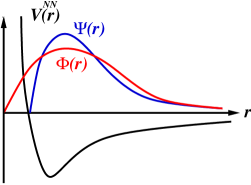
Figure 1: Representation of a realistic potential $V^{NN}$, as a function of the inter-nucleon distance $r$ (black line). The correlated, $\Psi$, and non-correlated, $\Phi$, wave functions are represented by the blue and red lines, respectively. See text for details.

To remedy to this shortcoming, one has to renormalize the short-range (high-momentum) components of the $V^{NN}$ potential whenever a perturbative approach to the many-body problem is pursued. The most common way to soften the matrix elements of the $0\nu\beta\beta$ decay operator is to include SRC given by Jastrow type functions Miller and Spencer (1976); Neacsu et al. (2012). Recently, SRC have been modeled using the Unitary Correlation Operator Method (UCOM) Kortelainen et al. (2007); Menéndez et al. (2009b). This approach prevents the overlap between wave functions of a pair of nucleons Feldmeier et al. (1998).

Another approach has been proposed by some of the present authors in Refs. Coraggio et al. (2019, 2020), where the renormalization of the the $0\nu\beta\beta$ two-body decay operator is carried out consistently with the $V_{{\rm low}\mbox{-}k}$ procedure Bogner et al. (2002) adopted to renormalize the repulsive high-momentum components of the $V^{NN}$ potential. In particular, the renormalization of $V^{NN}$ occurs through a unitary transformation, $\Omega$, which decouples the full momentum space of the two-nucleon Hamiltonian, $H^{NN}$, into two subspaces; the first one is associated with the relative-momentum configurations below a cutoff $\Lambda$ and is specified by a projector operator $P$, the second one is defined in terms of its complement $Q=\mathbf{1}-P$ Coraggio et al. (2019). Being a unitary transformation, $\Omega$ preserves the physics of the original potential for the two-nucleon system, e.g., the calculated values of all nucleon-nucleon observables are the same as those reproduced by solving the Schrödinger equation for two nucleons interacting via $V^{NN}$.

The two-body $0\nu\beta\beta$  operator, $\Theta$, is calculated in the momentum space and renormalized using $\Omega$. This ensure a consistency with the $V^{NN}$ potential, whose high-momentum (short range) components are dumped by the introduction of the cutoff $\Lambda$. The $\Theta$ vertices appearing in the perturbative expansion of the $\hat{\Theta}$ box are substituted with the renormalized $\Theta_{{\rm low}\mbox{-}k}$ operator. The latter is defined as $\Theta_{{\rm low}\mbox{-}k}\equiv P\Omega\Theta\Omega^{-1}P$ for relative momenta $k<\Lambda$, and is set to zero for $k>\Lambda$. The magnitude of the overall effect of this renormalization procedure is comparable to using the SRC modeled by the Unitary Correlation Operator Method Menéndez et al. (2009b), that is a lighter softening of $M^{0\nu}$ with respect to the one provided by Jastrow type SRC Coraggio et al. (2019).

2.3 The $0\nu\beta\beta$-decay operator for the light-neutrino exchange

We now turn our attention to the vertices of the bare $0\nu\beta\beta$ operator, $\Theta$, for the light-neutrino-exchange channel Engel and Menéndez (2017).

We recall that the formal expression of $M_{\alpha}^{0\nu}$—where $\alpha$ stands for Fermi ($F$), Gamow-Teller (GT), or tensor ($T$) decay channels—is written in terms of the one-body transition-density matrix elements between the daughter and parent nuclei (grand-daughter and daughter nuclei) $\langle k|a^{\dagger}_{p^{\prime}}a_{n^{\prime}}|i\rangle$ ($\langle f|a^{\dagger}_{p}a_{n}|k\rangle$). Here, $p$ and $n$ denote proton and neutron states, and $i,k,f$ refer to the parent, daughter, and grand-daughter nuclei, respectively, while $M_{\alpha}^{0\nu}$ reads Sen’kov and Horoi (2013); Šimkovic et al. (2008):

$$M_{\alpha}^{0\nu}= \sum_{k{\cal J}}\sum_{j_{p}j_{p^{\prime}}j_{n}j_{n^{\prime}}}(-1)^{j_{n}+j_{n^{\prime}}+\cal{J}}\hat{\cal{J}}\left\{\begin{array}[]{ccc}j_{p}&j_{n}&J_{\kappa}\\ j_{n^{\prime}}&j_{p^{\prime}}&{\cal J}\end{array}\right\}\left<j_{p}j_{p^{\prime}};{\cal J}\mid\mid\tau^{-}_{1}\tau^{-}_{2}\Theta_{\alpha}^{k}\mid\mid j_{n}j_{n^{\prime}};{\cal J}\right>\langle k||[a^{\dagger}_{p}\otimes\tilde{a}_{n}]_{J_{k}}||i\rangle$$ (4)

$$\langle k||[a^{\dagger}_{n^{\prime}}\otimes\tilde{a}_{p^{\prime}}]_{J_{k}}||f\rangle^{\ast}=\sum_{k}\sum_{j_{p}j_{p^{\prime}}j_{n}j_{n^{\prime}}}\langle f|a^{\dagger}_{p}a_{n}|k\rangle\langle k|a^{\dagger}_{p^{\prime}}a_{n^{\prime}}|i\rangle\times\left<j_{p}j_{p^{\prime}}\mid\tau^{-}_{1}\tau^{-}_{2}\Theta_{\alpha}^{k}\mid j_{n}j_{n^{\prime}}\right>~{},$$ (5)

where the tilde denotes a time-conjugated state, $\tilde{a}_{jm}=(-1)^{j+m}a_{j-m}$.

The operators $\Theta_{\alpha}$ given by Engel and Menéndez (2017):

$$\Theta^{k}_{\rm GT} = \vec{\sigma}_{1}\cdot\vec{\sigma}_{2}H_{\rm GT}^{k}(r)\,,$$ (6)

$$\Theta^{k}_{\rm F} = H_{\rm F}^{k}(r)\,,$$ (7)

$$\Theta^{k}_{\rm T} = \left[3\left(\vec{\sigma}_{1}\cdot\hat{r}\right)\left(\vec{\sigma}_{1}\cdot\hat{r}\right)-\vec{\sigma}_{1}\cdot\vec{\sigma}_{2}\right]H_{\rm T}^{k}(r)~{},$$ (8)

where $H_{\alpha}$ are the neutrino potentials defined as:

$$H_{\alpha}^{k}(r)=\frac{2R}{\pi}\int_{0}^{\infty}\frac{j_{n_{\alpha}}(qr)h_{\alpha}(q^{2})qdq}{q+E_{k}-(E_{i}+E_{f})/2}~{}.$$ (9)

In the equation above, $R=1.2A^{1/3}$ fm, $j_{n_{\alpha}}(qr)$ is the spherical Bessel function, $n_{\alpha}=0$ for Fermi and Gamow-Teller components, while $n_{\alpha}=2$ for the tensor component. For the sake of clarity, the explicit expressions Engel and Menéndez (2017) of neutrino form functions, $h_{\alpha}(q)$, for light-neutrino exchange are reported below:

$$h_{\rm F}({q}^{2}) = g^{2}_{V}({q}^{2})\,,$$

$$h_{\rm GT}({q}^{2}) = \frac{g^{2}_{A}({q}^{2})}{g^{2}_{A}}\left[1-\frac{2}{3}\frac{{q}^{2}}{{q}^{2}+m^{2}_{\pi}}+\frac{1}{3}(\frac{{q}^{2}}{{q}^{2}+m^{2}_{\pi}})^{2}\right]$$

$$+\frac{2}{3}\frac{g^{2}_{M}({q}^{2})}{g^{2}_{A}}\frac{{q}^{2}}{4m^{2}_{p}},$$

$$h_{\rm T}({q}^{2}) = \frac{g^{2}_{A}({q}^{2})}{g^{2}_{A}}\left[\frac{2}{3}\frac{{q}^{2}}{{q}^{2}+m^{2}_{\pi}}-\frac{1}{3}(\frac{{q}^{2}}{{q}^{2}+m^{2}_{\pi}})^{2}\right]$$ (10)

$$+\frac{1}{3}\frac{g^{2}_{M}({q}^{2})}{g^{2}_{A}}\frac{{q}^{2}}{4m^{2}_{p}}\,,$$

For the vector, $g_{V}({q}^{2})$, axial-vector, $g_{A}({q}^{2})$, and weak-magnetism, $g_{M}({q}^{2})$, form factors we use the dipole approximation:

$$g_{V}({q}^{2}) = \frac{g_{V}}{(1+{q}^{2}/{\Lambda^{2}_{V}})^{2}},$$

$$g_{M}({q}^{2}) = (\mu_{p}-\mu_{n})g_{V}({q}^{2}),$$

$$g_{A}({q}^{2}) = \frac{g_{A}}{(1+{q}^{2}/{\Lambda^{2}_{A}})^{2}},$$ (11)

where $g_{V}=1$, $g_{A}\equiv g_{A}^{free}=1.2723$, $(\mu_{p}-\mu_{n})=4.7$, and the cutoff parameters $\Lambda_{V}=850$ MeV and $\Lambda_{A}=1086$ MeV.

The total nuclear matrix element $M^{0\nu}$ can be then written as

$$M^{0\nu}=M_{\rm GT}^{0\nu}-\frac{g_{V}^{2}}{g_{A}^{2}}M_{\rm F}^{0\nu}+M_{\rm T}^{0\nu}~{}~{}.$$ (12)

The expression in Eq. (5) can be easily calculated within the QRPA computational approach, while all other models—including most of the SMs—have to resort to the closure approximation. This approximation is based on the observation that the relative momentum $q$ of the neutrino, appearing in the propagator of Eq. (9), is of the order of 100-200 MeV Engel and Menéndez (2017), while the excitation energies of the nuclei involved in the transition are of the order of 10 MeV Sen’kov and Horoi (2013). It is then customary to replace the energies of the intermediate states, $E_{k}$, appearing in Eq. (9), by an average value $E_{k}-(E_{i}+E_{f})/2\rightarrow\langle E\rangle$. This allow us to simplify both Eqs. (5) and (9). In particular, $M_{\alpha}^{0\nu}$ can be re-written in terms of the two-body transition-density matrix elements $\langle f|a^{\dagger}_{p}a_{n}a^{\dagger}_{p^{\prime}}a_{n^{\prime}}|i\rangle$ as

$$M_{\alpha}^{0\nu} = \sum_{j_{n}j_{n^{\prime}}j_{p}j_{p^{\prime}}}\langle f|a^{\dagger}_{p}a_{n}a^{\dagger}_{p^{\prime}}a_{n^{\prime}}|i\rangle$$

$$\times\left<j_{p}j_{p^{\prime}}\mid\tau^{-}_{1}\tau^{-}_{2}\Theta_{\alpha}\mid j_{n}j_{n^{\prime}}\right>~{},$$ (13)

and the neutrino potentials become

$$H_{\alpha}(r)=\frac{2R}{\pi}\int_{0}^{\infty}\frac{j_{n_{\alpha}}(qr)h_{\alpha}(q^{2})qdq}{q+\left<E\right>}~{}.$$ (14)

Most SM calculations adopt the closure approximation to define the $\Theta$ operators given in Eqs. (6)–(8), and take the average energies $\left<E\right>$ from the evaluations of Refs. Haxton and Stephenson Jr. (1984); Tomoda (1991). It is important to point out that the authors of Ref. Sen’kov and Horoi (2013) performed SM calculations of $M^{0\nu}$ for ⁴⁸Ca both within and beyond the closure approximation, and found that in the second case the results are $\sim 10\%$ larger.

In most cases, short-range correlations are included when computing the radial matrix elements of the neutrino potentials $\left<\psi_{nl}(r)|H_{\alpha}|\psi_{n^{\prime}l^{\prime}}(r)\right>$. In particular, the HO wave functions $\psi_{nl}(r)$ and $\psi_{n^{\prime}l^{\prime}}(r)$ are corrected by a factor $[1+f(r)]$, which takes into account the short range correlations induced by the nuclear interaction

$$\psi_{nl}(r)\rightarrow\left[1+f(r)\right]\psi_{nl}(r)\ .$$ (15)

The functional form of the correlation function $f(r)$ is usually written using a Jastrow-like parametrization as Neacsu et al. (2012)

$$f(r)=-c\cdot e^{-ar^{2}}\left(1-br^{2}\right)~{}~{},$$ (16)

where $a$, $b$ and $c$ are parameters whose values depend on the renormalization procedure adopted to renormalize the non-correlated HO wave functions, (e.g., Jastrow or UCOM schemes, see Section 2.2 for details). In Table 1 we report the values of the $a$, $b$ and $c$ constants commonly employed in SM calculations. In addition to the values proposed by Miller and Spencer Miller and Spencer (1976), we show those based on the modern nucleon-nucleon interactions CD-Bonn and AV18 and derived in Ref. Sim (2009).

Table 1: Values of the SRC parameters.

	a	b	c
Miller-Spencer	1.10	0.68	1.00
CD-Bonn	1.52	1.88	0.46
AV18	1.59	1.45	0.92

2.4 The $2\nu\beta\beta$-decay operator

As already pointed out in the Introduction, because of the impossibility to compare the theoretical values of $M^{0\nu}$  with the experiment, one has to find another way to check the reliability of the computed results. A viable route that is often considered in literature is the calculation of the standard or ordinary two-neutrinos double beta decay transitions where one observes the emission of two electrons and two antineutrinos. Two-neutrino double beta decays are simply the occurrence of two single beta decay transitions inside a nucleus. They differ from $0\nu\beta\beta$  decays in the characteristic value of momentum transfer, which is negligible in ordinary decays and of the order of hundreds of MeVs in $0\nu\beta\beta$  decay. Here, we list the expressions of the GT and Fermi components of the two-neutrinos double beta decay matrix elements $M^{2\nu}$, namely

$$M_{\rm GT}^{2\nu} = \sum_{n}\frac{\langle 0^{+}_{f}||\vec{\sigma}\tau^{-}||1^{+}_{n}\rangle\langle 1^{+}_{n}||\vec{\sigma}\tau^{-}||0^{+}_{i}\rangle}{E_{n}+E_{0}}~{}~{},$$ (17)

$$M_{\rm F}^{2\nu} = \sum_{n}\frac{\langle 0^{+}_{f}||\tau^{-}||0^{+}_{n}\rangle\langle 0^{+}_{n}||\tau^{-}||0^{+}_{i}\rangle}{E_{n}+E_{0}}~{}~{}.$$ (18)

In the equation above, $E_{n}$ is the excitation energy of the $J^{\pi}=0^{+}_{n},1^{+}_{n}$ intermediate state, and $E_{0}=\frac{1}{2}Q_{\beta\beta}(0^{+})+\Delta M$, where $Q_{\beta\beta}(0^{+})$ and $\Delta M$ are the $Q$ value of the transition and the mass difference of the initial and final nuclear states, respectively. The index $n$ runs over all possible intermediate states induced by the given transition operator.

It should be pointed out that the Fermi component is zero in Hamiltonians that conserve the isospin, and most of the SM effective Hamiltonians do. It would play a marginal role only when isospin violation mechanisms are introduced, for example, to account for the effects of the Coulomb force acting between the valence protons Haxton and Stephenson Jr. (1984); Elliott and Petr (2002). In practice, in most calculations, the Fermi component is neglected altogether.

An efficient way to calculate $M^{2\nu}$ is to resort to the Lanczos strength-function method Caurier et al. (2005), which allows to include the intermediate states required to obtain a given accuracy for the calculated values.

The theoretical values are then compared with the experimental counterparts, that are extracted from the observed half life $T^{2\nu}_{1/2}$

$$\left[T^{2\nu}_{1/2}\right]^{-1}=G^{2\nu}\left|M_{\rm GT}^{2\nu}\right|^{2}~{}~{}.$$ (19)

One can base the evaluation of the $M_{\rm GT}^{2\nu}$ on the closure approximation, commonly adopted to study $0\nu\beta\beta$-decay NMEs Haxton and Stephenson Jr. (1984). Within this approximation, one can avoid to explicitly calculate the intermediate $J^{\pi}=1^{+}_{n}$ states. The drawback is that, in using the closure on the intermediate states, the two one-body transition operators become a two-body operator.

This approximation is more adapt to evaluate $M^{0\nu}$where the neutrino’s momentum is about one order of magnitude greater than the average excitation energy of the intermediate states. This allows to safely neglect intermediate-state-dependent energies from the energy denominator appearing in the neutrino potential (see discussion in Section 2.3). Conversely, the closure approximation has turned out to be unsatisfactory when used to calculate $M^{2\nu}$, and that is because the momentum transfer in $2\nu\beta\beta$ process are much smaller. Theoretical calculations of $M^{2\nu}$are discussed in the next session.

3 Shell-model results

In this Section, we report SM results for $M^{0\nu}$  based on both the phenomenological and realistic $H_{\rm eff}$’s. All the calculations are based on the light-neutrino-exchange hypothesis, and the values of all the input parameters are the same as reported in Section 2.3. The only exception is the $g_{A}$ parameter, whose adopted value is equal to 1.254 in some reported calculations. It is worth pointing out, however, that in Ref. Neacsu and Stoica (2013), where it can be found a detailed analysis of the sensitivity of the $M^{0\nu}$results on the values of the input parameters, it has been shown that the effects of such a tiny difference in $g_{A}$ are negligible. We will focus our attention on the ⁴⁸Ca, ⁷⁶Ge, ⁸²Se, ¹²⁸Te, ¹³⁰Te and ¹³⁶Xe emitters. These results have been obtained performing a complete diagonalizations of $H_{\rm eff}$. The latter has been defined in different valence spaces tailored for the specific decay under investigation. All the calculations based on phenomenological interactions are performed starting from Brueckner $G$-matrix elements “fine tuned” to reproduce some specific set of spectroscopic data.

3.1 Results from phenomenological $H_{\rm eff}$’s

We test different phenomenological $H_{\rm eff}$’s. All these interactions have been derived modifying the matrix elements of a $G$-matrix so as to reproduce a chosen set of spectroscopic properties of some nuclei belonging to the mass region of interest. With this procedure one can end up with results that provide similar descriptions of the nuclei under consideration, nevertheless the phenomenological TBMEs are quite different each other.

It is worth stressing out that the calculated $M^{0\nu}$s , reported in this section, are obtained using free value of the axial coupling constant $g_{A}$ without any quenching factor.

The double-magic nucleus ⁴⁸Ca is the lightest emitter investigated in regular $\beta\beta$ decay searches. The SM calculation for $M^{0\nu}$ is obtained using the model space spanned by four neutron and proton single-particle orbitals 0f_7/2, 1p_3/2, 1p_1/2, and 0f_5/2. It is worth mentioning that the regular $\beta\beta$ decay of ⁴⁸Ca is a paradigm for shell-model calculations. Because within the $pf$ model space all spin-orbit partners are present, the Ikeda sum rule is satisfied Ikeda (1964).

Several phenomenological SM effective interactions have been developed to describe $pf$-shell nuclei. Among these are the GXPF1 Honma et al. (2004), GXPF1A Honma et al. (2005), KB3 Poves and Zuker (1981), KB3G Poves et al. (2001), and FPD6 Richter et al. (1991) interactions. In Table 2, we compare the most recent results for the $M^{0\nu}$  of ⁴⁸Ca obtained using the GXPF1A Sen’kov and Horoi (2013) and KB3G interactions Menendez (2018).

Table 2: $M^{0\nu}$ of ⁴⁸Ca. (a) and (b) denote AV18 and CD-Bonn SRC parametrizations, respectively. The results have been taken from Refs. Sen’kov and Horoi (2013); Menendez (2018)

	GXPF1A (a)	KB3G (a)	KB3G (b)
$M_{\rm GT}^{0\nu}$	0.68	0.85	0.93
$M_{\rm F}^{0\nu}$	-0.20	-0.23	-0.25
$M_{\rm T}^{0\nu}$	-0.08	-0.06	-0.06
$M^{0\nu}$	0.73	0.93	1.02

For the medium-mass emitters ⁷⁶Ge and ⁸²Se, the calculations adopt the valence space with the four neutron and proton single-particle orbitals 0f_5/2, 1p_3/2, 1p_1/2, 0g_9/2 outside doubly-magic ⁵⁶Ni, as for instance in Refs. Sen’kov et al. (2014) and Menendez (2018), where the effective interactions GCN2850 Menéndez et al. (2009b) and JUN45 Honma et al. (2009) have been employed. These results are given in Tables 3 and 4.

Table 3: Same as Table 2, but for ⁷⁶Ge. Results are from Refs. Sen’kov et al. (2014); Menendez (2018).

	JUN45 (a)	JUN45 (b)	GCN2850 (a)	GCN2850 (b)
$M_{\rm GT}^{0\nu}$	2.98	3.15	2.56	2.73
$M_{\rm F}^{0\nu}$	-0.62	-0.67	-0.54	-0.59
$M_{\rm T}^{0\nu}$	-0.01	-0.01	-0.01	-0.01
$M^{0\nu}$	3.15	3.35	2.89	3.07

Table 4: Same as Table 2, but for ⁸²Se. Results are from Refs. Sen’kov et al. (2014); Menendez (2018).

	JUN45 (b)	GCN2850 (a)	GCN2850 (b)
$M_{\rm GT}^{0\nu}$	2.75	2.41	2.56
$M_{\rm F}^{0\nu}$	-0.61	-0.51	-0.55
$M_{\rm T}^{0\nu}$	-0.01	-0.01	-0.01
$M^{0\nu}$	3.13	2.73	2.90

Finally, in Tables 5 and 6 we report and compare the calculated $M^{0\nu}$  for ¹³⁰Te and ¹³⁶Xe. These are based on two different effective interactions, namely the SVD Qi and Xu (2012) and the GCN5082 Menéndez et al. (2009b) defined in the $jj55$ valence space spanned by the neutron and proton orbitals 0g_7/2, 1d_5/2, 1d_3/2, 2s_1/2, and 0h_11/2. Results with the SVD and GCN5082 interactions are taken, respectively, from Refs. Neacsu and Horoi (2015) and Menendez (2018).

Table 5: Same as Table 2, but for ¹³⁰Te. Results are from Refs. Neacsu and Horoi (2015); Menendez (2018).

	SVD (a)	SVD (b)	GCN5082 (a)	GCN5082 (b)
$M_{\rm GT}^{0\nu}$	1.54	1.66	2.36	2.54
$M_{\rm F}^{0\nu}$	-0.40	-0.44	-0.62	-0.67
$M_{\rm T}^{0\nu}$	-0.01	-0.01	0.00	0.00
$M^{0\nu}$	1.80	1.94	2.76	2.96

Table 6: Same as Table 2, but for ¹³⁶Xe. Results are from Refs. Neacsu and Horoi (2015); Menendez (2018).

	SVD (a)	SVD (b)	GCN5082 (a)	GCN5082 (b)
$M_{\rm GT}^{0\nu}$	1.39	1.50	2.56	2.73
$M_{\rm F}^{0\nu}$	-0.37	-0.40	-0.50	-0.54
$M_{\rm T}^{0\nu}$	-0.01	-0.01	0.00	0.00
$M^{0\nu}$	1.63	1.76	2.28	2.45

From the results shown above, it can be inferred that the effect associated with using different SRCs does not exceed 10%, while different effective interactions can provide results differing up to 50%. The results reported in this Section are based on the closure approximation. As discussed above, Senkov and coworkers have shown in a series of papers Sen’kov and Horoi (2013); Sen’kov et al. (2014); Sen’kov and Horoi (2016) that in going beyond this approximation, the $0\nu\beta\beta$ decay $M^{0\nu}$becomes about $10\%$ larger.

We recall that the results reported in Tables 2-6 are obtained without quenching the axial coupling constant. However, the calculations based on the empirical SM Hamiltonians so far considered need a quenching factor $q$ different from 1 to reproduce the experimental values of the nuclear matrix elements of the corresponding $2\nu\beta\beta$-decays $M^{2\nu}$s. This can be appreciated in Table 7 where we list the $M^{2\nu}$s calculated with the empirical effective Hamiltonians GXPF1A, KB3G, JUN45, GCN2850 and GCN5082, and compare them with the experimental data. In these calculations, that are performed employing the Lanczos strength-function method Caurier et al. (2005), it has been used the unquenched value of $g_{A}$ (or equivalently a quenching factor $q=1$), and, as expected, the theory is systematically overpredicting the experimental data.

Table 7: $M^{2\nu}$s for ⁴⁸Ca, ⁷⁶ Ge, ⁸²Se, ¹³⁰Te, and ¹³⁶Xe $2\nu\beta\beta$-decay calculated with GXPF1A, KB3G, JUN45, GCN2850, and GCN5082 interactions and compared with data Alexander (2020), there are no published results based on the SVD interaction. These calculations use a quenching factor $q=1$. The values of $M^{2\nu}$s  are reported in MeV^-1.

48Ca$\rightarrow^{48}$Ti	GXPF1A	KB3G	Expt.
	0.0511 Kostensalo and Suhonen (2020)	0.088 Caurier et al. (2012)	$0.035\pm 0.003$
76Ge$\rightarrow^{76}$Se	JUN45	GCN2850	Expt.
	0.333 Caurier et al. (2012)	0.322 Caurier et al. (2012)	$0.106\pm 0.004$
82Se$\rightarrow^{82}$Kr	JUN45	GCN2850	Expt.
	0.344 Caurier et al. (2012)	0.350 Caurier et al. (2012)	$0.085\pm 0.001$
130Te$\rightarrow^{130}$Xe	GCN5082		Expt.
	0.132 Caurier et al. (2012)		$0.0293\pm 0.0009$
136Xe$\rightarrow^{136}$Ba	GCN5082		Expt.
	0.123 Caurier et al. (2012)		$0.0181\pm 0.0006$

3.2 Results from realistic $H_{\rm eff}$’s

In the realistic SM (RSM), $H_{\rm eff}$  is constructed from realistic $V^{NN}$ potentials. This is achieved via a similarity transformation utilized to constrain both the SM Hamiltonian and the SM transition operators. More details on this procedure can be found in the papers by B. H. Brandow Brandow (1967), T. T. S. Kuo and coworkers Kuo et al. (1971); Krenciglowa and Kuo (1974), and K. Suzuki and S. Y. Lee Lee and Suzuki (1980); Suzuki and Lee (1980). Perturbative and non-perturbative derivations of $H_{\rm eff}$  have been most recently reviewed in Ref. Coraggio et al. (2012) and Ref. Stroberg et al. (2019), respectively. The derivation of effective SM decay operators carried out consistently with $H_{\rm eff}$ is discussed in Refs. Ellis and Osnes (1977); Suzuki and Okamoto (1995). Fundamental contributions to the field have been made by I. S. Towner, who has extensively investigated the role of many-body correlations induced by the truncation of the Hilbert space, especially for spin- and spin-isospin-dependent one-body decay operators Towner and Khanna (1983); Towner (1987).

The first calculations of $M^{0\nu}$  starting from realistic $V^{NN}$ potentials and associated effective SM decay operators, were made by Kuo and coworkers in the middle of 1980’s for ⁴⁸Ca Wu et al. (1985). In that reference, $H_{\rm eff}$  and the associated transition operators were based on the Paris and the Reid potentials Lacombe et al. (1980); Reid (1968). The short-range repulsive behavior was renormalized by calculating the corresponding Brueckner reaction matrices Krenciglowa et al. (1976). Many-body perturbation theory was then implemented to derive both the TBMEs of $H_{\rm eff}$  and the effective $0\nu\beta\beta$-decay operator. The effect of the SRC was embedded in the defect wave function Kuo and Brown (1966), consistently with the renormalization procedure from the Paris and Reid potentials. Finally, the authors calculated the half lives of ⁴⁸Ca $0\nu\beta\beta$-decay, for both light- and heavy-neutrino exchange, as a function of the neutrino effective mass.

In more recently, J. D. Holt and J. Engel calculated effective SM operators $\Theta_{\rm eff}$’s from modern chiral effective field theory $V^{NN}$ potentials. In particular, they started from the chiral $V^{NN}$ potential by Entem and Machleidt Entem and Machleidt (2002) and cured its perturbative behavior using the $V_{{\rm low}\mbox{-}k}$ procedure Bogner et al. (2002). The $\Theta_{\rm eff}$ was expanded up to third order in perturbation theory and used to calculate $M^{0\nu}$ for ⁷⁶Ge, ⁸²SeHolt and Engel (2013), and ⁴⁸CaKwiatkowski et al. (2014). The effects of SRC was included via an effective Jastrow function obtained from Brueckner-theory calculations Sim (2009). For ⁷⁶Ge and ⁸²Se decays, the authors employed the empirical GCN2850 Menéndez et al. (2009b) and JUN45 Honma et al. (2009) SM interactions, respectively, and for the $0\nu\beta\beta$ decay of ⁴⁸Ca they used the GXPF1A $H_{\rm eff}$ Honma et al. (2005). The values obtained by Holt and Engel in the light-neutrino exchange channel are $M^{0\nu}$=1.30 for ⁴⁸Ca , $M^{0\nu}$=3.77 for ⁷⁶Ge, and $M^{0\nu}$=3.62 for ⁸²Se Holt and Engel (2013); Kwiatkowski et al. (2014).

In Ref. Holt and Engel (2013), the authors calculated also the ⁷⁶Ge $2\nu\beta\beta$  matrix element. The calculation used the closure approximation. However, as we discussed in Sessions 2.3 and 2.4, this approximation is not robust when applied to study $2\nu\beta\beta$ processes where the values of momentum transfer are small. In fact, the authors obtain a result for ⁷⁶Ge $M_{\rm GT}^{2\nu}$ that is about two times larger than the one calculated with the Lanczos strength-function method Horoi (2013); Brown et al. (2015), and about 5 times larger than the experimental value Alexander (2020).

RSM calculations based on the high-precision CD-Bonn $NN$ potential Machleidt (2001) have been recently carried out in Ref. Coraggio et al. (2020), where the repulsive high-momentum components have been integrated out through the $V_{{\rm low}\mbox{-}k}$ technique with “hard cutoff” $\Lambda=2.6$ fm^-1 Bogner et al. (2002). The $M^{0\nu}$’s have been calculated within the SM using $H_{\rm eff}$, and effective decay operators $\Theta_{\rm eff}$’s up to the third order in perturbation theory. Two-body matrix elements entering the $0\nu\beta\beta$-decay operator have been renormalized consistently within the $V_{{\rm low}\mbox{-}k}$ to account for short-range correlations (see Section 2.2 for more details), and Pauli-principle violations in the effective SM operator. It should be pointed out that calculations of systems with a number $n$ of valence nucleons require the derivation of $n$-body effective operators, that take into account the evolution of the number of valence particle in the model space $P$. The correlation between $P$-space configurations and those belonging to $Q$ space is affected by the filling of the model-space orbitals, and in a perturbative expansion of SM operators this is considered by way of $n$-body diagrams. This is called the “Pauli-blocking effect” and calculations in Ref. Coraggio et al. (2020), where all SM parameters have been consistently derived from the realistic $V^{NN}$ potential without any empirical adjustments, take it into consideration by including the contribution of three-body correlation diagrams to derive $\Theta_{\rm eff}$.

The results for $0\nu\beta\beta$ decay in the light-neutrino exchange channel of ⁴⁸Ca, ⁷⁶Ge, ⁸²Se, ¹³⁰Te, and ¹³⁶Xe are reported in Table 8.

Table 8: $M^{0\nu}$s of ⁴⁸Ca, ⁷⁶Ge, ⁸²Se, ¹³⁰Te, and ¹³⁶Xe decays obtained with the realistic effective Hamiltonians and operators Coraggio et al. (2020). The tensor component has been neglected.

Decay	$M^{0\nu}_{\rm GT}$	$M^{0\nu}_{\rm F}$	$M^{0\nu}$
48Ca $\rightarrow$ 48Ti	0.22	-0.12	0.30
76Ge $\rightarrow$ 76Se	2.25	-0.65	2.66
82Se $\rightarrow$ 82Kr	2.31	-0.66	2.72
130Te $\rightarrow$ 130Xe	2.66	-0.80	3.16
136Xe $\rightarrow$ 136Ba	2.01	-0.61	2.39

It is worth pointing out that this approach to SM calculations has been successfully tested on energy spectra, electromagnetic transition strengths, GT strength distributions, and nuclear matrix elements for the two-neutrino $\beta\beta$ decay Coraggio et al. (2017, 2019), without resorting to effective proton/neutron charges and gyromagnetic factors, or quenching of $g_{A}$. In Table 9 we report the the calculated values of $M^{2\nu}$  from Ref. Coraggio et al. (2019) and compare them with experimental data Alexander (2020).

Table 9: Same as in Table 7, but the calculated values Coraggio et al. (2019) are obtained employing effective Hamiltonians and decay operators derived starting from the CD-Bonn realistic potential (see text for details) and compared with experiment Alexander (2020).

48Ca$\rightarrow^{48}$Ti	Theory	Expt.
	0.026	$0.035\pm 0.003$
76Ge$\rightarrow^{76}$Se	Theory	Expt.
	0.104	$0.106\pm 0.004$
82Se$\rightarrow^{82}$Kr	Theory	Expt.
	0.109	$0.085\pm 0.001$
130Te$\rightarrow^{130}$Xe	Theory	Expt.
	0.061	$0.0293\pm 0.0009$
136Xe$\rightarrow^{136}$Ba	Theory	Expt.
	0.0341	$0.0181\pm 0.0006$

A few comments are now in order. As we already pointed out in the Introduction, SM calculations overestimate $M^{2\nu}$ and Gamow-Teller transition strengths. To remedy to this deficiency one introduces a quenching factor $q$ that is multiplied to $g_{A}$ to reduce the values of the calculated matrix elements. This factor depends on i) the mass region of the nuclei involved in the decay process; and ii) the dimension of the model space used in the calculation. The quenching factor has on average the empirical value $q\approx 0.7$ Suhonen (2017a)).

The quenching factor accounts for missing correlations and missing many-body effects in the transition operators. The truncation of the full Hilbert space to the reduced SM space has the effect of excluding all correlations between the model-space configurations and the configurations belonging to either the doubly-closed core or the shells placed in energies above the SM space. In addition, SM calculations are based on the single-nucleon paradigm for the transition operators. However, two-body electroweak currents Park et al. (1993, 1996); Baroni et al. (2016); Krebs et al. (2017, 2020); Pastore et al. (2018); King et al. (2020); Gysbers et al. (2019); Pastore et al. (2008, 2009, 2011, 2014, 2013); Piarulli et al. (2013); Kolling et al. (2009, 2011); Bacca and Pastore (2014) are found to play a role in several electroweak observables. These involve the exchange of mesons and nucleonic excitations.

I. S. Towner extensively studied how to construct effective $\beta$-decay operators that account for the degrees of freedom that are not explicitly included in the model space (see Ref. Towner (1987)). This has been more recently investigated in Refs. Coraggio et al. (2017, 2019)). The results that are reported in Table 9 demonstrate a satisfactory agreement with the data can be obtained without resorting to quenching factors $q$ if one employs effective GT operators within the SM.

Moreover, in Ref. Coraggio et al. (2020) the authors showed that, the renormalization procedure implemented to account for missing configurations plays a marginal role in the calculated $M^{0\nu}$s, while it is relevant in $2\nu\beta\beta$-decay induced by the one-body GT operator. This evidences that the mechanisms which underlies the renormalization of the one-body single-$\beta$ and the two-body $0\nu\beta\beta$ decay operators are different.

In closing, we address the role of many-body electroweak currents in the redefinition of single-$\beta$-decay and $0\nu\beta\beta$-decay operators. Within the shell model, one can use nuclear potentials derived within chiral perturbation theory Fukui et al. (2018); Ma et al. (2019), and include also the contributions of chiral two-body electroweak currents. Studies along these lines have been recently carried out in Refs.Gysbers et al. (2019); Menéndez et al. (2011); Wang et al. (2018), where the authors find significant contributions from two-body axial currents in $\beta$-decay. Concurrently, a study reported in Ref. Rho (2019) argues that many-body electroweak currents should play a negligible role in standard GT transitions (namely, $\beta$- and $2\nu\beta\beta$ decays) due to the “chiral filter” mechanismRho (2019). The chiral filter mechanism may be no longer valid for $0\nu\beta\beta$ decay since the transferred momentum is $\sim 100$ MeV, which will require further investigations to fully understand the role of many-body currents in SM calculations of $M^{0\nu}$s.

3.3 Comparison between SM calculations

In Fig. 2, we group most of the SM results for ⁴⁸Ca$\rightarrow$ ⁴⁸Ti, ⁷⁶Ge $\rightarrow$ ⁷⁶Se, ⁸²Se $\rightarrow$ ⁸²Kr, ¹³⁰Te $\rightarrow$ ¹³⁰Xe, and ¹³⁶Xe $\rightarrow$ ¹³⁶Ba. We have chosen the results according to the following criteria:

1. All the SM calculations for a given transition are based on the same model space.

2. All the calculations use the closure approximation.

3. Whenever the calculations use different choices of SRCs, the average value and associated error bar is reported.

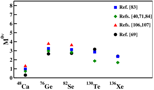
Figure 2: $M^{0\nu}$’s calculated using different $H_{\rm eff}$ and $0\nu\beta\beta$-decay operators. Blue squares represent the results based on the Strasbourg-Madrid $H_{\rm eff}$’s Menendez (2018). Green diamonds correspond to the calculations by Horoi and coworkers Neacsu and Horoi (2015); Sen’kov and Horoi (2013); Sen’kov et al. (2014). Results by Holt and Engel are indicated by the red triangles Holt and Engel (2013); Kwiatkowski et al. (2014). Black dots indicate results by some of the present authors reported in Ref. Coraggio et al. (2020).

The scale on the y-axis is consistent with the one employed in Fig. 5 of Ref. Engel and Menéndez (2017). We stress that our criteria rule out, for the sake of consistency, results from SM calculations where alternative approaches have been followed. For example, we recall that Horoi and coworkers have extensively performed calculations beyond the closure approximation Sen’kov and Horoi (2013); Sen’kov et al. (2014); Sen’kov and Horoi (2016). In particular, as already mentioned several times, results for the $M^{0\nu}$  of ⁴⁸Ca calculated with and without the closure approximation differ by $\sim 10\%$. Likewise, we neglect the results of large-scale SM calculations, where model spaces larger than a single major shell are used. This is the case, for instance, of the work by Horoi and Brown Horoi and Brown (2013) and by Iwata and coworkers Iwata et al. (2016). In the former, it was shown how the enlargement of the standard $g_{9/2}dsh_{9/2}$ model space by the inclusion of the spin-orbit partners of g_9/2 and h_9/2 orbitals leads to a 10-30% reduction of the calculated $M^{0\nu}$for the ¹³⁶Xe emitter. In the latter, the authors reported the results for the $M^{0\nu}$of ⁴⁸Ca based on large-scale shell-model calculations including two harmonic oscillator shells ($sd$ and $pf$ shells). They found that $M^{0\nu}$is enhanced by about 30% with respect to $pf$-shell calculations when excitations up to $2\hbar\omega$ are explicitly included.

The spread among different results is rather narrow, except from the ¹³⁰Te $\rightarrow$ ¹³⁰Xe $0\nu\beta\beta$ decay since the result in Ref. Neacsu and Horoi (2015) are more than $30\%$ larger than those in Refs. Menendez (2018); Coraggio et al. (2020). We observe that the results from Refs. Menendez (2018); Coraggio et al. (2020) are close each other, and the $M^{0\nu}$’s calculated by Holt and Engel Holt and Engel (2013); Kwiatkowski et al. (2014) are consistently larger than those from other SM calculations. The computational methods reported in the figure use substantially different SM effective Hamiltonians, yet they all lead to equally satisfactory results for a large amount of structure data. This leads us to argue that the SM approach is reliable for the study of $0\nu\beta\beta$ decay.

Finally, comparing Fig. 2 with the compilation of results reported in Fig. 5 in Ref. Engel and Menéndez (2017), we confirm that also these more recent SM calculations provide values that are smaller than those obtained with other nuclear models such as the Interacting Boson Model, the QRPA, and Energy Density Functional methods. Since the advantage of the nuclear shell model with respect to other approaches is to include a larger number of nuclear correlations, one may argue that by enlarging the dimension of the Hilbert space of nuclear configurations it should be expected a reduction in magnitude of the predicted values of $M^{0\nu}$’s, as it is found e.g., in Ref. Horoi and Brown (2013).

4 Conclusions

In this paper, we have briefly reviewed the present status of SM calculations of $0\nu\beta\beta$-decay nuclear matrix elements. More precisely, we have focused our attention to the ⁴⁸Ca$\rightarrow^{48}$Ti, ⁷⁶Ge$\rightarrow^{76}$Se, ⁸²Se$\rightarrow^{82}$Kr, ¹³⁰Te$\rightarrow^{130}$Xe, and ¹³⁶Xe$\rightarrow^{136}$Ba decays. These transitions are relevant to the current and planned experimental programs. We have considered calculations performed with phenomenological SM Hamiltonians, as well as studies where SP energies, two-body matrix elements, and effective decay operators have been derived from realistic $V^{NN}$ potentials. For completeness, important aspects that characterize the calculation of $M^{0\nu}$, such as the role of short-range correlations and the closure approximation, have been briefly discussed. These and other approximations, such as the size of the model space, may affect the results by $\lesssim 30\%$.

We showed how different SM calculations, notwithstanding the diversity of the effective Hamiltonians that are employed to calculate the nuclear wave functions, exhibit a rather narrow spread among the predictions of the nuclear matrix elements, making the SM a solid and reliable framework for $M^{0\nu}$  calculations.

yes

References

- Schechter and Valle (1982) Schechter, J.; Valle, J.W.F. Phys. Rev. D 1982, 25, 2951.
- Davidson et al. (2008) Davidson, S.; Nardi, E.; Nir, Y. Phys. Rept. 2008, 466, 105–177.
- Gando et al. (2013) Gando, A.; others. Phys. Rev. Lett. 2013, 110, 062502.
- Agostini et al. (2013) Agostini, M.; others. Phys. Rev. Lett. 2013, 111, 122503.
- Albert et al. (2014) Albert, J.B.; others. Nature 2014, 510, 229–234.
- Andringa et al. (2016) Andringa, S.; others. Adv. High Energy Phys. 2016, 2016, 6194250.
- Gando et al. (2016) Gando, A.; others. Phys. Rev. Lett. 2016, 117, 082503.
- Elliott et al. (2017) Elliott, S.R.; others. J. Phys. Conf. Ser. 2017, 888, 012035.
- Agostini et al. (2017) Agostini, M.; others. Nature 2017, 544, 47.
- Aalseth et al. (2018) Aalseth, C.E.; others. Phys. Rev. Lett. 2018, 120, 132502.
- Albert et al. (2018) Albert, J.B.; others. Phys. Rev. Lett. 2018, 120, 072701.
- Alduino et al. (2018) Alduino, C.; others. Phys. Rev. Lett. 2018, 120, 132501.
- Agostini et al. (2018) Agostini, M.; others. Phys. Rev. Lett. 2018, 120, 132503.
- Azzolini et al. (2018) Azzolini, O.; others. Phys. Rev. Lett. 2018, 120, 232502.
- Kotila and Iachello (2012) Kotila, J.; Iachello, F. Phys. Rev. C 2012, 85, 034316.
- Kotila and Iachello (2013) Kotila, J.; Iachello, F. Phys. Rev. C 2013, 87, 024313.
- Engel and Menéndez (2017) Engel, J.; Menéndez, J. Rep. Prog. Phys. 2017, 80, 046301.
- Pastore et al. (2018) Pastore, S.; Carlson, J.; Cirigliano, V.; Dekens, W.; Mereghetti, E.; Wiringa, R.B. Phys. Rev. C 2018, 97, 014606.
- Wang et al. (2019) Wang, X.; Hayes, A.; Carlson, J.; Dong, G.; Mereghetti, E.; Pastore, S.; Wiringa, R. Phys. Lett. B 2019, 798, 134974.
- Basili et al. (2020) Basili, R.; Yao, J.; Engel, J.; Hergert, H.; Lockner, M.; Maris, P.; Vary, J. Phys. Rev. C 2020, 102, 014302.
- Hergert et al. (2016) Hergert, H.; Bogner, S.K.; Morris, T.D.; Schwenk, A.; Tsukiyama, K. Phys. Rep. 2016, 621, 165.
- Griffin and Wheeler (1957) Griffin, J.J.; Wheeler, J.A. Phys. Rev. 1957, 108, 311–327.
- Barea and Iachello (2009) Barea, J.; Iachello, F. Phys. Rev. C 2009, 79, 044301.
- Barea et al. (2012) Barea, J.; Kotila, J.; Iachello, F. Phys. Rev. Lett. 2012, 109, 042501.
- Barea et al. (2013) Barea, J.; Kotila, J.; Iachello, F. Phys. Rev. C 2013, 87, 014315.
- Sim (2009) Phys. Rev. C 2009, 79, 055501.
- Fang et al. (2011) Fang, D.L.; Faessler, A.; Rodin, V.; Šimkovic, F. Phys. Rev. C 2011, 83, 034320.
- Faessler et al. (2012) Faessler, A.; Rodin, V.; Simkovic, F. J. Phys. G 2012, 39, 124006.
- Rodríguez and Martínez-Pinedo (2010) Rodríguez, T.R.; Martínez-Pinedo, G. Phys. Rev. Lett. 2010, 105, 252503.
- Song et al. (2014) Song, L.S.; Yao, J.M.; Ring, P.; Meng, J. Phys. Rev. C 2014, 90, 054309.
- Yao et al. (2015) Yao, J.M.; Song, L.S.; Hagino, K.; Ring, P.; Meng, J. Phys. Rev. C 2015, 91, 024316.
- Song et al. (2017) Song, L.S.; Yao, J.M.; Ring, P.; Meng, J. Phys. Rev. C 2017, 95, 024305.
- Jiao et al. (2017) Jiao, C.F.; Engel, J.; Holt, J.D. Phys. Rev. C 2017, 96, 054310.
- Yao et al. (2018) Yao, J.M.; Engel, J.; Wang, L.J.; Jiao, C.F.; Hergert, H. Phys. Rev. C 2018, 98, 054311.
- Jiao et al. (2018) Jiao, C.F.; Horoi, M.; Neacsu, A. Phys. Rev. C 2018, 98, 064324.
- Jiao and Johnson (2019) Jiao, C.; Johnson, C.W. Phys. Rev. C 2019, 100, 031303.
- Menéndez et al. (2009a) Menéndez, J.; Poves, A.; Caurier, E.; Nowacki, F. Phys. Rev. C 2009, 80, 048501.
- Menéndez et al. (2009b) Menéndez, J.; Poves, A.; Caurier, E.; Nowacki, F. Nucl. Phys. A 2009, 818, 139.
- Horoi and Brown (2013) Horoi, M.; Brown, B.A. Phys. Rev. Lett. 2013, 110, 222502.
- Neacsu and Horoi (2015) Neacsu, A.; Horoi, M. Phys. Rev. C 2015, 91, 024309.
- Brown et al. (2015) Brown, B.A.; Fang, D.L.; Horoi, M. Phys. Rev. C 2015, 92, 041301.
- Tanabashi and et al (2018) Tanabashi, M.; et al. Phys. Rev. D 2018, 98, 030001.
- Towner (1987) Towner, I.S. Phys. Rep. 1987, 155, 263.
- Chou et al. (1993) Chou, W.T.; Warburton, E.K.; Brown, B.A. Phys. Rev. C 1993, 47, 163–177.
- Suhonen (2017a) Suhonen, J.T. Frontiers in Physics 2017, 5, 55.
- Suhonen (2017b) Suhonen, J. Phys. Rev. C 2017, 96, 055501.
- Park et al. (1993) Park, T.S.; Min, D.P.; Rho, M. Phys. Rep. 1993, 233, 341.
- Park et al. (1996) Park, T.S.; Min, D.P.; Rho, M. Nucl. Phys. 1996, A596, 515–552.
- Baroni et al. (2016) Baroni, A.; Girlanda, L.; Pastore, S.; Schiavilla, R.; Viviani, M. Phys. Rev. C 2016, 93, 015501.
- Krebs et al. (2017) Krebs, H.; Epelbaum, E.; Meißner, U.G. Annals Phys. 2017, 378, 317–395.
- Krebs et al. (2020) Krebs, H.; Epelbaum, E.; Meißner, U.G. Phys. Rev. C 2020, 101, 055502.
- Pastore et al. (2018) Pastore, S.; Baroni, A.; Carlson, J.; Gandolfi, S.; Pieper, S.C.; Schiavilla, R.; Wiringa, R. Phys. Rev. C 2018, 97, 022501.
- King et al. (2020) King, G.B.; Andreoli, L.; Pastore, S.; Piarulli, M.; Schiavilla, R.; Wiringa, R.B.; Carlson, J.; Gandolfi, S. Phys. Rev. C 2020, 102, 025501.
- Gysbers et al. (2019) Gysbers, P.; Hagen, G.; Holt, J.D.; Jansen, G.R.; Morris, T.D.; Navrátil, P.; Papenbrock, T.; Quaglioni, S.; Schwenk, A.; Stroberg, S.R.; Wendt, K.A. Nature Phys. 2019, 15, 428.
- Mayer (1949) Mayer, M.G. Phys. Rev. 1949, 75, 1969.
- Haxel et al. (1949) Haxel, O.; Jensen, J.H.D.; Suess, H.E. Phys. Rev. 1949, 75, 1766.
- Mayer and Jensen (1955) Mayer, M.G.; Jensen, J.H.D. Elementary Theory of Nuclear Shell Structure; John Wiley, New York, 1955.
- Machleidt (2017) Machleidt, R. Int. J. Mod. Phys. E 2017, 26, 1730005.
- Elliott (1969) Elliott, J.P. Nuclear forces and the structure of nuclei. Cargèse Lectures in Physics, Vol. 3; Jean, M., Ed. Gordon and Breach, New York, 1969, p. 337.
- Talmi (2003) Talmi, I. Adv. Nucl. Phys. 2003, 27, 1.
- Caurier et al. (2005) Caurier, E.; Martínez-Pinedo, G.; Nowacki, F.; Poves, A.; Zuker, A.P. Rev. Mod. Phys. 2005, 77, 427–488.
- Bethe (1971) Bethe, H.A. Annu. Rev. Nucl. Sci. 1971, 21, 93.
- Kortelainen et al. (2007) Kortelainen, M.; Civitarese, O.; Suhonen, J.; Toivanen, J. Phys. Lett. B 2007, 647, 128.
- Wu et al. (1985) Wu, H.F.; Song, H.Q.; Kuo, T.T.S.; Cheng, W.K.; Strottman, D. Phys. Lett. B 1985, 162, 227.
- Miller and Spencer (1976) Miller, G.A.; Spencer, J.E. Ann. Phys. (NY) 1976, 100, 562.
- Neacsu et al. (2012) Neacsu, A.; Stoica, S.; Horoi, M. Phys. Rev. C 2012, 86, 067304.
- Feldmeier et al. (1998) Feldmeier, H.; Neff, T.; Roth, R.; Schnack, J. Nucl. Phys. A 1998, 632, 61.
- Coraggio et al. (2019) Coraggio, L.; Itaco, N.; Mancino, R. arXiv:1910.04146 [nucl-th] 2019. to be published in the Conference Proceedings of the 27th International Nuclear Physics Conference, 29 July - 2 August 2019, Glasgow (UK).
- Coraggio et al. (2020) Coraggio, L.; Gargano, A.; Itaco, N.; Mancino, R.; Nowacki, F. Phys. Rev. C 2020, 101, 044315.
- Bogner et al. (2002) Bogner, S.; Kuo, T.T.S.; Coraggio, L.; Covello, A.; Itaco, N. Phys. Rev. C 2002, 65, 051301(R).
- Sen’kov and Horoi (2013) Sen’kov, R.A.; Horoi, M. Phys. Rev. C 2013, 88, 064312.
- Šimkovic et al. (2008) Šimkovic, F.; Faessler, A.; Rodin, V.; Vogel, P.; Engel, J. Phys. Rev. C 2008, 77, 045503.
- Haxton and Stephenson Jr. (1984) Haxton, W.C.; Stephenson Jr., G.J. Prog. Part. Nucl. Phys. 1984, 12, 409.
- Tomoda (1991) Tomoda, T. Rep. Prog. Phys. 1991, 54, 53.
- Elliott and Petr (2002) Elliott, S.R.; Petr, V. Annu. Rev. Nucl. Part. Sci. 2002, 52, 115–151.
- Neacsu and Stoica (2013) Neacsu, A.; Stoica, S. J. Phys. G 2013, 41, 015201.
- Ikeda (1964) Ikeda, K. Prog. Theor. Phys. 1964, 31, 434.
- Honma et al. (2004) Honma, M.; Otsuka, T.; Brown, B.A.; Mizusaki, T. Phys. Rev. C 2004, 69, 034335.
- Honma et al. (2005) Honma, M.; Otsuka, T.; Brown, B.A.; Mizusaki, T. Eur. Phys. J. A 2005, 25, s01, 499.
- Poves and Zuker (1981) Poves, A.; Zuker, A. Phys. Rep. 1981, 70, 235.
- Poves et al. (2001) Poves, A.; Sánchez-Solano, J.; Caurier, E.; Nowacki, F. Nucl. Phys. A 2001, 694, 157.
- Richter et al. (1991) Richter, W.A.; der Merwe, M.G.V.; Julies, R.E.; Brown, B.A. Nucl. Phys. A 1991, 523, 325.
- Menendez (2018) Menendez, J. J. Phys. G 2018, 45, 014003.
- Sen’kov et al. (2014) Sen’kov, R.A.; Horoi, M.; Brown, B.A. Phys. Rev. C 2014, 89, 054304.
- Honma et al. (2009) Honma, M.; Otsuka, T.; Mizusaki, T.; Hjorth-Jensen, M. Phys. Rev. C 2009, 80, 064323.
- Qi and Xu (2012) Qi, C.; Xu, Z.X. Phys. Rev. C 2012, 86, 044323.
- Sen’kov and Horoi (2016) Sen’kov, R.A.; Horoi, M. Phys. Rev. C 2016, 93, 044334.
- Alexander (2020) Alexander, B. Universe 2020, 6, 159.
- Kostensalo and Suhonen (2020) Kostensalo, J.; Suhonen, J. Phys. Lett. B 2020, 802, 135192.
- Caurier et al. (2012) Caurier, E.; Nowacki, F.; Poves, A. Phys. Lett. B 2012, 711, 62.
- Brandow (1967) Brandow, B.H. Rev. Mod. Phys. 1967, 39, 771.
- Kuo et al. (1971) Kuo, T.T.S.; Lee, S.Y.; Ratcliff, K.F. Nucl. Phys. A 1971, 176, 65.
- Krenciglowa and Kuo (1974) Krenciglowa, E.M.; Kuo, T.T.S. Nucl. Phys. A 1974, 235, 171.
- Lee and Suzuki (1980) Lee, S.Y.; Suzuki, K. Phys. Lett. B 1980, 91, 173.
- Suzuki and Lee (1980) Suzuki, K.; Lee, S.Y. Prog. Theor. Phys. 1980, 64, 2091.
- Coraggio et al. (2012) Coraggio, L.; Covello, A.; Gargano, A.; Itaco, N.; Kuo, T.T.S. Ann. Phys. (NY) 2012, 327, 2125.
- Stroberg et al. (2019) Stroberg, S.R.; Hergert, H.; Bogner, S.K.; Holt, J.D. Annu. Rev. Nucl. Part. Sci. 2019, 69, 307–362.
- Ellis and Osnes (1977) Ellis, P.J.; Osnes, E. Rev. Mod. Phys. 1977, 49, 777.
- Suzuki and Okamoto (1995) Suzuki, K.; Okamoto, R. Prog. Theor. Phys. 1995, 93, 905.
- Towner and Khanna (1983) Towner, I.S.; Khanna, K.F.C. Nucl. Phys. A 1983, 399, 334.
- Lacombe et al. (1980) Lacombe, M.; Loiseau, B.; Richard, J.M.; Mau, R.V.; Côtè, J.; Pirés, P.; Tourreil, R.D. Phys. Rev C 1980, 21, 861.
- Reid (1968) Reid, R.V. Ann. Phys. (N.Y.) 1968, 50, 411.
- Krenciglowa et al. (1976) Krenciglowa, E.M.; Kung, C.L.; Kuo, T.T.S.; Osnes, E. Ann. Phys. 1976, 101, 154.
- Kuo and Brown (1966) Kuo, T.T.S.; Brown, G.E. Nucl. Phys. 1966, 85, 40.
- Entem and Machleidt (2002) Entem, D.R.; Machleidt, R. Phys. Rev. C 2002, 66, 014002.
- Holt and Engel (2013) Holt, J.D.; Engel, J. Phys. Rev. C 2013, 87, 064315.
- Kwiatkowski et al. (2014) Kwiatkowski, A.A.; Brunner, T.; Holt, J.D.; Chaudhuri, A.; Chowdhury, U.; Eibach, M.; Engel, J.; Gallant, A.T.; Grossheim, A.; Horoi, M.; Lennarz, A.; Macdonald, T.D.; Pearson, M.R.; Schultz, B.E.; Simon, M.C.; Senkov, R.A.; Simon, V.V.; Zuber, K.; Dilling, J. Phys. Rev. C 2014, 89, 045502.
- Horoi (2013) Horoi, M. J. Phys. Conf. Ser. 2013, 413, 012020.
- Machleidt (2001) Machleidt, R. Phys. Rev. C 2001, 63, 024001.
- Coraggio et al. (2017) Coraggio, L.; De Angelis, L.; Fukui, T.; Gargano, A.; Itaco, N. Phys. Rev. C 2017, 95, 064324.
- Coraggio et al. (2019) Coraggio, L.; De Angelis, L.; Fukui, T.; Gargano, A.; Itaco, N.; Nowacki, F. Phys. Rev. C 2019, 100, 014316.
- Pastore et al. (2008) Pastore, S.; Schiavilla, R.; Goity, J.L. Phys. Rev. 2008, C78, 064002.
- Pastore et al. (2009) Pastore, S.; Girlanda, L.; Schiavilla, R.; Viviani, M.; Wiringa, R.B. Phys. Rev. C 2009, 80, 034004.
- Pastore et al. (2011) Pastore, S.; Girlanda, L.; Schiavilla, R.; Viviani, M. Phys. Rev. 2011, C84, 024001.
- Pastore et al. (2014) Pastore, S.; Wiringa, R.B.; Pieper, S.C.; Schiavilla, R. Phys. Rev. 2014, C90, 024321.
- Pastore et al. (2013) Pastore, S.; Pieper, S.C.; Schiavilla, R.; Wiringa, R.B. Phys. Rev. 2013, C87, 035503.
- Piarulli et al. (2013) Piarulli, M.; Girlanda, L.; Marcucci, L.E.; Pastore, S.; Schiavilla, R.; Viviani, M. Phys. Rev. C 2013, 87, 014006.
- Kolling et al. (2009) Kolling, S.; Epelbaum, E.; Krebs, H.; Meissner, U.G. Phys. Rev. 2009, C80, 045502.
- Kolling et al. (2011) Kolling, S.; Epelbaum, E.; Krebs, H.; Meissner, U.G. Phys. Rev. 2011, C84, 054008.
- Bacca and Pastore (2014) Bacca, S.; Pastore, S. J. Phys. 2014, G41, 123002.
- Fukui et al. (2018) Fukui, T.; De Angelis, L.; Ma, Y.Z.; Coraggio, L.; Gargano, A.; Itaco, N.; Xu, F.R. Phys. Rev. C 2018, 98, 044305.
- Ma et al. (2019) Ma, Y.Z.; Coraggio, L.; De Angelis, L.; Fukui, T.; Gargano, A.; Itaco, N.; Xu, F.R. Phys. Rev. C 2019, 100, 034324.
- Menéndez et al. (2011) Menéndez, J.; Gazit, D.; Schwenk, A. Phys. Rev. Lett. 2011, 107, 062501.
- Wang et al. (2018) Wang, L.J.; Engel, J.; Yao, J.M. Phys. Rev. C 2018, 98, 031301.
- Rho (2019) Rho, M. A Solution to the Quenched Problem in Nuclei and Dense Baryonic Matter. arXiv:1903.09976[nucl-th] 2019.
- Iwata et al. (2016) Iwata, Y.; Shimizu, N.; Otsuka, T.; Utsuno, Y.; Menéndez, J.; Honma, M.; Abe, T. Phys. Rev. Lett. 2016, 116, 112502.