A search for radio jets from massive young stellar objects

Abstract

Context. Recent theoretical and observational studies debate the similarities between the formation process of high-mass ($>8$ $M_{\odot}$) and low-mass stars. The formation of low-mass star formation is directly associated with the presence of disks and jets. Theoretical models predict that stars with masses up to 140 $M_{\odot}$ can be formed through disk-mediated accretion in disk-jet systems. According to this scenario, radio jets are expected to be common in high-mass star-forming regions.

Aims. We aim to increase the number of known radio jets in high-mass star forming regions by searching for radio jet candidates at radio continuum wavelengths.

Methods. We have used the Karl G. Jansky Very Large Array (VLA) to observe 18 high-mass star-forming regions in the C band (6 cm, $\approx$1$\aas@@fstack{\prime\prime}$0 resolution) and K band (1.3 cm, $\approx$0$\aas@@fstack{\prime\prime}$3 resolution). We have searched for radio jet candidates by studying the association of radio continuum sources with shock activity signposts (e.g., molecular outflows, extended green objects, and maser emission). Our VLA observations also target the 22 GHz H₂O and 6.7 GHz CH₃OH maser lines.

Results. We have identified 146 radio continuum sources, with 40 of them being located within the field of view of both images (C and K band maps). For these sources we have derived their spectral index, which is consistent with thermal emission (between $-0.1$ and $+2.0$) for 73% of them. Based on the association with shock activity signposts, we have identified 28 radio jet candidates. Out these, we have identified 7 as the most probable radio jets. The radio luminosity of the radio jet candidates is correlated with the bolometric luminosity and the outflow momentum rate. About 7–36% of the radio jet candidates are associated with non-thermal emission. The radio jet candidates associated with 6.7 GHz CH₃OH maser emission are preferentially thermal winds and jets, while a considerable fraction of radio jet candidates associated with H₂O masers show non-thermal emission, likely due to strong shocks.

Conclusions. About 60% of the radio continuum sources detected within the field of view of our VLA images are potential radio jets. The remaining sources could be compact H ii regions in their early stages of development, or radio jets for which we do not have yet further evidence of shock activity. Our sample of 18 regions is divided in 8 less evolved, infrared-dark regions and 10 more evolved, infrared-bright regions. We have found that $\approx$71% of the identified radio jet candidates are located in the more evolved regions. Similarly, 25% of the less evolved regions harbor one of the most probable radio jets, while up to 50% of the more evolved regions contain one of these radio jet candidates. This suggests that the detection of radio jets in high-mass star forming regions is larger in slightly more evolved regions.

1 Introduction

High-mass stars (O and B-type stars with masses $\geq 8\ \mathrm{M_{\sun}}$) play a crucial role in the chemical and physical composition of their host galaxies throughout their lifetimes, by injecting energy and material on different scales through energetic outflows, intense UV radiation, powerful stellar winds, and supernova explosions. Despite their importance, the formation process of massive stars is still not well understood due to observational and theoretical challenges (e.g., massive stars form in crowded environments and are located at far distances, see reviews by Tan et al. 2014; Motte et al. 2018). On the other hand, the formation of low-mass stars is better understood and is explained with a model based on accretion via a circumstellar disk and a collimated jet/outflow that removes angular momentum and enables accretion to proceed (e.g., Larson 1969; Andre et al. 2000). Circumstellar disks have been indeed observed around low-mass protostars (-e.g., Williams & Cieza 2011; Luhman 2012), while ejection of material has been mainly observed by large-scale, collimated jets and outflows (e.g., Bachiller 1996; Bally 2016). For high-mass stars, it remains to be understood the role that (accretion) disks and jets/outflows play in their formation, as well as how their properties vary with the mass of the forming star and the environment. As far as observations are concerned, some studies have concentrated on disks and jets/outflows in selected high-mass star-forming regions (see e.g., Beuther et al. 2002a; Arce et al. 2007; López-Sepulcre et al. 2009; Bally 2016). The advent of facilities such as the Atacama Large Millimeter/Submillimeter Array (ALMA) or the upgraded Karl G. Jansky Very Large Array (VLA) provides the high spatial resolution and sensitivity necessary to fully resolve the structure of disks and jets/outflows in high-mass star-forming regions. While disks are bright at millimeter wavelengths and constitute perfect targets for ALMA observations (e.g., Sánchez-Monge et al. 2013b, 2014; Beltrán et al. 2014; Johnston et al. 2015; Cesaroni et al. 2017; Maud et al. 2019), jets are found to be bright at centimeter wavelengths observable with the VLA (e.g., Carrasco-González et al. 2010, 2015; Moscadelli et al. 2013, 2016).

Surveys of low-mass star-forming regions with the VLA (e.g., Anglada 1996; Anglada et al. 1998; Beltrán et al. 2001) revealed radio-continuum sources elongated in the direction of the large-scale molecular outflows. These sources are called thermal radio jets, because their emission is interpreted as thermal (free-free) emission of ionised, collimated jets at the base of larger-scale optical jets and molecular outflows (e.g., Curiel et al. 1987, 1989; Rodriguez 1995). Due to the high spatial resolution that can be achieved at radio wavelengths with interferometers such as the VLA, thermal radio jets constitute strong evidence of collimated outflows on small scales ($\sim$100 au; Torrelles et al. 1985; Anglada 1996) and permit to pinpoint the location of the star that is forming and powering the jet/outflow seen on larger scales. Although the emission of jets at radio-wavelengths is mainly thermal, some jets show a contribution from a non-thermal component (e.g., Reid et al. 1995; Carrasco-González et al. 2010; Moscadelli et al. 2013, 2016).

Following the strategy used in the study of low-mass star-forming regions, we aim to search for radio jets associated with high-mass star-forming regions in a large sample of sources. Until recently, only a limited number of regions harboring high-mass stellar objects were known to be associated with radio jets (e.g., HH80/81: Marti et al. 1993; Carrasco-González et al. 2010, CepAHW2: Rodriguez et al. 1994, IRAS 16547$-$4247: Rodríguez et al. 2008, IRAS 16562$-$1732: Guzmán et al. 2010, G35.20$-$0.74 N: Beltrán et al. 2016). In the last years, progress has been made in increasing the number of known jets associated with high-mass young stellar objects (e.g., Moscadelli et al. 2016; Rosero et al. 2016; Sanna et al. 2018; Purser et al. 2018). In this work, we used the VLA in two different frequency bands to search for radio jets in a sample of 18 high-mass star-forming regions associated with molecular outflow emission.

This paper is structured as follows. In Section 2, we present both the sample and the details of the observations. The results of the observations of the radio continuum (and maser) emission are presented in Section 3. The analysis of the properties of the discovered sources is presented in Section 4, while Appendix A describes the properties of each region in more detail. In Section 5, we discuss the implications of our results in the context of high-mass star formation, and in Section 6 we summarize the most important conclusions.

2 Observations

2.1 Selected sample

We have selected 18 high-mass star-forming regions from the samples of López-Sepulcre et al. (2010, 2011) and Sánchez-Monge et al. (2013d), using the following criteria: (i) clump mass $>100$ M_☉, to exclude regions forming mainly low-mass stars, (ii) distance $<4$ kpc, to resolve spatial scales $<4000$ AU when observed with interferometers at a resolution of 1″, (iii) declination $>-15$°, to be observable from northern telescopes, (iv) association with an HCO⁺ bipolar outflow and SiO emission with line widths broader than $>20$ km s^-1 (López-Sepulcre et al. 2011; Sánchez-Monge et al. 2013d), and (v) absence of bright centimeter continuum emission, to exclude developed H ii regions.

We used the NRAO VLA Sky Survey (NVSS; Condon et al. 1998), the MAGPIS (Helfand et al. 2006), CORNISH(Hoare et al. 2012; Purcell et al. 2013), and RMS (Urquhart et al. 2008; Lumsden et al. 2013) surveys to eliminate star-forming regions with developed H ii regions that would hinder the detection of faint radio jets. Our final sample of 18 high-mass star-forming regions is listed in Table 1.

Table 1: High-mass star-forming regions observed with the Very Large Array in this work

	R.A. (J2000)	Dec. (J2000)	$d$	$M$	C band			K band
Region	(h:m:s)	(°:′:″)	(kpc)	(M☉)	$\theta_{\mathrm{beam}}$, PA	rms		$\theta_{\mathrm{beam}}$, PA	rms
IRAS 05358$+$3543†	05:39:12.2	$+$35:45:52.0	1.8	0127	$1.27\times 1.23$, $+$61	08.1		…	…
G189.78$+$0.34†	06:08:34.5	$+$20:38:51.0	1.8	0150	$1.28\times 1.09$, $+$23	16.0		…	…
G192.58$-$0.04†	06:12:52.9	$+$18:00:34.9	2.6	0500	$1.40\times 1.19$, $+$21	23.6		…	…
G192.60$-$0.05†	06:12:54.0	$+$17:59:23.0	2.6	0460	$1.36\times 1.14$, $+$20	26.5		…	…
G18.18$-$0.30†	18:25:07.3	$-$13:14:22.9	2.6	0110	$1.74\times 1.05$, $-$16	10.0		$0.54\times 0.31$, $+$25	16.7
IRAS 18223$-$1243†	18:25:10.9	$-$12:42:27.0	3.7	0980	$1.89\times 1.14$, $-$14	24.5		$0.58\times 0.34$, $+$37	15.0
IRAS 18228$-$1312†	18:25:42.3	$-$13:10:18.0	3.0	0740	$1.88\times 1.16$, $-$14	35.0		$0.73\times 0.67$, $-$07	59.1
G19.27$+$0.1M2‡	18:25:52.6	$-$12:04:47.9	2.4	0114	$2.08\times 1.14$, $-$14	09.8		$0.50\times 0.32$, $-$26	20.7
G19.27$+$0.1M1‡	18:25:58.5	$-$12:03:58.9	2.4	0113	$1.95\times 1.19$, $-$16	09.6		$0.79\times 0.42$, $+$49	20.0
IRAS 18236$-$1205†	18:26:25.4	$-$12:03:50.9	2.7	0780	$1.99\times 1.11$, $-$18	10.2		$0.51\times 0.32$, $-$26	16.9
G23.60$+$0.0M1‡	18:34:11.6	$-$08:19:05.9	2.5	0365	$1.85\times 1.13$, $-$22	08.7		$0.54\times 0.30$, $+$32	36.1
IRAS 18316$-$0602†	18:34:20.5	$-$05:59:30.0	3.1	1000	$1.71\times 1.09$, $-$21	08.4		$0.53\times 0.30$, $+$35	40.0
G24.08$+$0.0M2‡	18:34:51.1	$-$07:45:32.0	2.5	0201	$1.80\times 1.13$, $-$21	17.0		$0.53\times 0.30$, $+$32	37.0
G24.33$+$0.1M1‡	18:35:07.8	$-$07:35:04.0	3.8	1759	$1.69\times 1.25$, $-$13	21.0		$0.49\times 0.31$, $-$31	26.1
G24.60$+$0.1M2‡	18:35:35.7	$-$07:18:08.9	3.7	0483	$1.66\times 1.03$, $-$20	18.2		$0.79\times 0.41$, $+$51	21.8
G24.60$+$0.1M1‡	18:35:40.2	$-$07:18:37.0	3.7	0192	$1.67\times 1.22$, $-$10	12.7		$0.75\times 0.38$, $+$57	22.5
G34.43$+$0.2M3‡	18:53:20.3	$+$01:28:23.0	2.5	0301	$1.57\times 1.46$, $-$59	17.9		$0.53\times 0.29$, $+$40	19.0
IRAS 19095$+$0930†	19:11:54.0	$+$09:35:52.0	3.0	0500	$1.61\times 1.37$, $-$83	17.0		$0.53\times 0.29$, $+$44	63.4

2.2 VLA observations

We used the VLA of the NRAO to observe the 18 selected regions (see Table 1). The observations were conducted between June and August 2012 (project number 12A-099), when the array was transitioning to its current upgraded phase and was known as ‘expanded VLA’ (EVLA). During the observations, the array was in its B configuration, which provides a maximum baseline of 11 km. We observed the frequency bands C (4–8 GHz) and K (18–26.5 GHz) with 16 spectral windows of 128 MHz each, covering a total bandwidth of 2048 MHz in each band. Each spectral window has 128 channels, with a channel width of 1 MHz. The time spent per source is $\sim$20 minutes and $\sim$30 minutes at 6 cm (C band) and 1.3 cm (K band), respectively. Flux calibration was achieved by observing the quasars 3C286 ($F_{\mathrm{1.3\leavevmode\nobreak\ cm}}$=2.59 mJy, $F_{\mathrm{6\leavevmode\nobreak\ cm}}$=7.47 mJy) and 3C48 ($F_{\mathrm{1.3\leavevmode\nobreak\ cm}}$=1.13 mJy, $F_{\mathrm{6\leavevmode\nobreak\ cm}}$=5.48 mJy). The amplitude and phase were calibrated by monitoring the quasars J0555$+$3948, J0559$+$2353, J1832$-$1035, and J1851$+$0035. We used the standard guidelines for the calibration of VLA data. The data were processed using the Common Astronomy Software Applications (CASA; McMullin et al. 2007) software.

Continuum images of each source were obtained after excluding channels with line emission, corresponding to H₂O and CH₃OH maser lines. The images were done using the ‘clean’ task with the Briggs weighting parameter set to 2, which results in a typical synthesized beam of 1$\aas@@fstack{\prime\prime}$5 and 0$\aas@@fstack{\prime\prime}$4 for the C and K bands, respectively, and typical rms noise levels of $\sim$22 $\mu$Jy beam^-1 at 6 cm and $\sim$30 $\mu$Jy beam^-1 at 1.3 cm (see Table 1).

The spectral resolution of the observations is limited (about 50 km s^-1 and 13 km s^-1 for the C and K bands, respectively) and insufficient to resolve spectral features. Despite this limitation, we have produced image cubes of spectral windows that cover the frequencies of the H₂O maser line at 22235.0798 MHz and the CH₃OH maser line at 6668.519 MHz. This allowed us to search for maser features that can be associated with the continuum emission. The rms noise levels of these cubes are $0.5$ mJy beam^-1 and $0.3$ mJy beam^-1 per channel of 13 and 50 km s^-1 for the H₂O and CH₃OH images, respectively.

3 Results

3.1 Continuum emission

We have detected compact continuum emissions in all 18 observed high-mass star-forming regions. A total of 146 compact sources are identified with intensities above $3\sigma$ level, where $\sigma$ is the rms noise level of each map (see Table 1). In Table LABEL:t:catalogue, we list the coordinates, fluxes and source sizes.

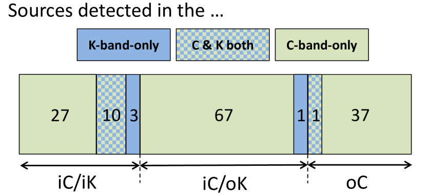
Figure 1: Number of radio continuum sources detected in the K band images (marked in blue and corresponding to 15 sources) and in the C band images (marked in green and corresponding to 142 sources). Out of the 146 detections, only four are detected only in the K band images. The vast majority (131) are detected only in the C band images (see Sect. 3.1 for more details). The bottom labels marked the sources located within the primary beams of the K band and C band images. We find 38 sources located outside the C band primary beam (oC), 68 sources located inside the C band primary beam but outside the K band primary beam (iC/oK) and 40 sources located within the primary beam of both images (iC/iK). See Sects. 3.1 and 3.2 for more details.

Most of the sources (a total of 131) are only detected in the C band image, while four of them are only detected in the K band (see Fig. 1). Only eleven sources are detected at both frequencies. The higher detection rate of sources in the C band is due to several factors. First, four regions were only observed in the C band (see Table 1). This results in 26 radio continuum sources for which we have no access to K band images. Second, the field of view of the C band images (primary beam $\approx$9′) is larger compared to the K band primary beam ($\approx$2′). Only 40 sources are located within the K band primary beam (identified as iC/iK, see Fig. 1). This number reduces to only 24 when considering only the sources that have been observed in both frequency bands. A total of 68 sources are inside the C band primary beam (identified as iC), but outside the K band primary beam (identified as oK, see Fig. 1). The remaining 38 sources are outside the primary beam of the C band observations (marked oC; see also Table LABEL:t:catalogue). The sources that are outside the primary beam are bright enough to be detected even when the telescope’s sensitivity is highly reduced. Thirdly, the spatial filtering of the interferometer is different at both frequencies. In the B-configuration, the VLA recovers scales up to 11″ in the C band, and only up to 4″ in the K band (see also Appendix A of Palau et al. 2010). Finally, one cannot exclude the possibility that some of these sources are extragalactic objects that can only be detected at low frequencies. We have followed the approach of Anglada et al. (1998) to determine the possible contamination of background sources in our catalog. The expected number of background sources $N_{\mathrm{bg}}$ is given by

$$\begin{split}N_{\mathrm{bg}}=&1.4\left\{1-\exp\left[-0.0066\left(\frac{\theta_{F}}{\mathrm{arcmin}}\right)^{2}\left(\frac{\nu}{5\leavevmode\nobreak\ \mathrm{GHz}}\right)^{2}\right]\right\}\\ &\times\left(\frac{S_{0}}{\mathrm{mJy}}\right)^{-0.75}\,\left(\frac{\nu}{5\leavevmode\nobreak\ \mathrm{GHz}}\right)^{-2.52},\end{split}$$ (1)

where $\theta_{F}$ is the area of the sky that has been observed (18 fields in C band, and 14 fields in K band), $\nu$ is the frequency of the observations, and $S_{0}$ is the detectable flux density threshold ($3\times$rms, with an average rms of $22\ \mathrm{\mu Jy\leavevmode\nobreak\ beam^{-1}}$ in the C band, and $30\ \mathrm{\mu Jy\leavevmode\nobreak\ beam^{-1}}$ in the K band). This results in $N_{\mathrm{bg}}=11$ and $N_{\mathrm{bg}}=0.2$ for the C and K band images, respectively. Less than 5% of the sources detected in the C band might be background objects not related to the star-forming regions, while we do not expect contamination in the K band images.

3.2 Spectral index analysis

The spectral index ($\alpha$) is defined as $S_{\nu}\propto\nu^{\alpha}$, where S_ν is the flux density and $\nu$ is the frequency. We have calculated the spectral index for the continuum sources using the measured flux densities at 1.3 cm (K band) and 6 cm (C band). For the sources without detection in one of the bands, we assume an upper limit of flux density equal to $5\sigma$. It should be noted here that the flux densities of the sources were corrected for the primary beam response of the antennas. The sources far away from the phase centers (listed in Table 1) have larger uncertainties in the correction factors of the primary beam and thus, in the final (corrected) flux. Therefore, the sources located within the primary beams in both frequency bands (i.e., sources listed as ‘iC/iK’ in Table LABEL:t:catalogue) have more accurate flux estimates. For the sources outside one of the primary beams (i.e., oK or oC), we do not determine the spectral index because of the high uncertainty involved in the fluxes. In the last column of Table LABEL:t:catalogue we list the calculated spectral indices. For the sources detected at both frequencies, we have improved the determination of the spectral index by creating new images with the same $uv$ (visibility) coverage (see Table 7). This ensures that the interferometer is sensitive to similar spatial scales at both frequencies.

In Fig. 2, we present the spectral index against the flux density to intensity peak ratio for the 24 continuum sources observed at both bands and located within the primary beams. For the sources detected at 6 cm only, we derive an upper limit to the spectral index (see red triangles pointing downwards), while we derive a lower limit for the spectral index for the sources detected only at 1.3 cm, (see blue triangles pointing upwards). The sources detected at both wavelengths (black dots) have a more precise determination of the spectral index. For most sources, we derive spectral indices consistent with thermal emission (i.e., in the range of $-0.1$ to $+2$), and in agreement with observations of other radio jets (e.g., Anglada et al. 2018). Only a few sources show very negative spectral indices (#48, #96 and #144). These sources are likely to be partially filtered out in the K band images, which may result in lower limits for the actual value of the spectral index. In particular, source #48 appears as three distinguishable peaks, which we refer to as a, b, and c, surrounded by a more diffuse and extended structure that is mainly visible in the C band image. It is worth noting that large flux-to-intensity ratios indicate that the source is likely extended and most likely partially filtered out in the K band images, which may result in negative spectral indices.

Figure 2: Spectral index ($\alpha$, see Sect. 3.2) against the flux to intensity ratio for the radio continuum sources detected in both frequency bands and inside the primary beam of both images (sources listed as ‘iC/iK’ in Table LABEL:t:catalogue). The grey-shaded region depicts the spectral index regime associated with thermal free-free emission (i.e., in the range from $-0.1$ to $+2$). Black dots correspond to sources detected in both bands (see spectral indices in Table 3), blue up-pointing triangles correspond to sources detected only in the K band (i.e., lower limits), and red down-pointing triangles correspond to sources detected only in the C band (i.e., upper limits).

Table 2: H₂O and CH₃OH maser features

		R.A. (J2000)	Dec. (J2000)	$V_{\mathrm{maser}}^{\mathrm{a}}$	$V_{\mathrm{LSR}}^{\mathrm{H^{13}CO^{+}}}$	Intensity	Continuum
Region	Maser	(h:m:s)	(°:′:″)	(km s-1)	(km s-1)	(Jy beam-1)	source IDb
IRAS 05358$+$3543	CH3OH	05:39:13.071	$+$35:45:50.938	$-$304	0$-$15.8	00.028	2
G189.78$+$0.34	CH3OH	06:08:35.304	$+$20:39:06.405	0$-$13	00$+$9.2	00.014	14
G192.58$-$0.04	CH3OH	06:12:54.026	$+$17:59:23.060	0$-$14	00$+$9.1	00.720	22
G18.18$-$0.30	H2O	18:25:07.575	$-$13:14:31.487	00$-$3	0$+$50.0	00.570	–
IRAS 18223$-$1243	H2O	18:25:10.804	$-$12:42:26.234	0$+$24	0$+$45.2	00.006	–
IRAS 18228$-$1312	H2O	18:25:41.935	$-$13:10:19.591	0$+$24	0$+$33.1	00.022	48
IRAS 18236$-$1205	H2O	18:26:25.677	$-$12:03:48.402	0$+$28	0$+$26.5	00.010	63
	H2O	18:26:25.575	$-$12:03:48.502	0$+$28	0$+$26.5	00.006	63
	H2O	18:26:25.782	$-$12:03:53.263	0$+$15	0$+$26.5	00.010	64
	H2O	18:26:27.149	$-$12:03:54.888	0$+$15	0$+$26.5	00.014	–
	CH3OH	18:26:25.788	$-$12:03:53.456	00$+$5	0$+$26.5	00.260	64
G19.27$+$0.1M1	H2O	18:25:58.546	$-$12:03:58.516	0$+$28	0$+$26.5	00.022	–
G23.60$+$0.0M1	H2O	18:34:11.237	$-$08:19:07.680	$+$108	$+$106.5	00.440	–
	H2O	18:34:11.452	$-$08:19:07.138	$+$108	$+$106.5	00.100	–
IRAS 18316$-$0602	H2O	18:34:20.918	$-$05:59:41.638	0$+$41	0$+$42.5	11.100	83
	CH3OH	18:34:20.913	$-$05:59:42.087	$-$233	0$+$42.5	00.014	83
G24.33$+$0.1M1	H2O	18:35:08.123	$-$07:35:04.216	$+$108	$+$113.6	04.030	110
	CH3OH	18:35:08.147	$-$07:35:04.260	$-$182	$+$113.6	00.010	110
G24.60$+$0.1M2	H2O	18:35:35.728	$-$07:18:08.796	$+$122	$+$115.3	00.031	–
G24.60$+$0.1M2	H2O	18:35:40.120	$-$07:18:37.417	0$+$54	0$+$53.2	01.020	136
IRAS 19095$+$0930	H2O	19:11:53.975	$+$09:35:50.559	0$+$37	0$+$43.9	26.800	143
	H2O	19:11:53.990	$+$09:35:49.848	0$+$37	0$+$43.9	10.300	143
	CH3OH	19:11:53.993	$+$09:35:50.641	0$+$39	0$+$43.9	00.043	143

3.3 Maser Emission

H₂O and CH₃OH masers are excellent indicators of star formation activity (e.g., Beuther et al. 2002b; Moscadelli et al. 2005; de Villiers et al. 2015). We created image cubes of the H₂O and CH₃OH spectral lines and searched for maser features by scanning the entire velocity range. Despite the limited spectral resolution of our observation setup (see Sect. 2), we found maser emission in 14 of the 18 regions. In Table 4, we list the coordinates of the maser features detected in each region, together with the velocity at which the feature is detected and its intensity. We also compare the velocities of the maser features with the systemic velocities determined from H¹³CO⁺ (1–0) observations (López-Sepulcre et al. 2011). We find that the H₂O masers have velocities that match the H¹³CO⁺ (1–0) velocities, while the CH₃OH masers have a larger discrepancy, probably due to the lower spectral resolution.

The low spectral resolution in our observations compared to the typical maser line widths (a few km s^-1; Elitzur 1982; Kalenskii & Kurtz 2016) leads to smearing of the maser intensities. The intensities given in Table 4 should be considered as lower limits. Despite this limitation, the high-angular resolution of our observations can be used to spatially associate the H₂O and CH₃OH masers to the detected continuum sources. If the angular separation between the continuum source and the maser is smaller than the synthesized beam size (listed in Table 1), we assume that the maser is associated with the continuum source. In the last column of Table 4, we specify the identifier of the continuum source (see Table LABEL:t:catalogue) with which the maser is associated. We find 10 continuum sources associated with maser features (see Section 4.4 for more details).

4 Analysis and discussion

In this section, we determine how many sources in our sample are potential radio jets. For this purpose we study the nature of the detected radio continuum emission, and investigate the association with molecular outflows, masers and EGOs/IRAC 4.5 $\mu$m band and are usually found associated with strong shocks and jets (e.g., Cyganowski et al. 2008, 2009). By using these criteria, we identify the best radio jet candidates in our sample and characterize their properties.

4.1 Nature of the radio continuum emission

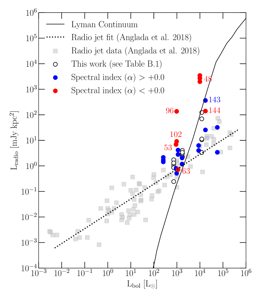
Figure 3: Scatter plot of bolometric luminosity ($L_{\mathrm{bol}}$) and observed radio continuum luminosity ($L_{\mathrm{radio}}$) at 6 cm (C band). Open black circles correspond to the continuum sources detected in our work and located within the primary beam of the K band (1.3 cm) images (i.e., ‘iC/iK’ in Table LABEL:t:catalogue). Blue and red symbols mark the sources with positive and negative spectral indices, respectively, as listed in Table LABEL:t:catalogue and shown in Fig. 2). The solid line represents the values expected from Lyman continuum radiation for a zero-age main-sequence star of a given luminosity (Thompson 1984). The dashed line is a least-squares fit to the radio jets reported by Anglada et al. (2018, shown as grey squares), corresponding to [$L_{\mathrm{radio}}$/mJy kpc²] = $10^{-1.90}$ [$L_{\mathrm{bol}}$/$L_{\odot}$]^+0.59 (see their Eq. 28).

Usually two mechanisms are invoked to explain the origin of thermal free-free radiation from ionized gas in star-forming regions: Photoionization and ionization through shocks (e.g., Gordon & Sorochenko 2002; Kurtz 2005; Sánchez-Monge et al. 2008, 2013c; Anglada et al. 2018). In the case of photoionization, ultraviolet (UV) photons with energies above 13.6 eV are emitted by massive stars and ionize the surrounding atomic hydrogen. In the second scenario, the ionization is produced when ejected material associated with outflows and jets interacts in a shock with neutral and dense material surrounding the forming star (e.g., Curiel et al. 1987, 1989; Anglada et al. 1992).

Anglada (1995, 1996) show that the relation between the radio luminosity and the bolometric luminosity of young stellar objects (YSOs) depends on the origin of the ionization: stellar UV radiation or shocks (see also Anglada et al. 2018). We use this relation to investigate the nature of our continuum sources. The solid line in Fig. 3 shows the maximum radio luminosity that a high-mass object of a given luminosity may have according to its UV radiation, the so-called Lyman continuum limit usually associated with H ii regions. The radio luminosity decreases fast with decreasing bolometric luminosity. In contrast, the radio luminosity originated in shocks (i.e., radio jets) has a less steep curve. The dotted line in Fig. 3 shows the least-squares fit to the sample of radio jets studied in Anglada et al. (2018) and shown as grey squares in the figure.

We have calculated the radio luminosity of our continuum sources as $L_{\mathrm{radio}}=S_{\nu}\,d^{2}$, where $S_{\nu}$ is the observed flux density in the C band (listed in Table LABEL:t:catalogue) and $d$ is the distance to the source (listed in Table 1). The bolometric luminosity ($L_{\mathrm{bol}}$) of each source is uncertain due to the lack of high-resolution data at far-infrared wavelengths. The bolometric luminosity of each region is given in Table A.1 of López-Sepulcre et al. (2011) and provides an upper limit to the actual luminosity. As a simple approach, we divide the bolometric luminosity by the number of radio sources detected within the primary beam to have an estimate of the expected average luminosity for the continuum sources in the region. Circle symbols in Fig. 3 show the continuum sources detected in our work and located inside the K band primary beam (i.e., with reliable flux measurements and listed as iC/iK in Table LABEL:t:catalogue). Colored symbols correspond to those sources for which we could derive the spectral index (see Fig. 2), with blue symbols corresponding to positive spectral indices (i.e., $\alpha>+0.0$, mainly thermal emission) and red symbols corresponding to negative spectral indices. In general, our sources lie in between the two lines defining the radio jet and H ii region regimes. Interestingly, sources with positive spectral indices (blue symbols) seem to preferentially follow, although with some dispersion, the relation found for radio jets, while sources with negative spectral indices (red symbols) are located closer to the Lyman continuum regime. This favours our previous interpretation that sources with negative spectral indices may be slightly extended H ii regions that are partially filtered out in the K band images.

4.2 Association with molecular outflows

We investigate the association of radio continuum sources with molecular outflows by comparing the location of radio sources with respect to the molecular outflow emission reported mainly by López-Sepulcre et al. (2010) and Sánchez-Monge et al. (2013d). It is expected that the most promising radio jet candidates will be in the center of the molecular outflow emission.

We find a total of twenty-four radio continuum sources that are spatially associated with molecular outflow emission (see Table 3 and Fig. 4 for more details). Out of these sources, eighteen (#2, #4, #13, #14, #15, #16, #22, #23, #25, #48a, #48b, #48c, #74, #83, #95, #110, #137 and #143) are located at or near the geometric center of the molecular outflow emission, while the remaining six (#12, #63, #64, #65, #73, and #144) are located within the outflow lobes. Although we cannot confirm that these six sources are at the base of the outflows detected with single-dish telescopes (with angular resolutions of 11–29^″), we cannot exclude that they might drive molecular outflows. Further observations of outflow tracers at higher angular resolution are necessary to confirm and better associated the molecular outflows with the radio continuum sources. In Table 3, we list the outflow momentum rates reported in the literature (see López-Sepulcre et al. 2010; Sánchez-Monge et al. 2013d). For #137, no outflow momentum rate has been reported (Hatchell et al. 2001; Liu et al. 2013).

4.3 Association with EGOs

In this section, we investigate the association of radio continuum sources with Spitzer/IRAC 4.5 $\mu$m emission tracing EGOs, which are considered related to the shocked gas. For the association with EGOs we used the catalogues of Cyganowski et al. (2008, 2009). In total, we found six sources (#42, #63, #64, #119, #137 and #139) with an EGO counterpart (see Table 3).

We have also inspected the Spitzer/IRAC images of the different regions to search for other possible EGOs not included in previous catalogues. We have identified nine radio continuum sources in this category (see sources #48, #65, #73, #74, #83, #110, and #143, marked with a ’?’ symbol in Table 3). The association of these sources with bright 4.5 $\mu$m emission suggests their association with strong shocks and favors the hypothesis of a radio jet origin for the radio continuum emission of these objects. However, a more detailed characterization of the infrared properties of the nine additional sources is necessary to confirm whether these objects are EGOs or not.

Table 3: Properties of the radio jet candidates.

	Flux properties				Source size properties				Outflow/shock activity
ID	$S_{\mathrm{C\leavevmode\nobreak\ band}}$	$S_{\mathrm{K\leavevmode\nobreak\ band}}$	$\alpha$		$\theta_{\mathrm{C\leavevmode\nobreak\ band}}$	$\theta_{\mathrm{K\leavevmode\nobreak\ band}}$	$\beta$		log($\dot{P}_{\mathrm{out}}$)	EGOs	Masers
Radio jet candidates with signposts of outflow activity
002	000.53$\pm$0.01	—	—		¡0.75	—	—		$-3.9\phantom{{}^{\dagger}}$	n	CH3OH
004	000.33$\pm$0.01	—	—		¡1.23	—	—		$-3.9\phantom{{}^{\dagger}}$	n	…
12	000.72$\pm$0.03	—	—		¡0.97	—	—		$-3.1^{\dagger}$	n	…
13	001.24$\pm$0.05	—	—		¡0.75	—	—		$-3.1\phantom{{}^{\dagger}}$	n	…
14	000.69$\pm$0.05	—	—		¡1.08	—	—		$-3.1\phantom{{}^{\dagger}}$	n	CH3OH
15	000.94$\pm$0.04	—	—		¡1.60	—	—		$-3.1\phantom{{}^{\dagger}}$	n	…
16	001.04$\pm$0.04	—	—		¡1.16	—	—		$-3.1\phantom{{}^{\dagger}}$	n	…
22	010.27$\pm$0.22	—	—		¡1.55	—	—		$-3.3\phantom{{}^{\dagger}}$	n	CH3OH
23	01.56 $\pm$0.05	—	—		…	—	—		$-3.3\phantom{{}^{\dagger}}$	n	…
25	00.49 $\pm$0.02	—	—		…	—	—		$-3.3\phantom{{}^{\dagger}}$	n	…
42	004.16$\pm$0.08	…	…		¡0.81	…	…		…	Y	…
48a	055.32$\pm$3.50	015.19$\pm$1.51	$-0.99\pm 0.09$		¡2.70	0¡2.07	¡$-0.20$		$-2.9\phantom{{}^{\dagger}}$	?	H2O
48b	075.41$\pm$9.50	010.53$\pm$1.30	$-1.50\pm 0.14$		¡3.84	0¡1.64	¡$-0.65$		$-2.9\phantom{{}^{\dagger}}$	?	…
48c	129.52$\pm$8.30	054.41$\pm$3.51	$-0.66\pm 0.07$		¡2.28	0¡1.89	¡$-0.14$		$-2.9\phantom{{}^{\dagger}}$	?	…
63	000.99$\pm$0.06	000.75$\pm$0.13	$-0.22\pm 0.07$		¡1.19	0¡1.11	¡$-0.05$		$-2.6^{\dagger}$	Y	H2O
64	000.28$\pm$0.02	000.35$\pm$0.08	$+0.18\pm 0.04$		$<$1.38	0¡0.66	$>-0.56$		$-2.6^{\dagger}$	Y	H2O, CH3OH
65	000.57$\pm$0.14	002.31$\pm$0.09	$+1.08\pm 0.19$		$<$1.46	0$<$0.75	…		$-2.6^{\dagger}$	?	…
73	000.24$\pm$0.15	000.43$\pm$0.09	$+0.45\pm 0.50$		¡0.38	0$<$0.74	$<+0.51$		$-2.4^{\dagger}$	?	…
74	000.35$\pm$0.03	000.49$\pm$0.13	$+0.26\pm 0.21$		¡0.53	0¡0.42	¡$-0.18$		$-2.4\phantom{{}^{\dagger}}$	?	…
83	003.35$\pm$0.21	003.73$\pm$0.29	$+0.08\pm 0.08$		¡0.87	0¡0.85	¡$-0.02$		$-1.8\phantom{{}^{\dagger}}$	?	H2O, CH3OH
95	$<$0.042	000.25$\pm$0.07	$>+1.36$		…	0$<$0.42	…		$-1.8\phantom{{}^{\dagger}}$	n	…
110	000.46$\pm$0.21	001.20$\pm$0.06	$+0.73\pm 0.35$		$<$1.39	0¡0.37	$>-1.01$		$-2.9\phantom{{}^{\dagger}}$	?	H2O, CH3OH
119	001.11$\pm$0.06	$<0.022$	…		¡2.28	…	…		…	Y	…
136	$<$0.10	000.85$\pm$0.12	$>+1.67$		…	0¡1.50	…		…	n	H2O
137	014.40$\pm$1.20	002.21$\pm$0.20	…		¡2.53	0¡1.60	¡$-0.35$		…‡	Y	…
139	000.73$\pm$0.03	$<0.019$	…		¡0.87	…	…		…	Y	…
143	039.50$\pm$1.60	130.87$\pm$2.60	$+1.12\pm 0.04$		¡0.55	0¡0.28	¡$-0.52$		$-3.4\phantom{{}^{\dagger}}$	?	H2O, CH3OH
144	015.57$\pm$0.89	$<$0.32	$<-2.97$		¡2.44	…			$-3.4^{\dagger}$	n	…
Radio continuum sources consistent with positive spectral index, but with no signposts of outflow activity
61	000.14$\pm$0.03	$<$2.10	$<+2.07$		¡1.79	…	…		…	n	…
62	$<$0.05	00.24$\pm$0.09	$>+1.23$		…	0$<$0.44	…		…	n	…
86	000.35$\pm$0.01	$<$2.32	$<+1.43$		$<$1.45	…	…		…	n	…
109	000.08$\pm$0.03	$<$1.75	$<+2.33$		$<$0.94	…	…		…	n	…
113	000.28$\pm$0.01	$<$0.31	$<+0.07$		¡0.85	…	…		…	n	…
126	000.11$\pm$0.01	$<$0.37	$<+0.96$		$<$1.37	…	…		…	n	…
129	000.16$\pm$0.01	$<$0.20	$<+0.18$		¡1.23	…	…		…	n	…
145	002.84$\pm$0.02	$<$4.34	$<+0.32$		$<$1.48	…	…		…	n	…

4.4 Association with masers

Our VLA observations (see Sect. 2.2) allow us to search for H₂O and CH₃OH maser spots associated with radio continuum sources. As shown in Table 4, we have found a total of sixteen H₂O and seven CH₃OH maser spots.

We find ten radio continuum sources associated with maser features, of which three (#2, #14 and #22) are associated with CH₃OH masers only, three sources (#48, #63, and #136) are associated only with H₂O masers, and four sources (#64, #83, #110 and #143) are associated with both types of masers (see Table 3 and Fig. 4). It is worth noting that the three sources associated only with CH₃OH masers correspond to regions observed only in the C band. Future observations of these sources in the K band together with observations of the H₂O maser line could confirm that all sources associated with CH₃OH maser are also associated with H₂O maser features.

The observed Class II 6.7 GHz CH₃OH masers are ideal signposts for embedded young stellar objects and mark the location of deeply embedded massive protostars (e.g., Breen et al. 2013). On the other hand, 22 GHz H₂O masers have been found associated with outflow activity (e.g., Torrelles et al. 2011) as well as tracing disk-like structures around young stellar objects (e.g., Moscadelli et al. 2019). Our maser observations have therefore enabled us to identify at least seven potential candidates for a radio jet (i.e., sources associated with outflow activity).

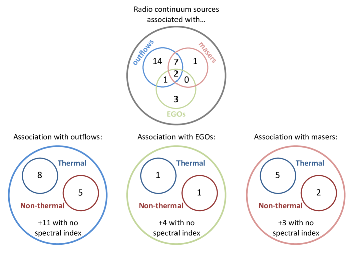
Figure 4: Diagrams summarizing the outflow-activity associations of the radio jet candidates studied in this work. The integer numbers indicate the number radio jet candidates in a specific group (see Table 3). The top diagram summarizes the association of the radio jet candidates with molecular outflows, masers and EGOs (see Sect. 4, for EGOs we only consider association if the source is labeled as ‘Y’ in Table 3). The bottom-row diagrams summarize the results regarding the thermal (spectral index $>-0.1$) and non-thermal (spectral index $<-0.1$) properties of the radio continuum emission. The number of sources for which we could not derive the spectral index is also indicated.

Table 4: Number of the sources with thermal and non-thermal radio continuum emission associated with different outflow activity signatures.

	Non-thermal Sources	Thermal Sources
Outflows	5/5 (100%)	7/8 (88%)
EGOs	1/5 (20%)	1/8 (13%)
Masers (all)	2/5 (40%)	5/8 (63%)
H2O	2/5 (40%)	5/8 (63%)
CH3OH	0/5 (0%)	4/8 (50%)

4.5 Radio jet candidates

Out of the 146 radio continuum sources detected in our study, we have identified twenty-eight sources (see list at the beginning of Table 3) as possible radio jet candidates, based on their association with outflow and shock activity. We find twenty-four of these sources associated with molecular outflow emission, six of them with EGOs, and ten with masers. In the sketch presented in Fig. 4, we summarize these findings.

In addition to these twenty-eight sources, we have also identified eight radio-continuum sources with spectral indices consistent with thermal emission (see bottom list in Table 3). Based on the results shown in Fig. 3, these sources could also be radio jet candidates, despite their lack of association with tracers of outflow and shock activity. In the following, we build on the properties of the identified radio jet candidates.

4.5.1 Radio continuum properties

Reynolds (1986) describe radio jets with a model that assumes a jet of varying temperature, velocity, and ionization fraction. In case of constant temperature, the relations of the flux density ($S_{\nu}$) and source size ($\theta_{\nu}$) with frequency are given by

$$S_{\nu}\propto\nu^{\alpha}=\nu^{1.3-0.7/\epsilon}\\ \mathrm{and}\\ \theta_{\nu}\propto\nu^{\beta}=\nu^{-0.7/\epsilon},$$ (2)

where $\epsilon$ depends only on the geometry of the jet and is the power-law index that describes how the width of the jet varies with the distance from the central object. In this model, the spectral index $\alpha$ is always smaller than 1.3 and drops to values $<0.6$ for confined jets ($\epsilon<1$; Anglada et al. 1998).

In Table 3, we list the spectral index ($\alpha$) and the source size index ($\beta$) for our radio jet candidates. The latter only for the sources detected at both frequencies. Nine of the radio jet candidates associated with outflow/shock activity have spectral indices consistent with thermal emission ($>-0.1$), with six showing clear positive ($>+0.4$) spectral indices. These values are consistent with the model of Reynolds (1986) for values of $\epsilon>0.6$. For such geometries of the jet, the source size index ($\beta$) is expected to be about $-1$. The source size indices reported in Table 3 are mainly in the range $-0.1$ to $-1.0$, in agreement with the model of Reynolds (1986) for radio jets.

Despite most of our radio jet candidates have spectral indices consistent with thermal emission (64% of the sample, see Table 3), we find some sources (accounting for 36% of the sample, five sources) that show negative spectral indices. This finding is in agreement with some recent works. For example, Moscadelli et al. (2016) find about 20% of their sample of 15 radio continuum sources to be associated with non-thermal emission. The presence of non-thermal emission is explained in terms of synchrotron emission from relativistic electrons accelerated in strong shocks within the jets, and a number of cases have been studied in more detail (e.g., Carrasco-González et al. 2010; Sanna et al. 2019). Further detailed observations towards these new four non-thermal radio jet candidates, can provide further constraints to understand the characteristics of this kind of objects.

We have searched for possible relations between the presence of thermal and non-thermal radio jets and different outflow/shock activity signposts (i.e., outflows, masers and EGOs). We summarize our findings in the bottom panels of Fig. 4). We do not find a preferred relation between thermal and non-thermal radio jets with the outflow activity signposts, since we find similar percentages (see Table 4) for the association with outflows (88% and 100%, respectively), EGOs (13% and 20%), and masers (55% and 40%). The low number of objects included in our analysis prevents us from deriving further conclusions, and we indicate that a larger sample of radio jets needs to be studied to better understand the properties and differences between thermal and non-thermal radio jets. It is also worth noting that all the four objects associated with both CH₃OH and H₂O masers are thermal radio jet candidates (see Table 3), while only one of the three objects associated with only H₂O masers shows thermal emission. This might suggest that radio jets associated with CH₃OH masers tend to have positive spectral indices (i.e., thermal emission), while radio jets associated with only H₂O masers might preferentially have negative spectral indices (i.e., non-thermal emission). However, the low number of sources studied in our sample prevents from deriving further conclusions. One should also note that the different levels of association of the radio continuum sources with maser emission may be affected by the variability of masers (Felli et al. 2007; Sugiyama et al. 2017; Ashimbaeva et al. 2017). Moreover, we can not discard that the poor spectral resolution of our observations, which may smear out the intensity of the maser lines making some of them undetectable with our sensitivity limits, may also affect our detectability limits. Despite these limitations, our results are in agreement with the 6.7 GHz CH₃OH masers tracing the actual location of the newly-born YSOs usually associated with thermal winds/jets, while H₂O masers may be originated in strong shocks where non-thermal synchrotron emission can be relevant (see e.g., Moscadelli et al. 2013, 2016).

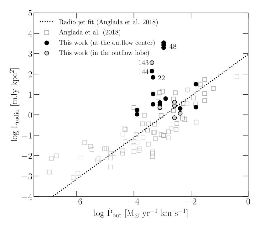
Figure 5: Relation between radio luminosity ($L_{\mathrm{radio}}$) and outflow momentum rate ($\dot{P}_{\mathrm{out}}$). Open boxes show data from (Anglada et al. 2018, see also Anglada et al. 1992). The dashed line is a least-squares fit to the radio jets reported by Anglada et al. (2018), corresponding to [$L_{\mathrm{radio}}$/mJy kpc²] = 10^+2.97 [$\dot{P}$/$M_{\odot}$ yr^-1 km s^-1]^+1.02 (see their Eq. 31).

4.5.2 Jet-outflow connection

It has been found that the radio luminosity ($L_{\mathrm{rad}}=S_{\nu}d^{2}$) of thermal radio jets is correlated with the energetics of the associated molecular outflows. The relationship between radio luminosity and momentum rate in the outflow ($\dot{P}_{\mathrm{out}}$) is empirically derived by Anglada et al. (1992, see also ). In Fig. 5, we compare our radio jet candidates (see Table 3) with the radio jets studied by Anglada et al. (2018). As reported by Anglada et al. (2018), there is a tight correlation between the radio luminosity of the jet and the outflow momentum rate. This relationship is interpreted as proof that shocks are the ionization mechanism of radio jets (see e.g., Rodríguez et al. 2008; Anglada et al. 2018). Most of the radio jet candidates investigated in this work, with the exception of only a few sources, follow this relationship, suggesting a radio jet origin for the detected radio continuum emission. The exceptions are mainly the sources #48a, #48b, #48c, #143 and #144, which have a much larger radio luminosity compared to the associated outflow momentum rate. This excess suggests that another mechanism could be responsible for a large fraction of the observed radio continuum emission. Based on the location of these sources in the diagram shown in Fig. 3, these sources may correspond to more evolved and extended H ii regions, instead of radio jets, thus explaining the discrepancy between the observed radio luminosity and outflow momentum rate. In this case, we could be facing two possible scenarios. The first is that the sources are indeed radio jets transitioning into a more evolved H ii region phase (similar to what has been proposed for G35.20$-$0.74N, Beltrán et al. 2016). The second scenario is that the radio continuum sources that we are detecting are only associated with an H ii region, and the spatial coincidence with the molecular outflow emission is due to the presence of another (lower-mass) object powering the outflow but with non-detectable radio continuum emission in our maps. Higher angular resolution observations of the molecular outflow can better establish the location of the powering source and its association with the detected radio continuum sources.

Following Eq. 8 of Anglada et al. (2018, see also ), we estimate the ionized mass-loss rate ($\dot{M}_{\mathrm{ion}}$) of our radio jet candidates as

$$\begin{split}\left(\frac{\dot{M}_{\mathrm{ion}}}{10^{-6}\leavevmode\nobreak\ M_{\sun}\leavevmode\nobreak\ \mathrm{yr}^{-1}}\right)=&0.108\left(\frac{d}{\mathrm{kpc}}\right)^{1.5}\left[\frac{\left(2-\alpha\right)\left(0.1+\alpha\right)}{1.3-\alpha}\right]^{0.75}\\ &\times\left(\frac{T}{10^{4}\leavevmode\nobreak\ \mathrm{K}}\right)^{-0.075}\left[\left(\frac{S_{\nu}}{\mathrm{mJy}}\right)\left(\frac{\nu}{10\leavevmode\nobreak\ \mathrm{GHz}}\right)^{-\alpha}\right]^{0.75}\\ &\times\left(\frac{V_{\mathrm{jet}}}{200\leavevmode\nobreak\ \mathrm{km}\leavevmode\nobreak\ \mathrm{s}^{-1}}\right)\left(\frac{\nu_{m}}{10\leavevmode\nobreak\ \mathrm{GHz}}\right)^{0.75\alpha-0.45}\\ &\times\left(\frac{\theta_{0}}{\mathrm{rad}}\right)^{0.75}(\sin\leavevmode\nobreak\ i)^{-0.25},\end{split}$$ (3)

where $\alpha$ is the spectral index and $S_{\nu}$ is the radio continuum flux, both listed in Table 3, and $d$ is the distance to the source. The opening angle of the jet $\theta_{0}$ can be approximated as $2\arctan(\theta_{\mathrm{min}}/\theta_{\mathrm{maj}})$ (Beltrán et al. 2001; Anglada et al. 2018). We assume a value of 0.5 for the ratio of the minor and major axis of the jet. We also assume that the velocity of the jet ($V_{\mathrm{jet}}$) is 500 km s^-1 and that it lies in the plane of the sky (i.e., $\sin\leavevmode\nobreak\ i=1$). For a random orientation of the jet on the celestial plane, the value of $\sin\leavevmode\nobreak\ i$ is on average $\pi/4$ (e.g., Beltrán et al. 2001). Usually, a value of $T=10^{4}$ K is adopted for ionized gas. For the turnover frequency $\nu_{m}$, we assume a value of 40 GHz (see discussion in Anglada et al. 2018). In Fig. 6, we show the relationship between the mass loss rates of the ionized and the molecular outflow for the thermal radio jet candidates listed in Table 3 and associated with the molecular outflows. Major uncertainties in the determination of $\dot{M}_{\mathrm{ion}}$ may arise from parameters such as the jet velocity, the turnover frequency or the aspect ratio of the jet, as they cannot be determined from our observational data. However, their effects are almost negligible and variations within reasonable ranges result in variations of the ionized mass loss rate of less than a factor of 10. Our derived $\dot{M}_{\mathrm{ion}}$ are mainly in the range of $10^{-7}$ to $10^{-5}$ $M_{\odot}$ yr^-1, consistent with the values reported for low-mass radio jets ($\approx 10^{-10}$ $M_{\odot}$ yr^-1) and high-mass radio jets ($\approx 10^{-5}$ $M_{\odot}$ yr^-1, see Rodriguez et al. 1994; Beltrán et al. 2001; Guzmán et al. 2010, 2012). The dashed lines in Fig. 6 indicate different degrees of ionization for the mass loss rate. Most of our radio jet candidates, with the exception of source #143, which is probably associated with an already developed H ii region (see Fig. 5 and discussion above), have ionization levels of $\dot{M}_{\mathrm{ion}}$ = 10^-3 $\times$ $\dot{M}_{\mathrm{out}}$. These values are about one to two orders of magnitude smaller than those reported in previous studies (see e.g., Rodriguez et al. 1990; Hartigan et al. 1994; Bacciotti et al. 1995; Anglada et al. 2018). This difference may be due to uncertainties in the assumed parameters of Eq. 3, as well as to the fact that our molecular outflow emission is studied with a single-dish (sensitive to all scale structures), while the radio jet observations were carried out with a large interferometric configuration likely resolving out part of the radio jet emission.

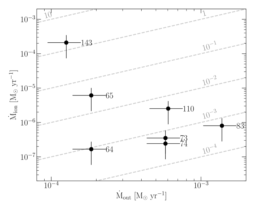
Figure 6: Relation between ionized ($\dot{M}_{\mathrm{ion}}$) and molecular outflow ($\dot{M}_{\mathrm{out}}$) mass loss rates for the radio jet candidates listed in Table 3. The ionized mass loss rate is derived for the thermal radio jets using Eq. 3, while the molecular outflow mass loss rate is provided in López-Sepulcre et al. (2010) and Sánchez-Monge et al. (2013d). The dashed lines indicate different ionization levels given by the ratio $\dot{M}_{\mathrm{ion}}$ to $\dot{M}_{\mathrm{out}}$.

4.5.3 Best radio jet candidates

In previous sections, we have analyzed the properties of the 146 detected radio continuum sources and built a sample of possible radio jet candidates based on their association with outflow activity: molecular outflows, EGOs, and masers (see Table 3). In Sect. 4.5.1 and 4.5.2, we have investigated in more detail the possible nature of the radio continuum emission and its relation to the outflow activity tracers, in particular, the outflow momentum rate. The results presented in Figs. 3 and 5 allow us to identify sources with properties that differ from those expected from radio jets, therefore suggesting that these sources may actually not be radio jets. From this analysis and the individual description of selected sources (see Appendix A), we discuss in this section which objects are most likely to be radio jets.

Out of the 28 sources listed in Table 3, five of them have radio luminosities similar to those expected for H ii regions: #48a, #48b, #48c, #143 and #144 (see Fig. 3). In addition, all of these sources, with the exception of #143, have negative spectral indices. These negative values could be due to the sources being slightly extended (as expected for H ii regions) and partially filtered out in the K band images. Moreover, these five sources also exhibit large radio luminosities compared to their associated outflow momentum rates (see Fig. 5), which supports the interpretation that there may be an excess of radio continuum emission not necessarily associated with a radio jet, but with an H ii region. In the absence of further evidence, we are not in a position to interpret further and we can not consider these sources to be among the best radio jet candidates. Further observations, sensitive to extended emission, can provide the necessary information to better characterize these sources in terms of their spatial extend and the nature of the emission. It is also worth noting that sources with negative spectral indices could correspond to background sources with synchrotron radiation since we expect about 11 objects in our sample to have this possible origin (see Sect. 3.1). Source #22 also shows an excess of radio-continuum emission compared to its outflow momentum rate, which suggests that this is also a dubious radio jet candidate. From the individual source descriptions presented in Appendix A, sources #42 and #137 seem to be radio continuum sources with most of their emission dominated by cometary/ultracompact H ii regions, which makes it difficult to identify a radio jet in our data.

Out of the remaining sources listed in Table 3, we can identify seven of them having a high probability to be radio jets. These are sources #2, #14, #22, #64, #74, #83 and #110, which are associated with additional outflow/shock activity such as masers and EGOs. One should note that source #74 is adjacent to two H₂O maser features, which are only 2″ away and coincident with extended 4.5 $\mu$m emission (see Fig. 13). The remaining sources do still classify as radio jet candidates, since we do not have clear evidence against that. Some of them are located at the center of molecular outflows (e.g., #95) but are not associated with additional outflow/shock signposts. This could be related to the variability of H₂O masers (see Sect. 4.5.1). Others are located within molecular outflow lobes (e.g., #12, #63, #64, #65, #73, and #144), and for which higher angular resolution observations of outflow tracers are necessary to confirm if they are powering some of the molecular outflows. Other sources, despite not being associated with molecular outflows, show other shock activity signposts such as the presence of EGOs (e.g., #119, #136, #139). Further observational constrains are therefore needed to fully confirm or discard these objects as radio jets. The results acquired so far, allow us to classify them as radio jet candidates.

5 Implications for high-mass star formation

Recently, Rosero et al. (2019) studied the properties of 70 radio continuum sources associated with the earliest stages of high-mass star formation. They find that $\approx$30–50% of their sample are ionized jets. This fraction is in agreement with our findings. Out of the 146 radio continuum sources detected in our study, we identify 28 possible radio jets (i.e., about 19% of our sample). However, if we focus on the sources for which we have more accurate information (i.e., sources classified as iC/iK in Table LABEL:t:catalogue, see also Sect. 3.1), we have 24 out of 40 sources being potential radio jets. Therefore, the percentage of radio continuum sources being radio jets increases up 60%. This suggests that about half of the radio continuum sources found in star-forming regions at early evolutionary stages may indeed be radio jets powered by young stars. The remaining $\approx$50% of objects could still be radio jets for which we have not yet identified shock activity signposts, or they could represent extremely compact H ii regions in their early stages of development. These objects could be powered by early B-type stars and not necessarily by the most massive stars, and could be an intermediate stage between radio jets and already developed H ii regions (see e.g., Beltrán et al. 2016; Rivera-Soto et al. 2020).

López-Sepulcre et al. (2010) classified the regions studied in our work as infrared dark (IRDC, infrared dark cloud) and infrared bright (HMSFR, high-mass star-forming region) based on their detectable infrared emission. Our sample, therefore, consists of two sub-classes: IRDC (8 regions) and HMSFR (10 regions; see Table 1). We assume that these two types belong to different evolutionary phases of massive star formation, with the IRDC regions being less evolved than the HMSRF regions. Considering the 40 sources located within the primary beam of our images (i.e., sources classified as iC/iK), we find $\approx$2.8 radio continuum sources per HMSFR region, and $\approx$1.8 radio continuum sources per IRDC region. This suggests that it is more probable to detect compact radio continuum emission in more evolved regions. Regarding the presence of radio jets in these two evolutionary stages, we find 21 out of the 28 radio jet candidates listed in Table 3 in HMSFR regions (corresponding to 75%), while we only find 7 (corresponding to 25%) in the less evolved IRDC regions. If we consider only the best radio jet candidates (see Sect. 4.5.3), we find five radio jets (#2, #14, #22, #64 and #83; corresponding to 71%) in HMSRF regions and two radio jets (#74 and #110; corresponding to 29%) in IRDC regions. This shows a preference of radio jets to be found in more evolved clouds. Complementary to this, we can determine the fraction of IRDC and HMSFR regions that harbor radio jets. Out of the 8 IRDC regions studied in this work, only 2 (corresponding to 25%) harbor one of the best radio jet candidates. This increases up to 50% (5 out of 10) for the HMSFR regions. Therefore, the frequency of radio jets in IRDC regions is lower than in HMSFR regions. One possible explanation is that the jets may become larger and brighter with time. Our limited data do not show that IRDC jets are smaller or fainter than HMSFR jets, but future work on larger source samples may provide further insight.

6 Summary

In this work, we have used of the VLA in two different bands (C and K band, corresponding to 6 and 1.3 cm wavelengths) to search for radio jets powered by high-mass YSOs. We have studied a sample of 18 high-mass star-forming regions with signposts of SiO and HCO⁺ outflow activity. In the following we summarize our main results.

• We have identified 146 radio continuum sources in the 18 high-mass star forming regions, with 40 of the radio continuum sources located within the primary beams of our images (i.e., labeled as iC/iK and with reliable flux measurements). Out of these sources, 131 (27 iC/iKs) are only detected in the C band, 4 (3 iC/iKs) are only detected in the K band, and 11 (10 iC/iKs) are detected in both bands. This different detection level is likely due to different factors: (i) four regions were not observed in the K band, (ii) the C band images have a larger field of view, and (iii) the K band images are affected by a larger interferometric spatial filtering. In addition to the continuum emission, we have detected 23 maser features in the 6.7 GHz CH₃OH and 22 GHz H₂O lines.

• Out of the 146 continuum sources, only 40 sources are located within the field of view of both images allowing for an accurate characterization of their radio properties. For these sources we have derived the spectral index, which we find to be consistent with thermal emission (i.e., in the range $-$0.1 to $+$2.0) for most of the objects (73%).

• We have investigated the nature of the radio continuum emission by comparing the radio luminosity to the bolometric luminosity. We find that most sources with positive spectral indices (i.e., thermal emission) follow the trend expected for radio jets, while sources with large negative spectral indices seem to follow the relation expected for H ii regions. These large negative spectral indices are likely due to the emission in the K band images being partially filtered out.

• Based on the association of the radio continuum sources with shock activity signposts (i.e., association with molecular outflows, EGOs or masers), we have compiled a list of 28 radio jet candidates. This corresponds to $\approx$60% of the radio continuum sources located within the field of view of both VLA images. Out of these sample of radio jet candidates, we have identified 7 objects (#2, #14, #22, #64, #74, #83, and #110) as the most probable radio jets. The remaining 21 require additional observations, either at different radio frequency bands or of molecular outflow tracers at higher resolution, to confirm or discard them as radio jets.

• We find about 7–36% of the possible radio jet candidates to show non-thermal radio continuum emission. This is consistent with previous studies reporting $\approx$20% of non-thermal radio jets. We do not find a clear association of the non-thermal emission with the presence of outflows, EGOs or masers. However, and despite the low statistics, we find that radio jet candidates associated with CH₃OH masers have thermal emission, while those radio jet candidates associated with only H₂O masers tend to have non-thermal emission. This is in agreement with the 6.7 GHz CH₃OH masers tracing the actual location of newly-born YSOs powering thermal winds and jets, while the H₂O masers may be originated in strong shocks where non-thermal emission becomes relevant.

• As previously found in other works, we find a correlation between the radio luminosity of our radio jet candidates and their associated outflow momentum rates. We derive an ionized mass loss rate in the range $10^{-7}$ to $10^{-5}$ $M_{\odot}$ yr^-1, which results in ionization levels of $\dot{M}_{\mathrm{ion}}=10^{-3}\leavevmode\nobreak\ \dot{M}_{\mathrm{out}}$ (i.e., $\approx$0.1% of the outflow mass being ionized).

• The 18 high-mass star-forming regions studied in this work are classified in two different evolutionary stages: 8 less evolved IRDC and 10 more evolved HMSFR. We find more radio continuum sources ($\approx$2.8 sources per region) in the more evolved HMSFR compared to the IRDC ($\approx$1.8). Regarding radio jets, we find about 71% of the radio jet candidates to be located in HMSFR regions, and only 29% in IRDC regions. Complemenary to this, 25% of the IRDC regions harbor one of the most probable radio jet candidates, while this percentage increases up to 50% for the HMSFR regions. This suggests that the frequency of radio jets in the less evolved IRDC regions is lower compared to the more evolved HMSFR regions.

Appendix A Comments on individual sources

In the following, we comment on different aspects of selected sources for which additional literature information is available.

IRAS 05358$+$3543 (#2 and #4)

In region IRAS 05358$+$3543, we have identified two radio continuum sources that can be potential radio jets (see Fig. 7). Sources #2 and #4 were observed only in the C band, and therefore we cannot determine a spectral index for these sources. Despite this limitation, both sources are located at the center of the molecular outflow reported by López-Sepulcre et al. (2010). Furthermore, source #2 is associated with a 6.7 GHz CH₃OH maser emission, suggesting that this marks the position of a massive YSO. Of the two radio continuum sources, source #2 is likely the main object powering the molecular outflow for which its centimeter emission traces a radio jet. Further observations at different frequency bands are necessary to better constrain its properties.

G189.78$+$0.34 (#12, #13, #14, #15 and #16)

In region G189.78+0.34, we have identified five radio continuum sources (sources #12 to #16) associated with the molecular outflow reported by López-Sepulcre et al. (2010). All of them are located at the center of the outflow, with source #12 slightly offset from the rest (see Fig. 8). All these sources were observed only in the C band and no spectral index can be derived. Out of the five sources, source #14 is associated with CH₃OH maser emission (see also Caswell et al. 2010) suggesting that this marks the location of a massive YSO. The radio continuum sources are found in an elongated chain extending from the south-east to the north-west. This direction is consistent with the orientation of the molecular outflow (López-Sepulcre et al. 2010). Overall, we consider that source #14 is the powering source and most likely the main component of the radio jet. The other sources could correspond to different radio continuum knots located along the jet, as seen in other sources (e.g., HH 80-81: Carrasco-González et al. 2010, and G35.20$-$0.74 N: Beltrán et al. 2016), where the radio continuum knots usually show non-thermal spectral indices. Observations at different frequency bands are necessary to gather information on the spectral index and thermal/non-thermal nature of the different radio continuum sources in the region.

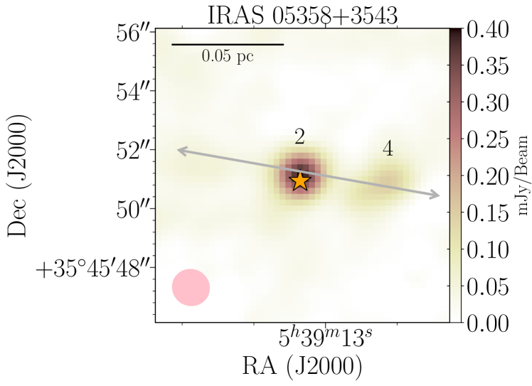
Figure 7: VLA C band (6 cm) continuum emission map of the radio jet candidates #2 and #4 located in the region IRAS 05358$+$3543. The pink ellipse is the beam size of the C band. The orange star marks the location of the CH₃OH maser (see Table 4). The grey double-headed arrow indicates the direction of the outflows.

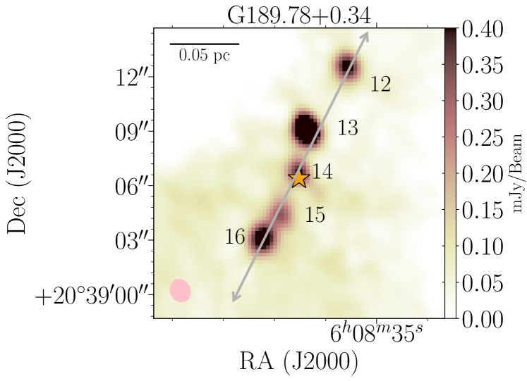
Figure 8: VLA C band (6 cm) continuum emission map of the radio jet candidates #12, #13, #14, #15 and #16 located in the region G189.78$+$0.34. The pink ellipse is the beam size of the C band. The orange star marks the location of the CH₃OH maser (see Table 4). The grey double-headed arrow indicates the direction of the outflows.

G192.58$-$0.04 (#22, #23 and #25)

In region G192.58$-$0.04, we have identified sources #22, #23, and #25 as potential radio jets (see Fig. 9). These sources were observed only in the C band and no spectral index can be derived. Out of the three sources, source #22 is associated with CH₃OH maser emission suggesting that this source may mark the location of a massive YSO. The sources are located at the center of the molecular outflow reported by López-Sepulcre et al. (2010). Out of the three sources, we consider that source #22 is the most probable radio jet. The comparison between the radio continuum luminosity with the outflow momentum rate (see Fig. 5), also confirms this possibility, although there seems to be a slightly excess of radio continuum emission, suggesting that there can be an additional contribution to the radio continuum source (e.g., from an early-stage H ii region).

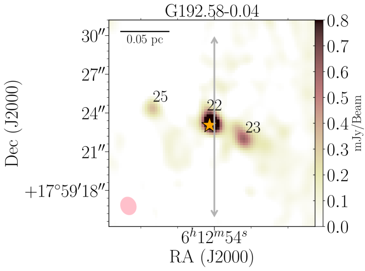
Figure 9: VLA C band (6 cm) continuum emission map of the radio jet candidates #22, #23 and #25 located in the region G192.58$-$0.04. The pink ellipse is the beam size of the C band. The orange star marks the location of the CH₃OH maser (see Table 4). The grey double-headed arrow indicates the direction of the outflows.

IRAS 18223$-$1243 (#42)

In the region IRAS 18223$-$1243, we identified the radio continuum source #42 (see Fig. 10) as adjacent to the one reported in Cyganowski et al. (2011) EGO F G18.67$+$0.03$-$CM1. This is the only signposts of shock activity, since no molecular outflow or maser emission are found for this object. In addition, Cyganowski et al. (2012) report the existence of a massive protocluster consisting of a hot molecular core and an ultracompact H ii region. Our source seems to be located at the same position of the ultracompact H ii region, which makes us to doubt if this can be a radio jet candidate.

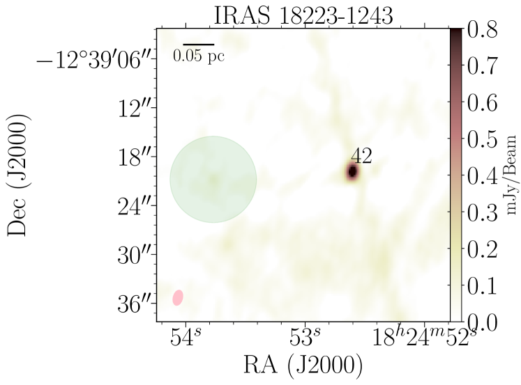
Figure 10: VLA C band (6 cm) continuum emission map of the radio jet candidate #42 located in the region IRAS 18223$-$1243. The pink ellipse is the beam size of the C band. The green circle with a radius of $\sim$5^″ marks the EGO F G18.67$+$0.03-CM1 reported by Cyganowski et al. (2011).

IRAS 18228$-$1312 (#48)

Radio continuum source #48 is observed as a group of three compact sources (#48a, #48b and #48c) surrounded by an extended and more diffuse structure. One of these compact sources (#48a) is clearly associated with H₂O maser emission (see Fig. 11). The Spitzer/IRAC 4.5 $\mu$m emission is extended and spatially coincident with the radio continuum extended emission. The spectral indices for these three compact sources are in the range $-0.6$ to $-1.5$, most likely due to additional filtering of the emission in the K band image. Previous studies have classified this extended source as a region containing hypercompact (HC) and ultracompact (UC) H ii regions (e.g., Chini et al. 1987; Lockman 1989; Kurtz et al. 1994; Kuchar & Clark 1997; Leto et al. 2009), which is consistent with our derived radio continuum luminosity (see Figs. 3 and 5). It is worth noting that the the three sources are spatially located at the center of a molecular outflow (e.g., López-Sepulcre et al. 2010). This may suggest that one of the compact sources may be powering the molecular outflow. In this case, this object would be in a evolutionary stage where the radio jet still exists but a young H ii region has already developed, similar to the high-mass young stellar object G35.20$-$0.74 N (e.g, Sánchez-Monge et al. 2013b, 2014; Beltrán et al. 2016).

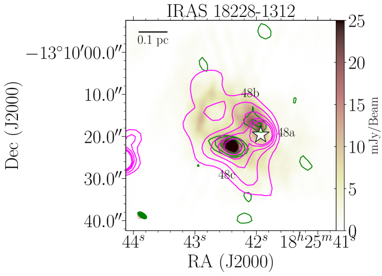
Figure 11: VLA C band (6 cm) continuum emission map of source #48 located in the region IRAS 18228$-$1312. Three bright peaks are visible and labelled as #48a, #48b and #48c. The green contour levels of the K band (1.3 cm) continuum emission are 3, 5 and 9 times 0.7 mJy beam^-1. The magenta contours show the Spitzer/GLIMPSE 4.5 $\mu$m emission. The pink and green ellipses are the beam sizes of the C and K bands, respectively. The white star marks the location of the H₂O maser (see Table 4).

IRAS 18236$-$1205 (#63, #64 and #65)

We have identified nine radio continuum sources in the IRAS 18236$-$1205 region (also referred to in the literature as G19.36$-$0.03), three of which have been classified as radio jet candidates: Sources #63, #64 and #65 with spectral indices of $-0.22\pm 0.07$, $+0.18\pm 0.04$ and $+1.08\pm 0.19$. We have identified four H₂O maser features near these sources (see Fig. 12). Two maser features are associated with source #63, one maser feature is associated with source #64 (which also spatially coincides with a CH₃OH maser), and the last maser feature is located in the center of the red-shifted outflow lobe where no radio continuum emission is detected. The molecular outflow in this region has been mapped in the lines SiO (2–1) and HCO⁺ (1–0) by (Sánchez-Monge et al. 2013d).

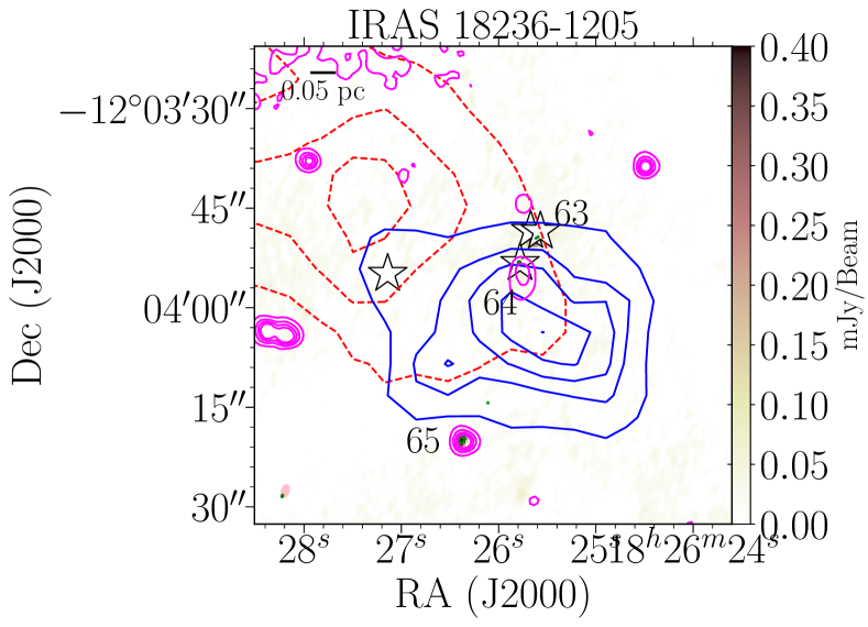
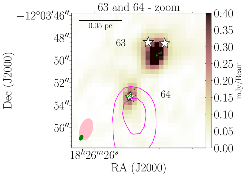
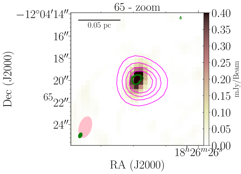
Figure 12: VLA C band (6 cm) continuum emission map of the radio jet candidates #63, #64 and #65 located in the region IRAS 18236$-$1205. A close-up view of the three radio sources is shown in the bottom and right panels. The green contour levels of the K band (1.3 cm) continuum emission are 3, 5 and 7 times 30 $\mu$Jy beam^-1. The magenta contours show the Spitzer/GLIMPSE 4.5 $\mu$m emission. The blue- and red-shifted outflow lobed of SiO (2$-$1) are shown as blue-solid and red-dashed contours, respectively (see Sánchez-Monge et al. 2013d). The pink and green ellipses are the beam sizes of the C and K bands, respectively. The white stars mark the location of the H₂O masers (see Table 4).

Sources #63 and #64 are associated with EGOs (see Cyganowski et al. 2009), indicating the presence of strong shock activity in these two sources. Their location near the center of the molecular outflow together with their association with H₂O maser emission and EGOs, suggests that these two sources could be candidates for radio jets. The source #64 is spatially more coincident with the geometric center of the outflow, and its association with 6.7 GHz CH₃OH maser emission, suggests that a massive YSO exists at this position. This massive YSO could be the driving source of the molecular outflow seen on larger scales. The third candidate (source #65) is located $\sim$28$\arcsec$ away from the source #64 and the center of the outflow, and has been studied by (Cyganowski et al. 2011, G19.36-0.03-CM2). This source is associated with an emission of 4.5 $\mu$m, although it is unclear whether it can be convincingly classified as an EGO (Cyganowski et al. 2009). The positive spectral index indicates the presence of thermal emission, which could come from a radio jet. However, there is no clear evidence of outflow or shock activity. The source #65 is also located in the vicinity of a dense core (18236$-$1205 P8) identified by Lu et al. (2014) in the VLA NH₃ maps, which supports the interpretation of this source as an embedded young stellar object. Overall, the source #65 could be a YSO-powered radio jet in the vicinity of the more massive object (sources #63 and #64) in IRAS 18236$-$1205.

G23.60$+$0.0M1 (#73 and #74)

The G23.60$+$0.01M1 star-forming region has been studied in the literature by various authors (e.g., Rathborne et al. 2006; Battersby et al. 2010; Ginsburg et al. 2013), who reported the presence of two massive dense clumps with masses of 100 $M_{\odot}$ and 120 $M_{\odot}$. The two candidate radio jets (#73 and #74) have positive spectral indices consistent with thermal emission of radio jets. In particular, the source #74 is located at the center of the molecular outflow reported by Sánchez-Monge et al. (2013d) and is associated with a strong 4.5 $\mu$m emission (see Fig. 13). The two H₂O maser detected in the region are slightly displaced from the radio continuum source but coincide with the extended 4.5 $\mu$m emission (see Fig. 13-bottom). The association of molecular outflow emission, bright and extended 4.5 $\mu$m emission, and close H₂O maser features favor the interpretation of this source is a good radio jet candidate.

The second radio continuum source (#73) is located relatively close to the center of the outflow. However, no maser or EGOs are found in connection with the source. Although we cannot reject this source as a radio jet, we prefer the source #74 as the main object driving the outflow observed in the region.

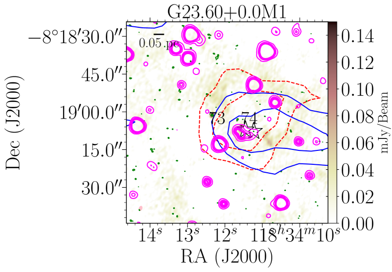
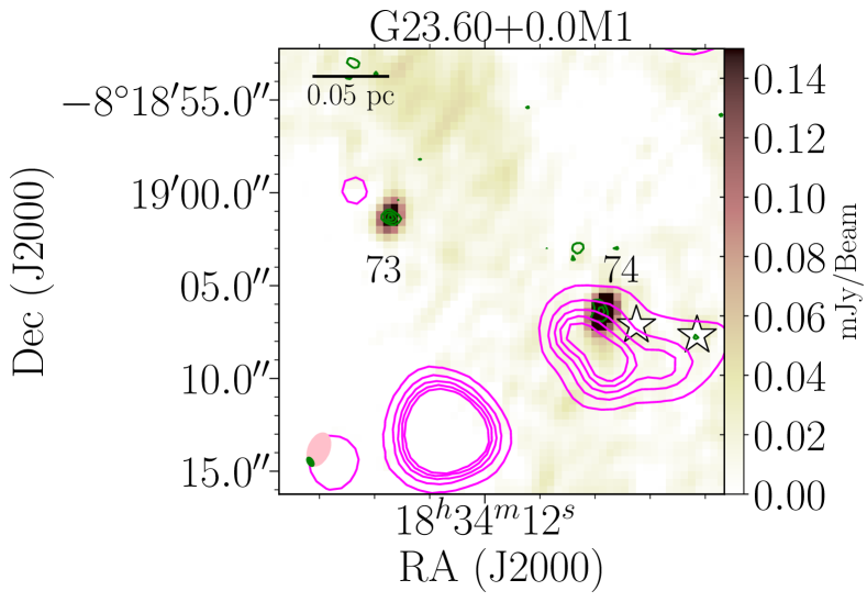
Figure 13: VLA C band (6 cm) continuum emission map of the radio jet candidates #73 and #74 located in the region G23.60$+$0.0M1. A close-up view of the two radio sources is shown in the bottom panel. The green contour levels of the K band (1.3 cm) continuum emission are 3, 5, 7, 9 and 11 times 20 $\mu$Jy beam^-1. The magenta contours show the Spitzer/GLIMPSE 4.5 $\mu$m emission. The blue- and red-shifted outflow lobed of SiO (2$-$1) are shown as blue-solid and red-dashed contours, respectively (see Sánchez-Monge et al. 2013d). The pink and green ellipses are the beam sizes of the C and K bands, respectively. The white stars mark the location of the H₂O masers (see Table 4).

IRAS 18316$-$0602 (#83 and #95)

We have identified thirteen radio continuum sources in the IRAS 18316$-$0602 region, two of which have been classified as radio jet candidates: Sources #83 and #95. The source #83 has an almost flat spectral index ($0.08\pm 0.08$) and shows a weak extension to the south, which is better resolved in the K band image. Source #95 is fainter, appears located about 3″to the south-east of source #83, and is visible only in the K band (some faint emission slightly above the noise level is visible in the C band image, see Fig. 14). As for the maser emission, we have identified both a H₂O and a CH₃OH maser feature associated with the brightest source #83. This source has been studied in previous works (e.g., Roueff et al. 2006; Cutri & et al. 2012; Azatyan et al. 2016; Stecklum et al. 2017), in some of them named RAFGL 7009S. The source is detected in the near-infrared together with two other objects separated by about 10″, and surrounded by a diffuse and extended structure (see e.g., Stecklum et al. 2017).

López-Sepulcre et al. (2010) and Sánchez-Monge et al. (2013d) report on molecular outflow emission in the region. The blue and red contours in Fig. 14 show the SiO (2–1) blue-shifted and red-shifted outflow emission. Both radio continuum sources (#83 and #95) are located close to the center of the outflow. Although this region was not included in the Cyganowski et al. (2008, 2009, 2011) surveys, we have identified a bright 4.5 $\mu$m source in the Spitzer/GLIMPSE data. However, the source is located at the edge of the area surveyed by Spitzer, which prevents a detailed characterization of its infrared emission. The association of the source #83 with a 6.7 GHz CH₃OH maser emission suggests that this source harbors a massive YSO together with its central location within the outflow and its association with a H₂O maser feature hints towards this source is the radio jet that drives the outflow. The almost flat spectral index may indicate that this is a fully ionized radio jet. However, further observations in different frequency bands may help to better narrow down the spectral index and the status of radio continuum emission.

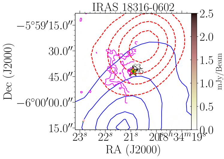
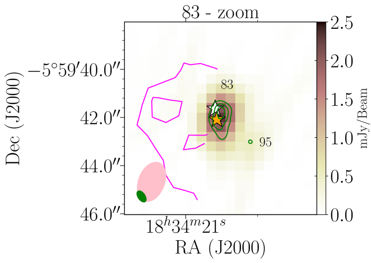
Figure 14: VLA C band (6 cm) continuum emission map of the radio jet candidates #83 and #95 located in the region IRAS 18316$-$1602. A close-up view of the two radio sources is shown in the bottom panel. The green contour levels of the K band (1.3 cm) continuum emission are 3, 5, 9 and 11 times 27 $\mu$Jy beam^-1. The magenta contours show the Spitzer/GLIMPSE 4.5 $\mu$m emission (note that half of the region was not covered in the mapped area). The blue- and red-shifted outflow lobed of SiO (2$-$1) are shown as blue-solid and red-dashed contours, respectively (see Sánchez-Monge et al. 2013d). The pink and green ellipses are the beam sizes of the C and K bands, respectively. The white and orange stars mark the location of the H₂O and CH₃OH masers, respectively (see Table 4).

G24.08$+$0.0 M2 (#96)

We have identified fourteen radio continuum sources in the region G24.08$+$0.0 M2, one of which, source #96, is detected in both frequency bands and has a negative spectral index ($-0.84\pm+0.08$, see Fig. 15). The outflow activity in the region has been studied by López-Sepulcre et al. (2011) and Sánchez-Monge et al. (2013d) who found molecular outflow in different tracers. However, this outflow is not spatially related to any of the radio continuum sources identified in this work. Also, this source could be a background source.

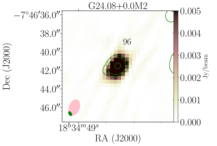
Figure 15: VLA C band (6 cm) continuum emission map of the radio source #96 located in the region G24.08$+$0.0M2. The green contour levels of the K band (1.3 cm) continuum emission are 3, 5 and 9 times 20 $\mu$Jy beam^-1. The pink and green ellipses are the beam sizes of the C and K bands, respectively.

G24.33$+$0.1 M1 (#110)

In the region G24.33$+$0.1 M1 we identified a radio continuum source (#110) located in the center of our field of view and detected in both frequency bands (see Fig. 16). This source has a positive spectral index of $+0.73\pm 0.35$, which is consistent with thermal emission. We have also detected maser features of both H₂O and CH₃OH associated with the continuum source. In addition, other authors have reported the presence of OH masers towards this object (see e.g., Caswell & Green 2011). Rathborne et al. (2007) studied this source in the millimeter regime, and identified a singular compact source with a rich chemistry characteristic of hot molecular cores. Sánchez-Monge et al. (2013d) reported molecular outflow activity, with the source #110 at its geometric center. Overall, this source is one of the best candidates for a thermal radio jet.

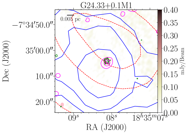
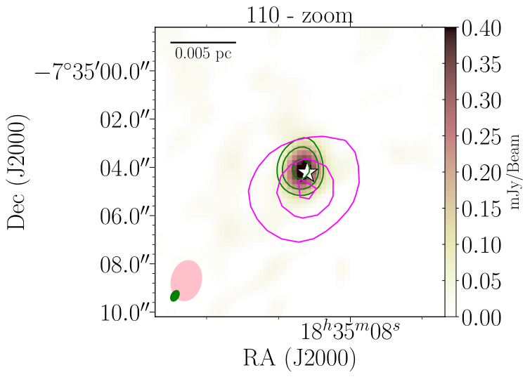
Figure 16: VLA C band (6 cm) continuum emission map of the radio jet candidate #110 located in the region G24.33+0.1 M1. A close-up view of the radio source is shown in the bottom panel. The green contour levels of the K band (1.3 cm) continuum emission are 3, 5 and 9 times 7 $\mu$Jy beam^-1. The blue- and red-shifted outflow lobed of SiO (2$-$1) are shown as blue-solid and red-dashed contours, respectively (see Sánchez-Monge et al. 2013d). The pink and green ellipses are the beam sizes of the C and K bands, respectively. The white star marks the location of the H₂O (see Table 4).

G24.60$+$0.1M1 (#119)

As for #119, the only information we have is that it is associated with an EGO. The nearest studied object is a extended H₂ emission that is 19^″ away from #119 (Froebrich et al. 2015). We can only say that we cannot determine the spectral index because the source is outside the primary beam of the K band images, but we propose that #119 is a radio jet.

G24.60$+$0.1M2 (#136)

Source #136 is detected only in the K band, resulting in a spectral index limit ($>+1.67$) that is consistent with thermal emission. The source is associated with H₂O maser emission. This source, although not directly associated with one EGO, is located in the vicinity of G24.63$+$0.15 reported by Cyganowski et al. (2008, see green circle in Fig. 17). Rathborne et al. (2007) suggest that the main dense condensation, hosting source #136, may contain several condensations, referred to as G024.60$+$00.08 MM1 (A, B, and C). Our radio continuum source appears to be related to component C which is an IRDC condensation. Further observations of this object are necessary to confirm its possible nature as a radio jet.

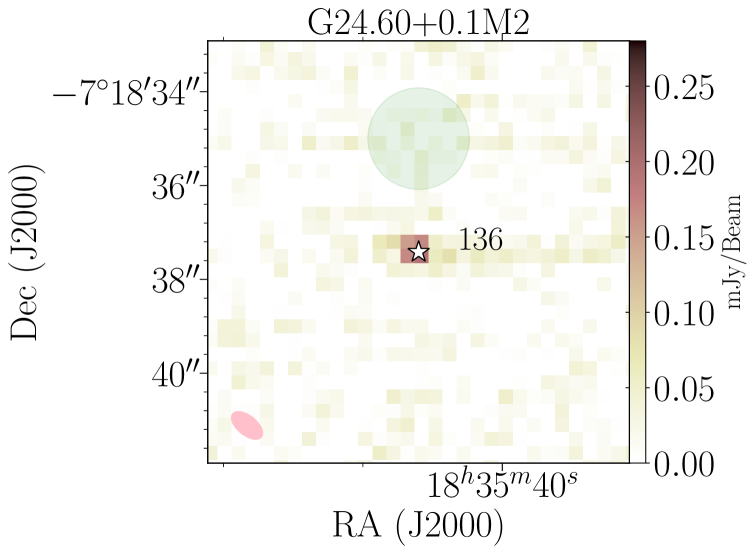
Figure 17: VLA K band (1.3 cm) continuum emission map of the radio jet candidate #136 located in the region G24.60$+$0.1 M2. The green circle with a radius of $\sim$4^″ marks EGO G24.63$+$0.15, reported by Cyganowski et al. (2008). The pink ellipse is the beam size of the K band. The white star marks the location of the H₂O (see Table 4).

G34.43$+$0.2M3 (#137 and #139)

Our radio continuum observations towards the region G34.43$+$0.2 M3 have led to the discovery of six radio continuum sources, although most of them are located far from the central region studied in Sánchez-Monge et al. (2013d). The brightest source is #137, which is about 13′ from the phase center of our observations, i.e., the source is outside the primary beam responses of the VLA antennas on both bands. This object is so bright that it is detected in both the C and K bands. At 6 cm, the source appears as a comet-like structure (see Fig. 18), which resembles cometary H ii regions. The 1.3 cm continuum emission also shows an arc-shaped structure shifted to the east, probably tracing the head of the cometary object. This source, referred to in the literature as G34.26$+$0.15, has been studied by other authors who report the presence of two hyper-compact H ii regions (A and B) and one ultra-compact H ii region (C), all marked in the Figure (see also Reid & Ho 1985; Gaume et al. 1994; Sewiło et al. 2011). Various studies (e.g., Hatchell et al. 2001; Liu et al. 2013) have reported the presence of outflow activity in this region, but no information on the outflow energetics such as the outflow momentum rate is reported. Despite this source is associated with an EGO (Cyganowski et al. 2008) and with a molecular outflow, the bright emission together with previous studies suggests that a major fraction of the radio continuum emission we have detected is originated in a H ii region rather than in a radio jet. Source #139 in the region, is also classified as a radio jet candidate in Table 3. However, the only information we have this object is its association with an EGO (i.e., G34.41$+$0.24, Cyganowski et al. 2008). Shepherd et al. (2004) suggest that the embedded object (G34.4 MM) appears to be a massive B2 protostar at an early stage of evolution. This region is also associated with the H₂O maser activity (Cyganowski et al. 2013), which may favor a radio jet origin for the detected radio continuum emission. Further observations are needed to better constrain its properties.

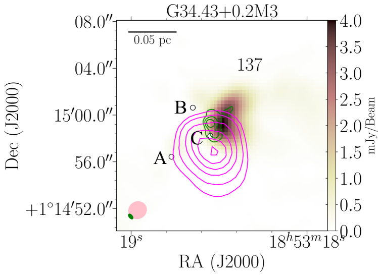
Figure 18: VLA C band (6 cm) continuum emission map of the radio jet candidate #137 located in the region G34.43$+$0.2 M3. The green contour levels of the K band (1.3 cm) continuum emission are 3, 5 and 7 times 20 $\mu$Jy beam^-1. The magenta contours show the Spitzer/GLIMPSE 4.5 $\mu$m emission. The pink and green ellipses are the beam sizes of the C and K bands, respectively. The white circles (A, B, and C) mark the position of 2 mm continuum sources reported by Gasiprong et al. (2002).

IRAS 19095$+$0930 (#143 and #144)

We have identified four radio continuum sources in the region IRAS 19095$+$0930, also known in the literature as G43.80$-$0.13). Two of these radio sources, #143 and #144, are located close to each other and in the center of a molecular outflow (Sánchez-Monge et al. 2013d, see also Figure 19). The source #143 has a brighter flux, is also clearly visible in the K band image, and is associated with H₂O maser emission features.

This region has been studied in the past by different authors at different wavelengths (Kurtz et al. 1994; Lekht 2000; De Buizer et al. 2005). De Buizer et al. (2005) report a kidney-bean shape structure at mid-infrared wavelengths that match the radio continuum sources reported by Kurtz et al. (1994) refers to as a H ii region. The object is also associated with OH masers. We have not found this source in the EGO catalogues (Cyganowski et al. 2008, 2009), but we have identified a 4.5 $\mu$m source associated with #143. No 4.5 $\mu$m infrared source appears to be associated with the eastern source #144.

We derive a spectral index of $+1.12\pm 0.04$ for #143, which is consistent with thermal emission. This, together with its location at the geometrical center of the outflow, and its association with masers may suggest that #143 is a good radio jet candidate. However, the large radio continuum flux of this source seem to not be consistent with the typical properties of other radio jets (see Figs. 3 and 5). This might mean that this source is in a transition phase from a radio jet to an H ii region. However, this requires further investigation.

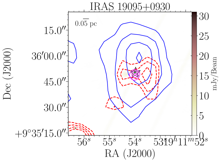
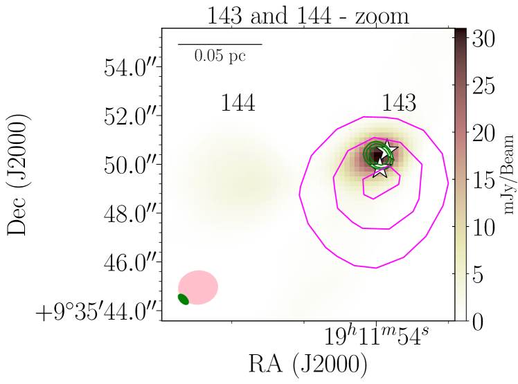
Figure 19: VLA C band (6 cm) continuum emission map of the radio sources #143 and #144 located in the region IRAS 19095$+$0930. The green contour levels of the K band (1.3 cm) continuum emission are 3, 5 and 9 times 2 mJy beam^-1. The blue- and red-shifted outflow lobed of SiO (2$-$1) are shown as blue-solid and red-dashed contours, respectively (see Sánchez-Monge et al. 2013d). The magenta contours show the Spitzer/GLIMPSE 4.5 $\mu$m emission. The pink and green ellipses are the beam sizes of the C and K bands, respectively. The white and orange stars mark the of the H₂O and CH₃OH masers (see Table 4).

Appendix B Catalog of the continuum sources

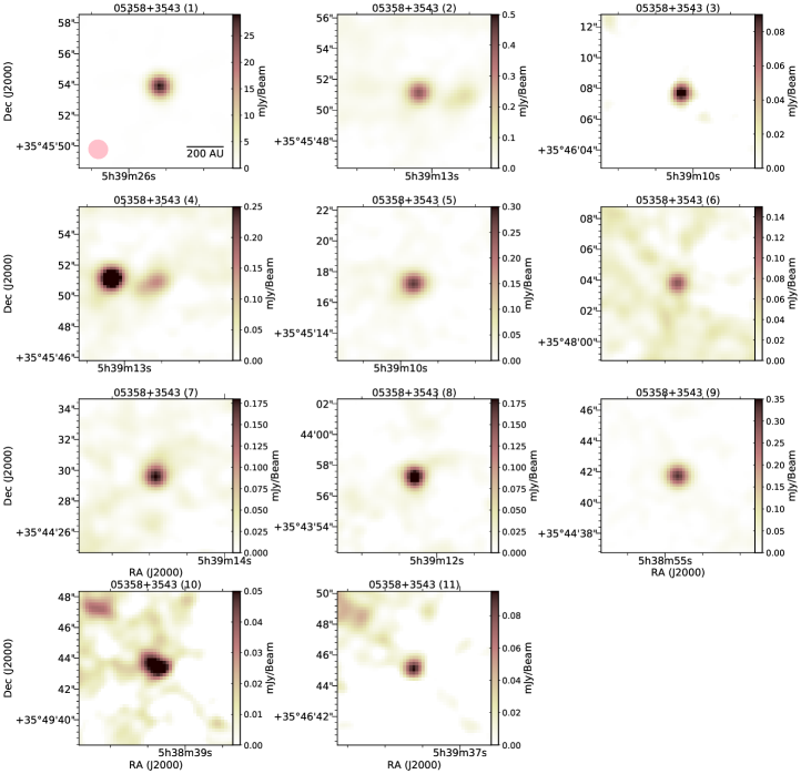
Figure 20: Close-up views of the C band (color scale image) and K band (contours) continuum images for the sources listed in Table LABEL:t:catalogue. Maps for the sources detected in region IRAS 05358$+$3543.

In the following tables and figures, we provide information on the properties of the radio continuum sources detected in the VLA observations presented in this work. In Table LABEL:t:catalogue, we list the coordinates of the 146 radio continuum sources together with their flux density, intensity peak and deconvolved size at 6 cm (C band) and 1.3 cm (K band). The fluxes and intensities are corrected by the primary beam response of the VLA antennas. For sources outside the C band primary beam (listed as ”oC” in column (11) of Table LABEL:t:catalogue) the primary beam correction is not reliable and the flux has to be taken with caution. Similarly, for sources located outside the K band primary beam (labelled as ”oK” in the Table), the K band flux has to be taken with caution. The last column of the Table lists the spectral index, $\alpha$. For sources with no reliable flux estimate at one of the bands, we do not determine the spectral index. For sources detected at both frequency bands (C and K bands), the spectral index has been determined using the fluxes determined after creating images with a common uv-range (see Sect. 3.2 for more details). In Table LABEL:t:sizes, we list the observed and deconvolved source sizes of all the detected sources. The source sizes are determined as $\sqrt{\theta_{\mathrm{major}}\times\theta_{\mathrm{minor}}}$, where $\theta_{\mathrm{major}}$ and $\theta_{\mathrm{minor}}$ are listed in Table LABEL:t:sizes. We transform the angular size of each source into astronomical unit (au) using the distances listed in Table 1. We give the source size in Table LABEL:t:catalogue. Finally, in Table 7, we list the intensities, flux densities and sizes determined from the images generated using a common uv-range at both C and K bands. In Figs. 20 to 35, we present close-up views of the C and K band emission for the 146 detected continuum sources.

Table 5: Catalogue of radio continuum sources detected with the VLA.

		Coordinates			C band				K band
		R.A.(J2000)	Dec.(J2000)		Intensity	Flux	Size		Intensity	Flux	Size		Spectral
ID	Region	(h:m:s)	(°:′:″)		(mJy beam-1)	(mJy)	(au)		(mJy beam-1)	(mJy)	(au)		index
1	IRAS 05358$+$3543	05:39:25.838	$+$35:45:53.861		37.733$\pm$0.272	038.134$\pm$0.272	¡2200		—	—	—	iC/oK	—
2		05:39:13.064	$+$35:45:51.125		00.387$\pm$0.010	000.534$\pm$0.014	¡1300		—	—	—	iC/iK	—
3		05:39:10.056	$+$35:46:07.731		00.105$\pm$0.003	000.075$\pm$0.002	¡1800		—	—	—	iC/iK	—
4		05:39:12.839	$+$35:45:50.854		00.147$\pm$0.006	000.332$\pm$0.015	¡2200		—	—	—	iC/iK	—
5		05:39:09.938	$+$35:45:17.196		00.267$\pm$0.008	000.403$\pm$0.013	¡1500		—	—	—	iC/iK	—
6		05:39:33.539	$+$35:48:03.740		00.282$\pm$0.006	000.345$\pm$0.007	¡1000		—	—	—	iC/oK	—
7		05:39:14.367	$+$35:44:29.634		00.191$\pm$0.006	000.266$\pm$0.009	¡1300		—	—	—	iC/iK	—
8		05:39:12.120	$+$35:44:02.155		00.238$\pm$0.006	000.262$\pm$0.007	0¡500		—	—	—	iC/iK	—
9		05:38:54.931	$+$35:44:41.720		00.521$\pm$0.004	000.571$\pm$0.005	0¡600		—	—	—	iC/oK	—
10		05:38:39.158	$+$35:49:43.533		00.886$\pm$0.060	001.640$\pm$0.110	¡2000		—	—	—	iC/oK	—
11		05:39:37.247	$+$35:46:45.155		00.265$\pm$0.014	000.197$\pm$0.010	¡1900		—	—	—	iC/oK	—
12	G189.78$+$0.34	06:08:35.111	$+$20:39:12.570		00.429$\pm$0.016	000.722$\pm$0.027	¡1700		—	—	—	iC/iK	—
13		06:08:35.273	$+$20:39:09.010		00.874$\pm$0.032	001.241$\pm$0.046	¡1300		—	—	—	iC/iK	—
14		06:08:35.308	$+$20:39:06.771		00.372$\pm$0.024	000.687$\pm$0.045	¡1900		—	—	—	iC/iK	—
15		06:08:35.380	$+$20:39:04.423		00.313$\pm$0.013	000.938$\pm$0.040	¡2800		—	—	—	iC/iK	—
16		06:08:35.449	$+$20:39:03.118		00.503$\pm$0.021	001.040$\pm$0.044	¡2000		—	—	—	iC/iK	—
17		06:08:43.600	$+$20:41:08.591		00.183$\pm$0.008	000.119$\pm$0.005	¡1700		—	—	—	iC/oK	—
18		06:08:45.199	$+$20:38:16.647		00.114$\pm$0.008	000.164$\pm$0.011	¡1300		—	—	—	iC/oK	—
19		06:08:36.598	$+$20:43:14.366		00.185$\pm$0.015	000.300$\pm$0.024	0¡800		—	—	—	iC/oK	—
20		06:08:44.256	$+$20:33:06.465		00.595$\pm$0.038	000.569$\pm$0.036	¡2000		—	—	—	iC/oK	—
21	G192.58$-$0.04	06:12:53.607	$+$18:00:26.360		12.029$\pm$0.460	018.208$\pm$0.701	¡2400		—	—	—	iC/iK	—
22		06:12:54.013	$+$17:59:23.202		03.998$\pm$0.087	010.274$\pm$0.220	¡4000		—	—	—	iC/iK	—
23		06:12:53.842	$+$17:59:22.168		01.540$\pm$0.047	001.558$\pm$0.047	¡3300		—	—	—	iC/iK	—
24		06:12:54.299	$+$17:59:33.802		00.637$\pm$0.033	000.494$\pm$0.025	¡2900		—	—	—	iC/iK	—
25		06:12:54.335	$+$17:59:24.274		00.303$\pm$0.011	000.470$\pm$0.049	¡5800		—	—	—	iC/iK	—
26		06:12:49.910	$+$18:03:05.366		00.313$\pm$0.009	000.408$\pm$0.012	¡1500		—	—	—	iC/oK	—
27	G18.18$-$0.30	18:25:01.066	$-$13:15:39.515		04.240$\pm$0.262	021.202$\pm$1.367	¡6600		…	…	…	iC/oK	…
28		18:25:07.460	$-$13:17:58.837		02.412$\pm$0.089	003.863$\pm$0.144	¡2200		…	…	…	iC/oK	…
29		18:25:06.979	$-$13:18:10.638		01.745$\pm$0.034	003.390$\pm$0.069	¡3000		…	…	…	iC/oK	…
30		18:25:01.186	$-$13:15:45.881		01.303$\pm$0.020	001.989$\pm$0.032	¡2400		…	…	…	iC/oK	…
31		18:25:00.956	$-$13:15:35.726		01.298$\pm$0.039	006.719$\pm$0.204	¡7000		…	…	…	iC/oK	…
32		18:24:44.852	$-$13:14:45.806		02.647$\pm$0.036	004.447$\pm$0.064	¡2400		…	…	…	iC/oK	…
33		18:24:53.825	$-$13:12:52.490		00.713$\pm$0.007	000.670$\pm$0.007	¡3400		…	…	…	iC/oK	…
34		18:25:06.706	$-$13:12:28.027		00.307$\pm$0.008	000.331$\pm$0.009	¡3600		…	…	…	iC/oK	…
35		18:25:42.356	$-$13:10:21.217		00.361$\pm$0.023	001.177$\pm$0.075	¡4500		…	…	…	oC	…
36		18:25:18.546	$-$13:15:33.062		00.182$\pm$0.006	000.259$\pm$0.009	¡2100		…	…	…	iC/oK	…
37		18:24:55.788	$-$13:10:16.391		00.404$\pm$0.023	001.782$\pm$0.101	¡6400		…	…	…	iC/oK	…
38		18:24:55.941	$-$13:10:17.447		00.291$\pm$0.012	001.226$\pm$0.053	¡6100		…	…	…	iC/oK	…
39	IRAS 18223$-$1243	18:25:31.473	$-$12:41:24.031		54.190$\pm$1.078	105.645$\pm$2.077	¡4500		…	…	…	iC/oK	…
40		18:25:04.143	$-$12:37:44.910		48.631$\pm$1.238	075.337$\pm$1.932	¡3800		…	…	…	iC/oK	…
41		18:25:26.731	$-$12:40:33.237		01.694$\pm$0.063	002.477$\pm$0.094	¡3600		…	…	…	iC/oK	…
42		18:24:52.605	$-$12:39:19.804		02.989$\pm$0.054	004.158$\pm$0.075	¡2900		…	…	…	iC/oK	…
43		18:24:36.306	$-$12:51:03.315		01.762$\pm$0.091	006.550$\pm$0.340	¡8800		…	…	…	oC	…
44		18:24:34.617	$-$12:52:03.911		00.374$\pm$0.016	001.583$\pm$0.069	¡9600		…	…	…	oC	…
45		18:26:04.962	$-$12:34:35.177		00.250$\pm$0.009	000.577$\pm$0.023	¡6000		…	…	…	oC	…
46		18:26:05.248	$-$12:34:35.621		00.289$\pm$0.039	000.579$\pm$0.039	¡8200		…	…	…	oC	…
47		18:24:34.692	$-$12:50:59.457		00.771$\pm$0.083	001.542$\pm$0.083	¡168000		…	…	…	oC	…
48a	IRAS 18228$-$1312	18:25:41.925	$-$13:10:17.630		21.200$\pm$0.450	219.960$\pm$5.101	¡135000		06.992$\pm$0.835	13.782$\pm$2.314	$<$7500	iC/iK	$-$2.11$\pm$0.13†
48b		18:25:42.059	$-$13:10:16.545		19.373$\pm$0.720	383.051$\pm$9.900	¡191000		06.218$\pm$1.203	14.341$\pm$3.711	¡5400	iC/iK	$-$2.51$\pm$0.20†
48c		18:25:42.407	$-$13:10:22.149		38.507$\pm$2.700	297.053$\pm$9.900	¡112000		25.098$\pm$1.807	64.552$\pm$6.425	¡6500	iC/iK	$-$1.17$\pm$0.10†
49		18:26:26.274	$-$13:05:48.537		00.468$\pm$0.010	000.445$\pm$0.009	¡4300		…	…	…	oC	…
50		18:25:00.730	$-$13:15:35.808		00.312$\pm$0.019	013.170$\pm$0.800	¡283000		…	…	…	oC	…
51	G19.27$+$0.1M1	18:27:37.962	$-$11:56:33.896		00.348$\pm$0.023	002.140$\pm$0.140	¡8200		…	…	…	oC	…
52		18:26:20.973	$-$12:05:33.129		00.797$\pm$0.033	000.878$\pm$0.037	¡1100		…	…	…	iC/oK	…
53		18:26:03.677	$-$12:04:37.085		01.130$\pm$0.019	001.198$\pm$0.020	0¡800		…	…	…	iC/iK	$<-$0.57
54		18:25:45.520	$-$12:05:18.590		00.265$\pm$0.005	000.326$\pm$0.007	¡1400		…	…	…	iC/oK	…
55		18:25:54.272	$-$11:52:19.022		00.186$\pm$0.012	001.138$\pm$0.071	¡3600		…	…	…	oC	…
56		18:26:04.228	$-$11:52:32.053		00.299$\pm$0.041	007.300$\pm$1.000	¡176000		…	…	…	oC	…
57		18:26:48.638	$-$12:26:17.050		00.199$\pm$0.009	000.599$\pm$0.030	¡5000		…	…	…	oC	…
58		18:26:34.300	$-$11:57:59.910		00.284$\pm$0.008	000.518$\pm$0.016	¡3100		…	…	…	oC	…
59		18:26:13.780	$-$12:01:19.596		00.258$\pm$0.007	000.249$\pm$0.006	¡3500		…	…	…	iC/oK	…
60		18:27:37.166	$-$11:56:26.273		00.168$\pm$0.008	000.409$\pm$0.021	¡2200		…	…	…	oC	…
61		18:26:05.577	$-$12:04:33.534		00.123$\pm$0.003	000.139$\pm$0.003	¡4300		…	…	…	iC/iK	$<+$2.07
62		18:25:51.964	$-$12:05:13.440		…	…	…		00.203$\pm$0.006	000.244$\pm$0.092	$<$1100	iC/iK	$>+$1.23
63	IRAS 18236$-$1205	18:26:25.064	$-$12:03:48.923		00.070$\pm$0.004	000.099$\pm$0.006	¡1100		00.281$\pm$0.010	000.140$\pm$0.010	¡2800	iC/iK	$+$0.26$\pm$0.21†
64		18:26:25.782	$-$12:03:53.203		00.331$\pm$0.013	000.383$\pm$0.015	¡4300		00.182$\pm$0.006	000.280$\pm$0.010	¡0930	iC/iK	$-$0.24$\pm$0.12†
65		18:26:26.380	$-$12:04:19.782		00.558$\pm$0.004	000.570$\pm$0.004	¡4000		01.774$\pm$0.004	001.960$\pm$0.006	¡0310	iC/iK	$+$0.94$\pm$0.02†
66		18:26:35.471	$-$12:01:13.807		00.125$\pm$0.002	000.113$\pm$0.002	¡3800		…	…	…	iC/oK	…
67		18:26:22.554	$-$12:05:58.888		00.224$\pm$0.035	000.708$\pm$0.060	¡7400		…	…	…	iC/oK	…
68		18:26:22.308	$-$12:05:58.065		00.135$\pm$0.005	000.270$\pm$0.020	¡6000		…	…	…	iC/oK	…
69		18:26:22.051	$-$12:07:28.996		00.092$\pm$0.003	000.449$\pm$0.034	¡9700		…	…	…	iC/oK	…
70		18:26:21.849	$-$12:07:31.842		00.070$\pm$0.001	000.143$\pm$0.019	¡4300		…	…	…	iC/oK	…
71		18:26:21:659	$-$12:07:35.409		00.198$\pm$0.001	000.394$\pm$0.031	¡6500		…	…	…	iC/oK	…
72	G23.60$+$0.0M1	18:33:53.474	$-$08:07:12.198		00.817$\pm$0.110	009.900$\pm$1.300	¡119000		…	…	…	oC	…
73		18:34:12.339	$-$08:19:01.195		00.191$\pm$0.003	000.190$\pm$0.003	¡3600		00.357$\pm$0.042	000.480$\pm$0.054	$<$1200	iC/iK	$+$0.70$\pm$0.26†
74		18:34:11.574	$-$08:19:06.420		00.310$\pm$0.004	000.328$\pm$0.004	¡3700		00.109$\pm$0.045	001.040$\pm$0.430	¡1100	iC/iK	$+$0.87$\pm$0.94†
75		18:34:21.063	$-$08:18:12.357		00.420$\pm$0.006	000.452$\pm$0.006	0¡800		…	…	…	iC/oK	…
76		18:34:33.022	$-$08:15:26.757		11.325$\pm$0.194	012.813$\pm$0.219	¡1200		…	…	…	iC/oK	…
77		18:34:44.839	$-$08:31:05.331		00.210$\pm$0.003	000.272$\pm$0.003	¡1700		…	…	…	oC	…
78		18:33:44.014	$-$08:21:22.952		01.234$\pm$0.038	002.500$\pm$0.077	¡3500		…	…	…	iC/oK	…
79		18:33:47.803	$-$08:23:34.272		00.763$\pm$0.049	001.718$\pm$0.109	¡3900		…	…	…	iC/oK	…
80		18:34:06.126	$-$08:24:38.779		00.276$\pm$0.012	000.336$\pm$0.015	¡3900		…	…	…	iC/oK	…
81		18:34:17.741	$-$08:21:08.236		00.096$\pm$0.004	000.119$\pm$0.005	¡4000		…	…	…	iC/oK	…
82		18:34:14.297	$-$08:24:10.308		00.351$\pm$0.010	000.390$\pm$0.011	¡3800		…	…	…	iC/oK	…
83	IRAS 18316$-$0602	18:34:20.904	$-$05:59:41.968		02.275$\pm$0.081	003.345$\pm$0.120	¡2500		00.606$\pm$0.062	002.621$\pm$0.259	¡2000	iC/iK	$-$0.19$\pm$0.24†
84		18:34:33.930	$-$06:02:21.993		01.618$\pm$0.025	001.863$\pm$0.029	¡1200		…	…	…	iC/oK	…
85		18:34:27.632	$-$06:05:09.136		02.103$\pm$0.026	002.493$\pm$0.030	¡1300		…	…	…	iC/oK	…
86		18:34:14.921	$-$06:00:23.582		00.313$\pm$0.005	000.354$\pm$0.006	¡4400		…	…	…	iC/iK	$<+$1.43
87		18:34:26.746	$-$05:57:21.183		00.907$\pm$0.016	000.998$\pm$0.019	¡4400		…	…	…	iC/oK	…
88		18:34:16.533	$-$05:45:48.502		00.109$\pm$0.006	000.742$\pm$0.045	¡9900		…	…	…	oC	…
89		18:32:42.034	$-$06:10:19.838		00.146$\pm$0.011	000.301$\pm$0.022	¡3700		…	…	…	oC	…
90		18:34:08.906	$-$05:52:55.202		01.454$\pm$0.064	001.658$\pm$0.073	¡4500		…	…	…	iC/oK	…
91		18:34:32.327	$-$06:00:15.075		00.130$\pm$0.007	000.147$\pm$0.008	¡4400		…	…	…	iC/oK	…
92		18:34:13.821	$-$05:53:01.189		00.405$\pm$0.013	000.971$\pm$0.031	¡3400		…	…	…	iC/oK	…
93		18:35:10.900	$-$06:02:32.533		00.067$\pm$0.001	000.136$\pm$0.008	¡4000		…	…	…	oC	…
94		18:34:17.698	$-$06:05:05.398		…	…	…		00.222$\pm$0.006	000.311$\pm$0.009	¡2100	iC/oK	…
95		18:34:20.819	$-$05:59:42.997		…	…	…		00.227$\pm$0.037	000.251$\pm$0.069	$<$1300	iC/iK	$>+$1.36
96	G24.08$+$0.0M2	18:34:48.710	$-$07:46:41.510		16.982$\pm$0.338	021.761$\pm$0.433	¡1600		04.098$\pm$0.166	005.300$\pm$0.212	$<$1100	iC/iK	$-$1.08$\pm$0.10†
97		18:34:41.391	$-$07:43:55.450		07.986$\pm$0.172	010.670$\pm$0.239	¡1600		…	…	…	iC/oK	…
98		18:34:41.452	$-$07:43:47.693		01.411$\pm$0.017	002.558$\pm$0.032	¡3000		…	…	…	iC/oK	…
99		18:34:57.182	$-$07:43:26.184		03.122$\pm$0.052	004.364$\pm$0.073	¡2000		…	…	…	iC/oK	…
100		18:34:59.593	$-$07:43:00.526		03.762$\pm$0.104	007.750$\pm$0.217	¡3500		…	…	…	iC/oK	…
101		18:34:59.600	$-$07:42:57.062		01.208$\pm$0.021	002.517$\pm$0.089	¡2800		…	…	…	iC/oK	…
102		18:34:57.132	$-$07:45:22.485		01.141$\pm$0.014	001.454$\pm$0.017	¡1700		…	…	…	iC/iK	$<-$0.06
103		18:34:12.138	$-$07:52:54.065		00.136$\pm$0.004	000.202$\pm$0.005	¡2400		…	…	…	oC	…
104		18:34:11.271	$-$07:53:07.879		00.088$\pm$0.004	000.146$\pm$0.006	¡2800		…	…	…	oC	…
105		18:33:59.500	$-$07:52:36.635		00.304$\pm$0.005	000.608$\pm$0.056	¡7600		…	…	…	oC	…
106		18:34:25.403	$-$07:54:46.135		00.239$\pm$0.074	059.000$\pm$18.00	¡557000		…	…	…	oC	…
107		18:34:51.288	$-$07:42:14.421		00.094$\pm$0.005	000.195$\pm$0.033	¡2900		…	…	…	iC/oK	…
108		18:35:23.922	$-$07:37:38.200		01.510$\pm$0.150	002.080$\pm$0.020	¡3500		…	…	…	oC	…
109		18:34:52.966	$-$07:47:03.052		00.041$\pm$0.003	000.082$\pm$0.032	¡2300		…	…	…	iC/iK	$<+$2.33
110	G24.33$+$0.1M1	18:35:08.132	$-$07:35:04.176		00.438$\pm$0.007	000.434$\pm$0.007	¡5400		00.769$\pm$0.029	000.905$\pm$0.034	$<$1600	iC/iK	$+$0.55$\pm$0.09†
111		18:35:13.569	$-$07:38:20.379		00.382$\pm$0.014	000.659$\pm$0.024	¡2700		…	…	…	iC/oK	…
112		18:35:33.971	$-$07:37:34.491		01.630$\pm$0.078	004.685$\pm$0.228	¡7400		…	…	…	iC/oK	…
113		18:35:10.888	$-$07:34:22.080		00.198$\pm$0.007	000.278$\pm$0.011	¡3200		…	…	…	iC/iK	$<+$0.07
114		18:35:02.821	$-$07:31:20.729		00.290$\pm$0.005	000.328$\pm$0.005	¡2000		…	…	…	iC/oK	…
115		18:34:48.656	$-$07:46:40.369		00.151$\pm$0.006	000.225$\pm$0.009	¡3700		…	…	…	oC	…
116		18:35:56.006	$-$07:27:23.278		00.196$\pm$0.009	000.289$\pm$0.015	¡2400		…	…	…	oC	…
117	G24.60$+$0.1M1	18:36:12.517	$-$07:12:09.922		00.437$\pm$0.015	000.526$\pm$0.018	¡1300		…	…	…	oC	…
118		18:36:12.607	$-$07:12:14.144		00.420$\pm$0.022	000.983$\pm$0.052	¡5700		…	…	…	oC	…
119		18:35:40.677	$-$07:22:05.797		00.305$\pm$0.016	001.107$\pm$0.059	¡8400		…	…	…	iC/oK	…
120		18:35:40.739	$-$07:22:00.863		00.284$\pm$0.009	000.457$\pm$0.014	¡3000		…	…	…	iC/oK	…
121		18:35:40.869	$-$07:21:57.887		00.286$\pm$0.020	001.705$\pm$0.126	¡109000		…	…	…	iC/oK	…
122		18:36:05.589	$-$07:31:21.640		00.349$\pm$0.036	003.790$\pm$0.390	¡162000		…	…	…	oC	…
123		18:35:53.123	$-$07:14:20.492		01.058$\pm$0.011	001.164$\pm$0.012	¡5500		…	…	…	iC/oK	…
124		18:35:16.807	$-$07:05:08.357		00.239$\pm$0.011	000.400$\pm$0.019	¡3800		…	…	…	oC	…
125		18:35:41.070	$-$07:16:41.062		00.140$\pm$0.004	000.123$\pm$0.004	¡4900		…	…	…	iC/iK	…
126		18:35:43.769	$-$07:19:26.186		00.114$\pm$0.003	000.105$\pm$0.002	¡5000		…	…	…	iC/iK	$<+$0.96
127		18:35:03.755	$-$07:26:00.913		00.146$\pm$0.012	000.529$\pm$0.044	¡8400		…	…	…	oC	…
128		18:36:18.116	$-$07:08:50.104		00.128$\pm$0.003	000.705$\pm$0.018	¡110000		…	…	…	oC	…
129		18:35:40.400	$-$07:19:28.740		00.088$\pm$0.005	000.157$\pm$0.009	¡4500		…	…	…	iC/iK	$<+$0.18
130		18:34:59.859	$-$07:26:39.367		00.078$\pm$0.002	000.110$\pm$0.003	¡3000		…	…	…	oC	…
131		18:34:39.433	$-$07:02:39.152		00.068$\pm$0.002	000.081$\pm$0.003	¡5700		…	…	…	oC	…
132	G24.60$+$0.1M2	18:35:47.199	$-$07:12:59.443		00.300$\pm$0.008	000.543$\pm$0.015	¡3800		…	…	…	iC/oK	…
133		18:35:40.955	$-$07:21:56.177		00.275$\pm$0.010	000.992$\pm$0.036	¡7600		…	…	…	iC/oK	…
134		18:35:56.070	$-$07:27:23.872		00.133$\pm$0.015	000.243$\pm$0.028	¡6500		…	…	…	oC	…
135		18:35:29.951	$-$07:27:46.840		00.064$\pm$0.003	000.077$\pm$0.003	¡1900		…	…	…	oC	…
136		18:35:40.124	$-$07:18:37.396		…	…	…		00.821$\pm$0.110	000.853$\pm$0.116	$<$2100	iC/iK	$>+$1.67
137	G34.43$+$0.2M3	18:53:18.845	$+$01:14:59.320		04.070$\pm$0.280	018.400$\pm$1.300	¡7000		00.242$\pm$0.022	001.270$\pm$0.120	¡2000	oC	…
138		18:53:18.672	$+$01:24:47.737		06.046$\pm$0.080	007.393$\pm$0.097	¡1600		…	…	…	iC/oK	…
139		18:53:18.020	$+$01:25:25.608		00.439$\pm$0.017	000.729$\pm$0.029	¡2100		…	…	…	iC/oK	…
140		18:53:08.320	$+$01:29:33.994		00.858$\pm$0.013	000.820$\pm$0.012	¡3000		…	…	…	iC/oK	…
141		18:53:35.990	$+$01:35:18.770		02.290$\pm$0.147	010.435$\pm$0.672	¡5600		…	…	…	iC/oK	…
142		18:54:14.014	$+$01:19:18.429		00.089$\pm$0.003	000.148$\pm$0.005	¡7100		…	…	…	oC	…
143	IRAS 19095$+$0930	19:11:53.997	$+$09:35:50.404		30.580$\pm$0.860	040.400$\pm$1.100	¡1900		90.545$\pm$2.101	126.364$\pm$3.001	¡0660	iC/iK	$+$0.87$\pm$0.08†
144		19:11:54.369	$+$09:35:49.254		04.211$\pm$0.240	015.565$\pm$0.890	¡7300		…	…	…	iC/iK	$<-$2.97
145		19:12:00.546	$+$09:36:24.232		02.847$\pm$0.023	002.838$\pm$0.023	¡4400		…	…	…	iC/iK	$<+$0.32
146		19:11:46.436	$+$09:37:03.679		01.927$\pm$0.025	002.048$\pm$0.027	¡4500		…	…	…	iC/oK	…

Table 5: continued.

Table 6: Observed and deconvolved angular sizes for the radio continuum sources detected in this work (see Table LABEL:t:catalogue)

		Observed source size				Deconvolved diameter
		Major axis	Minor axis	PA		Major axis	Minor axis	PA
ID	Region	(″)	(″)	(°)		(″)	(″)	(°)
Observed and deconvolved source sizes for C band detections
1	IRAS 05358$+$3543	01.269$\pm$0.009	01.239$\pm$0.009	053.0$\pm$3.8		…	…	…
2		01.532$\pm$0.034	01.402$\pm$0.034	106.7$\pm$3.4		00.894$\pm$0.063	00.633$\pm$0.085	114.9$\pm$9.9
3		01.113$\pm$0.044	01.001$\pm$0.043	155.4$\pm$5.2		…	…	…
4		02.411$\pm$0.058	01.455$\pm$0.057	120.4$\pm$1.1		02.069$\pm$0.069	00.730$\pm$0.124	121.1$\pm$1.2
5		01.667$\pm$0.041	01.409$\pm$0.041	104.5$\pm$2.0		01.105$\pm$0.065	00.654$\pm$0.098	108.5$\pm$3.8
6		01.412$\pm$0.028	01.349$\pm$0.027	000.1$\pm$7.5		00.690$\pm$0.066	00.472$\pm$0.094	169.0$\pm$9.0
7		01.520$\pm$0.046	01.424$\pm$0.044	145.4$\pm$6.4		00.899$\pm$0.082	00.644$\pm$0.106	147.1$\pm$6.4
8		01.330$\pm$0.035	01.286$\pm$0.034	168.0$\pm$9.0		00.512$\pm$0.758	00.215$\pm$1.011	160.0$\pm$9.0
9		01.357$\pm$0.012	01.255$\pm$0.012	076.4$\pm$1.4		00.490$\pm$0.035	00.249$\pm$0.076	085.0$\pm$9.0
10		01.918$\pm$0.083	01.502$\pm$0.086	065.3$\pm$3.1		01.440$\pm$0.110	00.870$\pm$0.160	065.6$\pm$3.8
11		01.089$\pm$0.070	01.065$\pm$0.068	135.0$\pm$9.0		…	…	…
12	G189.78$+$0.34	01.673$\pm$0.041	01.397$\pm$0.048	012.0$\pm$2.2		01.095$\pm$0.070	00.860$\pm$0.089	000.5$\pm$9.6
13		01.578$\pm$0.041	01.249$\pm$0.048	014.6$\pm$1.8		00.934$\pm$0.074	00.602$\pm$0.115	006.7$\pm$9.5
14		01.781$\pm$0.072	01.441$\pm$0.083	010.1$\pm$3.9		01.250$\pm$0.110	00.930$\pm$0.150	001.7$\pm$9.4
15		02.461$\pm$0.073	01.688$\pm$0.050	158.3$\pm$2.0		02.161$\pm$0.088	01.194$\pm$0.079	154.2$\pm$2.7
16		01.920$\pm$0.050	01.493$\pm$0.050	156.9$\pm$1.8		01.525$\pm$0.068	00.880$\pm$0.096	148.3$\pm$3.9
17		01.014$\pm$0.052	00.892$\pm$0.061	018.6$\pm$6.4		…	…	…
18		01.598$\pm$0.078	01.254$\pm$0.092	021.7$\pm$4.9		00.958$\pm$0.136	00.629$\pm$0.226	020.0$\pm$9.0
19		01.959$\pm$0.091	01.148$\pm$0.100	174.7$\pm$2.0		01.524$\pm$0.091	00.136$\pm$0.100	169.9$\pm$2.0
20		01.382$\pm$0.071	00.961$\pm$0.083	016.5$\pm$2.4		…	…	…
21	G192.58$-$0.04	01.741$\pm$0.046	01.451$\pm$0.054	025.8$\pm$2.2		01.033$\pm$0.082	00.827$\pm$0.106	032.0$\pm$9.0
22		02.524$\pm$0.064	01.700$\pm$0.029	059.1$\pm$1.5		02.152$\pm$0.078	01.116$\pm$0.052	063.7$\pm$2.1
23		01.454$\pm$0.036	01.162$\pm$0.043	030.3$\pm$1.8		…	…	…
24		01.206$\pm$0.066	01.073$\pm$0.072	170.4$\pm$6.4		…	…	…
25		02.903$\pm$0.050	02.375$\pm$0.038	148.1$\pm$2.4		02.614$\pm$0.060	01.961$\pm$0.052	143.0$\pm$3.1
26		01.745$\pm$0.050	01.247$\pm$0.042	028.1$\pm$1.9		01.043$\pm$0.064	00.360$\pm$0.221	032.0$\pm$4.4
27	G18.18$-$0.30	03.480$\pm$0.102	02.620$\pm$0.077	047.0$\pm$1.4		03.270$\pm$0.110	02.030$\pm$0.110	053.9$\pm$2.4
28		01.884$\pm$0.040	01.550$\pm$0.064	174.8$\pm$2.4		01.180$\pm$0.098	00.657$\pm$0.172	061.0$\pm$9.0
29		02.210$\pm$0.025	01.604$\pm$0.033	011.5$\pm$0.8		01.629$\pm$0.042	00.820$\pm$0.085	037.9$\pm$3.1
30		01.962$\pm$0.017	01.419$\pm$0.028	165.8$\pm$0.8		00.971$\pm$0.050	00.890$\pm$0.053	050.0$\pm$9.0
31		03.244$\pm$0.057	02.909$\pm$0.052	151.8$\pm$4.5		02.803$\pm$0.090	02.645$\pm$0.091	117.0$\pm$9.0
32		01.926$\pm$0.016	01.591$\pm$0.024	179.5$\pm$0.7		01.267$\pm$0.034	00.711$\pm$0.058	057.4$\pm$3.7
33		01.637$\pm$0.011	01.047$\pm$0.019	166.6$\pm$0.3		…	…	…
34		01.714$\pm$0.030	01.148$\pm$0.049	161.5$\pm$1.0		…	…	…
35		02.876$\pm$0.108	02.066$\pm$0.072	056.7$\pm$1.5		02.660$\pm$0.120	01.160$\pm$0.140	062.3$\pm$2.0
36		02.114$\pm$0.037	01.225$\pm$0.061	157.9$\pm$1.0		01.224$\pm$0.073	00.584$\pm$0.164	147.5$\pm$6.1
37		03.407$\pm$0.061	02.362$\pm$0.099	156.2$\pm$1.4		02.938$\pm$0.074	02.105$\pm$0.117	152.7$\pm$3.1
38		03.376$\pm$0.103	02.275$\pm$0.068	132.8$\pm$1.9		03.000$\pm$0.130	01.850$\pm$0.110	123.8$\pm$3.9
39	IRAS 18223$-$1243	02.267$\pm$0.027	01.865$\pm$0.034	018.1$\pm$0.8		01.715$\pm$0.043	00.882$\pm$0.088	054.0$\pm$3.4
40		02.167$\pm$0.030	01.550$\pm$0.048	172.3$\pm$0.7		01.163$\pm$0.073	00.920$\pm$0.096	033.0$\pm$9.0
41		02.230$\pm$0.044	01.423$\pm$0.072	166.4$\pm$1.0		01.178$\pm$0.085	00.844$\pm$0.132	168.0$\pm$9.0
42		02.064$\pm$0.021	01.461$\pm$0.034	175.2$\pm$0.5		01.053$\pm$0.055	00.622$\pm$0.099	041.7$\pm$7.7
43		03.002$\pm$0.060	02.684$\pm$0.098	161.3$\pm$2.7		02.440$\pm$0.120	02.320$\pm$0.100	091.0$\pm$9.0
44		03.271$\pm$0.056	02.803$\pm$0.078	142.1$\pm$1.7		02.810$\pm$0.081	02.401$\pm$0.104	116.0$\pm$9.0
45		02.538$\pm$0.046	01.970$\pm$0.075	158.5$\pm$1.5		01.748$\pm$0.088	01.538$\pm$0.113	129.0$\pm$9.0
46		02.548$\pm$1.973	01.973$\pm$0.091	157.0$\pm$7.0		…	…	…
47		05.050$\pm$0.250	04.120$\pm$0.200	143.0$\pm$9.0		…	…	…
48a	IRAS 18228$-$1312	06.450$\pm$0.144	03.501$\pm$0.070	004.3$\pm$1.2		06.189$\pm$0.153	03.268$\pm$0.080	005.7$\pm$1.5
48b		07.250$\pm$0.270	05.940$\pm$0.220	046.1$\pm$7.4		07.120$\pm$0.290	05.670$\pm$0.250	049.0$\pm$8.0
48c		04.610$\pm$0.340	03.640$\pm$0.250	065.0$\pm$9.0		04.450$\pm$0.370	03.130$\pm$0.320	067.0$\pm$9.0
49		01.784$\pm$0.025	01.160$\pm$0.040	163.8$\pm$0.7		…	…	…
50		11.100$\pm$0.080	08.271$\pm$0.107	140.4$\pm$0.5		10.960$\pm$0.082	08.164$\pm$0.109	139.5$\pm$0.6
51	G19.27$+$0.1M1	04.790$\pm$0.110	02.980$\pm$0.130	167.3$\pm$1.7		04.380$\pm$0.120	02.730$\pm$0.150	167.9$\pm$2.2
52		02.071$\pm$0.050	01.231$\pm$0.082	163.8$\pm$1.7		00.694$\pm$1.257	00.317$\pm$0.872	161.0$\pm$9.0
53		02.018$\pm$0.021	01.218$\pm$0.034	164.9$\pm$0.7		00.518$\pm$1.433	00.258$\pm$0.931	173.0$\pm$9.0
54		02.060$\pm$0.028	01.387$\pm$0.042	171.9$\pm$1.3		00.889$\pm$1.063	00.391$\pm$0.797	036.0$\pm$9.0
55		04.480$\pm$0.140	03.170$\pm$0.110	095.3$\pm$2.9		04.290$\pm$0.150	00.550$\pm$0.150	091.0$\pm$9.0
56		08.700$\pm$0.260	06.540$\pm$0.260	100.9$\pm$4.2		08.590$\pm$0.280	06.280$\pm$0.280	099.3$\pm$4.4
57		03.057$\pm$0.094	02.282$\pm$0.092	141.4$\pm$3.5		02.480$\pm$0.140	01.780$\pm$0.170	124.0$\pm$9.0
58		02.447$\pm$0.037	01.724$\pm$0.059	175.3$\pm$1.3		01.571$\pm$0.077	01.125$\pm$0.116	019.6$\pm$9.9
59		01.951$\pm$0.033	01.147$\pm$0.053	159.8$\pm$1.2		…	…	…
60		02.300$\pm$0.140	01.430$\pm$0.120	170.1$\pm$3.6		01.250$\pm$0.310	00.730$\pm$0.480	004.2$\pm$9.8
61		02.950$\pm$0.100	01.900$\pm$0.100	152.8$\pm$2.5		02.250$\pm$0.150	01.430$\pm$0.170	143.8$\pm$8.4
63	IRAS 18236$-$1205	00.485$\pm$0.019	00.393$\pm$0.021	134.6$\pm$7.2		…	…	…
64		02.229$\pm$0.061	01.148$\pm$0.079	170.1$\pm$1.5		…	…	…
65		02.033$\pm$0.012	01.112$\pm$0.017	163.6$\pm$0.3		…	…	…
66		01.785$\pm$0.044	01.121$\pm$0.042	156.1$\pm$1.6		…	…	…
67		04.068$\pm$1.886	01.886$\pm$0.093	116.0$\pm$2.0		…	…	…
68		02.633$\pm$0.156	01.893$\pm$0.092	138.0$\pm$6.0		…	…	…
69		06.040$\pm$0.820	02.180$\pm$0.210	003.0$\pm$3.0		…	…	…
70		01.840$\pm$0.170	01.400$\pm$0.100	126.0$\pm$9.0		…	…	…
71		03.193$\pm$0.223	01.823$\pm$0.093	159.0$\pm$4.0		…	…	…
72	G23.60$+$0.0M1	05.110$\pm$0.210	04.960$\pm$0.210	114.0$\pm$9.0		04.930$\pm$0.290	04.660$\pm$0.300	086.0$\pm$9.0
73		01.770$\pm$0.029	01.175$\pm$0.035	160.1$\pm$1.4		…	…	…
74		01.793$\pm$0.021	01.236$\pm$0.025	160.3$\pm$1.0		…	…	…
75		01.884$\pm$0.020	01.198$\pm$0.026	156.3$\pm$0.8		00.444$\pm$1.410	00.290$\pm$0.842	105.0$\pm$9.0
76		01.926$\pm$0.019	01.230$\pm$0.032	157.3$\pm$0.8		00.541$\pm$0.083	00.475$\pm$0.117	141.0$\pm$9.0
77		01.975$\pm$0.017	01.372$\pm$0.027	162.3$\pm$0.9		00.847$\pm$0.061	00.602$\pm$0.087	035.0$\pm$9.0
78		02.285$\pm$0.041	01.856$\pm$0.057	152.2$\pm$3.1		01.497$\pm$0.095	01.312$\pm$0.111	088.0$\pm$9.0
79		02.672$\pm$0.090	01.760$\pm$0.116	174.9$\pm$2.6		02.010$\pm$0.140	01.220$\pm$0.220	008.9$\pm$9.8
80		01.817$\pm$0.065	01.405$\pm$0.084	173.7$\pm$4.9		…	…	…
81		01.828$\pm$0.051	01.418$\pm$0.080	169.0$\pm$4.0		…	…	…
82		01.762$\pm$0.033	01.324$\pm$0.054	152.6$\pm$2.3		…	…	…
83	IRAS 18316$-$0602	01.987$\pm$0.041	01.376$\pm$0.060	174.1$\pm$1.9		01.181$\pm$0.096	00.592$\pm$0.228	022.5$\pm$9.8
84		01.741$\pm$0.018	01.230$\pm$0.028	163.2$\pm$1.1		00.620$\pm$1.085	00.251$\pm$0.838	046.0$\pm$9.0
85		01.759$\pm$0.014	01.253$\pm$0.021	165.1$\pm$0.9		00.696$\pm$0.053	00.283$\pm$0.184	041.5$\pm$7.6
86		01.683$\pm$0.021	01.250$\pm$0.031	163.2$\pm$1.7		…	…	…
87		01.685$\pm$0.021	01.215$\pm$0.032	159.8$\pm$1.4		…	…	…
88		04.688$\pm$0.090	02.687$\pm$0.094	013.0$\pm$1.1		04.434$\pm$0.099	02.333$\pm$0.117	016.2$\pm$1.5
89		02.250$\pm$0.100	01.690$\pm$0.110	118.4$\pm$4.7		01.790$\pm$0.160	00.800$\pm$0.400	098.0$\pm$9.0
90		01.709$\pm$0.050	01.240$\pm$0.074	145.2$\pm$3.2		…	…	…
91		01.521$\pm$0.081	01.376$\pm$0.099	172.0$\pm$9.0		…	…	…
92		02.140$\pm$0.110	01.500$\pm$0.110	145.9$\pm$4.7		01.380$\pm$0.230	00.910$\pm$0.330	124.0$\pm$9.0
93		02.474$\pm$0.119	01.509$\pm$0.075	173.9$\pm$2.4		01.840$\pm$0.180	00.950$\pm$0.170	004.0$\pm$7.9
96	G24.08$+$0.0M2	01.977$\pm$0.023	01.317$\pm$0.036	150.6$\pm$1.0		00.942$\pm$0.068	00.487$\pm$0.151	118.6$\pm$8.7
97		01.935$\pm$0.026	01.402$\pm$0.039	171.8$\pm$1.5		01.008$\pm$0.078	00.418$\pm$0.265	037.1$\pm$7.8
98		02.469$\pm$0.022	01.492$\pm$0.022	174.4$\pm$0.6		01.759$\pm$0.035	00.842$\pm$0.052	006.8$\pm$1.8
99		01.940$\pm$0.019	01.464$\pm$0.030	161.5$\pm$1.2		00.942$\pm$0.054	00.708$\pm$0.068	059.0$\pm$9.0
100		02.967$\pm$0.039	01.410$\pm$0.050	159.1$\pm$0.7		02.357$\pm$0.050	00.846$\pm$0.086	159.1$\pm$1.0
101		02.471$\pm$0.101	01.714$\pm$0.054	022.8$\pm$3.0		02.020$\pm$0.140	00.660$\pm$0.280	039.1$\pm$5.2
102		01.907$\pm$0.016	01.358$\pm$0.022	161.6$\pm$0.9		00.776$\pm$0.049	00.599$\pm$0.070	050.0$\pm$9.0
103		02.146$\pm$0.049	01.399$\pm$0.053	153.8$\pm$1.7		01.190$\pm$0.100	00.790$\pm$0.130	140.0$\pm$9.0
104		02.180$\pm$0.150	01.540$\pm$0.110	159.7$\pm$5.7		01.230$\pm$0.270	01.050$\pm$0.270	162.0$\pm$9.0
105		03.350$\pm$0.270	02.830$\pm$0.210	162.0$\pm$9.0		…	…	…
106		26.310$\pm$1.400	19.000$\pm$0.530	069.7$\pm$4.3		26.280$\pm$1.400	18.910$\pm$0.540	069.7$\pm$4.3
107		01.369$\pm$0.138	01.020$\pm$0.072	160.0$\pm$9.6		…	…	…
108		01.540$\pm$1.289	01.289$\pm$0.069	010.0$\pm$9.1		…	…	…
109		00.940$\pm$0.130	00.940$\pm$0.130	168.0$\pm$7.7		…	…	…
110	G24.33$+$0.1M1	01.661$\pm$0.021	01.259$\pm$0.029	166.9$\pm$0.7		…	…	…
111		02.114$\pm$0.064	01.722$\pm$0.047	078.2$\pm$1.8		01.708$\pm$0.081	00.315$\pm$0.931	078.0$\pm$9.0
112		02.571$\pm$0.064	02.361$\pm$0.081	147.2$\pm$4.0		02.070$\pm$0.110	01.860$\pm$0.120	103.0$\pm$9.0
113		01.957$\pm$0.051	01.511$\pm$0.066	150.4$\pm$1.8		01.120$\pm$0.110	00.650$\pm$0.220	121.0$\pm$9.0
114		01.821$\pm$0.022	01.314$\pm$0.030	167.3$\pm$0.7		00.670$\pm$0.064	00.414$\pm$0.114	170.0$\pm$9.0
115		01.976$\pm$0.051	01.584$\pm$0.068	155.8$\pm$2.0		01.120$\pm$0.120	00.860$\pm$0.160	121.0$\pm$9.0
116		01.861$\pm$0.079	01.673$\pm$0.072	112.4$\pm$4.5		01.321$\pm$0.079	00.307$\pm$0.072	087.9$\pm$4.5
117	G24.60$+$0.1M1	01.681$\pm$0.041	01.456$\pm$0.056	168.5$\pm$3.9		00.800$\pm$0.873	00.170$\pm$1.500	082.0$\pm$9.0
118		02.304$\pm$0.086	02.068$\pm$0.067	060.9$\pm$6.6		01.940$\pm$0.110	01.240$\pm$0.130	071.6$\pm$6.6
119		03.087$\pm$0.074	02.396$\pm$0.081	132.6$\pm$2.5		02.708$\pm$0.096	01.914$\pm$0.118	122.5$\pm$5.1
120		02.232$\pm$0.048	01.467$\pm$0.052	020.8$\pm$1.5		01.636$\pm$0.076	00.426$\pm$0.791	035.0$\pm$9.0
121		05.480$\pm$0.200	02.210$\pm$0.110	034.4$\pm$1.5		05.280$\pm$0.210	01.650$\pm$0.160	035.9$\pm$1.7
122		06.720$\pm$0.150	03.290$\pm$0.150	038.5$\pm$1.3		06.570$\pm$0.160	02.930$\pm$0.170	039.6$\pm$1.4
123		01.856$\pm$0.013	01.205$\pm$0.018	163.1$\pm$0.5		…	…	…
124		01.902$\pm$0.066	01.788$\pm$0.073	025.0$\pm$9.0		01.380$\pm$0.130	00.800$\pm$0.250	071.0$\pm$9.0
125		01.594$\pm$0.041	01.122$\pm$0.056	168.9$\pm$2.3		…	…	…
126		01.708$\pm$0.042	01.097$\pm$0.044	162.8$\pm$1.8		…	…	…
127		02.910$\pm$0.120	02.530$\pm$0.130	132.0$\pm$7.6		02.530$\pm$0.170	02.050$\pm$0.200	114.0$\pm$9.0
128		04.754$\pm$0.072	02.358$\pm$0.042	005.9$\pm$0.6		04.462$\pm$0.078	01.992$\pm$0.052	007.2$\pm$0.8
129		02.374$\pm$0.071	01.524$\pm$0.096	176.8$\pm$2.1		01.690$\pm$0.110	00.900$\pm$0.190	001.1$\pm$5.6
130		01.908$\pm$0.037	01.501$\pm$0.047	151.2$\pm$3.0		01.115$\pm$0.097	00.612$\pm$0.201	118.0$\pm$9.0
131		02.076$\pm$0.077	01.161$\pm$0.061	165.9$\pm$2.1		…	…	…
132	G24.60$+$0.01M2	02.003$\pm$0.081	01.537$\pm$0.046	137.2$\pm$3.8		01.400$\pm$0.130	00.790$\pm$0.220	103.0$\pm$9.0
133		02.778$\pm$0.097	02.206$\pm$0.101	000.1$\pm$5.5		02.310$\pm$0.150	01.860$\pm$0.170	017.0$\pm$9.0
134		02.080$\pm$0.180	01.490$\pm$0.140	098.7$\pm$6.2		…	…	…
135		01.826$\pm$0.074	01.119$\pm$0.078	166.0$\pm$2.7		00.813$\pm$0.843	00.354$\pm$0.673	004.7$\pm$9.8
137	G34.43$+$0.2M3	03.890$\pm$0.110	02.660$\pm$0.110	165.1$\pm$1.4		03.580$\pm$0.120	02.190$\pm$0.130	166.2$\pm$1.7
138		01.764$\pm$0.020	01.587$\pm$0.020	156.0$\pm$1.8		00.898$\pm$0.045	00.483$\pm$0.084	172.0$\pm$5.7
139		02.024$\pm$0.065	01.596$\pm$0.054	143.8$\pm$2.5		01.287$\pm$0.087	00.594$\pm$0.181	149.0$\pm$5.0
140		01.553$\pm$0.023	01.880$\pm$0.061	015.4$\pm$8.2		01.390$\pm$0.100	01.040$\pm$0.120	021.0$\pm$8.5
141		03.575$\pm$0.098	01.410$\pm$0.024	150.5$\pm$2.5		…	…	…
142		02.217$\pm$0.056	02.918$\pm$0.098	074.9$\pm$4.1		03.240$\pm$0.110	02.490$\pm$0.120	072.7$\pm$4.9
143	IRAS 19095$+$0930	02.014$\pm$0.039	01.445$\pm$0.044	115.5$\pm$0.8		01.250$\pm$0.350	00.340$\pm$1.030	124.0$\pm$9.0
144		03.158$\pm$0.079	02.577$\pm$0.091	087.0$\pm$1.6		02.724$\pm$0.090	02.177$\pm$0.111	084.3$\pm$3.7
145		01.601$\pm$0.011	01.370$\pm$0.013	094.7$\pm$0.6		…	…	…
146		01.715$\pm$0.018	01.365$\pm$0.021	105.1$\pm$0.6		…	…	…
Observed and deconvolved source sizes for K band detections
48a	IRAS 18228$-$1312	02.950$\pm$0.390	02.090$\pm$0.220	166.0$\pm$9.0		…	…	…
48b		03.070$\pm$0.640	02.330$\pm$0.410	079.0$\pm$9.0		03.060$\pm$0.210	02.310$\pm$0.160	169.0$\pm$9.0
48c		07.619$\pm$0.716	01.042$\pm$0.085	081.9$\pm$0.9		02.300$\pm$1.000	01.400$\pm$1.000	119.0$\pm$9.0
62	G19.27$+$0.1M1	00.485$\pm$0.019	00.393$\pm$0.021	134.6$\pm$7.2		…	…	…
63	IRAS 18236$-$1205	01.670$\pm$0.024	00.970$\pm$0.011	133.5$\pm$7.9		01.510$\pm$0.028	00.690$\pm$0.017	132.5$\pm$9.4
64		00.868$\pm$0.036	00.738$\pm$0.026	121.0$\pm$8.9		00.499$\pm$0.079	00.240$\pm$0.168	109.0$\pm$9.0
65		00.799$\pm$0.016	00.713$\pm$0.013	109.9$\pm$6.5		00.394$\pm$0.040	00.035$\pm$0.136	093.2$\pm$9.2
73	G23.60$+$0.0M1	00.598$\pm$0.087	00.365$\pm$0.035	054.1$\pm$7.5		…	…	…
74		01.022$\pm$0.279	00.397$\pm$0.061	018.9$\pm$5.7		00.878$\pm$0.356	00.226$\pm$0.111	015.0$\pm$9.0
83	IRAS 18316$-$0602	01.069$\pm$0.105	00.611$\pm$0.048	178.4$\pm$5.4		00.969$\pm$0.126	00.451$\pm$0.096	171.2$\pm$9.2
94		00.946$\pm$0.284	00.682$\pm$0.180	057.0$\pm$9.0		00.809$\pm$0.374	00.576$\pm$0.511	070.0$\pm$9.0
95		00.455$\pm$0.081	00.388$\pm$0.059	016.0$\pm$9.0		…	…	…
96	G24.08$+$0.0M2	00.503$\pm$0.021	00.407$\pm$0.023	027.4$\pm$7.8		…	…	…
110	G24.33$+$0.1M1	00.528$\pm$0.018	00.350$\pm$0.020	033.4$\pm$3.3		…	…	…
136	G24.60$+$0.01M2	00.685$\pm$0.068	00.492$\pm$0.068	078.0$\pm$9.0		…	…	…
137	G34.43$+$0.2M3	01.025$\pm$0.060	00.797$\pm$0.070	061.0$\pm$9.0		00.899$\pm$0.085	00.715$\pm$0.108	123.8$\pm$3.9
143	IRAS 19095$+$0930	00.572$\pm$0.012	00.371$\pm$0.012	050.0$\pm$1.9		00.269$\pm$0.034	00.181$\pm$0.058	094.0$\pm$9.0

Table 6: continued.

Table 7: Intensities, fluxes and source sizes for the sources detected at both frequency bands and imaged using the common uv-range (see Sect. 3.2)

Convolved Image Size

Deconvolved Image Size

Intensity

Flux

Major Axis

Minor Axis

PA

Major Axis

Minor Axis

PA

$\theta_{\mathrm{beam}}$, PA

rms

ID

Region

(mJy beam-1)

(mJy)

(″)

(″)

(deg)

(″)

(″)

(deg)

(″$\times$″, °)

(mJy)

Intensities, fluxes and sizes from the C band images with common uv-range

48a

IRAS 18228$-$1312

011.50$\pm$0.61

55.32$\pm$3.50

04.60$\pm$0.28

02.08$\pm$0.10

000$\pm$20

04.24$\pm$0.31

01.72$\pm$0.13

002$\pm$30

1.88$\pm$1.66, $-$14

0.400

48b

008.76$\pm$0.99

75.41$\pm$9.50

04.35$\pm$0.50

03.93$\pm$0.44

040$\pm$44

04.15$\pm$0.72

03.56$\pm$0.65

052$\pm$54

1.88$\pm$1.66, $-$14

0.400

48c

032.31$\pm$1.70

129.52$\pm$8.30

03.21$\pm$0.18

02.48$\pm$0.12

061$\pm$80

03.00$\pm$0.21

01.73$\pm$0.21

066$\pm$80

1.88$\pm$1.66, $-$14

0.400

63

IRAS 18236$-$1205

000.56$\pm$0.02

000.99$\pm$0.06

02.24$\pm$0.11

01.66$\pm$0.07

162$\pm$50

01.26$\pm$0.17

01.13$\pm$0.28

071$\pm$63

1.99$\pm$1.11, $-$18

0.021

64

000.30$\pm$0.01

000.28$\pm$0.02

01.97$\pm$0.09

00.97$\pm$0.02

168$\pm$10

…

…

…

1.94$\pm$1.08, $-$18

0.005

65

000.56$\pm$0.07

000.57$\pm$0.14

01.99$\pm$0.04

01.07$\pm$0.01

163$\pm$10

…

…

…

1.94$\pm$1.08, $-$18

0.004

73

G23.60$+$0.0M1

000.22$\pm$0.08

000.24$\pm$0.15

01.82$\pm$0.09

01.14$\pm$0.03

159$\pm$20

00.48$\pm$0.28

00.30$\pm$0.16

013$\pm$41

1.77$\pm$1.08, $-$23

0.008

74

000.29$\pm$0.01

000.35$\pm$0.03

01.94$\pm$0.11

01.27$\pm$0.05

163$\pm$40

00.73$\pm$0.28

00.38$\pm$0.29

025$\pm$40

1.85$\pm$1.13, $-$22

0.008

83

IRAS 18316$-$0602

002.21$\pm$0.09

003.35$\pm$0.21

01.94$\pm$0.09

01.36$\pm$0.05

173$\pm$40

01.16$\pm$0.18

00.65$\pm$0.29

021$\pm$16

1.64$\pm$1.05, $-$22

0.011

96

G24.08$+$0.0M2

018.70$\pm$0.30

024.97$\pm$0.65

01.95$\pm$0.04

01.29$\pm$0.02

151$\pm$10

00.98$\pm$0.09

00.57$\pm$0.10

125$\pm$10

1.73$\pm$1.08, $-$21

0.624

110

G24.33$+$0.1M1

000.46$\pm$0.12

000.46$\pm$0.21

01.55$\pm$0.05

01.24$\pm$0.03

168$\pm$40

…

…

…

1.61$\pm$1.19, $-$13

0.009

137

G34.43$+$0.2M3

003.41$\pm$0.23

014.40$\pm$1.20

03.36$\pm$0.24

02.54$\pm$0.17

170$\pm$90

03.04$\pm$0.28

02.10$\pm$0.21

171$\pm$10

1.46$\pm$1.38, $-$59

0.242

143

IRAS 19095$+$0930

030.03$\pm$0.74

039.50$\pm$1.60

01.88$\pm$0.05

01.34$\pm$0.03

113$\pm$30

01.18$\pm$0.01

00.26$\pm$0.17

121$\pm$50

1.49$\pm$1.28, $-$85

0.107

Intensities, fluxes and sizes from the K band images with the common uv-range

48a

IRAS 18228$-$1312

001.51$\pm$0.13

015.19$\pm$1.51

03.02$\pm$0.28

01.62$\pm$0.13

001$\pm$50

02.93$\pm$0.29

01.47$\pm$0.15

001$\pm$50

2.50$\pm$1.25, $+$57

0.200

48b

001.59$\pm$0.17

010.53$\pm$1.30

02.09$\pm$0.23

01.54$\pm$0.16

067$\pm$13

01.98$\pm$0.25

01.36$\pm$0.18

067$\pm$13

2.50$\pm$1.25, $+$57

0.200

48c

006.28$\pm$0.36

054.41$\pm$3.51

02.81$\pm$0.17

01.50$\pm$0.08

067$\pm$30

02.73$\pm$0.18

01.31$\pm$0.09

068$\pm$30

2.50$\pm$1.25, $+$57

0.200

63

IRAS 18236$-$1205

000.21$\pm$0.03

000.75$\pm$0.13

01.58$\pm$0.23

01.13$\pm$0.14

115$\pm$15

01.41$\pm$0.28

00.88$\pm$0.21

113$\pm$23

0.51$\pm$0.32, $-$26

0.002

64

000.17$\pm$0.03

000.35$\pm$0.08

01.24$\pm$0.24

00.81$\pm$0.12

127$\pm$13

01.01$\pm$0.32

00.43$\pm$0.28

125$\pm$27

0.73$\pm$0.67, $-$25

0.004

65

002.03$\pm$0.05

002.31$\pm$0.09

00.81$\pm$0.02

00.70$\pm$0.02

110$\pm$60

…

…

…

0.73$\pm$0.67, $-$25

0.002

73

G23.60$+$0.0M1

000.44$\pm$0.05

000.43$\pm$0.09

00.89$\pm$0.12

00.61$\pm$0.06

074$\pm$10

…

…

…

0.76$\pm$0.71, 0$-$1

0.001

74

000.20$\pm$0.04

000.49$\pm$0.13

01.01$\pm$0.27

00.39$\pm$0.06

018$\pm$50

00.86$\pm$0.34

00.21$\pm$0.11

015$\pm$17

0.54$\pm$0.30, $+$32

0.002

83

IRAS 18316$-$0602

001.55$\pm$0.09

003.73$\pm$0.29

01.34$\pm$0.08

00.96$\pm$0.05

003$\pm$60

01.11$\pm$0.10

00.65$\pm$0.08

003$\pm$70

0.91$\pm$0.84, $-$47

1.924

96

G24.08$+$0.0M2

004.75$\pm$0.32

008.26$\pm$0.83

01.18$\pm$0.09

00.78$\pm$0.05

128$\pm$60

00.94$\pm$0.12

00.24$\pm$0.13

125$\pm$70

0.73$\pm$0.70, 0$+$6

0.008

110

G24.33$+$0.1M1

000.97$\pm$0.31

001.20$\pm$0.06

00.93$\pm$0.03

00.85$\pm$0.03

146$\pm$13

00.45$\pm$0.11

00.30$\pm$0.18

001$\pm$37

0.85$\pm$0.75, $-$56

0.002

137

G34.43$+$0.2M3

000.53$\pm$0.04

002.21$\pm$0.20

02.33$\pm$0.19

01.50$\pm$0.10

179$\pm$60

01.19$\pm$0.14

02.14$\pm$0.21

180$\pm$70

0.95$\pm$0.88, $-$41

0.043

143

IRAS 19095$+$0930

117.66$\pm$1.40

130.87$\pm$2.60

00.94$\pm$0.01

00.90$\pm$0.01

117$\pm$10

00.34$\pm$0.05

00.23$\pm$0.09

066$\pm$29

0.91$\pm$0.84, $-$47

1.924

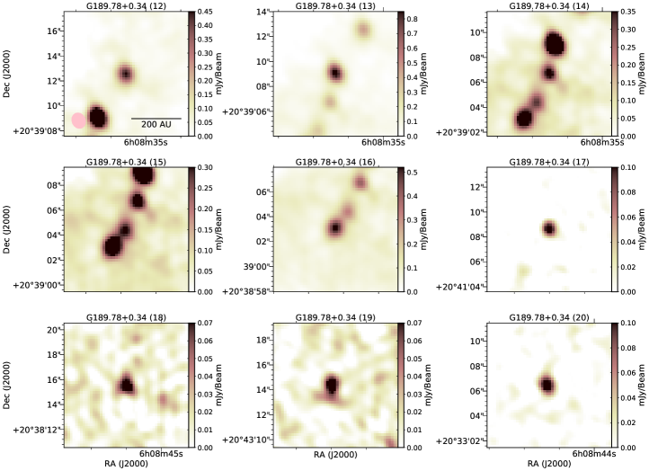
Figure 21: Close-up views of the C band (color scale image) and K band (contours) continuum images for the sources listed in Table LABEL:t:catalogue. Maps for the sources detected in region G189.78$+$0.34.

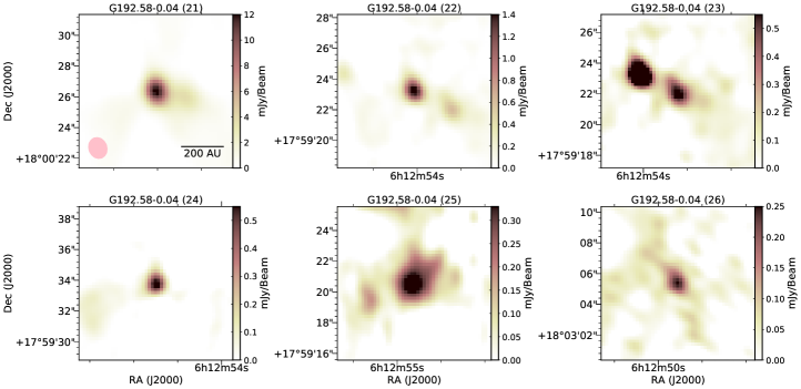
Figure 22: Close-up views of the C band (color scale image) and K band (contours) continuum images for the sources listed in Table LABEL:t:catalogue. Maps for the sources detected in region G192.58$-$0.04.

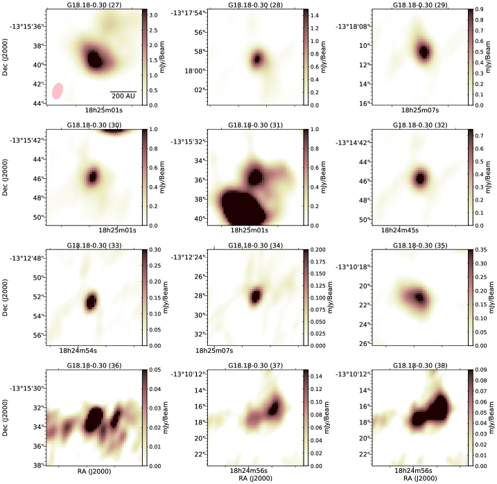
Figure 23: Close-up views of the C band (color scale image) and K band (contours) continuum images for the sources listed in Table LABEL:t:catalogue. Maps for the sources detected in region G18.18$-$0.30.

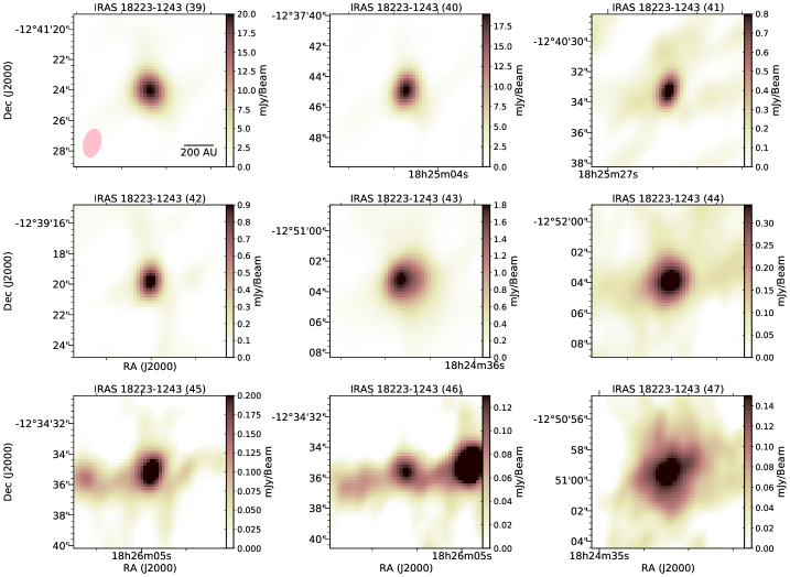
Figure 24: Close-up views of the C band (color scale image) and K band (contours) continuum images for the sources listed in Table LABEL:t:catalogue. Maps for the sources detected in region IRAS 18223$-$1243.

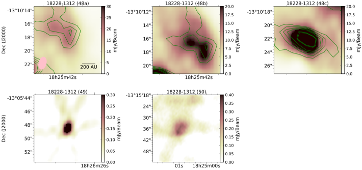
Figure 25: Close-up views of the C band (color scale image) and K band (contours) continuum images for the sources listed in Table LABEL:t:catalogue. Maps for the sources detected in region IRAS 18228$-$1312.

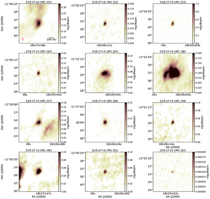
Figure 26: Close-up views of the C band (color scale image) and K band (contours) continuum images for the sources listed in Table LABEL:t:catalogue. Maps for the sources detected in region G19.27$+$0.1 M1.

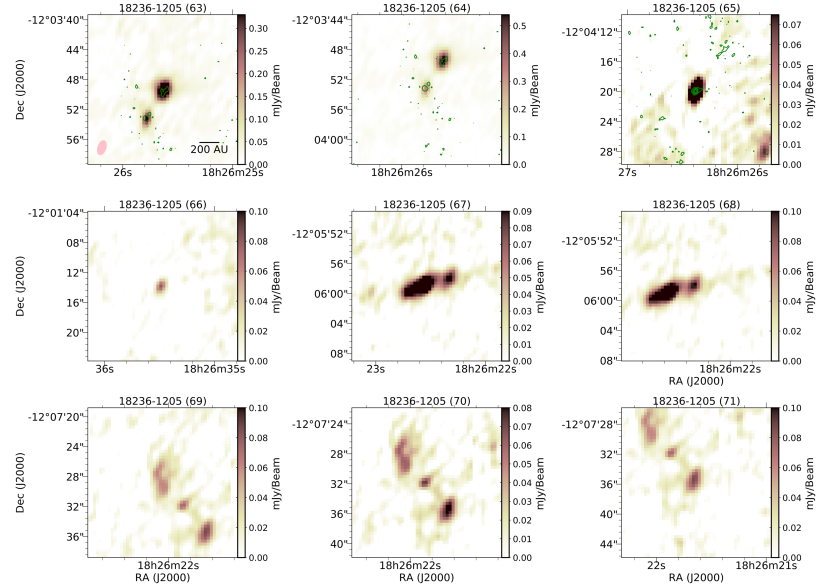
Figure 27: Close-up views of the C band (color scale image) and K band (contours) continuum images for the sources listed in Table LABEL:t:catalogue. Maps for the sources detected in region IRAS 18236$-$1205.

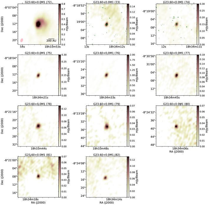
Figure 28: Close-up views of the C band (color scale image) and K band (contours) continuum images for the sources listed in Table LABEL:t:catalogue. Maps for the sources detected in region G23.60$+$0.0 M1.

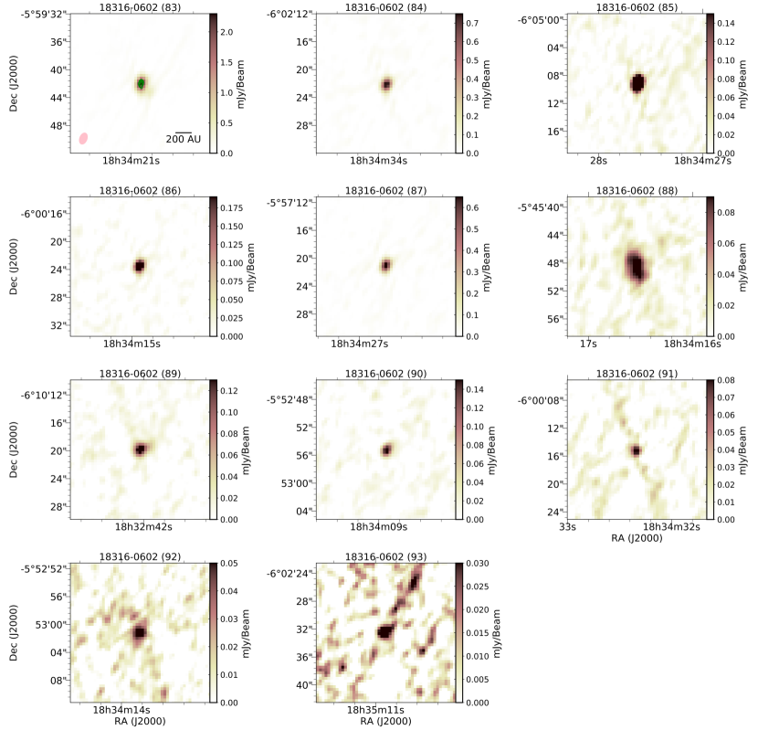
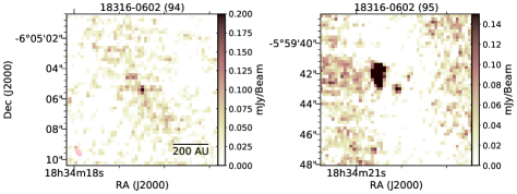
Figure 29: Close-up views of the C band (color scale image) and K band (contours) continuum images for the sources listed in Table LABEL:t:catalogue. The image of sources #94 and #95 correspond to the K band maps. Maps for the sources detected in region IRAS 18316$-$0602.

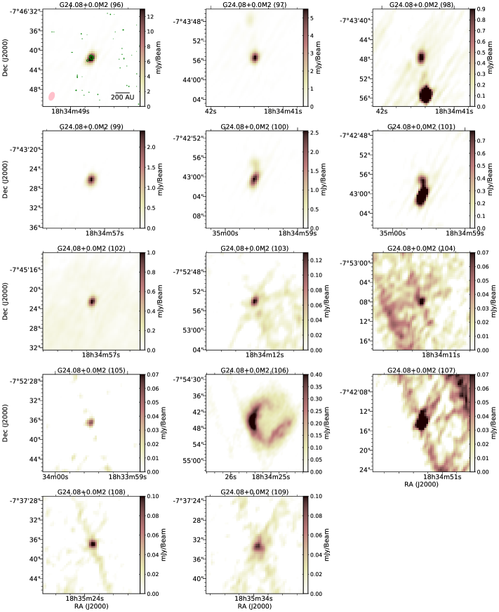
Figure 30: Close-up views of the C band (color scale image) and K band (contours) continuum images for the sources listed in Table LABEL:t:catalogue. Maps for the sources detected in region G24.08$+$0.0 M2.

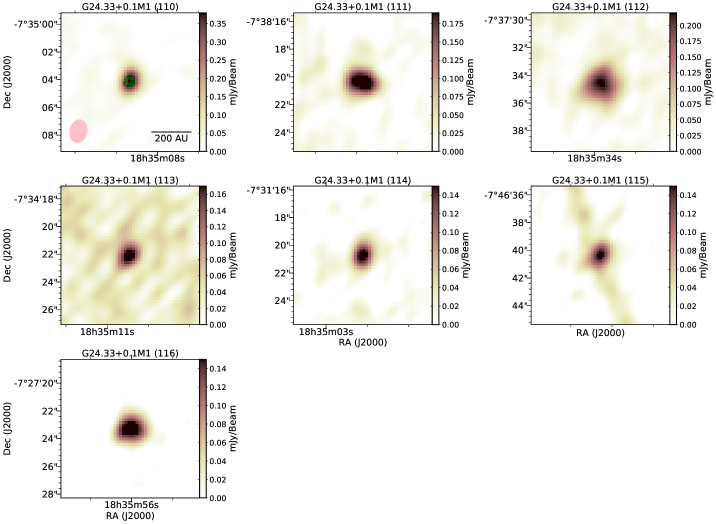
Figure 31: Close-up views of the C band (color scale image) and K band (contours) continuum images for the sources listed in Table LABEL:t:catalogue. Maps for the sources detected in region G24.33$+$0.1 M1.

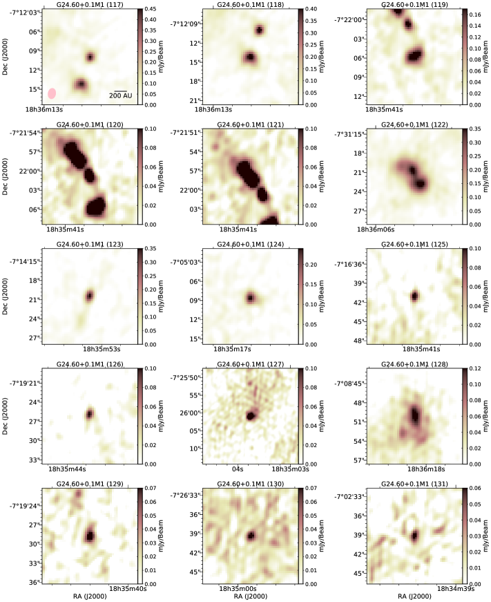
Figure 32: Close-up views of the C band (color scale image) and K band (contours) continuum images for the sources listed in Table LABEL:t:catalogue. Maps for the sources detected in region G24.60$+$0.1 M1.

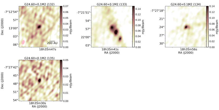
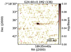
Figure 33: Close-up views of the C band (color scale image) and K band (contours) continuum images for the sources listed in Table LABEL:t:catalogue. The image of source #136 corresponds to the K band map. Maps for the sources detected in region G24.60$+$0.1 M2.

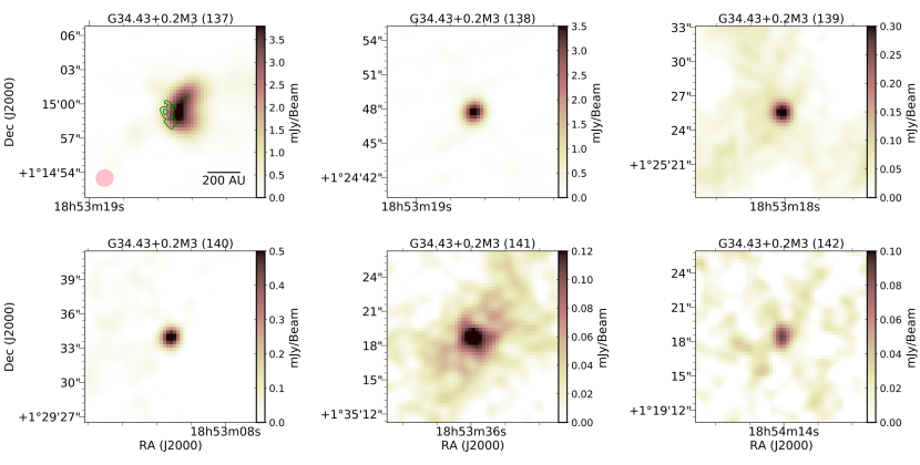
Figure 34: Close-up views of the C band (color scale image) and K band (contours) continuum images for the sources listed in Table LABEL:t:catalogue. Maps for the sources detected in region G34.43$+$0.2 M3.

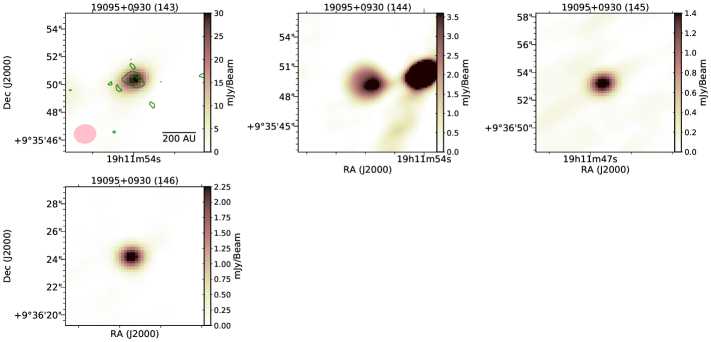
Figure 35: Close-up views of the C band (color scale image) and K band (contours) continuum images for the sources listed in Table LABEL:t:catalogue. Maps for the sources detected in region IRAS 19095$+$0930.