New physics in $b\rightarrow se^{+}e^{-}$: A model independent analysis

Abstract

The lepton universality violating flavor ratios $R_{K}/R_{K^{*}}$ indicate new physics either in $b\to s\mu^{+}\mu^{-}$ or in $b\to se^{+}e^{-}$ or in both. If the new physics is only $b\to se^{+}e^{-}$ transition, the corresponding new physics operators, in principle, can have any Lorentz structure. In this work, we perform a model independent analysis of new physics only in $b\to se^{+}e^{-}$ decay by considering effective operators either one at a time or two similar operators at a time. We include all the measurements in $b\rightarrow se^{+}e^{-}$ sector along with $R_{K}/R_{K^{*}}$ in our analysis. We show that various new physics scenarios with vector/axial-vector operators can account for $R_{K}/R_{K^{*}}$ data but those with scalar/pseudoscalar operators and with tensor operators can not. We also show that the azimuthal angular observable $P_{1}$ in $B\to K^{*}e^{+}e^{-}$ decay is most suited to discriminate between the different allowed solutions.

I Introduction

The current measurements in $b\to s\ell^{+}\ell^{-}$ ($\ell=e,\,\mu$) sector show some significant tensions with the predictions of the Standard Model (SM). These include measurements of the lepton flavor universality (LFU) violating ratios $R_{K}$ and $R_{K^{*}}$ by the LHCb collaboration. In 2014, the LHCb collaboration reported the first measurement of the ratio $R_{K}\equiv\Gamma(B^{+}\to K^{+}\mu^{+}\mu^{-})/\Gamma(B^{+}\to K^{+}e^{+}e^{-})$ in the di-lepton invariant mass-squared, $q^{2}$, range $1.1\leq q^{2}\leq 6.0$ GeV² rk . The measured value $0.745^{+0.090}_{-0.074}(\rm stat.)\pm 0.036(\rm syst.)$ deviates from the SM prediction of $\approx 1$ Hiller:2003js ; Bordone:2016gaq ; Bouchard:2013mia by 2.6$\sigma$ . Including the Run-II data and an update of the Run-I analysis, the value of $R_{K}$ was updated in Moriond-2019. The updated value $0.846^{+0.060}_{-0.054}\,(\rm stat.)^{+0.016}_{-0.014}({\rm syst.})$ Aaij:2019wad is still $\simeq 2.5\sigma$ away from the SM.

The hint of LFU violation is further observed in another flavor ratio $R_{K^{*}}$. This ratio $R_{K^{*}}\equiv\Gamma(B^{0}\to K^{*0}\mu^{+}\mu^{-})/\Gamma(B^{0}\to K^{*0}e^{+}e^{-})$ was measured in the low ($0.045\leq q^{2}\leq 1.1$ GeV²) as well as in the central ($1.1\leq q^{2}\leq 6.0$ GeV²) $q^{2}$ bins by the LHCb collaboration Aaij:2017vbb . The measured values are $0.660^{+0.110}_{-0.070}(\rm stat.)\pm 0.024(\rm syst.)$ for the low $q^{2}$ bin and $0.685^{+0.113}_{-0.069}(\rm stat.)\pm 0.047(\rm syst.)$ for the central $q^{2}$ bin. These measurements differ from the SM predictions of $R_{K^{*}}^{\rm low}=0.906\pm 0.028$ and $R_{K^{*}}^{\rm central}=1.00\pm 0.01$ Bordone:2016gaq by $\sim 2.5\sigma$ and $\sim 3\sigma$, respectively. Later Belle collaboration announced their first results on the measurements of $R_{K^{*}}$ in different $q^{2}$ bins for both $B^{0}$ and $B^{+}$ decay modes Abdesselam:2019wac . The measured values suffer from large statistical uncertainties and hence consistent with the SM predictions. The ratios $R_{K}$ and $R_{K^{*}}$ are essentially free from the hadronic uncertainties, making them extremely sensitive to new physics (NP) in $b\rightarrow se^{+}e^{-}$ or/and $b\rightarrow s\mu^{+}\mu^{-}$ transition(s).

Further, there are a few anomalous measurements which are related to possible NP in $b\to s\mu^{+}\mu^{-}$ transition only. These include measurements of angular observables, in particular $P^{\prime}_{5}$, in $B\to K^{*}\,\mu^{+}\,\mu^{-}$ decay Kstarlhcb1 ; Kstarlhcb2 ; Aaij:2020nrf and the branching ratio of $B_{s}\to\phi\,\mu^{+}\,\mu^{-}$ bsphilhc2 . By virtue of these measurements, it is natural to assume NP only in the muon sector to accommodate all $b\to s\ell^{+}\ell^{-}$ data. A large number of global analyses of $b\to s\ell^{+}\ell^{-}$ data have been performed under this assumption Alguero:2019ptt ; Alok:2019ufo ; Ciuchini:2019usw ; DAmico:2017mtc ; Aebischer:2019mlg ; Kowalska:2019ley ; Arbey:2019duh . NP amplitude in $b\to s\mu^{+}\mu^{-}$ must have destructive interference with the SM amplitude to account for $R_{K},R_{K^{*}}<1$. Hence the NP operators in this sector are constrained to be in vector/axial-vector form. The global analyses found three different combinations of such operators which can account for all the data. Possible methods to distinguish between these allowed NP solutions are investigated in refs. Kumar:2017xgl ; Kumbhakar:2018uty ; Alok:2020bia ; Bhutta:2020qve . However, the predicted value of $R_{K^{*}}^{\rm low}$ for the solutions with NP only in $b\to s\mu^{+}\mu^{-}$ still differs significantly from the measured value. This requires presence of NP in $b\rightarrow se^{+}e^{-}$ along with $b\rightarrow s\mu^{+}\mu^{-}$, see for e.g, Kumar:2019qbv ; Datta:2019zca .

While the LFU ratios $R_{K}$ and $R_{K^{*}}$ are theoretically clean, other observables in $b\to s\mu^{+}\mu^{-}$ sector which show discrepancy with SM, in particular the angular observables $B\to K^{*}\mu^{+}\mu^{-}$ and $B_{s}\to\phi\mu^{+}\mu^{-}$, are subject to significant hadronic uncertainties dominated by undermined power corrections. So far, the power corrections can be estimated only in the inclusive decays. For exclusive decays, there are no theoretical description of power corrections within QCD factorization and SCET framework. The possible NP effects in these observables can be masked by such corrections. The disagreement with the SM depends upon the guess value of power corrections. Under the assumption of $\rm\sim 10\%$ non-factorisable power corrections in the SM predictions, the measurements of these observables show deviations from the SM at the level of 3-4$\sigma$. However, if one assumes a sizable non-factorisable power corrections, the experimental data can be accommodated within the SM itself Ciuchini:2015qxb ; Hurth:2016fbr ; Chobanova:2017ghn ; Hurth:2020rzx . It is therefore expected that these tensions might stay unexplained until Belle-II can measure the corresponding observables in the inclusive $b\to s\mu^{+}\mu^{-}$ modes Hurth:2016fbr .

Therefore, if one considers the discrepancies in clean observables in $b\to s\ell^{+}\ell^{-}$ sector, which are $R_{K}$ and $R_{K^{*}}$, then NP only in $b\rightarrow se^{+}e^{-}$ is as natural solution as NP in $b\rightarrow s\mu^{+}\mu^{-}$ sector. In this work, we consider this possibility and perform a model independent analysis with NP restricted to $b\rightarrow se^{+}e^{-}$ sector . In this scenario, we need the NP operators to increase the denominators of $R_{K}$ and $R_{K^{*}}$. Hence, the need for interference with SM amplitude is no longer operative. We consider NP in the form of vector/axial-vector (V/A), scalar/pseudoscalar (S/P) and tensor (T) operators. We show that solutions based on V/A operators predict values of $R_{K}/R_{K^{*}}$, including $R_{K^{*}}^{\rm low}$, which are in good agreement with the measured values. The scalar NP operators can account for the reduction in $R_{K}$ but not in $R_{K^{*}}$ and hence are ruled out. The coefficients of pseudoscalar operators are very severely constrained by the current bound on the branching ratio of $B_{s}\to e^{+}e^{-}$ and these operators do not lead to a reduction of $R_{K}/R_{K^{*}}$. It is not possible to get a solution to the $R_{K}/R_{K^{*}}$ problem using only tensor operators Hiller:2014yaa but a solution is possible in the form of a combination of V/A and T operators, as shown in ref. Bardhan:2017xcc . In this work, we will limit ourselves to solutions involving either one NP operator or two similar NP operators at a time. We will not consider solutions with two or more dissimilar operators.

The paper is organized as follows. In Sec. II, we discuss the methodology adopted in this work. The fit results for NP in the form of V/A operators are shown in Sec. III. In Sec. III.1, we discuss methods to discriminate between different V/A solutions and comment on the most effective angular observables which can achieve this discrimination. Finally, we present our conclusions in Sec.  IV.

II Methodology

We analyze the $R_{K}/R_{K^{*}}$ anomalies within the framework of effective field theory (EFT) by assuming NP only in $b\to se^{+}e^{-}$ transition. We intend to identify the set of operators which can account for the measurements of $R_{K}/R_{K^{*}}$. We consider NP in the form of V/A, S/P and T operators and analyze scenarios with either one NP operator (1D) at a time or two similar NP operators (2D) at a time.

In the SM, the effective Hamiltonian for $b\to s\ell^{+}\ell^{-}$ transition is

$$\mathcal{H}^{\rm SM} = -\frac{4G_{F}}{\sqrt{2}\pi}V_{ts}^{*}V_{tb}\left[\sum_{i=1}^{6}C_{i}(\mu)\mathcal{O}_{i}(\mu)+C_{7}\frac{e}{16\pi^{2}}[\overline{s}\sigma_{\mu\nu}(m_{s}P_{L}+m_{b}P_{R})b]F^{\mu\nu}\right.$$ (1)

$$\left.+C_{9}\frac{\alpha_{em}}{4\pi}(\overline{s}\gamma^{\mu}P_{L}b)(\overline{\ell}\gamma_{\mu}\ell)+C_{10}\frac{\alpha_{em}}{4\pi}(\overline{s}\gamma^{\mu}P_{L}b)(\overline{\ell}\gamma_{\mu}\gamma_{5}\ell)\right],$$

where $G_{F}$ is the Fermi constant, $V_{ts}$ and $V_{tb}$ are the Cabibbo-Kobayashi-Maskawa (CKM) matrix elements and $P_{L,R}=(1\mp\gamma^{5})/2$ are the projection operators. The effect of the operators $\mathcal{O}_{i},\,i=1-6,8$ can be embedded in the redefined effective Wilson coefficients (WCs) as $C_{7}(\mu)\rightarrow C^{\rm eff}_{7}(\mu,q^{2})$ and $C_{9}(\mu)\rightarrow C^{\rm eff}_{9}(\mu,q^{2})$.

We now add following NP contributions to the SM effective Hamiltonian,

$$\mathcal{H}^{\rm NP}_{\rm VA} = -\frac{\alpha_{\rm em}G_{F}}{\sqrt{2}\pi}V_{ts}^{*}V_{tb}\left[C^{\rm NP,\,e}_{9}\,(\overline{s}\gamma^{\mu}P_{L}b)\,(\overline{e}\gamma_{\mu}e)+C^{\rm NP,\,e}_{10}\,(\overline{s}\gamma^{\mu}P_{L}b)\,(\overline{e}\gamma_{\mu}\gamma_{5}e)\right.$$ (2)

$$+\left.C^{\prime,\,\rm e}_{9}\,(\overline{s}\gamma^{\mu}P_{R}b)\,(\overline{e}\gamma_{\mu}e)+C^{\prime,\,\rm e}_{10}\,(\overline{s}\gamma^{\mu}P_{R}b)\,(\overline{e}\gamma_{\mu}\gamma_{5}e)\right],$$

$$\mathcal{H}^{\rm NP}_{\rm SP} = -\frac{\alpha_{\rm em}G_{F}}{\sqrt{2}\pi}V^{*}_{ts}V_{tb}\left[C^{\rm e}_{SS}\,(\overline{s}b)(\overline{e}e)+C^{\rm e}_{SP}\,(\overline{s}b)(\overline{e}\gamma_{5}e)\right.$$ (3)

$$+\left.C^{\rm e}_{PS}\,(\overline{s}\gamma_{5}b)\,(\overline{e}e)+C^{\rm e}_{PP}\,(\overline{s}\gamma_{5}b)\,(\overline{e}\gamma_{5}e)\right],$$

$$\mathcal{H}^{\rm NP}_{\rm T} = -\frac{\alpha_{\rm em}G_{F}}{\sqrt{2}\pi}V^{*}_{ts}V_{tb}\left[C^{\rm e}_{T}\,(\overline{s}\sigma^{\mu\nu}b)\,(\overline{e}\sigma_{\mu\nu}e)+C^{\rm e}_{T5}\,(\overline{s}\sigma^{\mu\nu}b)\,(\overline{e}\sigma_{\mu\nu}\gamma_{5}e)\right],$$ (4)

where $C^{\rm NP,\,e}_{9,10}$, $C^{\prime,\,\rm e}_{9,10}$, and $C^{\rm e}_{SS,SP,PS,PP,T,T5}$ are the NP WCs.

Using simple symmetry arguments, we can argue that S/P operators can not provide a solution to $R_{K}/R_{K^{*}}$ discrepancy. The operators containing the quark bilinear $\bar{s}b$ can lead to $B\to Ke^{+}e^{-}$ transition but not $B\to K^{*}e^{+}e^{-}$ transition. Such operators can account for $R_{K}$ but not $R_{K^{*}}$. On the other hand, the operators containing the quark pseudoscalar bilinear $\overline{s}\gamma_{5}b$ can not lead to $B\to Ke^{+}e^{-}$. These operators can not account for $R_{K}$. In addition, the contribution of these operators to $B_{s}\to e^{+}e^{-}$ is not subject to helicity suppression. Hence, the coefficients $C^{\rm e}_{PS}$ and $C^{\rm e}_{PP}$ are constrained to be very small. The current upper limit on $\mathcal{B}(B_{s}\to e^{+}e^{-})<9.4\times 10^{-9}$ at $90\%$ C.L., leads to the condition

$$|C^{\rm e}_{PS}|^{2}+|C^{\rm e}_{PP}|^{2}\lesssim 0.01,$$ (5)

whereas one needs

$$120\lesssim|C^{\rm e}_{PS}|^{2}+|C^{\rm e}_{PP}|^{2}\lesssim 345,\quad\,9\lesssim|C^{\rm e}_{PS}|^{2}+|C^{\rm e}_{PP}|^{2}\lesssim 29,$$ (6)

to satisfy the experimental constraint on $R^{\rm low}_{K^{*}}$ and $R^{\rm central}_{K^{*}}$ respectively. Therefore, we will not consider S/P operators in our fit procedure.

The NP Hamiltonian can potentially impact observables in the decays induced by the quark level transition $b\to se^{+}e^{-}$. To obtain the values of NP WCs, we perform a fit to the current data in $b\to se^{+}e^{-}$ sector. We consider following fifteen observables in our fit:

• Measured values of $R_{K}$ in $1.1\leq q^{2}\leq 6.0$ GeV² bin  Aaij:2019wad and $R_{K^{*}}$ in both $0.045<q^{2}<1.1$ GeV² and $1.1<q^{2}<6.0$ GeV² bins by the LHCb collaboration Aaij:2017vbb ,

• Measured values of $R_{K^{*}}$ by the Belle collaboration in $0.045<q^{2}<1.1$ GeV², $1.1<q^{2}<6.0$ GeV² and $15.0<q^{2}<19.0$ GeV² bins for both $B^{0}$ and $B^{+}$ decay modes Abdesselam:2019wac ,

• The upper limit of $\mathcal{B}(B_{s}\to e^{+}e^{-})<9.4\times 10^{-9}$ at $90\%$ C.L. by the LHCb collaboration (Aaij:2020nol, ),

• The differential branching fraction of $B\to K^{*}e^{+}e^{-}$, $(3.1^{+0.9}_{-0.8}\pm 0.2)\times 10^{-7}$, in $0.001<q^{2}<1.0$ GeV² bin by the LHCb collaboration Aaij:2013hha ,

• The measured value of $K^{*}$ longitudinal polarization fraction $F_{L}$, $0.16\pm 0.06\pm 0.03$, in $0.002<q^{2}<1.12$ GeV² bin by the LHCb collaboration Aaij:2015dea ,

• Measured values of the branching ratios of $B\to X_{s}e^{+}e^{-}$ by the BaBar collaboration in both $1.0<q^{2}<6.0$ GeV² and $14.2<q^{2}<25.0$ GeV² bins which are $\left(1.93^{+0.47+0.21}_{-0.45-0.16}\pm 0.18\right)\times 10^{-6}$ and $\left(0.56^{+0.19+0.03}_{-0.18-0.03}\right)\times 10^{-6}$, respectively Lees:2013nxa ,

• Measured values of $P^{\prime}_{4}$ in $B\to K^{*}e^{+}e^{-}$ decay by the Belle collaboration in $1.0<q^{2}<6.0$ GeV² and $14.18<q^{2}<19.0$ GeV² bins which are $-0.72^{+0.40}_{-0.39}\pm 0.06$ and $-0.15^{+0.41}_{-0.40}\pm 0.04$, respectively Wehle:2016yoi ,

• Measured values of $P^{\prime}_{5}$ in $B\to K^{*}e^{+}e^{-}$ decay by the Belle collaboration in $1.0<q^{2}<6.0$ GeV² and $14.18<q^{2}<19.0$ GeV² bins which are $-0.22^{+0.39}_{-0.41}\pm 0.03$ and $-0.91^{+0.36}_{-0.30}\pm 0.03$, respectively  Wehle:2016yoi .

We define the $\chi^{2}$ function as

$$\chi^{2}(C_{i})=\sum_{\rm all\,obs.}\frac{\left(O^{\rm th}(C_{i})-O^{\rm exp}\right)^{2}}{\sigma^{2}_{\rm exp}+\sigma^{2}_{\rm th}}.$$ (7)

Here $O^{\rm th}(C_{i})$ are the theoretical predictions of the observables taken into fit which depend on the NP WCs and $O^{\rm exp}$ are the measured central values of the corresponding observables. The $\sigma_{\rm exp}$ and $\sigma_{\rm th}$ are the experimental and theoretical uncertainties, respectively. The experimental errors in all observables dominate over the theoretical errors. In case of the asymmetric errors, we use the larger error in our analysis. The prediction of $O^{\rm th}(C_{i})$ is obtained using Flavio package Straub:2018kue which uses the most precise form factor predictions obtained in the light cone sum rule (LCSR) Straub:2015ica ; Gubernari:2018wyi approach. The non-factorisable corrections are incorporated following the parameterization used in Ref. Straub:2015ica ; Straub:2018kue . These are also compatible with the calculations in Ref. Khodjamirian:2010vf ; Gubernari:2020eft .

We obtain the values of NP WCs by minimizing the $\chi^{2}$ using CERN minimization code Minuit James:1975dr ; James:1994vla . We perform the minimization in two ways: (a) one NP operator at a time and (b) two NP operators at a time. Since we do the fit with fifteen data points, it is expected that an NP scenario with a value of $\chi^{2}_{\rm min}\approx 15$ provides a good fit to the data. We also define pull $=\sqrt{\Delta\chi^{2}}$ where $\Delta\chi^{2}=(\chi^{2}_{\rm SM}-\chi^{2}_{\rm min})$. Since $\chi^{2}_{\rm SM}\approx 27$, any scenario with pull $\gtrsim 3.0$ can be considered to be a viable solution. In the next section, we present our fit results and discuss them in details.

III Vector/axial-vector new physics

There are four cases for one operator fit and six cases for two operators fit. For all of these cases, we list the best fit values of WCs in Table 1 along with their $\chi^{2}_{\rm min}$ values. We also calculate the corresponding values of pull which determine the degree of improvement over the SM.

Wilson Coefficient(s)	Best fit value(s)	$\chi^{2}_{\rm min}$	pull
$C_{i}=0$ (SM)	$-$	27.42
1D Scenarios
$C^{\rm NP,e}_{9}$	$0.91\pm 0.28$	15.21	3.5
$C^{\rm NP,e}_{10}$	$-0.86\pm 0.25$	12.60	3.8
$C^{\prime,e}_{9}$	$0.24\pm 0.24$	26.40	1.0
$C^{\prime,e}_{10}$	$-0.17\pm 0.21$	26.70	0.8
2D Scenarios
$(C^{\rm NP,e}_{9},C^{\rm NP,e}_{10})$	$(-1.03,-1.42)$	11.57	3.9
$(C^{\rm NP,e}_{9},C^{\prime,e}_{9})$	$(-3.61,-4.76)$	17.65	3.1
	$(-3.52,4.29)$	15.71	3.4
	$(1.21,-0.54)$	12.83	3.8
$(C^{\rm NP,e}_{9},C^{\prime,e}_{10})$	$(1.21,0.69)$	12.39	3.9
$(C^{\prime,e}_{9},C^{\rm NP,e}_{10})$	$(-0.50,-1.03)$	11.30	4.0
$(C^{\prime,e}_{9},C^{\prime,e}_{10})$	$(2.05,2.33)$	10.41	4.1
	$(-2.63,-1.86)$	12.71	3.8
$(C^{\rm NP,e}_{10},C^{\prime,e}_{10})$	$(3.64,5.33)$	18.50	3.0
	$(-1.04,0.38)$	11.14	4.0
	$(4.56,-5.24)$	16.58	3.3

Table 1: The best fit values of NP WCs in $b\rightarrow se^{+}e^{-}$ transition for 1D and 2D scenarios. The value of $\chi^{2}_{\rm SM}$ is 27.42.

From Table 1, we find that the $C_{9}^{\rm NP,e}$ and $C_{10}^{\rm NP,e}$ scenarios provide a good fit to the $b\to se^{+}e^{-}$ data. However, the other two 1D scenarios, $C_{9}^{\prime,e}$ and $C_{10}^{\prime,e}$, fail to provide any improvement over the SM. Therefore, we reject them on the basis of $\Delta\chi^{2}$ or pull. In the case of 2D framework, all six combinations improve the global fit as compared to the SM.

We now impose the stringent condition that a NP solution must predict the values of $R_{K}$, $R^{\rm low}_{K^{*}}$ and $R^{\rm central}_{K^{*}}$ to be within 1$\sigma$ of their measured values. In order to identify solutions satisfying this condition, we calculate the predictions of $R_{K}/R_{K^{*}}$ for all good fit scenarios. The predicted values of these quantities are listed in Table 2 from which we observe that the 1D scenario $C_{9}^{\rm NP}$ could not accommodate both the $R^{\rm low}_{K^{*}}$ and $R^{\rm central}_{K^{*}}$ within $1\sigma$ whereas most of the other solutions fail to explain the $1\sigma$ range of $R^{\rm low}_{K^{*}}$ only. There are only three 2D solutions whose predictions for $R_{K}$, $R^{\rm low}_{K^{*}}$ and $R^{\rm central}_{K^{*}}$ are within $1\sigma$ of their measurements. We call these scenarios as allowed NP solutions and list them in Table 3. The $1\sigma$ and $2\sigma$ allowed regions for these three allowed solutions are shown in Fig 1.

Wilson Coefficient(s)	Best fit value(s)	pull	$R_{K}$	$R^{\rm low}_{K^{*}}$	$R^{\rm central}_{K^{*}}$
Expt. $1\sigma$ range			$[0.784,0.908]$	$[0.547,0.773]$	$[0.563,0.807]$
1D Scenarios
$C^{\rm NP,e}_{9}$	$0.91\pm 0.28$	3.5	$0.806\pm 0.001$	$0.883\pm 0.008$	$0.832\pm 0.009$
$C^{\rm NP,e}_{10}$	$-0.86\pm 0.25$	3.8	$0.805\pm 0.005$	$0.855\pm 0.007$	$0.778\pm 0.012$
2D Scenarios
$(C^{\rm NP,e}_{9},C^{\rm NP,e}_{10})$	$(-1.03,-1.42)$	3.9	$0.825\pm 0.011$	$0.832\pm 0.007$	$0.745\pm 0.026$
$(C^{\rm NP,e}_{9},C^{\prime,e}_{9})$	$(-3.61,-4.76)$	3.1	$0.867\pm 0.050$	$0.757\pm 0.007$	$0.625\pm 0.024$
	$(-3.52,4.29)$	3.4	$0.832\pm 0.001$	$0.798\pm 0.028$	$0.707\pm 0.090$
	$(1.21,-0.54)$	3.8	$0.853\pm 0.001$	$0.825\pm 0.018$	$0.701\pm 0.012$
$(C^{\rm NP,e}_{9},C^{\prime,e}_{10})$	$(1.21,0.69)$	3.9	$0.855\pm 0.004$	$0.819\pm 0.016$	$0.691\pm 0.011$
$(C^{\prime,e}_{9},C^{\rm NP,e}_{10})$	$(-0.50,-1.03)$	4.0	$0.844\pm 0.007$	$0.812\pm 0.012$	$0.690\pm 0.009$
$(C^{\prime,e}_{9},C^{\prime,e}_{10})$	$(2.05,2.33)$	4.1	$0.845\pm 0.010$	$0.808\pm 0.014$	$0.683\pm 0.029$
	$(-2.63,-1.86)$	3.8	$0.856\pm 0.020$	$0.808\pm 0.015$	$0.684\pm 0.010$
$(C^{\rm NP,e}_{10},C^{\prime,e}_{10})$	$(3.64,5.33)$	3.0	$0.860\pm 0.015$	$0.788\pm 0.014$	$0.645\pm 0.015$
	$(-1.04,0.38)$	4.0	$0.846\pm 0.004$	$0.809\pm 0.013$	$0.686\pm 0.014$
	$(4.56,-5.24)$	3.3	$0.842\pm 0.004$	$0.809\pm 0.015$	$0.685\pm 0.019$

Table 2: The predictions of $R_{K}$, $R^{\rm low}_{K^{*}}$ and $R^{\rm central}_{K^{*}}$ for the good fit scenarios obtained in Table. 1.

Solution	Wilson Coefficient(s)	Best fit value(s)	pull	$R_{K}$	$R^{\rm low}_{K^{*}}$	$R^{\rm central}_{K^{*}}$
Expt. $1\sigma$ range				$[0.784,0.908]$	$[0.547,0.773]$	$[0.563,0.807]$
2D Scenarios
I	$(C^{\rm NP,e}_{9},C^{\prime,e}_{9})$	$(-3.61,-4.76)$	3.1	$0.867\pm 0.050$	$0.757\pm 0.007$	$0.625\pm 0.024$
II		$(-3.52,4.29)$	3.4	$0.832\pm 0.001$	$0.798\pm 0.028$	$0.707\pm 0.090$
III	$(C^{\rm NP,e}_{10},C^{\prime,e}_{10})$	$(3.64,5.33)$	3.0	$0.860\pm 0.015$	$0.788\pm 0.014$	$0.645\pm 0.015$

Table 3: Here we list only those NP WCs which generate $R_{K}$ and $R_{K^{*}}$ within $1\sigma$ range of their experimental values.

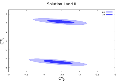
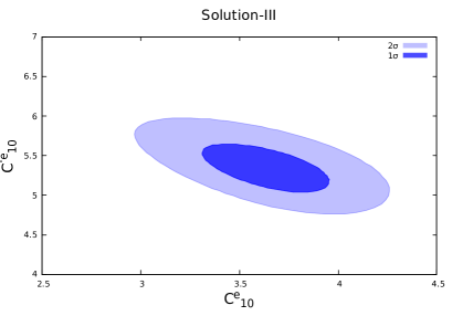
Figure 1: The allowed $1\sigma$ and $2\sigma$ ellipses for the three 2D solutions listed in Table 3.

The EFT analysis can serve as a guideline for constructing NP models. A detailed analysis of possible models which can generate the favoured Lorentz structure obtained above is beyond the scope of this work. Here we briefly discuss some of the simple models which can generate these scenarios at the tree level. The pattern of NP obtained through the above model independent analysis can be realised in those NP models where $b\to s\mu^{+}\mu^{-}$ transition remains SM like. Hence models based on $L_{\mu}-L_{\tau}$ gauge symmetry Heeck:2011wj ; Altmannshofer:2014cfa ; Crivellin:2015mga ; Altmannshofer:2015mqa ; Crivellin:2016ejn as well as partial compositeness Niehoff:2015bfa would not generate the allowed Lorentz structures as these models naturally generate NP effects in the muon sector, while keeping $b\to se^{+}e^{-}$ SM like. The allowed EFT scenarios can be generated in a $Z^{\prime}$ model with coupling only to electrons and avoiding LEP constraints. For e.g., a light $Z^{\prime}$ ($M_{Z^{\prime}}\sim$ 25 MeV) with a $q^{2}$ dependent $b-s$ coupling that couples to the electron but not to the muons can induce the favored operators Datta:2017ezo . Another alternative would be a class of scalar or vector leptoquark models with coupling only to electrons along with flavor-changing quark couplings, see for e.g., Hiller:2014yaa ; DAmico:2017mtc ; Dorsner:2016wpm .

After identifying the allowed solutions, we find out the set of observables which can discriminate between them. In the next subsection, we investigate discriminating capabilities of the standard angular observables in $B\to K^{*}e^{+}e^{-}$ decay.

III.1 Discriminating V/A solutions

The differential distribution of the four-body decay $B\to K^{*}(\to K\pi)e^{+}e^{-}$ can be parametrized as the function of one kinematic ($q^{2}$) and three angular variables $\overrightarrow{\Omega}=(\cos\theta_{K},\cos\theta_{e},\phi)$. The kinematic variable is $q^{2}=(p_{B}-p_{K^{*}})^{2}$, where $p_{B}$ and $p_{K^{*}}$ are respective four-momenta of $B$ and $K^{*}$ mesons. The angular variables are defined in the $K^{*}$ rest frame. They are (a) $\theta_{K}$ the angle between $B$ and $K$ mesons where $K$ meson comes from $K^{*}$ decay, (b) $\theta_{e}$ the angle between momenta of $e^{-}$ and $B$ meson and (c) $\phi$ the angle between $K^{*}$ decay plane and the plane defined by the $e^{+}-e^{-}$ momenta. The CP averaged angular distribution of the $B\to K^{*}(\to K\pi)e^{+}e^{-}$ decay can be written as Aaij:2015oid

$$\frac{1}{d(\Gamma+\bar{\Gamma})/dq^{2}}\frac{d^{4}(\Gamma+\bar{\Gamma})}{dq^{2}d\overrightarrow{\Omega}} = \frac{9}{32\pi}\left[\frac{3}{4}\left(1-F_{L}\right)\sin^{2}\theta_{K}+F_{L}\cos^{2}\theta_{K}+\frac{1}{4}(1-F_{L})\sin^{2}\theta_{K}\cos 2\theta_{e}\right.$$ (8)

$$-F_{L}\cos^{2}\theta_{K}\cos 2\theta_{e}+S_{3}\sin^{2}\theta_{K}\sin^{2}\theta_{e}\cos 2\phi$$

$$+S_{4}\sin 2\theta_{K}\sin 2\theta_{e}\cos\phi+S_{5}\sin 2\theta_{K}\sin\theta_{e}\cos\phi$$

$$+\frac{4}{3}A_{FB}\sin^{2}\theta_{K}\cos\theta_{e}+S_{7}\sin 2\theta_{K}\sin\theta_{e}\sin\phi$$

$$+S_{8}\sin 2\theta_{K}\sin 2\theta_{e}\sin\phi+S_{9}\sin^{2}\theta_{K}\sin^{2}\theta_{e}\sin 2\phi\Big{]}.$$

Following the notations of ref. Altmannshofer:2008dz , the $q^{2}$ dependent $CP$ averaged angular observables $S_{i}$ can be defined as

$$S_{i}(q^{2})=\frac{I_{i}(q^{2})+\bar{I}_{i}(q^{2})}{d(\Gamma+\bar{\Gamma})/dq^{2}}.$$ (9)

The detailed expressions of angular coefficients $I_{i}$ can also be found in ref. Altmannshofer:2008dz .

The longitudinal polarization fraction of $K^{*}$, $F_{L}$, depends on the distribution of the events in the angle $\theta_{K}$ (after integrating over $\theta_{e}$ and $\phi$) and the forward-backward asymmetry, $A_{FB}$, is defined in terms of $\theta_{e}$ (after integrating over $\theta_{K}$ and $\phi$). We can write these two quantities in terms of $S^{(a)}_{i}$ as follows Altmannshofer:2008dz

$$A_{FB}=\frac{3}{8}\left(2S^{s}_{6}+S^{c}_{6}\right),\quad F_{L}=-S^{c}_{2}.$$ (10)

In addition to the $S_{i}$ observables, one can also investigate the NP effects on a set of optimized observables $P_{i}$. In fact, the observables $P_{i}$ are theoretically cleaner in comparison to the form factors dependent observables $S_{i}$. These two sets of observables are related to each other DescotesGenon:2012zf . However, there are several notations used in the literature. The definition of the $P_{i}$ observables used in this work follows the LHCb convention Aaij:2015oid

$$P_{1}=\frac{2S_{3}}{1-F_{L}},\quad P_{2}=\frac{2}{3}\frac{A_{FB}}{(1-F_{L})},\quad P_{3}=\frac{-S_{9}}{1-F_{L}},$$

$$P^{\prime}_{4}=\frac{S_{4}}{\sqrt{F_{L}(1-F_{L})}},\quad P^{\prime}_{5}=\frac{S_{5}}{\sqrt{F_{L}(1-F_{L})}},\quad P^{\prime}_{6}=\frac{S_{7}}{\sqrt{F_{L}(1-F_{L})}},\quad P^{\prime}_{8}=\frac{S_{8}}{\sqrt{F_{L}(1-F_{L})}}.$$ (11)

The measurements of $P^{\prime}_{4}$ and $P^{\prime}_{5}$ observables by the Belle collaboration Wehle:2016yoi used in our fits also follow the LHCb notation. A complete relations between the LHCb definitions and the notations used in different papers can be found in ref. Gratrex:2015hna .

Observable	$q^{2}$ bin	SM	S-I	S-II	S-III
$A_{FB}$	$[1.1,6]$	$0.008\pm 0.031$	$-0.146\pm 0.026$	$-0.161\pm 0.027$	$-0.016\pm 0.011$
	$[15,19]$	$0.368\pm 0.018$	$-0.005\pm 0.003$	$0.002\pm 0.005$	$0.026\pm 0.004$
$F_{L}$	$[1.1,6]$	$0.764\pm 0.043$	$0.630\pm 0.056$	$0.599\pm 0.055$	$0.765\pm 0.042$
	$[15,19]$	$0.341\pm 0.020$	$0.338\pm 0.022$	$0.325\pm 0.020$	$0.349\pm 0.020$

Table 4: Average values of $B\to K^{*}e^{+}e^{-}$ angular observables $A_{FB}$ and $F_{L}$ in SM as well as for the allowed NP V/A solutions listed in Table. 3.

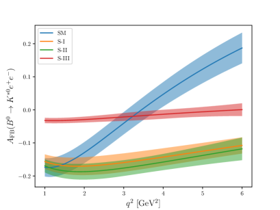
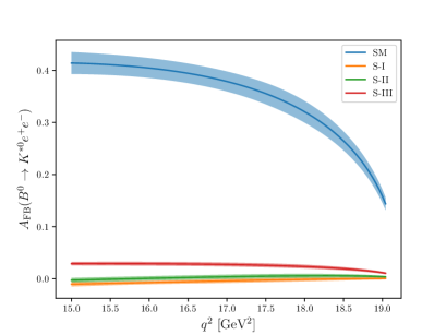
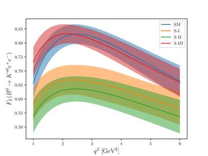
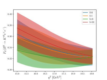
Figure 2: Plots of $A_{FB}$ and $F_{L}$ as a function of $q^{2}$ for the SM and the three NP V/A solutions. The left and right panels correspond to the low ($[1.1,6.0]$ GeV²) and high ($[15,19]$ GeV²) $q^{2}$ bins, respectively.

We calculate $A_{FB}$, $F_{L}$ along with optimized observables $P_{1,2,3}$ and $P^{\prime}_{4,5,6,8}$ for the SM and the three allowed NP solutions in $q^{2}\subset[1.1,6.0]$ and $[15,19]$ GeV² bins. The average values of $A_{FB}$ and $F_{L}$ are listed in Table 4 and the $q^{2}$ plots are shown in Fig. 2. From the predictions, we observe the following features:

• In low $q^{2}$ region, the SM prediction of $A_{FB}(q^{2})$ has a zero crossing at $\sim 3.5$ GeV². For the NP solutions, the predictions are negative throughout the low $q^{2}$ range. However, the $A_{FB}(q^{2})$ curve is almost the same for S-I and S-II whereas for S-III, it is markedly different. Therefore an accurate measurement of $q^{2}$ distribution of $A_{FB}$ can discriminate between S-III and the remaining two NP solutions.

• In high $q^{2}$ region, the SM prediction of $A_{FB}$ is $0.368\pm 0.018$ whereas the predictions for the three solutions are almost zero. If $A_{FB}$ in high $q^{2}$ region is measured to be small, it provides additional confirmation for the existence of NP, which is indicated by the reduced values of $R_{K}$ and $R_{K^{*}}$. All the three NP solutions induce a large deviation in $A_{FB}$, but the discriminating capability of $A_{FB}$ is extremely limited.

• The S-I and S-II scenarios can marginally suppress the value of $F_{L}$ in low $q^{2}$ region compared to the SM whereas for S-III, the predicted value is consistent with the SM. In high $q^{2}$ region, $F_{L}$ for all three scenarios are close to the SM value. Hence $F_{L}$ cannot discriminate between the allowed V/A solutions.

Hence we see that neither $A_{FB}$ nor $F_{L}$ have the power to discriminate between all the three allowed V/A NP solutions. Therefore, we now study optimized observables $P_{i}$ in $B\to K^{*}e^{+}e^{-}$ decay. In particular, we investigate the distinguishing ability of $P_{1,2,3}$ and $P^{\prime}_{4,5,6,8}$ . We compute the average values of these seven observables for the SM along with three NP scenarios in two different $q^{2}$ bins, $q^{2}\subset[1.1,6.0]$ and $[15,19]$ GeV². These are listed in Tab 5. We also plot these observables as a function of $q^{2}$ for the SM and the three solutions. The $q^{2}$ plots for $P_{1,2,3}$ and $P^{\prime}_{4,5,6,8}$ are illustrated in Figs. 3 and 4, respectively. From these figures and the table, it is apparent that

Observable	$q^{2}$ bin	SM	S-I	S-II	S-III
$P_{1}$	$[1.1,6]$	$-0.113\pm 0.032$	$0.507\pm 0.064$	$-0.627\pm 0.035$	$-0.291\pm 0.034$
	$[15,19]$	$-0.623\pm 0.044$	$-0.602\pm 0.042$	$-0.609\pm 0.040$	$-0.700\pm 0.037$
$P_{2}$	$[1.1,6]$	$0.023\pm 0.090$	$-0.263\pm 0.020$	$-0.267\pm 0.021$	$-0.046\pm 0.030$
	$[15,19]$	$0.372\pm 0.013$	$-0.005\pm 0.004$	$0.002\pm 0.004$	$0.027\pm 0.004$
$P_{3}$	$[1.1,6]$	$0.003\pm 0.008$	$0.018\pm 0.036$	$-0.017\pm 0.032$	$0.002\pm 0.006$
	$[15,19]$	$-0.000\pm 0.000$	$-0.045\pm 0.004$	$0.045\pm 0.004$	$-0.000\pm 0.000$
$P^{\prime}_{4}$	$[1.1,6]$	$-0.352\pm 0.038$	$-0.256\pm 0.033$	$-0.605\pm 0.011$	$-0.447\pm 0.027$
	$[15,19]$	$-0.635\pm 0.008$	$-0.631\pm 0.008$	$-0.632\pm 0.008$	$-0.650\pm 0.008$
$P^{\prime}_{5}$	$[1.1,6]$	$-0.440\pm 0.106$	$0.336\pm 0.060$	$0.358\pm 0.045$	$0.487\pm 0.079$
	$[15,19]$	$-0.593\pm 0.036$	$-0.001\pm 0.005$	$-0.014\pm 0.006$	$-0.032\pm 0.005$
$P^{\prime}_{6}$	$[1.1,6]$	$-0.046\pm 0.102$	$-0.025\pm 0.053$	$-0.028\pm 0.066$	$-0.042\pm 0.093$
	$[15,19]$	$-0.002\pm 0.001$	$-0.002\pm 0.001$	$-0.002\pm 0.001$	$-0.002\pm 0.001$
$P^{\prime}_{8}$	$[1.1,6]$	$-0.015\pm 0.035$	$-0.006\pm 0.032$	$0.012\pm 0.027$	$-0.009\pm 0.023$
	$[15,19]$	$0.001\pm 0.000$	$0.036\pm 0.002$	$-0.036\pm 0.003$	$0.000\pm 0.000$

Table 5: Average values of $P_{1,2,3}$ and $P^{\prime}_{4,5,6,8}$ in $B\to K^{*}e^{+}e^{-}$ decay for the three V/A NP solutions listed in Table. 3 as well as for the SM.

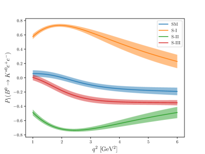
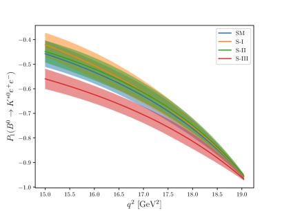
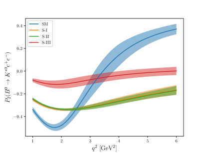
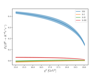
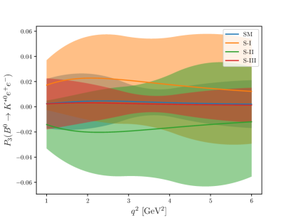
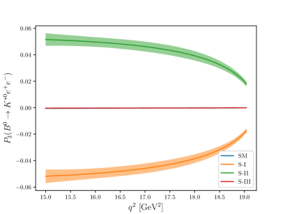
Figure 3: Plots of $P_{1,2,3}(q^{2})$ as a function of $q^{2}$ for the SM and three NP scenarios. The left and right panels correspond to the low ($[1.1,6.0]$ GeV²) and high ($[15,19]$ GeV²) $q^{2}$ bins, respectively.

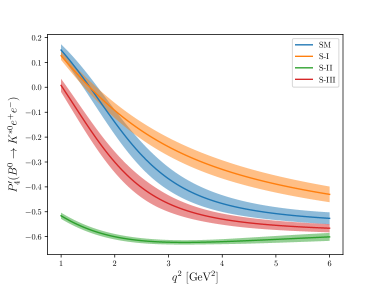
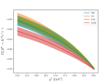
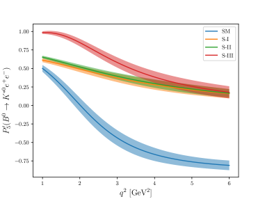
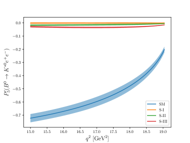
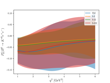
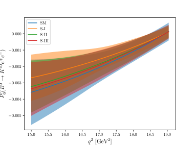
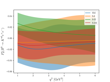
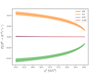
Figure 4: Plots of $P^{\prime}_{4,5,6,8}(q^{2})$ as a function of $q^{2}$ for the SM and three NP scenarios. The left and right panels correspond to the low ($[1.1,6.0]$ GeV²) and high ($[15,19]$ GeV²) $q^{2}$ bins respectively.

• The SM prediction of $P_{1}$ is suppressed in $1-6$ GeV². However the predicted values for three allowed NP solutions are large and distinct. The reason is following: The observable $P_{1}$ is very sensitive to the NP WCs $C^{\prime,e}_{9}$ and $C^{\prime,e}_{10}$. In the SM, these NP WCs vanish and this leads to a very small value of $P_{1}$. On the other hand, the three NP solutions have very large values of $C^{\prime,e}_{9}$ and $C^{\prime,e}_{10}$. Therefore any large values of these NP WCs can lead to a large deviation from the SM prediction. Hence $P_{1}$ in the low $q^{2}$ region can discriminate between all three NP solutions, particularly S-I and S-II. The sign of $P_{1}$ is opposite for these scenarios. Hence an accurate measurement of $P_{1}$ can distinguish between S-I and S-II solutions. In fact, measurement of $P_{1}$ with an absolute uncertainty of 0.05 can confirm or rule out S-I and S-II solutions by more than 4$\sigma$. In the high-$q^{2}$ region, the predictions for all allowed solutions are consistent with the SM.

• The observable $P_{2}$ can be a good discriminant of S-III provided we have handle over its $q^{2}$ distribution in $[1.1,6.0]$ GeV² bin. In this bin, $P_{2}(q^{2})$ has a zero crossing at $\sim 3.5$ GeV² for the SM prediction whereas there is no zero crossing for any of the allowed solutions. Scenarios S-I and S-II predict large negative values for $P_{2}$, around $-0.3$ whereas the S-III predicts relatively smaller negative values. Hence an accurate measurement of $q^{2}$ distribution of $P_{2}$ in $[1.1,6.0]$ GeV² bin can discriminate S-III with other two solutions. In high $q^{2}$ region, the predictions of $P_{2}$ for all three solutions are almost the same. These scenarios predict a large deviation from the SM. The SM prediction for $P_{2}$ is $\sim 0.4$ whereas all three solutions predict values closer to zero. Hence, an accurate measurement of the value of $P_{2}$ is a smoking-gun signal for the existence of NP in $b\to se^{+}e^{-}$ transition as the solution for the current $R_{K}$ and $R_{K^{*}}$ anomalies.

• The $P_{3}$ observable in the low-$q^{2}$ region cannot discriminate between the allowed solutions. However, in the high $q^{2}$ region, $P_{3}$ can uniquely discriminate the three solutions. In particular, the prediction of $P_{3}$ for S-III in the high $q^{2}$ is the same as the SM whereas the predictions for S-I and S-II are exactly equal and opposite.

• The $P^{\prime}_{4}$ in low-$q^{2}$ region can only distinguish S-II solution from the other two NP solutions and the SM. In high-$q^{2}$ region, it has a poor discrimination capability.

• In the low $q^{2}$ bin, $P^{\prime}_{5}$ has a zero crossing at $\sim 2$ GeV² and has an average negative value in the SM. For all three NP solutions, there is no zero crossing in $P^{\prime}_{5}$. Further, these scenarios predict a large positive values. In the high $q^{2}$ region, the SM predicts a large negative value of $P^{\prime}_{5}$ whereas NP scenarios predict values close to zero. Thus we see that if we impose the condition that NP in $b\to se^{+}e^{-}$ should simultaneously generate $R_{K}$ and $R_{K^{*}}$ within 1$\sigma$ of their measured values, it implies a large deviation in $P^{\prime}_{5}$ from the SM. This is reflected in the values of pull for the three allowed solutions which are relatively smaller than the other scenarios which fail to explain $R_{K}$ and $R_{K^{*}}$ simultaneously. The depletion in pull for these allowed solutions is due to inconsistency between the measured and predicted values of $P^{\prime}_{5}$.

• In the both low and high-$q^{2}$ regions, the NP predictions for $P^{\prime}_{6}$ for all three scenarios are consistent with the SM.

• The $P^{\prime}_{8}$ in the low-$q^{2}$ region does not have any discrimination capability. The predicted values for all solutions are consistent with the SM. In the high-$q^{2}$ region, both S-III and SM predict $P^{\prime}_{8}$ values close to zero whereas S-I and S-II predict large positive and negative values, respectively.

From this detailed study of the behavior of the optimized observables $P_{i}$, we find that both $P_{1}$ and $P_{4}^{\prime}$ at low-$q^{2}$ have the best capability to discriminate between all the three V/A solutions. The predicted values of $P_{1}$ are equal and opposite for S-I and S-II and of a much smaller magnitude for S-III. Moreover, each of the predicted values is appreciably different from the SM prediction. Their magnitudes are quite large $\sim(0.3-0.6)$ with a relative theoretical uncertainty of about $10\%$. Hence, a measurement of the variable $P_{1}$, with an experimental uncertainty of about $0.05$, will not not only confirm the presence of new physics in the $b\to se^{+}e^{-}$ amplitude but also can determine the correct WC of the NP operators. In the case $P_{4}^{\prime}$, the predictions of all the three solutions have the same sign but their magnitudes are quite different. The theoretical uncertainty in the predictions is quite low too. So, $P_{4}^{\prime}$ observable also has a good capability to distinguish between the three V/A solutions.

IV Conclusions

In this work, we intend to analyze $R_{K^{(*)}}$ anomalies by assuming NP only in $b\to se^{+}e^{-}$ decay. The effects of possible NP are encoded in the WCs of effective operators with different Lorentz structures. These WCs are constrained using all measurements in the $b\rightarrow se^{+}e^{-}$ sector along with lepton-universality-violating ratios $R_{K}/R_{K^{*}}$. We show that scalar/pseudoscalar NP operators and tensor NP operators can not explain the data in $b\to se^{+}e^{-}$ sector. We consider NP in the form of V/A operators, either one operator at a time or two similar operators at a time. We find that there are several scenarios which can provide a good fit to the data. However, there are only three solutions whose predictions of $R_{K}/R_{K^{*}}$, including $R_{K^{*}}$ in the in the low-$q^{2}$ bin ($0.045\,{\rm GeV}^{2}\leq q^{2}\leq 1.1{\rm GeV}^{2}$), match the data well. In order to discriminate between the three allowed V/A solutions, we consider several angular observables in the $B\to K^{*}e^{+}e^{-}$ decay. The three solutions predict very different values for the optimized observables $P_{1}$ and $P_{4}^{\prime}$ in the low-$q^{2}$ bin. Both these observables also have the additional advantage that the theoretical uncertainties in their predictions are less than $10\%$. Hence a measurement of either of these observables, to an absolute uncertainty of $0.05$, can lead to a unique identification of one of the solutions..

References

- (1) R. Aaij et al. [LHCb Collaboration], Phys. Rev. Lett. 113, 151601 (2014) [arXiv:1406.6482 [hep-ex]].
- (2) G. Hiller and F. Kruger, Phys. Rev. D 69, 074020 (2004) [hep-ph/0310219].
- (3) M. Bordone, G. Isidori and A. Pattori, Eur. Phys. J. C 76, no. 8, 440 (2016) [arXiv:1605.07633 [hep-ph]].
- (4) C. Bouchard et al. [HPQCD Collaboration], Phys. Rev. Lett. 111, no. 16, 162002 (2013) Erratum: [Phys. Rev. Lett. 112, no. 14, 149902 (2014)] [arXiv:1306.0434 [hep-ph]].
- (5) R. Aaij et al. [LHCb], Phys. Rev. Lett. 122 (2019) no.19, 191801 [arXiv:1903.09252 [hep-ex]].
- (6) R. Aaij et al. [LHCb], JHEP 08 (2017), 055 [arXiv:1705.05802 [hep-ex]].
- (7) A. Abdesselam et al. [Belle], [arXiv:1904.02440 [hep-ex]].
- (8) R. Aaij et al. [LHCb Collaboration], Phys. Rev. Lett. 111, 191801 (2013) [arXiv:1308.1707 [hep-ex]].
- (9) R. Aaij et al. [LHCb Collaboration], JHEP 1602, 104 (2016) [arXiv:1512.04442 [hep-ex]].
- (10) R. Aaij et al. [LHCb], Phys. Rev. Lett. 125 (2020) no.1, 011802 [arXiv:2003.04831 [hep-ex]].
- (11) R. Aaij et al. [LHCb Collaboration], JHEP 1509, 179 (2015) [arXiv:1506.08777 [hep-ex]].
- (12) M. Algueró, B. Capdevila, A. Crivellin, S. Descotes-Genon, P. Masjuan, J. Matias and J. Virto, Eur. Phys. J. C 79 (2019) no.8, 714 [arXiv:1903.09578 [hep-ph]].
- (13) A. K. Alok, A. Dighe, S. Gangal and D. Kumar, JHEP 1906, 089 (2019) [arXiv:1903.09617 [hep-ph]].
- (14) M. Ciuchini, A. M. Coutinho, M. Fedele, E. Franco, A. Paul, L. Silvestrini and M. Valli, Eur. Phys. J. C 79 (2019) no.8, 719 [arXiv:1903.09632 [hep-ph]].
- (15) G. D’Amico, M. Nardecchia, P. Panci, F. Sannino, A. Strumia, R. Torre and A. Urbano, JHEP 1709, 010 (2017) [arXiv:1704.05438 [hep-ph]].
- (16) J. Aebischer, W. Altmannshofer, D. Guadagnoli, M. Reboud, P. Stangl and D. M. Straub, Eur. Phys. J. C 80 (2020) no.3, 252 [arXiv:1903.10434 [hep-ph]].
- (17) K. Kowalska, D. Kumar and E. M. Sessolo, Eur. Phys. J. C 79, no. 10, 840 (2019) [arXiv:1903.10932 [hep-ph]].
- (18) A. Arbey, T. Hurth, F. Mahmoudi, D. M. Santos and S. Neshatpour, Phys. Rev. D 100, no. 1, 015045 (2019) [arXiv:1904.08399 [hep-ph]].
- (19) D. Kumar, J. Saini, S. Gangal and S. B. Das, Phys. Rev. D 97 (2018) no.3, 035007 [arXiv:1711.01989 [hep-ph]].
- (20) S. Kumbhakar and J. Saini, Eur. Phys. J. C 79 (2019) no.5, 394 [arXiv:1807.04055 [hep-ph]].
- (21) A. K. Alok, S. Kumbhakar and S. Uma Sankar, [arXiv:2001.04395 [hep-ph]].
- (22) F. Munir Bhutta, Z. R. Huang, C. D. Lü, M. A. Paracha and W. Wang, [arXiv:2009.03588 [hep-ph]].
- (23) G. Isidori, S. Nabeebaccus and R. Zwicky, [arXiv:2009.00929 [hep-ph]].
- (24) J. Kumar and D. London, Phys. Rev. D 99 (2019) no.7, 073008 [arXiv:1901.04516 [hep-ph]].
- (25) A. Datta, J. Kumar and D. London, Phys. Lett. B 797 (2019) 134858 [arXiv:1903.10086 [hep-ph]].
- (26) M. Ciuchini, M. Fedele, E. Franco, S. Mishima, A. Paul, L. Silvestrini and M. Valli, JHEP 06, 116 (2016) [arXiv:1512.07157 [hep-ph]].
- (27) T. Hurth, F. Mahmoudi and S. Neshatpour, Nucl. Phys. B 909, 737-777 (2016) [arXiv:1603.00865 [hep-ph]].
- (28) V. G. Chobanova, T. Hurth, F. Mahmoudi, D. Martinez Santos and S. Neshatpour, JHEP 07, 025 (2017) [arXiv:1702.02234 [hep-ph]].
- (29) T. Hurth, F. Mahmoudi and S. Neshatpour, [arXiv:2006.04213 [hep-ph]].
- (30) G. Hiller and M. Schmaltz, Phys. Rev. D 90 (2014), 054014 [arXiv:1408.1627 [hep-ph]].
- (31) D. Bardhan, P. Byakti and D. Ghosh, Phys. Lett. B 773, 505-512 (2017) [arXiv:1705.09305 [hep-ph]].
- (32) R. Aaij et al. [LHCb], Phys. Rev. Lett. 124 (2020) no.21, 211802 [arXiv:2003.03999 [hep-ex]].
- (33) R. Aaij et al. [LHCb], JHEP 05 (2013), 159 [arXiv:1304.3035 [hep-ex]].
- (34) R. Aaij et al. [LHCb], JHEP 04 (2015), 064 [arXiv:1501.03038 [hep-ex]].
- (35) J. P. Lees et al. [BaBar], Phys. Rev. Lett. 112 (2014), 211802 [arXiv:1312.5364 [hep-ex]].
- (36) R. Aaij et al. [LHCb], [arXiv:2010.06011 [hep-ex]].
- (37) S. Wehle et al. [Belle], Phys. Rev. Lett. 118 (2017) no.11, 111801 [arXiv:1612.05014 [hep-ex]].
- (38) D. M. Straub, [arXiv:1810.08132 [hep-ph]].
- (39) A. Bharucha, D. M. Straub and R. Zwicky, JHEP 08 (2016), 098 [arXiv:1503.05534 [hep-ph]].
- (40) N. Gubernari, A. Kokulu and D. van Dyk, JHEP 01 (2019), 150 [arXiv:1811.00983 [hep-ph]].
- (41) A. Khodjamirian, T. Mannel, A. A. Pivovarov and Y. M. Wang, JHEP 09 (2010), 089 [arXiv:1006.4945 [hep-ph]].
- (42) N. Gubernari, D. van Dyk and J. Virto, [arXiv:2011.09813 [hep-ph]].
- (43) F. James and M. Roos, “Minuit: A System for Function Minimization and Analysis of the Parameter Errors and Correlations”, Comput. Phys. Commun. 10 (1975), 343-367
- (44) F. James, “MINUIT Function Minimization and Error Analysis: Reference Manual Version 94.1”, CERN-D-506.
- (45) J. Heeck and W. Rodejohann, Phys. Rev. D 84 (2011), 075007 [arXiv:1107.5238 [hep-ph]].
- (46) W. Altmannshofer, S. Gori, M. Pospelov and I. Yavin, Phys. Rev. D 89 (2014), 095033 [arXiv:1403.1269 [hep-ph]].
- (47) A. Crivellin, G. D’Ambrosio and J. Heeck,Phys. Rev. Lett. 114 (2015), 151801 [arXiv:1501.00993 [hep-ph]].
- (48) W. Altmannshofer and I. Yavin, Phys. Rev. D 92 (2015) no.7, 075022 [arXiv:1508.07009 [hep-ph]].
- (49) A. Crivellin, J. Fuentes-Martin, A. Greljo and G. Isidori, Phys. Lett. B 766 (2017), 77-85 [arXiv:1611.02703 [hep-ph]].
- (50) C. Niehoff, P. Stangl and D. M. Straub, Phys. Lett. B 747 (2015), 182-186 [arXiv:1503.03865 [hep-ph]].
- (51) A. Datta, J. Kumar, J. Liao and D. Marfatia, Phys. Rev. D 97 (2018) no.11, 115038 [arXiv:1705.08423 [hep-ph]].
- (52) I. Doršner, S. Fajfer, A. Greljo, J. F. Kamenik and N. Košnik, Phys. Rept. 641 (2016), 1-68 [arXiv:1603.04993 [hep-ph]].
- (53) R. Aaij et al. [LHCb], JHEP 02 (2016), 104 [arXiv:1512.04442 [hep-ex]].
- (54) W. Altmannshofer, P. Ball, A. Bharucha, A. J. Buras, D. M. Straub and M. Wick, JHEP 01 (2009), 019 [arXiv:0811.1214 [hep-ph]].
- (55) S. Descotes-Genon, J. Matias, M. Ramon and J. Virto, JHEP 01 (2013), 048 [arXiv:1207.2753 [hep-ph]].
- (56) J. Gratrex, M. Hopfer and R. Zwicky, Phys. Rev. D 93 (2016) no.5, 054008 [arXiv:1506.03970 [hep-ph]].