Towards Better Accuracy-efficiency Trade-offs: Divide and Co-training

Abstract

The width of a neural network matters since increasing the width will necessarily increase the model capacity. However, the performance of a network does not improve linearly with the width and soon gets saturated. In this case, we argue that increasing the number of networks (ensemble) can achieve better accuracy-efficiency trade-offs than purely increasing the width. To prove it, one large network is divided into several small ones regarding its parameters and regularization components. Each of these small networks has a fraction of the original one’s parameters. We then train these small networks together and make them see various views of the same data to increase their diversity. During this co-training process, networks can also learn from each other. As a result, small networks can achieve better ensemble performance than the large one with few or no extra parameters or FLOPs, i.e., achieving better accuracy-efficiency trade-offs. Small networks can also achieve faster inference speed than the large one by concurrent running. All of the above shows that the number of networks is a new dimension of model scaling. We validate our argument with 8 different neural architectures on common benchmarks through extensive experiments. The code is available at https://github.com/FreeformRobotics/Divide-and-Co-training.

I Introduction

Increasing the width of neural networks to pursue better performance is common sense in network engineering [1, 2, 3]. However, the performance of networks does not improve linearly with the width. As shown in Figure 1, in the beginning, increasing width can gain promising improvement in accuracy; at a later stage, the improvement becomes slight and no longer matches the increasingly expensive cost. For example, EfficientNet baseline ($w=5.0$, width factor) gains less than $+0.5\%$ accuracy improvement compared to EfficientNet baseline ($w=3.8$) with nearly doubled FLOPs (floating-point operations). We call this the width saturation of a network. Increasing depth or resolution produces similar phenomena [1].

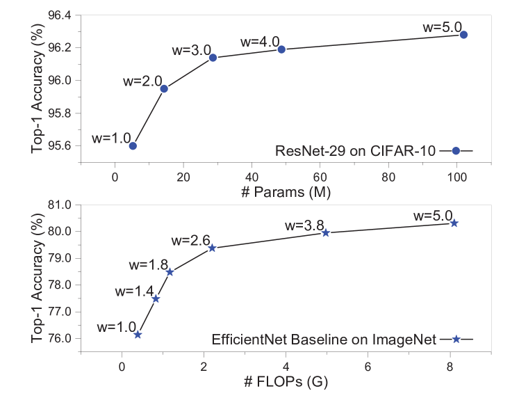
Figure 1: The width saturation of ResNeXt [3] and EfficientNet [1]. The gain does not match the expensive extra cost when the width ($w$) is large.

Besides the width saturation, we also observe that relatively small networks achieve close accuracies to very wide networks, i.e., ResNet-29 ($w=3.0$ v.s. $w=5.0$) and EfficientNet baseline ($w=2.6$ v.s. $w=5.0$) in Figure 1. In this case, an interesting question arises, can two small networks with a half width of a large one achieve or even surpass the performance of the latter? Firstly, ensemble is a practical technique and can improve the generalization performance of individual neural networks [4, 5, 6, 7, 8]. Kondratyuk et al. [9] already demonstrate that the ensemble of several smaller networks is more efficient than a large model in some cases. Secondly, multiple networks can collaborate with their peers and learning from each other during training to achieve better individual or ensemble performance. This is verified by some deep mutual learning [10, 11, 12] and co-training [13] works.

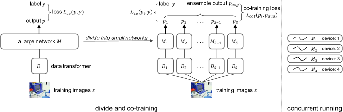
Figure 2: Left: divide one large network into several small ones and co-train. Right: concurrent running of small networks on different devices during inference.

Based on the above analysis, we argue that increasing the number of networks (ensemble) can achieve better accuracy-efficiency trade-offs than purely increasing the width. A straightforward demonstration is given in this work: we divide one large network into several pieces and show that these small networks can achieve better ensemble performance than the large one with almost the same computation costs.

The overall framework is shown in Figure 2. 1) dividing: Given one large network, we first divide the network according to its width, more precisely, the parameters or FLOPs of the network. For instance, if we want to divide a network into two small networks, the number of the small one’s parameters will become half of the original. During this division process, the regularization components will also be changed as the model capacity degrades. Particularly, weight decay and drop layers will be divided accordingly with the network width. 2) co-training: After dividing, small networks are trained with different views of the same data [13] to increase the diversity of networks and achieve better ensemble performance [5]. This is implemented by applying different data augmentation transformers in practice. At the same time, small networks can also learn from each other [10, 13, 12] to further boost individual performance. Thus we add Jensen-Shannon divergence among all predictions, i.e., co-training loss in Figure 2. In this way, one network can learn valuable knowledge about intrinsic object structure information from predicted posterior probability distributions of its peers [14]. 3) concurrent running: Small networks can also achieve faster inference speed than the original one through concurrent running on different devices when resources are sufficient. Some different networks and their average latency (inference speed) on ImageNet [15] are shown in Figure 3.

We conduct extensive experiments with dividing and co-training strategies for 8 different networks. Generally, small networks after dividing accomplish better ensemble performance than the original big network with similar parameters and FLOPs, i.e., better accuracy-efficiency trade-offs are achieved. We also reach competitive accuracy with state-of-the-art methods, specifically, 98.31% on CIFAR-10 [16], 89.46% on CIFAR-100, and 83.60% on ImageNet [15]. Furthermore, we validate our method for object detection and demonstrate the generality of dividing and ensemble. All evidence suggests that people should consider the number of networks as a meaningful dimension of network engineering besides commonly known width, depth, and resolution.

Our contributions are summarized as follows:

• We post the claim that increasing the number of networks can achieve better accuracy-efficiency trade-offs than purely increasing the network width.

• We propose novel dividing strategies for 8 different networks regarding their parameters and regularizations to achieve better performance with similar costs.

• Practical co-training techniques are developed to help small networks learn from their peers.

• We provide best practices and instructive conclusions for dividing and co-training via extensive experiments and thorough ablations on classification and object detection.

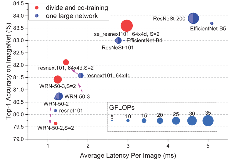
Figure 3: Networks and their inference latency. $S$ is the number of networks. Test on Tesla V100(s) with mixed precision [17] and batch size 100.

II Related works

Neural network architecture design

Since the success of AlexNet [18] on ImageNet [15], deep learning methods dominate the field of computer vision, and network engineering becomes a core topic. Many excellent architectures emerged, e.g., NIN [19], VGG [20], Inception [21], ResNet [22], Xception [23]. They explored different ways to design an effective and efficient model, e.g., $1\times 1$ convolution kernels, stacked convolution layers with small kernels, combination of different convolution and pooling operations, residual connection, depthwise separable convolution. In recent years, neural architecture search (NAS) becomes more and more popular. People hope to automatically learn or search for the best neural architectures for certain tasks with machine learning methods. We name a few here, reinforcement learning based NAS [24], progressive neural architecture search (PNASNet [25]), differentiable architecture search (DARTS [26]), etc.

Implicit ensemble methods

Ensemble methods use multiple learning algorithms to obtain better performance than any of them. Some layer splitting methods [21, 3, 27] adopt an implicitly ”divide and ensemble” strategy, namely, they divide a single layer in a model and then fuse their outputs to get better performance. Dropout [28] can also be interpreted as an implicit ensemble of multiple sub-networks within one full network. Slimmable Network [29, 30] derives several networks with different widths from a full network and trains them in a parameter-sharing way to achieve adaptive accuracy-efficiency trade-offs at runtime. MutualNet [11] further trains these sub-networks mutually to make the full network achieve better performance. These methods get several dependent models after implicitly splitting, while our methods obtain independent models in terms of parameters after dividing. They are also compatible with our methods and can be applied to any single model in our system.

Collaborative learning

Collaborative learning refers to a variety of educational approaches involving the joint intellectual effort by students, or students and teachers together [31]. It was formally introduced in deep learning by [32], which was used to describe the simultaneous training of multiple classifier heads of a network. Actually, according to its original definition, many works involving two or more models learning together can also be called collaborative learning, e.g., DML [12], co-training [33, 13], mutual mean-teaching (MMT) [10], cooperative learning [34], knowledge distillation [14]. Their core idea is similar, i.e., enhancing the performance of one or all models by training them with some peers or teachers. They inspire our co-training algorithm.

III Method

First of all, we recall the common framework of deep image classification. Given a neural model $M$ and $N$ training samples $\mathcal{X}=\{\bm{x}_{n}\}_{n=1}^{N}$ from $C$ classes, the objective is cross entropy:

$$\mathcal{L}_{ce}(p,y)=-\frac{1}{N}\sum_{n=1}^{N}\sum_{c=1}^{C}y_{n,c}\log(p_{n,c}),$$ (1)

where $y\in\{0,1\}$ is the ground truth label and $p\in[0,1]$ is the softmax normalized probability given by $M$.

III-A Division

Parameters

In Figure 2, we divide one large network $M$ into $S$ small networks $\{M_{1},M_{2},\ldots,M_{S}\}$. The principle is keeping the metrics — the number of parameters or FLOPs roughly unchanged before and after dividing. $M$ is usually a stack of convolutional (conv.) layers. Following the definition in PyTorch [35], its kernel size is $K\times K$, numbers of channels of input and output feature maps are $C_{in}$ and $C_{out}$, and the number of groups is $d$, which means every $\frac{C_{in}}{d}$ input channels are convolved with its own sets of filters, of size $\frac{C_{out}}{d}$. In this case, the number of parameters and FLOPs are:

$$\text{Params}:~{} K^{2}\times\frac{C_{in}}{d}\times\frac{C_{out}}{d}\times d,$$ (2)

$$\text{FLOPs}:~{} (2\times K^{2}\times\frac{C_{in}}{d}-1)\times H\times W\times C_{out},$$ (3)

where $H\times W$ is the size of the output feature map and $-1$ occurs because the addition of $\frac{C_{in}}{d}\times K^{2}$ numbers only needs $(\frac{C_{in}}{d}\times K^{2}-1)$ times operations. The bias is omitted for the sake of brevity. For depthwise convolution [36], $d=C_{in}$.

Generally, $C_{out}=t_{1}\times C_{in}$, where $t_{1}$ is a constant. Therefore, if we want to divide a conv. layer by a factor $S$, we just need to divide $C_{in}$ by $\sqrt{S}$:

$$\frac{K^{2}\times C_{in}\times C_{out}}{S}\times\frac{1}{d}=K^{2}\times t_{1}\times(\frac{C_{in}}{\sqrt{S}})^{2}\times\frac{1}{d}.$$ (4)

For instance, if we divide a bottleneck $\Big{[}\begin{smallmatrix}1\times 1,&64\\ 3\times 3,&64\\ 1\times 1,&256\end{smallmatrix}\Big{]}$ in ResNet by 4, it becomes 4 small blocks $\Big{[}\begin{smallmatrix}1\times 1,&32\\ 3\times 3,&32\\ 1\times 1,&128\end{smallmatrix}\Big{]}$. Each small block has a quarter of the parameters or FLOPs of the original block.

In practice, the numbers of output channels have the greatest common divisor (GCD). The GCD of most ResNet variants [22, 2, 3, 37] is the $C_{out}$ of the first convolutional layer. For other networks, like EfficientNet [1], their GCD is a multiple of 8 or some other numbers. In general, when we want to divide a network by $S$, we just need to find its GCD, and replace it with GCD$/\sqrt{S}$, then it is done.

For networks mainly consisted of group convolutions like ResNeXt [3], we keep $\frac{C_{in}}{d}$ fixed, i.e., $C_{in}=t_{2}\times d$, where $t_{2}$ is a constant. Namely, the number of channels per group is unchanged during dividing, and the number of groups will be divided. We substitute the $C_{in}$ in Eq. (4) with the above equation and get:

$$K^{2}\times t_{1}\times t_{2}^{2}\times\frac{d}{S}.$$ (5)

Then the division can be easily achieved by dividing $d$ by $S$. This way is more concise than the square root operations.

For networks that have a constant global factor linearly related to the channel number, we simply divide the factor by $\sqrt{S}$, e.g., the widen factor of WRN [2], the growth rate of DenseNet [38], and the additional rate of PyramidNet [39].

Regularization

After dividing, the model capacity degrades and the regularization components in networks should change accordingly. Under the assumption that the model capacity is linearly dependent with the network width, we change the magnitude of dropping regularization linearly. Specifically, the dropping probabilities of dropout [28], ShakeDrop [40], and stochastic depth [41] are divided by $\sqrt{S}$ in our experiments. As for weight decay [42], it is a little complex as its intrinsic mechanism is still vague [43, 44]. We test some dividing manners and adopt two dividing strategies — no dividing and exponential dividing in this paper:

$$wd^{\star}=wd\times\exp(\frac{1}{S}-1.0),$$ (6)

where $wd$ is the original weight decay value and $wd^{\star}$ is the new value after dividing. No dividing means the weight decay value keeps unchanged. The above two dividing strategies are empirical criteria. In practice, the best way now is trial and error. Besides, we adopt exponential dividing rather than directly dividing the $wd$ by $\sqrt{S}$ because the latter may lead to too small weight decay values to maintain the generalization performance when $S$ is large.

The above dividing mechanism is usually not perfect, i.e., the number of parameters of $M_{i}$ may not be exactly $1/S$ of $M$. Firstly, $\sqrt{S}$ may not be an integer. In this case, we round ${C_{in}}/{\sqrt{S}}$ in Eq. (4) to a nearby even number. Secondly, the division of the first layer and the last fully-connected layer is not perfect because the input channel (color channels) and output channel (number of object classes) are fixed.

Concurrent running

Small networks can also achieve faster inference speed than the large network by concurrent running on different devices as shown in Figure 2. Typically, a device is an NVIDIA GPU. Theoretically, if one GPU has enough processing units, e.g., streaming multiprocessor, small networks can also run concurrently within one GPU with multiple CUDA Streams [45]. However, we find this is impractical on a Tesla V100 GPU in experiments. One small network is already able to occupy most of the computational resources, and different networks can only run in sequence. Therefore, we only discuss the multiple devices fashion.

III-B Co-training

The generalization error of neural network ensemble (NNE) can be interpreted as Bias-Variance-Covariance Trade-off [6, 7]. Let $f$ be the function model learned, $g(\bm{x})$ be the target function, and $f_{en}(\bm{x};\mathcal{X})=\frac{1}{S}\sum_{i=1}^{S}f_{i}(\bm{x};\mathcal{X})$. Then the expected mean-squared ensemble error is:

$$\mathbb{E}_{\mathcal{X}}[\big{(}f_{en}(\bm{x};\mathcal{X})-g(\bm{x})\big{)}^{2}]=\big{(}\mathbb{E}_{\mathcal{X}}[f_{en}(\bm{x})-g(\bm{x})]\big{)}^{2}$$

$$+\mathbb{E}_{\mathcal{X}}\big{[}\frac{1}{S^{2}}\sum\nolimits_{i=1}^{S}\big{(}f_{i}(\bm{x};\mathcal{X})-\mathbb{E}_{\mathcal{X}}[f_{i}(\bm{x};\mathcal{X})]\big{)}^{2}\big{]}$$

$$+\mathbb{E}_{\mathcal{X}}\big{[}\frac{1}{S^{2}}\sum\nolimits_{i=1}^{S}\sum\nolimits_{j\neq i}^{S}\big{(}f_{i}(\bm{x};\mathcal{X})-\mathbb{E}_{\mathcal{X}}[f_{i}(\bm{x};\mathcal{X})]\big{)}$$

$$\times\big{(}f_{j}(\bm{x};\mathcal{X})-\mathbb{E}_{\mathcal{X}}[f_{j}(\bm{x};\mathcal{X})]\big{)}\big{]},~{}$$ (7)

where the first term is the square bias ($\operatorname{\textit{Bias}}^{2}$) of the combined system, the second and third terms are the variance ($\operatorname{\textit{Var}}$) and covariance ($\operatorname{\textit{Cov}}$) of the outputs of individual networks. A clean form is $\mathbb{E}[\frac{1}{S}\operatorname{\textit{Var}}+(1-\frac{1}{S})\operatorname{\textit{Cov}}+\operatorname{\textit{Bias}}^{2}]$. Data noise is omitted here. The detailed proof is given by Ueda et al. [46].

Different initialization and data views

Increasing the diversity of networks without increasing $\operatorname{\textit{Var}}$ or $\operatorname{\textit{Bias}}$ can decrease the correlation ($\operatorname{\textit{Cov}}$) between networks. To this end, small networks are initialized with different weights [5]. Then, when feeding the training data, we apply different data transformers $D_{i}$ on the same data for different networks as shown in Figure 2. In this way, $\{M_{1},M_{2},\ldots,M_{S}\}$ are trained on different views $\{D_{1}(\bm{x}),D_{2}(\bm{x}),\ldots,D_{S}(\bm{x})\}$ of $\bm{x}$. In practice, different data views are generated by the randomness of data augmentation. Besides the commonly used random resize, random crop, and random flip, we introduce random erasing [47] and AutoAugment [48] policies. AutoAugment has 14 image transformation operations, e.g., shear, translate, rotate, and auto contrast. It searches tens of different policies which are consisted of two operations and randomly chooses one policy during the data augmentation process. By applying these random data augmentations, we can guarantee that $D_{i}(\bm{x})$ produces different views of $\bm{x}$ across multiple runs.

Co-training loss

Knowledge distillation and DML [12] show that one network can boost its performance by learning from a teacher or cohorts. Namely, a deep ensemble system can reduce its $\operatorname{\textit{Bias}}$ in this way. Besides, following the co-training assumption [33], small networks are expected to have consistent predictions on $\bm{x}$ although they see different views of $\bm{x}$. From the perspective of Eq. (7), this can reduce the variance of networks and avoid poor performance caused by overly decorrelated networks [7]. Therefore, we adopt Jensen-Shannon (JS) divergence among predicted probabilities as the co-training objective [13] :

$$\mathcal{L}_{cot}(p_{1},p_{2},\ldots,p_{S})=H(\frac{1}{S}\sum_{i=1}^{S}p_{i})-\frac{1}{S}\sum_{i=1}^{S}H(p_{i}),$$ (8)

where $p_{i}$ is the estimated probability of $M_{i}$, and $H(p)=\mathbb{E}[-\log(p)]$ is the Shannon entropy of the distribution of $p$. Through this co-training manner, one network can learn valuable information from its peers, which defines a rich similarity structure over objects. For example, a model classifies an object as Chihuahua may also give high confidence about Japanese spaniel since they are both dogs [14]. DML uses the Kullback-Leibler (KL) divergence between predictions of every two networks. Their purpose is similar to ours.

The overall objective function is a combination of the classification losses of small networks and the co-training loss:

$$\mathcal{L}_{all}=\sum_{i=1}^{S}\mathcal{L}_{ce}(p_{i},y)+\lambda_{cot}\mathcal{L}_{cot}(p_{1},p_{2},\ldots,p_{S}),$$ (9)

where $\lambda_{cot}=0.5$ is a weight factor of $\mathcal{L}_{cot}(\cdot)$ and it is chosen by cross-validation. At the early stage of training, the outputs of networks are full of randomness, so we adopt a warm-up scheme for $\lambda_{cot}$ [49, 13]. Specifically, we use a linear scaling up strategy when the current training epoch is less than a certain number — 40 and 60 for CIFAR and ImageNet, respectively. $\lambda_{cot}=0.5$ is also an equilibrium point between learning diverse networks and producing consistent predictions. During inference, we average the outputs before softmax layers as the final ensemble output.

IV Experiment

IV-A Experimental setup

Datasets  We adopt CIFAR-10, CIFAR-100 [16], and ImageNet 2012 [15] datasets. CIFAR-10 and CIFAR-100 contain 50K training and 10K test RGB images of size 32$\times$32, labeled with 10 and 100 classes, respectively. ImageNet 2012 contains 1.28 million training images and 50K validation images from 1000 classes. For CIFAR and ImageNet, crop size is 32 and 224, batch size is 128 and 256, respectively.

Learning rate and training epochs  We apply warm up and cosine learning rate policy [50, 51]. If the initial learning rate is $lr$ and current epoch is $epoch$, for the first slow_epoch steps, the learning rate is $lr\times\frac{\textit{epoch}}{\textit{slow\_epoch}}$; for the rest epochs, the learning rate is $0.5\times lr\times(1+\cos(\pi\times\frac{\textit{epoch}-\textit{slow\_epochs}}{\textit{max\_epoch}-\textit{slow\_epoch}}))$. Generally, $lr$ is 0.1; $\{\textit{max\_epoch},\textit{slow\_epoch}\}$ is {300, 20} and {120, 5} for CIFAR and ImageNet, respectively. Models before and after dividing are trained for the same epochs.

TABLE I: Influence of various experiment settings on CIFAR-100. step-lr means step learning rate policy [22]. When the erasing probability $p_{e}=1.0$, random erasing acts like cutout [52].

Method	step-lr	cos-lr	rand. erasing	mixup	AutoAug.	Top-1 err. (%)
ResNet-110 [53] original: 26.88%	✓					24.71 $\pm$ 0.22
		✓				24.15 $\pm$ 0.07
		✓	✓, $p_{e}=1.0$			23.43 $\pm$ 0.01
		✓	✓, $p_{e}=0.5$			23.11 $\pm$ 0.29
		✓	✓, $p_{e}=0.5$	✓, $\lambda=0.2$		21.22 $\pm$ 0.28
		✓	✓, $p_{e}=0.5$	✓, $\lambda=0.2$	✓	19.19 $\pm$ 0.23

Data augmentation  Random crop and resize, random left-right flipping, AutoAugment [48], random erasing [47], and mixup [54] are used during training. Label smoothing [55] is only applied when training on ImageNet.

Weight decay  Generally, weight decay is 1e-4. For {EfficientNet-B3, ResNeXt-29, WRN-28-10, WRN-40-10} on CIFAR datasets, it is 5e-4. Bias and parameters of batch normalization [56] are left undecayed.

Besides, we use kaiming weight initialization [57]. The optimizer is nesterov [58] accelerated SGD with a momentum 0.9. ResNet variants adopt the modifications introduced in [51], i.e., replacing the first $7\times 7$ conv. with three consecutive $3\times 3$ conv. and put an $2\times 2$ average pooling layer before $1\times 1$ conv. when there is a need to downsample. The code is implemented in PyTorch [35]. Influence of some settings is shown in Table I.

TABLE II: Results of Top-1 error (%) on CIFAR-100. The last three rows are trained for 1800 epochs. $S$ is the number of small networks after dividing. Train from scratch, no extra data. Weight decay value keeps unchanged except {WRN-40-10, 1800 epochs}, which applies Eq. (6). The maximal reduction of error of different networks is shown in blue.

	original	re-implementation			(# Networks) $\bm{S=2}$			(# Networks) $\bm{S=4}$
Method	error	error	MParams	GFLOPs	error	MParams	GFLOPs	error	MParams	GFLOPs
ResNet-110 [53]	26.88	18.96	1.17	0.17	18.32${}_{(0.64~{}\downarrow)}$	1.33	0.20	19.56${}_{(0.63~{}\uparrow)}$	1.21	0.18
ResNet-164 [53]	24.33	18.38	1.73	0.25	17.12${}_{(1.26~{}\downarrow)}$	1.96	0.29	18.05${}_{(0.33~{}\downarrow)}$	1.78	0.26
SE-ResNet-110 [37]	23.85	17.91	1.69	0.17	17.37${}_{(0.54~{}\downarrow)}$	1.89	0.20	18.33${}_{(0.42~{}\uparrow)}$	1.70	0.18
SE-ResNet-164 [37]	21.31	17.37	2.51	0.26	16.31${}_{(1.06~{}\downarrow)}$	2.81	0.29	17.21${}_{(0.16~{}\downarrow)}$	2.53	0.27
EfficientNet-B0 [1]†	-	18.50	4.13	0.23	18.20${}_{(0.30~{}\downarrow)}$	4.28	0.24	17.85${}_{(0.65~{}\downarrow)}$	4.52	0.30
EfficientNet-B3 [1]†	-	18.10	10.9	0.60	17.00${}_{(1.10~{}\downarrow)}$	11.1	0.60	16.62${}_{(1.48~{}\downarrow)}$	11.7	0.65
WRN-16-8 [2]	20.43	18.69	11.0	1.55	17.37${}_{(1.32~{}\downarrow)}$	12.4	1.75	17.07${}_{(1.62~{}\downarrow)}$	11.1	1.58
ResNeXt-29, 8$\times$64d [3]	17.77	16.43	34.5	5.41	14.99${}_{(1.44~{}\downarrow)}$	35.4	5.50	14.88${}_{(1.55~{}\downarrow)}$	36.9	5.67
WRN-28-10 [2]	19.25	15.50	36.5	5.25	14.48${}_{(1.02~{}\downarrow)}$	35.8	5.16	14.26${}_{(1.24~{}\downarrow)}$	36.7	5.28
WRN-40-10 [2]	18.30	15.56	55.9	8.08	14.28${}_{(1.28~{}\downarrow)}$	54.8	7.94	13.96${}_{(1.60~{}\downarrow)}$	56.0	8.12
DenseNet-BC-190 [38]	17.18	14.10	25.8	9.39	12.64${}_{(1.46~{}\downarrow)}$	25.5	9.24	12.56${}_{(1.54~{}\downarrow)}$♯	26.3	9.48
PyramidNet-272 [39]+ShakeDrop [40]	14.96	11.02	26.8	4.55	10.75${}_{(0.27~{}\downarrow)}$	28.9	5.24	10.54${}_{(0.48~{}\downarrow)}$♯	32.8	6.33
WRN-40-10 [2]	18.30	16.02	55.9	8.08	14.09${}_{(1.93~{}\downarrow)}$	54.8	7.94	13.10${}_{(2.92~{}\downarrow)}$♯	56.0	8.12

• When training on CIFAR-100, the stride of EfficientNet at the stage 4&7 is set to be 1. Original EfficientNet on CIFAR-100 is pre-trained while we train it from scratch.

• These results rank #2, #6, and #7 on public leaderboard paperswithcode.com/sota/image-classification-on-cifar-100 (without extra training data) at the time of submission.

IV-B Results on CIFAR and ImageNet dataset

IV-B1 CIFAR-100

In Table II, dividing and co-training achieve consistent improvements with similar or even fewer parameters or FLOPs. Additional cost occurs because the division of a network is not perfect, as mentioned in Sec. III-A. Three conclusions can be drawn from these results 7 networks.

Conclusion 1

Increasing the number, width, and depth of networks together is more efficient and effective than purely increasing the width or depth.

For all networks in Table II, dividing and co-training gain promising improvement. We also notice, ResNet-110 ($S=2$) $>$ ResNet-164, SE-ResNet-110 ($S=2$) $>$ SE-ResNet-164, EfficientNet-B0 ($S=4$) $>$ EfficientNet-B3, and WRN-28-10 ($S=4$) $>$ WRN-40-10 with fewer parameters, where $>$ means the former has better performance. By contrast, the latter is deeper or wider. Besides, with wider or deeper networks, dividing and co-training can gain more improvement, e.g., ResNet-110 (+0.64) vs. ResNet-164 (+1.26), SE-ResNet-110 (+0.54) vs. SE-ResNet-164 (+1.06), WRN-28-10 (+1.24) vs. WRN-40-10 (+1.60), and EfficientNet-B0 (+0.65) vs. EfficientNet-B3 (+1.48). All of the above demonstrates the superiority of increasing the number of networks. It is also clear that increasing the number, width, and depth of networks together is a better choice than purely scaling up one single dimension during model engineering.

Conclusion 2

The ensemble performance is closely related to individual performance.

The relationship between the average accuracy and ensemble accuracy is shown in Figure 4. When calculating the average accuracy, we separately calculate the accuracies of small networks and average them. From the big picture, the average accuracy is positively correlated with the ensemble accuracy. The higher the average accuracy, the better the ensemble performance. This coincides with the Eq. (7) because the stronger the individual networks the smaller the $\operatorname{\textit{Bias}}$.

At the same time, we note that there is a big gap between the average accuracy and ensemble accuracy. The ensemble accuracy is higher than the average accuracy by a large margin. This gap may be filled by two factors according to Eq. (7): the decayed variance of individual networks and learned diverse networks during the co-training process.

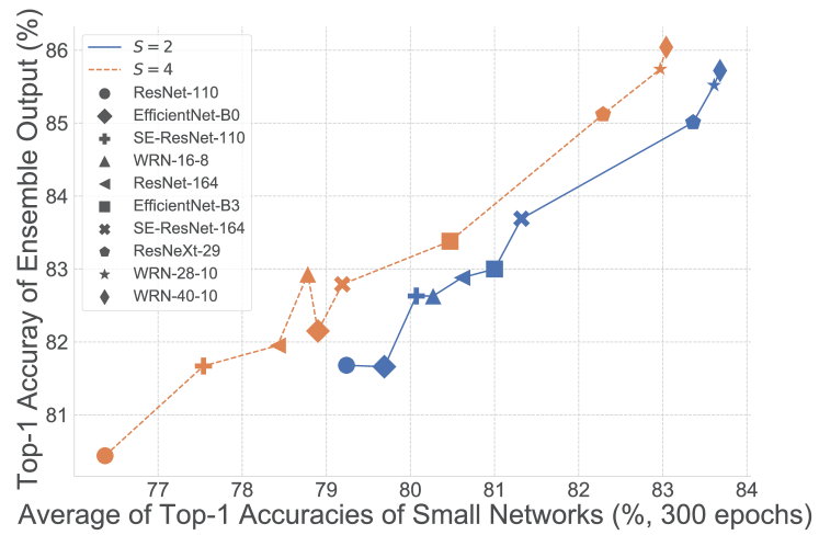
Figure 4: The relationship between the numerical average of accuracies and ensemble accuracy of small networks on CIFAR-100.

Conclusion 3

A necessary width/depth of networks matters.

In Table II, ResNet-110 ($S=4$) and SE-ResNet-110 ($S=4$) get a drop in performance, 0.63%$\downarrow$ and 0.42%$\downarrow$, respectively. In Figure 4, these two networks obtain the first two lowest average accuracies. If we take one step further to look at the architecture of these small networks, we will find they have input channels $[8,16,32]$ at the first layer of their three blocks. These networks are too thin compared to the original one with $[16,32,64]$ channels. In this case, the magnitude of the decayed variance of individual networks is smaller than the magnitude of gained accuracy (decayed bias) from increasing the channels (width) of a single network. Consequently, individual networks cannot gain satisfying accuracy and lead to inferior ensemble performance as conclusion 2 said. This demonstrates that a necessary width is essential. The conclusion also applies to PyramidNet-272, which gets a relatively slight improvement with dividing and co-training as its base channel is small, i.e., 16. Increasing the width of networks is still effective when the width is very small.

TABLE III: Results of Top-1 error (%) on CIFAR-10. $S$ is the number of small networks after dividing. Divide weight decay as Eq. (6). No extra data and train from scratch. Methods compared here are AutoAugment [48], RandAugment [59], Fixup-init [60], Cutout [52], Mixup [54], ShakeDrop [40], and Fast AutoAugment [61].

Method	error		MParams	GFLOPs
ResNet-164 [53]	5.46		1.73	0.25
SE-ResNet-164 [37]	4.39		2.51	0.26
WRN-28-10 [2]	4.00		36.5	5.25
ResNeXt-29, 8$\times$64d [3]	3.65		34.5	5.41
WRN-28-10 [2, 48]	2.68		36.5	5.25
WRN-28-10 [2, 59]	2.70		36.5	5.25
WRN-40-10 [2, 60, 54, 52]	2.30		55.9	8.08
Shake-Shake 26 2$\times$96d [62, 48]	2.00		26.2	3.78
Shake-Shake 26 2$\times$96d [62, 59]	2.00		26.2	3.78
PyramidNet-272 [39, 40, 61]	1.70		26.2	4.55
	epochs
re-implementation	300	1800	MParams	GFLOPs
SE-ResNet-164	2.98	2.19	2.49	0.26
ResNeXt-29, 8$\times$64d	2.69	2.23	34.4	5.40
WRN-28-10	2.28	2.41	36.5	5.25
WRN-40-10	2.33	2.19	55.8	8.08
Shake-Shake 26 2$\times$96d		2.00	26.2	3.78
SE-ResNet-164, $S=2$	2.84	2.20	2.81	0.29
ResNeXt-29, 8$\times$64d, $S=2$	2.12	1.94	35.1	5.49
WRN-28-10, $S=2$	2.06	1.81	35.8	5.16
WRN-28-10, $S=4$	2.01	1.68♯	36.5	5.28
WRN-40-10, $S=4$	2.01	1.62♯	55.9	8.12
Shake-Shake 26 2$\times$96d, $S=2$		1.75	23.3	3.38
Shake-Shake 26 2$\times$96d, $S=4$		1.69♯	26.3	3.82

• These results rank #6, #7, and #8 on public leaderboard paperswithcode.com/sota/image-classification-on-cifar-10 (without extra training data) at the time of submission.

In Table II, ResNet-164 ($S=4$) and SE-ResNet-164 ($S=4$) still get improvements, although their performance is not as good as applying ($S=2$). In Figure 4, small networks of ResNet-164 and SE-ResNet-164 with ($S=4$) also get better performance than ResNet-110 and SE-ResNet-110 with ($S=4$), respectively. This reveals that a necessary depth can help guarantee the model capacity and achieve better ensemble performance. In a word, after dividing, the small networks should maintain a necessary width or depth to guarantee their model capacity and achieve satisfying ensemble performance. This is consistent with some previous works. Kondratyuk et al. [9] show that the ensemble of some small models with limited depths and widths cannot achieve promising ensemble performance compared to some large models.

From conclusion 1 – 3, we can learn some best practices about effective model scaling. When the width/depth of networks is small, increasing width/depth can still get substantial improvement. However, when width or depth becomes large and increasing them yields little gain (Figure 1), it is more effective to increase the number of networks. This comes to our core conclusion — Increasing the number, width, and depth of networks together is more efficient and effective than purely scaling up one dimension of them.

IV-B2 CIFAR-10

Results on the CIFAR-10 are shown in Table III. Although the Top-1 accuracy on CIFAR-10 is already very high, dividing and co-training can also achieve significant improvement. It is worth noting {WRN-28-10, epoch 1800} gets worse performance than {WRN-28-10, epoch 300}, namely, WRN-28-10 may overfit on CIFAR-10 when trained for more epochs. In contrast, dividing and co-training can help WRN-28-10 get consistent improvement with increasing training epochs. This is because we can learn diverse networks from the data. In this way, even if one model overfits, the ensemble of different models can also make a comprehensive and correct prediction. From the perspective of Eq. (7), diverse networks reduce the $\operatorname{\textit{Var}}$ or achieve a negative $\operatorname{\textit{Cov}}$. The conclusion also applies to {WRN-40-10, 300 epochs} and {WRN-40-10, 1800 epochs} on CIFAR-100. This shows ensembles of neural networks are not only more accurate but also more robust than individual networks.

TABLE IV: Single crop results on ImageNet 2012 validation set. No extra data and train from scratch. $S$ is the number of small networks after dividing. Acc. of $M_{i}$ is the accuracy of small networks. Only WRN applies Eq. (6); others keep weight decay unchanged.

Method	Top-1 / Top-5 Acc.	MParams / GFLOPs	Crop / Batch / Epochs	Acc. of $M_{i}$
WRN-50-2 [2]	78.10   /   93.97	68.9   /   12.8	224  /  256  / 120	—
ResNeXt-101, 64$\times$4d [3]	79.60   /   94.70	83.6   /   16.9	224  /  256  / 120
ResNet-200 + AutoAugment [48]	80.00   /   95.00	64.8   /   16.4	224  / 4096 / 270
SENet-154 [37]	82.72   /   96.21	115.0  /   42.3	320  / 1024 / 100
SENet-154 + MultiGrain [63]	83.10   /   96.50	115.0  /   83.1	450  /  512  / 120
PNASNet-5 $(N=4,F=216)$ [25]†	82.90   /   96.20	86.1   /   25.0	331  / 1600 / 312
AmoebaNet-C $(N=6,F=228)$ [64]†	83.10   /   96.30	155.3  /   41.1	331  / 3200 / 100
ResNeSt-200 [27]	83.88   /     —	70.4   /   35.6	320  / 2048 / 270
EfficientNet-B6 [1]	84.20   /   96.80	43.0   /   19.0	528  / 4096 / 350
EfficientNet-B7 [1]	84.40   /   97.10	66.7   /   37.0	600  / 4096 / 350
WRN-50-2 (re_impl.)	80.66   /   95.16	68.9   /   12.8	224  /  256  / 120	—
WRN-50-3 (re_impl.)	80.74   /   95.40	135.0  /   23.8	224  /  256  / 120
ResNeXt-101, 64$\times$4d (re_impl.)	81.57   /   95.73	83.6   /   16.9	224  /  256  / 120
EfficientNet-B7 (re_impl.)♯	81.83   /   95.78	66.7   /   10.6	320  /  256  / 120
WRN-50-2, $S=2$	79.64   /   94.82	51.4   /   10.9	224  /  256  / 120	78.68, 78.66
WRN-50-3, $S=2$	81.42   /   95.62	138.0  /   25.6	224  /  256  / 120	80.32, 80.24
ResNeXt-101, 64$\times$4d, $S=2$	82.13   /   95.98	88.6   /   18.8	224  /  256  / 120	81.09, 81.02
EfficientNet-B7, $S=2$	82.74   /   96.30	68.2   /   10.5	320  /  256  / 120	81.39, 81.83
EfficientNet-B7, $S=4$	82.75   /   96.22	70.9   /   12.6	320  /  256  / 120	80.49, 80.55, 80.56, 80.48
SE-ResNeXt-101, 64$\times$4d, $S=2$	83.60   /   96.69	98.0   /   38.2	320  /  128  / 350	82.43, 82.46

• PNASNet and AmoebaNet use 100 P100 workers. On each worker, batch size is 16 or 32.

IV-B3 ImageNet

Results on ImageNet are shown in Table IV. All experiments on ImageNet are conducted with mixed precision [17]. WRN-50-2 and WRN-50-3 are 2$\times$ and 3$\times$ wide as ResNet-50, respectively. The results on ImageNet validate our argument again — Increasing the number, width, and depth of networks together is more efficient and effective than purely scaling one dimension of width, depth, and resolution. Specifically, EfficientNet-B7 (84.4%, 66M, crop 600, wider, deeper) vs.EfficientNet-B6 (84.2%, 43M, crop 528), WRN-50-3 (80.74%, 135.0M) vs.WRN-50-2 (80.66%, 68.9M), the former only produces 0.2%$\uparrow$ and 0.08%$\uparrow$ gain of accuracy, respectively. However, the cost is nearly doubled. This shows that increasing width or depth can only yield little gain when the model is already very large, while it brings out an expensive extra cost. In contrast, increasing the number of networks rewards with much more tangible improvement.

IV-C Discussion

influence of dividing regularization terms

The influence of dividing the regularization components (weight decay and dropping layers) is shown in Table V. The results partially support our assumption: small models generally need less regularization. There are also some counterexamples: dividing the weight decay of WRN-16-8 does not work. Possibly 1e-4 is a small number for WRN-16-8 on CIFAR-100, and it should not be further divided. It is worth noting that 5e-4 and 1e-4 are already appropriate weight decay values selected by cross-validation for WRN-28-10 and WRN-16-8, respectively.

TABLE V: Influence of dividing manners of weight decay and dropping layers. $p_{shake}$ is the initial dropping probability of ShakeDrop.

		Top-1 err. (%)
Method	wd	CIFAR-10	CIFAR-100
WRN-28-10	5e-4	2.28	15.50
WRN-28-10, $S=2$	5e-4	2.15	14.48
WRN-28-10, $S=2$	2.5e-4	2.15	14.43
WRN-28-10, $S=2$	Eq. (6)	2.06	14.16
WRN-28-10, $S=4$	5e-4	2.36	14.26
WRN-28-10, $S=4$	1.25e-4	2.00	14.79
WRN-28-10, $S=4$	Eq. (6)	2.01	14.04
WRN-16-8	1e-4	—	18.69
WRN-16-8, $S=2$	1e-4		17.37
WRN-16-8, $S=2$	0.5e-4		18.11
WRN-16-8, $S=2$	Eq. (6)		17.77
		Top-1 err. (%)
Method	$p_{shake}$	CIFAR-10	CIFAR-100
PyramidNet-272 + ShakeDrop	0.5	—	11.02
PyramidNet-272 + ShakeDrop, $S=2$	0.5		11.15
PyramidNet-272 + ShakeDrop, $S=2$	$0.5/\sqrt{2}$		10.75

different ensemble methods

Besides the averaging ensemble manner, we also test max ensemble, i.e., use the most confident prediction of small networks as the final prediction, and the geometric mean of model predictions [9]:

$$p=\big{(}\prod_{i}^{S}p_{i}\big{)}^{\frac{1}{S}}.$$ (10)

Results are shown in Table VI. Simple averaging is the most effective way among the test methods in most cases.

TABLE VI: Influence of different ensemble manners. Softmax (✓) means we ensemble the results after softmax operation. Generally, we do ensemble operations without softmax, i.e., softmax (✗)

			Top-1 err. (%)
Method	softmax	ensemble	CIFAR-10	CIFAR-100
WRN-28-10, $S=4$	✓	max	1.85	15.04
	✓	avg.	1.77	14.45
	✗	max	1.90	15.27
	✗	avg.	1.68	14.26
	✓	geo. mean	1.68	14.26
ResNeXt-29, 8$\times$64d, $S=2$	✓	max	1.94	15.58
	✓	avg.	1.93	15.08
	✗	max	2.01	15.78
	✗	avg.	1.94	14.99
	✓	geo. mean	1.94	15.00
			ImageNet Acc. (%)
Method	softmax	ensemble	Top-1	Top-5
ResNeXt-101, 64$\times$4d, $S=2$	✓	max	81.92	95.82
	✓	avg.	82.03	95.91
	✗	max	81.78	95.80
	✗	avg.	82.13	95.98
	✓	geo. mean	82.12	95.93

influences of different co-training components

The influences of dividing and ensemble, different data views, and various values of weight factor $\lambda_{cot}$ of co-training loss in Eq. (9) are shown in Table VII. The contribution of dividing and ensemble is the most significant, i.e., 1.10%$\uparrow$ at best. Using different data transformers (0.30%$\uparrow$) and co-training loss (0.41%$\uparrow$) can also help the model improve performance. Besides, the effect of co-training is more significant when there are more networks, i.e., 0.18%$\uparrow$ ($S=2$) vs. 0.41%$\uparrow$ ($S=4$). Considering the baseline is very strong (see Table I), their improvement is also significant.

We do not divide the large network into 8, 16, or more small networks. Firstly, the large the $S$, the thinner the small networks. As conclusion 3 in Sec. CIFAR-100 IV-B1 said, after dividing, the small networks may be too thin to guarantee a necessary model capacity and satisfying ensemble performance – unless the original network is very large. Secondly, as mentioned in Sec. Division III-A, small networks run in sequence during training, and training of 8 or 16 small networks may cost too much time. The implementation of an asynchronous training system needs further hard work. Theoretically, one can abandon the co-training part to achieve an easy one with some sacrifice of performance.

TABLE VII: Influence of co-training components on CIFAR-100.

	(# Networks) $\bm{S=2}$			(# Networks) $\bm{S=4}$
Method	diff. views	$\lambda_{cot}$	Top-1 err. (%)	diff. views	$\lambda_{cot}$	Top-1 err. (%)
WRN-16-8 original: 20.43% re-impl.: 18.69%	✗		17.85	✗		17.59
	✓		17.55	✓		17.48
	✓	0.1	17.50	✓	0.1	17.33
	✓	0.5	17.37	✓	0.5	17.07
	✓	1.0	17.48	✓	1.0	17.53

In this work, we just use a simple co-training method and make no further exploration in this direction. There do exist some other more complex co-training or mutual learning methods. For example, MutualNet [11] derives several networks with various widths from a single full network, feeds them images at different resolutions, and trains them together in a weight-sharing way to boost the performance of the full network. We mainly focus on validating the effectiveness and efficiency of increasing the number of networks, more complex ensemble and co-training methods are left as future topics.

TABLE VIII: Average inference runtime (ms) per sample and average cosine similarity of outputs of small networks on CIFAR-100. Test on RTX 2080Ti. seq. and para. means that several networks run in sequence and parallel, respectively. Smaller time is in blue.

	original ($\bm{S=1}$)	(# Networks) $\bm{S=2}$			(# Networks) $\bm{S=4}$
		runtime			runtime
Method	runtime	seq.	para.	cos. sim.	seq.	para.	cos. sim.
ResNet-110	0.24	0.41	0.52	0.84	0.83	1.08	0.85
ResNet-164	0.32	0.66	0.71	0.83	1.25	1.27	0.83
EfficientNet-B0	0.27	0.37	0.39	0.79	0.68	0.78	0.79
EfficientNet-B3	0.51	0.68	0.63	0.85	1.00	1.15	0.85
ResNeXt-29, 8$\times$64d	1.13	1.20	0.72	0.89	1.49	0.74	0.89
WRN-16-8	0.24	0.29	0.24	0.80	0.38	0.38	0.78
WRN-28-10	0.60	0.67	0.45	0.87	0.91	0.55	0.87
WRN-40-10	0.87	0.98	0.61	0.88	1.31	0.70	0.80

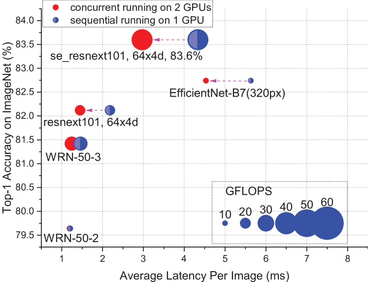
Figure 5: The difference of inference latency between sequential and concurrent running. Test on Tesla V100(s) with mixed precision and batch size 100.

runtime and correlation of small networks after dividing

Runtime and cosine similarity of outputs of different networks are shown in Table VIII. Corresponding accuracy and FLOPs of these networks can be found in Table II. For big networks, concurrent running (small networks run in parallel) can get obvious speedup at runtime compared to sequential running. For small networks, additional data loading, data pre-processing (still runs in sequence) and data transferring (CPU$\Leftrightarrow$GPU, GPU$\Leftrightarrow$GPU) will occupy most of the time. The runtime is also related to the intrinsic structure of networks (e.g., depthwise convolution) and the runtime implementation of the code framework. The speedup of concurrent running with different networks on ImageNet is shown in Figure 5.

In Table VIII, we also show the average cosine similarity of outputs of different small networks. There is no obvious relationship between the similarity of outputs and the gain for different networks. For example, (ResNeXt-19, $S=4$) has similarity $0.89$ and gain $1.55\%$ in accuracy, while (EfficientNet-B0, $S=4$) has similarity $0.79$ and gain $0.65\%$ in accuracy. (EfficientNet-B3, $S=4$) with similarity $0.85$ also has a larger gain $1.48\%$ than (EfficientNet-B0, $S=4$). Lower similarity scores do not always mean more gains in accuracy.

Ensemble of ensemble models

The ensemble of divided networks can also achieve better accuracy-efficiency trade-offs (better performance with roughly the same parameters) than the original single model. The testing results are shown in Figure 6. For Top-1 accuracy, the ensemble of ensemble models obtains better performance than single models when the number of networks is relatively small. Then the former also reaches the saturation point (plateau) faster than the latter. As for top-5 accuracy, the ensemble of ensemble models always achieves higher accuracy than single models. This shows the robustness of the ensemble of ensemble models. Like other dimensions of model scaling, i.e., width, depth, and resolution, increasing the number of networks will also saturate. Otherwise, we will get a perfect model by increasing the number of networks; it is not practical.

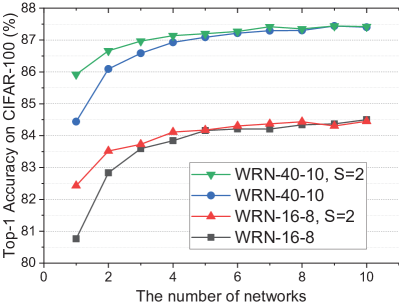
(a) Top-1 Accuracy

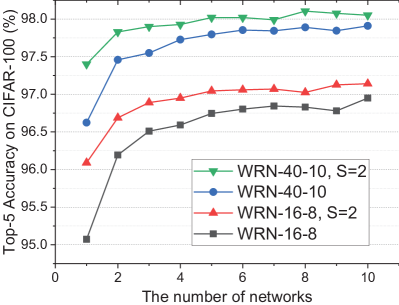
(b) Top-5 Accuracy

Figure 6: Ensemble of ensemble models. {WRN, $S=2$} is treated as a single model. The left is top-1 accuracy, the right is top-5 accuracy.

V Dividing for object detection

We discuss the dividing and co-training strategies for image classification models in the above context. From the experiments on image classification, we can see that dividing and ensemble contributes most to help the system achieve better performance with similar computation costs. In this section, we will explore how dividing and ensemble work on another fundamental computer vision task — object detection.

The overall architecture of our detection system is shown in Figure 7. Without loss of generality, we choose SSD [65] as the object detector and replace its original backbone (feature extractor) — VGG16 [20] with models in Table. IV. We then divide the backbone into $S$ small networks, typically, $S=2$. For simplicity and compatibility with the bounding box regression process of SSD, the detection predictors — extra feature layers and classifiers in SSD share the same weights. After Non-Maximum Suppression (NMS), we obtain the predicted bounding boxes and their associated confidence scores. Furthermore, these predictions from different small detection models are composed to get the final predicted bounding boxes and corresponding confidence scores. To fully utilize the information provided by different detection models, the ensemble method we adopt here is weighted boxes fusion (WBF) [66]. Unlike NMS-based methods [67, 68] which will simply abandon part of the predictions, WBF utilizes all predicted boxes of a certain object from different models to construct a more accurate average box based on the confidence scores of boxes. Such dividing and ensemble methods can be easily extended to other object detectors like YOLO [69].

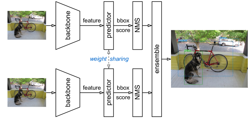
Figure 7: The overall architecture of the detection system with dividing. The two different backbones are obtained from dividing a large network.

TABLE IX: Results of SSD300 on COCO val2017 with dividing and ensemble. Average Precision (AP) and Average Recall (AR) are reported.

			AP, IoU:			AP, Area:			AR, #Dets:			AR, Area:
Backbone	MParams	GFLOPs	0.5:0.95	0.5	0.75	S	M	L	1	10	100	S	M	L
ResNet-50 [70]	23.0	42.3	25.0	42.3	25.7	7.6	26.9	39.9	23.7	34.2	35.8	11.8	39.4	54.8
WRN-50-2	39.3	48.1	30.3	49.7	31.7	10.9	34.1	45.5	27.0	39.5	41.2	16.2	46.9	58.9
WRN-50-2, $S=2$	31.7	45.3	29.9	49.3	31.2	10.5	33.3	45.7	27.0	39.9	42.1	17.1	47.6	60.9
WRN-50-3	64.1	86.8	30.7	51.2	32.0	11.1	34.8	45.9	27.2	39.6	41.4	16.5	46.5	59.9
WRN-50-3, $S=2$	64.3	96.3	31.6	51.5	33.0	11.9	35.6	47.3	28.0	41.2	43.3	18.5	49.2	61.5
ResNeXt-101, 64$\times$4d	68.9	90.1	32.6	53.0	34.1	11.9	36.6	49.6	28.2	41.0	42.8	17.8	48.4	62.4
ResNeXt-101, 64$\times$4d, $S=2$	69.8	100.5	34.1	54.7	35.8	13.5	38.5	52.2	29.3	43.0	45.2	20.4	51.0	65.5

Experiments on object detection are done with SSD300 on MS COCO [71] dataset. The input image is resized to 300$\times$300. Following training schedule of the open-source implementation of NVIDIA [70], we train SSD300 with different backbones on COCO train2017 set for 65 epochs. The COCO train2017 set contains 118K RGB images. The initial learning rate is $0.0026$ and is decayed by 10 at epoch 43 and 54. The optimization algorithm is SGD with a momentum of 0.9. The value of weight decay is 5e-4. After training, the model is validated on COCO val2017 set, which contains 5K images. The backbones are all pre-trained on ImageNet as shown in Table. IV. No test-time augmentations are used.

The results of SSD300 with dividing and ensemble are shown in Table. IX. The dividing strategy also works for SSD on the object detection task. When the backbone is large, dividing and ensemble can bring significant improvements of AP and AR. Especially for the recall of objects with large areas, dividing and ensemble achieve more than +3% AR for (ResNeXt-101, 64$\times$4d, $S=2$) compared to its counterpart. Due to multiple runs of predictors as Figure 7 shows, the FLOPs of the whole system will generally increase after dividing. The numbers of parameters are roughly similar.

VI Conclusion and future work

In this paper, we discuss the accuracy-efficiency trade-offs of increasing the number of networks and demonstrate it is better than purely increasing the depth or width of networks. Along this process, a simple yet effective method — dividing and co-training is proposed to enhance the performance of a single large model. This work potentially introduces some interesting topics in neural network engineering, e.g., designing a flexible framework for asynchronous training of multiple models, more complex deep ensemble and co-training methods, multiple models with different modalities, introducing the idea to NAS (given a specific constrain of FLOPs, how can we design one or several models to get the best performance).

Shuai Zhao received the Master degree in Computer Science from Zhejiang University, Hangzhou, China in 2020, and the Bachelor Degree in Automation from Huazhong University of Science & Technology, Wuhan, China in 2017. His research interests include computer vision and machine learning.

Liguang Zhou received the B.Eng. degree in Electrical Engineering and Automation from China Jiliang University, Hangzhou, China, in 2016, and he is pursuing the Ph.D. degree in Computer Information Engineering at The Chinese of Hong Kong, Shenzhen, China. His research interests include robotic vision, scene understanding, and computational photography.

Wenxiao Wang is an assistant professor, School of Software Technology at Zhejiang University, China. He received the Ph.D. degree in computer science and technology from Zhejiang University in 2022. His research interests include deep learning and computer vision.

Deng Cai is currently a full professor in the College of Computer Science at Zhejiang University, China. He received the Ph.D. degree from University of Illinois at Urbana Champaign. His research interests include machine learning, computer vision, data mining and information retrieval.

Tin Lun LAM (Senior Member, IEEE) received the B.Eng. (First Class Hons.) and Ph.D. degrees in robotics and automation from the Chinese University of Hong Kong, Hong Kong, in 2006 and 2010, respectively. He is currently an Assistant Professor with the Chinese University of Hong Kong, Shenzhen, China, the Executive Deputy Director of the National-Local Joint Engineering Laboratory of Robotics and Intelligent Manufacturing, and the Director of Center for the Intelligent Robots, Shenzhen Institute of Artificial Intelligence and Robotics for Society. He has authored or coauthored two monographs and more than 50 research papers in top-tier international journals and conference proceedings in robotics and AI [IEEE TRANSACTIONS ON ROBOTICS, Journal of Field Robotics, IEEE/ASME TRANSACTIONS ON MECHATRONICS (T-MECH), IEEE ROBOTICS AND AUTOMATION LETTERS, IEEE International Conference on Robotics and Automation, and IEEE/RSJ International Conference on Intelligent Robots and Systems (IROS)]. He holds more than 70 patents. His research interests include multirobot systems, field robotics, and collaborative robotics. Dr. Lam received an IEEE/ASME T-MECH Best Paper Award in 2011 and the IEEE/RSJ IROS Best Paper Award on Robot Mechanisms and Design in 2020.

Yangsheng Xu (Fellow, IEEE) received the B.S.E. and M.S.E. degrees from Zhejiang University, Hangzhou, China, in 1982 and 1984, respectively, and the Ph.D. degree in 1989 from University of Pennsylvania, Philadelphia, PA, USA, all in robotics. He is currently President and Professor of the Chinese University of Hong Kong, Shenzhen, China. His research interests include robotics, intelligent systems, and electric vehicles.

References

- [1] M. Tan and Q. V. Le, “Efficientnet: Rethinking model scaling for convolutional neural networks,” in ICML, 2019.
- [2] S. Zagoruyko and N. Komodakis, “Wide residual networks,” in BMVC, 2016.
- [3] S. Xie, R. B. Girshick, P. Dollár, Z. Tu, and K. He, “Aggregated residual transformations for deep neural networks,” in CVPR, 2017.
- [4] G. Huang, Y. Li, G. Pleiss, Z. Liu, J. E. Hopcroft, and K. Q. Weinberger, “Snapshot ensembles: Train 1, get M for free,” in ICLR, 2017.
- [5] H. Li, X. Wang, and S. Ding, “Research and development of neural network ensembles: a survey,” Artif. Intell. Rev., 2018.
- [6] Y. Liu and X. Yao, “Simultaneous training of negatively correlated neural networks in an ensemble,” IEEE Trans. Syst. Man Cybern. Part B, 1999.
- [7] B. E. Rosen, “Ensemble learning using decorrelated neural networks,” Connection science, 1996.
- [8] S. Tao, “Deep neural network ensembles,” CoRR, 2019.
- [9] D. Kondratyuk, M. Tan, M. Brown, and B. Gong, “When Ensembling Smaller Models is More Efficient than Single Large Models,” arXiv:2005.00570, May 2020.
- [10] Y. Ge, D. Chen, and H. Li, “Mutual mean-teaching: Pseudo label refinery for unsupervised domain adaptation on person re-identification,” in ICLR, 2020.
- [11] T. Yang, S. Zhu, C. Chen, S. Yan, M. Zhang, and A. Willis, “Mutualnet: Adaptive convnet via mutual learning from network width and resolution,” in ECCV, 2020.
- [12] Y. Zhang, T. Xiang, T. M. Hospedales, and H. Lu, “Deep mutual learning,” in CVPR, 2018.
- [13] S. Qiao, W. Shen, Z. Zhang, B. Wang, and A. L. Yuille, “Deep co-training for semi-supervised image recognition,” in ECCV, 2018.
- [14] G. E. Hinton, O. Vinyals, and J. Dean, “Distilling the knowledge in a neural network,” CoRR, vol. abs/1503.02531, 2015.
- [15] O. Russakovsky, J. Deng, H. Su, J. Krause, S. Satheesh, S. Ma, Z. Huang, A. Karpathy, A. Khosla, M. S. Bernstein, A. C. Berg, and F. Li, “Imagenet large scale visual recognition challenge,” IJCV, 2015.
- [16] A. Krizhevsky and G. Hinton, “Learning multiple layers of features from tiny images,” University of Toronto, Toronto, Ontario, Tech. Rep. 0, 2009.
- [17] P. Micikevicius, S. Narang, J. Alben, G. F. Diamos, E. Elsen, D. García, B. Ginsburg, M. Houston, O. Kuchaiev, G. Venkatesh, and H. Wu, “Mixed precision training,” in ICLR, 2018.
- [18] A. Krizhevsky, I. Sutskever, and G. E. Hinton, “Imagenet classification with deep convolutional neural networks,” in NeurIPS, 2012.
- [19] M. Lin, Q. Chen, and S. Yan, “Network in network,” arXiv preprint arXiv:1312.4400, 2013.
- [20] K. Simonyan and A. Zisserman, “Very deep convolutional networks for large-scale image recognition,” in ICLR. arXiv.org, 2015. [Online]. Available: http://arxiv.org/abs/1409.1556
- [21] C. Szegedy, W. Liu, Y. Jia, P. Sermanet, S. E. Reed, D. Anguelov, D. Erhan, V. Vanhoucke, and A. Rabinovich, “Going deeper with convolutions,” in CVPR, 2015.
- [22] K. He, X. Zhang, S. Ren, and J. Sun, “Deep residual learning for image recognition,” in CVPR, 2016.
- [23] F. Chollet, “Xception: Deep learning with depthwise separable convolutions,” in CVPR, 2017.
- [24] B. Zoph and Q. V. Le, “Neural architecture search with reinforcement learning,” in ICLR, 2017.
- [25] C. Liu, B. Zoph, M. Neumann, J. Shlens, W. Hua, L. Li, L. Fei-Fei, A. L. Yuille, J. Huang, and K. Murphy, “Progressive neural architecture search,” in ECCV, 2018.
- [26] H. Liu, K. Simonyan, and Y. Yang, “DARTS: differentiable architecture search,” in ICLR, 2019.
- [27] H. Zhang, C. Wu, Z. Zhang, Y. Zhu, Z. Zhang, H. Lin, Y. Sun, T. He, J. Muller, R. Manmatha, M. Li, and A. Smola, “Resnest: Split-attention networks,” arXiv preprint arXiv:2004.08955, 2020.
- [28] N. Srivastava, G. E. Hinton, A. Krizhevsky, I. Sutskever, and R. Salakhutdinov, “Dropout: a simple way to prevent neural networks from overfitting,” J. Mach. Learn. Res., vol. 15, no. 1, pp. 1929–1958, 2014.
- [29] J. Yu, L. Yang, N. Xu, J. Yang, and T. S. Huang, “Slimmable neural networks,” in ICLR. OpenReview.net, 2019, pp. 1–12. [Online]. Available: https://openreview.net/forum?id=H1gMCsAqY7
- [30] J. Yu and T. S. Huang, “Universally slimmable networks and improved training techniques,” in ICCV, 2019.
- [31] B. L. Smith and J. T. MacGregor, Collaborative Learning: A Sourcebook for Higher Education. Office of Educational Research and Improvement (ED), Washington, DC: ERIC, 1992, ch. What is collaborative learning.
- [32] G. Song and W. Chai, “Collaborative learning for deep neural networks,” in NeurIPS, 2018.
- [33] A. Blum and T. M. Mitchell, “Combining labeled and unlabeled data with co-training,” in COLT. ACM, 1998.
- [34] T. Batra and D. Parikh, “Cooperative learning with visual attributes,” CoRR, vol. abs/1705.05512, 2017.
- [35] A. Paszke, S. Gross, F. Massa, A. Lerer, J. Bradbury, G. Chanan, T. Killeen, Z. Lin, N. Gimelshein, L. Antiga, A. Desmaison, A. Kopf, E. Yang, Z. DeVito, M. Raison, A. Tejani, S. Chilamkurthy, B. Steiner, L. Fang, J. Bai, and S. Chintala, “Pytorch: An imperative style, high-performance deep learning library,” in NeurIPS, 2019.
- [36] M. Sandler, A. G. Howard, M. Zhu, A. Zhmoginov, and L. Chen, “Mobilenetv2: Inverted residuals and linear bottlenecks,” in CVPR, 2018.
- [37] J. Hu, L. Shen, and G. Sun, “Squeeze-and-excitation networks,” in CVPR, 2018.
- [38] G. Huang, Z. Liu, L. van der Maaten, and K. Q. Weinberger, “Densely connected convolutional networks,” in CVPR, 2017.
- [39] D. Han, J. Kim, and J. Kim, “Deep pyramidal residual networks,” in CVPR, 2017.
- [40] Y. Yamada, M. Iwamura, T. Akiba, and K. Kise, “Shakedrop regularization for deep residual learning,” IEEE Access, 2019.
- [41] G. Huang, Y. Sun, Z. Liu, D. Sedra, and K. Q. Weinberger, “Deep networks with stochastic depth,” in ECCV, 2016.
- [42] A. Krogh and J. A. Hertz, “A simple weight decay can improve generalization,” in NeurIPS, 1991.
- [43] G. Zhang, C. Wang, B. Xu, and R. B. Grosse, “Three mechanisms of weight decay regularization,” in ICLR, 2019.
- [44] A. Golatkar, A. Achille, and S. Soatto, “Time matters in regularizing deep networks: Weight decay and data augmentation affect early learning dynamics, matter little near convergence,” in NeurIPS, 2019.
- [45] NVIDIA, “Cuda toolkit documentation v11.1.0,” https://docs.nvidia.com/cuda/cuda-c-programming-guide/index.html#streams, 2020.
- [46] N. Ueda and R. Nakano, “Generalization error of ensemble estimators,” in Proceedings of International Conference on Neural Networks, 1996.
- [47] Z. Zhong, L. Zheng, G. Kang, S. Li, and Y. Yang, “Random erasing data augmentation,” in AAAI, 2020.
- [48] E. D. Cubuk, B. Zoph, D. Mane, V. Vasudevan, and Q. V. Le, “Autoaugment: Learning augmentation strategies from data,” in CVPR, 2019.
- [49] S. Laine and T. Aila, “Temporal ensembling for semi-supervised learning,” in ICLR, 2017.
- [50] P. Goyal, P. Dollár, R. B. Girshick, P. Noordhuis, L. Wesolowski, A. Kyrola, A. Tulloch, Y. Jia, and K. He, “Accurate, large minibatch SGD: training imagenet in 1 hour,” CoRR, vol. abs/1706.02677, 2017.
- [51] T. He, Z. Zhang, H. Zhang, Z. Zhang, J. Xie, and M. Li, “Bag of tricks for image classification with convolutional neural networks,” CoRR, vol. abs/1812.01187, 2018.
- [52] T. Devries and G. W. Taylor, “Improved regularization of convolutional neural networks with cutout,” CoRR, vol. abs/1708.04552, 2017.
- [53] K. He, X. Zhang, S. Ren, and J. Sun, “Identity mappings in deep residual networks,” in ECCV, 2016.
- [54] H. Zhang, M. Cissé, Y. N. Dauphin, and D. Lopez-Paz, “mixup: Beyond empirical risk minimization,” in ICLR, 2018.
- [55] C. Szegedy, V. Vanhoucke, S. Ioffe, J. Shlens, and Z. Wojna, “Rethinking the inception architecture for computer vision,” in CVPR. IEEE Computer Society, 2016.
- [56] S. Ioffe and C. Szegedy, “Batch normalization: Accelerating deep network training by reducing internal covariate shift,” in ICML, 2015.
- [57] K. He, X. Zhang, S. Ren, and J. Sun, “Delving deep into rectifiers: Surpassing human-level performance on imagenet classification,” in ICCV, 2015.
- [58] Y. Nesterov, “A method for unconstrained convex minimization problem with the rate of convergence o (1/k^ 2),” in Doklady an ussr, vol. 269, 1 1983, pp. 543–547.
- [59] E. D. Cubuk, B. Zoph, J. Shlens, and Q. V. Le, “Randaugment: Practical automated data augmentation with a reduced search space,” arXiv preprint arXiv:1909.13719, 2019.
- [60] H. Zhang, Y. N. Dauphin, and T. Ma, “Fixup initialization: Residual learning without normalization,” in ICLR, 2019.
- [61] S. Lim, I. Kim, T. Kim, C. Kim, and S. Kim, “Fast autoaugment,” in NeurIPS, 2019.
- [62] X. Gastaldi, “Shake-shake regularization,” CoRR, vol. abs/1705.07485, 2017.
- [63] M. Berman, H. Jégou, V. Andrea, I. Kokkinos, and M. Douze, “MultiGrain: a unified image embedding for classes and instances,” arXiv e-prints, 2019.
- [64] E. Real, A. Aggarwal, Y. Huang, and Q. V. Le, “Regularized evolution for image classifier architecture search,” in AAAI, 2019.
- [65] W. Liu, D. Anguelov, D. Erhan, C. Szegedy, S. E. Reed, C. Fu, and A. C. Berg, “SSD: single shot multibox detector,” in ECCV, 2016.
- [66] R. Solovyev, W. Wang, and T. Gabruseva, “Weighted boxes fusion: Ensembling boxes from different object detection models,” Image and Vision Computing, 2021.
- [67] Á. Casado-García and J. Heras, “Ensemble methods for object detection,” in ECAI, 2020.
- [68] N. Bodla, B. Singh, R. Chellappa, and L. S. Davis, “Soft-nms - improving object detection with one line of code,” in ICCV, 2017.
- [69] J. Redmon, S. K. Divvala, R. B. Girshick, and A. Farhadi, “You only look once: Unified, real-time object detection,” in CVPR, 2016.
- [70] NVIDIA, “Deep learning examples for tensor cores,” 2020, https://github.com/NVIDIA/DeepLearningExamples/tree/master/PyTorch/Detection/SSD.
- [71] T. Lin, M. Maire, S. J. Belongie, J. Hays, P. Perona, D. Ramanan, P. Dollár, and C. L. Zitnick, “Microsoft COCO: common objects in context,” in ECCV, 2014.