Feature Space Singularity for Out-of-Distribution Detection

Abstract

Out-of-Distribution (OoD) detection is important for building safe artificial intelligence systems. However, current OoD detection methods still cannot meet the performance requirements for practical deployment. In this paper, we propose a simple yet effective algorithm based on a novel observation: in a trained neural network, OoD samples with bounded norms well concentrate in the feature space. We call the center of OoD features the Feature Space Singularity (FSS), and denote the distance of a sample feature to FSS as FSSD. Then, OoD samples can be identified by taking a threshold on the FSSD. Our analysis of the phenomenon reveals why our algorithm works. We demonstrate that our algorithm achieves state-of-the-art performance on various OoD detection benchmarks. Besides, FSSD also enjoys robustness to slight corruption in test data and can be further enhanced by ensembling. These make FSSD a promising algorithm to be employed in real world. We release our code at https://github.com/megvii-research/FSSD_OoD_Detection.

Introduction

Empirical risk minimization fits a statistical model on a training set which is independently sampled from the data distribution. As a result, the yielded model is expected to generalize to in-distribution data drawn from the same distribution. However, in real applications, it is inevitable for a model to make predictions on Out-of-Distribution (OoD) data instead of in-distribution data on which the model is trained. This can lead to fatal errors such as over-confident or ridiculous predictions  (Hein, Andriushchenko, and Bitterwolf 2018; Rabanser, Günnemann, and Lipton 2019). Therefore, it is crucial to understand the uncertainty of models and automatically detect OoD data. In applications like autonomous driving and medical services, if the model knows what it does not know, human intervention can be sought and security can be significantly improved.

Consider one particular example of OoD detection: some high-quality human face images are given as in-distribution data (training set for OoD detector), and we are interested in filtering out non-faces and low quality faces from a large pool of data in the wild (test set) in order to ensure reliable prediction. One natural solution is to remove test samples far from the training data in some designated distances (Lee et al. 2018b; van Amersfoort et al. 2020). However, calculating the distance to the whole training set needs a formidable amount of computation without some special design in feature and architecture, e.g., training a RBF network (van Amersfoort et al. 2020).

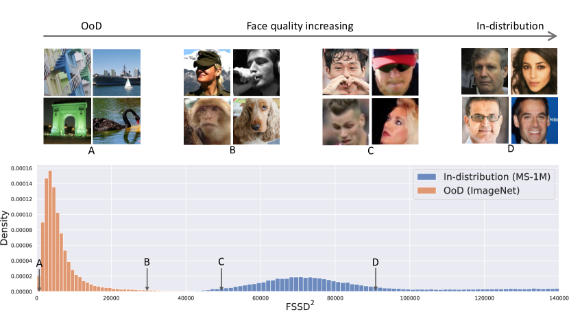
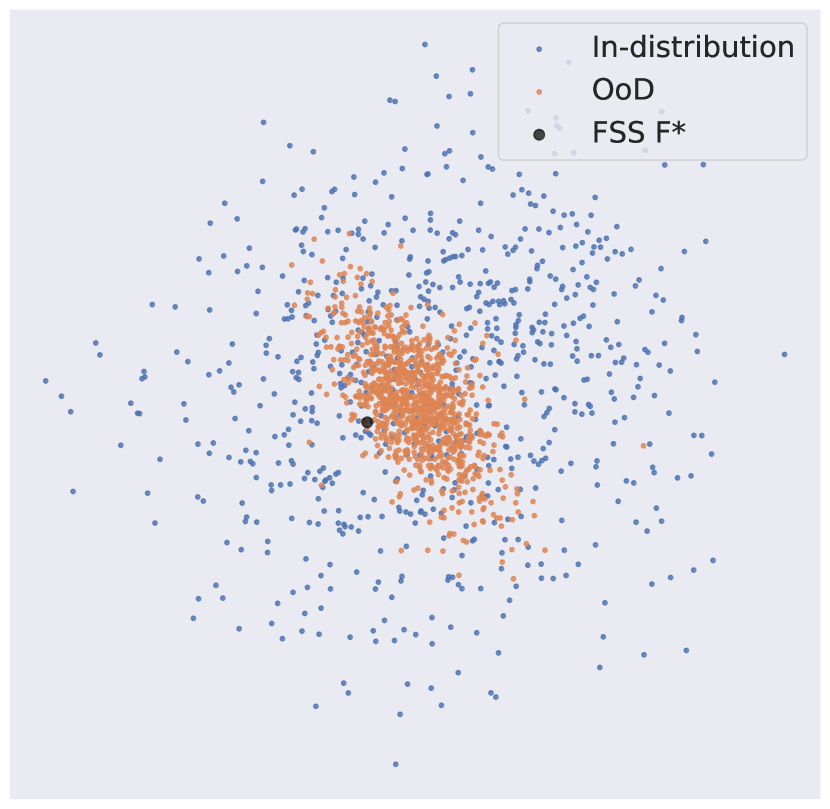
Figure 1: Left: Histogram of FSS Distance (FSSD) of MS1M (in-distribution) and ImageNet (OoD). Exemplar images are shown at different FSSDs. We can see that FSSD reflects the OoD degree: as the FSSD increases, images change from non-faces and pseudo-faces, to low-quality faces and high-quality faces. Right: Principle components of features from the penultimate layer. The spatial relationship among FSS, OoD data, and in-distribution data is shown.

In this paper, we present a simple yet effective distance-based solution, which neither computes the distance to the training data nor performs extra model training than a standard classifier.

Our approach is based on a novel observation about OoD samples:

In a trained neural network, OoD samples with bounded norms well concentrate in the feature space of the neural network.

In Figure 1, we show an example where OoD features from ImageNet (Russakovsky et al. 2015) concentrate in a neural network trained on the facial dataset MS-1M (Guo et al. 2016). Figure 2 and 3 provide more examples of this phenomenon. In fact, we find this phenomenon to be universal in most training configurations for most datasets.

To be more precise, for a given feature extractor $F_{\theta}$ trained on in-distribution data, the observation states that there exists a point $F^{\ast}$ in the output space of $F_{\theta}$ such that $\left\|F_{\theta}\left(x\right)-F^{\ast}\right\|$ is small for $x\in\mathcal{X}_{\text{OoD}}$, where $\mathcal{X}_{\text{OoD}}$ is the set of OoD samples. We call $F^{\ast}$ the Feature Space Singularity (FSS). Moreover, we discover the FSS Distance (FSSD)

$$\text{FSSD}\left(x\right):=\left\|F_{\theta}\left(x\right)-F^{\ast}\right\|$$ (1)

can reflect the degree of OoD, and thus can be readily used as a metric for OoD detection.

Our analysis demonstrates that this phenomenon can be explained by the training dynamics. The key observation is that FSSD can be seen as an approximate movement of $F_{\theta_{t}}\left(x\right)$ during training, where $F^{*}$ is the initial concentration point of the features. The difference in the moving speed $\frac{\mathop{\mathrm{d}\!}F_{\theta_{t}}\left(x\right)}{\mathop{\mathrm{d}\!}t}$ stems from the different similarity to the training data measured by the inner product of the gradients. Moreover, this similarity measure varies according to the architecture of the feature extractor.

We demonstrate the effectiveness of our proposed method with multiple neural networks (LeNet (LeCun and Cortes 2010), ResNet (He et al. 2016), ResNeXt (Xie et al. 2017), LSTM (Hochreiter and Schmidhuber 1997)) trained on various datasets for classification (FashionMNIST (Xiao, Rasul, and Vollgraf 2017), CIFAR10 (Krizhevsky 2009), ImageNet (Russakovsky et al. 2015), CelebA (Liu et al. 2015), MS-1M (Guo et al. 2016), bacteria genome dataset (Ren et al. 2019)) with varying training set sizes. We show that FSSD achieves state-of-the-art performance on almost all the considered benchmarks. Moreover, the performance margin between FSSD and other methods increases as the size of the training set increases. In particular, on large-scale benchmarks (CelebA and MS-1M), FSSD advances the AUROC by about 5%. We also evaluate the robustness of our algorithm when test images are corrupted. We find that our algorithm can still reliably detect OoD samples under this circumstance. Finally, we investigate the effects of ensembling FSSDs from different layers of a single neural network and multiple trained netowrks.

We summarize our contributions as follows.

• We observe that in feature spaces of trained networks OoD samples concentrate near a point (FSS), and the distance from a sample feature to FSS (FSSD) measures the degree of OoD (Section 1).

• We analyze the concentration phenomenon by analyzing the dynamics of in-distribution and OoD features during training (Section 2).

• We introduce the FSSD algorithm (Section 3) which achieves state-of-the-art performance on various OoD detection benchmarks with considerable robustness (Section 4).

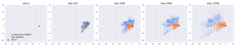
(a) The dynamics of features $F_{\theta_{t}}\left(x\right)$.

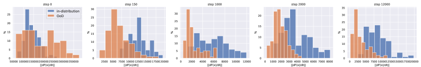
(b) The norm of the derivative, i.e., "moving speed", of last-layer feature vector at different time steps.

Figure 2: We show first two principle components of the feature vector and the L2 norm of the derivatives (Equation (3)). Features and derivatives are calculated from the last fully-connected layer of a LeNet trained on MNIST (in-distribution). We feed in FashionMNIST data as OoD samples. At initialization, features of both in-distribution and OoD samples concentrate near FSS $F^{\ast}$. After training, features of in-distribution samples are pulled away from FSS $F^{\ast}$, while features of OoD samples remain close to FSS $F^{\ast}$. Similar dynamics of the softmax layer on in-distribution data was observed by (Li, Zhao, and Scheidegger 2020).

Analyzing and Understanding the Concentration Phenomenon

In this section, we analyze the concentration phenomenon. The key observation is that during training, the features of the training data are supervised to move away from the initial point, and the moving speeds of features of other data depend on their similarity to the training data. Specifically, this similarity is measured by the inner product of the gradients. Therefore, data that are dissimilar to the training data will move little and concentrate in the feature space. This is how FSSD identifies OoD data.

To see this, we derive the training dynamics of the feature vectors. We denote $F_{\theta}:\mathbb{R}^{a}\rightarrow\mathbb{R}^{b}$ as the feature extractor which maps inputs to features and $G_{\phi}:\mathbb{R}^{b}\rightarrow\mathbb{R}^{c}$ to be the map from features to outputs. The two mappings are parameterized by $\theta$ and $\phi$ respectively. The corresponding loss function can be denoted as $\mathcal{L}_{\phi}\left(F_{\theta}\left(x_{1}\right),\cdots,F_{\theta}\left(x_{M}\right)\right)$. A popular choice is $\mathcal{L}_{\phi}\left(F_{\theta}\left(x_{1}\right),\cdots,F_{\theta}\left(x_{M}\right)\right)=\sum_{m=1}^{M}\ell\left(G_{\phi}\left(F_{\theta}\left(x_{m}\right)\right),y_{m}\right)/M$, where $\ell$ is the cross entropy loss or the mean squared error. Then, the gradient descent dynamics of $\theta$ is

$$\frac{\mathop{\mathrm{d}\!}\theta_{t}}{\mathop{\mathrm{d}\!}t}= -\frac{\mathop{\partial\!}\mathcal{L}_{\phi}}{\mathop{\partial\!}\theta_{t}}\left(F_{\theta_{t}}\left(x_{1}\right),\cdots,F_{\theta_{t}}\left(x_{M}\right)\right)$$ (2)

$$= -\sum_{m=1}^{M}\frac{\mathop{\partial\!}F_{\theta_{t}}\left(x_{m}\right)^{\mathsf{T}}}{\mathop{\partial\!}\theta_{t}}\mathop{\partial_{m}\!}\mathcal{L}_{\phi},$$

where $\mathop{\partial_{m}\!}\mathcal{L}_{\phi}=\frac{\mathop{\partial\!}\mathcal{L}_{\phi}}{\mathop{\partial\!}F_{\theta_{t}}\left(x_{m}\right)}\in\mathbb{R}^{b}$ is the backward propagation gradient and subscript $t$ is the training time. The dynamics of the feature extractor $F_{\theta}$ as a function is therefore

$$\frac{\mathop{\mathrm{d}\!}F_{\theta_{t}}\left(x\right)}{\mathop{\mathrm{d}\!}t}= \frac{\mathop{\partial\!}F_{\theta_{t}}\left(x\right)}{\mathop{\partial\!}\theta_{t}}\frac{\mathop{\mathrm{d}\!}\theta_{t}}{\mathop{\mathrm{d}\!}t}$$ (3)

$$= -\sum_{m=1}^{M}\frac{\mathop{\partial\!}F_{\theta_{t}}\left(x\right)}{\mathop{\partial\!}\theta_{t}}\frac{\mathop{\partial\!}F_{\theta_{t}}\left(x_{m}\right)^{\mathsf{T}}}{\mathop{\partial\!}\theta_{t}}\mathop{\partial_{m}\!}\mathcal{L}_{\phi}.$$

From Equation (3), we can see that the relative moving speed of the feature $F_{\theta_{t}}\left(x\right)$ depends on the inner product of the gradient on parameters between $x$ and the training data $x_{m}$. Note here $\mathop{\partial_{m}\!}\mathcal{L}_{\phi}$ is the same for all $x$. Since FSSD defined in Equation 1 can be seen as the integration of $\frac{\mathop{\mathrm{d}\!}F_{\theta_{t}}\left(x\right)}{\mathop{\mathrm{d}\!}t}$ when the initial value $F_{\theta_{0}}\left(x\right)$ is $F^{*}$ for all x, FSSD(x) will also be small when the derivative, i.e., the moving speed, is small.

In Figure 2, we show both the features and their moving speeds of in-distribution and OoD data at different steps during training. We can see that although in-distribution and OoD data are indistinguishable at step 0, they are quickly separated since the moving speeds of in-distribution data are larger than those of OoD data (Figure 2(b)) and thus the accumulated movements of in-distribution data are also larger than those of OoD data (Figure 2(a)). In Figure 3, we show examples of the initial concentration of features in LeNet and ResNet-34 for MNIST vs. FashionMNIST and CIFAR10 vs. SVHN dataset pairs respectively. Empirically, we find the concentration of both in-distribution and OoD features at the initial stage to be the common case for most popular architectures using random initialization. We show more examples on our Github page.

As we’ve mentioned, Equation (3) demonstrates that the difference in the moving speed of $F_{\theta_{t}}\left(x\right)$ stems from difference in $\Theta_{t}\left(x,x_{m}\right):=\frac{\mathop{\partial\!}F_{\theta_{t}}\left(x\right)}{\mathop{\partial\!}\theta_{t}}\frac{\mathop{\partial\!}F_{\theta_{t}}\left(x_{m}\right)^{\mathsf{T}}}{\mathop{\partial\!}\theta_{t}}$. We want to further point out that $\Theta_{t}\left(x,x_{m}\right)$ is effectively acting as a kernel that measures the similarity between $x$ and $x_{m}$. In fact, when the network width is infinite, $\Theta_{t}\left(x,x_{m}\right)$ will converge to a time-independent term $\Theta(x,x_{m})$, which is called neural tangent kernel (NTK) (Jacot, Gabriel, and Hongler 2018; Li and Liang 2018; Cao and Gu 2020). In this way, FSSD can be seen as a kernel regression result:

$$\text{FSSD}\left(x\right) \mathrel{\leavevmode\hbox to48.45pt{\vbox to29.67pt{\text{[drawing]}}}}\big{\|}F_{\theta_{t}}\left(x\right)-F_{\theta_{0}}\left(x\right)\big{\|} F^{\ast}\!\approx\!F_{\theta_{0}}\left(x\right) F^{\ast}\!\approx\!F_{\theta_{0}}\left(x\right)$$ (4)

$$=\left\|\sum_{m=1}^{M}\int_{0}^{T}\Theta_{t}\left(x,x_{m}\right)\mathop{\partial_{m}\!}\mathcal{L}_{\phi}\mathop{\mathrm{d}\!}t\right\|$$

$$\approx\left\|\sum_{m=1}^{M}\Theta\left(x,x_{m}\right)\nu_{m}\right\|,$$

where $\nu_{m}=\int_{0}^{T}\mathop{\partial_{m}\!}\mathcal{L}_{\phi}\mathop{\mathrm{d}\!}t$.

This indicates that the similarity described by the inner product $\Theta_{t}\left(x,x_{m}\right):=\frac{\mathop{\partial\!}F_{\theta_{t}}\left(x\right)}{\mathop{\partial\!}\theta_{t}}\frac{\mathop{\partial\!}F_{\theta_{t}}\left(x_{m}\right)^{\mathsf{T}}}{\mathop{\partial\!}\theta_{t}}$ might enjoy similar properties to commonly used kernels such as RBF kernel, which diminishes as the distance between $x$ and $x_{m}$ increases. Moreover, since the neural tangent kernel depends on the neural architecture, this kernel interpretation also suggests that feature extractors of different architectures, including different layers, can have different properties and measure different aspects of the similarity between $x$ and $x_{m}$. We can see this more clearly later in the investigation of FSSD in different layers.

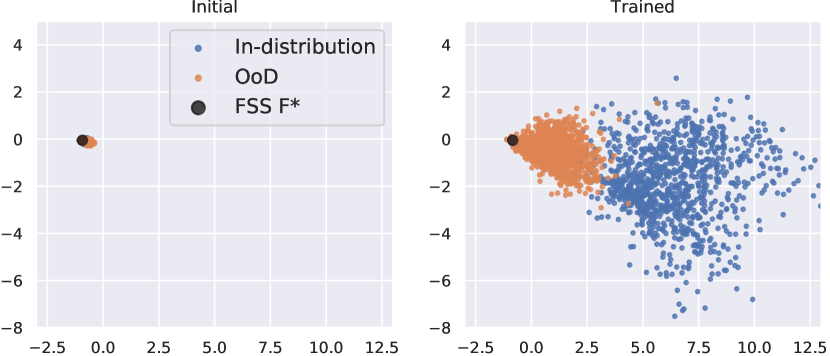
(a) MNIST vs. FMNIST

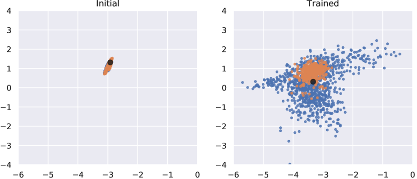
(b) CIFAR10 vs. SVHN

Figure 3: Both in-distribution and OoD samples are clustered in the feature space of $F_{\theta_{0}}\left(x\right)$ at initialization. Moreover, $F^{\ast}\approx F_{\theta_{0}}\left(x\right)$ for $x\in\mathcal{X}_{\text{OoD}}\cup\mathcal{X}_{\text{in-dist}}$.

Our Algorithm

Based on this phenomenon, we can now construct our OoD detection algorithm. Since the uniform noise input can be considered to possess the highest degree of OoD, we use the center of their features as the FSS $F^{\ast}$. The FSSD can then be calculated using Equation (1). Note this calculation of FSS $F^{\ast}$ is independent from the choice of in-distribution and OoD datasets. When such natural choice of uniform noise is unavailable, we can choose FSS $F^{\ast}$ to be the center of features of OoD validation data instead.

Since a single forward-pass computation through the network can give us features from each layer, it is also convenient to calculate FSSDs from different layers and ensemble them as $\text{FSSD-Ensem}\left(x\right)=\sum_{k=1}^{K}\alpha_{k}\text{FSSD}^{\left(k\right)}\left(x\right)$. The ensemble weights $\alpha_{k}$ can be determined using logistic regression on some validation data as in (Lee et al. 2018b) (see Evaluation section in Experiments). In later experiments, if not specified, we use the ensembled FSSD from all layers. We note that it is also possible to ensemble FSSDs from different architectures or multiple training snapshots (Xie, Xu, and Zhang 2013; Huang et al. 2017). This may further enhance the performance of OoD detection. We investigate the effect of ensembling in the next section.

Beside, we also adopt input pre-processing as in  (Liang, Li, and Srikant 2018; Lee et al. 2018b) . The idea is to add small perturbations to the test samples in order to increase the in-distribution score. It is shown in (Liang, Li, and Srikant 2018; Kamoi and Kobayashi 2020) that in-distribution data are more sensitive to such perturbation and it can therefore enlarge the score gap between in-distribution and OoD samples. In particular, we perturb as $\tilde{x}=x+\epsilon\mathop{\text{sign}}\left(\nabla_{x}\text{FSSD}\left(x\right)\right)$ and take $\text{FSSD}\left(\tilde{x}\right)$ as the final score.

We present the pseudo-code of computing $\text{FSSD-Ensem}\left(x\right)$ in Algorithm 1.

Input: Test samples $\bm{x}=\left\{x^{\text{test}}_{n}\right\}{}_{n=1}^{N}$, noise samples $\left\{x^{\text{noise}}_{s}\right\}{}_{s=1}^{S}$, ensemble weights $\alpha_{k}$, perturbation magnitude $\epsilon$,

Input:  feature extractors $\big{\{}F_{\left(k\right)}\big{\}}{}_{k=1}^{K}$

for each feature extractor $\big{\{}F_{\left(k\right)}\big{\}}{}_{k=1}^{K}$ do

       1. Estimate FSS $F^{\ast}_{\left(k\right)}=\sum_{s=1}^{S}F_{\left(k\right)}\big{(}x^{\text{noise}}_{s}\big{)}/S$, where $x^{\text{noise}}_{s}\sim\mathcal{U}[0,1]$, $s=1,\cdots,S$

       2. Add perturbation to test sample: $\tilde{\bm{{x}}}=\bm{x}+\epsilon\mathop{\text{sign}}(\nabla_{\bm{x}}\big{\|}F_{\left(k\right)}\left(\bm{x}\right)-F^{\ast}_{\left(k\right)}\big{\|})$

       3. Calculate $\text{FSSD}^{(k)}\left(\bm{x}\right)=\big{\|}F_{\left(k\right)}\left(\tilde{\bm{x}}\right)-F^{\ast}_{\left(k\right)}\big{\|}$

      

end for

Return $\text{FSSD-Ensem}\left(\bm{x}\right)=\sum_{k=1}^{K}\alpha_{k}\ \text{FSSD}^{(k)}\left(\bm{x}\right)$

Algorithm 1 Computation of FSSD-Ensem

Experiments

In this section, we investigate the performance of our FSSD algorithm on various OoD detection benchmarks.

Table 1: OoD detection benchmarks used in our experiments.

	In-distribution						OoD		Data type
	Dataset	#Classes		#Samples			Dataset	#Samples
		(Train/	Test)	(Train/	Test)			(Test)
A	FMNIST	10/	10	60k/	10k		MNIST	10k	Image
B	CIFAR10	10/	10	50k/	10k		SVHN	26k	Image
C	ImageNet (dogs)	50/	50	50k/	10k		ImageNet (non-dogs)	10k	Image
D	ImageNet	1000/	1000	1281.2k/	50k		ImageNet-C	50k	Image
E	CelebA (not blurry)	10122/	10122	153.8k/	38.5k		CelebA (blurry)	10.3k	Image
F	MS-1M	64736/	16184	2923.6k/	50k		IJB-C	50k	Image
G	Genome (before 2011)	10/	10	1000k/	1000k		Genome (after 2016)	6000k	Sequence

Setup

Benchmarks

To conduct a thorough test of our method, we consider a wide variety of OoD detection benchmarks. In particular, we consider different scales of datasets and different types of data. We consider different scales of datasets because large scale datasets tend to have more classes which can introduce more ambiguous data. The ambiguous data are of high classification uncertainty, but are not out-of-distribution. We list the benchmarks in Table 1.

We first consider two common benchmarks from previous OoD detection literature (van Amersfoort et al. 2020; Ren et al. 2019): (A) FMNIST (Xiao, Rasul, and Vollgraf 2017) vs. MNIST (LeCun and Cortes 2010) and (B) CIFAR10 (Krizhevsky 2009) vs. SVHN (Netzer et al. 2011). They are known to be challenging for many methods (Ren et al. 2019; Nalisnick et al. 2019a). (C) We also construct ImageNet (dogs), a subset of ImageNet  (Russakovsky et al. 2015) , as in-distribution data. The OoD data are non-dog images from ImageNet.

For large-scale problems, we consider three benchmarks. (D) We train models on ImageNet and detect corrupted images from the ImageNet-C dataset (Hendrycks and Dietterich 2019). We test each method on 80 sets of corruptions (16 types and 5 levels). (E) We train models on face images without the “blurry” attribute from CelebA (Liu et al. 2015) and detect face images with the “blurry” attribute. (F) We train models on web images of celebrities from MS-Celeb-1M (MS-1M) (Guo et al. 2016) and detect video captures from IJB-C (Maze et al. 2018) which in general have lower quality due to pose, illumination, and resolution issues. We also consider (G) the bacteria genome benchmark introduced by (Ren et al. 2019), which consists of sequence data.

To train models on in-distribution datasets, we follow previous works (Lee et al. 2018b) to train LeNet on FMNIST and ResNet with 34 layers on CIFAR10, ImageNet, and ImageNet (dogs). For two face recognition datasets (CelebA and MS-1M), we train ResNeXt with 50 layers. For the genome sequence dataset, we use an character embedding layer and two Bidirectional LSTM layers (Schuster and Paliwal 1997).

Compared methods

We compare our method with the following six common methods for OoD detection. Base: the baseline method using the maximum softmax probability $p\left(\hat{y}\middle|x\right)$ (Hendrycks and Gimpel 2017). ODIN: temperature scaling on logits and input pre-processing (Liang, Li, and Srikant 2018). Maha: Mahalanobis distance of the sample feature to the closest class-conditional Gaussian distribution which is estimated from the training data (Lee et al. 2018b). In our experiments, we follow  (Lee et al. 2018b) to use both feature (layer) ensemble and input pre-processing. DE: Deep Ensemble which averages the softmax probability predictions from multiple independently trained classifiers  (Lakshminarayanan, Pritzel, and Blundell 2017). In our experiments, we take the average of 5 classifiers by default. MCD: Monte-Carlo Dropout that uses dropout during both training and inference (Gal and Ghahramani 2016). We follow  (Ovadia et al. 2019) to dropout convolutional layers. For OoD detection, we calculate both the mean and the variance of 32 independent predictions and choose the better one to report. OE: Outlier exposure that explicitly enforces uniform probability prediction on an auxiliary dataset of outliers  (Hendrycks, Mazeika, and Dietterich 2019). For the choice of auxiliary datsets, we use KMNIST (Clanuwat et al. 2018) for benchmark A, CelebA (Liu et al. 2015) for benchmark C, and ImageNet-1K (Russakovsky et al. 2015) for benchmark B, E, F. We do not evaluate OE on the sequence benchmark, since we can not find a reasonable auxiliary dataset. We remark here that Base, ODIN, and FSSD can be deployed directly with a trained neural network, MCD needs a trained neural network with dropout layers, while DE needs multiple trained classifiers. Besides, Maha needs to use the training data during OoD detection on test data and OE trains a neural network either from scratch or by fine-tuning to utilize the auxiliary dataset.

Evaluation

We follow (Ren et al. 2019; Hendrycks, Mazeika, and Dietterich 2019) to use the following metrics to assess the performance of OoD detection. AUROC: Area Under the Receiver Operating Characteristic curve. AUPRC: Area Under the Precision-Recall Curve. FPR80: False Positive Rate when the true positive rate is 80%.

For hyper-parameter tuning, we follow  (Lee et al. 2018b; Ren et al. 2019; Liang, Li, and Srikant 2018) to use a separate validation set, which consists of 1,000 images from each in-distribution and OoD data pair. Ensemble weights $\alpha_{k}$ for FSSD from different layers are extracted from a logistic regression model, which is trained using nested cross validation within the validation set as in (Lee et al. 2018b; Ma et al. 2018). The same procedure is performed on Maha for fair comparison. The perturbation magnitude $\epsilon$ of input pre-processing for ODIN, Maha, and FSSD is searched from 0 to 0.2 with step size 0.01. The temperature $T$ of ODIN is chosen from 1, 10, 100, and 1000, and the dropout rate of MCD is chosen from 0.01, 0.02, 0.05, 0.1, 0.2, 0.3, 0.4, and 0.5.

Main results

The main results are presented in Table 2 and Figure 4. In Table 2, we can see that larger datasets entail greater difficulty in OoD detection. Notably, the advantage of FSSD over other methods increases as the dataset size increases. Other methods like Maha and OE perform well on some small benchmarks, but have large variance across different datasets. In comparison, FSSD maintains great performance on these benchmarks. On the genome sequence dataset, we also observe that FSSD outperforms other methods. These results show that FSSD is a promising effective method for a wide range of applications.

Inspired by (Ovadia et al. 2019), we also evaluate the methods on the ability of detecting distributional dataset shift like Gaussian noise and JPEG artifacts. Figure 4 shows the means and quartiles of AUROC of the compared methods over 16 types of corruptions on 5 corruption levels. We can observe that for each method, the performance of OoD detection increases as the level of corruption increases, while FSSD enjoys the highest AUROC and much less variation over different types of corruptions. The CelebA benchmark also evaluates the methods on detecting the dataset shift of the attribute “blurry”. However, all methods including FSSD do not perform very well. There are two possible reasons: (1) the attribute “blurry” of CelebA may be annotated not clearly enough; (2) the blurs in the wild may be more difficult to detect than the simulated blurs in ImageNet-C. Overall, we can see that FSSD can more reliably detect different kinds of distributional shifts.

Table 2: Main results. All values are in %.

	Datasets (Architecture)	Metrics	Base	ODIN	Maha	DE	MCD	OE	FSSD
Small-scale benchmarks	FMNIST vs. MNIST (LeNet)	AUROC	77.3	96.9	99.6	83.9	81.7	99.6	99.6
		AUPRC	79.2	93.0	99.7	83.3	85.3	99.6	99.7
		FPR80	43.5	2.5	0.0	27.5	36.8	0.0	0.0
	CIFAR10 vs. SVHN (ResNet34)	AUROC	89.9	96.7	99.1	93.7	96.7	90.4	99.5
		AUPRC	85.4	92.5	98.1	90.6	93.9	89.8	99.5
		FPR80	10.1	4.7	0.3	3.7	2.4	12.5	0.4
	ImageNet dogs vs. non-dogs (ResNet34)	AUROC	88.5	90.8	83.3	89.0	67.2	92.5	93.1
		AUPRC	86.1	88.6	83.0	89.0	66.9	92.6	92.5
		FPR80	19.5	15.2	30.1	18.8	59.2	7.9	10.2
Large-scale benchmarks	CelebA non-blurry vs. blurry (ResNeXt50)	AUROC	71.7	73.3	73.9	74.5	69.8	71.5	78.3
		AUPRC	89.9	91.4	90.9	91.4	88.7	90.7	92.8
		FPR80	52.0	50.3	46.0	47.1	53.2	54.2	39.2
	MS-1M vs. IJB-C (ResNeXt50)	AUROC	60.0	61.3	82.5	63.0	65.5	52.6	86.7
		AUPRC	53.3	55.9	80.6	56.1	59.4	46.6	86.1
		FPR80	61.8	59.4	29.6	56.7	58.8	64.2	22.1
Sequence benchmark	Bacteria Genome (LSTM)	AUROC	69.6	70.6	70.4	70.0	69.3	NA	74.8
		AUPRC	69.9	71.9	69.3	56.0	70.2	NA	75.8
		FPR80	57.4	55.9	53.7	30.0	58.3	NA	47.4

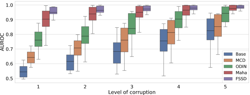
Figure 4: Comparison of AUROC on ImageNet vs. ImageNet-C. FSSD enjoys the highest mean and the least variance across all corruption levels.

Robustness

In practice, it is possible that the test data are slightly corrupted or shifted due to the change of data source, e.g., from lab to real world. We evaluate the ability to distinguish in-distribution data from OoD data when test data (both in-distribution and OoD) are slightly corrupted. Note that we still use non-corrupted data during network training and hyper-parameter tuning. We apply Gaussian noise and impulse noise, two typical corruptions, with varying levels. Test results on CIFAR10 vs. SVHN and ImageNet dogs vs. non-dogs are shown in Figure 5. We can see that FSSD is robust to corruptions presented in test images, while other methods may degrade.

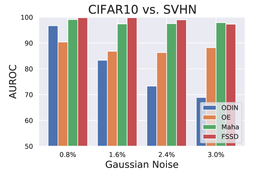
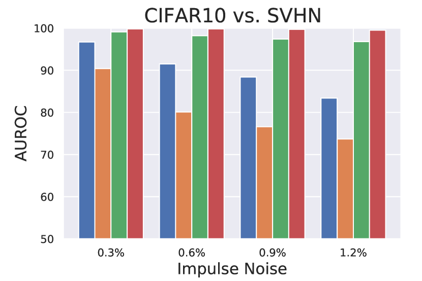
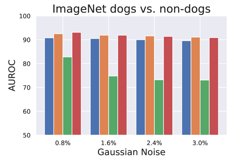
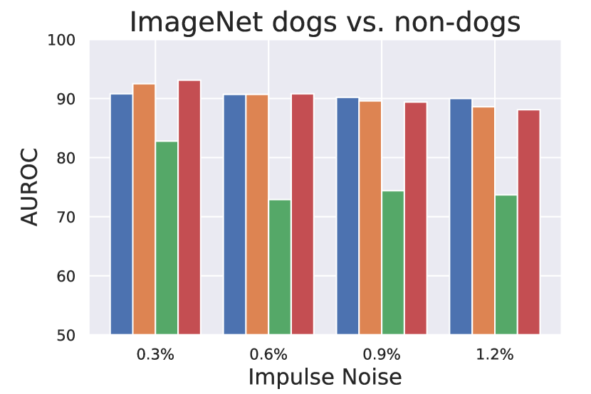
Figure 5: Comparison of OoD detection robustness among methods on slightly corrupted test data.

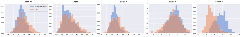
(a) ImageNet (dogs) vs. ImageNet (non-dogs)

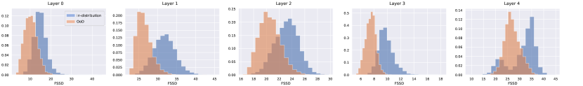
(b) CIFAR10 vs. SVHN

Figure 6: FSSDs from different layers behave differently. Each row contains FSSD histograms extracted from different layers of a trained neural network. FSSDs of ImageNet (dogs) and ImageNet (non-dogs) are similar in early layers; while FSSDs of CIFAR10 and SVHN differ in all the layers. This can be explained by the fact that ImageNet (dogs) and ImageNet (non-dogs) are similar in low-level statistics since they are sampled from the same dataset, and that FSSDs in early layers capture more of the difference in low-level statistics.

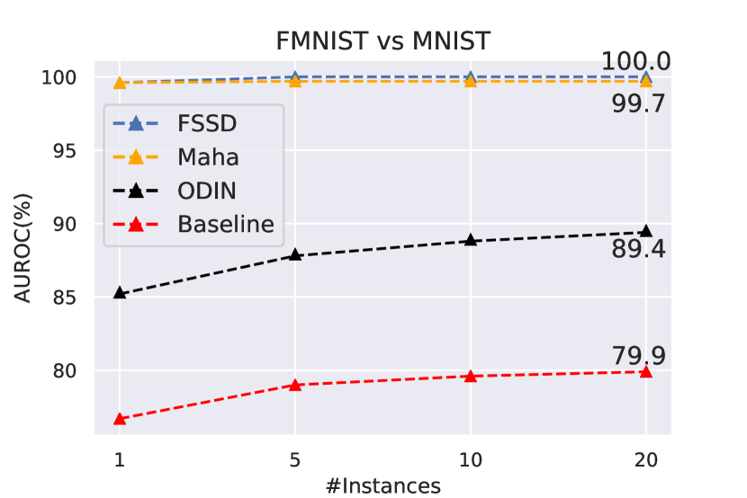
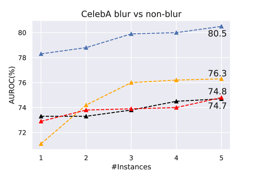
Figure 7: Comparison of network ensembles of Base, ODIN, Maha, and FSSD scores.

Effects of ensemble

During our experiments, we find that the ensemble plays an important role in enhancing the performance of FSSD. Previous studies show that an important issue for ensemble-based algorithms is enforcing diversity (Lakshminarayanan, Pritzel, and Blundell 2017). In our case, we find that FSSD has high diversity across different layers, and benefit from such diversity to reach higher performance. In Figure 6, we find that FSSD in different layers are working differently. This can be explained by previous works on understanding neural networks by visualizing the different representations learned by low and deep layers of a neural network (Zeiler and Fergus 2014; Zhou et al. 2015). Generally, FSSDs from deep layers reflect more high-level features and FSSDs from early layers reflect more low-level statistics. ImageNet (dogs) and ImageNet (non-dogs) are from the same dataset (ImageNet), and are therefore similar in terms of low-level statistics; while the differences between CIFAR10 and SVHN are in all different levels. From the perspective of kernel interpretation, this means that the neural tangent kernels of different layers diversify well and allow the ensemble of FSSD to capture different aspects of the discrepancy between the test data and training data. We show more examples of FSSDs in different layers on our Github page.

Furthermore, Figure 7 demonstrates that the performance of FSSD can be further boosted by using network ensembles. Considering the low computational cost of ensembling FSSD, this shows FSSD can be a promising method in scenarios that require high-performance OoD detectors.

Related works

Out-of-distribution detection

According to different understandings of OoD samples, previous OoD detection methods can be summarized into four categories.

(1) Some methods regard OoD samples as those with uniform probability prediction across classes (Hein, Andriushchenko, and Bitterwolf 2018; Hendrycks and Gimpel 2017; Liang, Li, and Srikant 2018; Lee et al. 2018a; Hein and Andriushchenko 2017; Meinke and Hein 2020) and treat the test samples with high entropy or low maximum prediction probability as OoD data. Since these methods are based on prediction, they run the risk of mis-classifying ambiguous data as OoD samples, e.g., when there are thousands of classes in a large-scale dataset.

(2) OoD samples can also be characterized as samples with high epistemic uncertainty which reflects the lack of information on these samples (Lakshminarayanan, Pritzel, and Blundell 2017; Gal and Ghahramani 2016; Blundell et al. 2015). Specifically, we can propagate the uncertainty of models to the uncertainty of predictions, which characterizes the level of OoD. MCD and DE are two popular choices of this type. However, it is reported that current epistemic uncertainty estimations may noticeably degrade under dataset distributional shift (Ovadia et al. 2019). Our experiments on detecting ImageNet-C from ImageNet (Figure 4) confirm this.

(3) When the density of data can be approximated, e.g., using generative models (Kingma and Dhariwal 2018; Salimans et al. 2017), OoD samples can be classified as those with low density. Recent works provide many inspiring insights on how to improve this idea (Ren et al. 2019; Nalisnick et al. 2019b; Serrà et al. 2020). However, these methods typically have extra training difficulty incurred by large generative models.

(4) There are also works designing non-Euclidean metrics to compare test samples to training samples, and regard those with higher distances to training samples as OoD samples (Lee et al. 2018b; van Amersfoort et al. 2020; Kamoi and Kobayashi 2020; Lakshminarayanan et al. 2020). Our approach resembles this type most. Instead of comparing test samples to training samples, we compare the features of the test samples to the center of OoD features.

Non-Lipschitz property of neural networks

Many previous works have reported that the trained neural networks are not Lipschitz continuous (Behrmann et al. 2019; van Amersfoort et al. 2020; Lakshminarayanan et al. 2020). Some OoD detection methods claim that adding Lipschitz constraint may help improve OoD detection performance (van Amersfoort et al. 2020; Lakshminarayanan et al. 2020).  (Bietti and Mairal 2019) also demonstrated that the NTK kernel mappings of ReLU networks are non-Lipschitz.

Instead of adding Lipschitz constraint, this work utilizes the non-Lipschitz property of neural networks for OoD detection. In fact, the feature space singularity provides us with new understandings of the non-Lipschitz region in the input space, i.e., inputs that are dissimilar to the training data in terms of the NTK. In the future, it is interesting to further investigate the non-Lipschitz properties of neural networks, e.g., non-Lipschitz behaviours in different layers and how the inductive bias of NTK influences the OoD detection using FSSD.

Conclusion

In this work, we propose a new OoD detection algorithm based on a novel observation that OoD samples concentrate in the feature space of a trained neural network. We provide analysis and understanding of the concentration phenomenon by analyzing the training dynamics both theoretically and empirically and further interpreted the algorithm with the neural tangent kernel. We demonstrate that our algorithm is state-of-the-art in detection performance and is robust to measurement noise. Our further investigation on the effect of ensemble reveals diversity in layer ensembles and shows promising performance of network ensembles. In summary, we hope that our work can provide new insights for understanding properties of neural networks and add an alternative simple and effective OoD detection method to the safe AI deployment toolkits.

References

- Behrmann et al. (2019) Behrmann, J.; Grathwohl, W.; Chen, R. T. Q.; Duvenaud, D.; and Jacobsen, J.-H. 2019. Invertible Residual Networks. In International Conference on Machine Learning, 573–582. PMLR. URL http://proceedings.mlr.press/v97/behrmann19a.html. ISSN: 2640-3498.
- Bietti and Mairal (2019) Bietti, A.; and Mairal, J. 2019. On the Inductive Bias of Neural Tangent Kernels. arXiv:1905.12173 [cs, stat] URL http://arxiv.org/abs/1905.12173. ArXiv: 1905.12173.
- Blundell et al. (2015) Blundell, C.; Cornebise, J.; Kavukcuoglu, K.; and Wierstra, D. 2015. Weight Uncertainty in Neural Network. volume 37 of Proceedings of Machine Learning Research, 1613–1622. Lille, France: PMLR. URL http://proceedings.mlr.press/v37/blundell15.html.
- Cao and Gu (2020) Cao, Y.; and Gu, Q. 2020. Generalization Error Bounds of Gradient Descent for Learning Over-Parameterized Deep ReLU Networks. In The Thirty-Fourth AAAI Conference on Artificial Intelligence, 3349–3356. AAAI Press. URL https://aaai.org/ojs/index.php/AAAI/article/view/5736.
- Clanuwat et al. (2018) Clanuwat, T.; Bober-Irizar, M.; Kitamoto, A.; Lamb, A.; Yamamoto, K.; and Ha, D. 2018. Deep Learning for Classical Japanese Literature.
- Gal and Ghahramani (2016) Gal, Y.; and Ghahramani, Z. 2016. Dropout as a Bayesian Approximation: Representing Model Uncertainty in Deep Learning. volume 48 of Proceedings of Machine Learning Research, 1050–1059. New York, New York, USA: PMLR. URL http://proceedings.mlr.press/v48/gal16.html.
- Guo et al. (2016) Guo, Y.; Zhang, L.; Hu, Y.; He, X.; and Gao, J. 2016. MS-Celeb-1M: A Dataset and Benchmark for Large-Scale Face Recognition. In Leibe, B.; Matas, J.; Sebe, N.; and Welling, M., eds., Computer Vision – ECCV 2016, volume 9907, 87–102. Cham: Springer International Publishing. ISBN 978-3-319-46486-2 978-3-319-46487-9. doi:10.1007/978-3-319-46487-9_6. URL http://link.springer.com/10.1007/978-3-319-46487-9_6. Series Title: Lecture Notes in Computer Science.
- He et al. (2016) He, K.; Zhang, X.; Ren, S.; and Sun, J. 2016. Deep Residual Learning for Image Recognition. In 2016 IEEE Conference on Computer Vision and Pattern Recognition (CVPR), 770–778. Las Vegas, NV, USA: IEEE. ISBN 978-1-4673-8851-1. doi:10.1109/CVPR.2016.90. URL http://ieeexplore.ieee.org/document/7780459/.
- Hein and Andriushchenko (2017) Hein, M.; and Andriushchenko, M. 2017. Formal Guarantees on the Robustness of a Classifier against Adversarial Manipulation. In Guyon, I.; Luxburg, U. V.; Bengio, S.; Wallach, H.; Fergus, R.; Vishwanathan, S.; and Garnett, R., eds., Advances in Neural Information Processing Systems 30, 2266–2276. Curran Associates, Inc. URL http://papers.nips.cc/paper/6821-formal-guarantees-on-the-robustness-of-a-classifier-against-adversarial-manipulation.pdf.
- Hein, Andriushchenko, and Bitterwolf (2018) Hein, M.; Andriushchenko, M.; and Bitterwolf, J. 2018. Why ReLU Networks Yield High-Confidence Predictions Far Away From the Training Data and How to Mitigate the Problem. 2019 IEEE/CVF Conference on Computer Vision and Pattern Recognition (CVPR) 41–50.
- Hendrycks and Dietterich (2019) Hendrycks, D.; and Dietterich, T. 2019. Benchmarking Neural Network Robustness to Common Corruptions and Perturbations. Proceedings of the International Conference on Learning Representations .
- Hendrycks and Gimpel (2017) Hendrycks, D.; and Gimpel, K. 2017. A Baseline for Detecting Misclassified and Out-of-Distribution Examples in Neural Networks. Proceedings of International Conference on Learning Representations .
- Hendrycks, Mazeika, and Dietterich (2019) Hendrycks, D.; Mazeika, M.; and Dietterich, T. 2019. Deep Anomaly Detection with Outlier Exposure. In International Conference on Learning Representations. URL https://openreview.net/forum?id=HyxCxhRcY7.
- Hochreiter and Schmidhuber (1997) Hochreiter, S.; and Schmidhuber, J. 1997. Long Short-Term Memory. Neural Comput. 9(8): 1735–1780. ISSN 0899-7667. doi:10.1162/neco.1997.9.8.1735. URL https://doi.org/10.1162/neco.1997.9.8.1735.
- Huang et al. (2017) Huang, G.; Li, Y.; Pleiss, G.; Liu, Z.; Hopcroft, J. E.; and Weinberger, K. Q. 2017. Snapshot Ensembles: Train 1, get M for free. CoRR abs/1704.00109. URL http://arxiv.org/abs/1704.00109.
- Jacot, Gabriel, and Hongler (2018) Jacot, A.; Gabriel, F.; and Hongler, C. 2018. Neural Tangent Kernel: Convergence and Generalization in Neural Networks. In Bengio, S.; Wallach, H.; Larochelle, H.; Grauman, K.; Cesa-Bianchi, N.; and Garnett, R., eds., Advances in Neural Information Processing Systems 31, 8571–8580. Curran Associates, Inc. URL http://papers.nips.cc/paper/8076-neural-tangent-kernel-convergence-and-generalization-in-neural-networks.pdf.
- Kamoi and Kobayashi (2020) Kamoi, R.; and Kobayashi, K. 2020. Why is the Mahalanobis Distance Effective for Anomaly Detection? arXiv:2003.00402 [cs, stat] URL http://arxiv.org/abs/2003.00402. ArXiv: 2003.00402.
- Kingma and Dhariwal (2018) Kingma, D. P.; and Dhariwal, P. 2018. Glow: Generative Flow with Invertible 1x1 Convolutions. In Bengio, S.; Wallach, H.; Larochelle, H.; Grauman, K.; Cesa-Bianchi, N.; and Garnett, R., eds., Advances in Neural Information Processing Systems 31, 10215–10224. Curran Associates, Inc. URL http://papers.nips.cc/paper/8224-glow-generative-flow-with-invertible-1x1-convolutions.pdf.
- Krizhevsky (2009) Krizhevsky, A. 2009. Learning multiple layers of features from tiny images. Technical report.
- Lakshminarayanan, Pritzel, and Blundell (2017) Lakshminarayanan, B.; Pritzel, A.; and Blundell, C. 2017. Simple and Scalable Predictive Uncertainty Estimation using Deep Ensembles. In Guyon, I.; Luxburg, U. V.; Bengio, S.; Wallach, H.; Fergus, R.; Vishwanathan, S.; and Garnett, R., eds., Advances in Neural Information Processing Systems 30, 6402–6413. Curran Associates, Inc. URL http://papers.nips.cc/paper/7219-simple-and-scalable-predictive-uncertainty-estimation-using-deep-ensembles.pdf.
- Lakshminarayanan et al. (2020) Lakshminarayanan, B.; Tran, D.; Liu, J.; Padhy, S.; Bedrax-Weiss, T.; and Lin, Z. 2020. Simple and Principled Uncertainty Estimation with Deterministic Deep Learning via Distance Awareness. In Advances in Neural Information Processing Systems 33.
- LeCun and Cortes (2010) LeCun, Y.; and Cortes, C. 2010. MNIST handwritten digit database URL http://yann.lecun.com/exdb/mnist/.
- Lee et al. (2018a) Lee, K.; Lee, H.; Lee, K.; and Shin, J. 2018a. Training Confidence-calibrated Classifiers for Detecting Out-of-Distribution Samples. In International Conference on Learning Representations. URL https://openreview.net/forum?id=ryiAv2xAZ.
- Lee et al. (2018b) Lee, K.; Lee, K.; Lee, H.; and Shin, J. 2018b. A Simple Unified Framework for Detecting Out-of-Distribution Samples and Adversarial Attacks. In Proceedings of the 32nd International Conference on Neural Information Processing Systems, NIPS’18, 7167–7177. Red Hook, NY, USA: Curran Associates Inc.
- Li, Zhao, and Scheidegger (2020) Li, M.; Zhao, Z.; and Scheidegger, C. 2020. Visualizing Neural Networks with the Grand Tour. Distill doi:10.23915/distill.00025. Https://distill.pub/2020/grand-tour.
- Li and Liang (2018) Li, Y.; and Liang, Y. 2018. Learning Overparameterized Neural Networks via Stochastic Gradient Descent on Structured Data. In Proceedings of the 32nd International Conference on Neural Information Processing Systems, NIPS’18, 8168–8177. Red Hook, NY, USA: Curran Associates Inc.
- Liang, Li, and Srikant (2018) Liang, S.; Li, Y.; and Srikant, R. 2018. Enhancing The Reliability of Out-of-distribution Image Detection in Neural Networks. In International Conference on Learning Representations. URL https://openreview.net/forum?id=H1VGkIxRZ.
- Liu et al. (2015) Liu, Z.; Luo, P.; Wang, X.; and Tang, X. 2015. Deep Learning Face Attributes in the Wild. In Proceedings of International Conference on Computer Vision (ICCV).
- Ma et al. (2018) Ma, X.; Li, B.; Wang, Y.; Erfani, S. M.; Wijewickrema, S.; Schoenebeck, G.; Houle, M. E.; Song, D.; and Bailey, J. 2018. Characterizing Adversarial Subspaces Using Local Intrinsic Dimensionality. In International Conference on Learning Representations. URL https://openreview.net/forum?id=B1gJ1L2aW.
- Maze et al. (2018) Maze, B.; Adams, J.; Duncan, J. A.; Kalka, N.; Miller, T.; Otto, C.; Jain, A. K.; Niggel, W. T.; Anderson, J.; Cheney, J.; and Grother, P. 2018. IARPA Janus Benchmark - C: Face Dataset and Protocol. In 2018 International Conference on Biometrics (ICB), 158–165. Gold Coast, QLD: IEEE. ISBN 978-1-5386-4285-6. doi:10.1109/ICB2018.2018.00033. URL https://ieeexplore.ieee.org/document/8411217/.
- Meinke and Hein (2020) Meinke, A.; and Hein, M. 2020. Towards neural networks that provably know when they don’t know. In International Conference on Learning Representations. URL https://openreview.net/forum?id=ByxGkySKwH.
- Nalisnick et al. (2019a) Nalisnick, E.; Matsukawa, A.; Teh, Y. W.; Gorur, D.; and Lakshminarayanan, B. 2019a. Do Deep Generative Models Know What They Don’t Know? In International Conference on Learning Representations. URL https://openreview.net/forum?id=H1xwNhCcYm.
- Nalisnick et al. (2019b) Nalisnick, E.; Matsukawa, A.; Teh, Y. W.; and Lakshminarayanan, B. 2019b. Detecting Out-of-Distribution Inputs to Deep Generative Models Using Typicality.
- Netzer et al. (2011) Netzer, Y.; Wang, T.; Coates, A.; Bissacco, A.; Wu, B.; and Ng, A. Y. 2011. Reading Digits in Natural Images with Unsupervised Feature Learning. In NIPS Workshop on Deep Learning and Unsupervised Feature Learning 2011. URL http://ufldl.stanford.edu/housenumbers/nips2011_housenumbers.pdf.
- Ovadia et al. (2019) Ovadia, Y.; Fertig, E.; Ren, J.; Nado, Z.; Sculley, D.; Nowozin, S.; Dillon, J. V.; Lakshminarayanan, B.; and Snoek, J. 2019. Can You Trust Your Model’s Uncertainty? Evaluating Predictive Uncertainty Under Dataset Shift. In NeurIPS.
- Rabanser, Günnemann, and Lipton (2019) Rabanser, S.; Günnemann, S.; and Lipton, Z. 2019. Failing Loudly: An Empirical Study of Methods for Detecting Dataset Shift. In Wallach, H.; Larochelle, H.; Beygelzimer, A.; Alché-Buc, F. d.; Fox, E.; and Garnett, R., eds., Advances in Neural Information Processing Systems 32, 1396–1408. Curran Associates, Inc. URL http://papers.nips.cc/paper/8420-failing-loudly-an-empirical-study-of-methods-for-detecting-dataset-shift.pdf.
- Ren et al. (2019) Ren, J.; Liu, P. J.; Fertig, E.; Snoek, J.; Poplin, R.; Depristo, M.; Dillon, J.; and Lakshminarayanan, B. 2019. Likelihood Ratios for Out-of-Distribution Detection. In Wallach, H.; Larochelle, H.; Beygelzimer, A.; Alché-Buc, F. d.; Fox, E.; and Garnett, R., eds., Advances in Neural Information Processing Systems 32, 14707–14718. Curran Associates, Inc. URL http://papers.nips.cc/paper/9611-likelihood-ratios-for-out-of-distribution-detection.pdf.
- Russakovsky et al. (2015) Russakovsky, O.; Deng, J.; Su, H.; Krause, J.; Satheesh, S.; Ma, S.; Huang, Z.; Karpathy, A.; Khosla, A.; Bernstein, M.; Berg, A. C.; and Fei-Fei, L. 2015. ImageNet Large Scale Visual Recognition Challenge. International Journal of Computer Vision (IJCV) 115(3): 211–252. doi:10.1007/s11263-015-0816-y.
- Salimans et al. (2017) Salimans, T.; Karpathy, A.; Chen, X.; and Kingma, D. P. 2017. PixelCNN++: A PixelCNN Implementation with Discretized Logistic Mixture Likelihood and Other Modifications. In ICLR.
- Schuster and Paliwal (1997) Schuster, M.; and Paliwal, K. 1997. Bidirectional Recurrent Neural Networks. Trans. Sig. Proc. 45(11): 2673–2681. ISSN 1053-587X. doi:10.1109/78.650093. URL https://doi.org/10.1109/78.650093.
- Serrà et al. (2020) Serrà, J.; Álvarez, D.; Gómez, V.; Slizovskaia, O.; Núñez, J. F.; and Luque, J. 2020. Input Complexity and Out-of-distribution Detection with Likelihood-based Generative Models. In International Conference on Learning Representations. URL https://openreview.net/forum?id=SyxIWpVYvr.
- van Amersfoort et al. (2020) van Amersfoort, J.; Smith, L.; Teh, Y. W.; and Gal, Y. 2020. Simple and Scalable Epistemic Uncertainty Estimation Using a Single Deep Deterministic Neural Network.
- Xiao, Rasul, and Vollgraf (2017) Xiao, H.; Rasul, K.; and Vollgraf, R. 2017. Fashion-MNIST: a Novel Image Dataset for Benchmarking Machine Learning Algorithms.
- Xie, Xu, and Zhang (2013) Xie, J.; Xu, B.; and Zhang, C. 2013. Horizontal and Vertical Ensemble with Deep Representation for Classification. CoRR abs/1306.2759. URL http://arxiv.org/abs/1306.2759.
- Xie et al. (2017) Xie, S.; Girshick, R.; Dollar, P.; Tu, Z.; and He, K. 2017. Aggregated Residual Transformations for Deep Neural Networks. In 2017 IEEE Conference on Computer Vision and Pattern Recognition (CVPR), 5987–5995. Honolulu, HI: IEEE. ISBN 978-1-5386-0457-1. doi:10.1109/CVPR.2017.634. URL http://ieeexplore.ieee.org/document/8100117/.
- Zeiler and Fergus (2014) Zeiler, M.; and Fergus, R. 2014. Visualizing and understanding convolutional networks. In Computer Vision, ECCV 2014 - 13th European Conference, Proceedings, number PART 1 in Lecture Notes in Computer Science (including subseries Lecture Notes in Artificial Intelligence and Lecture Notes in Bioinformatics), 818–833. Springer Verlag. ISBN 9783319105895. doi:10.1007/978-3-319-10590-1_53. 13th European Conference on Computer Vision, ECCV 2014 ; Conference date: 06-09-2014 Through 12-09-2014.
- Zhou et al. (2015) Zhou, B.; Khosla, A.; Lapedriza, A.; Oliva, A.; and Torralba, A. 2015. Object Detectors Emerge in Deep Scene CNNs. In International Conference on Learning Representations (ICLR).