Abstract

We study the critical $O(3)$ model using the numerical conformal bootstrap. In particular, we use a recently developed cutting-surface algorithm to efficiently map out the allowed space of CFT data from correlators involving the leading $O(3)$ singlet $s$, vector $\phi$, and rank-2 symmetric tensor $t$. We determine their scaling dimensions to be $(\Delta_{s},\Delta_{\phi},\Delta_{t})=(0.518942(51),1.59489(59),1.20954(23))$, and also bound various OPE coefficients. We additionally introduce a new “tip-finding” algorithm to compute an upper bound on the leading rank-4 symmetric tensor $t_{4}$, which we find to be relevant with $\Delta_{t_{4}}<2.99056$. The conformal bootstrap thus provides a numerical proof that systems described by the critical $O(3)$ model, such as classical Heisenberg ferromagnets at the Curie transition, are unstable to cubic anisotropy.

1 Introduction

Numerical bootstrap methods [1, 2] (see [3, 4] for recent reviews) have led to powerful new results in the study of conformal field theories (CFTs). In [5, 6] we developed an approach to large-scale bootstrap problems which allowed for precise determinations of the CFT data of the 3d critical ${O}(2)$ model. In this work, we continue the exploration of large-scale bootstrap problems by applying the technology introduced in [5] to the study of the 3d critical $O(3)$ model.

Concretely, we apply these methods to study correlation functions of the lowest-dimension singlet, vector, and rank-2 scalars in the three-dimensional critical $O(3)$ model. Using the “cutting surface” algorithm introduced in [5], we compute the allowed region for the CFT data of these leading scalar operators. Our results, together with comparisons to results from Monte Carlo simulations, are summarized in table 1. We also introduce a new algorithm and software implementation called tiptop, which allows us to efficiently test allowed gaps for other operators across this region. We use it to determine an upper bound on the dimension of the lowest-dimension rank-4 scalar.

The 3d $O(3)$ model is a well-studied renormalization group (RG) fixed point, and its critical exponents have been computed using many methods, both theoretical and experimental. This model describes the critical behavior of isotropic magnets, such as the Curie transition in isotropic ferromagnets, and antiferromagnets at the Néel transition point. Moreover, since disorder corresponds to an irrelevant perturbation, the model also describes isotropic magnets with quenched disorder.

One of the main open questions about the $O(3)$ model is its stability under cubic deformations. The majority of magnets present in nature are indeed not isotropic: this means that the microscopic Hamiltonian describing the system in the ultraviolet (UV) is not invariant under the full $O(3)$ symmetry group but only under a discrete subgroup, such as the cubic symmetry group. This implies that additional terms will be generated at the microscopic level that are invariant under cubic symmetry but transform in a non-trivial representation of $O(3)$. If any of those deformations turn out to be relevant, the $O(3)$ fixed point would be unstable and could not be reached without further tuning in the UV theory. The attractive, stable, fixed point would instead be the 3d cubic model. Field theory computations and Monte Carlo simulations have shown that these two models have very similar critical exponents: hence, if the cubic perturbation is relevant, it should be very close to marginality and the RG flow connecting the two theories is very short. We will come back to this point in section 1.1.1.

CFT data	method	value	ref
$\Delta_{s}$	MC	1.5948(2)	[7]
	CB	1.5957(55)	[8]
	CB	1.59488(81)	this work
$\Delta_{\phi}$	MC	0.518920(25)	[7]
	CB	0.51928(62)	[8]
	CB	0.518936(67)	this work
$\Delta_{t}$	MC	1.2094(3)	[9]
	CB	$1.2095(55^{*})$	[10]
	CB	1.20954(32)	this work
$\Delta_{t_{4}}$	MC	2.987(4)	[9]
	CB	$<2.99056$	this work
$\lambda_{\phi\phi s}$	CB	$0.5244(11^{*})$	[8]
	CB	$0.524261(59^{*})$	this work
$\lambda_{sss}$	CB	$0.499(12^{*})$	[8]
	CB	$0.5055(11^{*})$	this work
$\lambda_{tts}$	CB	$0.98348(39^{*})$	this work
$\lambda_{\phi\phi t}$	CB	$0.87451(22^{*})$	this work
$\lambda_{ttt}$	CB	$1.49957(49^{*})$	this work

Table 1: Comparison of conformal bootstrap (CB) results with previous determinations from Monte Carlo (MC) simulations. We denote the leading rank-0, rank-1, rank-2, and rank-4 scalars by $s,\phi,t,t_{4}$, respectively. Bold uncertainties correspond to rigorous intervals from bootstrap bounds. Uncertainties marked with a ^∗ indicate that the value is estimated non-rigorously by sampling points.

We give a definite answer to the above question: the $O(3)$ model is unstable under cubic deformations. This information is encoded in the dimension of the lowest rank-4 scalar ${t_{4}}$, which in the $O(3)$ model satisfies $\Delta_{t_{4}}<3$. As we will discuss, this implies that the $O(3)$ model is also unstable with respect to the biconal fixed point with $\mathbb{Z}_{2}\times O(2)$ symmetry. Relevance of $t_{4}$ has been previously suggested by Monte Carlo [9] and perturbative expansions [11], but the proximity to marginality and near degeneracy of the critical exponents between the cubic, biconal, and $O(3)$ fixed points makes this a subtle question ideal for the precision and rigor of the conformal bootstrap.

1.1 Theoretical approaches to the 3d $O(3)$ model

We start by briefly reviewing past approaches to the 3d $O(3)$ model, including field theory studies, Monte Carlo, and past results obtained by conformal bootstrap techniques. We also describe related models and motivate the calculations in this work.

The simplest continuum field theory in the $O(3)$ universality class is the theory of a scalar field $\vec{\phi}$ transforming in the fundamental representation of $O(3)$ with Lagrangian

$$\mathcal{L} =\frac{1}{2}|\partial\vec{\phi}|^{2}+\frac{1}{2}m^{2}|\vec{\phi}|^{2}+\frac{g}{4!}|\vec{\phi}|^{4}\,.$$ (1)

A large negative mass-squared for the scalar induces spontaneous symmetry breaking and leads to the ordered phase, while a large positive mass-squared leads to the disordered phase. The critical point is achieved by tuning the UV mass so that the infrared (IR) correlation length diverges. The $\beta$ function of the coupling $g$ has been computed in the $\varepsilon-$expansion and in a fixed-dimension scheme. After a Borel-resummation, both methods predict the existence of an IR stable fixed point. We will review these results in the next sections.

The IR limit of the above field theory captures the same physics as the Heisenberg model. This model consists of a lattice of classical spins $\vec{S}_{i}$, which can take values on a three-dimensional sphere. The Hamiltonian has only nearest-neighbor interactions:

$$\mathcal{H}=-J\sum_{\langle i,j\rangle}\vec{S}_{i}\cdot\vec{S}_{j}+H\sum_{i}S_{i}^{3}\,,$$ (2)

where we also introduced an external magnetic field $H$ in the third ($z$)-direction. When the parameter $J$ is positive, the ground state corresponds to all spins aligned, corresponding to ferromagnets. When $J<0$, the energy is minimized when neighboring spins are anti-aligned, corresponding to antiferromagnets.

For small $J$, the line $H=0$ separates a ferromagnetic phase from the paramagnetic one. This line represents a first-order transition and terminates at a value $J=J_{c}$, where the correlation length of the system diverges, and the transition becomes second order. For $J>J_{c}$, there is only a disordered phase. At $J=J_{c}$, the theory in the IR is in the same universality class of the field theory defined in (1). The critical exponents are related to operator dimensions at the fixed point as

$$\Delta_{\phi}=\frac{1+\eta}{2}\,,\qquad\Delta_{s}=3-\frac{1}{\nu}\,,\qquad\Delta_{t}=3-Y_{2}\,.$$ (3)

Here, $s\sim|\vec{\phi}|^{2}$ denotes the lowest-dimension singlet scalar, while $t_{ij}\sim(\phi_{i}\phi_{j}-\text{trace})$ denotes the lowest rank-2 scalar. More generically the exponents $Y_{r}$ are associated to the dimensions of the lowest rank-$r$ scalar operator. In the ${O}(N)$ model, the dimension of the lowest traceless symmetric operator $t$ describes the instability of the theory against anisotropic perturbations. Because of this, it plays an important role in the description of multicritical phenomena. For instance, the critical behavior near a bicritical point where two critical lines with ${O}(n_{1})$ and ${O}(n_{2})$ symmetry meet givies rise to a critical theory with enlarged ${O}(n_{1}+n_{2})$ symmetry.

The Hamiltonian (2) is a simplified model of magnetic interactions, since in a real crystalline solid other interactions are present. For instance, the crystal lattice structure could give rise to magnetic anisotropy. In cubic-symmetric lattices this effect produces an interaction localized at each lattice point $i$ of the form $\sum_{k=1}^{3}(S_{i}^{k})^{4}$. This perturbation breaks the $O(3)$ global symmetry of the Heisenberg Hamiltonian, and therefore it cannot be generated by an RG transformation. As such, the IR fixed point of (2) will be described by an $O(3)$ invariant CFT.

1.1.1 ${O}(N)$ vs. multi-critical models

The $O(3)$ model described above can be generalized to ${O}(N)$ by promoting $\vec{\phi}$ to an $N$ component field. We can also consider the closely related cubic model, which describes the continuum limit of the Hamiltonian (2) with the addition of the ${O}(N)$ breaking term $\sum_{k=1}^{N}(S_{i}^{k})^{4}$. This interaction is indeed invariant under the symmetries of a hyper-cubic lattice, namely permutations and reflection of the three axes. The field $\phi_{i}$, $i=1,\ldots,N$, transforms in the fundamental representation of the permutation group $\mathcal{S}_{N}$. Moreover, each component is odd under a reflection of the corresponding axis. The composition of these transformations gives rise to the hypercubic symmetry group $C_{N}=\mathds{Z}_{N}\rtimes\mathcal{S}_{N}$.

Compared to (1), the Lagrangian of the hypercubic model has an additional term in the potential:

$$\mathcal{L} =\frac{1}{2}\sum_{i=1}^{N}\left((\partial_{\mu}\phi_{i})^{2}+m^{2}\phi_{i}^{2}\right)+\frac{g}{4!}\left(\sum_{i=1}^{N}\phi_{i}^{2}\right)^{2}+\frac{h}{4!}\sum_{i=1}^{N}\phi_{i}^{4}\,.$$ (4)

The computation of the two $\beta$-functions $\beta_{g}$ and $\beta_{h}$ reveals the existence of four fixed points [12]: the trivial fixed point ($g=h=0$), the $N$ decoupled copies of the Ising model ($h\neq 0$, $g=0$), the ${O}(N)$ fixed point ($g\neq 0$, $h=0$) and the cubic model ($g\neq 0$, $h\neq 0$). It is straightforward to see that the first two are unstable since the quartic operator parametrized by $g$ is relevant in both theories. Determining which one of the other two fixed points is stable is a more complicated issue, and it turns out to be $N$ dependent.

One way to rephrase the above question is to notice that the additional term in (4) can be rewritten as

$$\sum_{i=1}^{N}\phi_{i}^{4}=\sum_{i=1}^{N}t_{4}^{iiii}+\frac{3}{N+2}\left(\sum_{i=1}^{N}\phi_{i}^{2}\right)^{2}\,,$$ (5)

where $t_{4}^{ijkl}$ is the traceless symmetric combination of four fields. The added term in the potential, in ${O}(N)$ notation, can be written as a combination of a rank-4 field and a singlet. We know that the singlet is irrelevant at the ${O}(N)$ fixed point, by definition. Thus the stability of the ${O}(N)$ fixed point or the cubic point is linked to the value of the dimension of the operator $t_{4}$.

In the ${O}(2)$ model the operator $t_{4}$ is irrelevant. A simple proof of this is to notice that for $N=2$, as long as $h\neq 0$, the cubic Lagrangian can be mapped in the Lagrangian of two decoupled Ising models. This cubic fixed point coincides with the decoupled Ising fixed point, which is unstable. Field theory and Monte Carlo determinations of the dimension of $t_{4}$ agree with this argument. This is also consistent with the assumptions made in [5].
On the contrary, at large $N$, the operator $t_{4}$ is relevant, and the cubic fixed point is stable. Thus, it is important to know at which value $N=N_{c}>2$ the operator $t_{4}$ becomes relevant.

A second closely related model is the multi-critical point with ${O}(n_{1})\times{O}(n_{2})$ symmetry [13]. A field theory description is given in terms of two sets of scalar fields $\vec{\phi}_{1}$ and $\vec{\phi}_{2}$, transforming respectively in the fundamental representation of ${O}(n_{1})$ and ${O}(n_{2})$, with Lagrangian:

$$\mathcal{L} =\frac{1}{2}\sum_{i=1}^{2}|\partial_{\mu}\vec{\phi}_{i}|^{2}+\frac{g_{1}}{4!}\left(|\vec{\phi}_{1}|^{2}\right)^{2}+\frac{g_{2}}{4!}\left(|\vec{\phi}_{2}|^{2}\right)^{2}+\frac{h}{4}|\vec{\phi}_{1}|^{2}|\vec{\phi}_{2}|^{2}\,,$$ (6)

where we have already set to zero all the mass terms. The analysis of the perturbative $\beta$ functions shows the existence of six fixed points. Some we already know: the free one ($g_{i}=0$, $h=0$), the two Wilson Fisher fixed points ($g_{1}\neq 0$, $g_{2}=h=0$ and same with $1\leftrightarrow 2$), the decoupled fixed point (DFP, $g_{i}\neq 0$, $h=0$), the symmetry enhanced ${O}(n_{1}+n_{2})$ Wilson Fisher fixed point, and lastly the biconal fixed point (BFP). The latter one also has all couplings nonvanishing, but the global symmetry is not enhanced.

The problem of understanding the stable fixed point can be again reduced to studying the (ir)relevance of given deformations in the various CFTs. For instance, by inspecting the dimension of the composite operator built out of the lowest dimension scalar singlets in ${O}(n_{1})$ and ${O}(n_{2})$ theories, one can conclude that the DFP is stable for any $N=n_{1}+n_{2}\geq 4$. It is unstable for $N\leq 3$, although the perturbation is close to being marginal.

The issue of stability of ${O}(N)$ vs. the BFP is again related to the dimension of a certain operator. In the Lagrangian formulation, this is a combination of quartic interactions. At the ${O}(N)$ fixed point this term is mapped in a combination of the second-lowest rank-0 ($S^{\prime}$), second-lowest rank-2 ($t_{2}^{\prime}$) and leading rank-4 scalar operator $t_{4}$. If any of these operators is relevant, then the ${O}(N)$ fixed point is unstable. While the former two are known to be always irrelevant for any $N$, the latter is the object of investigations. In particular, if $\Delta_{t_{4}}<3$ for $N=3$, then among the fixed points, the BFP will be the stable one.

1.1.2 Field theory results

CFT data	method	value	ref
$\Delta_{s}$	$d=3$ exp	1.5840(14)	[14]
	$\varepsilon$-exp	1.580(11)	[15]
	HT	1.603(4)	[16]
$\Delta_{\phi}$	$d=3$ exp	0.5175(4)	[14]
	$\varepsilon$-exp	0.5188(23)	[15]
	HT	0.5180(35)	[16]
$\Delta_{t}$	$d=3$ exp	1.20(3)	[17]
	$\varepsilon$-exp	1.210(3)	[17]
	HT	1.24(2)	[18]
$\Delta_{t_{4}}$	$d=3$ exp	2.987(6)	[11]
	$\varepsilon$-exp	2.997(4)	[11]

Table 2: Comparison of field theory results using various techniques: fixed-dimensional expansion in three dimensions ($d=3$ exp), epsilon expansion ($\varepsilon$-exp) and high temperature expansion (HT). We denote the leading rank-0, rank-1, rank-2, and rank-4 scalars by $s,\phi,t,t_{4}$, respectively. Another estimate of $\Delta_{t}$ in the fixed-dimensional expansion can be found in [19] in terms of the crossover exponents $\phi_{T}=Y_{2}\nu$, with $Y_{2}=3-\Delta_{t}$. We do not report it here because the errors depend on the value of $\nu$ used.

Both the $O(3)$ model and the cubic model have been extensively studied using different expansion techniques. $\beta$-functions for these models are known up to high order in both the $\epsilon$-expansion and fixed-dimension expansion, and critical exponents have been computed by Borel resumming the respective series. We report in table 2 the latest results obtained with field theory techniques.

The question of stability of fixed points has also been discussed in the literature. As we discussed in the previous section, this question can be addressed in two ways: by computing the dimension of the lowest dimension rank-4 scalar in the $O(3)$ model, or by computing the value $N_{c}$ at which the dimension of the second-lowest rank-0 scalar in the cubic model becomes exactly marginal. Results from both methods support the conclusion that $O(3)$ is unstable while the cubic model is stable. The formula for $N_{c}$ in the $\varepsilon$-expansion is [20, 21]:

$$N_{c}=4-2\varepsilon+2.58847559\varepsilon^{2}-5.87431189\varepsilon^{3}+16.82703902\varepsilon^{4}+O[\varepsilon^{5}]\,,$$ (7)

and after resummation gives $N_{c}=2.89(2)$.

Analysis of the $\varepsilon$-expansion or fixed-dimension perturbative series in the cubic model [22, 17, 23] shows that the critical exponents of the two models are very close:

$$\nu_{{O}(3)}-\nu_{\text{cubic}}=0.0003(3)\,,\qquad\eta_{{O}(3)}-\eta_{\text{cubic}}=0.0001(1)\,.$$ (8)

These differences are much smaller than the typical experimental error (e.g., [26]). This makes distinguishing the two models experimentally very challenging. Curiously, the first few terms in the of the $\varepsilon$-expansion of the critical exponents in (8) are quite different, and it is only after the Borel resummation that the two values appear quite close.

Similarly, also the biconal $\mathds{Z}_{2}\times{O}(2)$ model and the ${O}(3)$ critical exponents are very close, as the flow connecting the two is driven by the same almost marginal operator as in the cubic case:

$$|\nu_{{O}(3)}-\nu_{\text{BFP}}|\lesssim 0.001\,,\qquad|\eta_{{O}(3)}-\eta_{\text{BFP}}|=0.0005\,,\qquad|\eta_{{O}(3)}-\eta^{\prime}_{\text{BFP}}|=0.0001\,,$$ (9)

where $\eta_{\text{BFP}}$ and $\eta^{\prime}_{\text{BFP}}$ correspond to the two relevant order parameters charged respectively under $\mathds{Z}_{2}$ or ${O}(2)$.

1.1.3 Monte Carlo results

Using Monte Carlo (MC) techniques, it is possible to obtain precise estimates of the critical exponents for both the ${O}(3)$ model and the cubic model, as well as information about their stability. Such determinations can also be improved when combined with finite-size scaling (FSS) or high-temperature expansion (HT) methods. A precise determination of the $\nu$ and $\eta$ critical exponents was made using MC and FSS methods in [27]. A more precise analysis combining MC with HT techniques was carried out in [28], while a more precise MC and FSS study was performed in [9]. A very precise MC and FSS analysis of an icosahedral model, as well as improved MC and HT analyses were recently presented in [7]. Several other less precise determinations can be found in [26]. The dimensions relevant to anisotropic perturbations of rank-2,3,4 were computed in [9, 29] using MC and FSS methods, and support the conjecture that the ${O}(3)$ model is unstable under cubic deformations. These results are summarized in table 1.

1.1.4 The conformal bootstrap

Three dimensional ${O}(3)$ models have been studied with bootstrap methods in a series of papers [30, 10, 8], first by considering the correlation function $\langle\phi_{i}\phi_{j}\phi_{k}\phi_{l}\rangle$, where $\phi_{i}$ is the lowest-dimension scalar transforming in the vector representation of ${O}(N)$ , and then by also including correlation functions involving the lowest-dimension singlet scalar $s$. The most precise determination of the critical exponents was obtained in [8], which isolated a three dimensional region in the space $\{\Delta_{\phi},\Delta_{s},\lambda_{sss}/\lambda_{\phi\phi s}\}=\{0.51928(62),1.5957(55),1.205(9)\}$, under the assumption that $\phi_{i}$ and $s$ are the unique relevant scalar operators in their representations. In addition, by scanning over this island, [8] determined the magnitude of the leading OPE coefficient to be $\lambda_{\phi\phi s}=0.5244(11)$.

Theories invariant under the cubic symmetry group were also studied using bootstrap methods using single correlators [31, 32], and mixed correlators [33, 34]. In particular [32] analyzed the bootstrap equations assuming the hypercubic symmetry group $C_{N}=\mathds{Z}_{N}\rtimes\mathcal{S}_{N}$ and observed a series of kinks for various values of $N$. However, the locations of the kinks in the singlet sector were degenerate with the ${O}(N)$ kinks (and hence compatible with (8)), likely reflecting a symmetry enhancement in the extremal bootstrap solutions [35, 36, 37, 38, 39], while the bounds in other sectors did not seem to be saturated by the cubic model. The mixed-correlator analysis of [33, 34] also did not manage to isolate the cubic model but rather found evidence of a new theory, called the “Platonic CFT,” with cubic symmetry and operator dimensions not matching any known CFT.

In this work, we study the ${O}(3)$ model with numerical bootstrap techniques using a larger system of correlation functions than before: in addition to $\phi_{i}$ and $s$, we incorporate the lowest-dimension rank-2 scalar $t_{ij}\sim\phi_{(i}\phi_{j)}$. This setup is similar to the one leading to the successful results obtained in [5] for the ${O}(2)$ model. Following the strategy detailed in [5], we first scan over the three operator dimensions $\{\Delta_{\phi},\Delta_{s},\Delta_{t}\}$ and the OPE coefficients $\{\lambda_{sss},\lambda_{\phi\phi s},\lambda_{tts},\lambda_{\phi\phi t},\lambda_{ttt}\}$ (or more precisely their ratios) and we determine a three dimensional island in the space of operator dimensions, along with an associated allowed set of OPE coefficient ratios. Next, we compute upper and lower bounds on the magnitude $\lambda_{\phi\phi s}$, as well as on the current and stress-tensor central charges $C_{J}$ and $C_{T}$. Finally, we enlarge the parameter space to include one more parameter: the dimension of the lowest rank-4 scalar $\Delta_{t_{4}}$. Using the new tiptop algorithm, which we describe in section 3, we carve out the allowed region in the enlarged four-dimensional space and obtain an upper bound on $\Delta_{t_{4}}$.

1.2 Structure of this work

The remainder of this work is structured as follows. In section 2 we describe the crossing equations and relevant ${O}(3)$ representation theory. In section 3 we describe the new tiptop algorithm that we use in order to bound $\Delta_{t_{4}}$. In section 4 we describe the results of our numerical bootstrap calculations and in section 5 we describe directions for future research. Various appendices describe the code availability, software setup, details about our tensor structures, and give a list of allowed and disallowed points that we have computed.

2 The $O(3)$ model

2.1 Crossing equations

We begin by describing the representation theory of ${O}(3)=\mathds{Z}_{2}\times{SO}(3)$. We label the irreducible representations ${\bf q}^{\pm}$ of ${O}(3)$ by the usual ${SO}(3)$ rank $\bf q$ tensor of dimension $2q+1$ for $q\in\frac{1}{2}\mathds{Z}_{\geq 0}$, as well as the $\mathds{Z}_{2}$ parity $\pm$. Tensor products of these irreps are given by

$$\begin{split}{\bf q_{1}}^{\pm}\otimes{\bf q_{2}}^{\pm}=\bigoplus_{q_{a}=|q_{1}-q_{2}|}^{q_{1}+q_{2}}{\bf q_{a}}^{+}\,,\qquad\qquad{\bf q_{1}}^{\pm}\otimes{\bf q_{2}}^{\mp}=\bigoplus_{q_{a}=|q_{1}-q_{2}|}^{q_{1}+q_{2}}{\bf q_{a}}^{-}\,,\end{split}$$ (10)

where if ${\bf q_{1}}^{\pm}={\bf q_{2}}^{\pm}$, then the even/odd ${\bf q_{a}}$ are in the symmetric/antisymmetric part of the tensor product.

Operators $\mathcal{O}_{\bf q^{\pm}}(x)$ in the irrep ${\bf q^{\pm}}$ can be written in terms of ${SO}(3)$ fundamental indices $i=1,2,3$ as rank-$q$ symmetric traceless tensors $\mathcal{O}_{\pm}^{i_{1}\dots i_{q}}(x)$ with the extra $\mathds{Z}_{2}$ labels $\pm$. Four-point functions of scalar operators $\varphi_{\pm}^{i_{1}\dots i_{q}}(x)$ can be expanded in the $s$-channel in terms of conformal blocks as

$$\left\langle\varphi_{\pm_{1}}^{i_{1}\dots i_{q_{1}}}(x_{1})\varphi_{\pm_{2}}^{j_{1}\dots j_{q_{2}}}(x_{2})\varphi_{\pm_{3}}^{k_{1}\dots k_{q_{3}}}(x_{3})\varphi_{\pm_{4}}^{l_{1}\dots l_{q_{4}}}(x_{4})\right\rangle$$

$$=\frac{\left(\frac{x_{24}}{x_{14}}\right)^{{\Delta_{12}}}\left(\frac{x_{14}}{x_{13}}\right)^{{\Delta_{34}}}}{x_{12}^{\Delta_{1}+\Delta_{2}}x_{34}^{\Delta_{3}+\Delta_{4}}}\sum_{\mathcal{O}}(-1)^{\ell}\lambda_{\varphi_{1}\varphi_{2}\mathcal{O}}\lambda_{\varphi_{3}\varphi_{4}\mathcal{O}}T^{\mathcal{R},{i_{1}\dots i_{q_{1}},j_{1}\dots j_{q_{2}},k_{1}\dots k_{q_{3}},l_{1}\dots l_{q_{4}}}}_{\mathcal{R}_{1}\mathcal{R}_{2}\mathcal{R}_{3}\mathcal{R}_{4}}g^{\Delta_{12},\Delta_{34}}_{\Delta,\ell}(u,v)\,,$$ (11)

where $\Delta_{ij}\equiv\Delta_{i}-\Delta_{j}$, the conformal cross ratios $u,v$ are

$$\begin{split}u\equiv\frac{{x_{12}^{2}x_{34}^{2}}}{{x_{13}^{2}x_{24}^{2}}},\qquad v\equiv\frac{{x_{14}^{2}x_{23}^{2}}}{{x_{13}^{2}x_{24}^{2}}}\,,\end{split}$$ (12)

and the operators $\mathcal{O}$ that appear both OPEs $\varphi_{1}\times\varphi_{2}$ and $\varphi_{3}\times\varphi_{4}$ have scaling dimension $\Delta$, spin $\ell$, and transform in an irrep $\mathcal{R}$ that appears in both the tensor products $\mathcal{R}_{1}\otimes\mathcal{R}_{2}$ and $\mathcal{R}_{3}\otimes\mathcal{R}_{4}$. For each $\mathcal{R}$, the ${SO}(3)$ structure $T^{\mathcal{R}}$ can be constructed using the ${SO}(3)$ Casimir and normalized to give consistent OPE coefficients under crossing using the free theory as described in appendix C. The $\mathds{Z}_{2}$ irrep of $\mathcal{O}$ follows from trivial multiplication of $\pm_{1}$ and $\pm_{2}$, and so does not require a structure. If $\varphi_{1}=\varphi_{2}$ (or $\varphi_{3}=\varphi_{4}$), then Bose symmetry requires that $\mathcal{O}$ have only even/odd $\ell$ for $\mathcal{R}$ in the symmetric/antisymmetric product of $\mathcal{R}_{1}\otimes\mathcal{R}_{2}$ (or $\mathcal{R}_{3}\otimes\mathcal{R}_{4}$).

We are interested in four-point functions of the lowest dimension scalar operators transforming in the ${\bf 0^{+}}$, ${\bf 1^{-}}$, and ${\bf 2^{+}}$ representations, which we will denote following [30, 10, 8] as $s$, $\phi$, and $t$, respectively. These operators are normalized via their two point functions as

$$\begin{split}\langle s(x_{1})s(x_{2})\rangle=\frac{1}{x_{12}^{2\Delta_{s}}}\,,\quad\langle\phi^{i}(x_{1})\phi^{j}(x_{2})\rangle&=\frac{\delta^{ij}}{x_{12}^{2\Delta_{\phi}}}\,,\quad\langle t^{i_{1}i_{2}}(x_{1})t^{j_{1}j_{2}}(x_{2})\rangle=\frac{\delta^{i_{1}j_{1}}\delta^{i_{2}j_{2}}}{x_{12}^{2\Delta_{t}}}\,,\\ \end{split}$$ (13)

where $x_{12}\equiv|x_{1}-x_{2}|$ and all indices of the same letter should be symmetrized with their trace removed. In table 3 we list the 4-point functions of $s$, $\phi$, and $t$ that are allowed by ${O}(3)$ symmetry and whose $s$ and $t$-channel configurations lead to independent crossing equations, along with the irreps and spins of the operators that appear in the OPE, and the number of crossing equations that they yield.

Correlator	$s$-channel	$t$-channel	Eqs
$\langle\phi\phi\phi\phi\rangle$	$(\ell^{+},{\bf 0^{+}})$, $(\ell^{-},{\bf 1^{+}})$, $(\ell^{+},{\bf 2^{+}})$	same	3
$\langle tttt\rangle$	$(\ell^{+},{\bf 0^{+}})$, $(\ell^{-},{\bf 1^{+}})$, $(\ell^{+},{\bf 2^{+}})$, $(\ell^{-},{\bf 3^{+}})$, $(\ell^{+},{\bf 4^{+}})$	same	5
$\langle t\phi t\phi\rangle$	$(\ell^{\pm},{\bf 1^{-}})$,$(\ell^{\pm},{\bf 2^{-}})$, $(\ell^{\pm},{\bf 3^{-}})$	same	3
$\langle tt\phi\phi\rangle$	$(\ell^{+},{\bf 0^{+}})$, $(\ell^{-},{\bf 1^{+}})$	$(\ell^{\pm},{\bf 1^{-}})$,$(\ell^{\pm},{\bf 2^{-}})$, $(\ell^{\pm},{\bf 3^{-}})$	6
$\langle ssss\rangle$	$(\ell^{+},{\bf 0^{+}})$	same	1
$\langle\phi s\phi s\rangle$	$(\ell^{\pm},{\bf 1^{-}})$	same	1
$\langle tsts\rangle$	$(\ell^{\pm},{\bf 2^{+}})$	same	1
$\langle ttss\rangle$	$(\ell^{+},{\bf 0^{+}})$	$(\ell^{\pm},{\bf 2^{+}})$	2
$\langle\phi\phi ss\rangle$	$(\ell^{+},{\bf 0^{+}})$	$(\ell^{\pm},{\bf 1^{-}})$	2
$\langle\phi s\phi t\rangle$	$(\ell^{\pm},{\bf 1^{-}})$	same	1
$\langle\phi\phi st\rangle$	$(\ell^{+},{\bf 2^{+}})$	$(\ell^{\pm},{\bf 1^{-}})$	2
$\langle sttt\rangle$	$(\ell^{\pm},{\bf 2^{+}})$	same	1

Table 3: Four-point function configurations that give independent crossing equations under equating their $s$- and $t$-channels, along with whether even or odd spins $\ell^{\pm}$ appear for each irrep in each channel, and the number of crossing equations that each configuration yields.

These 4-point functions can be written explicitly as in (2.1), where the explicit ${SO}(3)$ structures $T^{\mathcal{R}}$ are computed in appendix C. Equating each of these $s$-channel 4-point functions with their respective $t$-channels yields the crossing equations

$$\begin{split}&0=\sum_{\mathcal{O}_{\bf 0^{+}},\ell^{+}}\begin{pmatrix}\lambda_{ss\mathcal{O}_{\bf 0^{+}}}&\lambda_{\phi\phi\mathcal{O}_{\bf 0^{+}}}&\lambda_{tt\mathcal{O}_{\bf 0^{+}}}\end{pmatrix}\vec{V}_{{\bf 0^{+}},\Delta,\ell^{+}}\begin{pmatrix}\lambda_{ss\mathcal{O}_{\bf 0^{+}}}\\ \lambda_{\phi\phi\mathcal{O}_{\bf 0^{+}}}\\ \lambda_{tt\mathcal{O}_{\bf 0^{+}}}\end{pmatrix}\\ &+\sum_{\mathcal{O}_{\bf 1^{+}},\ell^{-}}\begin{pmatrix}\lambda_{\phi\phi\mathcal{O}_{\bf 1^{+}}}&\lambda_{tt\mathcal{O}_{\bf 1^{+}}}\end{pmatrix}\vec{V}_{{\bf 1^{+}},\Delta,\ell^{-}}\begin{pmatrix}\lambda_{\phi\phi\mathcal{O}_{\bf 1^{+}}}\\ \lambda_{tt\mathcal{O}_{\bf 1^{+}}}\end{pmatrix}+\sum_{\mathcal{O}_{\bf 1^{-}},\ell^{\pm}}\begin{pmatrix}\lambda_{t\phi\mathcal{O}_{\bf 1^{-}}}&\lambda_{\phi s\mathcal{O}_{\bf 1^{-}}}\end{pmatrix}\vec{V}_{{\bf 1^{-}},\Delta,\ell^{\pm}}\begin{pmatrix}\lambda_{t\phi\mathcal{O}_{\bf 1^{-}}}\\ \lambda_{\phi s\mathcal{O}_{\bf 1^{-}}}\end{pmatrix}\\ &+\sum_{\mathcal{O}_{\bf 2^{+}},\ell^{+}}\begin{pmatrix}\lambda_{\phi\phi\mathcal{O}_{\bf 2^{+}}}&\lambda_{tt\mathcal{O}_{\bf 2^{+}}}&\lambda_{ts\mathcal{O}_{\bf 2^{+}}}\end{pmatrix}\vec{V}_{{\bf 2^{+}},\Delta,\ell^{+}}\begin{pmatrix}\lambda_{\phi\phi\mathcal{O}_{\bf 2^{+}}}\\ \lambda_{tt\mathcal{O}_{\bf 2^{+}}}\\ \lambda_{ts\mathcal{O}_{\bf 2^{+}}}\end{pmatrix}+\sum_{\mathcal{O}_{\bf 2^{+}},\ell^{-}}\lambda_{ts\mathcal{O}_{\bf 2^{+}}}^{2}\vec{V}_{{\bf 2^{+}},\Delta,\ell^{-}}\\ &+\sum_{\mathcal{O}_{\bf 2^{-}},\ell^{\pm}}\lambda_{t\phi\mathcal{O}_{\bf 2^{-}}}^{2}\vec{V}_{{\bf 2^{-}},\Delta,\ell^{\pm}}+\sum_{\mathcal{O}_{\bf 3^{+}},\ell^{-}}\lambda_{tt\mathcal{O}_{\bf 3^{+}}}^{2}\vec{V}_{{\bf 3^{+}},\Delta,\ell^{-}}+\sum_{\mathcal{O}_{\bf 3^{-}},\ell^{\pm}}\lambda_{t\phi\mathcal{O}_{\bf 3^{-}}}^{2}\vec{V}_{{\bf 3^{-}},\Delta,\ell^{\pm}}+\sum_{\mathcal{O}_{\bf 4^{+}},\ell^{+}}\lambda_{tt\mathcal{O}_{\bf 4^{+}}}^{2}\vec{V}_{{\bf 4^{+}},\Delta,\ell^{+}}\,,\end{split}$$ (14)

where $\ell^{\pm}$ denotes which spins appear, and the $V$’s are 28-dimensional vectors of matrix or scalar crossing equations that are ordered as table 3 and written in terms of

$$\begin{split}F^{ij,kl}_{\mp,\Delta,\ell}(u,v)=v^{\frac{\Delta_{k}+\Delta_{j}}{2}}g_{\Delta,\ell}^{\Delta_{ij},\Delta_{kl}}(u,v)\mp u^{\frac{\Delta_{k}+\Delta_{j}}{2}}g_{\Delta,\ell}^{\Delta_{ij},\Delta_{kl}}(v,u)\,.\end{split}$$ (15)

The explicit form of the $V$’s is given in the attached Mathematica notebook.

2.2 Ward identities

The OPE coefficients of $J^{\mu}$ and $T^{\mu\nu}$ are constrained by Ward identities in terms of the two-point coefficients $C_{J}$ and $C_{T}$. In our conventions, we have

$$\lambda_{\mathcal{O}\mathcal{O}T}^{2}=\frac{\Delta_{\mathcal{O}}^{2}}{3C_{T}/C_{T}^{\mathrm{free}}}\,,\quad\lambda_{\mathcal{O}\mathcal{O}J}^{2}=\frac{q_{\mathcal{O}}^{2}}{2C_{J}/C_{J}^{\mathrm{free}}}\,,$$ (16)

where $C_{J,T}^{\mathrm{free}}$ are the two-point coefficients of $J$ and $T$ in the free ${O}(3)$ model described in appendix C. Thus, the contribution of these operators to the crossing equation can be parametrized purely in terms of $C_{T}$ and $C_{J}$, together with the dimensions and charges of the external scalars $\phi,s,t$.

3 The tiptop algorithm

While our primary search for the ${O}(3)$ bootstrap island will follow the same methods and software tools used for the ${O}(2)$ model described in [5], we will also need to compute the maximum value of the scaling dimension $\Delta_{t_{4}}$ over this island. This employs a new search strategy and software implementation that we describe in this section.

3.1 Software and algorithm

tiptop is a program to assist in finding the maximum value of a coordinate achieved in a region in $(N+1)$-dimensional space, where testing whether a point is in the region is computationally expensive. Given a set of inside (allowed), outside (disallowed), and unknown points, tiptop generates successive points to narrow down the boundary of the top of the region. It is meant to be invoked by a driver that takes these points, computes whether they are allowed, and then asks for more points to check. tiptop is freely available (see Appendix A).

The number of dimensions is arbitrary but fixed at compile time. For concreteness and ease of visualization, we assume that $N+1=3$ for the rest of this discussion, where the dimensions are $\Delta_{\phi},\Delta_{s},$ and $\Delta_{\text{gap}}$. The algorithm operates unchanged for higher dimensions.

We start with at least one allowed point, a cloud of disallowed points, a cloud of points that are in-progress, and a maximum gap ($\Delta_{\text{max\_gap}}$). In-progress points are points that the driver already knows about and is working on, but does not yet know if they are allowed. For example, those calculations may have been submitted as calculations to an HPC cluster but not yet completed.

We assume that there are no allowed points with $\Delta_{\text{gap}}\geq\Delta_{\text{max\_gap}}$. We also assume that islands only shrink at larger gaps. This allows us to assert that if a point is disallowed at one gap, it will continue to be disallowed at larger gaps.

The last assumption is that each $N$-dimensional island at a fixed value of $\Delta_{\text{gap}}$ is convex and simply connected, so each island never becomes a horseshoe or splits into two pieces. We have observed this behavior for a wide variety of theories, as long as the theory is well approximated.

The basic outline of the algorithm for generating points is:

• Set $\Delta_{\text{allowed}}$ to the largest $\Delta_{\text{gap}}$ with an allowed point.

• Explore parameters at $\Delta_{\text{allowed}}$ to find the size of the island there. If there are any corners of parameter space left to map out, return one point from there (Section 3.2).

• If the island at $\Delta_{\text{allowed}}$ is thoroughly mapped out, generate one point at a higher gap (Section 3.3).

The non-gap dimensions ($\Delta_{\phi},\Delta_{s}$) are represented as regular floating-point numbers, while the gap dimension ($\Delta_{\text{gap}}$) has been rescaled to a 64 bit integer. This reduces numerical errors where two points at very similar gaps are mistakenly considered to be at the same gap.

tiptop will not return a point in two cases:

• The current gap $\Delta_{\text{allowed}}$ might be fully explored, but it needs to know the outcome of some in-progress points to be sure.

• There are no valid larger gaps left. For example, consider the case where $\Delta_{\text{allowed}}=10000$ and tiptop has ruled out any jumps to $\Delta_{\text{gap}}=10001$. There are no integers between 10000 and 10001, so the algorithm terminates.

3.2 Exploring the current gap

3.2.1 Rescaling

The islands often have extreme aspect ratios in the ’natural’ coordinates. This causes difficulties when exploring an island, so tiptop rescales the coordinates. The first step in rescaling is to get an overall scale for all of the points (allowed, disallowed, and in-progress) from all gaps. We define $\Delta_{\max}$ as a scalar equal to the largest absolute coordinate value in all dimensions, as shown in figure 2.

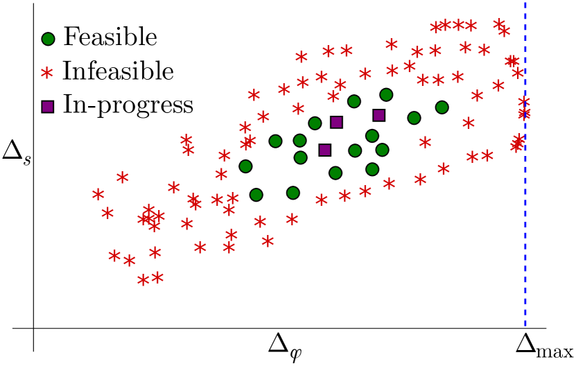
Figure 1: The max coordinates $\Delta_{\max}$ for a collection of allowed, disallowed, and in-progress points.

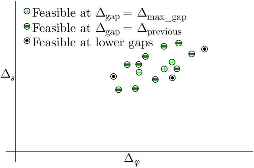
Figure 2: Different types of allowed points. Only the points allowed at $\Delta_{\text{gap}}=\Delta_{\text{previous}}$ are used for rescaling.

For a given $\Delta_{\text{allowed}}$, we define $\Delta_{\text{previous}}$ as the largest gap with allowed points but less than $\Delta_{\text{allowed}}$. This is usually a previous value for $\Delta_{\text{allowed}}$. Figure 2 shows an example of allowed points at $\Delta_{\text{allowed}}$, $\Delta_{\text{previous}}$, and lower gaps.

Using the $m$ allowed points at $\Delta_{\text{previous}}$, we scale the points using a principle component analysis. Specifically, we construct the matrix

$$M=\left(\begin{array}[]{cc}\Delta_{\phi 0}&\Delta_{s0}\\ \Delta_{\phi 1}&\Delta_{s1}\\ \Delta_{\phi 2}&\Delta_{s2}\\ \Delta_{\phi 3}&\Delta_{s3}\\ \vdots&\vdots\end{array}\right)\,.$$

We then compute the singular value decomposition (SVD) of this matrix

$$M=U\Sigma V^{*}\,,$$ (17)

where $\Sigma$ is a rectangular $m\times{N}$ diagonal matrix with non-negative real numbers $\sigma_{i}=\Sigma_{ii}$ on the diagonal ranging from the smallest ($\sigma_{\min}$) to the largest ($\sigma_{\max}$). $U$ is an $m\times m$ unitary matrix, and $V$ is an $N\times N$ (here $2\times 2$) unitary matrix.

We define the $N\times N$ matrix $\Omega$ as the first $N$ rows of $\Sigma$. This is a diagonal matrix with the entries $\sigma_{i}$, so the inverse is trivial. Putting this all together, we define the rescaling matrix

$$R\equiv\sigma_{\min}\Omega^{-1}V^{T}/\left(1.75\times\Delta_{\max}\right)\,.$$ (18)

It may be that there are so few points at $\Delta_{\text{previous}}$ that they are not linearly independent. For example, in the beginning, there may not be any points at $\Delta_{\text{previous}}$. If the ratio between the smallest ($\sigma_{\min}$) and largest ($\sigma_{\max}$) of these singular values is less than a tolerance (we use $10^{-8}$), then we only scale by $\Delta_{\max}$

$$R\equiv I/\left(1.75\times\Delta_{\max}\right)\,,$$ (19)

where $I$ is the identity.

Everything is scaled by the largest coordinate value $\Delta_{\max}$ to guarantee that all points are mapped into a box with extents (-1,1) in every dimension. The factor of 1.75 (about $\sqrt{3}$) is to ensure that all points will fit into the unit box even after rotation.

The transformation has the effect of a rotation and then rescaling of the rotated coordinates, so the allowed region remains convex. However, the allowed points should outline a more circular shape than the extended ellipse we started with, as shown in figure 4.

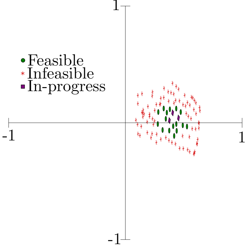
Figure 3: Points from figure 2 after rescaling.

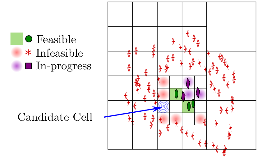
Figure 4: Points from figure 4 with an adapted mesh. Points that are allowed at $\Delta_{\text{gap}}<\Delta_{\text{allowed}}$ have been removed. The blue spiral indicates an empty candidate cell. The other empty cells are not diagonal from an allowed cell, so they are not considered.

One concern with this rescaling algorithm is that it weighs dense regions with more points more than equivalently sized regions with fewer points. So it may not produce an optimal transform. In practice, the later steps spread out the points very evenly, so this concern turns out not to be a problem in practice.

3.2.2 Adaptively meshing the box

While the distribution of points in figure 4 no longer has extreme aspect ratios, the points are still clustered in a small region of the unit box.

Based on the assumption that the allowed island only shrinks as the gap increases, we now only consider three sets of points: allowed at the current $\Delta_{\text{allowed}}$, disallowed at $\Delta_{\text{gap}}\leq\Delta_{\text{allowed}}$, and in-progress. For the rest of this step, we will be treating in-progress and disallowed points identically.

The strategy is to place points in regions that are empty. To quantify this emptiness, we create a hierarchy of meshes covering all the points. Empty regions are then cells that have no points.

The mesh hierarchy starts with a single coarse cell covering the entire unit box. The next level has $2^{N}$ cells (4 for our example), the level after that has $2^{2N}$ cells, and so on. This subdivision continues up to our predefined limit of 47 levels. This implies a relative minimum cell width of $2^{-47}$. This is quite small, but still significantly larger than the minimum resolution of an IEEE-754 double-precision number ($2^{-53}$). This helps reduce errors as points get rotated and scaled.

Next, we compute the coordinate extents of the allowed points in the transformed frame. For example, the extents in the transformed horizontal direction is the difference between the smallest and largest horizontal coordinates for the allowed points. This gives us a list of $N$ numbers. In figure 4, these extents are about 0.2 in both vertical and horizontal directions.

We then define a minimum cell size as the minimum of these $N$ extents multiplied by a fixed fraction $f_{\text{cutoff}}$. We use $f_{\text{cutoff}}=2$, which is deliberately very coarse. This tends to double the size of the allowed region at each step. Also, if $f_{\text{cutoff}}$ is too small, then the algorithm will completely fill in internal regions, even though, by assumption, the internal spaces do not need to be checked. This minimum cell size corresponds to a level $l_{\max}$ in the hierarchy of meshes.

Just after a jump to a higher gap, there is only one allowed point at $\Delta_{\text{allowed}}$. In this case, the extents are zero, so we set $l_{\max}=47$, the finest level.

Restricting our search to cells at level $l<l_{\max}$, we look for any empty cells adjacent to the allowed points. There will, in general, be multiple empty cells at multiple levels. We choose the largest empty cell.

If there are multiple candidates, we choose the cell adjacent to the first allowed point given to tiptop. So when driving tiptop, we always list the allowed points in the same order. If there are multiple candidates for a single point, then we select a new cell in the order

$$(+,+),(-,-),(+,-),(-,+).$$

We only check diagonals, so points get laid out in a checkerboard pattern as in figure 4.

The new point is not placed at the center of the new cell, but rather simply offset from the existing allowed point. So if the allowed point is in a corner of a cell, the new point will be in the same corner of the empty cell.

In practice, the implementation does not explicitly create the mesh at all levels. Rather, the points are stored in a tree. A node in the tree can have up to $2^{N}$ leaves, but leaves are only created if there is a point in that leaf. Adding a point to the tree adds it at all levels, so that it is easy to determine if a cell is occupied at any level.

The observed behavior of this algorithm is that it quickly finds a rough estimate for the boundary between allowed and disallowed, but can spend a lot of effort finding the exact boundaries. In-progress points are treated as disallowed, so too many in-progress points will lead to extra work. In practice, we have up to 16 points in-progress at any one time.

3.3 Jumping to a larger gap

If the previous section does not yield a new point, and there are no in-progress points at that gap, then we try to jump to a larger gap.

We start by rescaling the points as in section 3.2.1. We draw a coordinate box around all of the points allowed at $\Delta_{\text{allowed}}$ and shrink it by a factor of 2. Then we find the largest gap $\Delta_{\text{ceiling}}$ that can accommodate this box without containing any disallowed or in-progress points with $\Delta_{\text{gap}}\leq\Delta_{\text{ceiling}}$. At the beginning, there are no disallowed points at large gaps, so $\Delta_{\text{ceiling}}=\Delta_{\text{max\_gap}}.$

Defining $\Delta_{\text{diff}}\equiv\Delta_{\text{ceiling}}-\Delta_{\text{allowed}}$, we return the center of the box at $\Delta_{\text{gap}}=\Delta_{\text{allowed}}+\Delta_{\text{diff}}/2,$ thus bisecting the range of allowed gaps. This underscores the need for a good estimate of $\Delta_{\text{max\_gap}}.$ If the estimate is too high, then the algorithm will recommend too many points that are far too large.

One thing to note is that when running with multiple in-progress points, each subsequent point will be at a smaller $\Delta_{\text{gap}}$. So if there are 3 points running concurrently, they will be placed at $\Delta_{\text{allowed}}+\Delta_{\text{diff}}/2$, $\Delta_{\text{allowed}}+\Delta_{\text{diff}}/4$, and $\Delta_{\text{allowed}}+\Delta_{\text{diff}}/8$. If the first point at $\Delta_{\text{allowed}}+\Delta_{\text{diff}}/2$ succeeds, then any effort towards verifyinig the latter two points will be wasted.

This partition procedure means that a rough estimate for the upper bound is $\Delta_{\text{ceiling}}.$ This assumes both that the island itself is convex and that the allowed region near the tip of the allowed region is convex, as in Figure 7.

Overall, we have found this approach to work reasonably well. More importantly, it is very robust. It is very easy to be too clever, resulting in odd failures.

4 Results

4.1 Dimension bounds with OPE scans

Next we present our conformal bootstrap island computed using SDPB [41, 42], along with its comparison with various Monte Carlo results. Computing the conformal bootstrap island requires scanning over the three operator dimensions $\{\Delta_{\phi},\Delta_{s},\Delta_{t}\}$ using the Delaunay search algorithm described in [5], and for each point using the “cutting surface” algorithm presented in [5] to decide if there exists an allowed point in the space of OPE coefficient ratios $\{\frac{\lambda_{sss}}{\lambda_{\phi\phi s}},\frac{\lambda_{tts}}{\lambda_{\phi\phi s}},\frac{\lambda_{\phi\phi t}}{\lambda_{\phi\phi s}},\frac{\lambda_{ttt}}{\lambda_{\phi\phi s}}\}$.

When computing the island we make the following assumptions about the spectrum unless stated otherwise. We assume that $\phi$, $s$, and $t$ are the only relevant operators in their respective symmetry representations, so that $\Delta_{\phi^{\prime},s^{\prime},t^{\prime}}\geq 3$. In addition, we assume that the leading rank-4 scalar has a dimension satisfying $\Delta_{t_{4}}\geq 2$. We assume an ${O}(3)$ current with $\Delta_{J}=2$ and stress tensor with $\Delta_{T}=3$, with coefficients satisfying the Ward identity constraints. We also impose a twist gap above them, as well as in all other sectors not mentioned above, of size $10^{-6}$.

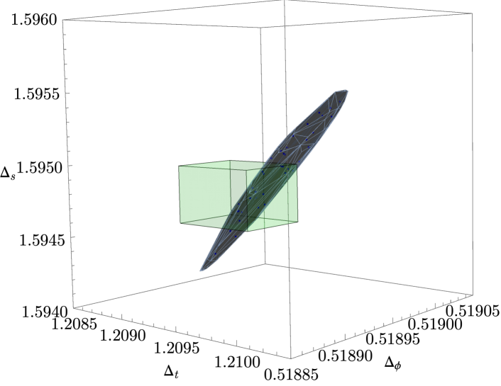
Figure 5: The $\Lambda=43$ conformal bootstrap dimension island (black) compared with the Monte Carlo results [7, 9] (green).

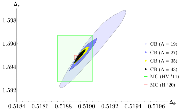
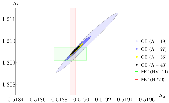
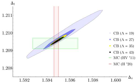
Figure 6: Comparison between the conformal bootstrap islands at $\Lambda=19,27,35,43$ projected to the $\{\Delta_{\phi},\Delta_{s}\}$, $\{\Delta_{\phi},\Delta_{t}\}$, and $\{\Delta_{s},\Delta_{t}\}$ planes and the Monte Carlo results of [7, 9].

In figure 5 we show the conformal bootstrap island we have computed at $\Lambda=43$ using these assumptions, compared to the Monte Carlo results of [7, 9]. In figure 6 we show various 2d projections of the bootstrap island. In appendix D we give the full set of allowed and disallowed points we computed at $\Lambda=43$, along with figure 9 which shows the convergence of the allowed points as a function of $\Lambda$ after performing an affine transformation to make the allowed regions roughly spherical.

In these plots we show our best determination of the allowed region at a given $\Lambda$, constructed by computing a Delaunay triangulation of the tested points, choosing triangles that contain both allowed and disallowed points, and plotting the convex hull of the points that are midway between the allowed and disallowed vertices in these triangles. At $\Lambda=43$, this “best-fit” region gives

$$\Delta_{\phi} =0.518942(51^{*})\,,$$

$$\Delta_{s} =1.59489(59^{*})\,,$$

$$\Delta_{t} =1.20954(23^{*})\,.$$ (20)

A more rigorous determination can be made by taking the convex hull of the disallowed points in these boundary Delaunay triangles. This region gives the rigorous error bars

$$\Delta_{\phi} =0.518936({\bf 67})\,,$$ (21)

$$\Delta_{s} =1.59488({\bf 81})\,,$$ (22)

$$\Delta_{t} =1.20954({\bf 32})\,,$$ (23)

which we have quoted in table 1.

The allowed points at $\Lambda=43$ are associated with OPE coefficient ratios which live in the ranges

$$\frac{\lambda_{sss}}{\lambda_{\phi\phi s}} =0.9643(20^{*})\,,$$

$$\frac{\lambda_{tts}}{\lambda_{\phi\phi s}} =1.87593(53^{*})\,,$$

$$\frac{\lambda_{\phi\phi t}}{\lambda_{\phi\phi s}} =1.66808(23^{*})\,,$$

$$\frac{\lambda_{ttt}}{\lambda_{\phi\phi s}} =2.86034(61^{*})\,.$$ (24)

These should be viewed as an approximation to the full allowed region of OPE coefficients, which may be slightly larger.

4.2 Central charges and $\lambda_{\phi\phi s}$

Next, we compute upper and lower bounds on the magnitude of the OPE coefficient $\lambda_{\phi\phi s}$, the central charge $C_{T}$, and the current central charge $C_{J}$. We compute these bounds over a small sample of points in our allowed region so the results will be inherently non-rigorous. However, we believe that this treatment gives reasonable estimates for these quantities that are more precise than previous results.

The strategy is similar to the method we employed in [5]. We take seven primal points in the $\Lambda=43$ island, consisting of the scaling dimensions and allowed OPE coefficients. The points are chosen to be sufficiently symmetrized and sparse across the $\Lambda=43$ island we have computed. For each of these points, we extremize $C_{T}$, $C_{J}$, and the external OPE norm parameterized by $\lambda_{\phi\phi s}$, to obtain upper and lower bounds. This calculation was limited to $\Lambda=35$ due to our available computational resources. The data points and SDPB parameters we used are summarized in tables 8 and 5, respectively.

There is an important comment we want to make about the upper bound computation on $C_{T}$ and $C_{J}$ (a similar comment was made in [5]). For computing upper bounds on $C_{T}$ and $C_{J}$, we have to assume a gap $\Delta_{T^{\prime}/J^{\prime}}$ above the unitarity bound for the next operators in the $T$ or $J$ sectors. Note that this gap was not assumed in our OPE scan, so this extra constraint might turn an allowed point into a disallowed point. If we do not have such a gap, the upper bound is loose and may not give reasonable results. On the other hand, large gaps can make SDPB unable to find a solution.

In table 8, we summarize the gaps $\Delta_{T^{\prime}/J^{\prime}}$ we assume in the upper bound calculations. From spectrum determinations using the extremal functional method (see [43, 44]), we have noticed that a gap $\Delta_{T^{\prime}/J^{\prime}}=\Delta_{T/J}+1$ above $T$ and $J$ is generally favored. We were able to compute bounds with this gap for three of the points, but for the other four we could not find solutions. For those points, we adopted the weaker assumption $\Delta_{\text{ext},T(J)}=\Delta_{T/J}+0.1$.

Following this procedure, we obtain our estimates of $C_{T}$, $C_{J}$, and $\lambda_{\phi\phi s}$ in the critical ${O}(3)$ model,

$${C_{J}}/C_{J}^{{\rm{free}}}={\rm{0.90632(}}{{\rm{16}}^{*}}{\rm{)}}\,,$$

$${C_{T}}/C_{T}^{{\rm{free}}}={\rm{0.944524(}}{{\rm{28}}^{*}}{\rm{)}}\,,$$

$${\lambda_{\phi\phi s}}={\rm{0.524261(}}{{\rm{59}}^{*}}{\rm{)}}\,.$$ (25)

These results agree with and are more precise than previous determinations of these quantitites (see [30, 10, 8]).

4.3 Upper bound on $\Delta_{t_{4}}$

Our last result is the maximum value of the rank-4 scalar dimension $\Delta_{t_{4}}$. In conjunction with the tiptop algorithm described in section 3, we computed points at $\Lambda=19,$ $27,$ and $35$. Allowed points at lower values of $\Lambda$ were used to initiate the search at larger values of $\Lambda$. Figure 7 shows a projection of a subset of the 1311 disallowed points and 172 allowed points at $\Lambda=35$, and Figure 8 shows how the island shrinks as we approach the maximum $\Delta_{t_{4}}$.

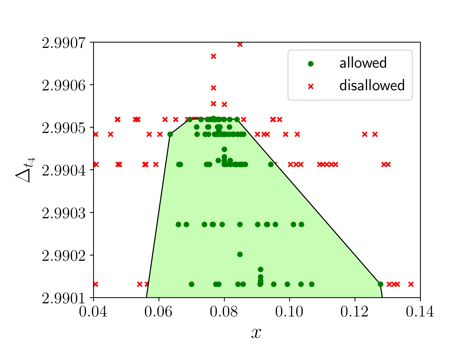
Figure 7: Two-dimensional projection of the results of the tiptop search at $\Lambda=35$. The $x$ coordinate is related to the three scalar dimensions via (D). Projections in $y$ and $z$ look similar. We have superimposed a convex hull encompassing the allowed points on top, obscuring some of the disallowed points. We can see the behaviour of the tiptop algorithm, exploring the island at one $\Delta_{t_{4}}$ before jumping to a larger $\Delta_{t_{4}}$. The jumps become progressively smaller, indicating convergence. We computed 16 points simultaneously, and this calculation took several months during which the tiptop algorithm was being developed. So the points reflect occasional crashes and small inefficiencies in the set of computed points.

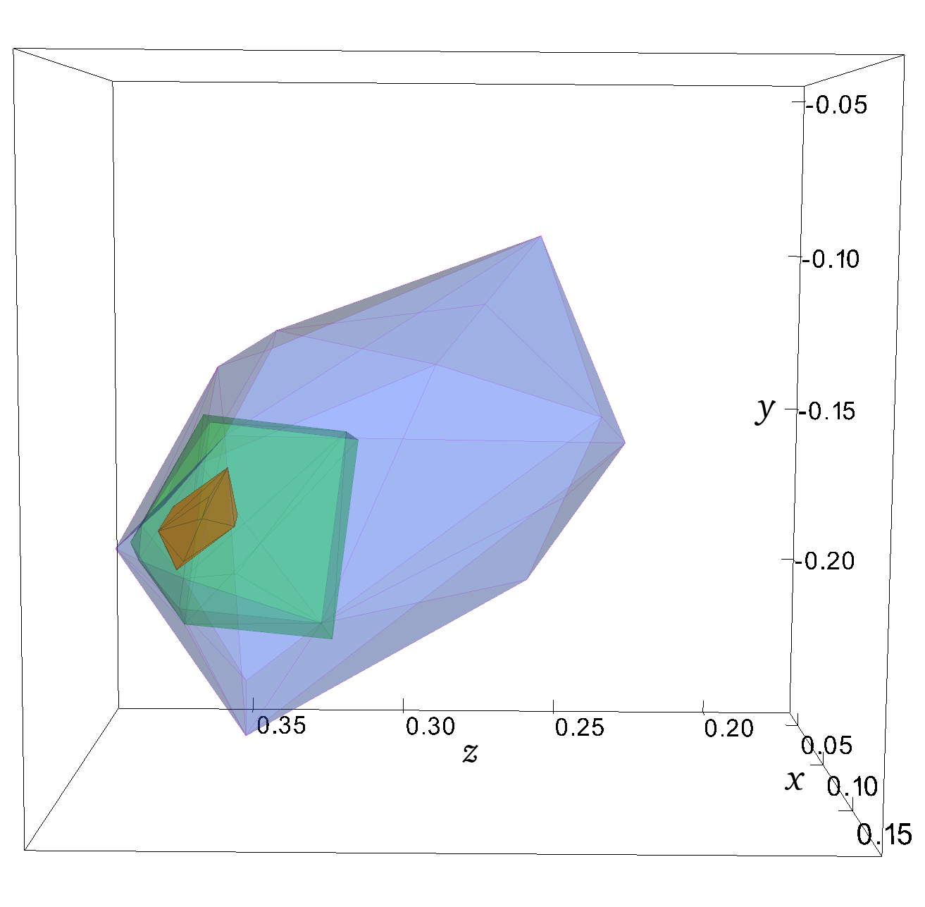
Figure 8: Three-dimensional islands of allowed points at different $\Delta_{t_{4}}$ at $\Lambda=35$, demonstrating how the islands shrink as we approach the maximum $\Delta_{t_{4}}$. The $x$, $y$, and $z$ coordinates are related to the three scalar dimensions via (D). The values for $\Delta_{t_{4}},$ from the largest region to smallest, are $2.989$, $2.99025$, and $2.9905$, with smaller values including all allowed points at larger values.

The largest allowed value of $\Delta_{t_{4}}$ was a single point at $2.99052$ with the scaling dimensions $\{\Delta_{\phi},\Delta_{s},\Delta_{t}\}=\{0.518962,1.59527,1.20969\}$. The limit from $\Delta_{\text{ceiling}}$ (see Section 3.3) is

$$\Delta_{t_{4}}<2.99056\,.$$ (26)

This implies that the leading rank-4 tensor in the critical ${O}(3)$ model is relevant, in agreement with other studies.

5 Future directions

In this work we have applied the methods developed in [5, 6] for large-scale bootstrap problems to the critical ${O}(3)$ model in three dimensions. This has led to results for scaling dimensions which are competitive with the most precise Monte Carlo simulations, and results for OPE coefficients which are significantly more precise than previous determinations. In addition, we have computed a rigorous bound on the scaling dimension of the leading rank-4 tensor, showing that it is relevant. Thus, any ${O}(3)$ system with cubic anisotropy should flow to the cubic fixed point (discussed in section 1.1.1) instead of the Heisenberg fixed point.

An interesting direction for future research will be the application of conformal perturbation theory to this flow. The cubic model can be reached by perturbing the ${O}(3)$ CFT with the operator $X\equiv\sum_{i=1}^{3}t_{4}^{iiii}$, which breaks ${O}(3)$ symmetry to the discrete symmetry $\mathds{Z}_{3}\rtimes\mathcal{S}_{3}$. From the ${O}(3)$ point of view, this term is a certain component of the ${O}(3)$ rank-4 tensor with dimension $\Delta_{t_{4}}\simeq 2.99$. On the other hand, in the cubic fixed point conformal perturbation theory predicts $\Delta_{X}\simeq 3.01$. Because this term is marginally irrelevant with $\delta=\Delta_{X}-3\simeq 0.01$, if we want to reach the cubic fixed point by a Monte Carlo simulation, the size of the lattice has to be around the order of $2^{1/\delta}$, which is impractical to implement.

An alternative way to estimate the cubic CFT data is using conformal perturbation theory. We start with the perturbed action $S=S_{{O}(3)}+g\int d^{3}xX$. Using the formalism in [45], one finds the beta function to be

$$\beta_{g}=-\delta g-\frac{\mathrm{vol}\,S^{d-1}}{2}\lambda_{XXX}g^{2}.$$ (27)

The dimension of an operator $\mathcal{O}$ at the cubic fixed point is then given at linear order in $\delta$ by $\Delta_{\mathcal{O}}=\Delta_{0}+2\delta\lambda_{\mathcal{O}\mathcal{O}X}/\lambda_{XXX}$, where $\Delta_{0}$ is the dimension of corresponding operator in the ${O}(3)$ CFT. Specifically one obtains $\Delta_{X}=\Delta_{0}+2\delta$, which justifies the estimate $\Delta_{X}\simeq 3.01$.

The OPE coefficient $\lambda_{XXX}$ is proportional to $\lambda_{t_{4}t_{4}t_{4}}$. Unfortunately, using the setup of the present paper, we don’t have access to $\lambda_{t_{4}t_{4}t_{4}}$. To access $\lambda_{t_{4}t_{4}t_{4}}$, one needs to bootstrap all four-point functions involving $\{\phi,s,t,t_{4}\}$, which is a concrete task for future research. Here we can estimate that the correction to $\Delta_{t}$ in the cubic fixed-point is of order $\delta=0.01$. On the other hand, the corrections to $\Delta_{\phi},\Delta_{s}$ start at order $\delta^{2}\simeq 0.0001$ since $\lambda_{\phi\phi t_{4}}=\lambda_{sst_{4}}=0$. Note that in this work the error bar for $\Delta_{t}$ is much smaller than $\delta$. Therefore a careful study of the $\{\phi,s,t,t_{4}\}$ system should yield a solid prediction for the correction to $\Delta_{t}$ in the cubic model.

Of course, it will also be interesting to understand how to isolate the cubic fixed point more directly using the conformal bootstrap, perhaps using a larger system of correlators than was considered in [31, 33, 34]. One can also straightforwardly apply the large-scale bootstrap techniques we have developed to other ${O}(N)$ models, as well as to 3d CFTs with fermions (using the newly developed software [46]) or to study conserved currents [47, 48, 49]. Using these methods one can also continue exploring larger systems of correlators that may help us to isolate CFTs containing gauge fields, such as 3d QED [50, 51] and 4d QCD.

Now that we have precisely isolated the ${O}(3)$ model, we are also in position to do a more detailed study of its low-twist trajectories of operators as a function of spin, which can be compared to analytical calculations using the Lorentzian Inversion formula [52, 53], following the approach of [54, 6, 55]. Such analytical techniques can also be used to estimate the leading Regge intercepts and related Lorentzian data of the ${O}(3)$ model. In future work it will also be important to understand how to better incorporate insights from the analytical bootstrap, such as our precise understanding of the large spin asymptotics, into making large-scale numerical methods even more powerful.

Appendix A Code availability

All code used in this work is available online. This includes the various codes described in appendix A of [5], as well as tiptop, available at https://gitlab.com/bootstrapcollaboration/tiptop. tiptop is implemented in C++17 and uses the Boost [56], Eigen [57], and VTK [58] libraries. The version used in this paper has the Git commit hash

• 23774017b8726699bd838cf138a65e29405f0907

Appendix B Software setup and parameters

The computations of the ${O}(3)$ model islands described in section 4.1 with $\Lambda=19,27$ were performed on the Caltech HPC Cluster, the Yale Grace Cluster, and the EPFL SCITAS cluster. For the computations with $\Lambda=35,43$, we tested possible primal points using the Caltech and Yale clusters. After finding a few initial primal points, the main Delaunay triangulation search was performed on the XSEDE Comet Cluster [59] at the San Diego Supercomputing Center through allocation PHY190023. Together, the computations of the $\Lambda=35$ island, the $\Lambda=43$ island, and the $\Lambda=35$ tiptop search took 2.94M CPU hours on the Comet Cluster. The optimization computations of section 4.2 were performed at $\Lambda=35$ and completed on the Caltech and Yale clusters.

We used the following choices for the set of spins at each value of $\Lambda$:

$$S_{19} =\{0,\dots,26\}\cup\{49,50\}\,,$$

$$S_{27} =\{0,\dots,31\}\cup\{49,50\}\,,$$

$$S_{35} =\{0,\dots,44\}\cup\{47,48,51,52,55,56,59,60,63,64,67,68\}\,,$$

$$S_{43} =\{0,\dots,64\}\cup\{67,68,71,72,75,76,79,80,83,84,87,88\}\,.$$ (28)

The SDPB parameters used in our computations are given in tables 4 and 5.

$\Lambda$	19	27	35	43
keptPoleOrder	14	14	32	40
order	60	60	80	90
spins	$S_{19}$	$S_{27}$	$S_{35}$	$S_{43}$
precision	768	768	960	1024
dualityGapThreshold	$10^{-30}$	$10^{-30}$	$10^{-30}$	$10^{-75}$
primalErrorThreshold	$10^{-200}$	$10^{-200}$	$10^{-200}$	$10^{-200}$
dualErrorThreshold	$10^{-200}$	$10^{-200}$	$10^{-200}$	$10^{-200}$
initialMatrixScalePrimal	$10^{40}$	$10^{50}$	$10^{50}$	$10^{60}$
initialMatrixScaleDual	$10^{40}$	$10^{50}$	$10^{50}$	$10^{60}$
feasibleCenteringParameter	0.1	0.1	0.1	0.1
infeasibleCenteringParameter	0.3	0.3	0.3	0.3
stepLengthReduction	0.7	0.7	0.7	0.7
maxComplementarity	$10^{100}$	$10^{130}$	$10^{160}$	$10^{200}$

Table 4: Parameters used for the computations of the conformal bootstrap islands in section 4.1. The sets $S_{\Lambda}$ are defined in (B).

$\Lambda$	35
keptPoleOrder	30
order	60
spins	$S_{35}$
precision	768
dualityGapThreshold	$10^{-20}$
primalErrorThreshold	$10^{-50}$
dualErrorThreshold	$10^{-60}$
initialMatrixScalePrimal	$10^{50}$
initialMatrixScaleDual	$10^{50}$
feasibleCenteringParameter	0.1
infeasibleCenteringParameter	0.3
stepLengthReduction	0.7
maxComplementarity	$10^{160}$

Table 5: Parameters used for the optimization computations in section 4.2. The set $S_{35}$ is defined in (B).

Appendix C Tensor structures

In this appendix we compute the ${SO}(3)$ tensor structures $T^{\mathcal{R}}$ that appear in the conformal block expansions (2.1) for the 4-point functions listed in table 3. We start by defining a basis of tensors for each configuration in table 3:

$$\begin{split}B_{\phi\phi\phi\phi}^{I}&=\begin{pmatrix}\delta_{ij}\delta_{kl}\\ \delta_{ik}\delta_{jl}\\ \delta_{il}\delta_{jk}\end{pmatrix}\,,\\ B^{I}_{tttt}&=\begin{pmatrix}\delta_{i_{1}j_{1}}\delta_{i_{2}j_{2}}\delta_{k_{1}l_{1}}\delta_{k_{2}l_{2}}\\ \delta_{i_{1}k_{1}}\delta_{i_{2}k_{2}}\delta_{j_{1}l_{1}}\delta_{j_{2}l_{2}}\\ \delta_{i_{1}l_{1}}\delta_{i_{2}l_{2}}\delta_{k_{1}j_{1}}\delta_{k_{2}j_{2}}\\ \delta_{i_{1}j_{1}}\delta_{i_{2}k_{2}}\delta_{k_{1}l_{1}}\delta_{j_{2}l_{2}}\\ \delta_{i_{1}j_{1}}\delta_{i_{2}l_{1}}\delta_{j_{2}k_{1}}\delta_{k_{2}l_{2}}\end{pmatrix}\,,\\ B_{t\phi t\phi}^{I}&=\begin{pmatrix}\delta_{i_{1}k_{1}}\delta_{i_{2}k_{2}}\delta_{j_{1}l_{1}}\\ \delta_{i_{1}j_{1}}\delta_{i_{2}k_{2}}\delta_{k_{1}l_{1}}\\ \delta_{i_{1}l_{1}}\delta_{i_{2}k_{2}}\delta_{j_{1}k_{1}}\end{pmatrix}\,,\\ B_{tt\phi\phi}^{I}&=\begin{pmatrix}\delta_{i_{1}j_{1}}\delta_{i_{2}j_{2}}\delta_{k_{1}l_{1}}\\ \delta_{i_{1}k_{1}}\delta_{i_{2}j_{2}}\delta_{j_{1}l_{1}}\\ \delta_{i_{1}l_{1}}\delta_{i_{2}j_{2}}\delta_{k_{1}j_{1}}\end{pmatrix}\,,\\ B_{ssss}&=1\,,\\ B_{\phi s\phi s}&=\delta_{ik}\,,\\ B_{tsts}&=\delta_{i_{1}k_{1}}\delta_{i_{2}k_{2}}\,,\\ B_{ttss}&=\delta_{i_{1}j_{1}}\delta_{i_{2}j_{2}}\,,\\ B_{\phi\phi ss}&=\delta_{ij}\,,\\ B_{\phi s\phi t}&=\delta_{il_{1}}\delta_{kl_{2}}\,,\\ B_{\phi\phi st}&=\delta_{il_{1}}\delta_{jl_{2}}\,,\\ B_{sttt}&=\delta_{j_{1}k_{1}}\delta_{j_{2}l_{1}}\delta_{k_{2}l_{2}}\,,\\ \end{split}$$ (29)

where the indices for each of the four operators are labeled as $i,j,k,l$ respectively, all indices with the same letter should be symmetrized with the trace removed, and for simplicity we suppress the indices on the left-hand side. For the first four configurations with non-trivial bases, we can find the tensor structure using the rank-2 ${SO}(3)$ Casimir $C$ acting on a basis $B$ with $n,m$ number of $i,j$ indices, respectively, as:

$$\begin{split}CB^{I}=\sum_{J}M^{IJ}B^{J}\,,\qquad C\equiv(G_{i_{1}^{\prime}}^{i_{1}}\oplus\dots\oplus G_{i_{n}^{\prime}}^{i_{n}}\oplus G_{j_{1}^{\prime}}^{j_{1}}\oplus\dots\oplus G_{j_{m}^{\prime}}^{j_{m}})^{2}\,,\end{split}$$ (30)

where $G$ are the usual ${SO}(3)$ generators. The $K$ eigenvectors $(T_{K})^{J}$ of $M^{IJ}$ are eigenvectors of $C$:

$$\begin{split}(CT_{K})^{I}=\sum_{J}M^{IJ}(T_{K})^{J}=c_{K}(T_{K})^{I}\,,\end{split}$$ (31)

where the eigenvalue $c$ for a rank $q$ ${SO}(3)$ irrep is $q(q+1)$, which allows us to identify each $T_{K}$ with an irrep. Up to an overall normalization, these $T_{K}$ are then the desired tensor structures. For the last 8 configurations there is only one basis element, so the tensor structure is simply that element also up to an overall normalization. The final list of tensor structures is then

$$\begin{split}\langle\phi\phi\phi\phi\rangle&:\qquad T^{\bf 0^{+}}_{\bf 1^{-}\bf 1^{-}\bf 1^{-}\bf 1^{-}}=B^{1}_{\phi\phi\phi\phi}\,,\\ &\qquad\;\;\;T^{\bf 1^{+}}_{\bf 1^{-}\bf 1^{-}\bf 1^{-}\bf 1^{-}}=B^{2}_{\phi\phi\phi\phi}-B^{3}_{\phi\phi\phi\phi}\,,\\ &\qquad\;\;\;T^{\bf 2^{+}}_{\bf 1^{-}\bf 1^{-}\bf 1^{-}\bf 1^{-}}=B^{2}_{\phi\phi\phi\phi}+B^{3}_{\phi\phi\phi\phi}-\frac{2}{3}B^{1}_{\phi\phi\phi\phi}\,,\\ \langle tttt\rangle&:\qquad T^{\bf 0^{+}}_{\bf 2^{+}\bf 2^{+}\bf 2^{+}\bf 2^{+}}=B^{1}_{tttt}\,,\\ &\qquad\;\;\;T^{\bf 1^{+}}_{\bf 2^{+}\bf 2^{+}\bf 2^{+}\bf 2^{+}}=B^{4}_{tttt}-B^{5}_{tttt}\,,\\ &\qquad\;\;\;T^{\bf 2^{+}}_{\bf 2^{+}\bf 2^{+}\bf 2^{+}\bf 2^{+}}=B^{4}_{tttt}+B^{5}_{tttt}-\frac{2}{3}B^{1}_{tttt}\,,\\ &\qquad\;\;\;T^{\bf 3^{+}}_{\bf 2^{+}\bf 2^{+}\bf 2^{+}\bf 2^{+}}=B^{5}_{tttt}-B^{4}_{tttt}-\frac{5}{4}B^{3}_{tttt}+\frac{5}{4}B^{2}_{tttt}\,,\\ &\qquad\;\;\;T^{\bf 4^{+}}_{\bf 2^{+}\bf 2^{+}\bf 2^{+}\bf 2^{+}}=-B^{5}_{tttt}-B^{4}_{tttt}+\frac{7}{12}B^{3}_{tttt}+\frac{7}{12}B^{2}_{tttt}+\frac{13}{30}B^{1}_{tttt}\,,\\ \langle t\phi t\phi\rangle,\langle\phi tt\phi\rangle&:\qquad T^{\bf 1^{-}}_{\bf 2^{+}\bf 1^{-}\bf 2^{+}\bf 1^{-}}=2B^{2}_{t\phi t\phi}\,,\\ &\qquad\;\;\;T^{\bf 2^{-}}_{\bf 2^{+}\bf 1^{-}\bf 2^{+}\bf 1^{-}}=-4B^{1}_{t\phi t\phi}+2B^{2}_{t\phi t\phi}+4B^{3}_{t\phi t\phi}\,,\\ &\qquad\;\;\;T^{\bf 3^{-}}_{\bf 2^{+}\bf 1^{-}\bf 2^{+}\bf 1^{-}}=10B^{1}_{t\phi t\phi}-8B^{2}_{t\phi t\phi}+20B^{3}_{t\phi t\phi}\,,\\ \langle tt\phi\phi\rangle&:\qquad T^{\bf 0^{+}}_{\bf 2^{+}\bf 2^{+}\bf 1^{-}\bf 1^{-}}=B^{1}_{tt\phi\phi}\,,\\ &\qquad\;\;\;T^{\bf 1^{+}}_{\bf 2^{+}\bf 2^{+}\bf 1^{-}\bf 1^{-}}=B^{2}_{tt\phi\phi}-B^{3}_{tt\phi\phi}\,,\\ &\qquad\;\;\;T^{\bf 2^{+}}_{\bf 2^{+}\bf 2^{+}\bf 1^{-}\bf 1^{-}}=B^{2}_{tt\phi\phi}+B^{3}_{tt\phi\phi}-\frac{2}{3}B^{1}_{tt\phi\phi}\,,\\ \langle ssss\rangle&:\qquad T^{\bf 0^{+}}_{\bf 0^{+}\bf 0^{+}\bf 0^{+}\bf 0^{+}}=B_{ssss}\,,\\ \langle\phi s\phi s\rangle,\langle s\phi\phi s\rangle&:\qquad T^{\bf 1^{-}}_{\bf 1^{-}\bf 0^{+}\bf 1^{-}\bf 2^{+}}=B_{\phi s\phi s}\,,\\ \langle tsts\rangle,\langle stts\rangle&:\qquad T^{\bf 2^{+}}_{\bf 2^{+}\bf 0^{+}\bf 2^{+}\bf 0^{+}}=B_{tsts}\,,\\ \langle ttss\rangle&:\qquad T^{\bf 0^{+}}_{\bf 2^{+}\bf 2^{+}\bf 0^{+}\bf 0^{+}}=B_{ttss}\,,\\ \langle\phi\phi ss\rangle&:\qquad T^{\bf 0^{+}}_{\bf 1^{-}\bf 1^{-}\bf 0^{+}\bf 0^{+}}=B_{\phi\phi ss}\,,\\ \langle\phi s\phi t\rangle,\langle s\phi\phi t\rangle&:\qquad T^{\bf 1^{-}}_{\bf 1^{-}\bf 0^{+}\bf 1^{-}\bf 2^{+}}={\sqrt{2}}B_{\phi s\phi t}\,,\\ \langle\phi\phi st\rangle&:\qquad T^{\bf 2^{+}}_{\bf 1^{-}\bf 1^{-}\bf 0^{+}\bf 2^{+}}=\sqrt{2}B_{\phi\phi st}\,,\\ \langle sttt\rangle,\langle ttst\rangle&:\qquad T^{\bf 2^{+}}_{\bf 0^{+}\bf 2^{+}\bf 2^{+}\bf 2^{+}}=\sqrt{2}B_{sttt}\,.\\ \end{split}$$ (32)

The overall normalization of these tensor structures has been chosen so that the OPE coefficients $\lambda_{\varphi_{1}\varphi_{2}\mathcal{O}}$ and $\lambda_{\varphi_{3}\varphi_{4}\mathcal{O}}$ in (2.1) are consistent under permutation of their subscripts. This can be checked using the free theory, where we have the operators

$$\begin{split}s(x)\equiv\frac{1}{\sqrt{6}}\phi^{i}(x)\phi^{i}(x)\,,\qquad t^{ij}(x)\equiv\frac{1}{\sqrt{2}}\phi^{i}(x)\phi^{j}(x)-\mathrm{trace}\,,\end{split}$$ (33)

which have been normalized consistent with the 2-point function normalization in (13). We can then compute all the 4-point functions in table 3 using Wick contractions and expand in blocks as in (2.1) using the tensor structures in (32) to verify this consistency.

Appendix D Computed points

In table 6 we list the 38 primal points we have computed in the $\Lambda=43$ island and in table 7 we list the 270 dual points we computed at $\Lambda=43$. In table 8 we list the 7 primal points we use for the optimization computations described in section 4.2.

In figure 9 we show a plot of the allowed regions at $\Lambda=19,27,35,43$ after performing an affine transformation which makes the $\Lambda=19$ region roughly spherical. The precise affine transformation is given by:

$$x =228.67-107.177\Delta_{s}-43.8661\Delta_{t}-8.77302\Delta_{\phi}\,,$$

$$y =-1061.39-694.406\Delta_{s}+1612.44\Delta_{t}+420.885\Delta_{\phi}\,,$$ (35)

$$z =2590.87-221.685\Delta_{s}+2629.52\Delta_{t}-10439.6\Delta_{\phi}\,.$$

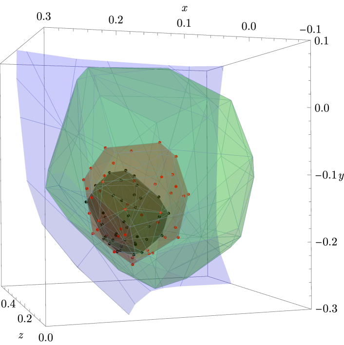
Figure 9: The convex hulls of the allowed points in the affine space (D) at derivative orders $\Lambda=19,27,35,43$. The red and black data points are the allowed points at derivative orders $\Lambda=35,43$.

$\Delta_{\phi}$	$\Delta_{s}$	$\Delta_{t}$	$\frac{{\lambda_{sss}}}{\lambda_{\phi\phi s}}$	$\frac{{\lambda_{tts}}}{\lambda_{\phi\phi s}}$	$\frac{{\lambda_{\phi\phi t}}}{\lambda_{\phi\phi s}}$	$\frac{{\lambda_{ttt}}}{\lambda_{\phi\phi s}}$
0.5189783882	1.5953612741	1.2097311776	0.9658557781	1.8764272526	1.6683150562	2.8608280295
0.5189583670	1.5949959168	1.2096121876	0.9637866930	1.8759071995	1.6681321958	2.8604010933
0.5189461401	1.5949711389	1.2095536502	0.9650503920	1.8758868056	1.6680723076	2.8601976693
0.5189272852	1.5948074081	1.2094888929	0.9652812111	1.8758487781	1.6680235398	2.8603061675
0.5189613339	1.5952564268	1.2096662222	0.9662461846	1.8763712143	1.6682528867	2.8607475247
0.5189198114	1.5946719225	1.2094285955	0.9639220579	1.8755694851	1.6679344313	2.8599409571
0.5189172850	1.5946165394	1.2094312995	0.9634877179	1.8756194443	1.6679524398	2.8599835329
0.5189500473	1.5951798121	1.2096307308	0.9661780974	1.8763286685	1.6682360908	2.8607267382
0.5189649901	1.5951958587	1.2096821376	0.9647455098	1.8763265571	1.6682560921	2.8608385887
0.5189431822	1.5950799657	1.2095793546	0.9658559545	1.8761787760	1.6681550694	2.8604066434
0.5189526027	1.5949370220	1.2096034154	0.9633651701	1.8758925982	1.6681462865	2.8605568949
0.5189301757	1.5949315300	1.2095370407	0.9653175705	1.8761152596	1.6681181238	2.8605816730
0.5189168372	1.5946844827	1.2094296026	0.9642949506	1.8756631385	1.6679573604	2.8599418324
0.5189483062	1.5950509260	1.2095711164	0.9654214538	1.8760347497	1.6681115766	2.8602582414
0.5189153515	1.5946825124	1.2094352034	0.9643765341	1.8757126829	1.6679642216	2.8601068005
0.5189440155	1.5949715807	1.2095885922	0.9644538043	1.8760784038	1.6681817119	2.8607365030
0.5189150284	1.5945099455	1.2094139921	0.9622684128	1.8754680443	1.6679176085	2.8599290431
0.5189347282	1.5947841912	1.2094914029	0.9639498317	1.8756547299	1.6679896459	2.8599829650
0.5189802791	1.5952998277	1.2097251950	0.9649312284	1.8762516023	1.6682831892	2.8609105511
0.5189248611	1.5948368279	1.2094835818	0.9649249785	1.8759055628	1.6680304724	2.8600899846
0.5189306747	1.5946954535	1.2094799696	0.9630209667	1.8756016368	1.6679818979	2.8600556364
0.5189217812	1.5947698290	1.2094894198	0.9646493947	1.8759369337	1.6680732162	2.8603682382
0.5189121284	1.5945494559	1.2093932170	0.9632128469	1.8754599512	1.6678971836	2.8597295069
0.5189738261	1.5953116389	1.2096932265	0.9658322350	1.8762663003	1.6682491526	2.8606277206
0.5189145348	1.5947341024	1.2094532479	0.9650247104	1.8759430722	1.6680183536	2.8602402387
0.5189014384	1.5944048949	1.2093555400	0.9627737264	1.8753951336	1.6678520403	2.8597952050
0.5189305457	1.5947604700	1.2094652572	0.9640748832	1.8756103384	1.6679623986	2.8598809964
0.5189623990	1.5950949062	1.2096629593	0.9640070854	1.8761554772	1.6682313428	2.8608189553
0.5189460789	1.5950582403	1.2095808918	0.9654253734	1.8761261589	1.6681362224	2.8605045135
0.5189301505	1.5949452685	1.2095278745	0.9657542568	1.8760854806	1.6681017321	2.8604962327
0.5189685635	1.5953320391	1.2097096529	0.9660028358	1.8764583565	1.6683135549	2.8609575117
0.5189497511	1.5949209137	1.2095606097	0.9638109344	1.8758202300	1.6680711351	2.8601899822
0.5189337664	1.5947155621	1.2095107201	0.9623655424	1.8757184969	1.6680386790	2.8602450223
0.5189453714	1.5951023898	1.2096147301	0.9659065454	1.8763651079	1.6682206940	2.8607919521
0.5189862601	1.5954028918	1.2097515683	0.9654844905	1.8763339257	1.6683105873	2.8607881451
0.5189476979	1.5949533896	1.2096010827	0.9637175659	1.8760304271	1.6681861098	2.8606729585
0.5189346015	1.5950348003	1.2095678602	0.9659534043	1.8763062992	1.6681684361	2.8606248190
0.5189598320	1.5951484795	1.2096664021	0.9647455098	1.8763265571	1.6682560921	2.8608385887

Table 6: Allowed points in the $\Lambda=43$ island.

$\Delta_{\phi}$	$\Delta_{s}$	$\Delta_{t}$
0.5187966798	1.5921850401	1.2086228804
0.5189025751	1.5940361780	1.2092959408
0.5189114364	1.5946504985	1.2093872462
0.5189189599	1.5941920882	1.2093299741
0.5189288736	1.5938535802	1.2091078506
0.5186945881	1.5924442671	1.2084245865
0.5187373587	1.5921586352	1.2084312743
0.5187762022	1.5918820333	1.2086546805
0.5187826937	1.5914255278	1.2085310641
0.5188353864	1.5934222782	1.2090020249
0.5188362222	1.5935429810	1.2089818386
0.5188416799	1.5933781659	1.2089481869
0.5188478354	1.5938857812	1.2091362879
0.5188535569	1.5932852248	1.2088214042
0.5188541349	1.5932916366	1.2089652272
0.5188547707	1.5939362783	1.2090312421
0.5188571369	1.5930390946	1.2090569647
0.5188574085	1.5927203987	1.2089917699
0.5188612075	1.5939110280	1.2091455740
0.5188615055	1.5937167137	1.2090909898
0.5188768144	1.5938159784	1.2090216235
0.5188830465	1.5941282784	1.2092443533
0.5188846453	1.5942465723	1.2092589387
0.5188859294	1.5941864473	1.2092761662
0.5188862012	1.5941115729	1.2092255065
0.5188873828	1.5941812791	1.2092506161
0.5188874108	1.5939452740	1.2091859961
0.5188875107	1.5943066473	1.2093007022
0.5188888052	1.5938613363	1.2092121233
0.5188955343	1.5940894591	1.2092127567
0.5188965815	1.5941441764	1.2092975081
0.5189023610	1.5945285422	1.2093834019
0.5189038211	1.5934538031	1.2090700892
0.5189054986	1.5948072619	1.2094576026
0.5189068088	1.5944337603	1.2092909633
0.5189083086	1.5946728229	1.2094131489
0.5189105727	1.5946476632	1.2094486445
0.5189114164	1.5934097919	1.2091414652
0.5189153608	1.5942042741	1.2092982492
0.5189179786	1.5948735383	1.2094980056
0.5189191601	1.5945565549	1.2094640368
0.5189241090	1.5941509824	1.2094002783
0.5189333103	1.5939599259	1.2094523297
0.5189333930	1.5943501521	1.2094232463
0.5189346097	1.5944851028	1.2095740716
0.5189237305	1.5944279251	1.2093905391
0.5188043639	1.5926034786	1.2087905625
0.5188819788	1.5940503654	1.2091664050
0.5189348544	1.5939659673	1.2093605905
0.5189331311	1.5945586909	1.2094861373
0.5188609431	1.5938359757	1.2091138392
0.5189041783	1.5931200581	1.2091359461
0.5189211553	1.5940068208	1.2093711976
0.5188230608	1.5930667503	1.2087833097
0.5187918880	1.5920291631	1.2086556637
0.5187954081	1.5933857238	1.2088722712
0.5188120708	1.5921939042	1.2085475622
0.5188685720	1.5940780889	1.2092200213
0.5188737587	1.5938867482	1.2091282102
0.5188791085	1.5939475441	1.2092269843
0.5188860122	1.5944086593	1.2093118142
0.5188881256	1.5943425103	1.2092606077
0.5188962192	1.5944000610	1.2093036926
0.5188995836	1.5944714851	1.2093479909
0.5189042967	1.5942997732	1.2093450874
0.5189061160	1.5944245329	1.2093054811
0.5189130711	1.5943416289	1.2092938887
0.5189282439	1.5948696505	1.2094354495
0.5189381636	1.5945869176	1.2095373290
0.5189209582	1.5946145623	1.2093971026
0.5188528255	1.5932931016	1.2088647649
0.5188758367	1.5937600844	1.2090694206
0.5189034036	1.5943173907	1.2092753786
0.5187933545	1.5923524886	1.2085851052
0.5188028340	1.5925358527	1.2086181925
0.5188672706	1.5938859690	1.2090784902
0.5188721453	1.5939744974	1.2092114019
0.5188815521	1.5940429270	1.2090230925
0.5188876803	1.5938597752	1.2092439737
0.5188893843	1.5942285412	1.2092430003
0.5188959297	1.5932555635	1.2092613868
0.5189185378	1.5944533142	1.2093899362
0.5189206686	1.5947871150	1.2094529310
0.5189513139	1.5946586522	1.2094523424
0.5189385685	1.5946849443	1.2094603545
0.5189444575	1.5946106034	1.2094426944
0.5189597959	1.5951033035	1.2095684829
0.5190271291	1.5953552765	1.2099320047
0.5191718508	1.5977020194	1.2105467890
0.5189415400	1.5950976756	1.2095440010

$\Delta_{\phi}$	$\Delta_{s}$	$\Delta_{t}$
0.5189424979	1.5947703013	1.2093601723
0.5189461102	1.5944802637	1.2095417129
0.5189461142	1.5952505758	1.2096113811
0.5189509729	1.5951396676	1.2096608087
0.5189524992	1.5951035671	1.2095733650
0.5189561892	1.5950657026	1.2096530941
0.5189575751	1.5955030599	1.2096401327
0.5189576562	1.5952623581	1.2096851550
0.5189595475	1.5954833608	1.2097148970
0.5189682325	1.5951956784	1.2096321472
0.5189696503	1.5942534718	1.2093617878
0.5189733687	1.5949010519	1.2095786060
0.5189772029	1.5950953535	1.2096440413
0.5189800482	1.5949290496	1.2097035540
0.5189804744	1.5953372481	1.2097875328
0.5189818184	1.5960483373	1.2098711894
0.5189830613	1.5952764767	1.2098175729
0.5189871624	1.5963425034	1.2098915261
0.5189966010	1.5956243058	1.2098589501
0.5190066292	1.5959897652	1.2099481084
0.5190086343	1.5954797940	1.2098872690
0.5190093925	1.5948495201	1.2095311073
0.5190140405	1.5954232716	1.2098887955
0.5190158019	1.5958546312	1.2098800029
0.5190176624	1.5957396035	1.2099524800
0.5190182636	1.5952950369	1.2097197630
0.5190222887	1.5962382824	1.2100406599
0.5190294335	1.5944921267	1.2097386508
0.5190368914	1.5960448579	1.2099540543
0.5190379431	1.5958717009	1.2099655030
0.5190482917	1.5959534075	1.2099669869
0.5190587928	1.5959983074	1.2100169645
0.5190598740	1.5957892478	1.2100080216
0.5190647361	1.5962663027	1.2101521345
0.5190695509	1.5960823090	1.2101350323
0.5190725277	1.5960088046	1.2100991203
0.5190732657	1.5962258325	1.2100744510
0.5190787856	1.5961544869	1.2101199950
0.5190839387	1.5962931060	1.2101834489
0.5190846538	1.5964564464	1.2101823824
0.5190882951	1.5952923328	1.2099488238
0.5191014483	1.5962764902	1.2102433612
0.5191200121	1.5963878404	1.2104254692
0.5191238375	1.5961605267	1.2100960457
0.5191427139	1.5977670021	1.2106878967
0.5191456549	1.5971361619	1.2105308642
0.5191695884	1.5970766016	1.2106595054
0.5191747564	1.5961581015	1.2104165938
0.5191752118	1.5973305922	1.2104827329
0.5191772163	1.5979425702	1.2107834542
0.5191998406	1.5976763974	1.2108343370
0.5192110760	1.5974046747	1.2105784428
0.5192313582	1.5976397828	1.2109134929
0.5192577054	1.5985007420	1.2110602270
0.5192609179	1.5973050662	1.2108724994
0.5192751871	1.5986516951	1.2111693213
0.5193182009	1.5988546582	1.2112832624
0.5193313395	1.5984303509	1.2111533312
0.5193414850	1.5980461969	1.2111569121
0.5193551983	1.5998541317	1.2115697595
0.5193848130	1.5991038253	1.2114973135
0.5193945892	1.5989679837	1.2114217221
0.5190798632	1.5964346557	1.2102061791
0.5189741917	1.5955685395	1.2097697715
0.5189927891	1.5951952177	1.2097372791
0.5189996154	1.5950788378	1.2097054113
0.5190167890	1.5955602397	1.2098873787
0.5190308122	1.5949198011	1.2096389844
0.5190339170	1.5955996031	1.2098749137
0.5190412371	1.5962115376	1.2100681124
0.5191177942	1.5966893312	1.2103147962
0.5192445379	1.5985977149	1.2110282728
0.5192695593	1.5991098729	1.2112586408
0.5193036599	1.5986614215	1.2113279731
0.5192414561	1.5971357017	1.2106354701
0.5189651659	1.5950121240	1.2096667988
0.5191751265	1.5980350400	1.2107387866
0.5189584563	1.5953669776	1.2096954753
0.5189653470	1.5950297999	1.2096904832
0.5189699612	1.5955018495	1.2097342211
0.5189780238	1.5954734077	1.2097071812
0.5189801701	1.5956399491	1.2098195524
0.5189846429	1.5956222286	1.2098043739
0.5189848116	1.5942072297	1.2094316101
0.5189955714	1.5956904175	1.2098601902
0.5189970055	1.5958004005	1.2098315960
0.5190050996	1.5957883004	1.2098865696
0.5190163339	1.5957550559	1.2099183538
0.5190199557	1.5956651380	1.2099295296
0.5190607004	1.5962908080	1.2100873837

$\Delta_{\phi}$	$\Delta_{s}$	$\Delta_{t}$
0.5190663597	1.5958743309	1.2100957055
0.5190718073	1.5963854342	1.2101543103
0.5191015148	1.5964779979	1.2103173913
0.5191201873	1.5971879432	1.2103557329
0.5191327281	1.5966479322	1.2102157357
0.5192390608	1.5990575125	1.2111165018
0.5189384637	1.5945786868	1.2092964612
0.5189388374	1.5949295375	1.2094886518
0.5189406470	1.5951736959	1.2096025578
0.5189435236	1.5946628177	1.2095079568
0.5189591857	1.5937291370	1.2094479043
0.5189690300	1.5947953102	1.2095700139
0.5189782490	1.5955014573	1.2097394518
0.5189785861	1.5948000056	1.2096217602
0.5189943897	1.5951836165	1.2096726879
0.5190020000	1.5955721180	1.2098614948
0.5190031045	1.5956425756	1.2098293707
0.5190089551	1.5959677551	1.2099413822
0.5190264203	1.5960422185	1.2100190836
0.5190349642	1.5958180205	1.2099706558
0.5190621203	1.5957337543	1.2098389282
0.5191180161	1.5968444953	1.2103456280
0.5191470052	1.5962315204	1.2104571613
0.5191921249	1.5963777247	1.2105975545
0.5192666256	1.5975999519	1.2109769054
0.5192834446	1.5981834807	1.2109478678
0.5192153931	1.5971409678	1.2108619123
0.5190126129	1.5960328832	1.2098411820
0.5189956968	1.5952697384	1.2097891345
0.5190907117	1.5964405597	1.2102564468
0.5189972378	1.5954623091	1.2097288249
0.5192342602	1.5977739085	1.2106788412
0.5192967458	1.5978374167	1.2109654958
0.5190531962	1.5957547434	1.2100253487
0.5190597017	1.5959435763	1.2100960808
0.5189393710	1.5943081218	1.2094518082
0.5189538314	1.5947940605	1.2094896280
0.5189547388	1.5948394180	1.2095585036
0.5189639253	1.5945186785	1.2094725381
0.5189836057	1.5957551038	1.2098219526
0.5189905121	1.5953498417	1.2098007194
0.5189919017	1.5941900169	1.2095288310
0.5189979105	1.5956955072	1.2097796040
0.5189995667	1.5957402879	1.2099058216
0.5190123754	1.5941042932	1.2095390773
0.5190157406	1.5958569876	1.2099200545
0.5190278431	1.5965081852	1.2100281015
0.5190325131	1.5959081051	1.2099696538
0.5190520384	1.5963152404	1.2100841277
0.5190588609	1.5960509826	1.2099090548
0.5190715439	1.5955912797	1.2101497526
0.5190926525	1.5965090465	1.2102403519
0.5191170800	1.5974916154	1.2105064335
0.5191778676	1.5977308111	1.2107843923
0.5192544590	1.5971285489	1.2107746440
0.5192666631	1.5983714488	1.2109356823
0.5192812420	1.5987160882	1.2111101581
0.5193040795	1.5983604351	1.2112010479
0.5189685870	1.5947440353	1.2095546973
0.5189469362	1.5948003211	1.2094569896
0.5190500327	1.5959140301	1.2100673844
0.5190853457	1.5968203648	1.2103356646
0.5189402432	1.5947339426	1.2095132572
0.5189866072	1.5952602047	1.2097386461
0.5189466850	1.5949712041	1.2095439276
0.5189977538	1.5955819151	1.2098187686
0.5189417109	1.5948151822	1.2095116242
0.5189887395	1.5955311410	1.2097998738
0.5189805152	1.5954860043	1.2097574571
0.5189068037	1.5944354150	1.2093631340
0.5189664963	1.5953900793	1.2097088870
0.5189046136	1.5944739467	1.2093498390
0.5189477115	1.5951943364	1.2096143706
0.5189476015	1.5951048660	1.2095857135
0.5189392465	1.5947339121	1.2095257880
0.5189758138	1.5951810417	1.2097131902
0.5189281878	1.5946813688	1.2094996850
0.5189741332	1.5953607762	1.2097417847
0.5189225607	1.5945597787	1.2094380766
0.5189250556	1.5947901155	1.2094599723
0.5189931813	1.5954181855	1.2097690833
0.5189417323	1.5950007532	1.2095363269
0.5189436065	1.5950358588	1.2096059939
0.5189964571	1.5954554607	1.2098005401
0.5189717084	1.5953355582	1.2096832796
0.5189194848	1.5945704303	1.2094129825
0.5189261393	1.5947676104	1.2095065854
0.5189163665	1.5945874291	1.2093899278
0.5188888691	1.5942500939	1.2092859143
0.5189931888	1.5954995182	1.2097983737

Table 7: Disallowed points computed at $\Lambda=43$.

$\Delta_{\phi}$	$\Delta_{s}$	$\Delta_{t}$	$\frac{{\lambda_{sss}}}{\lambda_{\phi\phi s}}$	$\frac{{\lambda_{tts}}}{\lambda_{\phi\phi s}}$	$\frac{{\lambda_{\phi\phi t}}}{\lambda_{\phi\phi s}}$	$\frac{{\lambda_{ttt}}}{\lambda_{\phi\phi s}}$	$\Delta_{T^{\prime}}-\Delta_{T}$	$\Delta_{J^{\prime}}-\Delta_{J}$
0.5189121284	1.594549456	1.209393217	0.9632128469	1.875459951	1.667897184	2.859729507	1.0	0.1
0.5189145348	1.594734102	1.209453248	0.9650247103	1.875943072	1.668018354	2.860240239	1.0	1.0
0.5189337664	1.594715562	1.209510720	0.9623655424	1.875718497	1.668038679	2.860245022	1.0	1.0
0.5189415373	1.594941048	1.209557043	0.9646177852	1.875978443	1.668107872	2.860397307	1.0	1.0
0.5189431822	1.595079966	1.209579355	0.9658559545	1.876178776	1.668155069	2.860406643	1.0	0.1
0.5189685635	1.595332039	1.209709653	0.9660028358	1.876458357	1.668313555	2.860957512	1.0	0.1
0.5189862601	1.595402892	1.209751568	0.9654844905	1.876333926	1.668310587	2.860788145	1.0	0.1

Table 8: Allowed points in the $\Lambda=43$ island used to obtain bounds on $\lambda_{\phi\phi s}$, $C_{T}$, and $C_{J}$, along with the gaps above $\Delta_{T}$ and $\Delta_{J}$ that were assumed.

References

- [1] R. Rattazzi, V. S. Rychkov, E. Tonni, and A. Vichi, “Bounding scalar operator dimensions in 4D CFT,” JHEP 0812 (2008) 031, arXiv:0807.0004 [hep-th].
- [2] V. S. Rychkov and A. Vichi, “Universal Constraints on Conformal Operator Dimensions,” Phys.Rev. D80 (2009) 045006, arXiv:0905.2211 [hep-th].
- [3] D. Poland, S. Rychkov, and A. Vichi, “The Conformal Bootstrap: Theory, Numerical Techniques, and Applications,” Rev. Mod. Phys. 91 no. 1, (2019) 15002, arXiv:1805.04405 [hep-th]. [Rev. Mod. Phys.91,015002(2019)].
- [4] S. M. Chester, “Weizmann Lectures on the Numerical Conformal Bootstrap,” arXiv:1907.05147 [hep-th].
- [5] S. M. Chester, W. Landry, J. Liu, D. Poland, D. Simmons-Duffin, N. Su, and A. Vichi, “Carving out OPE space and precise model critical exponents,” JHEP 06 (2020) 142, arXiv:1912.03324 [hep-th].
- [6] J. Liu, D. Meltzer, D. Poland, and D. Simmons-Duffin, “The Lorentzian inversion formula and the spectrum of the 3d O(2) CFT,” JHEP 09 (2020) 115, arXiv:2007.07914 [hep-th].
- [7] M. Hasenbusch, “Monte Carlo study of a generalized icosahedral model on the simple cubic lattice,” Phys. Rev. B 102 no. 2, (2020) 024406, arXiv:2005.04448 [cond-mat.stat-mech].
- [8] F. Kos, D. Poland, D. Simmons-Duffin, and A. Vichi, “Precision Islands in the Ising and Models,” JHEP 08 (2016) 036, arXiv:1603.04436 [hep-th].
- [9] M. Hasenbusch and E. Vicari, “Anisotropic perturbations in three-dimensional o(n)-symmetric vector models,” Physical Review B 84 no. 12, (Sep, 2011) 125136. http://dx.doi.org/10.1103/PhysRevB.84.125136.
- [10] F. Kos, D. Poland, D. Simmons-Duffin, and A. Vichi, “Bootstrapping the O(N) Archipelago,” JHEP 11 (2015) 106, arXiv:1504.07997 [hep-th].
- [11] J. M. Carmona, A. Pelissetto, and E. Vicari, “The N component Ginzburg-Landau Hamiltonian with cubic anisotropy: A Six loop study,” Phys. Rev. B61 (2000) 15136–15151, arXiv:cond-mat/9912115 [cond-mat].
- [12] A. Aharony and M. E. Fisher, “Critical behavior of magnets with dipolar interactions. i. renormalization group near four dimensions,” Phys. Rev. B 8 (Oct, 1973) 3323–3341. https://link.aps.org/doi/10.1103/PhysRevB.8.3323.
- [13] D. R. Nelson, J. M. Kosterlitz, and M. E. Fisher, “Renormalization-group analysis of bicritical and tetracritical points,” Phys. Rev. Lett. 33 (Sep, 1974) 813–817. https://link.aps.org/doi/10.1103/PhysRevLett.33.813.
- [14] F. Jasch and H. Kleinert, “Fast-convergent resummation algorithm and critical exponents of phi4-theory in three dimensions,” Journal of Mathematical Physics 42 no. 1, (Jan, 2001) 52–73. http://dx.doi.org/10.1063/1.1289377.
- [15] R. Guida and J. Zinn-Justin, “Critical exponents of then-vector model,” Journal of Physics A: Mathematical and General 31 no. 40, (Oct, 1998) 8103–8121. http://dx.doi.org/10.1088/0305-4470/31/40/006.
- [16] P. Butera and M. Comi, “Renormalized couplings and scaling correction amplitudes in then-vector spin models on the sc and the bcc lattices,” Physical Review B 58 no. 17, (Nov, 1998) 11552–11569. http://dx.doi.org/10.1103/PhysRevB.58.11552.
- [17] P. Calabrese, A. Pelissetto, and E. Vicari, “Randomly dilute spin models with cubic symmetry,” Physical Review B 67 no. 2, (Jan, 2003) 024418. http://dx.doi.org/10.1103/PhysRevB.67.024418.
- [18] P. Pfeuty, D. Jasnow, and M. E. Fisher, “Crossover scaling functions for exchange anisotropy,” Phys. Rev. B 10 (Sep, 1974) 2088–2112. https://link.aps.org/doi/10.1103/PhysRevB.10.2088.
- [19] P. Calabrese, A. Pelissetto, and E. Vicari, “Critical structure factors of bilinear fields in o(n) vector models,” Physical Review E 65 no. 4, (Apr, 2002) 046115. http://dx.doi.org/10.1103/PhysRevE.65.046115.
- [20] H. Kleinert and V. Schulte-Frohlinde, “Exact five-loop renormalization group functions of -theory with o(n)-symmetric and cubic interactions. critical exponents up to ,” Physics Letters B 342 no. 1-4, (Jan, 1995) 284–296. http://dx.doi.org/10.1016/0370-2693(94)01377-O.
- [21] K. Varnashev, “Stability of a cubic fixed point in three-dimensions: Critical exponents for generic N,” Phys. Rev. B 61 (2000) 14660, arXiv:cond-mat/9909087.
- [22] R. Folk, Y. Holovatch, and T. Yavorskii, “Pseudo- expansion of six-loop renormalization-group functions of an anisotropic cubic model,” Physical Review B 62 no. 18, (Nov, 2000) 12195–12200. http://dx.doi.org/10.1103/PhysRevB.62.12195.
- [23] J. Manuel Carmona, A. Pelissetto, and E. Vicari, “N-component ginzburg-landau hamiltonian with cubic anisotropy: A six-loop study,” Physical Review B 61 no. 22, (Jun, 2000) 15136–15151. http://dx.doi.org/10.1103/PhysRevB.61.15136.
- [24] M. Tissier, D. Mouhanna, J. Vidal, and B. Delamotte, “Randomly dilute Ising model: A nonperturbative approach,” Phys. Rev. B 65 (2002) 140402, arXiv:cond-mat/0109176.
- [25] L. T. Adzhemyan, E. V. Ivanova, M. V. Kompaniets, A. Kudlis, and A. I. Sokolov, “Six-loop expansion study of three-dimensional -vector model with cubic anisotropy,” Nucl. Phys. B 940 (2019) 332–350, arXiv:1901.02754 [cond-mat.stat-mech].
- [26] A. Pelissetto and E. Vicari, “Critical phenomena and renormalization-group theory,” Phys. Rept. 368 (2002) 549–727, arXiv:cond-mat/0012164.
- [27] M. Hasenbusch, “Eliminating leading corrections to scaling in the three-dimensional -symmetric model: N= 3 and 4,” Journal of Physics A: Mathematical and General 34 no. 40, (Oct, 2001) 8221–8236. http://dx.doi.org/10.1088/0305-4470/34/40/302.
- [28] M. Campostrini, M. Hasenbusch, A. Pelissetto, P. Rossi, and E. Vicari, “Critical exponents and equation of state of the three-dimensional Heisenberg universality class,” Phys.Rev. B65 (2002) 144520, arXiv:cond-mat/0110336 [cond-mat].
- [29] M. Caselle and M. Hasenbusch, “The Stability of the O(N) invariant fixed point in three-dimensions,” J. Phys. A31 (1998) 4603–4617, arXiv:cond-mat/9711080 [cond-mat].
- [30] F. Kos, D. Poland, and D. Simmons-Duffin, “Bootstrapping the vector models,” JHEP 06 (2014) 091, arXiv:1307.6856 [hep-th].
- [31] J. Rong and N. Su, “Scalar CFTs and Their Large N Limits,” JHEP 09 (2018) 103, arXiv:1712.00985 [hep-th].
- [32] A. Stergiou, “Bootstrapping hypercubic and hypertetrahedral theories in three dimensions,” JHEP 05 (2018) 035, arXiv:1801.07127 [hep-th].
- [33] S. R. Kousvos and A. Stergiou, “Bootstrapping Mixed Correlators in Three-Dimensional Cubic Theories,” SciPost Phys. 6 no. 3, (2019) 035, arXiv:1810.10015 [hep-th].
- [34] S. R. Kousvos and A. Stergiou, “Bootstrapping Mixed Correlators in Three-Dimensional Cubic Theories II,” SciPost Phys. 8 no. 6, (2020) 085, arXiv:1911.00522 [hep-th].
- [35] D. Poland, D. Simmons-Duffin, and A. Vichi, “Carving Out the Space of 4D CFTs,” JHEP 1205 (2012) 110, arXiv:1109.5176 [hep-th].
- [36] Y. Nakayama, “Bootstrap experiments on higher dimensional CFTs,” Int. J. Mod. Phys. A33 no. 07, (2018) 1850036, arXiv:1705.02744 [hep-th].
- [37] Z. Li, “Solving QED3 with Conformal Bootstrap,” arXiv:1812.09281 [hep-th].
- [38] Z. Li and D. Poland, “Searching for gauge theories with the conformal bootstrap,” arXiv:2005.01721 [hep-th].
- [39] Z. Li, “Symmetries of conformal correlation functions,” arXiv:2006.05119 [hep-th].
- [40] M. Go and Y. Tachikawa, “autoboot: A generator of bootstrap equations with global symmetry,” JHEP 06 (2019) 084, arXiv:1903.10522 [hep-th].
- [41] D. Simmons-Duffin, “A Semidefinite Program Solver for the Conformal Bootstrap,” JHEP 06 (2015) 174, arXiv:1502.02033 [hep-th].
- [42] W. Landry and D. Simmons-Duffin, “Scaling the semidefinite program solver SDPB,” arXiv:1909.09745 [hep-th].
- [43] D. Poland and D. Simmons-Duffin, “Bounds on 4D Conformal and Superconformal Field Theories,” JHEP 1105 (2011) 017, arXiv:1009.2087 [hep-th].
- [44] S. El-Showk and M. F. Paulos, “Bootstrapping Conformal Field Theories with the Extremal Functional Method,” Phys. Rev. Lett. 111 no. 24, (2013) 241601, arXiv:1211.2810 [hep-th].
- [45] Z. Komargodski and D. Simmons-Duffin, “The Random-Bond Ising Model in 2.01 and 3 Dimensions,” J. Phys. A 50 no. 15, (2017) 154001, arXiv:1603.04444 [hep-th].
- [46] R. S. Erramilli, L. V. Iliesiu, P. Kravchuk, W. Landry, D. Poland, and D. Simmons-Duffin, “blocks_3d: Software for general 3d conformal blocks,” arXiv:2011.01959 [hep-th].
- [47] A. Dymarsky, J. Penedones, E. Trevisani, and A. Vichi, “Charting the space of 3D CFTs with a continuous global symmetry,” JHEP 05 (2019) 098, arXiv:1705.04278 [hep-th].
- [48] A. Dymarsky, F. Kos, P. Kravchuk, D. Poland, and D. Simmons-Duffin, “The 3d Stress-Tensor Bootstrap,” JHEP 02 (2018) 164, arXiv:1708.05718 [hep-th].
- [49] M. Reehorst, E. Trevisani, and A. Vichi, “Mixed Scalar-Current bootstrap in three dimensions,” arXiv:1911.05747 [hep-th].
- [50] S. M. Chester and S. S. Pufu, “Towards bootstrapping QED3,” JHEP 08 (2016) 019, arXiv:1601.03476 [hep-th].
- [51] S. M. Chester, L. V. Iliesiu, M. Mezei, and S. S. Pufu, “Monopole Operators in Chern-Simons-Matter Theories,” JHEP 05 (2018) 157, arXiv:1710.00654 [hep-th].
- [52] S. Caron-Huot, “Analyticity in Spin in Conformal Theories,” JHEP 09 (2017) 078, arXiv:1703.00278 [hep-th].
- [53] D. Simmons-Duffin, D. Stanford, and E. Witten, “A spacetime derivation of the Lorentzian OPE inversion formula,” JHEP 07 (2018) 085, arXiv:1711.03816 [hep-th].
- [54] S. Albayrak, D. Meltzer, and D. Poland, “More Analytic Bootstrap: Nonperturbative Effects and Fermions,” JHEP 08 (2019) 040, arXiv:1904.00032 [hep-th].
- [55] S. Caron-Huot, Y. Gobeil, and Z. Zahraee, “The leading trajectory in the 2+1D Ising CFT,” arXiv:2007.11647 [hep-th].
- [56] Boost Authors, “Boost C++ Libraries.” http://www.boost.org/, 2003-2020.
- [57] G. Guennebaud, B. Jacob, et al., “Eigen v3.” http://eigen.tuxfamily.org, 2010.
- [58] W. Schroeder, K. Martin, and B. Lorensen, The Visualization Toolkit. Kitware, fourth ed., 2006.
- [59] J. Towns, T. Cockerill, M. Dahan, I. Foster, K. Gaither, A. Grimshaw, V. Hazlewood, S. Lathrop, D. Lifka, G. D. Peterson, R. Roskies, J. Scott, and N. Wilkins-Diehr, “Xsede: Accelerating scientific discovery,” Computing in Science and Engineering 16 no. 05, (Sep, 2014) 62–74.