TSSRGCN: Temporal Spectral Spatial Retrieval
Graph Convolutional Network for Traffic Flow Forecasting

Abstract

Traffic flow forecasting is of great significance for improving the efficiency of transportation systems and preventing emergencies. Due to the highly non-linearity and intricate evolutionary patterns of short-term and long-term traffic flow, existing methods often fail to take full advantage of spatial-temporal information, especially the various temporal patterns with different period shifting and the characteristics of road segments. Besides, the globality representing the absolute value of traffic status indicators and the locality representing the relative value have not been considered simultaneously. This paper proposes a neural network model that focuses on the globality and locality of traffic networks as well as the temporal patterns of traffic data. The cycle-based dilated deformable convolution block is designed to capture different time-varying trends on each node accurately. Our model can extract both global and local spatial information since we combine two graph convolutional network methods to learn the representations of nodes and edges. Experiments on two real-world datasets show that the model can scrutinize the spatial-temporal correlation of traffic data, and its performance is better than the compared state-of-the-art methods. Further analysis indicates that the locality and globality of the traffic networks are critical to traffic flow prediction and the proposed TSSRGCN model can adapt to the various temporal traffic patterns.

I Introduction

With the expansion of human activities and the vigorous development of travel demands, transportation has become more and more important in our daily lives. As a result, traffic flow forecasting has attracted the attention of government agencies, researchers, and individual travelers. Predicting future traffic flows is nowadays one of the critical issues for intelligent transportation systems (ITS), and becomes a cutting-edge research problem. With the deployment of more traffic sensors, a large amount of real-time traffic data can be easily collected for scientific study. A challenging issue for a practical ITS is to recognize the evolutional patterns through the massive data from the sensors. Legacy solutions [1, 2] provide essential solutions, while they cannot capture spatial and temporal dependency concurrently. Models based on recurrent neural networks (RNNs) have made significant progress on this issue, yet it may be challenging to learn mixture periodic patterns within the collected data. A recent study directly divides raw data into weekly/daily/recent data sources [3] as the manual supervision to mine temporal features. However, the temporal cycle of traffic may not be constant due to occasions or other factors like climate and interim regulations. This arises the first critical research question (RQ) for traffic flow prediction: RQ1: How to design a module to dynamically capture various temporal patterns of traffic data?

The traffic flow forecasting task also faces challenges from the spatial aspects. The previous effort mainly focuses on globality (i.e., the absolute value of traffic flow) of sensors while ignoring investigation of locality (i.e., the relative value compared to upstream or downstream sensors). Usually, locality of sensors provides evidence for a snapshot of traffic flow in the near future. Considering two road segments $A_{1}\rightarrow B_{1}$ and $A_{2}\rightarrow B_{2}$ under the same traffic condition at timestep $t_{0}$. Globality of sensor $B_{1}$ and $B_{2}$ are the same in the beginning, while more cars passing $A_{1}$ and less passing $A_{2}$, resulting in a significant increase in the flow near $B_{1}$ and a remarkable decrease near $B_{2}$. This demonstrates the importance of the correlation between neighboring sensors, yielding the second research question: RQ2: How to learn and use graph structures to adequately describe local and global features of a transportation network?

Rethinking the locality of sensors, we discover that it reflects the relative relation of the traffic status between neighboring nodes. Intuitively, it is natural to take road segments into consideration for characterizing the locality. Owing to the particular geographical location and characteristics of each road, traffic flow tends to present various patterns on different roads. Assume that there are two road segments $A_{3}\to B_{3}$ and $A_{4}\to B_{4}$ with different number of lanes, i.e. the former is a one-lane road while the latter has double amount of lanes. The number of cars on these two road segments is the same at time step $t_{0}$. With higher capacity, $A_{4}\to B_{4}$ can accommodate more cars at a high speed at $t_{0}+\Delta t$. However, it is difficult and expensive to obtain the explicit and exact description of intrinsic characteristics and instantaneous states towards all roads. Therefore, the third research question comes down to: RQ3: How to incorporate the above information through embedding edges for better predicting traffic flow of nodes?

The advancement of Graph Convolutional Networks (GCNs) [4] introduces many variants to capture spatial correlations, boosting the prosperity of modeling traffic networks as graphs. Enlightened by the promising performance of GCNs on many graph-based inference tasks, in this paper, we propose a novel traffic flow forecasting model, named Temporal Spectral Spatial Retrieval Graph Convolutional Network (TSSRGCN), to address the above RQs. In TSSRGCN, a cycle-based dilated deformable convolution block is employed to introduce prior background knowledge into the model to mine meaningful temporal patterns and expand the receptive field in the time dimension (for RQ1). We then involve a Spectral Spatial Retrieval Graph Convolutional block comprising a Spectral Retrieval layer and a Spatial Retrieval layer to model the locality and globality of the traffic network from the perspective of spatial dimension (for RQ2). Meanwhile, the edges are transformed into representations by the exploitation of the connected nodes over a specific period (for RQ3). Our model is capable of capturing spatial-temporal correlations and is sufficient for time-varying graph-structured data. Evaluations over two real-world traffic datasets verify that the proposed TSSRGCN outperforms the state-of-the-art algorithms on different metrics.

The main contribution of this paper is summarized as follow: 1. We reconsider the character of different temporal patterns and adopt dilated convolution as well as deformable convolution for mining useful traffic evolution patterns. The reasonable period is concerned to precisely capture the time-varying pattern. Besides, the period shifting of each pattern is also considered and learned in the well-designed block. 2.The spectral spatial retrieval graph convolutional block is proposed to extract the geographical structure of the traffic network from global and local perspectives. Unlike traditional graph convolution methods, the edge information is considered in this block to build the spatial correlation between nodes and edges. 3.We achieve state-of-the-art performance by evaluating our model on two real-world datasets. In-depth analyses show that the design of TSSRGCN enhances the robustness and effectiveness under various traffic patterns.

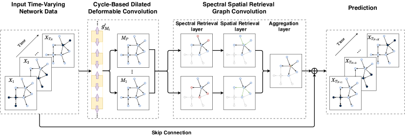
Figure 1: The framework of TSSRGCN. Cycle-Based Dilated Deformable Convolution block with kernel $g^{\prime}_{M_{i}}$ is firstly applied to capture $P$ temporal patterns with dilated rate $M_{i},i\in\{1,\ldots,P\}$. Stacked Spectral Spatial Retrieval Graph Convolution blocks model nodes and edges by extracting the locality and globality of the entire traffic network. Skip connection is utilized to concatenate input and embedding before the last fully-connected layer. The model is able to generate accurate traffic flow prediction from short term to long term.

II Preliminaries

Denote the traffic network as a directed weighted graph $G=(V,E,W^{0},W^{1})$ in this paper. Here, $V$ is the set of nodes with size $N=|V|$ and $E$ is the set of edges representing the road segments between sensors. $W^{0}\in\{0,1\}^{N\times N}$ and $W^{1}\in\mathbb{R}^{N\times N}$ are the general and weighted adjacency matrices respectively constructed based on the graph.

Sensors periodically measure and record traffic status indicators such as flows, occupancy, and speed. Let $T_{sp}$ denote the measuring frequency and $F$ denote the number of the recorded indicators. Given a time interval $[T_{begin},T_{end}]$, the traces of indicators recorded by $N$ sensors can be represented by $X\in\mathbb{R}^{N\times F\times T_{N}}$. $T_{N}=(T_{end}-T_{begin})/T_{sp}$ stands for the number of timesteps in the given interval.

The traffic flow forecasting task on the network aims to provide accurate predictions of the future flow, which can be formulated as: Given an traffic network $G=(V,E,W^{0},W^{1})$ and historical data $X=(X_{1},\ldots,X_{T_{N}})$ where $X_{T_{i}}\in\mathbb{R}^{N\times F}$ is data at timestep $T_{i}$, we are expected to learn a function $\Psi$ for prediction of traffic flow series $\hat{Y}=\Psi(X)=(\hat{Y}_{T_{N+1}},\ldots,\hat{Y}_{T_{N+K}})$ for all nodes in the next $K$ time steps after $T_{N}$, i.e.,:

$$\Psi^{*}=\arg\min_{\Psi}||\Psi(X)-Y||^{2},$$ (1)

Here $Y_{T_{i}}\in\mathbb{R}^{N}$ is the ground-truth flow at $T_{i}$ and $Y=(Y_{T_{N+1}},\ldots,Y_{T_{N+K}})$ is the time series to be forecasted.

III Temporal Spectral Spatial Retrieval Graph Convolutional Network

In this paper, we propose Temporal Spectral Spatial Retrieval Graph Convolution Network (TSSRGCN) for accurate traffic flow forecasting. The overall architecture of the proposed TSSRGCN is illustrated in Fig. 1. TSSRGCN consists of a cycle-based dilated deformable convolution block (CBDDC-block), stacked spectral spatial retrieval graph convolutional block (SSRGC-block) and a fully-connected layer for the final prediction. Skip connection [5] is applied to fuse the high-order knowledge learned from the stacked SSRGC-blocks and the low-order input features. The detailed design of TSSRGCN will be explained in this section.

III-A Cycle-Based Dilated Deformable Convolution Block

Cycle-Based Dilated Convolution. Dilated convolution is proposed by [6] in computer vision to exponentially expand the receptive field without loss of resolution. [7] adopts this in convolution block to learn temporal features of nodes. Different from the vanilla convolution, kernels of dilated convolution are sparse as the dilated rate is usually set to a power of two, i.e. $dr=2^{i},i\in\mathbb{N}^{+}$, with $dr$-1 pixels skipped.

Considering a series of traffic data collected in $T_{N}$ days and the dilated rate is $dr=2^{2}$, then it will extract information from data at day $1,5,\ldots,T_{4\times\lceil T_{N}/4\rceil-3}$, which maybe Monday, Friday, Next Tuesday, etc. The selected days does not form a regular traffic period, meaning the convolution receives a meaningless input series and thereby fails to retrieve knowledge of traffic patterns.

Intuitively, the traffic data may present three temporal evolution patterns [3]: daily/recent/weekly. The daily pattern implies that the temporal trend in every two adjacent days may be very similar, while Recent traffic status has a strong impact on current timestep for it is likely to continue the trend of previous timestep. The weekly pattern has two effects: the same moment in different weeks show a similar basic pattern, named discrete weekly periodicity; the traffic status continuously evolves from last week to this week due to various factors, named the continuous weekly trend. Existing research only focuses on weekly periodicity while ignores weekly trends, losing rich evolution information.

To incorporate the above temporal patterns, we propose a cycle-based dilated convolution block. The dilated rate is restricted to be chosen from a pre-define dilated rate set $\tau$. The daily pattern and two weekly evolution effects can be described in $\tau$ depending on the data sampling frequency $T_{sp}$. Note that more periods like monthly and seasonal one can be further defined with more data and computing resources. Given a period length (i.e., dilated rate) $M_{i}\in\tau$, the corresponding cycle-based dilated convolution on input $x_{s}(t)\in X_{t}$ of node $s$ at time step $t$ is depicted as

$$(g_{M_{i}}\star_{\tau}x_{s})(t)=\sum^{K_{S}(M_{i})-1}_{p=0}g_{M_{i}}(p)x_{s}(t-M_{i}\times p)$$ (2)

where $g_{M_{i}}\in\mathbb{R}^{K_{S}(M_{i})}$ is a dilated convolution kernel containing $K_{S}(M_{i})$ elements. The element of $g_{M_{i}}$ is indexed by $p$. $\star_{\tau}$ denotes the cycle-based dilated convolution over $\tau$.

Cycle-Based Dilated Deformable Convolution. The temporal dynamics could have some perturbation between two periods [8]; thus, fixed periods in $\tau$ ignore the period shifting, leading to biased learning. We adapt the deformable convolution [9] to tackle this problem. By adding learnable position shiftings to the kernels, convolution operation could adaptively represent various temporal patterns and be flexible to capture the variation of periods. The Cycle-Based Dilated Deformable Convolution block modifies Eqn. (2) by:

$$(g^{\prime}_{M_{i}}\star_{\tau}x_{s})(t)=\sum^{K_{S}(M_{i})-1}_{p=0}g^{\prime}_{M_{i}}(p)x_{s}(t-M_{i}\times p+\Delta p)$$ (3)

with $g^{\prime}_{M_{i}}\in\mathbb{R}^{K_{S}(M_{i})}$ as dilated deformable convolution kernel. $\Delta p$ is the position shifting for $p$-th kernel element.

In practice, we apply $P$ dilated deformable convolution layers to ensures that TSSRGCN would depict the temporal aspects of traffic networks over dynamic evolution patterns. The outputs of all layers $\mathcal{P}_{i},i\in\{1,\ldots,P\}$ will be concatenated and fed to a linear layer with learnable parameter $\Omega\in\mathbb{R}^{P\times F\times F_{T}}$ for feature fusion as the temporal representation for each node. The temporal representation is then taken as the input to the next block, denoted as $H_{0}=[\mathcal{P}_{1},...,\mathcal{P}_{P}]\Omega$, where $[,]$ is a concatenate operation and $F_{T}$ denotes the dimention of the temporal representation. In this case, the temporal aspect of traffic patterns is retrieved by the CBDDC layers with various dilated rates (i.e. CBDDC-block).

III-B Spectral Spatial Retrieval Graph Convolutional Block

TSSRGCN employs the Spatial Spectral Retrieval Graph Convolutional block (SSRGC-block) to investigate the sensors data and features of road segments on traffic network. A SSRGC-block is composed of a spectral retrieval layer, a spatial retrieval layer and an aggregation layer. Specifically, the spectral retrieval layer is applied to aggregate information from upstream and downstream nodes based on spectral methods, respectively. The node embedding learned by the spectral retrieval layer will be used to generate edge representations through the spatial retrieval layer with edge information from the weighted adjacency matrix. An aggregation operation finally aggregates edge representations to the connected nodes to retrieve the critical evidence for the forecasting. In practice, we stack $\lambda$ blocks in TSSRGCN for consideration of efficiency and accuracy.

Spectral Retrieval Layer. Spectral-based GCN utilizes adjacency matrix $W^{0}$ to aggregate information from neighborhood nodes. For example, [10] proposes a diffusion convolution layer with the motivation that spatial structure in traffic is non-Euclidean and directional; thus, upstream and downstream nodes can have different influence on current nodes. We adapt the diffusion convolution layer to spread the messages over two directions. Let $A_{d}=D_{d}^{-1}W^{0}$ denote the transition matrix, which measures the probability that information of current node transfers to its downstream neighbor, where $D_{d}=\text{diag}(W^{0}\textbf{1})$ is out-degree matrix. Similarly, $A_{u}=D_{u}^{-1}{W^{0}}^{\mathsf{T}}$ could be used to gather information from upstream neighborhood with $D_{u}=\text{diag}({W^{0}}^{\mathsf{T}}\textbf{1})$ as in-degree matrix. The $l$-th ($l\in\{1,\ldots,\lambda\}$) spectral retrieval layers can be formulated as

$$\begin{split}&V^{l}_{u}=\sigma(\theta^{l}_{u}(A_{u}+I)H_{u}^{l}),\\ &V^{l}_{d}=\sigma(\theta^{l}_{d}(A_{d}+I)H_{d}^{l}),\end{split}$$ (4)

where $V^{l}_{u},V^{l}_{d}\in\mathbb{R}^{N\times F_{T}}$ is the upstream and downstream node embedding after $l$-th spectral retrieval layer. $H^{l}_{u},H^{l}_{d}$ denotes the output from $(l-1)$-th SSRGC-block. In particular, $H^{0}_{u}=H^{0}_{d}=H_{0}$ is the temporal representations from the CBDDC-block. $\theta^{l}_{u},\theta^{l}_{d}\in\mathbb{R}$ is learnable parameters of spectral retrieval layers. $\sigma(\cdot)$ is the sigmoid activation.

Spatial Retrieval Layer. Apart from nodes of the traffic network, road segments of traffic network also play essential roles in revealing traffic system status. Features of road segments such as length, geographical location, and the number of lanes, may greatly influence the adjacent nodes. However, recent studies [11, 3, 7, 12] mainly focus on extracting node embedding, instead of modeling the significance of the edges. Beyond these, locality and globality can also be simultaneously modeled when considering edges and its adjacent nodes. Globality represents the absolute flow of nodes since high flow indicates congestion, while low flow means the road segments are clear. Locality reveals the transition volume of flows between the upstream and the downstream nodes in the near future. As the traffic network is highly dynamic, the spatial-correlation of the traffic network should be well captured through edge representations.

Given an edge $s_{1}\to s_{2}$, we model the locality and globality by edge representation following spatial-based GCN. Specifically, the upstream edge representation $e_{u,s_{1}s_{2}}^{l}$ from node $s_{1}$ to node $s_{2}$ of $l$-th layer can be obtained by

$$e_{u,s_{1}s_{2}}^{l}=f_{\Theta^{l}_{u}}(V_{u,s_{1}}^{l},V_{u,s_{2}}^{l}-V_{u,s_{1}}^{l},W^{1}_{s_{1}s_{2}})$$ (5)

where $f_{\Theta^{l}_{u}}(\cdot)$ is spatial retrieval layer with learnable parameter $\Theta^{l}_{u}$. The spatial retrieval layer is expected to fuse the features in global aspects as well as local aspects, where $V_{u,s_{1}}^{l}$ is utilized to stand for the status of node $s_{1}$ from perspective of the global traffic network while $V_{u,s_{2}}^{l}-V_{u,s_{1}}^{l}$ represents the relative value of locality on edge $s_{1}\to s_{2}$. $W^{1}_{s_{1}s_{2}}$ denotes static edge features between $s_{1}$ and $s_{2}$. With this design, globality, locality and the static edge information are incorporated via the spatial retrieval function $f_{\Theta}(\cdot)$.

Similarly, the downstream edge representation $e_{d,s_{2}s_{1}}^{l}$ from $s_{2}$ to $s_{1}$ of $l$-th layer would be depected by:

$$e_{d,s_{2}s_{1}}^{l}=f_{\Theta^{l}_{d}}(V_{d,s_{2}}^{l},V_{d,s_{1}}^{l}-V_{d,s_{2}}^{l},W^{1}_{s_{2}s_{1}}).$$ (6)

The edge representations are learned from both explicit and implicit features of the traffic network (RQ3). As each sensor is usually connected to a small number of roads in real-world traffic network, the number of learned edge representation is in the scale of $\mathcal{O}(N)$. To avoid further increase the complexity, we employ concatenation without parameters for both function $f_{\Theta^{l}_{d}}(\cdot)$ and $f_{\Theta^{l}_{u}}(\cdot)$.

Aggregation Layer. Inspired by [13] which chooses the k-nearest points of current node of the point cloud in 3D space and aggregates their information, we utilize an aggregation layer to amalgamate the edge representation. Intuitively, the most significant impact on node $s_{1}$ may come from its neighbor nodes with the shortest distance. In view of this rule, the aggregation layer to learn node embedding $H^{l+1}_{u,s_{1}}$ from upstream direction at $l+1$th block is designed as

$$H^{l+1}_{u,s_{1}}=\bigcup_{s_{2}\in N_{d,k}(s_{1})}\psi^{l}_{d,s_{2}}e_{u,s_{1}s_{2}}^{l}+\bigcup_{s_{3}\in N_{u,k}(s_{1})}\psi^{l}_{u,s_{3}}e_{u,s_{3}s_{1}}^{l}$$ (7)

where $\bigcup$ is an aggregation operation (e.g, summation or mean). $N_{u,k}(i)$ and $N_{d,k}(i)$ represent a set of $k$-nearest neighborhood node of node $i$ from upstream and donwstream seperately. $k$ can be set as the average degree of the traffic network. $\psi^{l}_{d,s}$ and $\psi^{l}_{u,s}$ are learnable parameters indicating the significance of nodes during the aggregation, and they are shared for all nodes in the traffic network for efficiency concern. The node embedding $H^{l+1}_{d,s_{1}}$ from downstream direction can be defined in a similar way.

Finally, the outputs of each SSRGC-block are concatenated to capture both high-order features and low-order features. Thus, globality and locality are both considered by TSSRGCN over the node embedding and edge representations (RQ2). Specifically, we use a $1\times 1$ convolution layer to reduce the dimension to $F_{S}$.

III-C Forecasting Layer

We adopt skip connection [5] to concatenate input $X$ with output of the aggregation layer $H$ as input to the forecasting layer. To improve the efficiency, we directly use a fully connected layer to generate predicted value $\hat{Y}$ on each node at all $K$ time steps. TSSRGCN is set to minimize the L2-loss between the predicted value $\hat{Y}$ and ground-true value $Y$, i.e., $\mathcal{L}(\hat{Y},Y)=\|\hat{Y}-Y\|^{2}$.

IV Experiments

In this section, we conduct experiments over real-world traffic datasets to examine the performance of TSSRGCN. We decomposite the RQs and design experiments to answer the following questions: Q1: How does our model perform compared to other state-of-the-art traffic flow forecasting models? Q2: Can our model capture the short-term and long-term temporal evolution patterns?

IV-A Experiment Setup

Datasets. We evaluate our model on two real-world traffic datasets PEMSD3 and PEMSD7. These datasets are collected by California Transportation Agencies (CalTrans) Performance Measurement System (PeMS) [14] by every 30 seconds, where the traffic flow around the sensors are reported (i.e., $F=1$). The data are aggregated into every 5-minutes interval. The datasets also contain the metadata of the sensor network from which we can build the graph $G$.

PeMSD3 contains data with 358 sensors in North Central Area from Sep. 1st to Nov. 30th in 2018. PeMSD7 contains data with 1047 sensors in San Francisco Bay Area from Jul. 1st to Sep. 30th in 2019.

TABLE I: Performance comparison of TSSRCNN and other baseline methods on PEMSD3.

PEMSD3	15 min			30 min			60 min
Model	MAE	RMSE	MAPE($\%$)	MAE	RMSE	MAPE($\%$)	MAE	RMSE	MAPE($\%$)
SVR	18.28	29.98	24.44	21.00	33.66	26.10	24.33	38.87	29.46
LSTM	17.12	28.34	22.57	18.92	31.12	24.40	22.28	36.06	29.09
DCRNN	14.81	24.43	14.22	16.80	27.64	15.85	20.39	32.93	19.13
STGCN	14.78	27.15	21.45	16.83	29.79	24.32	20.59	34.93	28.19
ASTGCN	16.14	27.45	16.48	17.41	29.90	17.68	19.16	33.32	19.49
Graph WaveNet	14.61	24.89	15.00	16.50	28.11	15.68	20.12	33.38	18.32
STSGCN	14.82	23.92	14.74	15.81	25.64	15.52	17.61	28.69	16.95
TSSRGCN	13.49	20.40	13.99	13.81	21.10	14.15	14.22	21.87	14.52

TABLE II: Performance comparison of TSSRGCN and other baseline methods on PEMSD7

PEMSD7	15 min			30 min			60 min
Model	MAE	RMSE	MAPE($\%$)	MAE	RMSE	MAPE($\%$)	MAE	RMSE	MAPE($\%$)
SVR	21.94	35.13	12.64	25.33	39.90	13.94	31.10	48.42	16.92
LSTM	20.98	34.36	12.10	24.27	38.62	12.40	29.49	46.55	16.06
DCRNN	20.00	32.71	10.17	22.70	36.90	11.53	27.59	44.06	14.39
STGCN	20.25	32.12	10.23	23.39	36.42	11.60	29.32	44.61	14.28
ASTGCN	19.61	31.58	10.67	20.78	33.61	11.25	22.34	36.37	12.14
Graph WaveNet	20.36	33.18	10.67	23.28	37.75	12.36	28.56	45.54	15.09
STSGCN	20.03	31.79	10.54	21.33	33.88	11.14	23.57	37.43	12.25
TSSRGCN	17.95	28.20	10.86	18.59	29.31	11.03	19.38	30.64	11.64

Preprocessing. The sampling frequency $T_{sp}$ is 5 minutes for two datasets, and there are 288 timesteps in one day. The missing data are calculated by linear interpolation. Besides, the input data are transformed by zero-mean normalization.

$W^{0}$ is adjacency matrix revealing real edges between nodes on the graph. $W^{1}$ is distance-base adjacency matrix which is defined as $W^{1}_{s_{i}s_{j}}=\exp\left(-\frac{d_{s_{i}s_{j}}^{2}}{\sigma_{d}^{2}}\right)$ if $s_{i}\neq s_{j}$ and $\exp\left(-\frac{d_{s_{i}s_{j}}^{2}}{\sigma_{d}^{2}}\right)\geq\epsilon$. Here $d_{s_{i}s_{j}}$ denotes the distance between sensors $s_{i}$ and $s_{j}$. $\sigma_{d}$ is the standard deviation of distance and $\epsilon$ is 0.5 to control the sparsity of $W^{1}$ according to [11].

Settings. We implement TSSRGCN by PyTorch and select mean operation in the aggregation layer. Adam [15] is leveraged to update the parameters during training for a stable and fast convergence. The datasets are split into training/validation/test sets with ratio 6:2:2 in the time dimension. Our task is to forecast traffic flow in the next hour as $K=12$. We use the last hour data before the predicted time as the recent data, and the same hour of the last seven days to extract daily pattern and weekly pattern (daily pattern only requires the last three days’ data). In this case, $\tau=\{1,12,84\}$ and we fix $P=3$ to capture the recent/daily/weekly patterns and the corresponding period shiftings. There are $T_{N}=96$ time steps in total. The batch size is 64 for PEMSD3 and 16 for PEMSD7 as the latter is about three times larger than the former. $F_{T},F_{S}$ and $k$ is 64, 64 and 3 for both dataset. We set 1e-2 as the learning rate for PEMSD3 and 3e-3 for PEMSD7. $\lambda$ is 4 for PEMSD3 and 5 for PEMSD7.

Baseline Methods. We compare our model with the following baselines and we use the optimal hyperparameters of these methods mentioned in the corresponding paper: SVR [16], LSTM [17], DCRNN [10], STGCN [11], ASTGCN [3], Graph WaveNet [7], STSGCN [12].

Evaluation Metric. To evaluate the performance of different models, we adopt Mean Absolute Errors (MAE), Root Mean Squared Errors (RMSE) and Mean Absolute Percentage Errors (MAPE) as our metric.

IV-B Experimental Results (Q1 and Q2)

We discuss the performace of TSSRGCN and other baselines, and compare the results over different time windows.

Overall Performance (Q1). We compare TSSRGCN with seven models on PeMSD3 and PeMSD7. Tab. I and Tab. II show the performance on the forecasting task at different time granularity (i.e., 15-, 30-, and 60-mins in the future). We can conclude that: (1) Deep learning methods, especially models based on GCNs, perform better than traditional ones. Due to the complex spatial-temporal correlation of traffic networks, traditional methods fail to capture the latent features of all nodes at all time steps. LSTM can extract some temporal information from the traffic data, which helps improve the prediction compared with SVR. GCNs based models are compelling on mining graph structure data when solving our task, outperforming general deep learning model in many metrics. (2) TSSRGCN performs well on both datasets, verifying the robustness of our model to various traffic patterns and different scales of nodes in the graph.

Performance on Different Time Windows (Q2). To show the ability to extract short and long term temporal information, we conduct TSSRGCN on various time windows. We can find that: (1) TSSRGCN achieves state-of-the-art results in medium and long term (30 and 60 mins) as the long-period information is captured in the CBDDC block, indicating that periodic patterns contribute to extract temporal correlation. (2) TSSRGCN presents competitive performance to the best result on the prediction in the near future (i.e., 15-min), which can be attributed to the combination of both locality and globality. (3) Models mining various temporal patterns can perform well both in the short and long term (i.e., ASTGCN and TSSRGCN).

V Conclusion

In this paper, we propose TSSRGCN for traffic flow forecasting. Motivated by the fact that there exist different temporal traffic patterns with period shifting, TSSRGCN employs the cycle-based dilated convolution blocks to incorporate the temporal traffic patterns from both short-term and long-term aspects. Meanwhile, GCNs for learning node embeddings and edge representations are stacked to retrieve spectral and spatial features from traffic network. Experiments on two real-world datasets show that our model performs well on different metrics compared to state-of-the-art methods, indicating robustness of the proposed method on various temporal patterns and the practicability to help administrator regulate the traffic in the real world.

References

- [1] B. M. Williams and L. A. Hoel, “Modeling and forecasting vehicular traffic flow as a seasonal arima process: Theoretical basis and empirical results,” Journal of transportation engineering, vol. 129, no. 6, pp. 664–672, 2003.
- [2] M. Castro-Neto, Y.-S. Jeong, M.-K. Jeong, and L. D. Han, “Online-svr for short-term traffic flow prediction under typical and atypical traffic conditions,” Expert systems with applications, vol. 36, no. 3, pp. 6164–6173, 2009.
- [3] S. Guo, Y. Lin, N. Feng, C. Song, and H. Wan, “Attention based spatial-temporal graph convolutional networks for traffic flow forecasting,” in Proceedings of the AAAI Conference on Artificial Intelligence, vol. 33, 2019, pp. 922–929.
- [4] M. Defferrard, X. Bresson, and P. Vandergheynst, “Convolutional neural networks on graphs with fast localized spectral filtering,” in Advances in neural information processing systems, 2016, pp. 3844–3852.
- [5] K. He, X. Zhang, S. Ren, and J. Sun, “Deep residual learning for image recognition,” in Proceedings of the IEEE conference on computer vision and pattern recognition, 2016, pp. 770–778.
- [6] F. Yu and V. Koltun, “Multi-scale context aggregation by dilated convolutions,” arXiv preprint arXiv:1511.07122, 2015.
- [7] Z. Wu, S. Pan, G. Long, J. Jiang, and C. Zhang, “Graph wavenet for deep spatial-temporal graph modeling,” arXiv preprint arXiv:1906.00121, 2019.
- [8] H. Yao, X. Tang, H. Wei, G. Zheng, and Z. Li, “Revisiting spatial-temporal similarity: A deep learning framework for traffic prediction,” in Proceedings of the AAAI Conference on Artificial Intelligence, vol. 33, 2019, pp. 5668–5675.
- [9] J. Dai, H. Qi, Y. Xiong, Y. Li, G. Zhang, H. Hu, and Y. Wei, “Deformable convolutional networks,” in Proceedings of the IEEE international conference on computer vision, 2017, pp. 764–773.
- [10] Y. Li, R. Yu, C. Shahabi, and Y. Liu, “Diffusion convolutional recurrent neural network: Data-driven traffic forecasting,” arXiv preprint arXiv:1707.01926, 2017.
- [11] B. Yu, H. Yin, and Z. Zhu, “Spatio-temporal graph convolutional networks: A deep learning framework for traffic forecasting,” arXiv preprint arXiv:1709.04875, 2017.
- [12] C. Song, Y. Lin, S. Guo, and H. Wan, “Spatial-temporal sychronous graph convolutional networks: A new framework for spatial-temporal network data forecasting,” 2020.
- [13] Y. Wang, Y. Sun, Z. Liu, S. E. Sarma, M. M. Bronstein, and J. M. Solomon, “Dynamic graph cnn for learning on point clouds,” ACM Transactions on Graphics (TOG), vol. 38, no. 5, pp. 1–12, 2019.
- [14] C. Chen, K. Petty, A. Skabardonis, P. Varaiya, and Z. Jia, “Freeway performance measurement system: mining loop detector data,” Transportation Research Record, vol. 1748, no. 1, pp. 96–102, 2001.
- [15] D. P. Kingma and J. Ba, “Adam: A method for stochastic optimization,” arXiv preprint arXiv:1412.6980, 2014.
- [16] H. Drucker, C. J. Burges, L. Kaufman, A. J. Smola, and V. Vapnik, “Support vector regression machines,” in Advances in neural information processing systems, 1997, pp. 155–161.
- [17] S. Hochreiter and J. Schmidhuber, “Lstm can solve hard long time lag problems,” in Advances in neural information processing systems, 1997, pp. 473–479.