Cooperative states and shift in resonant scattering of an atomic ensemble

Abstract

We investigate the spectral shift in collective forward scattering for a cold dense atomic cloud. The shift, sometimes called collective Lamb shift, results from resonant dipole-dipole interaction mediated by real and virtual photon exchange, forming many-body states displaying various super- and subradiant spectral behavior. The scattering spectrum reflects the overall radiative behavior from these states. However, it also averages out the radiative details associated with a single collective state, causing ambiguity in explaining the origin of the spectral shift and raising controversy on its scaling property. We employ a Monte-Carlo simulation to study how the collective states are occupied and contribute to emission. We thus distinguish two kinds of collective shift that follow different scaling laws. One results from dominant occupation of the near-resonant collective states. This shift is usually small and insensitive to the density or the number of participating atoms. The other comes from large spatial correlation of dipoles, associated with the states of higher degree of emission. This corresponds to larger collective shift that is approximately linearly dependent on the optical depth. Our analysis provides not only a novel perspective for the spectral features in collective scattering, but also a possible resolution to the controversy on the scaling property that has been reported elsewhere because of different origins.

Light-ensemble interaction has been an important topic drawing continuing attention for recent years thanks to its fundamental interest in quantum many-body physics and practical applications in various areas, such as atomic clocks and metrology (Takamoto et al., 2005; Ludlow et al., 2015), sensing and precision measurement (Kitching et al., 2011), quantum simulation (Bloch et al., 2012), quantum interface, memory, and network (Duan et al., 2001; Lukin, 2003; Kimble, 2008; Kómór et al., 2014). In various proposals, schemes based on atomic ensembles are expected to have enhanced coupling strength for more efficient manipulation by increasing the number and/or density of atoms. As the system becomes sufficiently dense, on the other hand, cooperative effects due to atoms’ dipole-dipole interaction start to emerge, including super- and subradiance, directional emission, frequency shift, and distortion of line shape (Guerin et al., 2017). These effects may, for instance, cause unwanted decoherence in quantum control and degrade the precision of optical atomic clocks (Chang et al., 2004). Thus, how to understand the cooperativity in atomic ensembles not only provides insightful perspectives for many-body physics in the presence of nontrivial competing interactions, but also helps develop quantum optical devices and applications more accurately.

One intriguing cooperative phenomenon is the emergence of the collective Lamb shift, the many-body version of the ordinary Lamb shift. The ordinary Lamb shift accounts for the vacuum fluctuations that perturb the electron’s orbital in an atom and introduce an energy shift (Welton, 1948). Understanding of this shift has opened a new subject now known as quantum electrodynamics. To correctly calculate the shift, contributions of all transition processes including virtual ones need to be properly dealt with. Similar consideration applies to many-body cases, where both the real and virtual processes of photon exchange mediate the dipole-dipole interaction, resulting in cooperative decay and energy shift of the collective states. Recently, such phenomena have attracted extensive attention, and have been discussed in various contexts including atomic clouds (Jennewein et al., 2016; Araújo et al., 2016; Roof et al., 2016; Bromley et al., 2016), nano-layer gases (Keaveney et al., 2012; Peyrot et al., 2018), ensembles of nuclei (Röhlsberger et al., 2010), trapped ions (Meir et al., 2014), and artificial atoms (van Loo et al., 2013; Wen et al., 2019; Lin et al., 2019). Another perspective views this shift as coupling between collective states, leading to Rabi-like excitation transfer among a few atoms (Barredo et al., 2015; Browaeys et al., 2016).

A commonly-used technique to detect the collective shift is through scattering experiments, where one measures the emission spectrum while sweeping the probe frequency, and extracts the shift of the spectral peak. Though it is valid to consider only the lowest excited manifold for weak probing, as in many experiments, there are $N$ such singly-excited states with $N$ the number of atoms in the ensemble, and these states are shifted differently owing to competing dipole-dipole interaction. Unfortunately, the scattering spectrum only reflects the overall effect of superposed contributions from individual collective states. Some unrevealed spin orders relevant to the spectrum might be averaged out. Further, there have been controversies regarding the scaling nature of the collective shift in different geometries such as slabs and ellipsoids. Recent experiments have reported large collective shift in elongated atomic samples (Roof et al., 2016; Jennewein et al., 2016) but negligible shift in pancake-like clouds (Corman et al., 2017). Changing the anisotropy also introduces unusual shift scaling (Bromley et al., 2016). For some specific geometries and densities, the lineshape becomes asymmetric and even displays two peaks in the profile, making the determination of the shift ambiguous.

To better understand the underlying mechanisms, in this manuscript we look into the roles of the many-body states by choosing an appropriate orthogonal basis. We adopt a Monte-Carlo simulation by randomly distributing atoms of controlled density within a given geometry, and use the standard non-Hermitian Schrodinger equation approach in the weak-field (single-excitation) limit. Note that this is a special case where the mathematical structure is consistent with the classical dipole analysis. For each run, the randomly picked spatial arrangement of atoms is called a configuration in this manuscript. The calculated outcomes display huge fluctuations from run to run, implying the sensitivity of the system to the actual parameters. The robustness of the results lies in the ensemble averaged profiles as we try many configurations. Let’s first look at one of the most illustrative examples corresponding to a uniform dense cylindrical sample of radius comparable to a transition wavelength and length over a few wavelengths. Fig. 1 shows the corresponding scattering spectrum, excitation distribution, and emission capability, defined to characterize the spectral contribution of a state (see following discussions). We can observe “three peaks” in the spectrum by sweeping the probe detuning: the strongest left peak, the small tip in the center, and the smooth hump on the right. Similar spectral profiles have also been discussed in (Sokolov et al., 2009, 2011). We find that the three peaks have different origins by taking into consideration the roles played by the participating collective states. Such diagnosis applies to general cases but the significance of the three types of contribution may vary in different geometries and parameters. For instance, the smooth hump on the blue side only emerges in cases close to uniform distribution of atoms, and easily smears out in Gaussian samples. The large shift on the left is more pronounced in elongated systems, and gradually merges to the center peak as the anisotropy reduces. Note that the central peak is also shifted, as shown in the inset of Fig. 1(a). Most of the collective shift measurements refer to either the left or the central peak (the right hump is usually not very contrastive), which yields very different scaling nature.

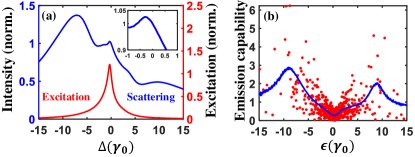
Figure 1: (a) Forward scattering (blue) and total excitation (red) spectrum (ensemble averaged). Inset: zoomed plot near the central tip of the scattering spectrum. The three peaks are located at $\Delta=-7.3\gamma_{0}$, $-0.2\gamma_{0}$, and $+9.6\gamma_{0}$. (b) Emission capability versus the eigenenergy $\epsilon$ (compatible to the state shift) of the corresponding collective state. The scattered dots are from a single configuration and the blue curve is from ensemble average. The system used here is a cylindrical atomic ensemble of radius $R=2\pi c/\omega_{0}$ and length $L=3R$. The laser incident direction is along the axis of the cylinder. The ensemble average is done by considering $>5000$ random configurations of atoms uniformly distributed inside the cylinder with $\rho/k^{3}=0.3$, where $\rho$ is the number density. (The scattering spectrum and excitation curves are normalized by the values at $\Delta=0$. The emission capability is in arbitrary units.)

We consider an ensemble of $N$ two-level atoms randomly distributed in a localized region of certain geometry with $\boldsymbol{r}_{i}$ denoting the location of the $i$th atom assumed to be fixed in space. To probe the spectrum scattered by the singly-excited collective states and the associated Lamb shift, these atoms are driven weakly by a laser beam propagating along the $+z$ direction, where the detuning $\Delta\equiv\omega-\omega_{0}\ll\omega_{0}$, wavevector $\bm{k}\equiv\omega\hat{z}/c\approx\omega_{0}\hat{z}/c$, Rabi frequency $\Omega\ll\gamma_{0}$, with $\omega_{0}$ ($\omega$) the atomic (laser) frequency and $\gamma_{0}$ the spontaneous emission rate, and $c$ the speed of light. In the low-excitation limit, a quantum state can be of the form $|\psi\rangle\approx|g_{1}\cdots g_{N}\rangle+\sum_{i}b_{i}|g_{1}\cdots e_{i}\cdots g_{N}\rangle$ with $|b_{i}|\ll 1$, which satisfies $i\dot{\bm{B}}(t)=\mathbf{M}\bm{B}+\Omega\bm{D}$ (Zhu et al., 2016), where $\bm{B}=\left[b_{1},\ldots,b_{i},\ldots,b_{N}\right]^{\intercal},$ $\bm{D}=\left[e^{i\bm{k}\cdot\bm{r}_{1}},\ldots,e^{i\bm{k}\cdot\bm{r}_{i}},\ldots,e^{i\bm{k}\cdot\bm{r}_{N}}\right]^{\intercal}$, and

$$\bm{\mathbf{M}}=\begin{bmatrix}-\Delta-\frac{i\gamma_{0}}{2}&V_{12}&\cdots&V_{1N}\\ V_{21}&-\Delta-\frac{i\gamma_{0}}{2}&\cdots&\vdots\\ \vdots&\vdots&\ddots&\vdots\\ V_{N1}&\cdots&\cdots&-\Delta-\frac{i\gamma_{0}}{2}\end{bmatrix}.$$ (1)

The dipole-dipole interaction is given by

$$V_{ij}=\frac{3\gamma_{0}}{4}\Big{[}-\left(1-\cos^{2}\theta_{ij}\right)\frac{e^{ikr_{ij}}}{kr_{ij}}+\\ \left(1-3\cos^{2}\theta_{ij}\right)\left(\frac{-ie^{ikr_{ij}}}{(kr_{ij})^{2}}+\frac{e^{ikr_{ij}}}{(kr_{ij})^{3}}\right)\Big{]},$$ (2)

depending on the separation $r_{ij}=|\bm{r}_{j}-\bm{r}_{i}|$ between two atoms $i$ and $j$, and the angle $\theta_{ij}$ between the distance vector $\bm{r}_{j}-\bm{r}_{i}$ and the dipole orientation assumed to be the $x$ direction for linear polarized driving field. The dipole-dipole interaction couples the $N$ singly excited states, causing various degrees of shift depending on the configuration of distribution of the atoms. When $N$ is large, it is however unrealistic and meaningless to measure the shift of each collective state. Nevertheless, the scattering spectrum still catch the overall contributions, and can help identify the emergence and order of magnitude of the collective Lamb shift. But we still need to look into what are actually probed for further diagnosis.

By solving $\bm{B}=-\Omega\mathbf{M}^{-1}\bm{D}$, we obtain the steady-state solution $b_{i}$, which determines the intensity of the forward scattering by $I\propto\left|\sum_{i}b_{i}e^{-i\bm{k}\cdot\bm{r}_{i}}\right|^{2}=\sum_{i}\left|b_{i}\right|^{2}+\sum_{i\neq j}b_{i}b_{j}^{*}e^{-i\bm{k}\cdot(\bm{r}_{i}-\bm{r}_{j})}$. We identify two parts: the incoherent scattering term $\sum_{i}\left|b_{i}\right|^{2}$ and the coherent one $\sum_{i\neq j}b_{i}b_{j}^{*}e^{-i\bm{k}\cdot(\bm{r}_{i}-\bm{r}_{j})}$. The former exactly corresponds to the total excitation of individual atoms for a given probe detuning. The latter accounts for the spin-spin correlation modulated by the spatial phases. The resultant spectral profile of emission fluctuates drastically for a given spatial configuration of atoms. We thus take the ensemble average over many configurations, and generate a convergent coarse-grained profile, as shown in Fig. 1.

To understand the spectrum, it is natural to relate the radiative properties to the many-body states that are relevant. Note that the coupling matrix $\mathbf{M}$ is symmetric but complex. In some previous literature, it has been directly diagonalized to find the dynamics for the system (Li et al., 2013; Schilder et al., 2016; Guerin and Kaiser, 2017). The collective basis states thus found are however not orthogonal. Though the calculated dynamics is correct, it fails to associate the radiative behavior with specific states because they are seriously overlapped (Li et al., 2013). Here, by noting that $\mathbf{M}=-\Delta\mathbf{I}+\mathbf{M}_{R}+i\mathbf{M}_{I}$, where $\mathbf{I}$ is an $N\times N$ identity matrix, $\mathbf{M}_{R}$ and $\mathbf{M}_{I}$ are the real and imaginary parts of $\mathbf{M}$, respectively, we choose the orthogonal eigenbasis that diagonalizes only the real part $\mathbf{M}_{R}$ such that $\mathbf{M}_{R}^{D}=\mathbf{R}^{\intercal}\mathbf{M}_{R}\mathbf{R}$ with $\left[\mathbf{M}_{R}^{D}\right]_{ij}=\epsilon_{j}\delta_{ij}$. The eigenvalue $\epsilon_{j}$ is associated with an eigenvector $\bm{R}_{j}$ (the $j$th column of $\mathbf{R}$), and can be understood as the shift of the $j$th collective state $|\bm{R}_{j}\rangle=\sum_{s}\bm{\mathbf{R}}_{sj}|g_{1}\cdots e_{s}\cdots g_{N}\rangle$.

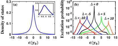
Figure 2: (a) Density of states (normalized by the area underneath). Inset: zoomed plot around the tip, which is red shifted by about $0.2\gamma_{0}$ to the single atom’s resonance. (b) Histogram of the excitation distribution (arbitrary unit) of at various detunings. (These curves are also ensemble averaged.)

Figure 2(a) shows the density of states as a function of a state’s shift $\epsilon$. The profile suggests that the majority of the collective states ($\sim 82.3\%$) have shift less than $5\gamma_{0}$. The density-of-state profile has a peak slightly shifted to the red side of the resonant one ($\epsilon=0$), which results in the shift of the central peak. We can now discuss the excitation $\left|p_{j}\right|^{2}$ of the state $|\bm{R}_{j}\rangle$ by applying a pumping laser of frequency $\omega=\omega_{0}+\Delta$. The steady-state solution $\bm{B}=\sum_{j}p_{j}\bm{R}_{j}$, and therefore $p_{j}=\left(\mathbf{R}^{-1}\bm{B}\right)_{j}$. We plot the excitation histogram of different shift for various detuning $\Delta$ in Fig. 2(b). As expected, the probe field excites only those states resonant to the laser frequency ($\Delta\approx\epsilon$) with a linewidth comparable to $\gamma_{0}$. The peak values of excitation also drops significantly for large $|\Delta|$ since the density of states is small of large $|\epsilon|$. We emphasize that the excitation behavior shown in Fig. 2(b) is only valid in this choice of orthogonal basis (from $\mathbf{M}_{R}$).

As we sweep the detuning, we might have expected that there would be a significant peak in the center of the spectrum, corresponding to the most probable excited states indicated by Fig. 2(a). In fact, this is not the case here. Those most-populated states only contribute to a small tip in the spectrum. By contrast, the most significant peak appears on the red side ($\Delta\approx-7.3\gamma_{0}$ in Fig. 1(a)). But the corresponding peak excitation is lower by two orders of magnitude than that of $\Delta=0$. This suggests that these states, though just a few of them, are much more radiative compared to the majority of the collective states. To quantify for the spectral contribution of a state, we define for the state $|\bm{R}_{j}\rangle$ the emission capability

$$\Pi_{j} =\left|\sum_{i}\bm{R}_{j}^{(i)}e^{-i\bm{k}\cdot\bm{r}_{i}}\right|,$$ (3)

where $\bm{R}_{j}^{(i)}$ is the $i$th element (corresponding to the $i$th atom) of the eigenvector $\bm{R}_{j}$. Since $I\propto\left|\sum_{i,j}p_{j}\bm{R}_{j}^{(i)}e^{-i\bm{k}\cdot\bm{r}_{i}}\right|^{2}$, if $\Pi_{j}$ is large (small), it can be expected that the state $|\bm{R}_{j}\rangle$ takes part significantly (insignificantly) in the scattering spectrum. It helps us to diagnose the behavior of each collective state and provides a novel perspective regarding super- and subradiance without explicitly taking into account the collective decay rates.

In Fig. 1(b), we plot the emission capability for a single configuration (red dots) and on average (blue line). We find that the emission capacity curve has two peaks around $\epsilon\approx-8.2\gamma_{0}$ and $\epsilon\approx+9.1\gamma_{0}$, implying that these states are highly capable of emission. The left peak does give rise to the most visible peak in the spectrum of Fig. 1(a). The right peak is also responsible for a small hump at the corresponding detuning of the spectral profile. This hump on the blue side is however less evident because the corresponding states are less populated. On the other hand, the states of small shift have low emission capability even though they are mostly populated. This “M-shaped” feature of emission capability is generally observed in all atomic configurations, even in various geometries and densities. But the actual spectral curves are still determined by considering overall the emission capability, density of states, excitation, and cross-term interference of the collective states in detail, which vary from sample to sample of different parameters.

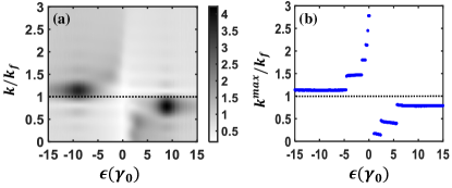
Figure 3: (a) Fourier spectrum of the spatial frequency versus eigenenergy with the color darkness (arbitrary unit) represents $F(\epsilon,k_{f})$. (b) Maximal spatial frequency extracted from (a).

Note that the probe detuning has nothing to do with the structure of the collective states $|\bm{R}_{j}\rangle$, which are determined solely by the interaction detail, $\mathbf{M}_{R}$. But the probe sets a detuning window that selects which collective states are pumped. Therefore, the scattered signal must reflect the spatial order of the picked states. The definition of emission capability Eq. (3) is a reminiscence of the Fourier transform of $\bm{R}_{j}$. We further define

$$\tilde{F}_{j}(k_{f})=\sum_{i}\bm{R}_{j}^{(i)}e^{-ik_{f}z_{i}},$$ (4)

which bares the information of components with “spatial frequencies” $k_{f}$ for a given state $|\bm{R}_{j}\rangle$. Here, we only focus on the spatial variation along the $+z$ propagation axis for forward scattering. We show the ensemble-averaged Fourier spectrum $F(\epsilon,k_{f})\equiv\left\langle\left|\tilde{F}_{j}(k_{f})\right|\right\rangle$ (averaged over $j$ of similar $\epsilon$) in Fig. 3(a). The dotted line refers to $k_{f}=k=2\pi/\lambda$, taken as a reference of spatial order in periods of $\lambda$. Further, the pattern of $F(\epsilon,k_{f})$ on both the red and blue sides appears to be stripe-like. For a given $\epsilon$, we identify the spatial frequency $k_{f}^{max}(\epsilon)$ that maximizes $F(\epsilon,k_{f})$, plotted in Fig. 3(b). We observe that the states who possess the most distinct spatial ordering (darkest spots in Fig. 3(a)) coincide with those of highest emission capability. This can be expected because the characteristic $k_{f}^{max}(\epsilon)$ of these states is closest to $k$, i.e., matching the spatial modulation of the incident light. This spatial ordering implies the cooperative nature of superradiance, and thus contributes significantly to the emission. By contrast, the states of small $|\epsilon|$ do not display a clear spatial order. This is due to random phase cancellation from averaging out a huge amount of such collective states. Note that the discreteness of $k_{f}^{max}$ is a reminiscence of the standing wave conditions, for which we find the spatial frequency gap $\Delta k_{f}^{max}\sim 2\pi/L$. But we do not have exactly $k_{f}^{max}=k$. This might be due to the size effect of a finite cylinder.

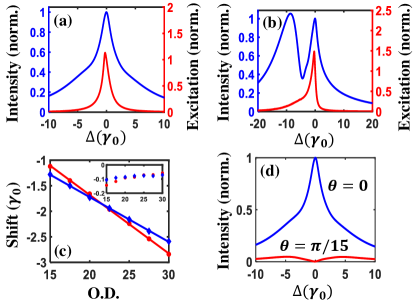
Figure 4: (a) Spherical Gaussian ensemble with $N=1000$ and $\sigma_{x,y,z}=\lambda_{0}$. (b) Cigar-shaped ensemble with $N=1000$, $\sigma_{x}=\sigma_{y}=0.5\lambda_{0}$ and $\sigma_{z}=4\lambda_{0}$. (c) Collective shift for varied OD. Red solid circles correspond to changing the system size by fixing the aspect ratio $\sigma_{x}:\sigma_{y}:\sigma_{z}=1:1:10$ and $\rho_{0}/k^{3}=0.01$. Blue solid diamonds correspond to changing the density by fixing $\sigma_{x}=\sigma_{y}=1.5\lambda_{0}$, and $\sigma_{z}=15\lambda_{0}$. Inset: collective shift of the central spectral peak. (d) Scattering spectrum at $\theta=\frac{\pi}{15}$ reveals the two largely-shifted peaks as $\theta=0$ shows only one peak. The parameters used are identical to (a). [All the spectral and excitation curves are normalized by the values at $\Delta=0$ (and $\theta=0$ in (d)).]

Now we discuss the collective shift in the cases of different geometry and density. We focus on two exemplary cases: spherical and cigar-shaped samples. To better approximate the actual ensembles in experiments, we consider atomic clouds of Gaussian density distribution: $\rho(\bm{r})=\rho_{0}\exp[-(x^{2}/\sigma_{x}^{2}+y^{2}/\sigma_{y}^{2}+z^{2}/\sigma_{z}^{2})/2]$, where $\rho_{0}=(2\pi)^{3/2}(\sigma_{x}\sigma_{y}\sigma_{z})^{-1}N$ is the peak density. For spherical samples, in Fig. 4(a) we present the scattering spectrum and total excitation profile of a typical case with a peak density $\rho_{0}/k^{3}=0.26$, $\sigma_{x,y,z}=\lambda_{0}\equiv 2\pi c/\omega_{0}$, and $N=1000$. Here, we only observe the central peak, apparently due to significant population of the near-resonant state. The one-peak feature remains for spherical Gaussian samples of $\sigma_{x,y,z}$ over a few wavelengths (not shown). In these cases, the occupation of the most radiative states is very low.

The left peak becomes more evident only when the radiative spatial order can be supported by the medium. We thus expect to observe a clear signal in elongated samples. We then consider a cigar-shaped sample with $\sigma_{x}=\sigma_{y}=0.5\lambda_{0}$ and $\sigma_{z}=4\lambda$ while keeping the same number and peak density. Fig. 4(b) shows the spectrum presenting a significant left peak around $\Delta=-9.3\gamma_{0}$ together with the central one. By checking the excitation curve, we find strong asymmetry with respect to $\Delta=0$. The near-resonant states are still highly populated. But the excitation of red-shifted states is considerably larger than that in the spherical case. That of the blue-shifted states is now strongly suppressed. This explains the two-peak spectral profile.

We further examine the dependence of the collective shift on the density in terms of the optical depth $\text{OD}=3N/(2k^{2}\sigma_{x}\sigma_{y})$ in the cigar-shaped cases of $\sigma_{x}:\sigma_{y}:\sigma_{z}=1:1:10$. We vary OD in two ways while keeping the aspect ratio the same: One is to fix the peak density and change the size. The other is to fix the size and change the density. The results are plotted in Fig. 4(c). Both of them show approximately linear relations versus OD but not exactly coincide. Their difference seems to reflect the finite-size effect, which needs further investigation. We also demonstrate the central-peak shift, usually smaller than $\gamma_{0}$ by an order of magnitude, showing very different dependence on OD. Note that this shift originates mainly from the central peak of the density of states, which can be obtained by looking at the histogram the eigenenergy distribution. Since the matrix $\mathbf{M}_{R}$ is traceless, these eigenenergies must add up to be zero, thus restricting the shift from varying sensitively against OD, and presenting no linear scaling.

Finally, we discuss the interesting angular dependence of the scattering spectrum as shown in Fig. 4(d) and reported in (Zhu et al., 2016). At $\Delta=0$, the scattering intensity is mostly owing to near-resonant states, consisting of both incoherent and coherent contributions. It is usually the coherent part that dominates, causing of the forward directional emission with enhanced intensity. However, since these states ($\epsilon\approx 0$) does not possess distinct spatial order, the coherent scattering is only confined within a narrow angle about the forward direction. When the spectrum is detected at a finite but small angle, the central peak drops rapidly, revealing the two largely-shifted peaks. Since these two peaks correspond to states presenting distinct spatial ordering, and hence are more robust against the detection angle.

To sum up, we have investigated the collective shift by Monte-Carlo simulation, and studied the state properties in the ensemble-average manner. By examining the spectral contributions associated with the collective states, which are strongly related to the spatial modulation of the spin orders, we have identified two types of collective shift presenting different scaling laws. We believe that our work can provide an insightful perspective for recent experiments. As future outlook, we will investigate the roles of many-body states in terms of spatial orders on the collective decay and linewidth. Also, we find that the relaxation dynamics of timed Dicke states shares similar mathematical structures with our approach (Li et al., 2013). We will also look into the connection to the single-photon relaxation experiments.