Optimizing the Neural Architecture of Reinforcement Learning Agents

Abstract

Reinforcement learning (RL) enjoyed significant progress over the last years. One of the most important steps forward was the wide application of neural networks. However, architectures of these neural networks are quite simple and typically are constructed manually. In this work, we study recently proposed neural architecture search (NAS) methods for optimizing the architecture of RL agents. We create two search spaces for the neural architectures and test two NAS methods: Efficient Neural Architecture Search (ENAS) and Single-Path One-Shot (SPOS). Next, we carry out experiments on the Atari benchmark and conclude that modern NAS methods find architectures of RL agents outperforming a manually selected one.

1 Introduction

Over the last several years, deep learning (DL) has experienced enormous growth in popularity among the researchers from both the academia and the industry. Moreover, each of the separate tasks solved by the DL methods requires its own approach, one of the most important aspects of which is the choice of the neural network’s (NN) architecture. In this case, it is essential to demonstrate good expertise and experience in the problem’s field. However, even then, the chosen architecture may not give any acceptable results until various heuristics and tricks will be applied to its construction. This motivated the emergence of the neural architecture search (NAS) field, which focuses on automating the ways to find the optimal architecture for the specific tasks.

Another family of methods that has been gaining popularity is reinforcement learning (RL) and deep reinforcement learning (deep RL), in particular. It consolidates a vast collection of machine learning methods, designed to solve a variety of Markov-Decision-Process-like problems. Over the last several years the successes of RL and deep RL has been frequently demonstrated by the research community: from better-than-human performance in ATARI [27], DOTA 2 [24], Go [33] to robotic manipulation [14]. In deep RL, neural networks are usually used to approximate a value function, in the case of the value-based methods, or a policy function, in the case of policy gradient methods. Moreover, actor-critic RL algorithms [35, 25] combine these two NN approximations, in order to gain even better performance. Consequently, finding a suitable NN architecture is also a vital part of designing RL experiments.

In this work, we are going to explore deep RL as a new application of NAS, i.e. deriving well-performing NN architectures for RL tasks. The motivation for the research in this direction is the following:

1. Only a single NN architecture is often chosen for many common benchmarks such as ATARI [27] and MuJoCo [36], despite of them consisting of a big number of different environments. Hence, automatically finding a suitable network for each of the environments may lead to better results;

2. NAS can be useful in the cases of more complicated environments with bigger state and action spaces, where a more complicated deeper network might be required.

Early NAS methods [43, 44] required training of numerous neural architectures. However, even training of one RL agent takes a significant amount of time. In this paper, we limit ourselves to fast one-shot methods, which perform architecture search in the time not significantly larger than the training time of a single neural network. Most of the NAS methods were developed for computer vision applications, the major part – for the object classification problem. At the same time, reinforcement learning is quite a different problem. The performance of an RL agent, that is, average reward, is not differentiable like the cross-entropy of object classification. Thus, only few popular NAS methods are suited for RL. In this work, we evaluate ENAS [44] and SPOS [15].

The contribution of our paper is the following: we experimentally prove that modern one-shot NAS methods can be successfully applied for optimizing the neural architecture of RL agents. The source code is publicly available from https://github.com/NinaMaz/NAS˙RL˙torch.

2 Related work

Early neural architecture search (NAS) approaches treated this problem as a black-box optimization, that is, search over a discrete domain of architectures. Such methods are quite general but require training of numerous architectures and vast computational resources. One of the first proposed methods of this kind [43, 44] used reinforcement learning for the optimization process itself. Architecture creation, layer by layer, was done by an RL agent. Thus, the reward was the performance of the constructed network. Other works proposed evolutionary optimization [29], bayesian optimization based on Gaussian processes [16], bayesian performance predictors based on architecture features [38, 32]. Black-box optimization enjoy speedup from multi-fidelity methods [37]. Several benchmarks for NAS were developed [42, 18, 9].

The later family of methods – one-shot NAS – gone beyond black-box optimization and utilized the structure a neural network. These methods involve the supernetwork, which contain all the architectures from the search space as its subnetworks. Thus, all the architectures share weights of some of the blocks. The architecture search in the supernetwork is performed simultaneously with the training of networks themselves. The one-shot methods are: ENAS [28], numerous modifications of DARTS [23, 40, 7, 21, 10, 6], single path one-shot [15], random search with weight sharing [20, 3].

Most of the existing research focuses on problems from computer vision and linguistics. There are no papers about applications of modern NAS methods to RL to the best of our knowledge.

3 Reinforcement Learning Methods

In our experiments, we have used reinforcement learning for training both ENAS controller and sampled child networks. On the other hand, SPOS does not use a trainable controller for architecture sampling and, hence, the RL methods, mentioned in this section, do not concern it.

An LSTM controller, used in the ENAS framework, is trained with REINFORCE [39] algorithm. REINFORCE belongs to a group of policy-based methods, which focuses on the straightforward approximation of the optimal policy, via calculating the direct gradient of the parameterized objective function $J$:

$$\nabla_{\theta}J_{\theta}=\mathbb{E}_{t}\Big{(}\nabla_{\theta}\log\pi_{\theta}(a_{t}|s_{t})R_{t}\Big{)}.$$

In our case, $\theta$ are the parameters of the neural network, outputting the logits, from which the actions $a_{t}$ can be derived; $\pi$ is the policy, $s_{t}$ are the states, $R_{t}$ is the sum of the discounted rewards collected so far. Specifically, in the case of REINFORCE algorithm, the update to the parameters $\theta$ takes the form:

$$\theta\leftarrow\theta+\gamma^{t}R_{t}\nabla_{\theta}\log\pi_{\theta}(a_{t}|s_{t}),$$

where $\gamma$ is the discount factor. In order to reduce the variance of the gradient estimation from the formula above, we subtract the moving average baseline from the discounted reward function.

In terms of the training process of the child networks, we use another policy-based method - Proximal Policy Optimization (PPO) [31] to update their parameters. The objective function for PPO has the following form:

$$J_{\theta}^{PPO}=\mathbb{E}_{t}\Big{(}\min\big{[}{ratio_{t}(\theta)A_{t},clip(ratio_{t}(\theta),1+\epsilon,1-\epsilon)A_{t}\big{]}\Big{)}},$$

where $A_{t}$ is the advantage function, $ratio$ is the probability ratio under the new and old policies, $\epsilon$ is the clipping parameter.

4 Neural Architecture Search Methods

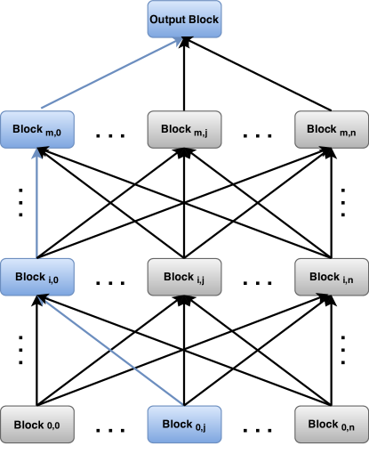
Figure 1: Supernetwork architecture for a generic design. Each block can be a part of neural network, and each connection between sequence of blocks can be a complete architecture. The blue path represent a complete architecture.

4.1 Adaptation to Reinforcement Learning

Most of the existing research on NAS is dedicated to computer vision (particularly, object classification) or computational linguistics applications. We adapt the existing one-shot NAS methods to reinforcement learning. One-shot methods assume the supernetwork which contain all the architectures from the search space as its subgraphs (fig. 1). All the architectures share weights of some of the blocks. That is, each layer in the supernetwork $i$ has a list of $Block_{i}$ options, only one option can be selected for a particular subnetwork. Such simplification was proposed to reduce the co-adaptation between blocks. The whole search space is $\mathcal{A}=Block_{0}\times\ldots\times Block_{n}$. Some initial or final layers of the supernetwork can be fixed and not contain choice blocks.

One-shot methods typically contain a fitting stage. During the fitting stage, the subnetwork $\alpha\in\mathcal{A}$ is sampled by some rule and its weights $\Theta(\alpha)$ are updated by a SGD-like step for a batch of data $B$

$$\Theta(\alpha)\leftarrow\Theta(\alpha)-\eta\nabla_{\Theta(\alpha)}\sum_{i\in B}\ell(y_{i},N(\alpha,\Theta(\alpha),x_{i})),$$ (1)

where $\ell(\cdot)$ is the loss function, $N(\alpha,\theta,x_{i})$ is the network of the architecture $\alpha$ having weights $\Theta(\alpha)$. The evaluation of the architecture $\alpha$ typically involves calculation of performance (accuracy) on the validation dataset $D_{val}$

$$\frac{1}{|D_{val}|}\sum_{i\in D_{val}}[y_{i}=N(\alpha,\Theta(\alpha),x_{i})].$$ (2)

We adapt one-shot methods to RL in the following way. In our experiments, the neural network $N(\alpha,\Theta(\alpha),x_{i})$ corresponds to a policy $\pi_{\Theta(\alpha)}$. Instead of SGD-like step (1) we do the step of PPO

$$\Theta(\alpha)\leftarrow\Theta(\alpha)-\eta\nabla_{\Theta(\alpha)}J^{PPO}_{\Theta(\alpha)}.$$ (3)

The performance of the network is estimated by $\mathbb{E}_{t}[R_{t}[\pi_{\Theta(\alpha)}]$ instead of (2).

4.2 Efficient Neural Architecture Search (ENAS)

Figure 2: A general framework of Neural Architecture Search (NAS)

Efficient Neural Architecture Search (ENAS) [28] is a NAS method, used in our experiments to find a well-performing neural network in the ATARI games environment. ENAS consists of a controller, which samples child models, a search strategy and an evaluation strategy.

In the case of ENAS, the controller is an LSTM network that outputs a one-hot-encoded architecture of a child model. The controller’s inputs are the previous step’s architecture and the reward it has received. The possible choices for a set of child architectures are determined by the search space. The particular variants of the search spaces that we have used are covered in section 5.2.

The authors of [28, 43] have proposed to train an ENAS controller by using RL. In our experiments, we have employed a REINFORCE algorithm, which has also been used in the original paper to update the controller’s network parameters.

In the original paper, due to the different nature of the problems ENAS has been tested on, the child networks, sampled by the controller, are trained until convergence. However, this becomes difficult when the RL environments are considered – the agents usually require longer training times, and the stochasticity of the environments makes the training process much more unpredictable. In our work, we will demonstrate that despite the aforementioned problems, the number of child training timesteps, chosen for our experiments, is still sufficient to determine which networks are better-performing than others.

Finally, the overall sequence of “sampling a child architecture - training a child model - feeding the resulting reward to LSTM controller” (see fig. 2) defines a single epoch of ENAS training. In the previous works on iterative RL NAS methods [43, 44], the fact that such an epoch will take a long time to compute, has limited these methods’ practicality in regard to the real-life problems. The authors of ENAS, however, have come up with the solution to this problem by sharing the weights of all of the child models. This way, the ENAS becomes much more efficient than its predecessors, and, therefore, much more suitable for RL problems.

4.3 Single-Path One-Shot with Uniform Sampling (SPOS)

The method “Single-path one-shot with uniform sampling” was proposed in [15]. The SPOS method assumes two steps: 1) supernetwork fitting 2) best architecture selection. The distinctive feature of SPOS is that subnetworks are sampled from the supernetwork uniformly at random.

Thus, weights $\Theta^{*}$ of the supernetwork are the solution of the following problem

$$\Theta^{*}=\mathop{\mathrm{argmin}}_{\Theta}\mathbb{E}_{\alpha\sim P}[L_{train}(N(\alpha,\Theta(\alpha)))],$$

where $L_{train}(\cdot)$ is the train loss, $P$ - the uniform distribution. During the architecture selection phase, the best subnetwork $\alpha^{*}$ is selected by the validation accuracy $Acc_{val}$

$$\alpha^{*}=\mathop{\mathrm{argmax}}_{\alpha\in\mathcal{A}}Acc_{val}(N(\alpha,\Theta^{*}(\alpha))).$$ (4)

This step requires only inference for the validation data. In the original paper [15], an evolutionary optimization was used to solve (4) since the search space was huge. Instead of evolutionary optimization, we do the full search since our search spaces are small.

The adaptation of SPOS to RL is done as described in the Section 4.1. The subnetwork $N(\alpha,\Theta(\alpha))$ corresponds to a policy $\pi_{\Theta(\alpha)}$. Thus, SPOS for optimizing the neural architecture of the RL agent solves the following problem

$$\Theta^{*}=\mathop{\mathrm{argmax}}_{\Theta}\mathbb{E}_{\alpha\sim P}\mathbb{E}_{t}[R_{t}[\pi_{\Theta(\alpha)}]],$$ (5)

$$\alpha^{*}=\mathop{\mathrm{argmax}}_{\alpha\in\mathcal{A}}\mathbb{E}_{t}[R_{t}[\pi_{\Theta^{*}(\alpha)}].$$ (6)

5 Experiments

5.1 Atari Environment

In our experiments, we used the Open AI Gym framework [5], particularly – Breakout and Freeway Atari environments. We chose the Breakout because it’s a popular benchmark, having moderate standard deviation of RL agent’s reward ($401.2\pm 26.9$, [26]). In opposite to the Breakout, the Freeway environment has very low relative standard deviation of reward ($30.3\pm 0.7$, [26]). The reward of RL agent with random behavior for Breakout and Freeway is nearly zero so we can make sure that our policy network makes non-stochastic behavior.

We have trained the child networks in the manner described in [12], i.e., we have used 8 agents, sharing a policy, trained simultaneously in 8 environments with PPO, in order to collect the trajectories for the policy update. Each of these agents is trained for 128 steps. After that, the controller collects the architecture’s rewards. The controller’s policy is updated every ten steps using the REINFORCE algorithm. Overall, the number of training steps for one experiment equals 10 million. More implementation details are in Appendix C.

It is important to note that the ’scratch’ experimental results demonstrate lower reward values than the ones reported in the original PPO paper [31]. This is due to the fact that in our experiments we have used a smaller number of training timesteps than the classical version of PPO (10M vs. 40M). The reason for this has been that the main aim of our research focuses on investigating whether NAS has a positive effect on RL training process overall, and not on beating the existing ATARI baselines.

5.2 Search Spaces

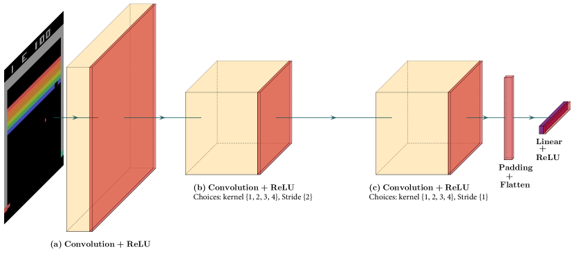
(a) Search space 1: Block(a): fixed kernel size:8, fixed stride:4; Block(b) and Block(c): kernel size is chosen between 1, 2, 3, 4, and 5, and fixed stride: 2, 1 respectively.

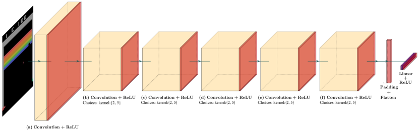
(b) Search space 2: Block(a): fixed kernel size:8, fixed stride:4; Block(b)- Block(f): kernel size is chosen between 2 and 5, with fixed stride: 1 for all of them.

Figure 3: Search spaces used in experiments.

The search spaces that we designed are the extension of the Nature-CNN architecture [26], where convolutional layers are followed by a linear layer which outputs the number of values equal to the size of our action space [26].

In order to facilitate the varying sizes of the layers’ parameters and, hence, enable the weight sharing, we use the following techniques in the overall design of the network:

1. Convolution and max-pooling to the same size: Map the input to one size every time after each convolutional and max-pooling layer.

2. Padding to exact size: Map the output of the last convolutional layer to the target size to be able to fix it during the flattening of the convolutions.

In our experiments we have covered two architectural search spaces:

Search space 1: 25 architectures. The architecture starts with a fixed convolutional layer with input channels equal to 4, and the output channels - to 32, kernel size - 8 and moving stride - 4. This layer is followed by two convolutional layers with output channels equal to 64 per each and with strides 1 and 2. The choices for kernel sizes are 1, 2, 3, 4, 5. The size of this search space is $5^{2}$.

Search space 2: 32 architectures. Instead of two convolutional layers (we do not take into account the first fixed convolutional layer, as we do not vary its kernel size) used in the search space 1, we have used 5 convolutional layers with output channels equal to 64, moving strides equal to 1. The choices for kernels are 2 and 5, which makes the size of this search space equal to $2^{5}$.

The experimental architecture spaces that we have used can be seen in Figure 3(a) and Figure 3(b), and also in Appendix A. The search spaces do not contain very deep architectures, having depth 7 at most.

5.3 Methodology

Firstly, we trained all the architectures from scratch (implementation details are in Appendix C). For all of those architectures we saved mean reward and total reward averaged over last 100 episodes. These metrics were used as a tabular benchmark, eliminating the need to train the same architecture multiple times. We used these metrics later to compare the performances of the found architectures by various NAS methods.

Both NAS methods under evaluation (ENAS, SPOS) share the same high-level structure:

1. Run neural architecture search method for the given search space $\mathcal{A}$;

2. Select top-K architectures from the search space $\mathcal{A}$ by a proxy performance;

3. Train these top-K architectures from scratch;

4. Return the best one by the true performance.

In our experiments, we selected top-3 architectures for the methods under evaluation. We repeated the search 4 times with different seeds and averaged results.

The proxy performance is a part of the NAS method, and it is fast to calculate. The calculation time of the proxy performance is negligible to the time of RL agent training from scratch. For ENAS, the proxy performance of an architecture is the probability of sampling this architecture by the controller. For SPOS, the proxy performance of an architecture is calculated from weights of this architecture in the supernetwork. Namely, the proxy performance is the mean reward of an agent with corresponding weights.

The true performance is the total/mean reward of an RL agent trained from scratch.

5.4 Random search baseline

As a simple baseline, we used the following random search algorithm:

1. Select K architectures from the search space $\mathcal{A}$ at random;

2. Train these K architectures from scratch;

3. Return the best one by the true performance.

As for ENAS and SPOS, we selected top-3 architectures. The only difference with ENAS/SPOS methods is that architectures are selected at random instead of by proxy performance. We estimated the variance of the random search by repeating it for 1000 times.

5.5 Experiments with larger search spaces

We have also tried to expand the search space by increasing the number of consecutive convolutional layers up to 9 and choosing a suitable kernel size and a number of output channels for each of them. However, the results were close to the ones received by random search, which can be caused by the fact that NAS can experience problems with increasingly complex search spaces. For that reason, we do not present the results of these experiments in the paper.

Table 1: Reward mean and total reward of RL agents with various architectures. Each score is the mean of last 100 episodes.

		Search space 1		Search space 2
		Breakout	Freeway	Breakout	Freeway
Random Search	reward mean	54.7 $\pm$ 8.3	28.4 $\pm$ 1.0	33.1 $\pm$ 29.5	21.6 $\pm$ 0.2
	total reward	147.2 $\pm$ 25.5	31.7 $\pm$ 0.8	105.7 $\pm$ 94.2	22.0 $\pm$ 0.2
Nature-CNN [26],	reward mean	57.1	13.1	-	-
reproduced	total reward	157.9	19.0	-	-
ENAS	reward mean	61.4 $\pm$ 1.8	26.4 $\pm$ 1.1	30.7 $\pm$ 21.7	21.5 $\pm$ 0.1
	total reward	161.1 $\pm$ 9.8	30.7 $\pm$ 1.3	91.4 $\pm$ 64.4	22.0 $\pm$ 0.2
SPOS	reward mean	39.7 $\pm$ 18.6	29.6 $\pm$ 0.8	39.9 $\pm$ 41.0	21.7 $\pm$ 0.1
	total reward	144.4 $\pm$ 55.0	29.4 $\pm$ 5.0	180.6 $\pm$ 72.5	22.0 $\pm$ 0.1

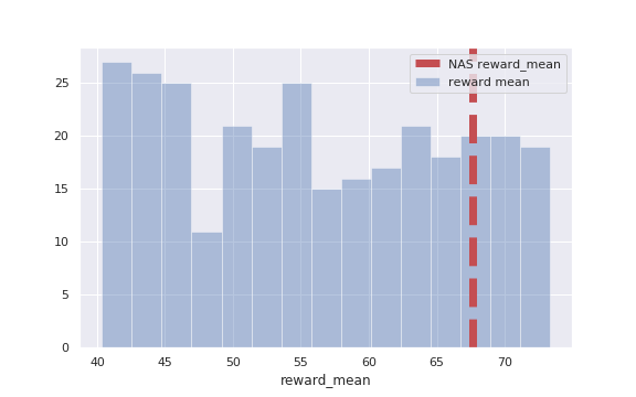
(a) Search Space 1: Breakout

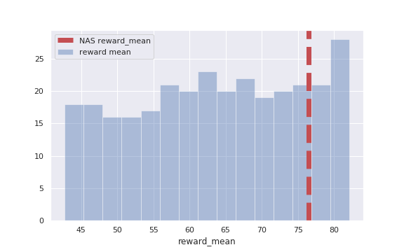
(b) Search Space 2: Breakout

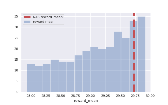
(c) Search Space 1: Freeway

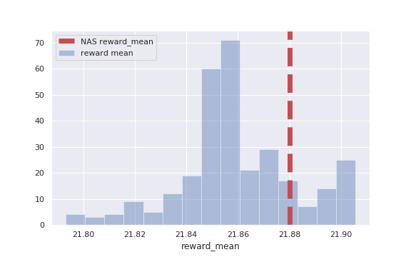
(d) Search Space 2: Freeway

Figure 4: Histograms for the reward mean of RL agents having different architectures from search spaces. The red vertical line depicts the best architecture found by NAS methods.

6 Discussion

Table 1 shows the results of our experiments. For the Breakout environment, ENAS performs better than random search on the search space 1, while SPOS performs better on the search space 2. For the Freeway environment, there is no clear benefit of NAS methods. Variance of the both of the methods are quite high. At the same time, SPOS is simpler since it does not contain an auxiliary controller network.

It is interesting to compare the performances of found architectures with the performance of manually selected Nature-CNN architecture [26] (see description in the Appendix B). The Nature-CNN architecture belongs to the search space 1. For the fair comparison, in Table 1, we report the rewards after training of the Nature-CNN architecture with our pipeline (Section 5.1). The architectures found by NAS methods outperform the manually selected Nature-CNN by a considerable margin.

The existing research on RL methods typically uses the same architectures for different environments. However, we found that this is not optimal. Different architectures are optimal for different environments, see Appendix D.

Figure 4 shows histograms of RL agents’ mean rewards from different search spaces. The red vertical lines depict the best architecture found by NAS methods. We conclude that NAS methods can find top architectures in both of the search spaces.

7 Conclusion

Traditionally, the progress in RL field came mostly from the development of new methods. Neural architectures of RL agents remained relatively simple when compared to computer vision applications.

In this paper, we have applied modern neural architecture search methods for optimizing the architecture of RL agents. We have evaluated ENAS [44] and SPOS [15] methods. Both of them found better architectures than manually picked by experts. We suppose that many RL application can benefit from using better neural architectures. Testing NAS methods for larger search spaces is an interesting topic for further research.

Acknowledgments

Authors are thankful to Mikhail Konobeeb.

8 Appendix

Appendix A Search Spaces

Table 2 describes two search spaces that we used in our experiments. An abbreviation {$1,...,n$} means that a parameter can vary from 1 to $n$ in a search space.

Search Space 1 Layer input output kernel stride Conv-1 $4$ $32$ $8$ $4$ Conv-2 $32$ $64$ $1,..,5$ $2$ Conv-3 $64$ $64$ $1,..,5$ $1$ Padding $-$ $121*64$ $-$ $-$ Linear $121*64$ $512$ $-$ $-$

Search Space 2 Layer input output kernel stride Conv-1 $4$ $32$ $8$ $4$ Conv-2 $32$ $64$ $2,5$ $1$ Conv-3 $64$ $64$ $2,5$ $1$ Conv-4 $64$ $64$ $2,5$ $1$ Conv-5 $64$ $64$ $2,5$ $1$ Conv-6 $64$ $64$ $2,5$ $1$ Padding $-$ $121*64$ $-$ $-$ Linear $121*64$ $512$ $-$ $-$

Table 2: Detailed description of the search spaces.

Appendix B Nature CNN architecture

Table 3 describes the architecture “Nature CNN” [26] which is a member of the search space 1.

Layer	input	output	kernel	stride
Conv-1	$4$	$32$	$8$	$4$
Conv-2	$32$	$64$	$4$	$2$
Conv-3	$64$	$64$	$3$	$1$
Padding	$-$	$121*64$	$-$	$-$
Linear	$121*64$	$512$	$-$	$-$

Table 3: Convolution network architecture that used in [26] that’s contain 3 convolution layer followed by flatten and linear layers.

Appendix C Implementation details

In this section, we present the hyperparameters used for training the RL agents in the ATARI games environment (Table 4), as well as the hyperparameters used for ENAS and SPOS (Table 5). We use the same set of parameters for both training from scratch experiments, and training the child networks sampled by the NAS controllers.

Hyperparameter’s name	Value
# timesteps	$10$M
# runner timesteps	$128$
$\epsilon$ (PPO)	$0.1$
value loss coef. (PPO)	$0.25$
$\lambda$ (GAE)	$0.95$
entropy coef.	$0.01$
learning rate	CosineAnnealing($0.00025$)
# parallel env.	$8$

Table 4: The hyperparameters for training PPO agents on ATARI games.

Hyperparameter’s name	Value
# child network epochs	$10$
# NAS runner timesteps	$3$
NAS entropy coef.	$0.0001$
NAS learning rate	CosineAnnealing($0.001$)
baseline momentum.	$0.2$

Table 5: The hyperparameters for ENAS training.

Appendix D The best architectures

Tables 6, 7, 8, 9 show the best architectures for each game. The architectures tend to be similar for both of the search spaces except the kernel size for the last layers.

Layer	input	output	kernel	stride
Conv-1	$4$	$32$	$8$	$4$
Conv-2	$32$	$64$	$4$	$2$
Conv-3	$64$	$64$	$5$	$1$
Padding	$-$	$121*64$	$-$	$-$
Linear	$121*64$	$512$	$-$	$-$

Table 6: The best architecture for Breakout extracted from search space 1 by SPOS using reward mean criteria.

Layer	input	output	kernel	stride
Conv-1	$4$	$32$	$8$	$4$
Conv-2	$32$	$64$	$3$	$2$
Conv-3	$64$	$64$	$2$	$1$
Padding	$-$	$121*64$	$-$	$-$
Linear	$121*64$	$512$	$-$	$-$

Table 7: The best architecture for Freeway extracted from search space 1 by SPOS using reward mean criteria.

Layer	input	output	kernel	stride
Conv-1	$4$	$32$	$8$	$4$
Conv-2	$32$	$64$	$5$	$1$
Conv-3	$64$	$64$	$5$	$1$
Conv-4	$64$	$64$	$5$	$1$
Conv-5	$64$	$64$	$2$	$1$
Conv-6	$64$	$64$	$2$	$1$
Padding	$-$	$121*64$	$-$	$-$
Linear	$121*64$	$512$	$-$	$-$

Table 8: The best architecture for Breakout extracted from search space 2 by SPOS using reward mean criteria.

Layer	input	output	kernel	stride
Conv-1	$4$	$32$	$8$	$4$
Conv-2	$32$	$64$	$5$	$1$
Conv-3	$64$	$64$	$5$	$1$
Conv-4	$64$	$64$	$5$	$1$
Conv-5	$64$	$64$	$5$	$1$
Conv-6	$64$	$64$	$5$	$1$
Padding	$-$	$121*64$	$-$	$-$
Linear	$121*64$	$512$	$-$	$-$

Table 9: The best architecture for Freeway extracted from search space 2 by SPOS using reward mean criteria.

References

- [1] George Adam and Jonathan Lorraine “Understanding neural architecture search techniques” In arXiv preprint arXiv:1904.00438, 2019
- [2] Richard Bellman “On the theory of dynamic programming” In Proceedings of the National Academy of Sciences of the United States of America 38.8 National Academy of Sciences, 1952, pp. 716
- [3] Gabriel Bender “Understanding and simplifying one-shot architecture search”, 2019
- [4] Konstantinos Bousmalis et al. “Using simulation and domain adaptation to improve efficiency of deep robotic grasping” In 2018 IEEE international conference on robotics and automation (ICRA), 2018, pp. 4243–4250 IEEE
- [5] Greg Brockman et al. “OpenAI Gym” In ArXiv abs/1606.01540, 2016
- [6] Han Cai, Ligeng Zhu and Song Han “Proxylessnas: Direct neural architecture search on target task and hardware” In arXiv preprint arXiv:1812.00332, 2018
- [7] Xin Chen, Lingxi Xie, Jun Wu and Qi Tian “Progressive differentiable architecture search: Bridging the depth gap between search and evaluation” In Proceedings of the IEEE International Conference on Computer Vision, 2019, pp. 1294–1303
- [8] Prafulla Dhariwal et al. “OpenAI Baselines” In GitHub repository GitHub, https://github.com/openai/baselines, 2017
- [9] Xuanyi Dong and Yi Yang “Nas-bench-102: Extending the scope of reproducible neural architecture search” In arXiv preprint arXiv:2001.00326, 2020
- [10] Xuanyi Dong and Yi Yang “Searching for a robust neural architecture in four gpu hours” In Proceedings of the IEEE Conference on Computer Vision and Pattern Recognition, 2019, pp. 1761–1770
- [11] Thomas Elsken, Jan Hendrik Metzen and Frank Hutter “Efficient multi-objective neural architecture search via lamarckian evolution” In arXiv preprint arXiv:1804.09081, 2018
- [12] Lasse Espeholt et al. “Impala: Scalable distributed deep-rl with importance weighted actor-learner architectures” In arXiv preprint arXiv:1802.01561, 2018
- [13] Federico Girosi, Michael Jones and Tomaso Poggio “Regularization Theory and Neural Networks Architectures”, 1995 DOI: 10.1162/neco.1995.7.2.219
- [14] Shixiang Gu, Ethan Holly, Timothy Lillicrap and Sergey Levine “Deep reinforcement learning for robotic manipulation with asynchronous off-policy updates” In 2017 IEEE international conference on robotics and automation (ICRA), 2017, pp. 3389–3396 IEEE
- [15] Zichao Guo et al. “Single path one-shot neural architecture search with uniform sampling” In arXiv preprint arXiv:1904.00420, 2019
- [16] Kirthevasan Kandasamy et al. “Neural architecture search with bayesian optimisation and optimal transport” In Advances in Neural Information Processing Systems, 2018, pp. 2016–2025
- [17] Steven Kapturowski et al. “Recurrent Experience Replay in Distributed Reinforcement Learning” In International Conference on Learning Representations, 2019 URL: https://openreview.net/forum?id=r1lyTjAqYX
- [18] Nikita Klyuchnikov et al. “NAS-Bench-NLP: Neural Architecture Search Benchmark for Natural Language Processing” In arXiv preprint arXiv:2006.07116, 2020
- [19] Sergey Levine, Aviral Kumar, George Tucker and Justin Fu “Offline reinforcement learning: Tutorial, review, and perspectives on open problems” In arXiv preprint arXiv:2005.01643, 2020
- [20] Liam Li and Ameet Talwalkar “Random search and reproducibility for neural architecture search” In arXiv preprint arXiv:1902.07638, 2019
- [21] Hanwen Liang et al. “Darts+: Improved differentiable architecture search with early stopping” In arXiv preprint arXiv:1909.06035, 2019
- [22] Marius Lindauer and Frank Hutter “Best practices for scientific research on neural architecture search” In arXiv preprint arXiv:1909.02453, 2019
- [23] Hanxiao Liu, Karen Simonyan and Yiming Yang “Darts: Differentiable architecture search” In arXiv preprint arXiv:1806.09055, 2018
- [24] Sam McCandlish, Jared Kaplan, Dario Amodei and OpenAI Dota Team “An empirical model of large-batch training” In arXiv preprint arXiv:1812.06162, 2018
- [25] Volodymyr Mnih et al. “Asynchronous methods for deep reinforcement learning” In International conference on machine learning, 2016, pp. 1928–1937
- [26] Volodymyr Mnih et al. “Human-level control through deep reinforcement learning”, 2015, pp. 2–3 DOI: 10.1038/nature14236
- [27] Volodymyr Mnih et al. “Playing atari with deep reinforcement learning” In arXiv preprint arXiv:1312.5602, 2013
- [28] Hieu Pham et al. “Efficient neural architecture search via parameter sharing” In arXiv preprint arXiv:1802.03268, 2018
- [29] Esteban Real, Alok Aggarwal, Yanping Huang and Quoc V Le “Regularized evolution for image classifier architecture search” In Proceedings of the aaai conference on artificial intelligence 33, 2019, pp. 4780–4789
- [30] Julian Schrittwieser et al. “Mastering Atari, Go, Chess and Shogi by Planning with a Learned Model” In ArXiv abs/1911.08265, 2019
- [31] John Schulman et al. “Proximal Policy Optimization Algorithms”, 2017 arXiv:1707.06347 [cs.LG]
- [32] Han Shi et al. “Multi-objective Neural Architecture Search via Predictive Network Performance Optimization” In arXiv preprint arXiv:1911.09336, 2019
- [33] David Silver et al. “Mastering the game of go without human knowledge” In Nature 550.7676 Nature Publishing Group, 2017, pp. 354–359
- [34] Richard S Sutton and Andrew G Barto “Reinforcement learning: An introduction” MIT press, 2018
- [35] Richard S Sutton, David A McAllester, Satinder P Singh and Yishay Mansour “Policy gradient methods for reinforcement learning with function approximation” In Advances in neural information processing systems, 2000, pp. 1057–1063
- [36] Emanuel Todorov, Tom Erez and Yuval Tassa “Mujoco: A physics engine for model-based control” In 2012 IEEE/RSJ International Conference on Intelligent Robots and Systems, 2012, pp. 5026–5033 IEEE
- [37] Ilya Trofimov et al. “Multi-fidelity Neural Architecture Search with Knowledge Distillation” In arXiv preprint arXiv:2006.08341, 2020
- [38] Colin White, Willie Neiswanger and Yash Savani “BANANAS: Bayesian Optimization with Neural Architectures for Neural Architecture Search” In arXiv preprint arXiv:1910.11858, 2019
- [39] R.. Williams “Simple statistical gradient-following algorithms for connectionist reinforcement learning” In Machine Learning, 1992
- [40] Yuhui Xu et al. “Pc-darts: Partial channel connections for memory-efficient differentiable architecture search” In arXiv preprint arXiv:1907.05737, 2019
- [41] Antoine Yang, Pedro M Esperança and Fabio M Carlucci “NAS evaluation is frustratingly hard” In arXiv preprint arXiv:1912.12522, 2019
- [42] Chris Ying et al. “Nas-bench-101: Towards reproducible neural architecture search” In International Conference on Machine Learning, 2019, pp. 7105–7114
- [43] Barret Zoph and Quoc V Le “Neural architecture search with reinforcement learning” In arXiv preprint arXiv:1611.01578, 2016
- [44] Barret Zoph, Vijay Vasudevan, Jonathon Shlens and Quoc V Le “Learning transferable architectures for scalable image recognition” In Proceedings of the IEEE conference on computer vision and pattern recognition, 2018, pp. 8697–8710