Coherences and the thermodynamic uncertainty relation: Insights from quantum absorption refrigerators

Abstract

The thermodynamic uncertainty relation, originally derived for classical Markov-jump processes, provides a trade-off relation between precision and dissipation, deepening our understanding of the performance of quantum thermal machines. Here, we examine the interplay of quantum system coherences and heat current fluctuations on the validity of the thermodynamics uncertainty relation in the quantum regime. To achieve the current statistics, we perform a full counting statistics simulation of the Redfield quantum master equation. We focus on steady-state quantum absorption refrigerators where nonzero coherence between eigenstates can either suppress or enhance the cooling power, compared with the incoherent limit. In either scenario, we find enhanced relative noise of the cooling power (standard deviation of the power over the mean) in the presence of system coherence, thereby corroborating the thermodynamic uncertainty relation. Our results indicate that fluctuations necessitate consideration when assessing the performance of quantum coherent thermal machines.

I Introduction

Quantum thermodynamics is an emerging research field concerning the thermodynamics and nonequilibrium statistical mechanics of open quantum nanoscale systems with the full inclusion of quantum effects Scovil and Schulz-DuBois (1959); Geva and Kosloff (1992a); Gemmer et al. (2009); Seifert (2012); Pekola (2015); Kosloff (2013); Goold et al. (2016); Vinjanampathy and Anders (2016); Binder et al. (2018); Seifert (2019); Pekola and Khaymovich (2019). In the quantum realm, basic notions such as heat and work of classical thermodynamics need to be reexamined and refined (see for example, Refs. Talkner et al. (2007); Talkner and Hänggi (2016, 2020)), leading to, for instance, intriguing microscopic unravelling of the second law of thermodynamics Esposito et al. (2009); Campisi et al. (2011).

A tantalizing prospect of the field of quantum thermodynamics is to devise and realize quantum thermal machines (QTMs) that transform heat to useful work or use work to refrigerate Scovil and Schulz-DuBois (1959); Alicki (1979); Geva and Kosloff (1992b); Giazotto et al. (2006); Filliger and Reimann (2007); Esposito et al. (2010); Linden et al. (2010); Seifert (2012); Levy and Kosloff (2012); Abah et al. (2012); Blickle and Bechinger (2012); Kosloff and Levy (2014); Roßnagel et al. (2014); Thierschmann et al. (2015); Dechant et al. (2015); Harris (2016); Robnagel et al. (2016); Uzdin et al. (2015); Hofer et al. (2016a, b); Zou et al. (2017); Martinez et al. (2016); Ghosh et al. (2017); Klaers et al. (2017); Elouard et al. (2017); Abah and Lutz (2017); Benenti et al. (2017); Ronzani et al. (2018); Josefsson et al. (2018); Friedman et al. (2018); Kilgour and Segal (2018); Elouard and Jordan (2018); Pietzonka et al. (2019); de Assis et al. (2019); Mitchison (2019); Peterson et al. (2019); Klatzow et al. (2019); von Lindenfels et al. (2019); Buffoni et al. (2019); Abiuso and Perarnau-Llobet (2020); Carollo et al. (2020); Hartmann et al. (2020); Van Horne et al. (2020); Ono et al. (2020); Bhandari et al. (2020). Efficient QTMs, capable of exploiting genuine quantum effects and outperforming their classical counterparts, are of paramount importance for future quantum technologies. In this regard, the discussion of whether quantum coherence can be an advantageous resource in the operation of QTMs is an ongoing and vivid topic of this field Scully et al. (2003); Zhang et al. (2007); Dillenschneider and Lutz (2009); Scully et al. (2011); Dorfman et al. (2013); Rahav et al. (2012); Killoran et al. (2015); Leggio et al. (2015); Niedenzu et al. (2015); Gelbwaser-Klimovsky et al. (2015); Brandner et al. (2015); Mitchison et al. (2015); Uzdin et al. (2015); Su et al. (2016); Türkpençe and Müstecaplıoğlu (2016); Uzdin (2016); Mehta and Johal (2017); Chen et al. (2017); Holubec and Novotný (2018); Kilgour and Segal (2018); Wertnik et al. (2018); Holubec and Novotný (2019); Latune et al. (2019, 2020); Francica et al. (2020).

At the nanoscale, fluctuations become significant, implying that one should inspect nonequilibrium fluctuations of thermodynamic quantities for characterizing the performance of QTMs Verley et al. (2014); Seifert (2012); Rahav et al. (2012); Esposito et al. (2015); Agarwalla et al. (2015); Polettini et al. (2015); Jiang et al. (2015); Campisi et al. (2015); Campisi and Fazio (2016); Holubec and Ryabov (2017); Segal (2018); Friedman and Segal (2019); Friedman et al. (2018); Holubec and Ryabov (2018); Manikandan et al. (2019); Vroylandt et al. (2020). Recently, a conceptual advance, termed thermodynamic uncertainty relation (TUR) Barato and Seifert (2015); Gingrich et al. (2016); Horowitz and Gingrich (2019), is offering new insights into the characteristics of steady-state QTMs in terms of a trade-off relation between power fluctuation and efficiency Pietzonka and Seifert (2018). While the original TUR was derived for systems described by classical Markov jump processes, quantum generalizations of TURs have been conceived for steady-state Guarnieri et al. (2019) and cyclic Miller et al. (2020) QTMs. To assess the performance of QTMs, it is necessary to explore how quantum effects such as coherence contribute to the relative noise and to the behavior of the TUR Ptaszyński (2018); Agarwalla and Segal (2018); Liu and Segal (2019); Rignon-Bret et al. (2020); Cangemi et al. (2020).

Here, we focus on models for a quantum absorption refrigerator (QAR), a steady-state QTM that continuously pumps heat from a cold bath into a hot bath by consuming power from a (very hot) ‘work’ bath. The study of QAR developed from early studies of a three-level maser, an engine Scovil and Schulz-DuBois (1959). With rapid developments in quantum thermodynamics, recent years have witnessed a great number of investigations on various aspects of QARs Linden et al. (2010); Brunner et al. (2012); Levy and Kosloff (2012); Correa et al. (2013); Kosloff and Levy (2014); Correa et al. (2014a, 2015); Hofer et al. (2016b); Mitchison et al. (2016); Mu et al. (2017); González et al. (2017); Segal (2018); Correa et al. (2014b); Mitchison (2019). Despite significant progress on the subject, the interplay of coherence and fluctuation in the performance of QARs remains largely unexplored, although studies have revealed the pros and cons of system coherence on cooling power Kilgour and Segal (2018); Holubec and Novotný (2018); Mitchison (2019).

Focusing on QARs in which the system coherence was shown to have a nontrivial effect on the cooling power Kilgour and Segal (2018); Holubec and Novotný (2018, 2019), the objectives of the present study are twofold: (i) We aim to identify the role of steady state system coherence (between system energy eigenstates) on power fluctuations. If system coherences are systematically linked to reduced fluctuations, they become a useful resource for QARs if the net power is instead enhanced. Conversely, if fluctuations consistently increase when system coherences exist (compared to the incoherent limit), then power boost associated with coherences may not be profitable. (ii) We aim to test the behavior of the TUR ratio (relative noise times entropy production) Barato and Seifert (2015); Gingrich et al. (2016); Guarnieri et al. (2019) in the presence of system coherences. Can coherences improve this trade-off relation, i.e. allow the system to operate closer to the bound relative to the incoherent scenario?

To attain the heat current and its noise, we combine a full counting statistics formalism Levitov and Lesovik (1993); Levitov et al. (1996) within the Redfield master equation (RME) Redfield (1957, 1965). The method is perturbative in the system-bath coupling, but allows arbitrarily strong internal system’s coherences.

We confirm the thermodynamic consistency of the method by validating the fluctuation symmetry for heat transfer Esposito et al. (2009); Campisi et al. (2011). To demonstrate the nontrivial role of system coherences on the cooling current and its fluctuations, we compare results under the full Redfield calculations with those obtained in the incoherent limit where coherences vanish. We find that system coherences always enhance the relative noise of the cooling power compared with the incoherent limit, despite that it can either suppress or enhance the cooling power itself. Particularly, considering a model for a QAR where system coherences enhance the cooling power Holubec and Novotný (2018), we show that power fluctuations get amplified as well, indicating that system coherences are not helpful in terms of constancy Pietzonka and Seifert (2018).

As a result of the enhanced relative noise, the TUR is always satisfied by the QARs under investigation here—regardless of the presence of system coherences. Our results thus suggest that violations of TUR observed in steady-state QTMs at weak couplings Ptaszyński (2018); Agarwalla and Segal (2018); Liu and Segal (2019) should not be attributed to nonzero system coherences.

The paper is organized as follows. In Sec. II, we first introduce the general setup and the counting-field dressed Redfield master equation. We then briefly mention how to get currents and fluctuations from the cumulant generating function and demonstrate the thermodynamic consistency of the Redfield master equation by validating the fluctuation symmetry for a V-shaped system. In Sec. III, we focus on two concrete examples of steady-state QARs and provide detailed simulation results for the cooling current, its fluctuations, and the TUR. We conclude in Sec. IV.

II Model and methodology

In this section, we first introduce the general modeling of QTMs as open quantum systems connected to multiple heat baths. We then lay out the counting-field dressed Redfield master equation ($\chi-$ RME) for the sake of completeness and present expressions for currents and fluctuations from the cumulant generating function. Finally, we check the thermodynamic consistency of the counting-field dressed Redfield master equation by verifying the fluctuation symmetry of heat exchange for the V-shaped system. The behavior of the heat current and coherences in the V-shaped system closely relate to the cooling characteristics of our model I [see Fig. 4 (a)] for a QAR Kilgour and Segal (2018). As such, verifying the fluctuation symmetry of heat exchange for the V-shaped system indicates on the corresponding behavior for QARs.

II.1 Hamiltonian for QTMs

QTMs can be modeled as open quantum systems consisting of a central system ($s$) coupled to multiple (counted by $v$) bosonic heat baths ($b$). The total system-bath Hamiltonian reads (setting $\hbar=1$ and $k_{B}=1$ hereafter)

$$\hat{H}\leavevmode\nobreak\ =\leavevmode\nobreak\ \hat{H}_{s}+\sum_{v}\hat{H}_{b}^{v}+\hat{H}_{sb},\leavevmode\nobreak\ \leavevmode\nobreak\ \leavevmode\nobreak\ \hat{H}_{sb}\leavevmode\nobreak\ =\leavevmode\nobreak\ \sum_{v}\hat{S}_{v}\otimes\hat{B}_{v}.$$ (1)

Here and in what follows, we imply the tensor product with the identity so that $\hat{H}_{s}$ will be used instead of $\hat{H}_{s}\otimes\mathbb{I}_{b}$ with $\mathbb{I}_{b}$ an identity matrix in the bath subspace and so on. The working substance $\hat{H}_{s}$ constitutes a few-level quantum system. The bosonic heat baths are assumed to be harmonic,

$$\hat{H}_{b}^{v}\leavevmode\nobreak\ =\leavevmode\nobreak\ \sum_{k}\omega_{kv}\hat{b}_{kv}^{\dagger}\hat{b}_{kv},$$ (2)

with $\hat{b}_{kv}^{\dagger}$ ($\hat{b}_{kv}$) creating (annihilating) a harmonic mode $k$ with frequency $\omega_{kv}$ in $v$ bath. Here, we assume that each bath is described by a thermal equilibrium state characterized by a temperature $T_{v}$. $\hat{S}_{v}$ and $\hat{B}_{v}$ are system and reservoir operators that form the coupling between the system and $v$ bath, respectively. We consider bilinear system-bath interactions and take $\hat{B}_{v}$ to be the displacement operators,

$$\hat{B}_{v}\leavevmode\nobreak\ =\leavevmode\nobreak\ \sum_{k}\lambda_{kv}(\hat{b}_{kv}^{\dagger}+\hat{b}_{kv})$$ (3)

with $\lambda_{kv}$ characterizing the coupling strength between the system and the $v$ reservoir.

II.2 Counting-field dressed Redfield master equation

To study the thermodynamics of the generic QTMs defined above, we combine the full counting statistic formalism Levitov and Lesovik (1993); Levitov et al. (1996) with the Redfield master equation Redfield (1957, 1965). This formalism was recently described in details in Ref. Friedman et al. (2018). To do so, we assign each bath a counting field $\chi_{v}$. The moment generating function is defined with the two-time measurement protocol as Esposito et al. (2009)

$$\mathcal{Z}(\{\chi_{v}\},t)\leavevmode\nobreak\ \equiv\leavevmode\nobreak\ {\rm Tr}\left[e^{i\sum_{v}\chi_{v}\hat{H}_{b}^{v}(0)}e^{-i\sum_{v}\chi_{v}\hat{H}_{b}^{v}(t)}\hat{\rho}(0)\right].$$ (4)

Here, operators are written in the Heisenberg picture. $\hat{\rho}(0)$ denotes the initial factorized density matrix of the system (s) and bath (b), $\hat{\rho}(0)=\hat{\rho}_{s}(0)\otimes\hat{\rho}_{b}(0)$; $\hat{\rho}_{b}(0)=\prod_{v}\exp(-\beta_{v}\hat{H}_{v})/Z_{v}$ with $\beta_{v}=T_{v}^{-1}$ and $Z_{v}$ the inverse temperature and partition function for the $v$ bath, respectively. After some simple manipulations, we arrive at Friedman et al. (2018)

$$\mathcal{Z}(\{\chi_{v}\},t)\leavevmode\nobreak\ =\leavevmode\nobreak\ \mathrm{Tr}[\hat{\rho}^{\chi}(t)],$$ (5)

where the counting-field dressed total density matrix reads

$$\hat{\rho}^{\chi}(t)\leavevmode\nobreak\ \equiv\leavevmode\nobreak\ \hat{U}^{-\chi}(t)\hat{\rho}(0)\hat{U}^{\chi,\dagger}(t);\leavevmode\nobreak\ \leavevmode\nobreak\ \hat{U}^{-\chi}(t)\leavevmode\nobreak\ \equiv\leavevmode\nobreak\ e^{-i\hat{H}^{-\chi}t}$$ (6)

with $\hat{H}^{-\chi}\equiv e^{-i\sum_{v}\chi_{v}\hat{H}_{b}^{v}/2}\hat{H}e^{i\sum_{v}\chi_{v}\hat{H}_{b}^{v}/2}$ denoting the counting-field dressed total Hamiltonian. Notice that we have $[\hat{\rho}^{\chi}]^{\dagger}=\hat{\rho}^{-\chi}$. Equation (6) can be written as a differential equation, generalizing the Liouville Equation for the density matrix (in the Schrödinger picture),

$$\frac{d\hat{\rho}^{\chi}}{dt}=-i\hat{H}^{-\chi}\hat{\rho}^{\chi}(t)+i\rho^{\chi}(t)\hat{H}^{\chi}.$$ (7)

The moment generating function is obtained by solving this equation of motion, then tracing $\hat{\rho}^{\chi}$.

Using the explicit form given by Eq. (1), we get

$$\hat{H}^{-\chi}\leavevmode\nobreak\ =\leavevmode\nobreak\ \hat{H}_{s}+\sum_{v}\hat{H}_{b}^{v}+\sum_{v}\hat{S}_{v}\otimes\hat{B}_{v}^{-\chi_{v}},$$ (8)

where $\hat{B}_{v}^{-\chi_{v}}=e^{-i\chi_{v}\hat{H}_{b}^{v}/2}\hat{B}_{v}e^{i\chi_{v}\hat{H}_{b}^{v}/2}=\sum_{k}\lambda_{kv}(e^{-i\chi_{v}\omega_{kv}/2}\hat{b}_{kv}^{\dagger}+\mathrm{H.c.})$ with ‘H.c.’ denoting Hermitian conjugate hereafter. Proceeding from Eq. (7) in the interaction representation, treating the counting-field dressed system-bath coupling as a perturbation, and then transforming back to the Schrödinger picture, the reduced density matrix dynamics $\rho_{s}^{\chi}(t)\equiv{\rm Tr}_{b}[\rho^{\chi}(t)]$ can be described by the following $\chi$-RME in the energy basis $\{|n\rangle\}$ of $\hat{H}_{s}$ (detailed derivation can be found in, e.g., Ref. Friedman et al. (2018)):

$$\frac{\partial}{\partial t}\rho_{s,nm}^{\chi}(t) = -i\Delta_{nm}\rho_{s,nm}^{\chi}(t)-\sum_{v}\sum_{jk}\Big{[}\mathcal{R}_{mk,kj}^{v,\ast}(\Delta_{jk})\rho_{s,nj}^{\chi}(t)$$ (9)

$$-\mathcal{R}_{nj,km}^{\chi_{v}}(\Delta_{jn})\rho_{s,jk}^{\chi}(t)-\mathcal{R}_{mk,jn}^{-\chi_{v}^{\ast},\ast}(\Delta_{km})\rho_{s,jk}^{\chi}(t)$$

$$+\mathcal{R}_{nj,jk}^{v}(\Delta_{kj})\rho_{s,km}^{\chi}(t)\Big{]}.$$

Here, $\rho_{s,nm}^{\chi}(t)\equiv\langle n|\rho_{s}^{\chi}(t)|m\rangle$, $\Delta_{ij}=E_{i}-E_{j}$ are energy gaps with $E_{i}$ eigenenergies of the subsystem in the global (eigenenergy) basis. The superscript ‘$\ast$’ denotes complex conjugate. The standard Redfield equation is recovered when counting parameters are taken to zero, $\mathcal{R}_{nm,lk}^{v}(\omega)=\left.\mathcal{R}_{nm,lk}^{\chi_{v}}(\omega)\right|_{\chi_{v}=0}$. The transition coefficients satisfy

$$\mathcal{R}_{nm,lk}^{\chi_{v}}(\omega) \equiv S_{v}^{nm}S_{v}^{lk}\int_{0}^{\infty}d\tau e^{i\omega\tau}\Omega_{v}(\chi_{v}+\tau),$$ (10)

with $\Omega_{v}(\tau)\equiv\langle\hat{B}_{v}(\tau)\hat{B}_{v}(0)\rangle_{b}$ denoting the bath correlation function evaluated using the state $\hat{\rho}_{b}(0)$. Its explicit form reads

$$\Omega_{v}(\tau)=\int_{0}^{\infty}d\omega\frac{\gamma_{v}(\omega)}{2\pi}\Big{[}e^{i\omega\tau}n_{B}^{v}(\omega)+e^{-i\omega\tau}\Big{(}1+n_{B}^{v}(\omega)\Big{)}\Big{]}$$

with $\gamma_{v}(\omega)=2\pi\sum_{k}\lambda_{kv}^{2}\delta(\omega-\omega_{kv})$ and $n_{B}^{v}(\omega)$ the spectral density and Bose-Einstein distribution of $v$ bath, respectively. Without loss of generality, here we consider an Ohmic function $\gamma_{v}(\omega)=\alpha_{v}\omega e^{-\omega/\omega_{c}}$; $\alpha_{v}$ is a dimensionless system-bath coupling strength. We assume all baths have the same cutoff frequency $\omega_{c}$, which defines the largest energy scale in the problem.

With Eq. (II.2), we can evaluate the above transition coefficients as $\mathcal{R}_{nm,lk}^{\chi_{v}}(\omega)=S_{v}^{nm}S_{v}^{lk}\Gamma_{\chi_{v}}(\omega)$ with

$$\Gamma_{\chi_{v}}(\omega) \equiv \left\{\begin{array}[]{cc}\gamma_{v}(\omega)e^{-i\omega\chi_{v}}[1+n_{B}^{v}(\omega)]/2&\mathrm{for}\leavevmode\nobreak\ \omega>0,\\ \gamma_{v}(|\omega|)e^{i|\omega|\chi_{v}}n_{B}^{v}(|\omega|)/2&\mathrm{for}\leavevmode\nobreak\ \omega<0.\end{array}\right.$$ (14)

Here, ‘$|A|$’ takes the absolute value of $A$. We neglected the Lamb shifts, which is justified in the weak system-bath coupling limit. To assess the role of nonzero system coherences, we contrast the full $\chi$-RME given by Eq. (9) against its secular counterpart in which coherences between energy eigenstates vanish Friedman et al. (2018),

$$\frac{\partial}{\partial t}\rho_{s,nn}^{\chi}(t) = -\sum_{v}\sum_{k}\Big{[}2\mathrm{Re}\left(\mathcal{R}_{nk,kn}^{v}(\Delta_{nk})\right)\rho_{s,nn}^{\chi}(t)$$ (15)

$$-\mathcal{R}_{nk,kn}^{\chi_{v}}(\Delta_{kn})\rho_{s,kk}^{\chi}(t)$$

$$-\mathcal{R}_{nk,kn}^{-\chi_{v}^{\ast},\ast}(\Delta_{kn})\rho_{s,kk}^{\chi}(t)\Big{]}.$$

Hereafter, we refer to Eq. (15) as the secular $\chi$-RME with the understanding that it represents the incoherent limit of the full $\chi$-RME. Below, we use “secular limit” and “incoherent limit” interchangeably.

To obtain the current and its higher-order cumulants, we recast the $\chi$-RME in the Liouville space as

$$\frac{\partial}{\partial t}|\rho^{\chi}_{s}(t)\rangle\rangle\leavevmode\nobreak\ =\leavevmode\nobreak\ -\mathbb{L}_{\chi}|\rho_{s}^{\chi}(t)\rangle\rangle,$$ (16)

where $|\rho_{s}^{\chi}\rangle\rangle\equiv(\rho_{s,11}^{\chi},\rho_{s,12}^{\chi},\cdots,\rho_{s,nm}^{\chi},\cdots,\rho_{s,NN}^{\chi})^{T}$ denotes an $N^{2}\times 1$ vector with $N$ the dimension of the system Hilbert space. $\mathbb{L}_{\chi}$ is an $N^{2}\times N^{2}$ matrix representing the $\chi$-dependent Liouvillian superoperator (noting that $\mathbb{L}_{\chi}$ reduces to an $N\times N$ matrix in the secular limit). In the steady state limit, the cumulant generating function (CGF) $G(\chi)\leavevmode\nobreak\ =\leavevmode\nobreak\ \lim_{t\to\infty}\ln\mathcal{Z}(\chi,t)/t$ is given by Esposito et al. (2009)

$$G(\chi)\leavevmode\nobreak\ =\leavevmode\nobreak\ -\mathcal{E}_{0}(\chi),$$ (17)

where $\mathcal{E}_{0}(\chi)$ is the ground-state energy (or the eigenvalue of the smallest real part) of the superoperator $\mathbb{L}_{\chi}$. In scenarios with multiple bath, $\chi$ should be understood as a collection of counting fields, namely, $\chi=\{\chi_{v}\}$.

We note that $\mathcal{E}_{0}(0)=0$, that is, without counting the smallest eigenstate is zero, corresponding to the steady state solution. The CGF supplies all cumulants, specifically the steady state heat current $\langle J_{v}\rangle$ out of the $v$th reservoir and its fluctuation $\langle\langle J_{v}^{2}\rangle\rangle\equiv\langle J_{v}^{2}\rangle-\langle J_{v}\rangle^{2}$,

$$\langle J_{v}\rangle = -\left.\frac{\partial\mathcal{E}_{0}(\chi)}{\partial(i\chi_{v})}\right|_{\{\chi_{v}\}=0}$$

$$= -\left.\frac{\mathcal{E}_{0}(\chi_{v})-\mathcal{E}_{0}(-\chi_{v})}{2(i\chi_{v})}\right|_{\chi_{v}\to 0,\{\chi_{v^{\prime}\neq v}\}=0},$$

$$\langle\langle J_{v}^{2}\rangle\rangle = -\left.\frac{\partial^{2}\mathcal{E}_{0}(\chi)}{\partial(i\chi_{v})^{2}}\right|_{\{\chi_{v}\}=0}$$ (18)

$$= \left.\frac{\mathcal{E}_{0}(\chi_{v})+\mathcal{E}_{0}(-\chi_{v})}{\chi_{v}^{2}}\right|_{\chi_{v}\to 0,\{\chi_{v^{\prime}\neq v}\}=0}.$$

Here, $\mathcal{E}_{0}(-\chi)$ is the ground-state energy of $\mathbb{L}_{-\chi}$. In numerical simulations presented below, we adopt a real value of $\chi_{v}=0.001-0.005$ to calculate $\langle J_{v}\rangle$ and $\langle\langle J_{v}^{2}\rangle\rangle$ according to the second lines of the above definitions. We verified that the final results of $\langle J_{v}\rangle$ and $\langle\langle J_{v}^{2}\rangle\rangle$ were independent of the value of $\chi_{v}$ we set.

With the ability to calculate currents and fluctuations, we further study the validity of the thermodynamic uncertainty relation (TUR) Barato and Seifert (2015); Gingrich et al. (2016)

$$\frac{\langle\langle J_{v}^{2}\rangle\rangle}{\langle J_{v}\rangle^{2}}\langle\sigma\rangle\geqslant 2,$$ (19)

with $\langle\sigma\rangle=-\sum_{v}\langle J_{v}\rangle\beta_{v}$ the total entropy production rate. Here we adopt the convention that $\langle J_{v}\rangle>0$ when flowing into the system. In what follows, we refer to the quantity ‘$\frac{\langle\langle J_{v}^{2}\rangle\rangle}{\langle J_{v}\rangle^{2}}\langle\sigma\rangle$’ as the TUR ratio. Note that below we find that our models for QAR always satisfy the original TUR (19). As such, we obviously satisfy the generalized—and less tight bounds as discussed in Refs. Guarnieri et al. (2019); Horowitz and Gingrich (2019).

In sum, in our procedure we construct the Liouvillians $\mathbb{L}_{\chi}$ for both the full Redfield and the secular Redfield equations and find their smallest eigenvalues, the CGF. We obtain the steady state heat current from bath $v$ and the current noise by numerically calculating the first and second derivatives of the CGF, respectively, taken with respect to the counting parameter of bath $v$.

II.3 Verifying the fluctuation symmetry with the $\chi$-RME

Numerous studies in past years had examined the regime of validity and accuracy of second-order Markovian quantum master equations, specifically comparing the Redfield master equation to the local Lindblad master equation (LLME), which is performed in the site basis, and the eigenbasis Lindblad master equation (ELME) Wichterich et al. (2007); Levy and Kosloff (2014); Purkayastha et al. (2016); Hofer et al. (2017); González et al. (2018); Chiara et al. (2018); Cattaneo et al. (2019), which is performed in the global basis. The Redfield equation reduces to the ELME after making the secular approximation. The LLME is derived in the site basis, and it is known to miss proper thermalization further showing incorrect transport properties Levy and Kosloff (2014). Comparing the predictions of the RME to exact results (when available), it has been generally concluded that the RME is superior over both the ELME and the LLME Wichterich et al. (2007); Purkayastha et al. (2016); González et al. (2018).

On the other hand, the Redfield dissipator does not necessarily satisfy the condition of complete positivity (unlike the Lindblad dissipator). How does this deficiency impact thermodynamical properties? To the best of our knowledge, there are no reports on the impact of deviations from complete positivity on steady state behavior. However, for a driven system it was shown in Ref. Argentieri et al. (2014) that the departure from complete positivity lead to the violation of the second law of thermodynamics, with a negative entropy production at intermediate times.

For a system coupled to three baths ($h,w,c$) with no internal leaks, the cumulant generating function satisfies the steady state exchange fluctuation symmetry (SSFS) Esposito et al. (2009); Campisi et al. (2011); Segal (2018); Andrieux et al. (2009); Liu et al. (2018),

$$G(\chi_{c},\chi_{w})\leavevmode\nobreak\ =\leavevmode\nobreak\ G(i(\beta_{h}-\beta_{c})-\chi_{c},i(\beta_{h}-\beta_{w})-\chi_{w}).$$ (20)

A fundamental question that is still not settled is whether the full $\chi$-RME satisfies this relation, thus is consistent with nonequilibrium thermodynamics. The secular limit of the $\chi$-RME, that is the eigenbasis Lindblad master equation, satisfies the SSFS for QAR Segal (2018). On the other hand, if the fluctuations symmetry is not satisfied in the full $\chi$-RME, it is important to find out what is the impact of this deviation on the accuracy of calculated cumulants of transport. In other words, whether this deviation influences the small $\chi$ behavior. This point is critical to our analysis since we are using the $\chi$-RME to calculate the current and its fluctuations under the influence of quantum coherences.

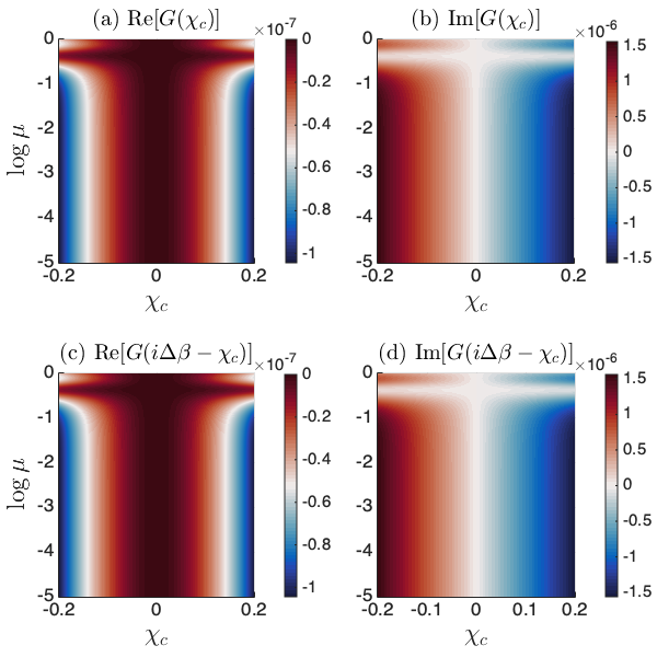
Figure 1: Verifying the steady state exchange fluctuation symmetry, Eq. (21), for the V-shaped system using the secular $\chi$-RME Eq. (15). (a) Real (Re) and (b) imaginary (Im) parts of $G(\chi_{c})$. (c) Real and (d) imaginary part of $G(i\Delta\beta-\chi_{c})$. Other parameters are $\epsilon_{g}=0$, $\epsilon_{e}=0.4$, $\alpha_{h,c}=0.002$, $\omega_{c}=50$, $T_{h}=0.15$ and $T_{c}=0.1$.

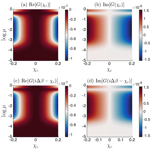
Figure 2: Verifying the steady state exchange fluctuation symmetry Eq. (21) for the V-shaped system using the full $\chi$-RME, Eq. (9). (a) Real (Re) and (b) imaginary (Im) parts of $G(\chi_{c})$. (c) Real and (d) imaginary part of $G(i\Delta\beta-\chi_{c})$. Parameters are the same as in Fig. 1.

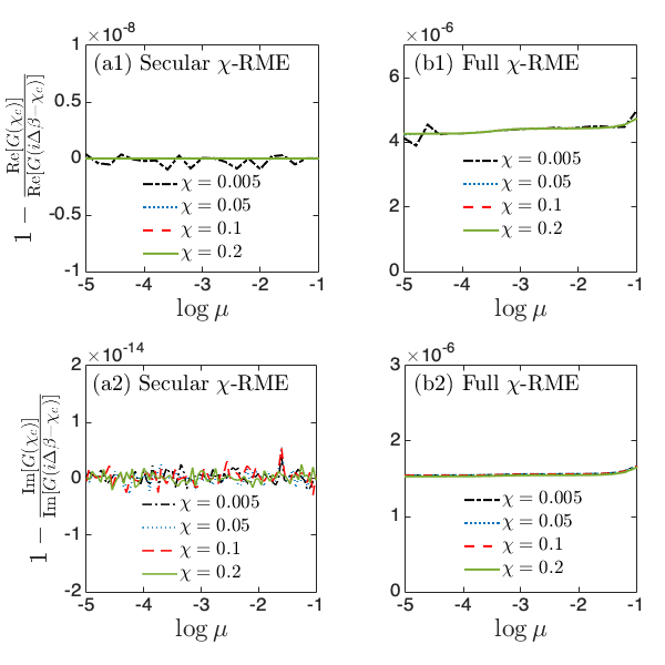
Figure 3: Analysis of the SSFS in the V-shaped system using the (a) secular and (b) full Redfield equation. We separately depict the real part of the CGF (top panels) and the imaginary part (bottom panels). Parameters are the same as in Fig. 1.

To address this issue we point out the following: (i) We are only interested in autonomous (non-driven) systems, and in their steady state properties. We are not aware of examples showing that the RME is thermodynamically improper in this case (unlike the transient regime). (ii) Across all parameters regimes that we had analyzed here, we found that levels population were positive (physical). (iii) The V-shaped model [see Eq. (22)] captures the behavior of coherences in the 4-level QAR, as discussed in Ref. Kilgour and Segal (2018). Below, we test the fluctuation symmetry in this (two-bath) model and show that it is obeyed with a small numerical error. While it is intriguing to prove that the $\chi$-RME satisfies the SSFS, our numerical simulations provide a strong support for this assertion, backing up our calculations of the current and its noise with Eq. (II.2). (v) We tested the entropy production rate in our simulations, and found that for results presented below it was always positive.

In fact, in all the tests that we carried out in this study, which were steady state calculations, we observed that the RME lead to positive level population, positive entropy production rate, and the validity of the SSFT. Our simulations provide a strong numerical support for the thermodynamical consistency of the RME in steady state, even when coherences play a critical role, calling for analytic investigations.

For simplicity, we now consider a model involving just two heat baths ($v=c,\leavevmode\nobreak\ h$). In steady state, the input heat at the terminal $v=h$ is equal to the heat output at $v=c$. As such, it is sufficient to look at the fluctuation symmetry of heat exchange with a single counting parameter. The exchange fluctuation symmetry states the following relation for the cumulant generating function Esposito et al. (2009); Campisi et al. (2011),

$$G(\chi_{c})\leavevmode\nobreak\ =\leavevmode\nobreak\ G(i\Delta\beta-\chi_{c}),$$ (21)

with $\Delta\beta=1/T_{h}-1/T_{c}$.

We simulate the V-shaped system coupled to two heat baths as an example, given that its behavior closely resembles that of Model I below [see Fig. 4 (a)] for the QAR Kilgour and Segal (2018). The system Hamiltonian involves a ground ($g$) state $|g\rangle$ and two excited ($e$) states $\{|e_{1}\rangle,|e_{2}\rangle\}$, which are coherently coupled,

$$\hat{H}_{s} = \epsilon_{g}|g\rangle\langle g|+\epsilon_{e}\Big{(}|e_{1}\rangle\langle e_{1}|+|e_{2}\rangle\langle e_{2}|\Big{)}$$ (22)

$$+\mu\Big{(}|e_{1}\rangle\langle e_{2}|+|e_{2}\rangle\langle e_{1}|\Big{)}.$$

Here $\epsilon_{g(e)}$ are the ground (excited) state energy. $\mu$ is the coupling strength between the two excited states and its magnitude can be made arbitrarily large. The transitions between ground and excited states are driven by the cold ($c$) and hot ($h$) heat baths with the following system operators associated with $\hat{H}_{sb}$:

$$\hat{S}_{h}\leavevmode\nobreak\ =\leavevmode\nobreak\ |g\rangle\langle e_{1}|+|e_{1}\rangle\langle g|,\leavevmode\nobreak\ \leavevmode\nobreak\ \hat{S}_{c}\leavevmode\nobreak\ =\leavevmode\nobreak\ |g\rangle\langle e_{2}|+|e_{2}\rangle\langle g|.$$ (23)

First, we verify Eq. (21) in the secular limit using Eq. (15) for which analytic treatments exist (see, for instance, Ref. Segal (2018)). In simulations, we determine the cumulant generating function by calculating numerically the eigenvalue with the smallest real part, Eq. (17). The dependence of $G(\chi_{c})$ and $G(\Delta\beta-\chi_{c})$ on the counting field $\chi_{c}$ and inter-state coupling strength $\mu$ is depicted in Fig. 1. By comparing the upper and lower panels of Fig. 1, it is evident that our simulations preserve the fluctuation symmetry Eq. (21) in the secular limit. Deviations between $G(\chi_{c})$ and $G(\Delta\beta-\chi_{c})$ were 11 orders of magnitude smaller than their value, for both real and imaginary parts (a quantitative analysis is included in Fig. 3). Since we know that the SSFS is obeyed in the secular limit, we reason that these deviations arise from numerical errors from the various stages involved in the procedure, such as matrix inversion. Particularly, we find that the real (imaginary) part of the cumulant generating function is an even (odd) function of the counting field $\chi_{c}$, hence Eq. (II.2) allows us to get real values for the current and its noise.

Next, we turn to simulations with the full $\chi$-RME Eq. (9). The comparison between $G(\chi_{c})$ and $G(i\Delta\beta-\chi_{c})$ is shown in Fig. 2. We observe that the fluctuation symmetry Eq. (21) is preserved by the full $\chi$-RME, thereby suggesting the thermodynamic consistency of the method for evaluating the currents and fluctuations from the cumulant generating function according to Eq. (II.2). Interestingly, we find that the magnitude of the cumulant generating function obtained using the full Redfield dynamics is suppressed in the weak coupling regime of $\mu$ compared with the secular limit, as illustrated in Fig. 1. We note that Ref. Kilgour and Segal (2018) demonstrated current suppression in the same model arising due to the presence of finite system coherence for weak $\mu$. Our results further imply that the so-observed suppression occurs at the level of cumulant generating function and persists for finite $\chi_{c}$.

We interrogate the SSFS in a quantitative way in Fig. 3 by looking at the deviation of the ratio $G(\chi_{c})/G(i\Delta\beta-\chi_{c})$ from unity, separately for the real and imaginary parts. The errors in the secular $\chi$-RME are certainly numerical since the SSFS is obeyed in this case. Turning to the full $\chi$-RME, we note higher deviations from unity for both real and imaginary parts compared to the secular case. However, deviations from perfect symmetry do not depend on the intersite coupling $\mu$ or the counting parameter $\chi$. Particularly for $\mu$, coherence effects show up in this model for $\log\mu\lesssim-3.5$ Kilgour and Segal (2018). The fact that the agreement between $G(\chi_{c})$ and $G(i\Delta\beta-\chi_{c})$ does not depend on $\mu$ suggests that the error is accumulated by numerical operations rather than reflecting a fundamental violation.

Note that the secular $\chi$-RME calculation on the V-shaped model is performed by studying the eigenvalue of a $3\times 3$ matrix. In contrast, the full $\chi$-RME calculation is performed by diagonalizing a $9\times 9$ matrix. As such, the computational effort, and thus error accumulation in these two cases is quite different.

To the best of our knowledge, simulations in Figs. 2-3 are the first strong numerical indication of the validity of the SSFS in the full Redfield formalism for multi-level systems, and for arbitrarily large $\chi$. We highlight that in fact we found that all eigenvalues of $\mathbb{L}_{\chi}$ obey the SSFS symmetry. Finally, predictions from the $\chi$-RME are obviously not exact given the perturbation approximation involved. In validating the SSFS for the $\chi$-RME we point out that though inaccurate, calculations of high order cumulants are physical (thermodynamically consistent).

III Quantum absorption refrigerators: Results

In Sec. II.3, we established the validity of the nonsecular $\chi$-RME, Eq. (9). Equipped with this method, we now study the steady-state behavior of QARs and contrast it to the secular limit, Eq. (15). We consider two distinct four-level QARs, with their level diagrams depicted in Fig. 4. To operate as a QAR, three heat baths, $v=h,c,w$ are included; the QAR continuously pumps heat from the cold ($c$) bath to the hot ($h$) bath consuming power from the work ($w$) bath.

Figure 4: Level schemes of the working medium of two quantum absorption refrigerators considered in this study. Transitions in green, red and blue are triggered by hot (H), work (W) and cold (C) heat baths, respectively. $g,\leavevmode\nobreak\ e$ and I denote the ground, excited and intermediate states in the local site basis, respectively. $\mu$ denotes the coupling strength between degenerate states (in the local basis). Model I was recently studied in Ref. Kilgour and Segal (2018). Model II with $\mu=0$ was investigated in Ref. Holubec and Novotný (2018).

We follow the standard setting, that QARs are composed of several subsystems that are spatially separated Mitchison (2019). This allows us to consider a selective coupling scheme, namely, each transition is triggered by an individual heat bath. With this prerequisite, Ref. Kilgour and Segal (2018) has shown that system coherences have deleterious effects on the cooling power of Model I [Fig. 4 (a)]. On the contrary, Ref. Holubec and Novotný (2018) found that system coherences can boost the cooling power of QARs in Model II [Fig. 4 (b)] with $\mu=0$. Nevertheless, both studies (cf. Refs. Kilgour and Segal (2018); Holubec and Novotný (2018)) were focused on the cooling power without examining its fluctuation behaviors. A recent study Holubec and Novotný (2019) had addressed the fluctuation behavior of Model II with $\mu=0$, that is, with an eigenenergy degeneracy. Close to maximum cooling current, this model displays a special behavior, with a non-unique steady state. Here, we consider the non-degenerate scenario with $\mu\neq 0$, which is very different, always resulting in a unique steady state solution.

Below, we perform a thorough investigation of Models I and II with a focus on the interplay of system coherences and power fluctuations. In what follows, we use the subscript ‘FR’ to denote results from the full $\chi$-RME Eq. (9) and ‘S’ for results from the secular $\chi$-RME Eq. (15).

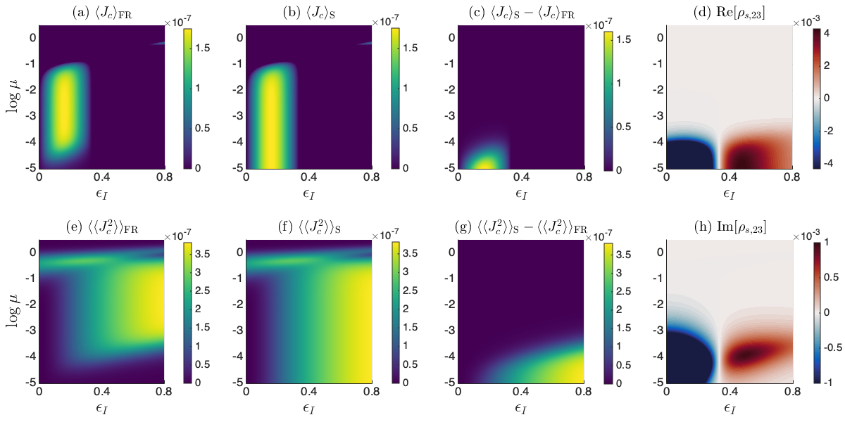
Figure 5: Current, noise and coherences in Model I. (a) Cooling power $\langle J_{c}\rangle_{\mathrm{FR}}$ obtained from the full $\chi$-RME [Eq. (9)]. (b) Cooling power $\langle J_{c}\rangle_{\mathrm{S}}$ obtained (b) from the secular $\chi$-RME [Eq. (15)]. The deep blue background in (a) and (b) marks the no-cooling region with $\langle J_{c}\rangle<0$ (not shown). (c) Power difference $\langle J_{c}\rangle_{\mathrm{S}}-\langle J_{c}\rangle_{\mathrm{FR}}$ in the cooling region. (e) Current fluctuations $\langle\langle J_{c}^{2}\rangle\rangle_{\mathrm{FR}}$ in the full $\chi$-RME [Eq. (9)]. (f) Current fluctuations $\langle\langle J_{c}^{2}\rangle\rangle_{\mathrm{S}}$ in the secular $\chi$-RME [Eq. (15)]. (g) Difference in fluctuations between the secular and non-secular calculations. (d) and (h) show the real (Re) and imaginary (Im) parts of the off-diagonal element of the reduced steady state density matrix, $\rho_{s,23}$, obtained from the full Redfield master equation. Parameters are $\alpha_{w,h,c}=0.002$, $\omega_{c}=50$, $T_{w}=0.2$, $T_{h}=0.15$, $T_{c}=0.1$, $\epsilon_{e}=1$.

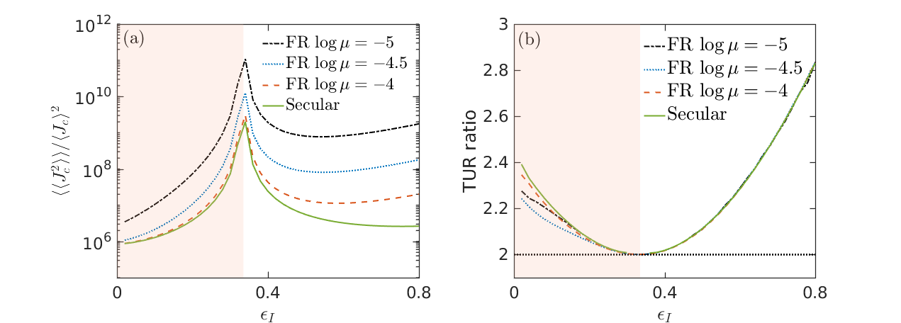
Figure 6: Relative noise and the TUR in Model I. (a) Relative noise $\langle\langle J_{c}^{2}\rangle\rangle/\langle J_{c}\rangle^{2}$ for different $\log\mu$. using the full $\chi$-RME [Eq. (9)]. The secular limit [Eq. (15)] does not depend on $\mu$. (b) Corresponding TUR ratio $\langle\langle J_{c}^{2}\rangle\rangle\langle\sigma\rangle/(\langle J_{c}\rangle^{2})$. The TUR bound (at two) is highlighted by a horizontal black dotted line. The shaded region marks the cooling region. Other parameters are the same with Fig. 5.

III.1 Model I

In the local site basis, the working medium of Model I (see Fig. 4 (a)) is described by a Hamiltonian

$$\hat{H}_{s}^{I} = \epsilon_{g}|g\rangle\langle g|+\epsilon_{e}|e\rangle\langle e|$$ (24)

$$+\epsilon_{I}(|\mathrm{I}_{1}\rangle\langle\mathrm{I}_{1}|+|\mathrm{I}_{2}\rangle\langle\mathrm{I}_{2}|)+\mu(|\mathrm{I}_{1}\rangle\langle\mathrm{I}_{2}|+|\mathrm{I}_{2}\rangle\langle\mathrm{I}_{1}|).$$

The system includes a ground (g) state $|g\rangle$, an excited (e) state $|e\rangle$, and two degenerate intermediate (I) levels ($|\mathrm{I}_{1}\rangle,\leavevmode\nobreak\ |\mathrm{I}_{2}\rangle$) connected by a coherent hoping rate $\mu$. Note that the levels are degenerate in the local basis, and non-degenerate in the global basis. We set the reference energy at $\epsilon_{g}=0$. The system’s operators involved in the system-bath interaction $\hat{H}_{sb}$ have the forms

$$\hat{S}_{c} = |g\rangle\langle\mathrm{I}_{2}|+|\mathrm{I}_{2}\rangle\langle g|,$$

$$\hat{S}_{h} = |g\rangle\langle e|+|e\rangle\langle g|,$$

$$\hat{S}_{w} = |\mathrm{I}_{1}\rangle\langle e|+|e\rangle\langle\mathrm{I}_{1}|.$$ (25)

After ordering the labels of eigenstates of $\hat{H}_{s}$ such that $\hat{H}_{s}=\sum_{i=1}^{4}E_{i}|i\rangle\langle i|$ with $E_{i}<E_{i+1}$, we rewrite the above system operators in the energy basis

$$\hat{S}_{c} = \frac{1}{\sqrt{2}}\left(|1\rangle\langle 3|-|1\rangle\langle 2|+\mathrm{H.c.}\right),$$

$$\hat{S}_{h} = |1\rangle\langle 4|+|4\rangle\langle 1|,$$

$$\hat{S}_{w} = \frac{1}{\sqrt{2}}\left(|2\rangle\langle 4|+|3\rangle\langle 4|+\mathrm{H.c.}\right).$$ (26)

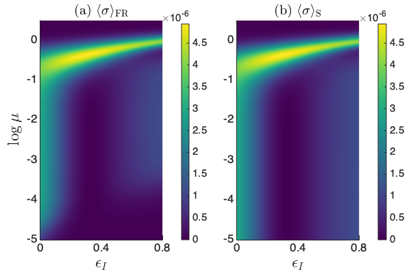
Figure 7: Verification of the positivity of the entropy production rate for Model I for the (a) full Redfield case, (b) secular limit. Parameters are the same as in Fig. 5.

In Fig. 5 we display simulation results for the current $\langle J_{c}\rangle$ (when referring to as cooling power we implicitly imply $\langle J_{c}\rangle>0$) and its noise $\langle\langle J_{c}^{2}\rangle\rangle$. From panels 5 (c) and (d) or (h) it is evident that finite system coherences, as quantified by the real or imaginary part of the steady state density matrix element $\rho_{s,23}$ is responsible for the suppression of the cooling power in the weak $\mu$ regime relative to the secular limit Kilgour and Segal (2018). Note that the deep blue background in panels (a) and (b) marks the no-cooling region, with $\langle J_{c}\rangle<0$. In other words, for presentation purposes we present the no-cooling region as zero cooling currents. The cooling region is marked in Fig. 6, where it appears when $\epsilon_{I}\lesssim 0.332$. Note that for the secular limit, results in all figures here and below were independent of $\mu$ for the small $\mu$ considered.

In Fig. 5 (e)-(f), we further show the current fluctuations. We find from panel 5 (e) and (f) that fluctuations become pronounced in the non-cooling region. Interestingly, the system coherence suppresses the current fluctuation but in the non-cooling region, as can be seen from the comparison between Fig. 5 (e) and (f). Noting that the signs of system coherence in the cooling and non-cooling regions are opposite [see Fig. 5 (d) and (h)], it is then clear that in Model I negative coherence in the cooling region induces power suppression, while positive coherence in the non-cooling region is responsible for the suppression of current fluctuations. Nevertheless, as we are interested in the cooling region, such a fluctuation suppression is of no practical use. Intriguingly, the marginal regions between finite coherences in Fig. 5 (d) and (h) marks the boundary of cooling and non-cooling regions, namely, the transition from cooling to non-cooling regions is associated with a sign change of system coherence.

We now look at the relative noise, $\langle\langle J_{c}^{2}\rangle\rangle/\langle J_{c}\rangle^{2}$ and the TUR ratio $\langle\langle J_{c}^{2}\rangle\rangle\langle\sigma\rangle/\langle J_{c}\rangle^{2}$, see Fig. 6. In panel 6 (a) we observe that the relative noise obtained from the full $\chi$-QME is greatly enhanced due to the presence of coherences in both the cooling and non-cooling regions, compared to the secular limit. Ideally, the relative noise tends to infinity at the exact boundary of cooling and non-cooling regions as $\langle J_{c}\rangle=0$, however, we can only see finite peak structures centered around the boundary from panel 6 (a) since we utilize discretized values for $\epsilon_{I}$ in simulations and may not be able to reach the exact boundary.

The TUR ratio is plotted in panel 6 (b). We observe that: (i) The TUR ratio is always above the classical bound set by the TUR Eq. (19). (ii) The TUR ratio saturates to the bound at the point when the entropy production is exactly zero and the refrigerator crosses into the no-cooling region. (iii) Coherences slightly reduce the TUR ratio, relative to the secular limit, yet the behavior is non-monotonic. Nevertheless, coherences only mildly reduce the TUR ratio from the secular limit. The calculation of the TUR ratio at the cooling-no-cooling boundary region is nontrivial numerically. This is due to the nontrivial cancellation between entropy production and the relative noise taking place when approaching the boundary. As such, very close to the boundary region the TUR ratio was not evaluated.

Back to the fundamental question as to whether the non-secular Redfield equation is suitable (thermodynamically consistent) for studying current noise. In Fig. 7 we verify that the entropy production rate is always positive with our parameters. In fact, we have not observed negative entropy production rates in any of our simulations. As such, we hypothesize that the Redfield equation is thermodynamically consistent in the steady state limit with $\langle\sigma\rangle>0$, beyond our case study. This result does not exclude the possibility of observing fundamental deficiencies with the Redfield equation in the transient regime.

Concluding this Section: The TUR, Eq. (19), is satisfied by Model I in the presence of system coherences. Notably, the TUR ratio of Model I is almost independent of the inter-site coupling strength $\mu$, and it almost coincides with that of the secular limit, thereby implying that the coherence-induced enhancement of the relative noise is compensated by the coherence-induced reduction of entropy production rate, which is proportional to the heat currents.

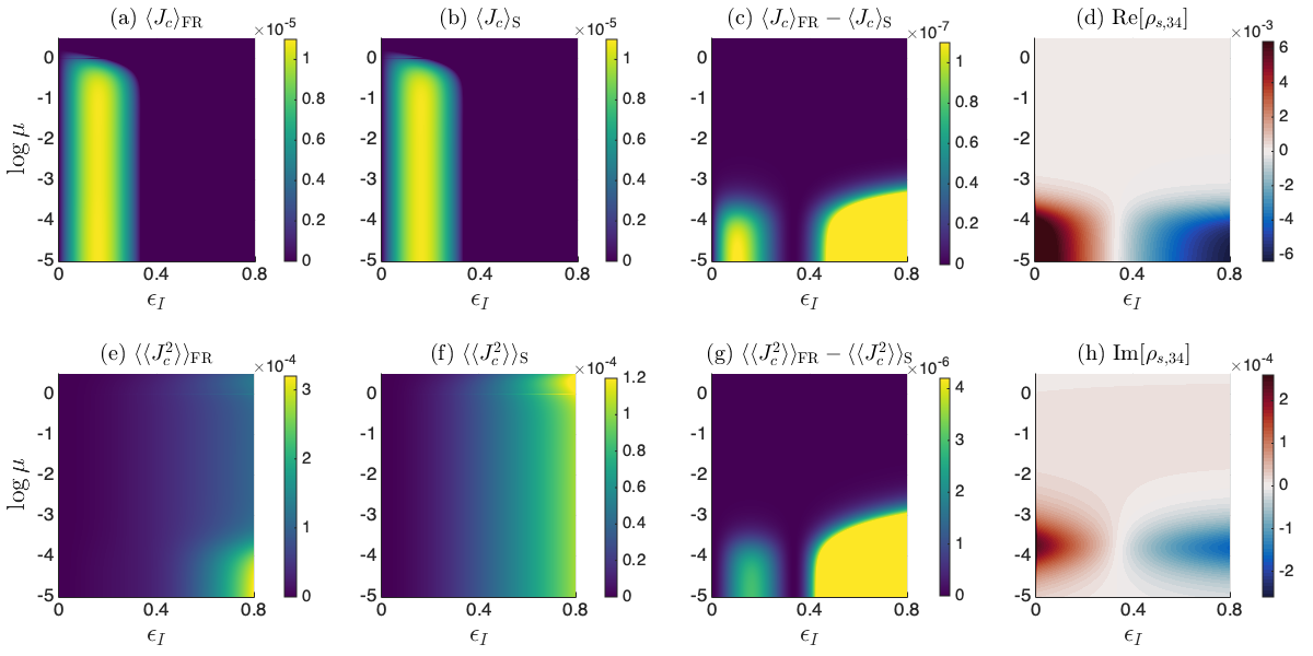
Figure 8: Current, fluctuations and coherence in Model II. (a) Cooling power $\langle J_{c}\rangle_{\mathrm{FR}}$ obtained from the full $\chi$-RME [Eq. (9)]. (b) Cooling power $\langle J_{c}\rangle_{\mathrm{S}}$ from the secular $\chi$-RME [Eq. (15)]. The deep blue backgrounds in (a) and (b) mark the no-cooling region with $\langle J_{c}\rangle<0$ (not shown). (c) The difference in the cooling current, $\langle J_{c}\rangle_{\mathrm{FR}}-\langle J_{c}\rangle_{\mathrm{S}}$ in the whole region. (e) Current fluctuations $\langle\langle J_{c}^{2}\rangle\rangle_{\mathrm{FR}}$ from the full $\chi$-RME [Eq. (9)]. (f) Current fluctuations $\langle\langle J_{c}^{2}\rangle\rangle_{\mathrm{S}}$ in the secular $\chi$-RME [Eq. (15)]. (g) The difference $\langle\langle J_{c}^{2}\rangle\rangle_{\mathrm{FR}}-\langle\langle J_{c}^{2}\rangle\rangle_{\mathrm{S}}$ in the whole region. (d) and (h) show the real (Re) and imaginary (Im) parts of the off-diagonal element of the reduced steady state density matrix, $\rho_{s,34}$, obtained from the full Redfield master equation. Parameters are $\alpha_{c}=0.002$, $\alpha_{h1}=0.8\alpha_{c}$, $\alpha_{h2}=\alpha_{c}$, $\alpha_{w1}=\alpha_{c}$, $\alpha_{w2}=\alpha_{c}$, $\omega_{c}=50$, $T_{w}=2$, $T_{h}=0.6$, $T_{c}=0.25$, $\epsilon_{e}=1$.

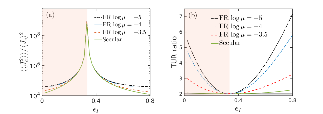
Figure 9: Relative noise and the TUR in Model II. (a) Relative noise $\langle\langle J_{c}^{2}\rangle\rangle/\langle J_{c}\rangle^{2}$ for different $\log\mu$. using the full $\chi$-RME [Eq. (9)]. The secular limit [Eq. (15)] does not depend on $\mu$. (b) Corresponding TUR ratio $\langle\langle J_{c}^{2}\rangle\rangle\langle\sigma\rangle/(\langle J_{c}\rangle^{2})$. The TUR bound (at two) is highlighted by a horizontal black dotted line. The shaded region marks the cooling region. Other parameters are the same with Fig. 8.

III.2 Model II

We turn to Model II for a QAR, as illustrated in Fig. 4 (b). Previously, Refs. Holubec and Novotný (2018, 2019) demonstrated that this model can have a coherence-induced enhancement of the cooling power; below we confirm this scenario and further show in the Appendix that this model also permits an adverse effect of system coherence on the cooling power, when varying the system-bath coupling strengths.

The working medium of Model II is described by a four level Hamiltonian in the local basis

$$\hat{H}_{s}^{II} = \epsilon_{e}(|e_{1}\rangle\langle e_{1}|+|e_{2}\rangle\langle e_{2}|)+\mu(|e_{1}\rangle\langle e_{2}|+|e_{2}\rangle\langle e_{1}|)$$ (27)

$$+\epsilon_{g}|g\rangle\langle g|+\epsilon_{I}|\mathrm{I}\rangle\langle\mathrm{I}|.$$

The system involves a ground (g) state $|g\rangle$, an intermediate (I) state $|\mathrm{I}\rangle$ and two degenerate excited (e) states ($|e_{1}\rangle,\leavevmode\nobreak\ |e_{2}\rangle$) that are connected by a coherent hoping rate, $\mu$. We set the reference energy at $\epsilon_{g}=0$. After ordering the labels of eigenstates of $\hat{H}_{s}$ such that $\hat{H}_{s}=\sum_{i=1}^{4}E_{i}|i\rangle\langle i|$ with $E_{i}<E_{i+1}$, we get the following system operators, involved in the system-bath interaction $\hat{H}_{sb}$, in the energy basis Holubec and Novotný (2018)

$$\hat{S}_{c} = |1\rangle\langle 2|+|2\rangle\langle 1|,$$

$$\hat{S}_{h} = \sqrt{\alpha_{h2}}|1\rangle\langle 4|+\sqrt{\alpha_{h1}}|1\rangle\langle 3|+\mathrm{H.c.},$$

$$\hat{S}_{w} = \sqrt{\alpha_{w2}}|2\rangle\langle 4|+\sqrt{\alpha_{w1}}|2\rangle\langle 3|+\mathrm{H.c.}.$$ (28)

The real-valued parameters $\alpha_{vk}$ are dimensionless; they are taken from the spectral density function $\gamma_{v}(\omega)$ in Eq. (14); recall that we model the spectral density function as $\gamma_{v}=\alpha_{v}\omega e^{-\omega/\omega_{c}}$. Here for convenience we absorbed $\alpha_{vk}$ into the definitions of $\hat{S}_{h,w}$ so as to allow scenarios where different transitions induced by the same bath are enhanced by different coupling strengths.

Fig. 8 depicts an example where system coherences boost the cooling power, as predicted in Refs. Holubec and Novotný (2018, 2019). This is highlighted in panel 8 (c), where we show the current difference $\langle J_{c}\rangle_{\mathrm{FR}}-\langle J_{c}\rangle_{\mathrm{S}}$ in both the cooling and no-cooling regions. As can be seen, the cooling power $\langle J_{c}\rangle_{\mathrm{FR}}$ in the cooling region is slightly enhanced compared with $\langle J_{c}\rangle_{\mathrm{S}}$ when $\mu$ is relatively small. We attribute this cooling power enhancement to the finite positive system coherence in that region as indicated in Fig. 8 (d) and (h). However, panel 8 (g) shows that this cooling power enhancement comes at the price of an enhanced power fluctuation. Similarly to Model I, here we also find that the marginal region between nonzero coherences (Fig. 8 (d) and (h)) marks the boundary between the cooling and the no-cooling regions.

While in Fig. 8 system coherences enhance the cooling current, in the Appendix we show the opposite effect within the same model, but using a different value for $\alpha_{h1}$. This coherence-induced suppression of the cooling power (similarly to Model I) becomes evident by combining the information of Fig. A1 (c) and (d) or (h).

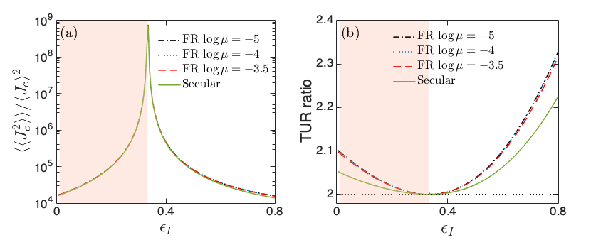
Figure A2: Relative noise and the TUR in Model II with $\alpha_{h1}=0.1\alpha_{c}$; other parameters are the same with Fig. 8. (a) Relative noise $\langle\langle J_{c}^{2}\rangle\rangle/\langle J_{c}\rangle^{2}$ for different $\log\mu$. using the full $\chi$-RME [Eq. (9)]. The secular limit [Eq. (15)] does not depend on $\mu$. (b) Corresponding TUR ratio $\langle\langle J_{c}^{2}\rangle\rangle\langle\sigma\rangle/(\langle J_{c}\rangle^{2})$. The TUR bound (at two) is highlighted by a horizontal black dotted line. The shaded region marks the cooling region.

Even though system coherences can either suppress or enhance the cooling power in Model II (depending on the system-bath coupling strengths), in Fig. 9 (a) we again observe that the relative noise obtained from the full $\chi$-RME is larger than that obtained from the secular $\chi$-RME. Furthermore, the relative noise approaches the secular limit near the boundary between the cooling and no-cooling regions. Nevertheless, from Fig. 9 (b) (together with Fig. A2 (b) in the Appendix) we find that the TUR holds as well in Model II. Interestingly, the TUR ratio is enhanced by coherences relative to the secular limit: In Fig. 9 (b), we see that the TUR ratio in the secular case is very close to the bound within the whole range of $\epsilon_{I}$, while it is factor of 3 greater in the coherent case.

Overall, we found that in model II the effect of coherences on the cooling current was very mild; we did not perform detailed simulations to identify region of more substantial cooling effect as this was not the objective of this work. Our main conclusion, which holds for all cases examined here is that while coherences may boost or suppress the cooling current, their effect on fluctuations is adverse, thus validating the standard TUR.

IV Summary

In summary, we addressed the interplay of system coherences and fluctuations of the cooling current in the performance of steady-state QARs. Using a Redfield master equation with a full counting statistics information, we obtained the behaviors of the cooling power and its fluctuations, for steady-state QAR models with (or without) system coherences. Remarkably, we found that the relative noise of the cooling power was always enhanced in the presence of system coherence, even though the cooling power itself was either suppressed or enhanced, depending on the model and its parameters. As a result, we confirmed that the TUR derived for classical Markov-jump processes holds for steady-state QARs in the presence of system coherence; the performance of the steady-state QARs is still constrained by the classical tradeoff relation.

Our results apply to scenarios where the Redfield master equation can be justified. Although a general proof within the framework of the Redfield master equation is still missing, we expect that our results are general: System coherence corroborates the classical TUR. After all, system coherences correspond to additional quantum fluctuations, on top of thermal ones to the QTMs. In fact, a recent study on steady-state quantum heat engines Rignon-Bret et al. (2020) reached a similar conclusion on the role of system coherences in validating the TUR. However, if cyclic instead of steady-state QTMs are concerned, our conclusions need to be revisited as a recent study Cangemi et al. (2020) suggested that system coherences can help to violate a TUR specific for periodic-driven systems.

Is there a “quantum” advantage for thermal machines, compared to their classical counterparts? While the power output may be enhanced due to coherences—depending on the model employed, here we point out to what seems to be a more general adverse effect of quantum coherences: According to our examples, QTMs suffer more pronounced thermodynamic fluctuations arising due to finite system coherence, compared to the incoherent analogue. Our findings further imply that fluctuations should be considered when assessing whether the system coherence is a useful resource to the operation of QTMs.

Altogether, our contributions are: (i) We verified with simulations that the counting-field dressed Redfield master equation satisfies the SSFS for heat transfer. (ii) We demonstrated that system coherences intensify relative current fluctuations, irrespective of the impact on the cooling power. (iii) We showed that the classical TUR holds in the presence of system coherences.

As a final remark, our study indicates that the standard (classical) TUR for steady state transport is valid in the weak system-bath coupling regime (see also Ref. Saryal et al. (2019)). To observe violations—thus circumvent the classical tradeoff relation for thermal machines—one should turn to the nonperturbative system-bath coupling regime Agarwalla and Segal (2017), where system-bath entanglement and nonmarkovianity play a decisive role in breaking the TUR Saryal et al. (2019).

Appendix A Additional simulations for Model II

In this appendix, we show that Model II can also allow for a coherence-induced suppression of the cooling power when varying the system-bath coupling strength, say, $\alpha_{h1}$. A representative set of results with $\alpha_{h1}=0.1\alpha_{c}$ is depicted in Figs. A1 and A2. The cooling power suppression becomes evident by inspecting Fig. A1 (c) and (d) or (h).

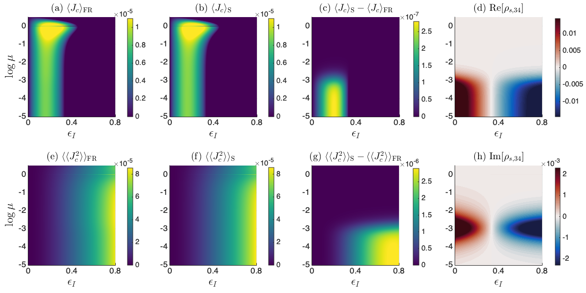
Figure A1: Current, fluctuations and coherence in Model II with $\alpha_{h1}=0.1\alpha_{c}$; other parameters are the same as in Fig. 8. (a) Cooling power $\langle J_{c}\rangle_{\mathrm{FR}}$ obtained from the full $\chi$-RME [Eq. (9)]. (b) Cooling power $\langle J_{c}\rangle_{\mathrm{S}}$ from the secular $\chi$-RME [Eq. (15)]. The deep blue backgrounds in (a) and (b) mark the no-cooling region with $\langle J_{c}\rangle<0$ (not shown). (c) Difference in cooling current $\langle J_{c}\rangle_{\mathrm{S}}-\langle J_{c}\rangle_{\mathrm{FR}}$ in the whole region. (e) Current fluctuations $\langle\langle J_{c}^{2}\rangle\rangle_{\mathrm{FR}}$ from the full $\chi$-RME [Eq. (9)]. (f) Current fluctuations $\langle\langle J_{c}^{2}\rangle\rangle_{\mathrm{S}}$ in the secular $\chi$-RME [Eq. (15)]. (g) The difference $\langle\langle J_{c}^{2}\rangle\rangle_{\mathrm{S}}-\langle\langle J_{c}^{2}\rangle\rangle_{\mathrm{FR}}$ in the whole region. (d) and (h) show the real (Re) and imaginary (Im) parts of the off-diagonal element of the reduced steady state density matrix, $\rho_{s,34}$, obtained from the full Redfield master equation.

References

- Scovil and Schulz-DuBois (1959) H. E. D. Scovil and E. O. Schulz-DuBois, “Three-level masers as heat engines,” Phys. Rev. Lett. 2, 262 (1959).
- Geva and Kosloff (1992a) E. Geva and R. Kosloff, “On the classical limit of quantum thermodynamics in finite time,” J. Chem. Phys. 97, 4398 (1992a).
- Gemmer et al. (2009) J. Gemmer, M. Michel, and G. Mahler, Quantum Thermodynamics (Springer-Verlag, Berlin, 2009).
- Seifert (2012) U. Seifert, “Stochastic thermodynamics, fluctuation theorems and molecular machines,” Rep. Prog. Phys. 75, 126001 (2012).
- Pekola (2015) J. P. Pekola, “Towards quantum thermodynamics in electronic circuits,” Nat. Phys. 11, 118 (2015).
- Kosloff (2013) R. Kosloff, “Quantum thermodynamics: A dynamical viewpoint,” Entropy 15, 2100 (2013).
- Goold et al. (2016) J. Goold, M. Huber, A. Riera, L. del Rio, and P. Skrzypczyk, “The role of quantum information in thermodynamics?a topical review,” J. Phys. A: Math. Theor. 49, 143001 (2016).
- Vinjanampathy and Anders (2016) S. Vinjanampathy and J. Anders, “Quantum thermodynamics,” Contemp. Phys. 57, 545 (2016).
- Binder et al. (2018) F. Binder, L. A. Correa, C. Gogolin, J. Anders, and G. Adesso, Thermodynamics in the Quantum Regime (Springer International, 2018).
- Seifert (2019) U. Seifert, “From stochastic thermodynamics to thermodynamic inference,” Annu. Rev. Condens. Matter Phys. 10, 171 (2019).
- Pekola and Khaymovich (2019) J. P. Pekola and I. M. Khaymovich, “Thermodynamics in single-electron circuits and superconducting qubits,” Annu. Rev. Condens. Matter Phys. 10, 193 (2019).
- Talkner et al. (2007) P. Talkner, E. Lutz, and P. Hänggi, “Fluctuation theorems: Work is not an observable,” Phys. Rev. E 75, 050102 (2007).
- Talkner and Hänggi (2016) P. Talkner and P. Hänggi, “Aspects of quantum work,” Phys. Rev. E 93, 022131 (2016).
- Talkner and Hänggi (2020) P. Talkner and P. Hänggi, “Colloquium: Statistical mechanics and thermodynamics at strong coupling: Quantum and classical,” Rev. Mod. Phys. 92, 041002 (2020).
- Esposito et al. (2009) M. Esposito, U. Harbola, and S. Mukamel, “Nonequilibrium fluctuations, fluctuation theorems, and counting statistics in quantum systems,” Rev. Mod. Phys. 81, 1665–1702 (2009).
- Campisi et al. (2011) M. Campisi, P. Hänggi, and P. Talkner, “Colloquium: Quantum fluctuation relations: Foundations and applications,” Rev. Mod. Phys. 83, 771–791 (2011).
- Alicki (1979) R Alicki, “The quantum open system as a model of the heat engine,” J. Phys. A: Math. Gen. 12, L103 (1979).
- Geva and Kosloff (1992b) E. Geva and R. Kosloff, “A quantum?mechanical heat engine operating in finite time. a model consisting of spin?1/2 systems as the working fluid,” J. Chem. Phys. 96, 3054 (1992b).
- Giazotto et al. (2006) F. Giazotto, T. T. Heikkilä, A. Luukanen, A. M. Savin, and J. P. Pekola, “Opportunities for mesoscopics in thermometry and refrigeration: Physics and applications,” Rev. Mod. Phys. 78, 217–274 (2006).
- Filliger and Reimann (2007) R. Filliger and P. Reimann, “Brownian gyrator: A minimal heat engine on the nanoscale,” Phys. Rev. Lett. 99, 230602 (2007).
- Esposito et al. (2010) M. Esposito, R. Kawai, K. Lindenberg, and C. Van den Broeck, “Efficiency at maximum power of low-dissipation carnot engines,” Phys. Rev. Lett. 105, 150603 (2010).
- Linden et al. (2010) N. Linden, S. Popescu, and P. Skrzypczyk, “How small can thermal machines be? the smallest possible refrigerator,” Phys. Rev. Lett. 105, 130401 (2010).
- Levy and Kosloff (2012) A. Levy and R. Kosloff, “Quantum absorption refrigerator,” Phys. Rev. Lett. 108, 070604 (2012).
- Abah et al. (2012) O. Abah, J. Roßnagel, G. Jacob, S. Deffner, F. Schmidt-Kaler, K. Singer, and E. Lutz, “Single-ion heat engine at maximum power,” Phys. Rev. Lett. 109, 203006 (2012).
- Blickle and Bechinger (2012) V. Blickle and C. Bechinger, “Realization of a micrometre-sized stochastic heat engine,” Nat. Phys. 8, 143–146 (2012).
- Kosloff and Levy (2014) R. Kosloff and A. Levy, “Quantum heat engines and refrigerators: Continuous devices,” Ann. Rev. Phys. Chem. 65, 365–393 (2014).
- Roßnagel et al. (2014) J. Roßnagel, O. Abah, F. Schmidt-Kaler, K. Singer, and E. Lutz, “Nanoscale heat engine beyond the carnot limit,” Phys. Rev. Lett. 112, 030602 (2014).
- Thierschmann et al. (2015) H. Thierschmann, R. S nchez, B. Sothmann, F. Arnold, C. Heyn, W. Hansen, H. Buhmann, and L. W. Molenkamp, “Three-terminal energy harvester with coupled quantum dots,” Nat. Nanotechnol. 10, 854 (2015).
- Dechant et al. (2015) A. Dechant, N. Kiesel, and E. Lutz, “All-optical nanomechanical heat engine,” Phys. Rev. Lett. 114, 183602 (2015).
- Harris (2016) S. E. Harris, “Electromagnetically induced transparency and quantum heat engines,” Phys. Rev. A 94, 053859 (2016).
- Robnagel et al. (2016) J. Robnagel, S. T. Dawkins, K. N. Tolazzi, O. Abah, E. Lutz, F. Schmidt-Kaler, and K. Singer, “A single-atom heat engine,” Science 352, 325 (2016).
- Uzdin et al. (2015) R. Uzdin, A. Levy, and R. Kosloff, “Equivalence of quantum heat machines, and quantum-thermodynamic signatures,” Phys. Rev. X 5, 031044 (2015).
- Hofer et al. (2016a) P. P. Hofer, J.-R. Souquet, and A. A. Clerk, “Quantum heat engine based on photon-assisted cooper pair tunneling,” Phys. Rev. B 93, 041418 (2016a).
- Hofer et al. (2016b) P. P. Hofer, M. Perarnau-Llobet, J. Brask, R. Silva, M. Huber, and N. Brunner, “Autonomous quantum refrigerator in a circuit qed architecture based on a josephson junction,” Phys. Rev. B 94, 235420 (2016b).
- Zou et al. (2017) Y. Zou, Y. Jiang, Y. Mei, X. Guo, and S. Du, “Quantum heat engine using electromagnetically induced transparency,” Phys. Rev. Lett. 119, 050602 (2017).
- Martinez et al. (2016) I. A. Martinez, E. Roldan, L. Dinis, D. Petrov, J. M. R. Parrondo, and R. A. Rica, “Brownian carnot engine,” Nat. Phys. 12, 67–70 (2016).
- Ghosh et al. (2017) A. Ghosh, C. L. Latune, L. Davidovich, and G. Kurizki, “Catalysis of heat-to-work conversion in quantum machines,” Proc. Natl. Acad. Sci. U.S.A. 114, 12156 (2017).
- Klaers et al. (2017) J. Klaers, S. Faelt, A. Imamoglu, and E. Togan, “Squeezed thermal reservoirs as a resource for a nanomechanical engine beyond the carnot limit,” Phys. Rev. X 7, 031044 (2017).
- Elouard et al. (2017) C. Elouard, D. Herrera-Martí, B. Huard, and A. Auffèves, “Extracting work from quantum measurement in maxwell’s demon engines,” Phys. Rev. Lett. 118, 260603 (2017).
- Abah and Lutz (2017) O. Abah and E. Lutz, “Energy efficient quantum machines,” Europhys. Lett. 118, 40005 (2017).
- Benenti et al. (2017) G. Benenti, G. Casati, K. Saito, and R. S. Whitney, “Fundamental aspects of steady-state conversion of heat to work at the nanoscale,” Phys. Rep. 694, 1 (2017), fundamental aspects of steady-state conversion of heat to work at the nanoscale.
- Ronzani et al. (2018) A. Ronzani, B. Karimi, J. Senior, Y. Chang, J. T. Peltonen, C. Chen, and J. P. Pekola, “Tunable photonic heat transport in a quantum heat valve,” Nat. Phys. 14, 991 (2018).
- Josefsson et al. (2018) M. Josefsson, A. Svilans, A. M. Burke, E. A. Hoffmann, S. Fahlvik, C. Thelander, M. Leijnse, and H. Linke, “A quantum-dot heat engine operating close to the thermodynamic efficiency limits,” Nat. Nanotechnol. 13, 920 (2018).
- Friedman et al. (2018) H. Friedman, B. Agarwalla, and D. Segal, “Quantum energy exchange and refrigeration: a full-counting statistics approach,” New J. Phys. 20, 083026 (2018).
- Kilgour and Segal (2018) M. Kilgour and D. Segal, “Coherence and decoherence in quantum absorption refrigerators,” Phys. Rev. E 98, 012117 (2018).
- Elouard and Jordan (2018) C. Elouard and A. N. Jordan, “Efficient quantum measurement engines,” Phys. Rev. Lett. 120, 260601 (2018).
- Pietzonka et al. (2019) P. Pietzonka, É. Fodor, C. Lohrmann, M. E. Cates, and U. Seifert, “Autonomous engines driven by active matter: Energetics and design principles,” Phys. Rev. X 9, 041032 (2019).
- de Assis et al. (2019) R. J. de Assis, T. M. de Mendonca, C. J. Villas-Boas, A. M. de Souza, R. S. Sarthour, I. S. Oliveira, and N. G. de Almeida, “Efficiency of a quantum otto heat engine operating under a reservoir at effective negative temperatures,” Phys. Rev. Lett. 122, 240602 (2019).
- Mitchison (2019) M. T. Mitchison, “Quantum thermal absorption machines: refrigerators, engines and clocks,” Contemp. Phys. 60, 164 (2019).
- Peterson et al. (2019) J. P. S. Peterson, T. B. Batalhão, M. Herrera, A. M. Souza, R. S. Sarthour, I. S. Oliveira, and R. M. Serra, “Experimental characterization of a spin quantum heat engine,” Phys. Rev. Lett. 123, 240601 (2019).
- Klatzow et al. (2019) J. Klatzow, J. N. Becker, P. M. Ledingham, C. Weinzetl, K. T. Kaczmarek, D. J. Saunders, J. Nunn, I. A. Walmsley, R. Uzdin, and E. Poem, “Experimental demonstration of quantum effects in the operation of microscopic heat engines,” Phys. Rev. Lett. 122, 110601 (2019).
- von Lindenfels et al. (2019) D. von Lindenfels, O. Gräb, C. T. Schmiegelow, V. Kaushal, J. Schulz, M. T. Mitchison, J. Goold, F. Schmidt-Kaler, and U. G. Poschinger, “Spin heat engine coupled to a harmonic-oscillator flywheel,” Phys. Rev. Lett. 123, 080602 (2019).
- Buffoni et al. (2019) L. Buffoni, A. Solfanelli, P. Verrucchi, A. Cuccoli, and M. Campisi, “Quantum measurement cooling,” Phys. Rev. Lett. 122, 070603 (2019).
- Abiuso and Perarnau-Llobet (2020) P. Abiuso and M. Perarnau-Llobet, “Optimal cycles for low-dissipation heat engines,” Phys. Rev. Lett. 124, 110606 (2020).
- Carollo et al. (2020) F. Carollo, F. M. Gambetta, K. Brandner, J. P. Garrahan, and I. Lesanovsky, “Nonequilibrium quantum many-body rydberg atom engine,” Phys. Rev. Lett. 124, 170602 (2020).
- Hartmann et al. (2020) A. Hartmann, V. Mukherjee, W. Niedenzu, and W. Lechner, “Many-body quantum heat engines with shortcuts to adiabaticity,” Phys. Rev. Research 2, 023145 (2020).
- Van Horne et al. (2020) N. Van Horne, D. Yum, T. Dutta, P. Hänggi, J. Gong, D. Poletti, and M. Mukherjee, “Single-atom energy-conversion device with a quantum load,” npj Quantum Inf. 6, 37– (2020).
- Ono et al. (2020) K. Ono, S. N. Shevchenko, T. Mori, S. Moriyama, and Franco Nori, “Analog of a quantum heat engine using a single-spin qubit,” Phys. Rev. Lett. 125, 166802 (2020).
- Bhandari et al. (2020) B. Bhandari, P. Alonso, F. Taddei, F. von Oppen, R. Fazio, and L. Arrachea, “Geometric properties of adiabatic quantum thermal machines,” Phys. Rev. B 102, 155407 (2020).
- Scully et al. (2003) M. O. Scully, M. S. Zubairy, G. S. Agarwal, and H. Walther, “Extracting work from a single heat bath via vanishing quantum coherence,” Science 299, 862 (2003).
- Zhang et al. (2007) T. Zhang, W. Liu, P. Chen, and C. Li, “Four-level entangled quantum heat engines,” Phys. Rev. A 75, 062102 (2007).
- Dillenschneider and Lutz (2009) R. Dillenschneider and E. Lutz, “Energetics of quantum correlations,” Europhys. Lett. 88, 50003 (2009).
- Scully et al. (2011) M. O. Scully, K. R. Chapin, K. E. Dorfman, M. Kim, and A. Svidzinsky, “Quantum heat engine power can be increased by noise-induced coherence,” Proc. Natl. Acad. Sci. U.S.A. 108, 15097 (2011).
- Dorfman et al. (2013) K. E. Dorfman, D. V. Voronine, S. Mukamel, and M. O. Scully, “Photosynthetic reaction center as a quantum heat engine,” Proc. Natl. Acad. Sci. U.S.A. 110, 2746 (2013).
- Rahav et al. (2012) S. Rahav, U. Harbola, and S. Mukamel, “Heat fluctuations and coherences in a quantum heat engine,” Phys. Rev. A 86, 043843 (2012).
- Killoran et al. (2015) N. Killoran, S. F. Huelga, and M. B. Plenio, “Enhancing light-harvesting power with coherent vibrational interactions: A quantum heat engine picture,” J. Chem. Phys. 143, 155102 (2015).
- Leggio et al. (2015) B. Leggio, B. Bellomo, and M. Antezza, “Quantum thermal machines with single nonequilibrium environments,” Phys. Rev. A 91, 012117 (2015).
- Niedenzu et al. (2015) W. Niedenzu, D. Gelbwaser-Klimovsky, and G. Kurizki, “Performance limits of multilevel and multipartite quantum heat machines,” Phys. Rev. E 92, 042123 (2015).
- Gelbwaser-Klimovsky et al. (2015) D. Gelbwaser-Klimovsky, W. Niedenzu, P. Brumer, and G. Kurizki, “Power enhancement of heat engines via correlated thermalization in a three-level ?working fluid?,” Sci. Rep. 5, 14413 (2015).
- Brandner et al. (2015) K. Brandner, M. Bauer, M. T Schmid, and U. Seifert, “Coherence-enhanced efficiency of feedback-driven quantum engines,” New J. Phys. 17, 065006 (2015).
- Mitchison et al. (2015) M. T Mitchison, M. P Woods, J. Prior, and M. Huber, “Coherence-assisted single-shot cooling by quantum absorption refrigerators,” New J. Phys. 17, 115013 (2015).
- Su et al. (2016) S. Su, C. Sun, S. Li, and J. Chen, “Photoelectric converters with quantum coherence,” Phys. Rev. E 93, 052103 (2016).
- Türkpençe and Müstecaplıoğlu (2016) D. Türkpençe and Ö. E. Müstecaplıoğlu, “Quantum fuel with multilevel atomic coherence for ultrahigh specific work in a photonic carnot engine,” Phys. Rev. E 93, 012145 (2016).
- Uzdin (2016) R. Uzdin, “Coherence-induced reversibility and collective operation of quantum heat machines via coherence recycling,” Phys. Rev. Applied 6, 024004 (2016).
- Mehta and Johal (2017) V. Mehta and R. S. Johal, “Quantum otto engine with exchange coupling in the presence of level degeneracy,” Phys. Rev. E 96, 032110 (2017).
- Chen et al. (2017) F. Chen, Y. Gao, and M. Galperin, “Molecular heat engines: Quantum coherence effects,” Entropy 19, 472 (2017).
- Holubec and Novotný (2018) V. Holubec and T. Novotný, “Effects of noise-induced coherence on the performance of quantum absorption refrigerators,” J. Low Temp. Phys. 192, 147–168 (2018).
- Wertnik et al. (2018) M. Wertnik, A. Chin, F. Nori, and N. Lambert, “Optimizing co-operative multi-environment dynamics in a dark-state-enhanced photosynthetic heat engine,” J. Chem. Phys. 149, 084112 (2018).
- Holubec and Novotný (2019) V. Holubec and T. Novotný, “Effects of noise-induced coherence on the fluctuations of current in quantum absorption refrigerators,” J. Chem. Phys. 151, 044108 (2019).
- Latune et al. (2019) C. L. Latune, I. Sinayskiy, and F. Petruccione, “Quantum coherence, many-body correlations, and non-thermal effects for autonomous thermal machines,” Sci. Rep. 9, 3191 (2019).
- Latune et al. (2020) C. L. Latune, I. Sinayskiy, and F. Petruccione, “Roles of quantum coherences in thermal machines,” (2020), arXiv:2006.01166.
- Francica et al. (2020) G. Francica, F. C. Binder, G. Guarnieri, M. T. Mitchison, J. Goold, and F. Plastina, “Quantum coherence and ergotropy,” Phys. Rev. Lett. 125, 180603 (2020).
- Verley et al. (2014) G. Verley, M. Esposito, T. Willaert, and C. Van den Broeck, “The unlikely carnot efficiency,” Nat. Commun. 5, 4721 (2014).
- Esposito et al. (2015) M. Esposito, M. A. Ochoa, and M. Galperin, “Efficiency fluctuations in quantum thermoelectric devices,” Phys. Rev. B 91, 115417 (2015).
- Agarwalla et al. (2015) B. Agarwalla, J. Jiang, and D. Segal, “Full counting statistics of vibrationally assisted electronic conduction: Transport and fluctuations of thermoelectric efficiency,” Phys. Rev. B 92, 245418 (2015).
- Polettini et al. (2015) M. Polettini, G. Verley, and M. Esposito, “Efficiency statistics at all times: Carnot limit at finite power,” Phys. Rev. Lett. 114, 050601 (2015).
- Jiang et al. (2015) J. Jiang, B. Agarwalla, and D. Segal, “Efficiency statistics and bounds for systems with broken time-reversal symmetry,” Phys. Rev. Lett. 115, 040601 (2015).
- Campisi et al. (2015) M. Campisi, J. Pekola, and R. Fazio, “Nonequilibrium fluctuations in quantum heat engines: theory, example, and possible solid state experiments,” New J. Phys. 17, 035012 (2015).
- Campisi and Fazio (2016) M. Campisi and R. Fazio, “The power of a critical heat engine,” Nat. Commun. 7, 11895 (2016).
- Holubec and Ryabov (2017) V. Holubec and A. Ryabov, “Work and power fluctuations in a critical heat engine,” Phys. Rev. E 96, 030102 (2017).
- Segal (2018) D. Segal, “Current fluctuations in quantum absorption refrigerators,” Phys. Rev. E 97, 052145 (2018).
- Friedman and Segal (2019) H. Friedman and D. Segal, “Cooling condition for multilevel quantum absorption refrigerators,” Phys. Rev. E 100, 062112 (2019).
- Holubec and Ryabov (2018) V. Holubec and A. Ryabov, “Cycling tames power fluctuations near optimum efficiency,” Phys. Rev. Lett. 121, 120601 (2018).
- Manikandan et al. (2019) S. K. Manikandan, L. Dabelow, R. Eichhorn, and S. Krishnamurthy, “Efficiency fluctuations in microscopic machines,” Phys. Rev. Lett. 122, 140601 (2019).
- Vroylandt et al. (2020) H. Vroylandt, M. Esposito, and G. Verley, “Efficiency fluctuations of stochastic machines undergoing a phase transition,” Phys. Rev. Lett. 124, 250603 (2020).
- Barato and Seifert (2015) A. C. Barato and U. Seifert, “Thermodynamic uncertainty relation for biomolecular processes,” Phys. Rev. Lett. 114, 158101 (2015).
- Gingrich et al. (2016) T. R. Gingrich, J. M. Horowitz, N. Perunov, and J. L. England, “Dissipation bounds all steady-state current fluctuations,” Phys. Rev. Lett. 116, 120601 (2016).
- Horowitz and Gingrich (2019) J. M. Horowitz and T. R. Gingrich, “Thermodynamic uncertainty relations constrain non-equilibrium fluctuations,” Nat. Phys. , 15 (2019).
- Pietzonka and Seifert (2018) P. Pietzonka and U. Seifert, “Universal trade-off between power, efficiency, and constancy in steady-state heat engines,” Phys. Rev. Lett. 120, 190602 (2018).
- Guarnieri et al. (2019) G. Guarnieri, G. T. Landi, S. R. Clark, and J. Goold, “Thermodynamics of precision in quantum nonequilibrium steady states,” Phys. Rev. Research 1, 033021 (2019).
- Miller et al. (2020) H. J. D. Miller, M. H. Mohammady, M. Perarnau-Llobet, and G. Guarnieri, “Thermodynamic uncertainty relation in slowly driven quantum heat engines,” (2020), arXiv:2006.07316.
- Ptaszyński (2018) K. Ptaszyński, “Coherence-enhanced constancy of a quantum thermoelectric generator,” Phys. Rev. B 98, 085425 (2018).
- Agarwalla and Segal (2018) B. Agarwalla and D. Segal, “Assessing the validity of the thermodynamic uncertainty relation in quantum systems,” Phys. Rev. B 98, 155438 (2018).
- Liu and Segal (2019) J. Liu and D. Segal, “Thermodynamic uncertainty relation in quantum thermoelectric junctions,” Phys. Rev. E 99, 062141 (2019).
- Rignon-Bret et al. (2020) A. Rignon-Bret, G. Guarnieri, J. Goold, and M. T. Mitchison, “Thermodynamics of precision in quantum nano-machines,” (2020), arXiv:2009.11303.
- Cangemi et al. (2020) L. M. Cangemi, V. Cataudella, G. Benenti, M. Sassetti, and G. De Filippis, “Violation of thermodynamics uncertainty relations in a periodically driven work-to-work converter from weak to strong dissipation,” Phys. Rev. B 102, 165418 (2020).
- Brunner et al. (2012) N. Brunner, N. Linden, S. Popescu, and P. Skrzypczyk, “Virtual qubits, virtual temperatures, and the foundations of thermodynamics,” Phys. Rev. E 85, 051117 (2012).
- Correa et al. (2013) L. A. Correa, J. P. Palao, G. Adesso, and D. Alonso, “Performance bound for quantum absorption refrigerators,” Phys. Rev. E 87, 042131 (2013).
- Correa et al. (2014a) L. A. Correa, J. P. Palao, G. Adesso, and D. Alonso, “Optimal performance of endoreversible quantum refrigerators,” Phys. Rev. E 90, 062124 (2014a).
- Correa et al. (2015) L. A. Correa, J. P. Palao, and D. Alonso, “Internal dissipation and heat leaks in quantum thermodynamic cycles,” Phys. Rev. E 92, 032136 (2015).
- Mitchison et al. (2016) M. T. Mitchison, M. Huber, J. Prior, M. P. Woods, and M. B Plenio, “Realising a quantum absorption refrigerator with an atom-cavity system,” Quantum Sci. Technol. 1, 015001 (2016).
- Mu et al. (2017) A. Mu, B. Agarwalla, G. Schaller, and D. Segal, “Qubit absorption refrigerator at strong coupling,” New J. Phys. 19, 123034 (2017).
- González et al. (2017) J. González, J. P Palao, and D. Alonso, “Relation between topology and heat currents in multilevel absorption machines,” New J. Phys. 19, 113037 (2017).
- Correa et al. (2014b) L. A. Correa, J. P. Palao, D. Alonso, and G. Adesso, “Quantum-enhanced absorption refrigerators,” Sci. Rep. 4, 3949 (2014b).
- Levitov and Lesovik (1993) L. S. Levitov and G. B. Lesovik, JETP Lett. 58, 230 (1993).
- Levitov et al. (1996) L. S. Levitov, H. W. Lee, and G. B. Lesovik, J. Math. Phys. 37, 4845 (1996).
- Redfield (1957) A. G. Redfield, “On the theory of relaxation processes,” IBM J. Res. Dev. 1, 19–31 (1957).
- Redfield (1965) A. G. Redfield, “The theory of relaxation processes,” Adv. Magn. Opt. Reson. 1, 1 (1965).
- Wichterich et al. (2007) H. Wichterich, M. J. Henrich, H.-P. Breuer, J. Gemmer, and M. Michel, “Modeling heat transport through completely positive maps,” Phys. Rev. E 76, 031115 (2007).
- Levy and Kosloff (2014) A. Levy and R. Kosloff, “The local approach to quantum transport may violate the second law of thermodynamics,” Europhys. Lett. 107, 20004 (2014).
- Purkayastha et al. (2016) A. Purkayastha, A. Dhar, and M. Kulkarni, “Out-of-equilibrium open quantum systems: A comparison of approximate quantum master equation approaches with exact results,” Phys. Rev. A 93, 062114 (2016).
- Hofer et al. (2017) P. P. Hofer, M. Perarnau-Llobet, L. D. M. Miranda, G. Haack, R. Silva, J. B. Brask, and N. Brunner, “Markovian master equations for quantum thermal machines: local versus global approach,” New J. Phys. 19, 123037 (2017).
- González et al. (2018) J. González, L. A Correa, G. Nocerino, J. P Palao, D. Alonso, and G. Adesso, “Testing the validity of the local and global gkls master equations on an exactly solvable model,” Open Syst. Inf. Dyn. 24, 1740010 (2018).
- Chiara et al. (2018) G. Chiara, G. Landi, A. Hewgill, B. Reid, A. Ferraro, A. J. Roncaglia, and M. Antezza, “Reconciliation of quantum local master equations with thermodynamics,” New J. Phys. 20, 113024 (2018).
- Cattaneo et al. (2019) M. Cattaneo, G. Giorgi, S. Maniscalco, and R. Zambrini, “Local versus global master equation with common and separate baths: superiority of the global approach in partial secular approximation,” New J. Phys. 21, 113045 (2019).
- Argentieri et al. (2014) G. Argentieri, F. Benatti, R. Floreanini, and M. Pezzutto, “Violations of the second law of thermodynamics by a non-completely positive dynamics,” Europhys. Lett. 107, 50007 (2014).
- Andrieux et al. (2009) D. Andrieux, P. Gaspard, T. Monnai, and S. Tasaki, “The fluctuation theorem for currents in open quantum systems,” New J. Phys. 11, 043014 (2009).
- Liu et al. (2018) J. Liu, C. Hsieh, D. Segal, and G. Hanna, “Heat transfer statistics in mixed quantum-classical systems,” J. Chem. Phys. 149, 224104 (2018).
- Saryal et al. (2019) S. Saryal, H. Friedman, D. Segal, and B. Agarwalla, “Thermodynamic uncertainty relation in thermal transport,” Phys. Rev. E 100, 042101 (2019).
- Agarwalla and Segal (2017) B. Agarwalla and D. Segal, “Energy current and its statistics in the nonequilibrium spin-boson model: Majorana fermion representation,” New J. Phys. 19, 043030 (2017).