Stochastic Linear Quadratic Optimal Control Problem: A Reinforcement Learning Method

Abstract

This paper applies a reinforcement learning (RL) method to solve infinite horizon continuous-time stochastic linear quadratic problems, where drift and diffusion terms in the dynamics may depend on both the state and control. Based on Bellman’s dynamic programming principle, an online RL algorithm is presented to attain the optimal control with just partial system information. This algorithm directly computes the optimal control rather than estimating the system coefficients and solving the related Riccati equation. It just requires local trajectory information, greatly simplifying the calculation processing. Two numerical examples are carried out to shed light on our theoretical findings.

I Introduction

Reinforcement learning (RL) is a hot topic in machine learning research, with roots in animal learning and early learning control work. Unlike other machine learning techniques such as supervised learning and unsupervised learning, RL method focuses on optimizing the reward without explicitly exploiting the hidden structure. Two key features distinguish this approach: trial-and-error search and delayed rewards. One discovers the best strategy through trial and error, and his actions affect not only the immediate reward but also all later rewards. In this approach, the controller must first exploit his experience to give the control and then, based on the reward, explore new strategies for the future. The most significant challenge is the trade-off between exploitation and exploration. Please see [18, 24, 28] for details.

On the other hand, optimal control, along with regulation and tracking problems, is among the most important research topics in control theory ([3, 34]). When the appropriate model is not available, indirect and direct adaptive control techniques are utilized to provide the best control. The indirect method seeks to discover the system’s structure and then derives the optimal control using the discovered system’s information. By contrast, the direct method does not identify the structure of the system; instead, it adjusts the control directly to make the error between the plant output and desired output tend to zero asymptotically (see, Narendra and Valavani [21]).

According to Sutton et al. [25], RL method may be seen as a direct approach to optimal control problems, as it computes the optimal controls directly without the need for the structure of the system. The significance of RL method is that it provides a new adaptive structure, which successively reinforces the reward function such that the adaptive controller converges to the optimal control. In comparison, indirect adaptive techniques must first estimate the system’s structure before determining the control, which is intrinsically complicated.

Linear quadratic (LQ) problem is an important class of optimal control problems in both theory and practice, for it may reasonably simulate many nonlinear problems. This paper proposes an RL algorithm to solve stochastic LQ (SLQ) optimal control problems.

I-A Related Work

For deterministic optimal control problems, RL techniques have been extensively explored under both discrete-time and continuous-time frameworks. For instance, Bradtke et al. [4] gave a Q-learning policy iteration for a discrete-time LQ problem by the so-called Q-function (Watkins[30], Werbos [31]). Q-learning is a widely used RL technique. For its recent applications to discrete-time models, we refer to Rizvi and Lin [22], Luo et al. [16], Kiumarsia et al. [14]. Baird [2] firstly used RL approach to obtain the optimal control for a continuous-time discrete-state system. Murray et al. [20] proposed an iterative adaptive dynamic programming (ADP) scheme for nonlinear systems. Recently, a number of new RL methods are developed for optimal control problems in continuous-time cases (e.g., [27, 12, 17, 33, 7, 15]). Vrabie et al. [27] proposed a new policy iteration technique for continuous-time linear systems under partial information. Jiang and Jiang [12] studied a type of nonlinear polynomial system and proposed a novel ADP based on the Hamilton-Jacobi-Bellman (HJB) equation of a relaxed problem. Modares et al. [17] designed a model-free off-policy RL algorithm for a linear continuous-time system. Their method is also applicable to regulation and tracking problems. We refer to Kiumarsi et al. [13] and Chen et al. [6] for more related works.

An important approach to obtaining optimal control of SLQ problems on the infinite horizon is to solve the related stochastic algebraic Riccati equation (SARE). Ait Rami and Zhou [1] tackled an indefinite SLQ control problem using analytical and computational approaches to treating the related SARE by semidefinite programming (SDP). Later, Huang et al. [11] solved a kind of mean-field SLQ problem on the infinite horizon by SDP, which involves two coupled SAREs. Moreover, Sun and Yong [23] proved that the admissible control set is non-empty for every initial state, equivalent to the control system’s stabilizability. Because SAREs are dependent on the coefficients in the dynamics and the cost functional, the algorithms based on SAREs must be implemented offline.

Duncan et al. [8] studied an SLQ problem for a linear diffusion system, where coefficients of the drift term are not known, and the diffusion term is independent of the state and control. Their method is indirect: first adopt a weighted least squares algorithm to estimate the dynamics’ coefficients and then give an adaptive LQ Gaussian control. Recently, academics have been increasingly interested in studying SLQ problems using RL techniques, even though a number of applications is highly restricted compared to deterministic problems. Wong and Lee [32] considered a discrete-time SLQ problem with white Gaussian signals by Q-learning. Their method is a direct approach. Fazel et al. [9] studied a time-homogeneous LQ regulator (LQR) problem with a random initial state. They found the optimal policy by a model-free local search method. The method provides the global convergence for the decent gradient methods and a higher convergence rate than the naive gradient method. Later, Mohammadi et al. [19] gave a random search method with two-point gradient estimates for continuous-time LQR problems. They improved the related works on the required function evaluations and simulation time. Wang et al. [28] applied RL technique to a non-linear stochastic continuous-time diffusion system based on the classical relaxed stochastic control (see, for example, [10, 35]). The optimum trade-off between investigating the black box environment and using present information is accomplished. Following up them, Wang and Zhou [29] developed a continuous-time mean-variance (MV) portfolio optimization problem. They derived a Gaussian feedback exploration policy.

I-B Motivation

We consider the model in this study primarily for two reasons, which will be stated separately in the following two paragraphs.

The most notable advantage of LQ framework is that the optimal controls can usually be expressed in an explicit closed-form. To get the optimal control, one only needs to solve the related Riccati equation such as Ait Rami and Zhou [1]. This approach requires all the information of the system. However, we sometimes only know the observation of the state process rather than all of the system’s characteristics. Therefore, the SDP method may be impractical. As earlier mentioned, RL techniques may directly generate the optimal control using only the trajectory information. This motivates us to build a new RL algorithm to directly compute the optimal control rather than solving the Riccati problem. More precisely, the RL algorithm can learn what to do based on data along the trajectories; no complete system knowledge is required to implement our algorithm.

As mentioned above, Duncan et al. [8] studied an SLQ problem where the diffusion term is independent of the state and control. In financial and economic practice, however, decision makers’ actions usually impact the trend of the system (drift term) and the uncertainty of the system (diffusion term). Therefore, it is necessary to consider the case where the diffusion term is affected by both the state and control. This motivates us to analyze a more comprehensive linear system where drift and diffusion terms depend on the state and control in this paper. The problem can also be viewed as the scenario where multiplicative noises are present in the state and control. Noises frequently have a multiplicative effect on various plant components; see a practical example in [26]. Due to the presence of control in the diffusion term, the weighting matrix $R$ in the problem is allowed to be indefinite, which is a crucial instance in both theory and practice; see, for example, Chen et al. [5], and [34]. Although we explore the problem in this paper under the positive definite condition, the results established can naturally extend to the indefinite case.

I-C Contribution

Inspired by the above observations, this paper develops an online RL algorithm to solve SLQ problems over infinite time horizon, primarily using stochastic Bellman dynamic programming (DP) rather than solving the related Riccati equation. The algorithm computes the best control based only on local trajectories rather than on the system’s structure. In other words, our algorithm only focuses on getting the optimal control and does not intend to model the internal structure of the system. In practice, the controller only needs partial information of the system dynamics to get the optimal control by updating policy and improving the evaluator based on the online data of state trajectories. Our main contributions are stated as follows.

1. The policy iteration is implemented along the trajectories online using only partial information of the system. To the best of our knowledge, this is the first time to study the SLQ problem for Itô type continuous-time system with state and control in diffusion term by an RL method. As a byproduct, the solution of the Riccati equation is derived without solving the equation itself.

2. Our algorithm only needs the local exploration on the time interval $[t,t+\Delta t]$, with $t\geq 0$ and $\Delta t>0$ being arbitrarily chosen. The stochastic DP allows us to adopt the optimality equation as the policy evaluation to reinforce the target function on a short interval $[t,t+\Delta t]$, rather than reinforce the cost functional on the entire infinite time horizon $[t,+\infty)$. This just requires local trajectory information, which greatly simplifies the calculation processing.

3. It is proved that, given a mean-square stabilizable control at initial, all the following up controls are stabilizable by our policy improvement. In contrast, Wang et al. [28] did not discuss the stabilizable issue. The convergence of the controls in our RL algorithm is also proved.

4. Our RL algorithm is partially model-free, similar to Fazel et al. [9] and Mohammadi et al. [19] that studied the problems with the random initial state in discrete-time and continuous-time, respectively. Differently, we study the Itô type linear system with diffusion term and deterministic initial state. Moreover, the SLQ problem is also different from [32], in which the system is only disturbed by white Gaussian signals.

The rest of this paper is organized as follows. Section II presents an SLQ problem and gives an online RL algorithm to compute its optimal feedback control. We also discuss the properties such as stabilizable and convergence of the algorithm. We implement the algorithm and provide two numerical examples in Section III.

Notation. Let $\mathbb{N}$ denote the set of positive integers. Let $n,m,L,K\in\mathbb{N}$ be given. We denote by $\mathbb{R}^{n}$ the $n$-dimensional Euclidean space with the norm $\|\cdot\|$. Let $\mathbb{R}^{n\times m}$ be the set of all $n\times m$ real matrices. We denote by $A^{\top}$ the transpose of a vector or matrix $A$. Let $\mathcal{S}^{n}$ be the collection of all symmetric matrices in $\mathbb{R}^{n\times n}$. As usual, if a matrix $A\in\mathcal{S}^{n}$ is positive semidefinite (resp. positive definite), we write $A\geq 0$ (resp. $>0$). All the positive semidefinite (resp. positive definite) matrices are collected by $\mathcal{S}^{n}_{+}$ (resp. $\mathcal{S}^{n}_{++}$). If $A$, $B\in\mathcal{S}^{n}$, then we write $A\geq B$ (resp. $>$) if $A-B\geq 0$ (resp. $>0$). Denote $s,t\geq 0$ as the time on finite horizon. Let $(\Omega,\mathcal{F},\mathbb{P},\mathbb{F})$ be a complete filtered probability space on which a one-dimensional standard Brownian motion $W(\cdot)$ is defined with $\mathbb{F}\equiv\{\mathcal{F}_{t}\}_{t\geq 0}$ being its natural filtration augmented by all $\mathbb{P}$-null sets. We define the Hilbert space $L^{2}_{\mathbb{F}}(\mathbb{R}^{n})$, which is the space of $\mathbb{R}^{n}$-valued $\mathbb{F}$-progressively measurable processes $\varphi(\cdot)$ with the finite norm $\|\varphi(\cdot)\|=\left[\mathbb{E}\int_{t}^{\infty}|\varphi(s)|^{2}ds\right]^{\frac{1}{2}}<\infty$. Furthermore, $\bf O$ denotes zero matrices with appropriate dimensions, and $\varnothing$ denotes the empty set.

II Online Algorithm for Stochastic LQ Optimal Control Problem

In this paper, we consider the following time-invariant stochastic linear dynamical control system

$$\left\{\begin{aligned} dX(s)&=\left[AX(s)+Bu(s)\right]ds\\ &~{}~{}~{}\qquad+\left[CX(s)+Du(s)\right]dW(s),~{}~{}~{}s\geq t,\\ X(t)&=x\in\mathbb{R}^{n},\end{aligned}\right.$$ (1)

where the coefficients $A$, $C\in\mathbb{R}^{n\times n}$ and $B$, $D\in\mathbb{R}^{n\times m}$ are constant matrices. The state process $X(\cdot)$ is an $n$-dimensional vector, the control $u$ is an $m$-dimensional vector, and $X(t)=x$ is the deterministic initial value. On the right hand of the system (1), the first term is called the drift term, and the second term is called the diffusion term. Here, the dimension of Brownian motion is set to be one just for simplicity of notation, and the case of multi-dimensional Brownian motion can be dealt with in the same way. We also denote this system by $[A,C;B,D]$ for simplicity.

Definition II.1

The system $[A,C;B,D]$ is called mean-square stabilizable (with respect to $x$) if there exists a constant matrix $K\in\mathbb{R}^{m\times n}$ such that the (unique) strong solution of

$$\left\{\begin{aligned} dX(s)&=\left(A+BK\right)X(s)dt\\ &~{}~{}~{}\qquad+\left(C+DK\right)X(s)dW(s),~{}~{}~{}s\geq t,\\ X(t)&=x\end{aligned}\right.$$ (2)

satisfies $\lim_{s\rightarrow\infty}\mathbb{E}[X(s)^{\top}X(s)]=0$. In this case, $K$ is called a stabilizer of the system $[A,C;B,D]$ and the feedback control $u(\cdot)=KX(\cdot)$ is called stabilizing. The set of all stabilizers is denoted by $\mathcal{X}=\mathcal{X}([A,C;B,D])$.

The following assumption is used to avoid trivial cases.

Assumption II.1

The system (1) is mean-square stabilizable, i.e.,

$$\mathcal{X}([A,C;B,D])\neq\varnothing.$$

The following result provides an equivalent condition for the existence of the stabilizers for the system (1), please refer to Theorem 1 in [1] or Lemma 2.2 in [23].

Lemma II.1

A matrix $K\in\mathbb{R}^{m\times n}$ is a stabilizer of the system $[A,C;B,D]$ if and only if there exists a matrix $P\in\mathcal{S}_{++}^{n}$ such that

$$(A+BK)^{\top}P+P(A+BK)\\ +(C+DK)^{\top}P(C+DK)<0.$$

In this case, for any $\Lambda\in\mathcal{S}^{n}$ (resp., $\mathcal{S}_{+}^{n}$, $\mathcal{S}_{++}^{n}$), the following Lyapunov equation

$$(A+BK)^{\top}P+P(A+BK)\\ +(C+DK)^{\top}P(C+DK)+\Lambda=0$$

admits a unique solution $P\in\mathcal{S}^{n}$ (resp., $\mathcal{S}_{+}^{n}$, $\mathcal{S}_{++}^{n}$).

This result shows that the set $\mathcal{X}([A,C;B,D])$ is, in fact, independent of the initial state $x$. When the system $[A,C;B,D]$ is mean-square stabilizable, we define the corresponding set of admissible controls as

$$\mathcal{U}_{ad}=\{u(\cdot)\in L_{\mathbb{F}}^{2}(\mathbb{R}^{m}):u(\cdot){\rm~{}is~{}stabilizing}\}.$$

In this paper, we consider a quadratic cost functional given by

$$J(t,x;u(\cdot))\\ =\mathbb{E}^{\mathcal{F}_{t}}\int_{t}^{\infty}\Big{[}X(s)^{\top}QX(s)+2u(s)^{\top}SX(s)+u(s)^{\top}Ru(s)\big{]}ds,$$ (3)

where $Q$, $S$, and $R$ are given constant matrices of proper sizes.

Problem (SLQ). Given $t\geq 0$ and $x\in\mathbb{R}^{n}$, find a control $u^{*}(\cdot)\in\mathcal{U}_{ad}$ such that

$$J(t,x;u^{*}(\cdot))=\inf_{u(\cdot)\in\mathcal{U}_{ad}}J(t,x;u(\cdot))\triangleq V(t,x),$$

where $V(t,x)$ is called the value function of Problem (SLQ).

Problem (SLQ) is called well-posed at $(t,x)$ if $V(t,x)>-\infty$. A well-posed problem is called attainable if there is a control $u^{*}(\cdot)\in\mathcal{U}_{ad}$ such that $J(t,x;u^{*}(\cdot))=V(t,x)$. In this case, $u^{*}(\cdot)$ is called an optimal control and the corresponding solution of (1), $X^{*}(\cdot)$ is called the optimal trajectory (corresponding to $u^{*}(\cdot)$), and $(X^{*}(\cdot),u^{*}(\cdot))$ is called an optimal pair.

If $R>0$ and $Q-S^{\top}R^{-1}S\geq 0$, then $V(t,x)\geq 0$ so that Problem (SLQ) is well-posed for any given $t\geq 0$ and $x\in\mathbb{R}^{n}$. If $R>0$ and $Q-S^{\top}R^{-1}S=0$, then

$$J(t,x;u(\cdot))\\ =\mathbb{E}^{\mathcal{F}_{t}}\int_{t}^{\infty}\big{[}(SX(s)+Ru(s))^{\top}R^{-1}(SX(s)+Ru(s))\big{]}ds\geq 0,$$

Clearly, $0$ is a lower bound and it is achieved evidently by the unique optimal control $u^{*}(\cdot)=-R^{-1}SX(\cdot)$. From now on, we focus on the following case.

Assumption II.2

$R>0$ and $Q-S^{\top}R^{-1}S>0$.

The following result is well known; please see Theorem 3.3 in Chapter 4 of [34] or Theorem 13 in [1].

Lemma II.2

Suppose $P\in\mathcal{S}^{n}_{++}$ satisfies the following Lyapunov equation

$$(A+BK)^{\top}P+P(A+BK)\\ +(C+DK)^{\top}P(C+DK)\\ +K^{\top}RK+S^{\top}K+K^{\top}S+Q=0$$ (4)

where

$$K=-(R+D^{\top}PD)^{-1}(B^{\top}P+D^{\top}PC+S).$$

Then $u(\cdot)=KX(\cdot)$ is an optimal control of Problem (SLQ) and $V(t,x)=x^{\top}Px.$ Moreover, we have the Bellman’s DP:

$$x^{\top}Px=\mathbb{E}^{\mathcal{F}_{t}}\Big{\{}\int_{t}^{t+\Delta t}X(s)^{\top}\Big{[}Q+2K^{\top}S+K^{\top}RK\Big{]}X(s)ds\\ +X(t+\Delta t)^{\top}PX(t+\Delta t)\Big{\}},$$ (5)

for any constant $\Delta t>0$.

Our key observation is that, based on (5), to compute the value function $V$ is equivalent to calculate $P$. We only need to know the local state trajectories $X(\cdot)$ on $[t,t+\Delta t]$, therefore it requires us to provide the reasonable online algorithm to solve Problem (SLQ). Indeed, the value of $P$ can be inferred from (5) by the local trajectories of $X(\cdot)$. On the other hand, we can also compute $P$ by the following expression

$$x^{\top}Px=\mathbb{E}^{\mathcal{F}_{t}}\int_{t}^{\infty}X(s)^{\top}\left[Q+2K^{\top}S+K^{\top}RK\right]X(s)ds,$$ (6)

which is obtained by sending $\Delta t$ to infinity in (5). But it requires the entire state trajectories $X(\cdot)$ on $[t,\infty)$.

At each iteration $i$ ($i=1,2,\cdots$), the state trajectory is denoted by $X^{(i)}$ corresponding to the control law $K^{(i)}$. Now, we present Algorithm 8 as follows.

Algorithm 1 Policy Iteration for Problem (SLQ)

1: Initialization: Select any stabilizer $K^{(0)}$ for the system (1).
2: Let $i=0$ and $\varepsilon>0$.
3: do $\{$
4: Obtain local state trajectories $X^{(i)}$ by running system (1) with $K^{(i)}$ on $[t,t+\Delta t]$.
5: Policy Evaluation (Reinforcement): Solve $P^{(i+1)}$ from the identity

$$x^{\top}P^{(i+1)}x-\mathbb{E}^{\mathcal{F}_{t}}\big{[}X^{(i)}(t+\Delta t)^{\top}P^{(i+1)}X^{(i)}(t+\Delta t)\big{]}$$

$$=\mathbb{E}^{\mathcal{F}_{t}}\int_{t}^{t+\Delta t}X^{(i)}(s)^{\top}\Big{[}Q+2K^{(i)\top}S$$

$$~{}~{}~{}\qquad\qquad\qquad\qquad\qquad+K^{(i)\top}RK^{(i)}\Big{]}X^{(i)}(s)ds.$$ (7)

6: Policy Improvement (Update): Update $K^{(i+1)}$ by the formula

$$K^{(i+1)} =-(R+D^{\top}P^{(i+1)}D)^{-1}(B^{\top}P^{(i+1)}$$ (8)

$$~{}~{}~{}~{}~{}~{}+D^{\top}P^{(i+1)}C+S).$$

7: $i\leftarrow i+1$
8: $\}$ until $\|P^{(i+1)}-P^{(i)}\|<\varepsilon$.

Algorithm 8 is an online algorithm based on local state trajectories, reinforced by Policy Evaluation (7) and updated by Policy Improvement (8). Algorithm 8 has three significant advantages over the offline algorithm: (i) The observation period consisting of an initial time $t\in[0,\infty)$ and a length $\Delta t>0$ can be freely chosen; (ii) Different from (6) exploring the entire state space on the whole interval $[t,\infty)$, we only need to record local observations of the state on the short period $[t,t+\Delta t]$, which dramatically reduces the computation at each iteration; (iii) This algorithm can be implemented without using the information of $A$ in the system $[A,C;B,D]$, so it is partially model-free. Especially when $D=\bf O$, Algorithm 8 can be implemented without using the information of $A$ and $C$.

Lemma II.3

Suppose that Assumption II.2 holds and the system $[A,C;B,D]$ is stabilizable with $K^{(i)}$. Then solving Policy Evaluation (7) in Algorithm 8 is equivalent to solving Lyapunov Recursion

$$(A+BK^{(i)})^{\top}P^{(i+1)}+P^{(i+1)}(A+BK^{(i)})$$ (9)

$$~{}~{}~{}+(C+DK^{(i)})^{\top}P^{(i+1)}(C+DK^{(i)})$$

$$~{}~{}~{}+K^{(i)\top}RK^{(i)}+S^{\top}K^{(i)}+K^{(i)\top}S+Q=0.$$

Proof Suppose $K^{(i)}$ is a stabilizer for the system (1). By Assumption 2.2,

$$~{}~{}~{}K^{(i)\top}RK^{(i)}+S^{\top}K^{(i)}+K^{(i)\top}S+Q$$

$$=Q-S^{\top}R^{-1}S+(RK^{(i)}+S)^{\top}R^{-1}(RK^{(i)}+S)>0.$$

By Lemma II.1, Lyapunov Recursion (9) admits a unique solution $P^{(i+1)}\in\mathcal{S}^{n}_{++}$.

Inserting the feedback control $u^{(i)}(\cdot)=K^{(i)}X^{(i)}(\cdot)$ into the system (1) and applying Itô’s formula to $X^{(i)}(\cdot)^{\top}P^{(i+1)}X^{(i)}(\cdot)$, we have

$$\quad~{}d\left[X^{(i)}(s)^{\top}P^{(i+1)}X^{(i)}(s)\right]$$

$$=\bigg{\{}X^{(i)}(s)^{\top}\Big{[}(A+BK^{(i)})^{\top}P^{(i+1)}+P^{(i+1)}(A+BK^{(i)})$$

$$~{}~{}~{}+(C+DK^{(i)})^{\top}P^{(i+1)}(C+DK^{(i)})\Big{]}X^{(i)}(s)\bigg{\}}ds$$

$$~{}~{}~{}+\left\{...\right\}dW(s).$$ (10)

Integrating from $t$ to $t+\Delta t$, we have

$$\quad~{}X^{(i)}(t+\Delta t)^{\top}P^{(i+1)}X^{(i)}(t+\Delta t)-x^{\top}P^{(i+1)}x$$

$$=\int_{t}^{t+\Delta t}X^{(i)}(s)^{\top}\Big{[}(A+BK^{(i)})^{\top}P^{(i+1)}+P^{(i+1)}(A+BK^{(i)})$$

$$~{}~{}~{}+(C+DK^{(i)})^{\top}P^{(i+1)}(C+DK^{(i)})\Big{]}X^{(i)}(s)ds$$

$$~{}~{}~{}+\int_{t}^{t+\Delta t}\left\{...\right\}dW(s).$$

Since $\mathbb{E}^{\mathcal{F}_{t}}\int_{t}^{t+\Delta t}\left\{...\right\}dW(s)=0$, taking conditional expectation $\mathbb{E}^{\mathcal{F}_{t}}$ on both sides, one gets

$$\quad~{}\mathbb{E}^{\mathcal{F}_{t}}[X^{(i)}(t+\Delta t)^{\top}P^{(i+1)}X^{(i)}(t+\Delta t)]-x^{\top}P^{(i+1)}x$$

$$=\mathbb{E}^{\mathcal{F}_{t}}\!\!\int_{t}^{t+\Delta t}\!\!\!\!X^{(i)}(s)^{\top}\Big{[}(A+BK^{(i)})^{\top}P^{(i+1)}+P^{(i+1)}(A+BK^{(i)})$$

$$~{}~{}~{}+(C+DK^{(i)})^{\top}P^{(i+1)}(C+DK^{(i)})\Big{]}X^{(i)}(s)ds.$$ (11)

From Lyapunov Recursion (9), we have

$$~{}~{}~{}\mathbb{E}^{\mathcal{F}_{t}}[X^{(i)}(t+\Delta t)^{\top}P^{(i+1)}X^{(i)}(t+\Delta t)]-x^{\top}P^{(i+1)}x$$

$$=-\mathbb{E}^{\mathcal{F}_{t}}\int_{t}^{t+\Delta t}\Big{\{}X^{(i)}(s)^{\top}\Big{[}Q+2K^{(i)\top}S$$

$$~{}~{}~{}\qquad\qquad\qquad\qquad+K^{(i)\top}RK^{(i)}\Big{]}X^{(i)}(s)\Big{\}}ds,$$

which confirms Policy Evaluation (7).

On the other hand, if $P^{(i+1)}\in\mathcal{S}^{n}$ is the solution of (7), for any constant $\tau>t$, a calculation similar to (11) gives

$$\mathbb{E}^{\mathcal{F}_{\tau}}\int_{\tau}^{\tau+\Delta t}X^{(i)}(s)^{\top}\Big{[}(A+BK^{(i)})^{\top}P^{(i+1)}+P^{(i+1)}(A+BK^{(i)})$$

$$~{}~{}\qquad+(C+DK^{(i)})^{\top}P^{(i+1)}(C+DK^{(i)})\Big{]}X^{(i)}(s)ds$$

$$+\mathbb{E}^{\mathcal{F}_{\tau}}\int_{\tau}^{\tau+\Delta t}\Big{\{}X^{(i)}(s)^{\top}\Big{[}Q+2K^{(i)\top}S$$

$$~{}\qquad~{}\qquad~{}\qquad~{}\qquad+K^{(i)\top}RK^{(i)}\Big{]}X^{(i)}(s)\Big{\}}ds=0.$$ (12)

Dividing $\Delta t$ on both sides of (12), we see

$$\frac{1}{\Delta t}\mathbb{E}^{\mathcal{F}_{\tau}}\int_{\tau}^{\tau+\Delta t}\Big{\{}X^{(i)}(s)^{\top}\Big{[}(A+BK^{(i)})^{\top}P^{(i+1)}$$

$$+P^{(i+1)}(A+BK^{(i)})+(C+DK^{(i)})^{\top}P^{(i+1)}(C+DK^{(i)})$$

$$+Q+2K^{(i)\top}S+K^{(i)\top}RK^{(i)}\Big{]}X^{(i)}(s)\Big{\}}ds=0.$$

Let $\Delta t\rightarrow 0$ and denote the state at time $\tau$ by $x_{\tau}$, then

$$x_{\tau}^{\top}\Big{[}(A+BK^{(i)})^{\top}P^{(i+1)}+P^{(i+1)}(A+BK^{(i)})$$

$$~{}~{}~{}+(C+DK^{(i)})^{\top}P^{(i+1)}(C+DK^{(i)})$$

$$~{}~{}~{}+K^{(i)\top}RK^{(i)}+S^{\top}K^{(i)}+K^{(i)\top}S+Q\Big{]}x_{\tau}=0.$$

Because $x_{\tau}$ can be taken any value in $\mathbb{R}^{n}$, Lyapunov Recursion (9) holds. By Lemma II.1 and

$$K^{(i)\top}RK^{(i)}+S^{\top}K^{(i)}+K^{(i)\top}S+Q>0,$$

we have $P^{(i+1)}\in\mathcal{S}^{n}_{++}$.   

By Lemma II.3, solving Lyapunov Recursion (9) with Policy Improvement (8) is equivalent to solving Policy Evaluation (7); that is, they admit the same solution $P^{(i+1)}$ at each iteration. The latter has a significant advantage over the former in that it does not necessitate knowing all the system’s information. Indeed, the information of coefficient $A$ is embedded in the state trajectories $X^{(i)}$ online, so we can use the observation of state trajectories to reinforce (7) without knowing $A$ in our algorithm. The coefficients $B$, $C$, and $D$ are used to update the control law $K^{(i)}$ in Policy Improvement (8). In particular, $C$ is not required to know when $D=\bf O$.

Once initializing a stabilizer $K^{(0)}$ in Algorithm 8, one first runs the system repeatedly with the control $K^{(i)}$ from the initial state $x$ and records the resultant state trajectories $X^{(i)}$ on interval $[t,t+\Delta t]$ to reinforce the target function:

$$~{}~{}~{}\Delta J^{(i)}(t,t+\Delta t;X^{(i)},K^{(i)})$$ (13)

$$:=\mathbb{E}^{\mathcal{F}_{t}}\Big{\{}\int_{t}^{t+\Delta t}X^{(i)}(s)^{\top}\Big{[}Q+2K^{(i)\top}S+K^{(i)\top}RK^{(i)}\Big{]}X^{(i)}(s)ds\Big{\}}.$$

Then one solves $P^{(i+1)}$ by (7) and obtains an updated control $K^{(i+1)}$ by (8). This procedure is iterated until it converges. In this procedure, $\{K^{(i)}\}_{i=1}^{\infty}$ should be the stabilizers of the system $[A,C;B,D]$ of adaptive process at each iteration, i.e., it is necessary to require that $K^{(i)}$ is stepwise stable. The following lemma illustrates the stepwise stable property of $K^{(i)}$.

Theorem II.1

Suppose that Assumptions II.1 and II.2 hold. Also suppose $K^{(0)}$ is a stabilizer for the system $[A,C;B,D]$. Then all the policies $\{K^{(i)}\}_{i=1}^{\infty}$ updated by (8) are stabilizers. Moreover, the solution $P^{(i+1)}\in\mathcal{S}_{++}^{n}$ in Algorithm 8 is unique at each step.

Proof Because $K^{(0)}$ is a stabilizer for the system $[A,C;B,D]$, by the same argument as the proof of Lemma II.3, there exists a unique solution $P^{(i+1)}\in\mathcal{S}^{n}_{++}$ of Lyapunov Recursion (9) with $i=0$.

We prove by mathematical induction. Suppose $i\geq 1$, $K^{(i-1)}$ is a stabilizer and $P^{(i)}\in\mathcal{S}^{n}_{++}$ is the unique solution of Lyapunov Recursion (9). We now show $K^{(i)}=-(R+D^{\top}P^{(i)}D)^{-1}(B^{\top}P^{(i)}+D^{\top}P^{(i)}C+S)$ is also a stabilizer and $P^{(i+1)}\in\mathcal{S}^{n}_{++}$. To this end, we first notice

$$\quad~{}(A+BK^{(i)})^{\top}P^{(i)}+P^{(i)}(A+BK^{(i)})$$ (14)

$$\quad~{}\quad~{}+(C+DK^{(i)})^{\top}P^{(i)}(C+DK^{(i)})$$

$$=(A+BK^{(i-1)})^{\top}P^{(i)}+P^{(i)}(A+BK^{(i-1)})$$

$$~{}~{}~{}\qquad+(C+DK^{(i-1)})^{\top}P^{(i)}(C+DK^{(i-1)})$$

$$~{}~{}~{}-\Big{[}(K^{(i-1)}-K^{(i)})^{\top}B^{\top}P^{(i)}+P^{(i)}B(K^{(i-1)}-K^{(i)})$$

$$~{}~{}~{}\qquad+(C+DK^{(i-1)})^{\top}P^{(i)}(C+DK^{(i-1)})$$

$$~{}~{}~{}\qquad\qquad-(C+DK^{(i)})^{\top}P^{(i)}(C+DK^{(i)})\Big{]}$$

$$=-\big{[}K^{(i-1)\top}RK^{(i-1)}+S^{\top}K^{(i-1)}+K^{(i-1)}S+Q\big{]}$$

$$~{}~{}~{}-\Big{[}(K^{(i-1)}-K^{(i)})^{\top}B^{\top}P^{(i)}+P^{(i)}B(K^{(i-1)}-K^{(i)})$$

$$~{}~{}~{}\qquad+(K^{(i-1)}-K^{(i)})^{\top}D^{\top}P^{(i)}D(K^{(i-1)}-K^{(i)})$$

$$~{}~{}~{}\qquad+(K^{(i-1)}-K^{(i)})^{\top}D^{\top}P^{(i)}(C+DK^{(i)})$$

$$~{}~{}~{}\qquad+(C+DK^{(i)})^{\top}P^{(i)}D(K^{(i-1)}-K^{(i)})\Big{]}$$

$$=-\big{[}K^{(i-1)\top}RK^{(i-1)}+S^{\top}K^{(i-1)}+K^{(i-1)\top}S+Q\big{]}$$

$$~{}~{}~{}\qquad-(K^{(i-1)}-K^{(i)})^{\top}D^{\top}P^{(i)}D(K^{(i-1)}-K^{(i)})$$

$$~{}~{}~{}-\Big{[}(K^{(i-1)}-K^{(i)})^{\top}\big{[}B^{\top}P^{(i)}+D^{\top}P^{(i)}(C+DK^{(i)})\big{]}$$

$$~{}~{}~{}+\big{[}P^{(i)}B+(C+DK^{(i)})^{\top}P^{(i)}D\big{]}^{\top}(K^{(i-1)}-K^{(i)})\Big{]}.$$

From Policy Improvement (8),

$$B^{\top}P^{(i)}+D^{\top}P^{(i)}C=-(R+D^{\top}P^{(i)}D)K^{(i)}-S.$$

Plugging this into (14) and using $Q-S^{\top}R^{-1}S>0$, we obtain

$$\quad~{}(A+BK^{(i)})^{\top}P^{(i)}+P^{(i)}(A+BK^{(i)})$$

$$\quad\quad+(C+DK^{(i)})^{\top}P^{(i)}(C+DK^{(i)})$$

$$=-\big{[}K^{(i)}RK^{(i)}+S^{\top}K^{(i)}+K^{(i)\top}S+Q\big{]}$$

$$\quad\quad-(K^{(i-1)}-K^{(i)})^{\top}(R+D^{\top}P^{(i)}D)(K^{(i-1)}-K^{(i)})$$

$$=-\big{[}Q-S^{\top}R^{-1}S+(K^{(i)}+R^{-1}S)^{\top}R(K^{(i)}+R^{-1}S)\big{]}$$

$$\quad\quad-(K^{(i-1)}-K^{(i)})^{\top}(R+D^{\top}P^{(i)}D)(K^{(i-1)}-K^{(i)})$$

$$<0.$$

So $K^{(i)}$ is a stabilizer by Lemma II.1. Moreover, Lyapunov Recursion (9) admits a unique solution $P^{(i+1)}\in\mathcal{S}^{n}_{++}$ since

$$K^{(i)\top}RK^{(i)}+S^{\top}K^{(i)}+K^{(i)\top}S+Q\\ =Q-S^{\top}R^{-1}S+(RK^{(i)}+S)^{\top}R^{-1}(RK^{(i)}+S)>0.$$

From Lemma II.3, Lyapunov Recursion (9) is equivalent to Policy Evaluation (7), so $P^{(i+1)}\in\mathcal{S}^{n}_{++}$ is the unique solution in Algorithm 8.   

Now, we prove the convergence of Algorithm 8.

Theorem II.2

The iteration $\{P^{(i)}\}_{i=1}^{\infty}$ of Algorithm 8 converges to the solution $P\in\mathcal{S}^{n}_{++}$ of the following SARE:

$$A^{\top}P+PA^{\top}+C^{\top}PC+Q$$ (15)

$$~{}~{}~{}-(PB+C^{\top}PD+S^{\top})(R+D^{\top}PD)^{-1}$$

$$\qquad\qquad\times(B^{\top}P+D^{\top}PC+S)=0.$$

Also, the optimal control of Problem (SLQ) is

$$u^{*}=-(R+D^{\top}PD)^{-1}(B^{\top}P+D^{\top}PC+S)X^{*},$$ (16)

where $X^{*}(\cdot)$ is determined by

$$\left\{\begin{aligned} dX^{*}(s)&=\left(A+BK\right)X^{*}(s)ds\\ &~{}~{}~{}+\left(C+DK\right)X^{*}(s)dW(s),~{}~{}~{}s\geq t,\\ X^{*}(t)&=x,\end{aligned}\right.$$

with

$$K=-(R+D^{\top}PD)^{-1}(B^{\top}P+D^{\top}PC+S).$$ (17)

Moreover, $K$ is a stabilizer of the system $[A,C;B,D]$.

Proof From Lemma II.3, Algorithm 8 is equivalent to Lyapunov Recursion (9) with Policy Improvement (8). We now prove $\{P^{(i)}\}_{i=1}^{\infty}$ in (9) combining with (8) converges to the solution $P$ of SARE (15). Note $P^{(i+1)}$ satisfies Lyapunov Recursion (9). Denote $\Delta P^{(i+1)}=P^{(i)}-P^{(i+1)}$, and $\Delta K^{(i)}=K^{(i-1)}-K^{(i)}$ for $i=1,2,\cdots$. Then

$$0 =(A+BK^{(i-1)})^{\top}P^{(i)}+P^{(i)}(A+BK^{(i-1)})$$ (18)

$$~{}~{}~{}~{}~{}~{}~{}~{}+(C+DK^{(i-1)})^{\top}P^{(i)}(C+DK^{(i-1)})$$

$$~{}~{}~{}~{}~{}~{}~{}~{}~{}~{}~{}~{}~{}+K^{(i-1)^{\top}}RK^{(i-1)}+S^{\top}K^{(i-1)}+K^{(i-1)\top}S$$

$$~{}~{}~{}-\big{[}(A+BK^{(i)})^{\top}P^{(i+1)}+P^{(i+1)}(A+BK^{(i)})$$

$$~{}~{}~{}~{}~{}~{}~{}~{}+(C+DK^{(i)})^{\top}P^{(i+1)}(C+DK^{(i)})$$

$$~{}~{}~{}~{}~{}~{}~{}~{}~{}~{}~{}~{}~{}+K^{(i)\top}RK^{(i)}+S^{\top}K^{(i)}+K^{(i)\top}S\big{]}$$

$$=(A+BK^{(i)})^{\top}\Delta P^{(i+1)}+\Delta P^{(i+1)}(A+BK^{(i)})$$

$$~{}~{}~{}~{}~{}~{}~{}~{}+(C+DK^{(i)})^{\top}\Delta P^{(i+1)}(C+DK^{(i)})$$

$$~{}~{}~{}+\Delta K^{(i-1)^{\top}}B^{\top}P^{(i)}+P^{(i)}B\Delta K^{(i-1)}$$

$$~{}~{}~{}~{}~{}~{}~{}~{}+(C+DK^{(i-1)})^{\top}P^{(i)}(C+DK^{(i-1)})$$

$$~{}~{}~{}-(C+DK^{(i)})^{\top}P^{(i)}(C+DK^{(i)})$$

$$~{}~{}~{}~{}~{}~{}~{}~{}+K^{(i-1)^{\top}}RK^{(i-1)}-K^{(i)\top}RK^{(i)}$$

$$~{}~{}~{}~{}~{}~{}~{}~{}~{}~{}~{}~{}+S^{\top}\Delta K^{(i)}+\Delta K^{(i)}S.$$

It follows from Policy Improvement (8) that we have

$$~{}~{}~{}~{}(C+DK^{(i-1)})^{\top}P^{(i)}(C+DK^{(i-1)})$$ (19)

$$~{}~{}~{}~{}~{}~{}~{}~{}~{}~{}~{}-(C+DK^{(i)})^{\top}P^{(i)}(C+DK^{(i)})$$

$$=\Delta K^{(i)^{\top}}D^{\top}P^{(i)}D\Delta K^{(i)}$$

$$~{}~{}~{}~{}~{}~{}~{}~{}~{}~{}~{}+\Delta K^{(i)^{\top}}D^{\top}P^{(i)}(C+DK^{(i)})$$

$$~{}~{}~{}~{}~{}~{}~{}~{}~{}~{}~{}~{}~{}~{}~{}~{}~{}+(C+DK^{(i)})^{\top}P^{(i)}D\Delta K^{(i)}.$$

Note

$$K^{(i-1)^{\top}}RK^{(i-1)} -K^{(i)\top}RK^{(i)}=\Delta K^{(i)^{\top}}R\Delta K^{(i)}$$ (20)

$$~{}~{}~{}+\Delta K^{(i)^{\top}}RK^{(i)}+K^{(i)\top}R\Delta K^{(i)}.$$

Combining (18)-(20), we deduce

$$~{}(A+BK^{(i)})^{\top}\Delta P^{(i+1)}+\Delta P^{(i+1)}(A+BK^{(i)})$$ (21)

$$\quad+(C+DK^{(i)})^{\top}\Delta P^{(i+1)}(C+DK^{(i)})$$

$$\quad\quad\quad+\Delta K^{(i)^{\top}}(R+D^{\top}P^{(i)}D)\Delta K^{(i)}$$

$$+\Delta K^{(i)^{\top}}\big{[}B^{\top}P^{(i)}+D^{\top}P^{(i)}C+S+(R+D^{\top}P^{(i)}D)K^{(i)}\big{]}$$

$$+\big{[}B^{\top}P^{(i)}+D^{\top}P^{(i)}C+S+(R+D^{\top}P^{(i)}D)K^{(i)}\big{]}^{\top}\Delta K^{(i)}$$

$$=0.$$

By (8), we have

$$-(R+D^{\top}P^{(i)}D)K^{(i)}=B^{\top}P^{(i)}+D^{\top}P^{(i)}C+S,$$

so

$$(A+BK^{(i)})^{\top}\Delta P^{(i+1)}+\Delta P^{(i+1)}(A+BK^{(i)})$$ (22)

$$~{}~{}~{}+(C+DK^{(i)})^{\top}\Delta P^{(i+1)}(C+DK^{(i)})$$

$$~{}~{}~{}+\Delta K^{(i)^{\top}}(R+D^{\top}P^{(i)}D)\Delta K^{(i)}=0.$$

Since $K^{(i)}$ is a stabilizer of the system (1) and $\Delta K^{(i)^{\top}}(R+D^{\top}P^{(i)}D)\Delta K^{(i)}\geq 0$, Lyapunov equation (22) admits a unique solution $\Delta P^{(i+1)}\geq 0$ by Lemma II.1. Therefore, $\{P^{(i)}\}_{i=1}^{\infty}$ is monotonically decreasing. Notice $P^{(i)}>0$, so $\{P^{(i)}\}_{i=1}^{\infty}$ converges to some $P\geq 0$.

Next, we prove that $P$ is the solution of SARE (15). When $i\rightarrow\infty$,

$$(R+D^{\top}P^{(i+1)}D)^{-1}(B^{\top}P^{(i+1)}+D^{\top}P^{(i+1)}C+S)$$

$$~{}~{}~{}\rightarrow(R+D^{\top}PD)^{-1}(B^{\top}P+D^{\top}PC+S),$$

which means that $\{K^{(i)}\}_{i=1}^{\infty}$ converges to $K$ given by (17). Moreover, $(P,K)$ satisfies

$$(A+BK)^{\top}P+P(A+BK)+(C+DK)^{\top}P(C+DK)$$ (23)

$$~{}~{}\qquad\qquad+K^{\top}RK+S^{\top}K+KS+Q=0.$$

Since $K^{\top}RK+S^{\top}K+KS+Q>0$, we get

$$(A+BK)^{\top}P+P(A+BK)+(C+DK)^{\top}P(C+DK)<0,$$

which implies that $K$ is a stabilizer of the system (1). By (23) and Lemma II.1, $P\in\mathcal{S}^{n}_{++}$. Moreover, when plugging (17) into (23), (23) becomes SARE (15). From Theorem 13 in [1], we see that (16) is the unique optimal control.   

III Online Implementation of Partially Model-Free RL Algorithm

III-A Online Implementation

In this section, we illustrate the implementation of Algorithm 8 in detail. Since there are $N:=\frac{n(n+1)}{2}$ independent parameters in the positive definite matrix $P^{(i+1)}$, we need to observe state along trajectories at least $N$ intervals $[t_{j},t_{j}+\Delta t_{j}]$ with $j=1,2,\cdots,N$ on $[0,\infty)$ to reinforce target function $\Delta J^{(i)}(t_{j},t_{j}+\Delta t_{j};X^{(i)},K^{(i)})$ defined by (13) with $j=1,2,\cdots,N$. From Policy Evaluation (7) in Algorithm 8, for initial state $x_{t_{j}}$ at time $t_{j}$, one needs to solve a set of simultaneous equations

$$x_{t_{j}}^{\top}P^{(i+1)}x_{t_{j}}\!\!-\mathbb{E}^{\mathcal{F}_{t_{j}}}\big{[}X^{(i)}(t_{j}+\Delta t_{j})^{\top}P^{(i+1)}X^{(i)}(t_{j}+\Delta t_{j})\big{]}$$ (24)

$$=\Delta J^{(i)}(t_{j},t_{j}+\Delta t_{j};X^{(i)},K^{(i)})$$

with $j=1,2,\cdots,N$ at each iteration $i$. Sometimes, we suppress $X^{(i)}$ and $K^{(i)}$ in target function (13) to avoid heavy notation.

We will use vectorization and Kronecker product theory to solve the above system (24); see [20] for details. Define $\mathrm{vec}(M)$ for $M\in\mathbb{R}^{n\times m}$ as a vectorization map from a matrix into an $nm$-dimensional column vector for compact representations, which stacks the columns of $M$ on top of one another. For example,

$$\mathrm{vec}{\left(\begin{bmatrix}a_{11}&a_{12}\\ a_{21}&a_{22}\\ a_{31}&a_{32}\end{bmatrix}\right)}=(a_{11},a_{21},a_{31},a_{12},a_{22},a_{32})^{\top}.$$

Let $A\otimes B$ be a Kronecker product of matrices $A$ and $B$, then we have $\mathrm{vec}(ABC)=(C^{\top}\otimes A)\mathrm{vec}(B)$. The set of equations (24) is transformed to

$$\left(\left[\begin{array}[]{cc}x^{\top}_{t_{1}}\otimes x^{\top}_{t_{1}}\\ x^{\top}_{t_{2}}\otimes x^{\top}_{t_{2}}\\ \vdots\\ x^{\top}_{t_{N}}\otimes x^{\top}_{t_{N}}\end{array}\right]-\left[\begin{array}[]{cc}\mathbb{E}^{\mathcal{F}_{t_{1}}}[X^{(i)}(t_{1}+\Delta t_{1})^{\top}\otimes X^{(i)}(t_{1}+\Delta t_{1})^{\top}]\\ \mathbb{E}^{\mathcal{F}_{t_{2}}}[X^{(i)}(t_{2}+\Delta t_{2})^{\top}\otimes X^{(i)}(t_{2}+\Delta t_{2})^{\top}]\\ \vdots\\ \mathbb{E}^{\mathcal{F}_{t_{N}}}[X^{(i)}(t_{N}+\Delta t_{N})^{\top}\otimes X^{(i)}(t_{N}+\Delta t_{N})^{\top}]\end{array}\right]\right)$$ (33)

$$\times\;\mathrm{vec}(P^{(i+1)})=\left[\begin{array}[]{cc}\Delta J^{(i)}(t_{1},t_{1}+\Delta t)\\ \Delta J^{(i)}(t_{2},t_{2}+\Delta t_{2})\\ \vdots\\ \Delta J^{(i)}(t_{N},t_{N}+\Delta t_{N})\end{array}\right].$$ (38)

Denote

$$\Delta X^{(i)}_{j}=x^{\top}_{t_{j}}\otimes x^{\top}_{t_{j}}-\mathbb{E}^{\mathcal{F}_{t_{j}}}[X^{(i)}(t_{j}+\Delta t_{j})^{\top}\otimes X^{(i)}(t_{j}+\Delta t_{j})^{\top}],$$

and

$$\mathbb{X}^{(i)}=\left[\begin{array}[]{cc}\Delta X^{(i)}_{1}\\ \Delta X^{(i)}_{2}\\ \vdots\\ \Delta X^{(i)}_{N}\end{array}\right],~{}~{}~{}~{}~{}\mathbb{J}^{(i)}=\left[\begin{array}[]{cc}\Delta J^{(i)}(t_{1},t_{1}+\Delta t)\\ \Delta J^{(i)}(t_{2},t_{2}+\Delta t)\\ \vdots\\ \Delta J^{(i)}(t_{N},t_{N}+\Delta t_{N})\end{array}\right],$$

then (38) is rewritten as

$$\mathbb{X}^{(i)}\mathrm{vec}(P^{(i+1)})=\mathbb{J}^{(i)}.$$ (39)

In practice, we derive the expectation in (38) by calculating the mean-value by $K$ sample paths $X_{k}$, $k=1,2,\cdots,K$. Precisely, we calculate

$$\mathbb{E}^{\mathcal{F}_{t_{j}}}[X^{(i)}(t_{j}+\Delta t_{j})^{\top}\otimes X^{(i)}(t_{j}+\Delta t_{j})^{\top}]$$

$$=\frac{1}{K}\sum_{k=1}^{K}[X_{k}^{(i)}(t_{j}+\Delta t_{j})^{\top}\otimes X_{k}^{(i)}(t_{j}+\Delta t_{j})^{\top}]$$

by the sampled data at terminal time $t_{j}+\Delta t_{j}$. In (39), if we get $K$ sample paths with the data sampled at discrete time $t_{l}$ $(t_{j}\leq t_{l}\leq t_{j}+\Delta t_{j},l=1,2,\cdots,L)$, we calculate $\Delta J^{(i)}$ in $\mathbb{J}^{(i)}$ as

$$~{}~{}~{}\Delta J^{(i)}(t_{j},t_{j}+\Delta t_{j})$$

$$=\frac{1}{K}\sum_{k=1}^{K}\Big{[}\sum_{l=1}^{L}X_{k}^{(i)}(t_{l})^{\top}\big{[}Q+2K^{(i)\top}S+K^{(i)\top}RK^{(i)}\big{]}X_{k}^{(i)}(t_{l})\Big{]}.$$

Moreover, we define an operator $\mathrm{vec}^{+}(P)$ for $P\in\mathcal{S}^{n}$, which maps $P$ into an $N$-dimensional vector by stacking the columns corresponding to the diagonal and lower triangular parts of $P$ on top of one another where the off-diagonal terms of $P$ are double. For example,

$$\mathrm{vec}^{+}{\left(\begin{bmatrix}p_{11}&p_{12}&p_{13}\\ p_{12}&p_{22}&p_{23}\\ p_{13}&p_{23}&p_{33}\end{bmatrix}\right)}=(p_{11},2p_{12},2p_{13},p_{22},2p_{23},p_{33})^{\top}.$$

Similar to [20], there exists a matrix $\mathcal{T}\in\mathbb{R}^{n^{2}\times N}$ with $\mathrm{rank}(\mathcal{T})=N$ such that $\mathrm{vec}(P)=\mathcal{T}\mathrm{vec}^{+}(P)$ for any $P\in\mathcal{S}^{n}$. Then equation (39) becomes

$$\big{(}\mathbb{X}^{(i)}\mathcal{T}\big{)}\mathrm{vec}^{+}(P^{(i+1)})=\mathbb{J}^{(i)}.$$ (40)

To get $\mathrm{vec}^{+}(P^{(i+1)})$ from (40), one must chose enough trajectories $X^{(i)}$ on intervals $[t_{j},t_{j}+\Delta t_{j}]$ with $j=1,2,\cdots,N$ such that

$$\mathrm{vec}^{+}(P^{(i+1)})=(\mathbb{X}^{(i)}\mathcal{T})^{-1}\mathbb{J}^{(i)}.$$ (41)

Finally, we obtain $P^{(i+1)}$ by taking the inverse map of $\mathrm{vec}^{+}(\cdot)$.

III-B Numerical Examples

This section presents two numerical examples with dimensions 2 and 5, respectively. Firstly, let $n=2$ and $m=1$, and set

$$A=\begin{bmatrix}0.3&0.7\\ -0.9&0.5\end{bmatrix},~{}B=\begin{bmatrix}0.2\\ 0\end{bmatrix},~{}C=\begin{bmatrix}0.05&0.03\\ 0.05&0.02\end{bmatrix},~{}D=\begin{bmatrix}0.05\\ 0.06\end{bmatrix},$$

and $x=(2,3)^{\top}$. The coefficients in cost functional are chosen as

$$Q=\begin{bmatrix}3&0\\ 0&2\end{bmatrix},\quad S={\bf O},\quad R=1.25.$$

By implementing Algorithm 8, we only need state information without knowing the coefficient $A$ in the system. In the beginning, we initialize the stabilizer $K^{(0)}=(-8.3809,7.4036)$. Here, $K^{(0)}$ can be chosen arbitrarily in $\mathcal{X}([A,C;B,D])$. Then, we read the data of state trajectory $X=(X_{1},X_{2})^{\top}$, which is presented in Fig. 1 (a).

Because there are $N=\frac{n(n+1)}{2}=3$ independent parameters of $P$ in this example, we need to select $3$ intervals $[0,1],[1,2]$ and $[2,3]$ to reinforce target function $\Delta J^{(i)}(t_{j},t_{j}+\Delta t_{j};X^{(i)},K^{(i)})$ $(t_{j}=0,1,2,\Delta t_{j}=1)$ defined by (13). By implementing Algorithm 8, we calculate $P^{(i+1)}$ by (41) and obtain

$$P^{*}=\begin{bmatrix}61.1422&-35.7578\\ -35.7578&81.6610\end{bmatrix}$$

after $12$ iterations in $5$ seconds, please see details in Fig. 1 (b).

We denote the left hand side of (15) as

$$\mathcal{R}(P)=A^{\top}P+PA^{\top}+C^{\top}PC+Q\\ -(PB+C^{\top}PD+S^{\top})(R+D^{\top}PD)^{-1}(B^{\top}P+D^{\top}PC+S).$$ (42)

It is used to measure the distance from $P^{*}$ to the real solution of SARE (15). Insert $P^{*}$ in to (42), we have

$$\mathcal{R}(P^{*})=10^{-4}\cdot\begin{bmatrix}0.6829&0.1212\\ 0.1212&-0.7346\end{bmatrix}.$$

Moreover, $\|\mathcal{R}(P^{*})\|=1.0175\times 10^{-4}$. We choose the optimal control as $u^{*}=K^{*}X^{*}=-(R+D^{\top}P^{*}D)^{-1}(B^{\top}P^{*}+D^{\top}P^{*}C)X^{*}=(-8.3854,4.7642)X^{*}$. The optimal trajectory $X^{*}=(X^{*}_{1},X^{*}_{2})^{\top}$ under the optimal control $u^{*}=K^{*}X^{*}$ is presented in Fig. 1 (c).

Now, we compare our result with an model-based approach, which involves two steps: first obtain an estimation of $A$ and then solve the Riccati equation by the SDP method in [1]. Firstly, we use the least-square method to approximate $A$ by the trajectory data on the time interval $[0,n^{2}]$ based on $x_{k+1}=x_{k}+\int_{t_{k}}^{t_{k+1}}(A+BK)X(s)ds+\int_{t_{k}}^{t_{k+1}}(C+DK)X(s)dW(s)$. The estimation procedure is as follows.

1. Select $K=-(D^{\top}D)^{-1}D^{\top}C$;

2. Read the data $\{x_{k}\}_{k=0}^{n^{2}}$ at time $t_{k}=\frac{k}{n^{2}},k=0,1,2,3,\cdots,n^{2}$;

3. Define $y_{k}=(x_{k+1}-x_{k})/(t_{k+1}-t_{k})$, and note that
   $~{}~{}~{}~{}~{}Y=(y_{0},\cdots,y_{n^{2}-1}),~{}~{}~{}X=(x_{0},\cdots,x_{n^{2}-1})$;

4. Estimate $\widehat{A}=YX^{\top}(XX^{\top})^{-1}-BK$.

By the above procedure, we obtain an approximation of $A$ as

$$\widehat{A}=\begin{bmatrix}0.2984&0.7015\\ -0.9036&0.4988\end{bmatrix}$$

in $10$ seconds, please see details in Fig. 1 (d). Secondly, using the SDP method in [1], we obtain

$$\widehat{P}^{*}=\begin{bmatrix}60.8975&-35.4013\\ -35.4013&80.8154\end{bmatrix}$$

in $2$ seconds with

$$\mathcal{R}(\widehat{P}^{*})=\begin{bmatrix}0.2856&-0.1789\\ -0.1789&0.2629\end{bmatrix}$$

and $\|\mathcal{R}(\widehat{P}^{*})\|=0.4633$. Comparing the proposed partially model-free method in this paper to the above model-based method, the former is more effective than the latter in time consumption and accuracy.

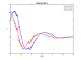
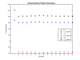
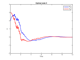
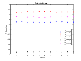
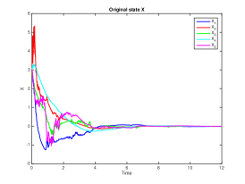
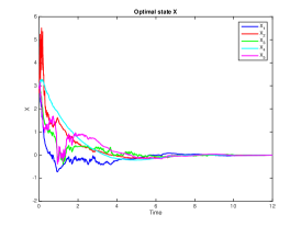
Figure 1: Simulation results for solutions. (a): System state trajectory $X$ initialized by an arbitrary stabilizer $K^{(0)}$ in $2$-dimensional case; (b): Evolution of $P^{*}$ parameters in $2$-dimensional case; (c): The optimal state trajectory $X^{*}$ with optimal control $u^{*}=K^{*}X^{*}$ in $2$-dimensional case; (d): Evolution of $\widehat{A}$ parameters in $2$-dimensional case; (e): System state trajectory $X$ initialized by an arbitrary stabilizer $K^{(0)}$ in $5$-dimensional case; (f): The optimal state trajectory $X^{*}$ with optimal control $u^{*}=K^{*}X^{*}$ in $5$-dimensional case.

Following [1], we consider an example with $n=5$, $m=2$, and $R=I$. To save space, we do not present the parameters of the problem, please see details in [1]. Firstly, we initialize a stabilizer

$$K^{(0)}=\begin{bmatrix}-0.2038&0.1082&0.3309&-0.5508&-0.2534\\ 0.3653&0.7350&0.8492&-0.8452&-0.5654\end{bmatrix}.$$

Then, we read the data of state trajectory $X=(X_{1},X_{2},X_{3},X_{4},X_{5})^{\top}$ with $K^{(0)}$, which is presented in Fig. 1 (e). By Algorithm 8, we get

$$P^{*}=\begin{bmatrix}0.3684&0.3093&0.2112&0.0272&-0.3673\\ 0.3093&1.3393&1.2834&-1.0028&-0.7576\\ 0.2112&1.2834&1.6839&-1.2101&-0.7842\\ 0.0272&-1.0028&-1.2101&2.0571&0.0801\\ -0.3673&-0.7576&-0.7842&0.0801&1.6467\end{bmatrix}$$

after $15$ iterations in $7$ seconds with

$$\small{\mathcal{R}(P^{*})=10^{-3}\cdot\begin{bmatrix}-0.2442&0.1120&-0.0145&0.0413&0.0391\\ 0.1120&0.0245&-0.1813&0.0381&0.0287\\ -0.0145&-0.1813&0.3078&0.0743&-0.0869\\ 0.0413&0.0381&0.0743&-0.1005&0.0014\\ 0.0391&0.0287&-0.0869&0.0014&0.2771\end{bmatrix},}$$

and $\|\mathcal{R}(P^{*})\|=6.0846\times 10^{-4}$. Comparatively, the accuracy of the corresponding result in [1] is $\|\mathcal{R}(P)\|=2.6\times 10^{-9}$. Because our RL method does not use any information of $A$ while the SDP method uses all the information of the system, the accuracy of the former is lower than the latter. The optimal control is $u^{*}=K^{*}X^{*}$, where

$$K^{*}=\begin{bmatrix}-0.3358&-0.1425&-0.0369&0.1088&-0.0435\\ 0.4476&0.8551&0.9530&-0.8889&-0.3945\end{bmatrix}.$$

The optimal state $X^{*}=(X^{*}_{1},X^{*}_{2},X^{*}_{3},X^{*}_{4},X^{*}_{5})^{\top}$ is presented in Fig. 1 (f).

References

- [1] M. Ait Rami and X. Y. Zhou, “Linear Matrix Inequalities, Riccati Equations, and Indefinite Stochastic Linear Quadratic Controls”, IEEE Trans. Automat. Contr., vol. 45, pp. 1131-1143, 2000.
- [2] L. C. III Baird, “Reinforcement learning in continuous time: Advantage updating”, In Proc. of ICNN, 1994.
- [3] L. D. Berkovitz,“Optimal Control Theory”, Springer-Verlag, New York, 1974.
- [4] S. J. Bradtke, B. E. Ydestie and A. G. Barto, “Adaptive linear quadratic control using policy iteration”, In: Proc. of ACC, pp. 3475-3476, 1994.
- [5] S. Chen, X. Li and X. Zhou, “Stochastic linear quadratic regulators with indefinite control weight costs”, SIAM J. Optimiz., vol. 36, pp. 1685-1702, 1998.
- [6] X. Chen, G. Qu, Y. Tang, S. Low and N. Li, “Reinforcement Learning for Decision-Making and Control in Power Systems: Tutorial, Review, and Vision”, arXiv preprint arXiv:2102.01168v3, 2021.
- [7] T. Bian and Z. Jiang, “Reinforcement Learning for Linear Continuous-time Systems: an Incremental Learning Approach”, IEEE-CAA J. Automatic., vol. 6, pp. 433-440, 2019.
- [8] T. E. Duncan, L. Guo and B. Pasik-Duncan, “Adaptive Continuous-Time Linear Quadratic Gaussian Control”, IEEE Trans. Automat. Contr., vol. 44, pp. 1653-1662, 1999.
- [9] M. Fazel, R. Ge, S. M. Kakade, and M. Mesbahi, “Global convergence of policy gradient methods for the linear quadratic regulator”, In Proc. Int’l Conf. Machine Learning, pp. 1467-1476, 2018.
- [10] W. H. Fleming and M. Nisio, “On stochastic relaxed control for partially observed diffusions”, Nagoya Mathematical Journal, vol. 93, pp. 71-108, 1984.
- [11] J. Huang, X. Li and J, Yong, “A Linear-Quadratic Optimal Control Problem for Mean-Field Stochastic Differential Equations in Infinite Horizon”, Math. Control Relat. F., vol. 5, pp. 97-139, 2015.
- [12] Y. Jiang and Z. Jiang, “Global adaptive dynamic programming for continuous-time nonlinear systems”, IEEE Trans. Automat. Contr., vol. 60, pp. 2917-2929, 2015.
- [13] B. Kiumarsi, K. G. Vamvoudakis, H. Modares, and F. L. Lewis, “Optimal and Autonomous Control Using Reinforcement Learning: A Survey”, IEEE T. Neur. Net. Lear., vol. 29, pp. 2042-2061, 2018.
- [14] B. Kiumarsia, B. AlQaudi, H. Modaresa, F. L. Lewis and D. S. Levinee, “Optimal control using adaptive resonance theory and Q-learning”, Neurocomputing, vol. 361, pp. 119-125, 2019.
- [15] J. Lee and R. S. Sutton, “Policy iterations for reinforcement learning problems in continuous time and space- Fundamental theory and methods”, Automatica, vol. 126, 109421, 2021.
- [16] B. Luo, D. Liu and H. Wu, “Adaptive Constrained Optimal Control Design for Data-Based Nonlinear Discrete-Time Systems With Critic-Only Structure”, IEEE T. Neur. Net. Lear., vol. 29, pp. 2099-2111, 2018.
- [17] H. Modares, F. L. Lewis and Z. Jiang, “Optimal Output-Feedback Control of Unknown Continuous-Time Linear Systems Using Off-policy Reinforcement Learning”, IEEE T. Cybernetics, vol. 46, pp. 2401-2410, 2016.
- [18] J. M. Mendel and R. W. McLaren, “Reinforcement learning control and pattern recognition systems”. In J. M. Mendel, and K. S. Fu, Adaptive, learning and pattern recognition systems: Theory and applications, New York: Academic Press, vol. 66, pp. 287-318, 1970.
- [19] H. Mohammadi, M. Soltanolkotabi and M. R. Jovanović, “Learning the model-free linear quadratic regulator via random search”, 2nd Annual Conference on Learning for Dynamics and Control: Proceedings of Machine Learning Research, vol. 120, pp. 1-9, 2020.
- [20] J. J. Murray, C. J. Cox, G. G. Lendaris and R. Saeks, “Adaptive dynamic programming”, IEEE T. Syst. Man Cy-S, vol. 32, pp. 140-153, 2002.
- [21] K. S. Narendra and L. S. Valavani, “Direct and Indirect Adaptive Control”, IFAC Proceedings Volumes, vol. 11, pp. 1981-1987, 1978.
- [22] S. A. A. Rizvi and Z. Lin, “Output Feedback Q-Learning Control for the Discrete-Time Linear Quadratic Regulator Problem”, IEEE T. Neur. Net. Lear., vol. 30, pp. 1523-1536, 2019.
- [23] J. Sun and J. Yong, “Stochastic Linear Quadratic Optimal Control Problems in Infinite Horizon”, Appl. Math. Optim., vol. 78, pp. 145-183, 2018.
- [24] R.S. Sutton, A.G. Barto, “Reinforcement learning: An introduction”, MIT Press, Cambridge, Second Edition, 2018.
- [25] R.S. Sutton, A.G. Barto and R.J. Williams, “Reinforcement learning is direct adaptive optimal control”, In: Proc. of ACC, pp. 2143-2146, 1991.
- [26] V. A. Ugrinovskii, “Robust control in the presence of stochastic uncertainty”, Int. J. Contr., vol. 71, pp. 219-237, 1998.
- [27] D. Vrabie, O. Pastravanu, M. Abu-Khalaf and F.L. Lewis, “Adaptive optimal control for continuous-time linear systems based on policy iteration”, Automatica, vol. 45, pp. 477-484, 2009.
- [28] H. Wang, T. Zariphopoulou and X. Y. Zhou, “Reinforcement learning in continuous time and space: A stochastic control approach”, Journal of Machine Learning Research, vol. 21, pp. 1-34, 2020.
- [29] H. Wang and X. Y. Zhou, “Continuous-time mean–variance portfolio selection: A reinforcement learning framework”, Mathematical Finance, vol. 30, pp. 1273-1308, 2020.
- [30] C. J. C. H. Watkins, “Learning from delayed rewards”. Ph.D. thesis. England: University of Cambridge, 1989.
- [31] P. Werbos, “Neural networks for control and system identification”, In: Proc. of CDC, pp. 260-265, 1989.
- [32] W. Ch. Wong and J. H. Lee, “A reinforcement learning-based scheme for direct adaptive optimal control of linear stochastic systems”, Optimal Control Applications and Methods, vol. 31, pp. 365-374, 2010.
- [33] F. A. Yaghmaie and D. J. Braun, “Reinforcement learning for a class of continuous-time input constrained optimal control problems”, Automatica, vol. 99, pp. 221-227, 2019.
- [34] J. Yong and X. Y. Zhou, Stochastic controls: Hamiltonian systems and HJB equations, Applications of Mathematics (New York), 43, Springer-Verlag, New York, 1999.
- [35] X. Y. Zhou, “On the existence of optimal relaxed controls of stochastic partial differential equations”, SIAM J. Optimiz., vol. 30, pp. 247-261, 1992.