An efficient implementable inexact entropic proximal point algorithm for a class of linear programming problems

Abstract

We introduce a class of specially structured linear programming (LP) problems, which has favorable modeling capability for important application problems in different areas such as optimal transport, discrete tomography and economics. To solve these generally large-scale LP problems efficiently, we design an implementable inexact entropic proximal point algorithm (iEPPA) combined with an easy-to-implement dual block coordinate descent method as a subsolver. Unlike existing entropy-type proximal point algorithms, our iEPPA employs a more practically checkable stopping condition for solving the associated subproblems while achieving provable convergence. Moreover, when solving the capacity constrained multi-marginal optimal transport (CMOT) problem (a special case of our LP problem), our iEPPA is able to bypass the underlying numerical instability issues that often appear in the popular entropic regularization approach, since our algorithm does not require the proximal parameter to be very small in order to obtain an accurate approximate solution. Numerous numerical experiments show that our iEPPA is efficient and robust for solving large-scale CMOT problems. The experiments on the discrete tomography problem also highlight the potential modeling power of our model.

Keywords:  Linear programming; proximal point algorithm; entropic proximal term; block coordinate descent; capacity constrained multi-marginal optimal transport.

1 Introduction

In this paper, we introduce a class of specially structured linear programming (LP) problems of the following form:

$$\min \;\;\langle C,\,X\rangle$$ (1.1)

s.t. $$\;\;X\in\Omega:=\Big{\{}X\in\mathbb{R}^{n_{1}\times n_{2}\times n_{3}}~{}:~{}{\cal A}^{(i)}(X)\;=\;\bm{b}^{(i)},\quad i=1,\dots,N,\quad 0\leq X\leq U\Big{\}},$$

where $\langle\cdot,\cdot\rangle$ denotes the standard inner product in $\mathbb{R}^{n_{1}\times n_{2}\times n_{3}}$, ${\cal A}^{(i)}:\mathbb{R}^{n_{1}\times n_{2}\times n_{3}}\to\mathbb{R}^{m_{i}}$ is a given linear mapping defined by

$${\cal A}^{(i)}(X):=\left[\begin{array}[]{c}\langle A^{(i)}_{1},\,X\rangle\\ \vdots\\ \langle A^{(i)}_{m_{i}},\,X\rangle\end{array}\right],\quad A_{j}^{(i)}\in\mathbb{R}^{n_{1}\times n_{2}\times n_{3}},\quad 1\leq j\leq m_{i},\quad 1\leq i\leq N,$$

$\bm{b}^{(i)}=(b^{(i)}_{1},\dots,b^{(i)}_{m_{i}})^{\top}\in\mathbb{R}^{m_{i}}$ ($i=1,\dots,N$), $C\in\mathbb{R}^{n_{1}\times n_{2}\times n_{3}}$ and $U\in\mathbb{R}_{+}^{n_{1}\times n_{2}\times n_{3}}\cup\{\infty\}^{n_{1}\times n_{2}\times n_{3}}$ are given data. Moreover, the linear mappings ${\cal A}^{(i)}$ ($i=1,\dots,N$) satisfy Assumption 1 below. As we shall see shortly, problem (1.1) is a generalization of the classical discrete optimal transport problem which has the form: $\min\big{\{}\langle C,\,X\rangle:X\in\mathbb{R}^{n_{1}\times n_{2}},\,\sum_{s=1}^{n_{2}}X_{rs}=a_{r},\,r=1,\ldots,n_{1},\,\sum_{r=1}^{n_{1}}X_{rs}=b_{s},\,s=1,\ldots,n_{2},\,X\geq 0\big{\}}$, where $\bm{a}:=(a_{1},\dots,a_{n_{1}})^{\top}$ and $\bm{b}:=(b_{1},\dots,b_{n_{2}})^{\top}$ are two given marginals in $n_{1}$ and $n_{2}$-dimensional simplices, and $C\in\mathbb{R}^{n_{1}\times n_{2}}$ is a given cost matrix.

Assumption 1.

For each fixed $i$ ($1\leq i\leq N$), $A_{j}^{(i)}$ only has binary entries (0 or 1) for $j=1,\dots,m_{i}$, and the given constraint tensors $\big{\{}A_{j}^{(i)}\;|\;j=1,\dots,m_{i}\big{\}}$ satisfy the property that

$$A_{j}^{(i)}\circ A_{k}^{(i)}=0,\quad\text{if }~{}j\neq k,\;j,\,k=1,\dots,m_{i},$$

where “$\circ$” denotes the Hadamard product.

The property stated in Assumption 1 is equivalent to saying that the non-zero patterns of any two distinct constraint tensors $A^{(i)}_{j}$ and $A^{(i)}_{k}$ do not overlap in the $i$-block of the linear constraints ${\cal A}^{(i)}(X)=\bm{b}^{(i)}$. Such structures may look unusual at the first glance, but do appear in a few important application problems, for example, the capacity constrained multi-marginal optimal transport (CMOT) problem with three marginals, the discrete tomography problem [1, 7, 42], the disaggregation of industry-by-industry input-output tables in economics [20], and reconstructions of unknown inter-bank liabilities with fixed constraints [18]; see details on first two examples in the next two paragraphs. Moreover, as we shall see later, such special structures allow us to design a highly efficient algorithm to solve the corresponding LPs since they can greatly facilitate the computations of the subproblems involved in our algorithm; see Section 3 and Appendix A for more details.

The discrete 3-marginal CMOT problem is modeled as follows:

$$\min\limits_{X\in\mathbb{R}^{n_{1}\times n_{2}\times n_{3}}}\,\,\,\langle C,\,X\rangle$$ (1.2)

$$\hskip 22.76228pt\mathrm{s.t.}\hskip 11.38092pt\begin{array}[]{lll}&{\textstyle\sum_{s,t}}X_{rst}=a_{r},~{}r=1,\dots,n_{1},&{\textstyle\sum_{r,t}}X_{rst}=b_{s},~{}s=1,\dots,n_{2},\\[5.0pt] &{\textstyle\sum_{r,s}}X_{rst}=c_{t},~{}t=1,\dots,n_{3},&0\leq X\leq U,\end{array}$$

where $\bm{a}:=(a_{1},\dots,a_{n_{1}})^{\top}\in\Sigma_{n_{1}}$, $\bm{b}:=(b_{1},\dots,b_{n_{2}})^{\top}\in\Sigma_{n_{2}}$, $\bm{c}:=(c_{1},\dots,c_{n_{3}})^{\top}\in\Sigma_{n_{3}}$ are three given marginals with $\Sigma_{n_{i}}$ denoting the $n_{i}$-dimensional unit simplex for $i=1,\,2,\,3$. When $n_{3}=1$, the above problem readily reduces to the classical optimal transport problem mentioned in the first paragraph, but with an additional upper bound constraint. It is clear that problem (1.2) falls into the form of (1.1) with

$$A^{(1)}_{j} =\bm{e}_{j}^{(1)}\otimes\bm{1}_{n_{2}}\otimes\bm{1}_{n_{3}},\quad j=1,\dots,n_{1},$$ (1.3)

$$A^{(2)}_{j} =\bm{1}_{n_{1}}\otimes\bm{e}_{j}^{(2)}\otimes\bm{1}_{n_{3}},\quad j=1,\dots,n_{2},$$

$$A^{(3)}_{j} =\bm{1}_{n_{1}}\otimes\bm{1}_{n_{2}}\otimes\bm{e}_{j}^{(3)},\quad j=1,\dots,n_{3},$$

where $\bm{e}_{j}^{(i)}$ denotes the $j$th unit vector in $\mathbb{R}^{n_{i}}$ ($i=1,\,2,\,3$), $\bm{1}_{n_{i}}$ denotes the $n_{i}$-dimensional vector of all ones for $i=1,\,2,\,3$, and “$\otimes$” denotes the tensor product (see the definition at the end of this section). Problem (1.2) was first proposed and studied by Korman and McCann [24, 25] in the 2-marginal continuous case as an important variant of the classical 2-marginal optimal transport (OT) problem. This variant takes into account limits on the transport capacities via imposing a proper upper bound constraint $X\leq U$, and hence it is better able to model some real-life situations. Moreover, we note that if the constraints in (1.2) are summed over a single index instead of two indices (for example, $\sum_{s}X_{rst}=a_{rt}$ for $r=1,\ldots,n_{1}$, $t=1,\ldots,n_{3}$), then the resulting problem can model a multi-commodity flow problem on a bipartite graph, where the commodities are indexed by $t=1,\ldots,n_{3}$; see, for example, [23].

In the 2-dimensional discrete tomography problem studied in [42], one is given the marginals obtained from an $n\times n$ matrix (for simplicity, we discuss the matrix case instead of a third-order tensor) by summing its entries along different directions, for example, $0^{\circ}$, $45^{\circ}$, $90^{\circ}$ and $135^{\circ}$ directions. In this case, the formulation in [1] would require a sixth-order tensor to model the problem as a 6-marginal optimal transport problem. Unfortunately, this approach leads to an exponential increase in the computational cost because of the curse of dimensionality brought about by the extra dimensions introduced in the higher-order tensor. But using our model in (1.1), the variable remains as a matrix and the projections along the four directions are formulated as four blocks of linear constraints, each represented by a linear mapping ${\cal A}^{(i)}(X)=\bm{b}^{(i)}$ with $\bm{b}^{(i)}$ being the given $i$th marginal for $i=1,\dots\!,4$. Moreover, it is not hard to verify that the constraint matrices associated with each linear mapping ${\cal A}^{(i)}$ satisfy Assumption 1. For the construction of a block of linear constraints that represents a projection along a specific direction, we refer the reader to subsection 4.3 and Appendix C.

Note that problem (1.1) has $n_{1}n_{2}n_{3}$ box-constrained variables and $\sum_{i=1}^{N}m_{i}$ linear equality constraints, and thus it is usually a very large-scale LP problem when the dimension of the variable or the number of blocks of linear constraints is large. Therefore, classical LP methods such as the simplex method and the interior point method may no longer be efficient enough or may consume too much memory when solving this problem. Recently, an entropic regularized approach was proposed in [6] to approximately solve problem (1.2) in the 2-marginal case with impressive numerical performance. This approach basically modifies the original LP problem by adding an entropic regularization to the objective, and then applies a certain efficient first-order method to solve the resulting computationally more tractable regularized problem to obtain an approximate solution of the original LP problem. In [6], Dykstra’s algorithm with Kullback-Leibler projections (DyKL) is adapted to solve the entropic regularized counterpart of problem (1.2) in the 2-marginal case (see (B.1)). This algorithm can be highly efficient if a crude approximate solution is adequate, in which case the regularization parameter needs not be very small. However, when one decreases the regularization parameter to a small value for obtaining a more accurate solution, the DyKL would encounter the difficulties of numerical instabilities (due to loss of accuracy involving overflow/underflow operations) and slow convergence speed, just as Sinkhorn’s algorithm [37] employed in [13] for approximately solving the classical 2-marginal OT problem. Though the former difficulty can partially be alleviated by some stabilization techniques (e.g., applying the log-sum-exp operation [32, Section 4.4]) at the expense of losing some computational efficiency, the latter difficulty of slow convergence, however, is unavoidable when the regularization parameter is small, as clearly observed from our numerical experiments in Section 4. In addition, we are not aware of fast algorithms that are specifically designed for solving the more general problem (1.1).

In this paper, we develop an implementable inexact entropic proximal point algorithm (iEPPA) for solving problem (1.1). Our iEPPA falls into the family of Bregman-distance-based PPA [11, 12, 15, 16] and the family of $\phi$-divergence-based PPA [3, 17, 21, 22, 38, 39], both of which have been widely studied in the literature, especially in the 1990’s starting from the paper [11]. However, we should point out that we have made an essential change to the algorithm by introducing a more practical stopping condition (2.3) for solving the subproblems. Therefore, existing convergence results may not be applicable and the convergence analysis has to be re-established for our iEPPA; see Theorem 1. Moreover, as a byproduct, we actually develop a unified inexact framework for EPPA including Teboulle’s framework [39] and Eckstein’s framework [16] as special cases. This makes our iEPPA more flexible. To solve the subproblem (2.2), we first derive its dual problem and characterize the properties of its optimal solutions in Section 3. We then apply a block coordinate descent (BCD) method to solve the resulting dual problem and establish the linear convergence by revisiting some classical results for the BCD method in [28, 29, 41]. We also show how the subproblems in the BCD method can be solved efficiently under Assumption 1. In particular, no stabilization technique is needed for the BCD updates since our iEPPA does not require a small proximal parameter in each iteration. This is indeed a key advantage of our iEPPA over the popular entropic regularization approach in [6]. Recently, a similar algorithmic framework studied by Eckstein [16] was also adapted in [43] for solving the classical OT problem with encouraging numerical performance. However, the algorithm there was developed under a rather stringent inexact condition, which is nontrivial to verify or implement in practice.

The contributions of this paper are summarized as follows.

• We introduce a class of specially structured LP problems (1.1), which covers some important existing problems and has favorable modeling capability. For example, it is able to formulate a tomography problem without using a high-order tensor. This is in contrast to [1, 7] where a high-order (equals to two plus the number of projection directions) tensor is used to model a 2D tomography problem, and consequently the resulting problem is extremely large-scale and prohibitively expensive to solve in terms of both memory consumption and computational cost. In addition, the third-order tensor model (1.1) and the subsequent algorithms can naturally be extended to higher-order cases if needed.

• We develop an efficient iEPPA combined with a dual BCD method, namely, iEPPA+BCD, to solve the proposed structured LP problem (1.1). It has the important strength of being able to faithfully solve the original problem without requiring the proximal parameter to be very small. As a result, when solving the CMOT problem (1.2), it can bypass the inherent numerical instabilities that often plague the entropic regularization approach. While our iEPPA+BCD framework is not completely new but a novel combination of existing algorithms in the optimization literature, we have nevertheless introduced an essential modification to make the algorithm practically implementable by proposing a computationally checkable stopping condition for finding a sufficiently accurate approximate solution of the subproblem in each iEPPA iteration to ensure the convergence of the overall algorithm.

• We conduct rigorous numerical experiments to illustrate the efficiency of our iEPPA+BCD framework for solving the CMOT problem (1.2), in comparison to the (stabilized) DyKL and the powerful commercial solver Gurobi. Experiments on the discrete tomography problem also show the favorable modeling power of our model.

The rest of this paper is organized as follows. The iEPPA for solving problem (1.1) and its convergence results are described in Section 2. The dual BCD method for solving the subproblem and its convergence analysis are presented in Section 3. Moreover, the details on the implementable verification of our new inexact condition is also included in Section 3. Extensive numerical results are reported in Section 4, with some concluding remarks given in Section 5.

Notation and Preliminaries

The elements of a third-order tensor $X\in\mathbb{R}^{n_{1}\times n_{2}\times n_{3}}$ are denoted as $X_{rst}$ where $1\leq r\leq n_{1},\;1\leq s\leq n_{2},\;1\leq t\leq n_{3}$. For any tensors $X$, $Y\in\mathbb{R}^{n_{1}\times n_{2}\times n_{3}}$, we define their inner product as $\langle X,\,Y\rangle:={\textstyle\sum_{r=1}^{n_{1}}\sum_{s=1}^{n_{2}}\sum_{t=1}^{n_{3}}}\,X_{rst}\,Y_{rst}$. The Frobenius norm of $X$ is defined by $\|X\|_{F}:=\sqrt{\langle X,\,X\rangle}$. For any $X$, $Y\in\mathbb{R}^{n_{1}\times n_{2}\times n_{3}}$, the Hadamard product of $X$ and $Y$ is defined by $(X\circ Y)_{rst}:=X_{rst}\,Y_{rst}$ for any $1\leq r\leq n_{1}$, $1\leq s\leq n_{2}$, $1\leq t\leq n_{3}$. Similarly, we use “$./$” to denote the element-wise division operator. We use “$\otimes$” to denote the tensor product of vectors. Specifically, let $\bm{u}^{(i)}\in\mathbb{R}^{n_{i}}$ ($i=1,\,2,\,3$) be three arbitrary column vectors. Their tensor product is denoted by $\bm{u}^{(1)}\otimes\bm{u}^{(2)}\otimes\bm{u}^{(3)}\in\mathbb{R}^{n_{1}\times n_{2}\times n_{3}}$ whose elements are given by $(\bm{u}^{(1)}\otimes\bm{u}^{(2)}\otimes\bm{u}^{(3)})_{rst}:=u^{(1)}_{r}u^{(2)}_{s}u^{(3)}_{t}$ for any $1\leq r\leq n_{1}$, $1\leq s\leq n_{2}$, $1\leq t\leq n_{3}$.

Let $\mathbb{E}$ be a finitely dimensional real Euclidean space equipped with an inner product $\langle\cdot,\cdot\rangle$ and its induced norm $\|\cdot\|$. For an extended-real-valued function $f:\mathbb{E}\rightarrow[-\infty,\infty]$, we say that it is proper if $f(\bm{x})>-\infty$ for all $\bm{x}\in\mathbb{E}$ and its domain ${\rm dom}\,f:=\{\bm{x}\in\mathbb{E}:f(\bm{x})<\infty\}$ is nonempty. A proper function $f$ is said to be closed if it is lower semicontinuous. Assume that $f:\mathbb{E}\rightarrow(-\infty,\infty]$ is a proper closed convex function. For a given $\nu\geq 0$, the $\nu$-subdifferential of $f$ at $\bm{x}\in{\rm dom}\,f$ is defined by $\partial_{\nu}f(\bm{x}):=\{\bm{d}\in\mathbb{E}:f(\bm{y})\geq f(\bm{x})+\langle\bm{d},\,\bm{y}-\bm{x}\rangle-\nu,~{}\forall\,\bm{y}\in\mathbb{E}\}$ and when $\nu=0$, $\partial_{\nu}f$ is simply denoted by $\partial f$, which is referred to as the subdifferential of $f$. The conjugate function of $f$ is $f^{*}:\mathbb{E}\rightarrow(-\infty,\infty]$ defined by $f^{*}(\bm{y}):=\sup\left\{\langle\bm{y},\,\bm{x}\rangle-f(\bm{x}):\bm{x}\in\mathbb{E}\right\}$. For any $\bm{x}$, $\bm{y}\in\mathbb{E}$, it follows from [34, Theorem 23.5] that

$$\bm{y}\in\partial f(\bm{x})~{}~{}\Longleftrightarrow~{}~{}\bm{x}\in\partial f^{*}(\bm{y}).$$ (1.4)

Moreover, we call a proper closed convex function $f$ essentially smooth if (i) the interior of $\mathrm{dom}\,f$, denoted by $\mathrm{int}\,\mathrm{dom}\,f$, is not empty; (ii) $f$ is differentiable on $\mathrm{int}\,\mathrm{dom}\,f$; (iii) $\|\nabla f(x_{k})\|\to\infty$ for every sequence $\{x_{k}\}$ in $\mathrm{int}\,\mathrm{dom}\,f$ converging to a boundary point of $\mathrm{int}\,\mathrm{dom}\,f$; see [34, page 251].

Finally, we make a blanket assumption throughout this paper.

Assumption 2.

The feasible set $\Omega$ is bounded and $\Omega\cap\mathbb{R}^{n_{1}\times n_{2}\times n_{3}}_{++}$ is nonempty.

This assumption ensures the well-definedness of problem (1.1) and our method developed in the next section. The boundedness assumption can be satisfied if, for instance, $U\in\mathbb{R}_{+}^{n_{1}\times n_{2}\times n_{3}}$ or the constraints are given as in (1.2).

2 An implementable inexact entropic proximal point algorithm

In this section, we develop an implementable inexact entropic proximal point algorithm (iEPPA) for solving problem (1.1). To describe the iterates of the iEPPA, we first rewrite problem (1.1) as follows:

$$\min\limits_{X}~{}\delta_{\Omega^{\circ}}(X)+\langle{C},\,X\rangle,\quad\mathrm{s.t.}\quad X\geq 0,$$ (2.1)

where $\delta_{\Omega^{\circ}}(\cdot)$ is the indicator function of the set $\Omega^{\circ}$ defined as

$$\Omega^{\circ}:=\big{\{}X\in\mathbb{R}^{n_{1}\times n_{2}\times n_{3}}~{}:~{}{\cal A}^{(i)}(X)=\bm{b}^{(i)},~{}i=1,\dots,N,~{}X\leq U\big{\}}.$$

Obviously, the set $\Omega^{\circ}$ is formed by removing the non-negative constraint on $X$ from the set $\Omega$ and hence $\Omega\subseteq\Omega^{\circ}$. We also introduce the Boltzmann-Shannon entropy function $\phi(X)=\sum_{rst}X_{rst}\log X_{rst}-X_{rst}$ (with the convention that $0\log 0=0$) and its conjugate function $\phi^{*}(Y)=\sum_{rst}\exp(Y_{rst})$. Then, the Bregman distance [9] with $\phi$ as the kernel function, is defined as

$$\mathcal{D}_{\phi}(X,\,Y):=\phi(X)-\phi(Y)-\langle\nabla\phi(Y),\,X-Y\rangle,\quad\forall\,X\in\mathbb{R}_{+}^{n_{1}\times n_{2}\times n_{3}},~{}Y\in\mathbb{R}_{++}^{n_{1}\times n_{2}\times n_{3}}.$$

It is easy to see that $D_{\phi}(X,\,Y)\geq 0$ and the equality holds if and only if $X=Y$. Then, the iEPPA for solving (2.1) (hence (1.1)) is presented as Algorithm 1.

Algorithm 1 An implementable inexact entropic proximal point algorithm (iEPPA) for solving (2.1)

Input: Let $\{\varepsilon_{k}\}_{k=0}^{\infty}$, $\{\nu_{k}\}_{k=0}^{\infty}$, $\{\eta_{k}\}_{k=0}^{\infty}$ and $\{\mu_{k}\}_{k=0}^{\infty}$ be four sequences of nonnegative scalars. Choose $X^{0}=\widetilde{X}^{0}\in\mathbb{R}_{++}^{n_{1}\times n_{2}\times n_{3}}$ arbitrarily. Set $k=0$.
while the termination criterion is not met, do

• Find a pair $(X^{k+1},\,\widetilde{X}^{k+1})$ by approximately solving the following problem

  $$\min\limits_{X}~{}\delta_{\Omega^{\circ}}(X)+\langle C,\,X\rangle+\varepsilon_{k}\,\mathcal{D}_{\phi}(X,\,X^{k}),$$ (2.2)

  such that $X^{k+1}\in\mathbb{R}_{++}^{n_{1}\times n_{2}\times n_{3}}$, $\widetilde{X}^{k+1}\in\Omega$ and

  $$\Delta^{k}\in\partial_{\nu_{k}}\delta_{\Omega^{\circ}}(\widetilde{X}^{k+1})+C+\varepsilon_{k}\,\big{(}\nabla\phi(X^{k+1})-\nabla\phi(X^{k})\big{)}$$ (2.3)

  $$\quad\mathrm{with}~{}~{}\|\Delta^{k}\|_{F}\leq\eta_{k},~{}~{}\mathcal{D}_{\phi}(\widetilde{X}^{k+1},\,X^{k+1})\leq\mu_{k}.$$

• Set $k=k+1$ and go to Step 1.

end while
Output: $(X^{k},\,\widetilde{X}^{k})$

The reader may have observed that the iEPPA in Algorithm 1 basically solves the original problem (2.1) (hence (1.1)) via approximately solving a sequence of subproblems (2.2) each involving a special entropic Bregman proximal term. Since $\mathrm{dom}\,\phi=\mathbb{R}_{+}^{n_{1}\times n_{2}\times n_{3}}$, the constraint $X\geq 0$ can be removed in (2.2). Moreover, the Boltzmann-Shannon entropy function $\phi(X)=\sum_{rst}X_{rst}\log X_{rst}-X_{rst}$ is essentially smooth and strictly convex on $\mathbb{R}_{+}^{n_{1}\times n_{2}\times n_{3}}$. This together with Assumption 2 ensures that each subproblem (2.2) is well-defined in the sense that its optimal solution (denoted by $X^{k,*}$) uniquely exists and lies in $\mathbb{R}_{++}^{n_{1}\times n_{2}\times n_{3}}$. Indeed, since $\Omega^{\circ}\cap\mathrm{dom}\,\phi=\Omega$ is bounded, the objective function in subproblem (2.2) is then level-bounded. Thus, a solution exists [35, Theorem 1.9] and must be unique since $\phi$ is strictly convex. The essential smoothness of $\phi$ and Assumption 2 further imply that $X^{k,*}$ can only lie in $\mathbb{R}_{++}^{n_{1}\times n_{2}\times n_{3}}$. Notice that our inexact condition (2.3) always holds when $X^{k+1}=\widetilde{X}^{k+1}=X^{k,*}$ and hence it is achievable.

The inexact condition (2.3) is rather general to cover some existing inexact conditions, and more importantly, it makes our iEPPA more practical for solving problem (2.1) (hence (1.1)). When $\nu_{k}\equiv\eta_{k}\equiv\mu_{k}\equiv 0$, $X^{k+1}$ (equals to $\widetilde{X}^{k+1}$) must be the exact optimal solution of subproblem (2.2). In this case, our exact version of iEPPA is indeed a special case of the classical exact generalized PPA (such as the $\phi$-divergence-based PPA [3, 17, 21, 22, 38] and the Bregman-distance-based PPA [11, 12, 15]). When $\eta_{k}\equiv\mu_{k}\equiv 0$, condition (2.3) reduces to

$$0\in\partial_{\nu_{k}}\delta_{\Omega^{\circ}}(X^{k+1})+C+\varepsilon_{k}\big{(}\nabla\phi(X^{k+1})-\nabla\phi(X^{k})\big{)},$$ (2.4)

which is considered by Teboulle [39] in the $\phi$-divergence-based PPA that allows the approximate computations of the subdifferential of $\delta_{\Omega^{\circ}}$ at $X^{k+1}$, provided $X^{k+1}\in\Omega^{\circ}$. When $\nu_{k}\equiv\mu_{k}\equiv 0$, condition (2.3) reduces to

$$\Delta^{k}\in\partial\delta_{\Omega^{\circ}}(X^{k+1})+C+\varepsilon_{k}\big{(}\nabla\phi(X^{k+1})-\nabla\phi(X^{k})\big{)}~{}~{}\mathrm{with}~{}~{}\|\Delta^{k}\|_{F}\leq\eta_{k},$$ (2.5)

which is considered by Eckstein [16] in the Bregman-distance-based PPA and is typically easier to check than the $\nu$-subdifferential-based condition (2.4). But again, it requires $X^{k+1}$ to be in $\Omega^{\circ}$. The inexact algorithmic framework based on condition (2.5) has also been adapted in [43] for solving the classical 2-marginal OT problem. However, we should mention that neither Teboulle’s inexact condition (2.4) nor Eckstein’s inexact condition (2.5) is easy to implement for solving the subproblem with the complicated constraint that $X\in\Omega^{\circ}$. Because it is nontrivial to find a point $X^{k+1}$ that simultaneously satisfies $X^{k+1}\in\Omega^{\circ}$ (required by the nonemptyness of $\partial_{\nu_{k}}\delta_{\Omega^{\circ}}(X^{k+1})$ or $\partial\delta_{\Omega^{\circ}}(X^{k+1})$) and $X^{k+1}\in\mathbb{R}_{++}^{n_{1}\times n_{2}\times n_{3}}$ (required by the essentially smoothness of $\phi$). This inadequacy thus motivated us to further relax conditions (2.4) and (2.5) to condition (2.3), in which $\partial_{\nu_{k}}\delta_{\Omega^{\circ}}$ and $\nabla\phi$ are allowed to be computed at two slightly different points, respectively. We shall show later in subsection 3.2 that the verification of our inexact condition (2.3) is more practically implementable.

We next establish the convergence of our iEPPA in Algorithm 1. Our analysis is inspired by several existing works (see, for example, [16, 39]), but is more involved due to the flexible inexact condition (2.3). We shall start with some elementary preliminaries. It is known from [10, Section 6.1] that the Boltzmann-Shannon entropy function $\phi$ has many elegant properties as a Bregman function (see [10, Definition 2.1]). We point out three of them below that are useful in our subsequential analysis. More details on the Bregman function can be found in [4, Section 4].

Property 1.

The following properties hold for $\phi(X)=\sum_{rst}X_{rst}\log X_{rst}-X_{rst}$.

• For any $X\in\mathbb{R}_{+}^{n_{1}\times n_{2}\times n_{3}}$, $\mathcal{D}_{\phi}(X,\,\cdot)$ is level-bounded.

• If $\{Y^{k}\}\subseteq\mathbb{R}_{++}^{n_{1}\times n_{2}\times n_{3}}$ converges to some $Y^{*}\in\mathbb{R}_{+}^{n_{1}\times n_{2}\times n_{3}}$, then $\mathcal{D}_{\phi}(Y^{*},\,Y^{k})\to 0$.

• (Convergence consistency) If $\{X^{k}\}\subseteq\mathbb{R}_{+}^{n_{1}\times n_{2}\times n_{3}}$ and $\{Y^{k}\}\subseteq\mathbb{R}_{++}^{n_{1}\times n_{2}\times n_{3}}$ are two sequences such that $\{X^{k}\}$ is bounded, $Y^{k}\to Y^{*}$ and $\mathcal{D}_{\phi}(X^{k},\,Y^{k})\to 0$, then $X^{k}\to Y^{*}$.

We also recall two well-known results.

Lemma 1 (Three points identity [12, Lemma 3.1]).

For any $X\in\mathbb{R}^{n_{1}\times n_{2}\times n_{3}}_{+}$ and $Y,\,Z\in\mathbb{R}^{n_{1}\times n_{2}\times n_{3}}_{++}$, the following identity holds:

$$\langle\nabla\phi(Y)-\nabla\phi(Z),\,X-Y\rangle=\mathcal{D}_{\phi}(X,\,Z)-\mathcal{D}_{\phi}(X,\,Y)-\mathcal{D}_{\phi}(Y,\,Z).$$

Lemma 2 ([33, Section 2.2]).

Suppose that $\{a_{k}\}_{k=0}^{\infty}\subseteq\mathbb{R}$ and $\{\gamma_{k}\}_{k=0}^{\infty}\subseteq\mathbb{R}$ are two sequences such that $\{a_{k}\}$ is bounded from below, $\sum_{k=0}^{\infty}\gamma_{k}<\infty$, and $a_{k+1}\leq a_{k}+\gamma_{k}$ holds for all $k$. Then, $\{a_{k}\}$ is convergent.

We are now ready to give the main convergence result.

Theorem 1 (Convergence of the iEPPA).

Suppose that Assumption 2 holds and $\{\varepsilon_{k}\}_{k=0}^{\infty}$, $\{\nu_{k}\}_{k=0}^{\infty}$, $\{\eta_{k}\}_{k=0}^{\infty}$, $\{\mu_{k}\}_{k=0}^{\infty}$ are four sequences of nonnegative scalars. Let $\{X^{k}\}$ and $\{\widetilde{X}^{k}\}$ be the sequences generated by the iEPPA in Algorithm 1. If $0<\underline{\varepsilon}\leq\varepsilon_{k}\leq\bar{\varepsilon}<\infty$, $\sum\nu_{k}<\infty$, $\sum\eta_{k}<\infty$ and $\sum\mu_{k}<\infty$, then $\{X^{k}\}$ and $\{\widetilde{X}^{k}\}$ converge to a same optimal solution of problem (2.1) (hence problem (1.1)).

Proof.

First, from condition (2.3), there exists a $D^{k+1}\in\partial_{\nu_{k}}\delta_{\Omega^{\circ}}(\widetilde{X}^{k+1})$ such that

$$\Delta^{k}=D^{k+1}+C+\varepsilon_{k}\big{(}\nabla\phi(X^{k+1})-\nabla\phi(X^{k})\big{)}.$$

Then, for any $P\in\Omega\subseteq\Omega^{\circ}$, we see that

$$0\geq\langle D^{k+1},\,P-\widetilde{X}^{k+1}\rangle-\nu_{k}=\langle\Delta^{k}-C-\varepsilon_{k}\big{(}\nabla\phi(X^{k+1})-\nabla\phi(X^{k})\big{)},\,P-\widetilde{X}^{k+1}\rangle-\nu_{k},$$

which implies that

$$\langle C,\,\widetilde{X}^{k+1}\rangle\leq\langle C,\,P\rangle+\varepsilon_{k}\langle\,\nabla\phi(X^{k+1})-\nabla\phi(X^{k}),\,P-\widetilde{X}^{k+1}\,\rangle+\langle\Delta^{k},\,\widetilde{X}^{k+1}-P\rangle+\nu_{k}.$$ (2.6)

Note that

$$\quad\;\langle\,\nabla\phi(X^{k+1})-\nabla\phi(X^{k}),\,P-\widetilde{X}^{k+1}\,\rangle$$ (2.7)

$$=\langle\,\nabla\phi(X^{k+1})-\nabla\phi(X^{k}),\,P-X^{k+1}\,\rangle-\langle\,\nabla\phi(X^{k+1})-\nabla\phi(X^{k}),\,\widetilde{X}^{k+1}-X^{k+1}\,\rangle$$

$$=\mathcal{D}_{\phi}(P,\,X^{k})-\mathcal{D}_{\phi}(P,\,X^{k+1})-\mathcal{D}_{\phi}(X^{k+1},\,X^{k})-\big{(}\mathcal{D}_{\phi}(\widetilde{X}^{k+1},\,X^{k})-\mathcal{D}_{\phi}(\widetilde{X}^{k+1},\,X^{k+1})-\mathcal{D}_{\phi}(X^{k+1},\,X^{k})\big{)}$$

$$=\mathcal{D}_{\phi}(P,\,X^{k})-\mathcal{D}_{\phi}(P,\,X^{k+1})-\mathcal{D}_{\phi}(\widetilde{X}^{k+1},\,X^{k})+\mathcal{D}_{\phi}(\widetilde{X}^{k+1},\,X^{k+1})$$

$$\leq\mathcal{D}_{\phi}(P,\,X^{k})-\mathcal{D}_{\phi}(P,\,X^{k+1})-\mathcal{D}_{\phi}(\widetilde{X}^{k+1},\,X^{k})+\mu_{k},$$

where the second equality follows from the three points identity in Lemma 1. Moreover, since $\widetilde{X}^{k+1}\in\Omega$ and $P\in\Omega$, then $\langle\Delta^{k},\,\widetilde{X}^{k+1}-P\rangle\leq\|\widetilde{X}^{k+1}-P\|_{F}\|\Delta^{k}\|_{F}\leq 2\rho\eta_{k}$, where the last inequality follows from the boundedness of $\Omega$ (by Assumption 2) and hence there exists a $\rho>0$ such that $\|X\|_{F}\leq\rho$ for all $X\in\Omega$. Combining this with (2.6) and (2.7), we have

$$\langle C,\,\widetilde{X}^{k+1}\rangle\leq\langle C,\,P\rangle+\varepsilon_{k}\big{(}\mathcal{D}_{\phi}(P,\,X^{k})-\mathcal{D}_{\phi}(P,\,X^{k+1})-\mathcal{D}_{\phi}(\widetilde{X}^{k+1},\,X^{k})\big{)}+\varepsilon_{k}\mu_{k}+2\rho\eta_{k}+\nu_{k},~{}~{}\forall\,P\in\Omega.$$ (2.8)

Now, set $P=\widetilde{X}^{k}$ in (2.8), we see that

$$\langle C,\,\widetilde{X}^{k+1}\rangle \leq\langle C,\,\widetilde{X}^{k}\rangle+\varepsilon_{k}\big{(}\mathcal{D}_{\phi}(\widetilde{X}^{k},\,X^{k})-\mathcal{D}_{\phi}(\widetilde{X}^{k},\,X^{k+1})-\mathcal{D}_{\phi}(\widetilde{X}^{k+1},\,X^{k})\big{)}+\varepsilon_{k}\mu_{k}+2\rho\eta_{k}+\nu_{k}$$ (2.9)

$$\leq\langle C,\,\widetilde{X}^{k}\rangle-\varepsilon_{k}\big{(}\mathcal{D}_{\phi}(\widetilde{X}^{k},\,X^{k+1})+\mathcal{D}_{\phi}(\widetilde{X}^{k+1},\,X^{k})\big{)}+\varepsilon_{k}(\mu_{k-1}+\mu_{k})+2\rho\eta_{k}+\nu_{k}$$

$$\leq\langle C,\,\widetilde{X}^{k}\rangle+\varepsilon_{k}(\mu_{k-1}+\mu_{k})+2\rho\eta_{k}+\nu_{k}.$$

Note that $\{\langle C,\,\widetilde{X}^{k}\rangle\}$ is bounded below since $\widetilde{X}^{k}$ is in the compact set $\Omega$ for all $k$. Then, since $\varepsilon_{k}$ is nonnegative and bounded from above, $\sum\nu_{k}<\infty$, $\sum\eta_{k}<\infty$ and $\sum\mu_{k}<\infty$, it follows from (2.9) and Lemma 2 that $\{\langle C,\,\widetilde{X}^{k}\rangle\}$ is convergent. Also, we see from (2.9) that

$$\varepsilon_{k}\big{(}\mathcal{D}_{\phi}(\widetilde{X}^{k},\,X^{k+1})+\mathcal{D}_{\phi}(\widetilde{X}^{k+1},\,X^{k})\big{)}\leq\langle C,\,\widetilde{X}^{k}\rangle-\langle C,\,\widetilde{X}^{k+1}\rangle+\varepsilon_{k}(\mu_{k-1}+\mu_{k})+2\rho\eta_{k}+\nu_{k}.$$

From this, together with $\varepsilon_{k}\geq\underline{\varepsilon}>0$, $\nu_{k}\to 0$, $\eta_{k}\to 0$, $\mu_{k}\to 0$ and the fact that $\{\langle C,\,\widetilde{X}^{k}\rangle\}$ is convergent, we get that

$$\mathcal{D}_{\phi}(\widetilde{X}^{k},\,X^{k+1})\to 0\quad\mathrm{and}\quad\mathcal{D}_{\phi}(\widetilde{X}^{k+1},\,X^{k})\to 0.$$

Next, let $X^{*}$ be an arbitrary optimal solution of (2.1) (hence (1.1)). Obviously, $\langle C,\,X^{*}\rangle\leq\langle C,\,\widetilde{X}^{k+1}\rangle$ for all $k$ since $\widetilde{X}^{k+1}\in\Omega$. By setting $P=X^{*}$ in (2.8), dividing the resulting inequality by $\varepsilon_{k}$ and rearranging terms, we see that

$$0 \leq\mathcal{D}_{\phi}(X^{*},\,X^{k+1})$$ (2.10)

$$\leq\mathcal{D}_{\phi}(X^{*},\,X^{k})+\varepsilon_{k}^{-1}\big{(}\langle C,\,X^{*}\rangle-\langle C,\,\widetilde{X}^{k+1}\rangle\big{)}-\mathcal{D}_{\phi}(\widetilde{X}^{k+1},\,X^{k})+\mu_{k}+\varepsilon_{k}^{-1}(2\rho\eta_{k}+\nu_{k})$$

$$\leq\mathcal{D}_{\phi}(X^{*},\,X^{k})+\mu_{k}+\varepsilon_{k}^{-1}(2\rho\eta_{k}+\nu_{k}).$$

Thus, we can conclude from the above inequality and Lemma 2 that $\{\mathcal{D}_{\phi}(X^{*},\,X^{k})\}$ is convergent. On the other hand, since $\{\widetilde{X}^{k}\}$ is bounded (due to $\widetilde{X}^{k}\in\Omega$), it has at least one cluster point. Suppose that $\widetilde{X}^{\infty}$ is a cluster point and $\{\widetilde{X}^{k_{i}}\}$ is a convergent subsequence such that $\lim_{i\to\infty}\widetilde{X}^{k_{i}}=\widetilde{X}^{\infty}$. Then, by using (2.8) with $P=X^{*}$ again, we have for all $k_{i}$,

$$\langle C,\,\widetilde{X}^{k_{i}}\rangle \leq\langle C,\,X^{*}\rangle+\varepsilon_{k_{i}-1}\big{(}\mathcal{D}_{\phi}(X^{*},\,X^{k_{i}-1})-\mathcal{D}_{\phi}(X^{*},\,X^{k_{i}})-\mathcal{D}_{\phi}(\widetilde{X}^{k_{i}},\,X^{k_{i}-1})\big{)}$$

$$\qquad+\varepsilon_{k_{i}-1}\mu_{k_{i}-1}+2\rho\eta_{k_{i}-1}+\nu_{k_{i}-1}$$

$$\leq\langle C,\,X^{*}\rangle+\varepsilon_{k_{i}-1}\big{(}\mathcal{D}_{\phi}(X^{*},\,X^{k_{i}-1})-\mathcal{D}_{\phi}(X^{*},\,X^{k_{i}})\big{)}+\varepsilon_{k_{i}-1}\mu_{k_{i}-1}+2\rho\eta_{k_{i}-1}+\nu_{k_{i}-1}.$$

Then, passing to the limit and recalling that $\{\mathcal{D}_{\phi}(X^{*},\,X^{k})\}$ is convergent, $0<\underline{\varepsilon}\leq\varepsilon_{k}\leq\bar{\varepsilon}<\infty$, $\nu_{k}\to 0$, $\eta_{k}\to 0$, $\mu_{k}\to 0$, we obtain that

$$\langle C,\,\widetilde{X}^{\infty}\rangle\leq\langle C,\,X^{*}\rangle.$$

Note that $\widetilde{X}^{\infty}\in\Omega$ since $\Omega$ is closed. Thus, $\widetilde{X}^{\infty}$ is an optimal solution of (2.1) (hence (1.1)).

In addition, from Property 1(i) and the fact that $\{\mathcal{D}_{\phi}(X^{*},\,X^{k})\}$ is convergent, we can conclude that $\{X^{k}\}$ must be bounded and hence it has at least one cluster point. Suppose that $X^{\infty}$ is a cluster point and $\{X^{k_{j}}\}$ is a convergent subsequence such that $\lim_{j\to\infty}X^{k_{j}}=X^{\infty}$. Then, from $\mathcal{D}_{\phi}(\widetilde{X}^{k_{j}},\,X^{k_{j}})\leq\mu_{k_{j}-1}\to 0$, the boundedness of $\{\widetilde{X}^{k_{j}}\}$ and Property 1(iii), we have that $\lim_{j\to\infty}\widetilde{X}^{k_{j}}=X^{\infty}$. Therefore, from what we have proved in the last paragraph, $X^{\infty}$ is an optimal solution of (2.1) (hence (1.1)), and moreover, by using (2.10) with $X^{*}$ replaced by $X^{\infty}$, we can conclude that $\{\mathcal{D}_{\phi}(X^{\infty},\,X^{k})\}$ is convergent. On the other hand, it follows from $\lim_{j\to\infty}X^{k_{j}}=X^{\infty}$ and Property 1(ii) that $\mathcal{D}_{\phi}(X^{\infty},\,X^{k_{j}})\to 0$. Consequently, $\{\mathcal{D}_{\phi}(X^{\infty},\,X^{k})\}$ must converge to zero. Now, let $\widehat{X}^{\infty}$ be any cluster point of $\{X^{k}\}$ with a subsequence $\{X^{k^{\prime}_{j}}\}$ such that $X^{k^{\prime}_{j}}\to\widehat{X}^{\infty}$. Since $\mathcal{D}_{\phi}(X^{\infty},\,X^{k})\to 0$, we have $\mathcal{D}_{\phi}(X^{\infty},\,X^{k^{\prime}_{j}})\to 0$. Using Property 1(iii) again, we see that $X^{\infty}=\widehat{X}^{\infty}$. Since $\widehat{X}^{\infty}$ is arbitrary, we can conclude that $\lim_{k\to\infty}X^{k}=X^{\infty}$. This, together with the boundedness of $\{\widetilde{X}^{k}\}$, $\mathcal{D}_{\phi}(\widetilde{X}^{k},\,X^{k})\to 0$ and Property 1(iii), implies that $\{\widetilde{X}^{k}\}$ also converges to $X^{\infty}$. We then complete the proof.      $\Box$

From Theorem 1, we see that the convergence of our iEPPA can be easily guaranteed with proper choices of $\{\varepsilon_{k}\}$, $\{\nu_{k}\}$, $\{\eta_{k}\}$ and $\{\mu_{k}\}$. To make our iEPPA truly implementable, we will illustrate in the next section how to efficiently solve the subproblem (2.2) to find a pair $(X^{k},\,\widetilde{X}^{k})$ satisfying condition (2.3) at each iteration (see Step 1 in Algorithm 1).

3 A dual block coordinate descent method for solving (2.2)

In this section, we present an efficient method for solving the subproblem (2.2). Specifically, we first derive the dual problem of (2.2), which is conceivably more tractable, and then apply a block coordinate descent (BCD) method for solving it. Note that the subproblem (2.2) has the same form as the entropic regularized counterpart of problem (1.1). Thus, one can also follow [6] to apply the DyKL for solving it. However, our numerical comparisons have shown that the dual BCD method is more efficient than the DyKL for solving (2.2) with a fixed $\varepsilon_{k}$ and hence it can be of independent interest for solving an entropic regularized problem in form of (2.2).

For notational simplicity, we drop the index $k$ and consider the following generic problem with given $S\in\mathbb{R}^{n_{1}\times n_{2}\times n_{3}}_{++}$ and $\varepsilon>0$:

$$\min\limits_{X\in\mathbb{R}^{n_{1}\times n_{2}\times n_{3}}}\,\,\,\langle{C},\,X\rangle+\varepsilon\,\mathcal{D}_{\phi}(X,\,S)$$ (3.1)

$$\hskip 22.76228pt\mathrm{s.t.}\hskip 25.6073pt{\cal A}^{(i)}(X)-\bm{b}^{(i)}=0,~{}~{}i=1,\dots,N,$$

$$\hskip 62.59596ptX\leq U,$$

where $\phi(X)=\sum_{rst}X_{rst}\log X_{rst}-X_{rst}$. By introducing an auxiliary variable $Z\in\mathbb{R}^{n_{1}\times n_{2}\times n_{3}}$ and substituting $\phi$ into (3.1), we can equivalently reformulate problem (3.1) as

$$\min\limits_{X,\,Z\in\mathbb{R}^{n_{1}\times n_{2}\times n_{3}}}~{}\langle M,\,X\rangle+\varepsilon\,{\textstyle\sum_{r,s,t}}X_{rst}\left(\log X_{rst}-1\right)+\delta_{+}(Z)$$ (3.2)

$$\hskip 27.03003pt\mathrm{s.t.}\hskip 29.87547pt{\cal A}^{(i)}(X)-\bm{b}^{(i)}=0,~{}~{}i=1,\dots,N,$$

$$\hskip 71.13188ptX+Z=U,$$

where $M:=C-\varepsilon\log S$ and $\delta_{+}(\cdot)$ is the indicator function over the set $\big{\{}Z\in\mathbb{R}^{n_{1}\times n_{2}\times n_{3}}:Z\geq 0\big{\}}$. The Lagrangian function associated with (3.2) is

$$\quad\mathcal{L}\big{(}X,Z,\bm{y}^{(1)},\dots,\bm{y}^{(N)},W\big{)} =\big{\langle}M-{\textstyle\sum_{i=1}^{N}}{\cal A}^{(i,*)}\bm{y}^{(i)}-W,\,X\big{\rangle}+\varepsilon\,{\textstyle\sum_{r,s,t}}X_{rst}\left(\log X_{rst}-1\right)$$

$$\hskip 14.22636pt+\delta_{+}(Z)-\langle W,\,Z\rangle+{\textstyle\sum_{i=1}^{N}}\langle\bm{y}^{(i)},\,\bm{b}^{(i)}\rangle+\langle W,\,U\rangle,$$

where $\bm{y}^{(i)}\in\mathbb{R}^{m_{i}}\,(i=1,\ldots,N)$, $W\in\mathbb{R}^{n_{1}\times n_{2}\times n_{3}}$ are Lagrangian multipliers for (3.2) and ${\cal A}^{(i,*)}:\mathbb{R}^{m_{i}}\to\mathbb{R}^{n_{1}\times n_{2}\times n_{3}}$ is the adjoint mapping of ${\cal A}^{(i)}$ that is defined by ${\cal A}^{(i,*)}\bm{y}^{(i)}:=\sum_{j=1}^{m_{i}}y^{(i)}_{j}A^{(i)}_{j}$. Then, the dual problem of (3.2) is given by

$$\max\limits_{\bm{y}^{(1)},\dots,\bm{y}^{(N)},W}\left\{\min\limits_{X,Z}~{}\mathcal{L}\big{(}X,Z,\bm{y}^{(1)},\dots,\bm{y}^{(N)},W\big{)}\right\}.$$ (3.3)

Observe that

$$\min_{X}\Big{\{}\Big{\langle}M-{\sum_{i=1}^{N}}{\cal A}^{(i,*)}\bm{y}^{(i)}-W,\,X\Big{\rangle}+\varepsilon\,{\sum_{r,s,t}}X_{rst}\left(\log X_{rst}-1\right)\Big{\}}=-\varepsilon\Big{\langle}\widetilde{M},\,\exp\Big{(}\varepsilon^{-1}\big{(}W+{\sum_{i=1}^{N}}{\cal A}^{(i,*)}\bm{y}^{(i)}\big{)}\Big{)}\Big{\rangle},$$

where $\widetilde{M}:=\exp(-M/\varepsilon)=S\circ\exp(-C/\varepsilon)$ and

$$\min\limits_{Z}\big{\{}\delta_{+}(Z)-\langle W,\,Z\rangle\big{\}}=\left\{\begin{array}[]{ll}0,&\mathrm{if}~{}~{}W\leq 0,\\ -\infty,&\mathrm{otherwise}.\end{array}\right.$$

Here the notation $\exp(X)$ means that the exponential operation is applied to all entries of $X$. With these facts and some manipulations, problem (3.3) is then equivalent to

$$\min\limits_{\bm{y}^{(1)},\dots,\bm{y}^{(N)},W}\!\left\{\!\!\!\begin{array}[]{ll}R\big{(}\bm{y}^{(1)},\dots,\bm{y}^{(N)},W\big{)}\vspace{2mm}\\ :=\varepsilon\big{\langle}\widetilde{M},\,\exp\big{(}\varepsilon^{-1}\big{(}W+\sum_{i=1}^{N}{\cal A}^{(i,*)}\bm{y}^{(i)}\big{)}\big{)}\big{\rangle}-\sum_{i=1}^{N}\langle\bm{y}^{(i)},\,\bm{b}^{(i)}\rangle-\langle W,\,U\rangle+\delta_{-}(W)\end{array}\!\!\!\right\},$$ (3.6)

where $\delta_{-}(\cdot)$ is the indicator function over the set $\big{\{}W\in\mathbb{R}^{n_{1}\times n_{2}\times n_{3}}:W\leq 0\big{\}}$. Now, we see that problem (3.6) is a convex problem with $N+1$ blocks of variables and is conceivably more tractable than the original problem (3.1). Indeed, for this kind of problems containing several blocks of variables, it is desirable to apply the BCD method, which basically minimizes the objective $R$ with respect to $\bm{y}^{(1)},\dots,\bm{y}^{(N)},W$ cyclically at each iteration; see Algorithm 2 for a detailed description.

Algorithm 2 A dual block coordinate descent method for solving (3.1)

Input: Choose $(\bm{y}^{(1),0},\dots,\bm{y}^{(N),0},W^{0})\in\mathrm{dom}\,R$ arbitrarily. Set $\ell=0$.
while a termination criterion is not met, do

• compute

  $$\bm{y}^{(i),\ell+1} =\arg\min_{\bm{y}^{(i)}}\,R\big{(}\bm{y}^{(1),\ell+1},\,\dots\!,\,\bm{y}^{(i-1),\ell+1},\,\bm{y}^{(i)},\,\bm{y}^{(i+1),\ell},\,\dots\!,\,\bm{y}^{(N),\ell},\,W^{\ell}\big{)},\quad 1\leq i\leq N,$$

  $$W^{\ell+1} =\arg\min_{W}\,R\big{(}\bm{y}^{(1),\ell+1},\,\dots,\;\bm{y}^{(N),\ell+1},\,W\big{)}.$$

• Set $\ell=\ell+1$ and go to Step 1.

end while
Output: $(\bm{y}^{(1),\ell},\dots,\bm{y}^{(N),\ell},W^{\ell})$

We will show in the next subsection that the dual BCD in Algorithm 2 is R-linearly convergent and also provides the optimal solution of problem (3.1). Moreover, by using the nice structures imposed on ${\cal A}^{(i)}$ ($i=1,\dots,N$) in Assumption 1 together with some careful manipulations as presented in subsection 3.3, one can show that all subproblems in our dual BCD admit closed-form solutions, leading to the following explicit iterative scheme:

$$\bm{y}^{(i),\ell+1} =\varepsilon\log\bm{b}^{(i)}-\varepsilon\log\Big{(}{\cal A}^{(i)}\Big{(}\widetilde{M}\circ\exp\big{(}\varepsilon^{-1}\mbox{$\sum_{q=1}^{i-1}$}{\cal A}^{(q,*)}\bm{y}^{(q),\ell+1}$$ (3.7)

$$\hskip 22.76228pt+\varepsilon^{-1}\mbox{$\sum_{q=i+1}^{N}$}{\cal A}^{(q,*)}\bm{y}^{(q),\ell}\big{)}\circ\exp\big{(}\varepsilon^{-1}W^{\ell}\big{)}\Big{)}\Big{)},\quad 1\leq i\leq N,$$

$$W^{\ell+1} =\min\Big{\{}\varepsilon\log\Big{(}U./\big{(}\widetilde{M}\circ\exp\big{(}\varepsilon^{-1}{\textstyle\sum_{q=1}^{N}}{\cal A}^{(q,*)}\bm{y}^{(q),\ell+1}\big{)}\big{)}\Big{)},\,0\Big{\}}.$$

Alternatively, for any $\ell\geq 0$, let $\bm{\xi}^{(i),\ell}:=\exp\big{(}\varepsilon^{-1}\bm{y}^{(i),\ell}\big{)}$ for $i=1,\ldots,N$ and $\Gamma^{\ell}:=\exp\big{(}\varepsilon^{-1}W^{\ell}\big{)}$, then the iterative scheme (3.7) can be equivalently written as

$$\bm{\xi}^{(i),\ell+1} =\bm{b}^{(i)}./{\cal A}^{(i)}\Big{(}\widetilde{M}\circ({\cal A}^{(1,\bullet)}\bm{\xi}^{(1),\ell+1})\circ\dots\circ({\cal A}^{(i-1,\bullet)}\bm{\xi}^{(i-1),\ell+1})$$ (3.8)

$$\hskip 34.14322pt\circ({\cal A}^{(i+1,\bullet)}\bm{\xi}^{(i+1),\ell})\circ\dots\circ({\cal A}^{(N,\bullet)}\bm{\xi}^{(N),\ell})\circ\Gamma^{\ell}\Big{)},\quad 1\leq i\leq N,$$

$$\Gamma^{\ell+1} =\min\Big{\{}U./\big{(}\widetilde{M}\circ({\cal A}^{(1,\bullet)}\bm{\xi}^{(1),\ell+1})\circ\dots\circ({\cal A}^{(N,\bullet)}\bm{\xi}^{(N),\ell+1})\big{)},\,1\Big{\}}.$$

Here, for any $\bm{z}\in\mathbb{R}^{m_{i}}$, the tensor ${\cal A}^{(i,\bullet)}\bm{z}\in\mathbb{R}^{n_{1}\times n_{2}\times n_{3}}$ is defined as follows:

$$({\cal A}^{(i,\bullet)}\bm{z})_{rst}=\left\{\begin{array}[]{ll}({\cal A}^{(i,*)}\bm{z})_{rst},&\mbox{if $(r,s,t)\in{\cal J}^{(i)}$},\\[5.0pt] 1,&\mathrm{otherwise},\end{array}\right.$$

where ${\cal J}^{(i)}$ is the aggregated non-zero pattern of ${\cal A}^{(i,*)}$ defined by

$${\cal J}^{(i)}=\big{\{}\,(r,s,t)\mid(A^{(i)}_{j})_{rst}\neq 0~{}~{}\mathrm{for~{}some}~{}~{}j\in\{1,\dots,m_{i}\}\,\big{\}}.$$ (3.9)

Remark 1.

For the efficient implementation of (3.8), it is more convenient to introduce the following tensors for $1\leq i\leq N$:

$$\widehat{M}^{(i),\ell+1} =\widetilde{M}\circ({\cal A}^{(1,\bullet)}\bm{\xi}^{(1),\ell+1})\circ\dots\circ({\cal A}^{(i-1,\bullet)}\bm{\xi}^{(i-1),\ell+1})\circ({\cal A}^{(i+1,\bullet)}\bm{\xi}^{(i+1),\ell})\circ\dots\circ({\cal A}^{(N,\bullet)}\bm{\xi}^{(N),\ell})\circ\Gamma^{\ell},$$

$$\widehat{M}^{(N+1),\ell+1} =\widetilde{M}\circ({\cal A}^{(1,\bullet)}\bm{\xi}^{(1),\ell+1})\circ\dots\circ({\cal A}^{(N,\bullet)}\bm{\xi}^{(N),\ell+1}).$$

Then, the $\ell$-th cycle of the BCD scheme in (3.8) can be carried out as follows.

$$\begin{array}[]{ll}\widehat{M}^{(1),\ell+1}=\Big{(}\widehat{M}^{(N+1),\ell}./({\cal A}^{(1,\bullet)}\bm{\xi}^{(1),\ell})\Big{)}\circ\Gamma^{\ell},&\bm{\xi}^{(1),\ell+1}=\bm{b}^{(1)}./{\cal A}^{(1)}\big{(}\widehat{M}^{(1),\ell+1}\big{)},\\[5.0pt] \widehat{M}^{(i),\ell+1}=\Big{(}\widehat{M}^{(i-1),\ell+1}./({\cal A}^{(i,\bullet)}\bm{\xi}^{(i),\ell})\Big{)}\circ({\cal A}^{(i-1,\bullet)}\bm{\xi}^{(i-1),\ell+1}),&\bm{\xi}^{(i),\ell+1}=\bm{b}^{(i)}./{\cal A}^{(i)}\big{(}\widehat{M}^{(i),\ell+1}\big{)},\quad 2\leq i\leq N,\\[5.0pt] \widehat{M}^{(N+1),\ell+1}=\big{(}\widehat{M}^{(N),\ell+1}./\Gamma^{(\ell)}\big{)}\circ({\cal A}^{(N,\bullet)}\bm{\xi}^{(N),\ell+1}),&\Gamma^{\ell+1}=\min\big{\{}U./\widehat{M}^{(N+1),\ell+1},\,1\big{\}}.\end{array}$$

Note that in the actual implementation of (3.8), only a single tensor is used to store $\widehat{M}^{(i),\ell+1}$ for $i=1,\dots,N+1$, and it is repeatedly overwritten and updated.

Note that both iterative schemes (3.7) and (3.8) are simple and easy-to-implement. The main computational complexity for (3.8) is $\mathcal{O}(n_{1}n_{2}n_{3})$. In particular, since the iterative scheme (3.8) only needs elementwise multiplicatons and the simple $\min(\cdot)$ operation, it can be much more efficient than (3.7) in practice. However, like Sinkhorn’s algorithm, (3.8) may also suffer from numerical instabilities when $\varepsilon$ takes a small value. Hence, in the unlikely event where $\varepsilon$ is a small value in our iEPPA, one can use (3.7) instead to carry on all computations in the log domain and perform the log-sum-exp (see, e.g., [32, Section 4.4]) technique for avoiding underflow/overflow. In general, the proximal parameter $\varepsilon_{k}$ in our iEPPA does not need to be very small to obtain an accurate solution of the original problem (2.1) (hence (1.1)) in a fairly fast speed. This is also evident from our experiments which indicate that $\varepsilon=0.05$ is sufficient for obtaining a good performance. Therefore, we can safely use the efficient iterative scheme (3.8) as a subroutine in our iEPPA.

In addition, we notice that there is a close connection between Dykstra’s algorithm with Bregman projection (including DyKL as a special case) and (block) coordinate descent methods, although to the best of our knowledge, such a connection has not been stated explicitly until the recent work by Tibshirani [40]. Indeed, one can deduce from [40, Section 5] that the DyKL used in [6] for solving the entropic regularized problem in form of (3.1) (see Appendix B for the DyKL applied to the 2-marginal capacity constrained OT problem) is equivalent to the BCD method applied to the following dual problem

$$\min\limits_{\Lambda_{i}\in\mathbb{R}^{n_{1}\times n_{2}\times n_{3}},\,i=1,\dots,N+1}\,\Phi^{*}\left(\nabla\Phi(K)-{\textstyle\sum^{N+1}_{i=1}}\Lambda_{i}\right)+{\textstyle\sum^{N+1}_{i=1}}\delta_{\mathcal{S}_{i}}^{*}(\Lambda_{i}),$$ (3.10)

where $\Phi(X):=\sum_{rst}X_{rst}\log X_{rst}$, $K:=S\circ\exp(-C/\varepsilon)$, $\mathcal{S}_{i}:=\{X\in\mathbb{R}^{n_{1}\times n_{2}\times n_{3}}:{\cal A}^{(i)}(X)=b^{(i)}\}$ for $i=1,\dots,N$, $\mathcal{S}_{N+1}:=\{X\in\mathbb{R}^{n_{1}\times n_{2}\times n_{3}}:X\leq U\}$, and $\delta_{\mathcal{S}_{i}}^{*}$ is the conjugate of the indicator function $\delta_{\mathcal{S}_{i}}$. It is clear that the dual problem (3.10) is different from ours in (3.6). Therefore, the DyKL and our dual BCD are not equivalent to each other. Moreover, our dual BCD (either (3.7) or (3.8)) consumes much less memory. Because our dual variables $(\bm{y}^{(1)},\dots,\bm{y}^{(N)},W)$ only need $\sum^{N}_{i=1}m_{i}+n_{1}n_{2}n_{3}$ units of memory, while the dual variables $(\Lambda_{1},\dots,\Lambda_{N+1})$ in (3.10) need $(N+1)n_{1}n_{2}n_{3}$ units of memory.

3.1 Convergence results for dual BCD

We next show the convergence results for our dual BCD in Algorithm 2. It is worth noting that the (block) coordinate descent method enjoys a long history for solving the problem (containing (3.6) as a special case) of minimizing a class of convex differentiable functions over a certain closed convex set; see, for example, [28, 29, 41]. Hence, our main convergence results are simply derived by revisiting these classic works. To this end, we first show the existence of optimal solutions of problems (3.1) and (3.6), and their relations in the following proposition whose proof can be found in Appendix A.1.

Proposition 1.

Suppose that Assumption 2 holds. Then, the optimal solutions of problems (3.1) and (3.6) exist. Moreover, for any optimal solution $\big{(}\bar{\bm{y}}^{(1)},\dots,\bar{\bm{y}}^{(N)},\accentset{{\cc@style\underline{\mskip 10.0mu}}}{W}\big{)}$ of problem (3.6),

$$\accentset{{\cc@style\underline{\mskip 10.0mu}}}{X}:=\exp\Big{(}\varepsilon^{-1}\Big{(}\,{\textstyle\sum_{i=1}^{N}}{\cal A}^{(i,*)}\bar{\bm{y}}^{(i)}+\accentset{{\cc@style\underline{\mskip 10.0mu}}}{W}-M\,\Big{)}\Big{)}$$ (3.11)

is the optimal solution of problem (3.1).

Next we present the main convergence results for our dual BCD based on the theory developed in [28]. To make the paper self-contained, we provide its proof in Appendix A.2.

Theorem 2 (Convergence of dual BCD).

Let $\big{\{}\big{(}\bm{y}^{(1),\ell},\dots,\bm{y}^{(N),\ell},W^{\ell}\big{)}\big{\}}$ be the sequence generated by the dual BCD method in Algorithm 2, and let $X^{\ell}:=\exp\Big{(}\varepsilon^{-1}\Big{(}\,{\textstyle\sum_{i=1}^{N}}{\cal A}^{(i,*)}\bm{y}^{(i),\ell}+W^{\ell}-M\,\Big{)}\Big{)}$. Then, the following statements hold.

• $\big{\{}\big{(}\bm{y}^{(1),\ell},\dots,\bm{y}^{(N),\ell},W^{\ell}\big{)}\big{\}}$ converges R-linearly to an optimal solution of problem (3.6).

• $\{X^{\ell}\}$ converges R-linearly to an optimal solution of problem (3.1).

3.2 Implementable verification of condition (2.3)

From the previous subsection, we know that the dual BCD can be efficiently applied for solving the subproblem (2.2) in our iEPPA. In this subsection, we shall discuss how to verify condition (2.3) at a point returned by the dual BCD.

We first assume that there is a mapping $\mathcal{G}:\mathbb{R}^{n_{1}\times n_{2}\times n_{3}}\rightarrow\mathbb{R}^{n_{1}\times n_{2}\times n_{3}}$ such that for any $0\leq X\leq U$, $\mathcal{G}(X)\in\Omega$ and $\|\mathcal{G}(X)-X\|_{F}\leq c\sum^{N}_{i=1}\|\bm{r}^{(i)}\|$, where $c>0$ is a constant depending only on $\mathcal{G}$ and $\bm{r}^{(i)}:=\bm{b}^{(i)}-{\cal A}^{(i)}(X)$ $(i=1,\dots,N)$ are residuals. Since $\Omega$ is a polyhedron, such a mapping is typically definable in practice. We give three examples as follows.

Example 1.

If the projection of a point $X$ onto $\Omega$ (denoted by $P_{\Omega}(X)$) is easy to compute, one can directly use $\mathcal{G}=P_{\Omega}$. In this case, from the Hoffman error bound theorem [19], there exists a constant $c>0$ such that $\|\mathcal{G}(X)-X\|_{F}\leq c\sum^{N}_{i=1}\|\bm{r}^{(i)}\|$.

Example 2.

Suppose that a relative interior point $X^{\mathrm{ri}}$ of $\Omega$ is available on hand, i.e., $\mathcal{A}^{(i)}(X^{\rm ri})=\bm{b}^{(i)}$, $i=1,\dots,N$, and $0<X^{\rm ri}<U$. Note that such a point can be obtained for many choices of $\mathcal{A}^{(i)}$ and $U$. For example, in the 2-marginal COT problem, $\Omega$ is formed by $\{X\in\mathbb{R}^{m\times n}:X\bm{1}_{n}=\bm{a},~{}X^{\top}\bm{1}_{m}=\bm{b},~{}0\leq X\leq U\}$. If $U>\bm{a}\bm{b}^{\top}$, then $\bm{a}\bm{b}^{\top}$ is obviously a relative interior point. Otherwise, one can apply the alternating projection method or its variants to find a point in the intersection of $\{X\in\mathbb{R}^{m\times n}:X\bm{1}_{n}=\bm{a}\}$, $\{X\in\mathbb{R}^{m\times n}:X^{\top}\bm{1}_{m}=\bm{b}\}$ and $\{X\in\mathbb{R}^{m\times n}:\epsilon\leq X\leq U-\epsilon\}$ with some small $\epsilon>0$. Having an available relative interior point $X^{\mathrm{ri}}$ on hand, we can then perform the following procedure. We first compute the projection of $X$ onto $\accentset{{\cc@style\underline{\mskip 10.0mu}}}{\Omega}:=\{X\in\mathbb{R}^{m\times n}:\mathcal{A}^{(i)}(X)=\bm{b}^{(i)},~{}i=1,\dots,N\}$, which is in general easier than $P_{\Omega}$. Let $Z:=P_{\accentset{{\cc@style\underline{\mskip 10.0mu}}}{\Omega}}(X)$ and $V^{\prime}:=Z-X$. It follows from the Hoffman error bound theorem that $\|V^{\prime}\|_{F}\leq c^{\prime}\sum^{N}_{i=1}\|\bm{r}^{(i)}\|$ with some $c^{\prime}>0$. Then, if $0\leq Z\leq U$, we are done. Otherwise, we employ a pullback strategy to obtain a point $\widetilde{X}=Z+\lambda\,(X^{\rm ri}-Z)$ with some $\lambda\in[0,1]$. It is easy to see that $\mathcal{A}^{(i)}(\widetilde{X})=\bm{b}^{(i)}$ for $i=1,\dots,N$. By choosing

$$\lambda=\max\left\{\max\limits_{(r,s,t)\in\mathcal{J}_{1}}\left\{\frac{Z_{rst}-U_{rst}}{Z_{rst}-X^{\rm ri}_{rst}}\right\},\,\max\limits_{(r,s,t)\in\mathcal{J}_{2}}\left\{\frac{-Z_{rst}}{X^{\rm ri}_{rst}-Z_{rst}}\right\}\right\},$$

where $\mathcal{J}_{1}:=\{(r,s,t):Z_{rst}>U_{rst}\}$ and $\mathcal{J}_{2}:=\{(r,s,t):Z_{rst}<0\}$, we can also ensure that $0\leq\widetilde{X}\leq U$ and hence $\widetilde{X}\in\Omega$. Moreover, note from $Z=X+V^{\prime}$ and $0\leq X\leq U$ that

$$\lambda =\max\left\{\max\limits_{(r,s,t)\in\mathcal{J}_{1}}\left\{\frac{X_{rst}+V^{\prime}_{rst}-U_{rst}}{Z_{rst}-X^{\rm ri}_{rst}}\right\},\,\max\limits_{(r,s,t)\in\mathcal{J}_{2}}\left\{\frac{-X_{rst}-V^{\prime}_{rst}}{X^{\rm ri}_{rst}-Z_{rst}}\right\}\right\}$$

$$\leq\max\left\{\max\limits_{(r,s,t)\in\mathcal{J}_{1}}\left\{\frac{V^{\prime}_{rst}}{U_{rst}-X^{\rm ri}_{rst}}\right\},\,\max\limits_{(r,s,t)\in\mathcal{J}_{2}}\left\{\frac{-V^{\prime}_{rst}}{X^{\rm ri}_{rst}}\right\}\right\}\leq c^{\prime\prime}\|V^{\prime}\|_{F},$$

where $c^{\prime\prime}>0$ is a constant depending only on $U$ and $X^{\rm ri}$. Then, we have

$$\|\widetilde{X}-X\|_{F}\;=\;\|Z+\lambda\,(X^{\rm ri}-Z)-X\|_{F}\leq\lambda\,\|X^{\rm ri}-Z\|_{F}+\|Z-X\|_{F}$$

$$\leq\,\lambda(\|X^{\rm ri}-X\|_{F}+\|Z-X\|_{F})+\|Z-X\|_{F}\;\leq\;\lambda\|U\|_{F}+(1+\lambda)\|V^{\prime}\|_{F}$$

$$\leq\,c^{\prime\prime}\|U\|_{F}\|V^{\prime}\|_{F}+2\|V^{\prime}\|_{F}\leq(c^{\prime\prime}\|U\|_{F}+2)\,c^{\prime}\,{\textstyle\sum^{N}_{i=1}}\|\bm{r}^{(i)}\|.$$

Therefore, the above procedure can be used as $\mathcal{G}$, i.e., $\mathcal{G}(X)=\widetilde{X}$.

Example 3.

For the 3-marginal CMOT problem (1.2), we consider two cases.

• When no upper bound $U$ is imposed or $U$ is a trivial upper bound (e.g., $U$ is a matrix of all ones), a highly efficient rounding procedure [27, Algorithm 2] (an extension of [2, Algorithm 2] to the multi-marginal case) can be readily used as $\mathcal{G}$, whose main computational complexity is $\mathcal{O}(n_{1}n_{2}n_{3})$.

• When the upper bound $U$ is nontrivial, one can perform as follows. Similar to Example 2, let $X^{\mathrm{ri}}$ be a relative interior point of $\Omega$. We first apply the rounding procedure [27, Algorithm 2] on $X$ to obtain a point $Z$ in the set $\big{\{}X\in\mathbb{R}^{n_{1}\times n_{2}\times n_{3}}:\sum_{s,t}X_{rst}=a_{r},~{}r=1,\dots,n_{1},~{}\sum_{r,t}X_{rst}=b_{s},~{}s=1,\dots,n_{2},~{}\sum_{r,s}X_{rst}=c_{t},~{}t=1,\dots,n_{3},~{}X\geq 0\big{\}}$. If $Z\leq U$, we are done; otherwise, we employ a pullback strategy as Example 2 to obtain a point $\widetilde{X}=Z+\lambda\,(X^{\rm ri}-Z)$ with some $\lambda\in[0,1]$. Thus, such a procedure can be used as $\mathcal{G}$.

Now, suppose that we have a dual point $\big{(}\bm{y}^{(1),\ell+1},\dots,\bm{y}^{(N),\ell+1},W^{\ell+1}\big{)}$ given by our dual BCD at the $\ell$-th iteration, and computed a primal point by

$$X^{\ell+1}:=\exp\Big{(}\varepsilon^{-1}\Big{(}\,{\textstyle\sum_{i=1}^{N}}{\cal A}^{(i,*)}\bm{y}^{(i),\ell+1}+W^{\ell+1}-M\,\Big{)}\Big{)}\in\mathbb{R}^{n_{1}\times n_{2}\times n_{3}}_{++}.$$

From the optimality condition of $W$-subproblem in Algorithm 2 and $\nabla\phi(X)=\log X$, one can verify that

$$0=C+\varepsilon(\log X^{\ell+1}-\log S)-W^{\ell+1}-{\textstyle\sum_{i=1}^{N}}{\cal A}^{(i,*)}\bm{y}^{(i),\ell+1},$$ (3.12)

$$W^{\ell+1}\leq 0,~{}~{}U-X^{\ell+1}\geq 0,~{}~{}\langle W^{\ell+1},\,U-X^{\ell+1}\rangle=0,$$ (3.13)

$$\bm{r}^{(i),\ell+1}=\bm{b}^{(i)}-{\cal A}^{(i)}(X^{\ell+1}),~{}~{}1\leq i\leq N,$$ (3.14)

where $\bm{r}^{(1),\ell+1},\dots,\bm{r}^{(N),\ell+1}$ are the residuals at the $\ell$-th iteration. Clearly, when $\bm{r}^{(i),\ell+1}=0$ for $i=1,\dots,N$, $X^{\ell+1}$ is an exact optimal solution. However, $\bm{r}^{(1),\ell+1},\dots,\bm{r}^{(N),\ell+1}$ are generally nonzero vectors.

Next, we perform the procedure $\mathcal{G}$ on $X^{\ell+1}$ to obtain that $\widetilde{X}^{\ell+1}=\mathcal{G}(X^{\ell+1})\in\Omega\subseteq\Omega^{\circ}$ and $\|V^{\ell+1}\|_{F}\leq c\sum^{N}_{i=1}\|\bm{r}^{(i),\ell+1}\|$ with $V^{\ell+1}:=\widetilde{X}^{\ell+1}-X^{\ell+1}$. Moreover, for any $Y\in\Omega^{\circ}$, we have

$$\quad\;\langle-W^{\ell+1}-{\textstyle\sum_{i=1}^{N}}{\cal A}^{(i,*)}\bm{y}^{(i),\ell+1},\,Y-\widetilde{X}^{\ell+1}\rangle=-\langle W^{\ell+1},\,Y-\widetilde{X}^{\ell+1}\rangle$$ (3.15)

$$=-\langle W^{\ell+1},\,Y-U\rangle-\langle W^{\ell+1},\,U-\widetilde{X}^{\ell+1}\rangle\leq-\langle W^{\ell+1},\,U-X^{\ell+1}-V^{\ell+1}\rangle$$

$$=\langle W^{\ell+1},\,V^{\ell+1}\rangle\leq\|W^{\ell+1}\|_{F}\|V^{\ell+1}\|_{F}\leq c\,\|W^{\ell+1}\|_{F}{\textstyle\sum^{N}_{i=1}}\|\bm{r}^{(i),\ell+1}\|\leq c\tilde{c}\,{\textstyle\sum^{N}_{i=1}}\|\bm{r}^{(i),\ell+1}\|,$$

where the first equality follows because $Y,\,\widetilde{X}^{\ell+1}\in\Omega^{\circ}$ and hence $\langle{\textstyle\sum_{i=1}^{N}}{\cal A}^{(i,*)}\bm{y}^{(i),\ell+1},\,Y-\widetilde{X}^{\ell+1}\rangle=0$, the first inequality follows from $W^{\ell+1}\leq 0$ and $Y-U\leq 0$, the third equality follows from (3.13) and the last inequality follows because $\{W^{\ell}\}$ is convergent (by Theorem 2(i)) and hence must be bounded from the above by some constant $\tilde{c}>0$. Thus, letting $\nu_{\ell}:=c\tilde{c}\,{\textstyle\sum^{N}_{i=1}}\|\bm{r}^{(i),\ell+1}\|$, we can obtain from (3.15) that $-W^{\ell+1}-{\textstyle\sum_{i=1}^{N}}{\cal A}^{(i,*)}\bm{y}^{(i),\ell+1}\in\color[rgb]{0,0,0}\partial_{\nu_{\ell}}\delta_{\Omega^{\circ}}(\widetilde{X}^{\ell+1})$. This together with (3.12) implies that

$$0\in\color[rgb]{0,0,0}\partial_{\nu_{\ell}}\delta_{\Omega^{\circ}}(\widetilde{X}^{\ell+1})+C+\varepsilon\,(\nabla\phi(X^{\ell+1})-\nabla\phi(S)).$$

From this relation, we see that condition (2.3) is verifiable at the candidate $(X^{\ell+1},\,\widetilde{X}^{\ell+1})$ and no error occurs on the left-hand-side in this case, i.e., $\Delta^{\ell}=0$. Then, our inexact condition (2.3) can be satisfied when both the primal feasibility accuracy ${\textstyle\sum^{N}_{i=1}}\|\bm{r}^{(i),\ell+1}\|$ and the Bregman distance $\mathcal{D}_{\phi}(\widetilde{X}^{\ell+1},\,X^{\ell+1})$ are smaller than the specified tolerance parameters. In practical implementations, since the construction of $\widetilde{X}^{\ell+1}$ and the computation of the Bregman distance will incur additional overhead, one will not compute $\widetilde{X}^{\ell+1}$ at the early stage of the dual BCD iteration since it is not needed in the algorithm. Specifically, one may start to compute $\widetilde{X}^{\ell+1}$ for checking the Bregman distance $\mathcal{D}_{\phi}(\widetilde{X}^{\ell+1},\,X^{\ell+1})$ only when the primal feasibility accuracy has decreased to a sufficiently small level. In this way, the overhead incurred will be reduced.

In contrast, for either Teboulle’s inexact condition (2.4) or Eckstein’s inexact condition (2.5), even though a feasible point $\widetilde{X}^{\ell+1}\in\Omega$ can be constructed successfully, one still cannot verify condition (2.4) or (2.5) at $\widetilde{X}^{\ell+1}$ because $\widetilde{X}^{\ell+1}$ may not lie in $\mathbb{R}^{n_{1}\times n_{2}\times n_{3}}_{++}$ and hence $\nabla\phi$ may not be well defined at $\widetilde{X}^{\ell+1}$. Thus, such existing inexact conditions may not be easy to verify, even if one is willing to do the expensive computation. In this regard, our inexact condition (2.3) is more advantageous.

3.3 Computation of solutions of subproblems in dual BCD

In this subsection, we provide more details on how to solve the subproblems efficiently in our dual BCD method via the special structures imposed on ${\cal A}^{(i)}$ ($i=1,\dots,N$) in Assumption 1. Recall the iterative scheme in Algorithm 2, for any $1\leq i\leq N$, $\bm{y}^{(i),\ell+1}$ is computed by solving an unconstrained minimization problem:

$$\min_{\bm{y}^{(i)}}\;\left\{\begin{aligned} &\varepsilon\Big{\langle}\widetilde{M},\,\exp\Big{(}\varepsilon^{-1}\big{(}{\cal A}^{(i,*)}\bm{y}^{(i)}+{\textstyle\sum_{q=1}^{i-1}}{\cal A}^{(q,*)}\bm{y}^{(q),\ell+1}+{\textstyle\sum_{q=i+1}^{N}}{\cal A}^{(q,*)}\bm{y}^{(q),\ell}+W^{\ell}\big{)}\Big{)}\Big{\rangle}\\ &-\langle\bm{y}^{(i)},\,\bm{b}^{(i)}\rangle\end{aligned}\right\}.$$ (3.16)

To solve this problem, we give the following auxiliary proposition.

Proposition 2.

Suppose that Assumption 1 holds. Then, for any tensor $M\in\mathbb{R}^{n_{1}\times n_{2}\times n_{3}}$ and any vector $\bm{y}^{(i)}\in\mathbb{R}^{m_{i}}$, we have

$$\big{\langle}M,\,\exp\big{(}\varepsilon^{-1}{\cal A}^{(i,*)}\bm{y}^{(i)}\big{)}\big{\rangle}=\big{\langle}{\cal A}^{(i)}(M),\,\exp\big{(}\varepsilon^{-1}\bm{y}^{(i)}\big{)}\big{\rangle}~{}+{\textstyle\sum_{(r,s,t)\not\in{\cal J}^{(i)}}}M_{rst},$$

where ${\cal J}^{(i)}$ is defined in (3.9).

Proof.

Note from Assumption 1 that $A_{j}^{(i)}$ only has binary entries (0 or 1) for all $j=1,\dots,m_{i}$, and the non-zero patterns of $\big{\{}A_{j}^{(i)}\mid j=1,\dots,m_{i}\big{\}}$ do not overlap with each other. Thus, one can see that

$$\big{(}\exp\big{(}\varepsilon^{-1}{\cal A}^{(i,*)}\bm{y}^{(i)}\big{)}\big{)}_{rst} =\big{(}\exp\big{(}\varepsilon^{-1}{\textstyle\sum_{j=1}^{m_{i}}}A_{j}^{(i)}y_{j}^{(i)}\big{)}\big{)}_{rst}\vspace{2mm}$$

$$=\left\{\begin{array}[]{ll}{\textstyle\sum_{j=1}^{m_{i}}}\exp\big{(}\varepsilon^{-1}y_{j}^{(i)}\big{)}\big{(}A_{j}^{(i)}\big{)}_{rst},&\mathrm{if}~{}(r,s,t)\in{\cal J}^{(i)},\vspace{2mm}\\ \exp(0)=1,&\mathrm{otherwise}.\end{array}\right.$$

Let $\kappa=\sum_{(r,s,t)\not\in{\cal J}^{(i)}}M_{rst}$. We then have that

$$\big{\langle}M,\,\exp\big{(}\varepsilon^{-1}{\cal A}^{(i,*)}\bm{y}^{(i)}\big{)}\big{\rangle}~{}=~{}\kappa\,+\,\sum_{(r,s,t)\in{\cal J}^{(i)}}\sum_{j=1}^{m_{i}}\exp\big{(}\varepsilon^{-1}y_{j}^{(i)}\big{)}\big{(}A_{j}^{(i)}\big{)}_{rst}M_{rst}$$

$$=~{}\kappa\,+\,\sum_{j=1}^{m_{i}}\exp\big{(}\varepsilon^{-1}y_{j}^{(i)}\big{)}\left(\sum_{(r,s,t)\in{\cal J}^{(i)}}\big{(}A_{j}^{(i)}\big{)}_{rst}M_{rst}\right)~{}=~{}\kappa\,+\,\sum_{j=1}^{m_{i}}\exp\big{(}\varepsilon^{-1}y_{j}^{(i)}\big{)}\langle A^{(i)}_{j},\,M\rangle$$

$$=~{}\kappa\,+\,\sum_{j=1}^{m_{i}}\exp\big{(}\varepsilon^{-1}y_{j}^{(i)}\big{)}\big{(}{\cal A}^{(i)}(M)\big{)}_{j}.$$

This completes the proof.      $\Box$

Using Proposition 2, we can reformulate the first term in the objective function of (3.16) as below:

$$\Big{\langle}\widetilde{M},\,\exp\Big{(}\varepsilon^{-1}\big{(}{\cal A}^{(i,*)}\bm{y}^{(i)}+\mbox{$\sum_{q=1}^{i-1}$}{\cal A}^{(q,*)}\bm{y}^{(q),\ell+1}+\mbox{$\sum_{q=i+1}^{N}$}{\cal A}^{(q,*)}\bm{y}^{(q),\ell}+W^{\ell}\big{)}\Big{)}\Big{\rangle}$$

$$= \Big{\langle}\widetilde{M}\circ\exp\Big{(}\varepsilon^{-1}\big{(}\mbox{$\sum_{q=1}^{i-1}$}{\cal A}^{(q,*)}\bm{y}^{(q),\ell+1}+\mbox{$\sum_{q=i+1}^{N}$}{\cal A}^{(q,*)}\bm{y}^{(q),\ell}+W^{\ell}\big{)}\Big{)},\,\exp\big{(}\varepsilon^{-1}{\cal A}^{(i,*)}\bm{y}^{(i)}\big{)}\Big{\rangle}$$

$$= \big{\langle}\widetilde{M}^{(i),\ell}\circ\exp\big{(}\varepsilon^{-1}W^{\ell}\big{)},\,\exp\big{(}\varepsilon^{-1}{\cal A}^{(i,*)}\bm{y}^{(i)}\big{)}\big{\rangle}=\big{\langle}{\cal A}^{(i)}\big{(}\widetilde{M}^{(i),\ell}\circ\exp\big{(}\varepsilon^{-1}W^{\ell}\big{)}\big{)},\,\exp\big{(}\varepsilon^{-1}\bm{y}^{(i)}\big{)}\big{\rangle}+\Upsilon,$$

where $\widetilde{M}^{(i),\ell}:=\widetilde{M}\circ\exp\big{(}\varepsilon^{-1}\sum_{q=1}^{i-1}{\cal A}^{(q,*)}\bm{y}^{(q),\ell+1}+\varepsilon^{-1}\sum_{q=i+1}^{N}{\cal A}^{(q,*)}\bm{y}^{(q),\ell}\big{)}$ and $\Upsilon$ is a constant independent of $\bm{y}^{(i)}$. Thus, $\bm{y}^{(i),\ell+1}$ can be simply computed by

$$\bm{y}^{(i),\ell+1} =\arg\min_{\bm{y}^{(i)}}\Big{\{}\varepsilon\big{\langle}{\cal A}^{(i)}\big{(}\widetilde{M}^{(i),\ell}\circ\exp\big{(}\varepsilon^{-1}W^{\ell}\big{)}\big{)},\,\exp\big{(}\varepsilon^{-1}\bm{y}^{(i)}\big{)}\big{\rangle}-\langle\bm{y}^{(i)},\,\bm{b}^{(i)}\rangle\Big{\}}$$

$$=\varepsilon\log\bm{b}^{(i)}-\varepsilon\log\big{(}{\cal A}^{(i)}\big{(}\widetilde{M}^{(i),\ell}\circ\exp\big{(}\varepsilon^{-1}W^{\ell}\big{)}\big{)}\big{)}.$$

After obtaining $\bm{y}^{(i),\ell+1}$, $i=1,\dots,N$, we then update $W^{\ell+1}$ by solving the following problem:

$$W^{\ell+1} =\arg\min_{W}\Big{\{}\varepsilon\big{\langle}\widetilde{M},\,\exp\big{(}\varepsilon^{-1}\mbox{$\sum_{q=1}^{N}$}{\cal A}^{(q,*)}\bm{y}^{(q),\ell+1}+\varepsilon^{-1}W\big{)}\big{\rangle}-\langle W,\,U\rangle+\delta_{-}(W)\Big{\}},$$

$$=\min\big{\{}\varepsilon\log\big{(}U./(\widetilde{M}\circ Y^{\ell+1})\big{)},\,0\big{\}},$$

where $Y^{\ell+1}=\exp\big{(}\mbox{$\sum_{q=1}^{N}$}{\cal A}^{(q,*)}\bm{y}^{(q),\ell+1}\big{)}$.

From the above discussions, one can see that the binary coefficient entries and the non-overlapping pattern imposed on ${\cal A}^{(i)}$ ($i=1,\dots,N$) are vital for the efficient computation of solutions of the subproblems, and as we have mentioned after Assumption 1, such special structures do appear in application problems such as the CMOT problem and the discrete tomography problem.

4 Numerical experiments

In this section, we conduct numerical experiments to evaluate the performance of our iEPPA in Algorithm 1, which employs the dual BCD in Algorithm 2 as a subroutine, for solving the 2-marginal and 3-marginal CMOT problems (1.2). More details on applying the dual BCD for solving (3.1) with the constraints in (1.2) can be found in Appendix A.3. For the 2-marginal case, we compare our iEPPA with DyKL adapted in [6] (see also in Appendix B) and the commercial solver Gurobi. For the 3-marginal case, we only compare our iEPPA with Gurobi. Moreover, we conduct experiments by applying our model (1.1) for solving the discrete tomography problem [42]. All experiments are run in Matlab R2021a on a workstation with Intel Xeon processor E5-2680v3@2.50GHz (with 12 cores and 24 threads) and 128GB of RAM, equipped with Linux OS.

It is easy to show that the dual problem of (1.1) is

$$\max_{\bm{y}^{(1)},\dots,\bm{y}^{(N)},W}\;\left\{{\textstyle\sum_{i=1}^{N}}\langle\bm{b}^{(i)},\,\bm{y}^{(i)}\rangle+\langle U,\,W\rangle\;:\;{\textstyle\sum_{i=1}^{N}}{\cal A}^{(i,*)}\bm{y}^{(i)}+W\leq C,\;W\leq 0\right\},$$ (4.1)

and the Karush-Kuhn-Tucker (KKT) system for (1.1) and (4.1) is

$$\begin{split}&{\cal A}^{(i)}(X)-\bm{b}^{(i)}=0,\quad i=1,\dots,N,\quad\mbox{$\sum_{i=1}^{N}$}{\cal A}^{(i,*)}\bm{y}^{(i)}+W\leq C,\quad 0\leq X\leq U,\\[5.0pt] &\langle X,\,\mbox{$\sum_{i=1}^{N}$}{\cal A}^{(i,*)}\bm{y}^{(i)}+W-C\rangle=0,\quad\langle W,\,U-X\rangle=0,\quad W\leq 0.\end{split}$$ (4.2)

where $\bm{y}^{(1)},\dots,\bm{y}^{(N)}$ and $W$ are the Lagrangian multipliers (or dual variables). It is well known (for example, from [8, Section 4.3]) that when both the primal problem (1.1) and the dual problem (4.1) are feasible, $(\widehat{X},\widehat{\bm{y}}^{(1)},\dots,\widehat{\bm{y}}^{(N)},\widehat{W})$ satisfies the KKT system (4.2) if and only if $\widehat{X}$ solves the primal problem (1.1) and $(\widehat{\bm{y}}^{(1)},\dots,\widehat{\bm{y}}^{(N)},\widehat{W})$ solves the dual problem (4.1), respectively. Then, based on the KKT system (4.2), we define the relative KKT residual for any $\big{(}X,\bm{y}^{(1)},\dots,\bm{y}^{(N)},W\big{)}$ as follows:

$$\Delta_{\rm kkt}\Big{(}:=\Delta_{\rm kkt}\big{(}X,\bm{y}^{(1)},\dots,\bm{y}^{(N)},W\big{)}\Big{)}:=\max\big{\{}\Delta_{i}\;:\;1\leq i\leq 7\big{\}},$$

where

$$\Delta_{1}(X):=\frac{\big{(}\sum_{i=1}^{N}\!\|{\cal A}^{(i)}(X)-\bm{b}^{(i)}\|^{2}\big{)}^{1/2}}{1+\big{(}\sum_{i=1}^{N}\|\bm{b}^{(i)}\|^{2}\big{)}^{1/2}},~{}~{}\Delta_{2}\big{(}\bm{y}^{(1)},\dots,\bm{y}^{(N)},W\big{)}:=\frac{\big{\|}\max\!\big{\{}\!\sum_{i=1}^{N}\!{\cal A}^{(i,*)}\bm{y}^{(i)}+W-C,0\big{\}}\big{\|}_{F}}{1+\|C\|_{F}},$$

$$\Delta_{3}(X):=\frac{\|\min\{X,0\}\|_{F}}{1+\|X\|_{F}},~{}~{}\Delta_{4}(X):=\frac{\|\min\{U-X,0\}\|_{F}}{1+\|U\|_{F}},\quad\Delta_{5}(W):=\frac{\|\max\{W,0\}\|_{F}}{1+\|W\|_{F}},$$

$$\Delta_{6}(X,W):=\frac{|\langle W,\,U-X\rangle|}{1+\|U\|_{F}},~{}~{}\Delta_{7}\big{(}X,\bm{y}^{(1)},\dots,\bm{y}^{(N)},W\big{)}:=\frac{|\langle X,\,\sum_{i=1}^{N}{\cal A}^{(i,*)}\bm{y}^{(i)}+W-C\rangle|}{1+\|C\|_{F}}.$$

Obviously, $\big{(}X,\bm{y}^{(1)},\dots,\bm{y}^{(N)},W\big{)}$ is a solution of the KKT system (4.2) if and only if $\Delta_{\rm kkt}=0$. We then use $\Delta_{\rm kkt}$ to set up the stopping criterion for the iEPPA. Specifically, we terminate the iEPPA when

$$\Delta_{\rm kkt}\big{(}X^{k+1},\bm{y}^{(1),k+1},\dots,\bm{y}^{(N),k+1},W^{k+1}\big{)}<10^{-5},$$

where $X^{k+1}$ and $\big{(}\bm{y}^{(1),k+1},\dots,\bm{y}^{(N),k+1},W^{k+1}\big{)}$ are the approximate optimal solutions of the subproblem (2.2) and its corresponding dual problem, respectively, at the $k$-th iteration. The maximum number of iterations for the iEPPA is set to be 500.

The performance of our iEPPA naturally depends on the efficiency of the dual BCD for solving the subproblem (2.2). Therefore, the choice of the proximal parameter $\varepsilon$ and the stopping criterion for the subproblem at each iteration are vital for implementing the iEPPA. Note that a smaller regularization parameter $\varepsilon$ would lead to a more difficult subproblem, and moreover, a very small $\varepsilon$ may also cause numerical instabilities due to the loss of accuracy involving overflow/underflow operations. In all our numerical experiments, we simply fix $\varepsilon=0.05$. With this choice, we would not encounter any numerical instability and can safely use the iterative scheme (A.10) to solve the subproblem efficiently.

As discussed in subsection 3.2, our inexact condition (2.3) is verifiable and can be satisfied as long as both the primal feasibility accuracy ${\textstyle\sum^{N}_{i=1}}\|\bm{r}^{(i),k,\ell+1}\|$ ($\bm{r}^{(i),k,\ell+1}:=\bm{b}^{(i)}-{\cal A}^{(i)}(X^{k,\ell+1})$, $i=1,\dots,N$) and the Bregman distance $\mathcal{D}_{\phi}(\widetilde{X}^{k,\ell+1},\,X^{k,\ell+1})$ are sufficiently small, where $X^{k,\ell+1}$ is obtained by substituting $(\bm{y}^{(1),k,\ell+1},\dots,\bm{y}^{(N),k,\ell+1},W^{k,\ell+1})$ into (3.11) at the $\ell$-th dual BCD iteration within the $k$-th outer iteration, and $\widetilde{X}^{k,\ell+1}$ can be constructed by $\widetilde{X}^{k,\ell+1}:=\mathcal{G}(X^{k,\ell+1})$ with a proper procedure $\mathcal{G}$ (see Example 3 in subsection 3.2). Note that, by such a construction, we have $\|\widetilde{X}^{k,\ell+1}-X^{k,\ell+1}\|_{F}\leq c\sum^{N}_{i=1}\|\bm{r}^{(i),k,\ell+1}\|$ for some constant $c>0$. Thus, when the primal feasibility accuracy $\sum^{N}_{i=1}\|\bm{r}^{(i),k,\ell+1}\|$ is small, the Bregman distance $\mathcal{D}_{\phi}(\widetilde{X}^{k,\ell+1},\,X^{k,\ell+1})$ is also likely to be small, as always observed from our experiments. Since constructing $\widetilde{X}^{k,\ell+1}$ and calculating the Bregman distance $\mathcal{D}_{\phi}(\widetilde{X}^{k,\ell+1},\,X^{k,\ell+1})$ explicitly is more costly than calculating the primal feasibility accuracy, such a phenomenon then allows us to employ an economical way to check the condition $\mathcal{D}_{\phi}(\widetilde{X}^{k,\ell+1},\,X^{k,\ell+1})\leq\mu_{k}$. Specifically, in our implementation, we first compute the relative primal feasibility accuracy $\Delta_{1}(X^{k,\ell+1})$, and only start to check $\mathcal{D}_{\phi}(\widetilde{X}^{k,\ell+1},\,X^{k,\ell+1})\leq\mu_{k}$ when $\Delta_{1}(X^{k,\ell+1})\leq\widetilde{\mu}_{k}$ with $\{\widetilde{\mu}_{k}\}$ being a given summable positive sequence. This together with proper choices of $\{\widetilde{\mu}_{k}\}$ would help us to avoid the explicit construction of $\widetilde{X}^{k,\ell+1}$ and the computation of the Bregman distance as much as possible to save cost until the later stage of the dual BCD method, while enforcing our inexact condition (2.3) to guarantee the convergence of the iEPPA. In the following experiments, we set $\mu_{k}=\max\big{\{}(k+1)^{-1.1},\,10^{-6}\big{\}}$ and $\widetilde{\mu}_{k}=\max\big{\{}10^{-4}\times\left(\frac{2}{3}\right)^{k},\,10^{-6}\big{\}}$ for $k\geq 0$. As we shall see later, such a simple checking strategy is enough to obtain a good practical performance.

It is well known that Gurobi is one of the most powerful and reliable solvers for solving LPs. Therefore, we use the solution obtained by Gurobi as a benchmark to evaluate the quality of solutions obtained by other methods. In our experiments, we use Gurobi (version 9.5.1 with an academic license) by only choosing the barrier method and disabling the presolving phase as well as the cross-over strategy so that Gurobi has the best performance. The reasons for choosing the aforementioned settings are three-fold. First, as observed from our experiments, other methods (such as the primal/dual simplex method) embedded in Gurobi are in general not as efficient as the barrier method. Second, we observe that when the presolving phase is enabled, Gurobi appears to be rather unstable and may fail to give a reasonably accurate solution for large-scale CMOT problems. Third, the cross-over strategy is usually too costly in our tests.

4.1 Experiments on synthetic data for 2-marginal CMOT

In this subsection, we consider the CMOT problem (1.2) in the 2-marginal case and generate simulated examples to test each algorithm. For each example, we first generate two discrete probability distributions denoted by

$$D_{1}:=\left\{(a_{r},\,\bm{p}_{r})\in\mathbb{R}_{+}\times\mathbb{R}^{3}\;:\;r=1,\dots,n_{1}\right\}~{}~{}\mathrm{and}~{}~{}D_{2}:=\left\{(b_{s},\,\bm{q}_{s})\in\mathbb{R}_{+}\times\mathbb{R}^{3}\;:\;s=1,\dots,n_{2}\right\}.$$

Here, $\bm{a}:=(a_{1},\dots\!,a_{n_{1}})^{\top}$ and $\bm{b}:=(b_{1},\dots\!,b_{n_{2}})^{\top}$ are probabilities/weights generated from the standard uniform distribution on the open interval $(0,\,1)$, and further normalized such that $\sum^{n_{1}}_{r}a_{r}=\sum^{n_{2}}_{s}b_{s}=1$. Moreover, $\{\bm{p}_{r}\}$ and $\{\bm{q}_{s}\}$ are the support points whose entries are drawn from a Gaussian mixture distribution. With these support points, the cost matrix $C$ is generated by $C_{rs}=\|\bm{p}_{r}-\bm{q}_{s}\|^{2}$ for $1\leq r\leq n_{1}$ and $1\leq s\leq n_{2}$ and normalized by dividing (element-wise) by its maximal entry.

We next describe how to generate an upper bound matrix $U\in\mathbb{R}^{n_{1}\times n_{2}}_{++}$. Note that if most of the entries of $U$ are too large (e.g., $U$ is a matrix of all ones), then such an upper bound matrix can be redundant. Conversely, if most of the entries of $U$ are too small, then the feasible set of (1.2) can be empty and Assumption 2 fails to hold. Hence, a randomly generated upper bound matrix $U$ is usually unsatisfactory for our testing purpose. Thanks to the special structure of the constraints in (1.2), one can easily see that $P:=\bm{a}\bm{b}^{\top}$ must lie in the set $\{X\in\mathbb{R}^{n_{1}\times n_{2}}:X\bm{1}_{n_{2}}=\bm{a},~{}X^{\top}\bm{1}_{n_{1}}=\bm{b},~{}X\geq 0\}$. We then set $U:=2P=2\bm{a}\bm{b}^{\top}$ as the upper bound matrix. With this setting, Assumption 2 can be satisfied and our numerical results also indicate that such an upper bound matrix is generally not redundant.

4.1.1 Comparisons between Gurobi, iEPPA and DyKL

In this part of experiments, we evaluate the performances of Gurobi, iEPPA and DyKL. For the DyKL, the entropic regularization parameter $\varepsilon$ is chosen from $\big{\{}10^{-1},10^{-2},10^{-3},10^{-4}\big{\}}$ in our numerical tests. For $\varepsilon\in\big{\{}10^{-1},10^{-2}\big{\}}$, we follow [6, Section 5.2] to implement the DyKL directly, while for $\varepsilon\in\big{\{}10^{-3},10^{-4}\big{\}}$, we adapt the log-sum-exp trick (see, for example, [32, Section 4.4]) to stabilize the DyKL (see Appendix B for the implementations of the DyKL). We terminate the DyKL when $\Delta_{1}(X^{k+1})<10^{-5}$, where $X^{k+1}$ is generated by the DyKL at the $k$-th iteration. Moreover, the maximum number of iterations for the DyKL is set to be 20000.

Table 1 presents the computational results for different choices of $(n_{1},n_{2})$. In this table, “normalized obj” denotes the normalized objective function value defined as $|{\cal F}^{k}-{\cal F}_{g}|/(1+|{\cal F}_{g}|)$, where ${\cal F}_{g}$ denotes the objective value returned by Gurobi and ${\cal F}^{k}$ is the approximate objective function value obtained by each algorithm; “feasibility” denotes the primal feasibility accuracy, namely, $\max\{\Delta_{1},\,\Delta_{3},\,\Delta_{4}\}$; “time” denotes the total computational time (in seconds) and “iter” denotes the number of iterations. For our iEPPA, we also record the total number of dual BCD iterations. For instance, the item “$14(418)$” means that iEPPA took 14 outer iterations with a total of 418 dual BCD iterations.

Table 1: Numerical results on synthetic data for 2-marginal CMOT. In the table, “g” stands for Gurobi; “e” stands for iEPPA; “d1”, “d2”, “d3”, “d4” stand for DyKL with $\varepsilon=10^{-1}$, $10^{-2}$, $10^{-3}$, $10^{-4}$, respectively.

$n_{1}$	$n_{2}$	g	e	d1	d2	d3	d4	g	e	d1	d2	d3	d4
		normalized obj						feasibility
4000	2000	0	5.7e-05	1.5e-02	3.7e-04	2.5e-04	2.5e-04	2.1e-13	9.9e-07	8.0e-06	9.8e-06	1.0e-05	1.0e-05
4000	4000	0	6.2e-05	1.6e-02	3.8e-04	1.9e-03	1.9e-03	8.6e-16	9.9e-07	8.8e-06	9.9e-06	9.9e-06	1.0e-05
4000	8000	0	7.2e-05	1.5e-02	5.3e-04	2.9e-04	3.0e-04	2.3e-14	1.0e-06	9.9e-06	9.8e-06	1.0e-05	1.0e-05
5000	2500	0	5.4e-05	1.5e-02	2.6e-04	5.1e-04	5.1e-04	8.6e-14	9.8e-07	7.4e-06	9.8e-06	1.0e-05	1.0e-05
5000	5000	0	6.3e-05	1.6e-02	3.9e-04	1.6e-04	1.7e-04	1.5e-13	9.9e-07	7.1e-06	9.6e-06	1.0e-05	1.0e-05
5000	10000	0	5.4e-05	1.6e-02	3.5e-04	5.7e-04	5.8e-04	1.7e-15	9.8e-07	7.9e-06	9.9e-06	1.0e-05	1.0e-05
6000	3000	0	5.2e-05	1.6e-02	3.2e-04	7.7e-04	7.7e-04	2.0e-14	9.9e-07	8.8e-06	9.8e-06	1.0e-05	1.0e-05
6000	6000	0	5.5e-05	1.5e-02	3.6e-04	1.0e-03	1.0e-03	4.2e-14	9.9e-07	9.7e-06	1.0e-05	1.0e-05	1.0e-05
6000	12000	0	5.1e-05	1.6e-02	3.2e-04	5.2e-04	5.4e-04	3.5e-14	9.8e-07	8.2e-06	9.9e-06	1.0e-05	1.0e-05
7000	3500	0	6.2e-05	1.5e-02	4.4e-04	3.1e-04	3.2e-04	4.6e-14	9.8e-07	6.8e-06	9.7e-06	1.0e-05	1.0e-05
7000	7000	0	6.7e-05	1.7e-02	4.3e-04	8.8e-04	9.1e-04	5.2e-15	9.8e-07	9.7e-06	9.9e-06	1.0e-05	1.0e-05
7000	14000	0	4.1e-05	1.5e-02	2.2e-04	4.5e-04	4.6e-04	9.1e-14	9.9e-07	7.1e-06	1.0e-05	1.0e-05	1.0e-05
		iter						time (in seconds)
4000	2000	-	14(418)	13	187	1120	11228	125.3	28.8	1.4	20.1	282.8	2714.2
4000	4000	-	14(346)	11	155	588	5911	169.4	61.4	3.4	48.9	361.1	3632.6
4000	8000	-	15(281)	10	135	857	8617	708.8	108.6	6.2	82.9	1038.1	10507.3
5000	2500	-	12(300)	13	162	951	9546	172.5	37.7	3.2	40.6	464.8	4614.3
5000	5000	-	14(292)	11	134	957	9549	527.3	74.2	5.3	65.1	912.3	9104.1
5000	10000	-	14(258)	10	128	737	7425	1198.4	137.1	9.0	112.7	1370.8	13865.0
6000	3000	-	13(370)	11	176	783	7873	249.9	60.7	3.8	58.8	538.8	5425.3
6000	6000	-	14(412)	13	233	891	9133	731.4	131.0	8.7	150.7	1213.0	12291.6
6000	12000	-	14(243)	10	129	780	7828	1686.5	190.5	12.9	157.8	2043.1	20847.3
7000	3500	-	15(315)	9	133	823	8316	352.5	77.1	4.3	61.5	771.7	7735.1
7000	7000	-	14(229)	8	107	543	5424	986.8	127.6	7.4	93.3	990.1	9971.4
7000	14000	-	13(277)	13	177	1109	11146	3239.9	266.2	22.6	292.3	3892.9	39098.4

From Table 1, one can observe that our iEPPA performs better than the DyKL in the sense that the iEPPA always returns a better approximate objective function value (using Gurobi as the benchmark) with a comparable feasibility accuracy in much less CPU time. The accuracy for the normalized objective function value returned by the iEPPA is always at the level of $10^{-5}$, while the accuracy of the DyKL is usually at the level of $10^{-4}$. In particular, decreasing the value of $\varepsilon$ from $10^{-2}$ to $10^{-4}$ in the DyKL does not improve the accuracy for the objective function value significantly, but is more time-consuming (this phenomenon is detailed more in Remark 2). Therefore, the DyKL and its stabilized variants may not be efficient for computing a relatively high precision solution of the original LP problem. Moreover, for large-scale problems, Gurobi is rather time-consuming and memory-consuming. As an example, for the case where $(n_{1},\,n_{2})=(7000,\,14000)$ in Table 1, a large-scale LP containing $9.8\times 10^{7}$ box-constrained variables and 21000 equality constraints was solved. In this case, we observe that Gurobi is at least 10 times slower than our iEPPA, and it also needs about 55GB of RAM whereas our iEPPA only requires 15GB of RAM.

Remark 2.

For the DyKL, the accuracy of the solution in terms of the normalized objective function value is supposed to become better when the regularization parameter $\varepsilon$ becomes smaller. However, we only observe such a phenomenon when $\varepsilon$ is decreased from $10^{-1}$ to $10^{-2}$. When $\varepsilon\in\left\{10^{-2},10^{-3},10^{-4}\right\}$, the accuracy remains almost the same. The reason is that the DyKL actually suffers from very slow convergence speed when $\varepsilon$ is small and hence the stopping tolerance $\text{Tol}_{d}=10^{-5}$ is not sufficient for the DyKL to obtain a good approximate solution. Indeed, when we set $\text{Tol}_{d}=10^{-7}$ and test the DyKL with $\varepsilon=10^{-3}$ on the case with $(n_{1},\,n_{2})=(4000,\,2000)$ (same as the first instance in Table 1), the returned normalized objective function value is $2.7\times 10^{-6}$, which is much smaller than the accuracy ($2.5\times 10^{-4}$) reported in Table 1. However, the computational time also increases dramatically.

4.1.2 Comparisons between Gurobi and iEPPA

To further evaluate the performance of our iEPPA, we conduct more experiments on synthetic data with support points generated by the same Gaussian mixture distribution as in the previous set of experiments. In the following experiments, we set $n_{1}=n_{2}=n$ and vary $n$ from 1000 to 9000. The computational results are presented in Figure 1. From the results, we see that the “nobj” of iEPPA is always at the level of $10^{-5}$, which means that the objective function value returned by iEPPA is always close to that of Gurobi. Moreover, the computational time of iEPPA increases almost linearly with respect to $n$, while the computational time taken by Gurobi grows much more rapidly than iEPPA. This is because when the problem size becomes large, the barrier method used in Gurobi may not be efficient enough and may also consume too much memory which may not be affordable on an ordinary PC. In contrast, our iEPPA scales well in the sense that its computational time and memory consumption only grow at a low rate. Thus, it can be more favorable for solving the large-scale CMOT problem up to a moderate accuracy.

problem		nobj		feas
id	$n$	g	e	g	e
1	1000	0	6.2e-05	5.3e-14	1.0e-06
2	2000	0	5.3e-05	2.1e-14	9.8e-07
3	3000	0	5.6e-05	4.3e-14	9.8e-07
4	4000	0	6.2e-05	8.6e-16	9.9e-07
5	5000	0	6.3e-05	1.5e-13	9.9e-07
6	6000	0	5.5e-05	4.2e-14	9.9e-07
7	7000	0	6.7e-05	5.2e-15	9.8e-07
8	8000	0	4.7e-05	1.7e-14	9.8e-07
9	9000	0	5.7e-05	4.2e-14	1.0e-06

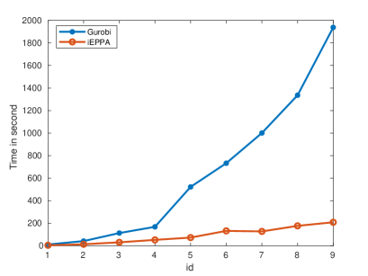
Figure 1: Comparisons between Gurobi and iEPPA for 2-marginal CMOT. In the table, “nobj” denotes the normalized objective function value, “feas” denotes the primal feasibility accuracy, “g” stands for Gurobi and “e” stands for iEPPA.

4.2 Experiments on synthetic data for 3-marginal CMOT

In this subsection, we consider the standard CMOT problem (1.2) in the 3-marginal case. Here, in view of the inferior performance of the DyKL presented in the last section, we only generate synthetic instances to evaluate the performance of our iEPPA against Gurobi to save space. Specially, we randomly generate three discrete probability distributions: $D_{1}=\left\{(a_{r},\,\bm{p}_{r})\in\mathbb{R}_{+}\times\mathbb{R}^{3}\;:\;r=1,\dots,n_{1}\right\}$, $D_{2}=\left\{(b_{s},\,\bm{q}_{s})\in\mathbb{R}_{+}\times\mathbb{R}^{3}\;:\;s=1,\dots,n_{2}\right\}$ and $D_{3}=\left\{(c_{t},\,\bm{r}_{t})\in\mathbb{R}_{+}\times\mathbb{R}^{3}\;:\;t=1,\dots,n_{3}\right\}$. Similar to the 2-marginal case in subsection 4.1, the marginals $\bm{a}:=(a_{1},\dots,a_{n_{1}})^{\top}$, $\bm{b}:=(b_{1},\dots,b_{n_{2}})^{\top}$ and $\bm{c}:=(c_{1},\dots,c_{n_{3}})^{\top}$ are all generated independently from a uniformly distribution on the interval $(0,1)$, respectively. Again, the marginals are normalized so that $\sum_{r=1}^{n_{1}}a_{r}=\sum_{s=1}^{n_{2}}b_{s}=\sum_{t=1}^{n_{3}}c_{t}=1$. Moreover, the support points are generated independently from a Gaussian mixture distribution. Given these support points, we then compute the cost tensor $C$ as follows:

$$C_{rst}:=\|\bm{p}_{r}-\bm{q}_{s}\|^{2}+\|\bm{q}_{s}-\bm{r}_{t}\|^{2}+\|\bm{r}_{t}-\bm{p}_{r}\|^{2},\quad\forall\;1\leq r\leq n_{1},~{}1\leq s\leq n_{2},~{}1\leq t\leq n_{3}.$$

We also normalize $C$ by dividing it by its maximal entry. To generate a reasonable upper bound $U$, we adapt the same strategy as in the 2-marginal case to set $U:=2\,(\bm{a}\otimes\bm{b}\otimes\bm{c})$. Figure 2 presents comparisons between iEPPA and Gurobi, where we set $n_{1}=n_{2}=n_{3}=n$ and vary $n$ from 50 to 500. Similar to the 2-marginal case in subsection 4.1.2, our iEPPA has better scalability with respect to the problem size for solving problems to a moderate accuracy.

problem		nobj		feas
id	$n$	g	e	g	e
1	50	0	4.6e-05	1.1e-12	1.0e-06
2	100	0	5.0e-05	7.0e-13	1.0e-06
3	150	0	5.0e-05	1.1e-12	9.8e-07
4	200	0	5.0e-05	1.3e-12	9.9e-07
5	250	0	4.9e-05	4.5e-13	9.9e-07
6	300	0	5.2e-05	3.2e-13	9.9e-07
7	350	0	4.9e-05	1.2e-12	9.9e-07
8	400	0	5.1e-05	1.1e-12	1.0e-06
9	450	0	5.3e-05	1.4e-12	9.9e-07
10	500	0	5.7e-05	5.3e-13	9.7e-07

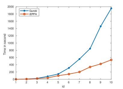
Figure 2: Comparisons between Gurobi and iEPPA for 3-marginal CMOT with $n_{1}=n_{2}=n_{3}=n$ and $n\in\{50,100,150,200,250,300,350,400,450,500\}$.

4.3 Experiments on an application to discrete tomography

In this subsection, we conduct experiments on discrete tomography to illustrate the modeling capability of our model (1.1). We should mention that the purpose here is to present a preliminary investigation on the potential of using our model together with the iEPPA+BCD framework for solving the discrete tomography problem. A thorough numerical investigation is beyond the scope of this paper and will be left as a future research topic.

Let $X$ be a 2D image of size $n\times n$ and $\vec{v}$ be a given direction that takes the form $(1,p)$, $(1,-p)$, $(p,1)$ or $(p,-1)$ with $p$ being a nonnegative integer. In our experiments, a tomographic projection on the image $X$ along $\vec{v}$ is constructed as follows: we view the image $X$ as a 2D grid of size $n\times n$, first pick all lines which are parallel to the direction $\vec{v}$ on this grid, then sum the entries on each line to form a vector. Such a projection then corresponds to a block of linear equality constraints of the form $\bm{b}^{(i)}=\mathcal{A}^{(i)}(X)$ in our model. Figure 3 shows the constructions of the tomographic projection along directions $(1,0)$ and $(2,1)$, respectively. More details on the construction can be found in Appendix C.

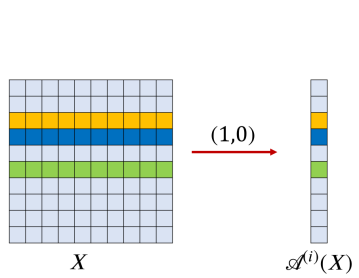
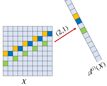
Figure 3: Examples of the operator $\mathcal{A}^{(i)}$ for direction $\vec{v}=(1,0)$ (left) and direction $\vec{v}=(2,1)$ (right).

In the following experiments, we will use five ground-truth images of size $256\times 256$ (namely, $n=256$), as shown in the first row of Figure 5. For each of them, we compute $N$ tomographic projections (which correspond to the linear mappings ${\cal A}^{(i)}$, $i=1,\dots,N$ in our model) on this image along different directions to obtain $\bm{b}^{(i)}$, $i=1,\dots,N$. Then, our goal is to recover the original image from the collection of projections $\{\bm{b}^{(i)}\}_{i=1}^{N}$ via applying our iEPPA+BCD framework for solving problem (1.1). Moreover, in our experiments, we set the entries of the cost matrix $C\in\mathbb{R}^{n\times n}$ to be $C_{rs}=|r-s|^{2}$ for $1\leq r,\,s\leq n$ and normalize $C$ by dividing (element-wise) it by its maximal entry. We do not use any upper bound matrix $U$ in the experiments. Moreover, to quantify the reconstruction quality between the recovered solution ${X}^{k}$ and the ground-truth image $X$, we evaluate the peak signal-to-noise ratio that is defined as $\mathtt{PSNR}=10\cdot\log_{10}\left(n^{2}\cdot{\max\left\{X_{rs}\,:\,1\leq r,s\leq n\right\}^{2}}/{\|{X}^{k}-X\|_{F}^{2}}\right)$.

Figure 4 presents the $\mathtt{PSNR}$ values of the reconstructed images for $N\in\{10,20,\dots,90\}$. For a better visualization, we also show the reconstructed images corresponding to $N\in\{20,50,80\}$ in Figure 5. From the results, we observe that our model (1.1) can faithfully recover the ground-truth image and the quality of the reconstructed image gradually improves when more projections are used. Thus, to improve the quality of the reconstructed image, a straightforward way is to increase the number of projections. Fortunately, for our approach of using model (1.1) and the iEPPA+BCD, imposing more projections would not increase the computational cost dramatically since the main computational unit (which is one BCD iteration) only depends on $N$ linearly. Specifically, for one more projection, we only need to add one more block of constraints in our model (1.1) and then correspondingly add one more block of dual variables in the dual BCD method.

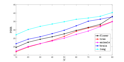
Figure 4: $\tt PSNR$ values of the reconstructed images for $N\in\{10,20,\dots,90\}$.

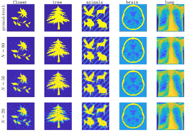
Figure 5: The first row: ground-truth images of size $256\times 256$. Here, flower, tree and animals are artificial images, while brain and chest are taken from https://radiopaedia.org/images/9219097 and https://radiopaedia.org/cases/loculated-pneumothorax, respectively. The second, third and fourth rows: reconstructed images using 80, 50 and 20 projections.

Remark 3.

To recover an $n\times n$ image by our model (1.1) (which is an LP) with $N$ available projections, the corresponding (sparse) coefficient matrix of the equality constraint has at least the size of $Nn\,\times\,n^{2}$. When $n$ and $N$ are large, such a large-scale problem can cause some LP solvers (e.g., Gurobi) to suffer from insufficient memory issues as well as high computational cost on an ordinary PC. We note that another model (based on knowing a prior distribution) that aims to recover objects from a few tomographic projections is suggested in [1, 7]. In their framework, suppose that a 2D object with $N$ projections is available. Then, the decision variable for the corresponding multi-marginal optimal transport problem will be a tensor of the order $2+N$ in the formulation given in [1]. Hence, it is difficult to implement the model efficiently. In addition, when the order of the tensor is large, the aforementioned model will invariably encounter memory issues. Moreover, our approach do not require any prior knowledge on the image to be recovered, which is another key feature that makes our modeling framework even more attractive.

5 Concluding remarks

In this paper, we propose a class of linear programming (LP) problems that can be employed to efficiently model several application problems such as discrete tomography and disaggregation of input-output tables in economics. We then develop an implementable inexact entropic proximal point algorithm (iEPPA) for solving these specially structured LPs. To solve the subproblems that contain a special entropic proximal term, we adapt an easy-to-implement dual block coordinate descent (BCD) method to solve the associated more tractable dual subproblem. The convergence of our iEPPA and the R-linear convergence of the dual BCD method are also established. In particular, we develop a new practically verifiable inexact stopping condition for solving the iEPPA subproblem that has some computational advantages over those in the existing methods. Extensive numerical experiments have been conducted to demonstrate the high efficiency and robustness of our iEPPA+BCD framework for solving the capacity constrained multi-marginal optimal transport problem. We also illustrate the potential modeling power of the proposed model by applying it to discrete tomography problems. Finally, we are aware of the classical works [30, 31] that applied the EPPA with specialized subsolvers for solving the two-stage and multi-stage stochastic network problems. It may be possible to extend our iEPPA+BCD framework for solving such special classes of LP problems. We will leave it as a future research topic.

Appendix A More details on the dual BCD

A.1 Proof of Proposition 1

First, problem (3.1) is equivalent to $\min_{X}\left\{\delta_{\Omega^{\circ}}(X)+\langle{C},\,X\rangle+\varepsilon\mathcal{D}_{\phi}(X,\,S)\right\}$. Since $\mathrm{dom}\,\phi=\mathbb{R}_{+}^{n_{1}\times n_{2}\times n_{3}}$ and thus $\Omega^{\circ}\cap\mathrm{dom}\,\phi=\Omega$ is nonempty (by Assumption 2) and bounded, then the objective function in the above problem is level bounded. Thus, a solution exists [35, Theorem 1.9] and must be unique since $\phi$ is strictly convex. The essential smoothness of $\phi$ further implies that the optimal solution can only lie in $\mathbb{R}_{++}^{n_{1}\times n_{2}\times n_{3}}$. Hence, the optimal solution of problem (3.2) also exists. Let $\big{(}\accentset{{\cc@style\underline{\mskip 10.0mu}}}{X},\,\accentset{{\cc@style\underline{\mskip 10.0mu}}}{Z}\big{)}\in\mathbb{R}^{n_{1}\times n_{2}\times n_{3}}_{++}\times\mathbb{R}^{n_{1}\times n_{2}\times n_{3}}_{++}$ be an optimal solution of problem (3.2). Since all constraint functions in (3.2) are affine and the set $\big{\{}\big{(}X,\,Z\big{)}\in\mathbb{R}^{n_{1}\times n_{2}\times n_{3}}\times\mathbb{R}^{n_{1}\times n_{2}\times n_{3}}:Z\geq 0\big{\}}$ is a convex polyhedron, then it follows from [36, Theorem 3.25] that there exist $\bar{\bm{y}}^{(i)}\in\mathbb{R}^{m_{i}},\;1\leq i\leq N$ and $\accentset{{\cc@style\underline{\mskip 10.0mu}}}{W}\in\mathbb{R}^{n_{1}\times n_{2}\times n_{3}}$ such that

$$0=M-\accentset{{\cc@style\underline{\mskip 10.0mu}}}{W}-{\textstyle\sum_{i=1}^{N}}{\cal A}^{(i,*)}\bar{\bm{y}}^{(i)}+\varepsilon\log\accentset{{\cc@style\underline{\mskip 10.0mu}}}{X},$$ (A.1)

$$0\in-\accentset{{\cc@style\underline{\mskip 10.0mu}}}{W}+\partial\delta_{+}(\accentset{{\cc@style\underline{\mskip 10.0mu}}}{Z}),$$ (A.2)

$$0=\bm{b}^{(i)}-{\cal A}^{(i)}(\accentset{{\cc@style\underline{\mskip 10.0mu}}}{X}),\quad 1\leq i\leq N,$$ (A.3)

$$0=U-\accentset{{\cc@style\underline{\mskip 10.0mu}}}{X}-\accentset{{\cc@style\underline{\mskip 10.0mu}}}{Z}.$$ (A.4)

Note from (A.1) that $\accentset{{\cc@style\underline{\mskip 10.0mu}}}{X}=\exp\Big{(}\varepsilon^{-1}\,\Big{(}{\textstyle\sum_{i=1}^{N}}{\cal A}^{(i,*)}\bar{\bm{y}}^{(i)}+\accentset{{\cc@style\underline{\mskip 10.0mu}}}{W}-M\,\Big{)}\Big{)}$. Then, substituting this and (A.4) into (A.2) and (A.3), recalling (1.4) and the fact that $\partial\delta_{+}^{*}=\partial\delta_{-}$, one can see that

$$\left\{\begin{aligned} 0&=\bm{b}^{(i)}-{\cal A}^{(i)}\Big{(}\exp\Big{(}\varepsilon^{-1}\big{(}\,{\textstyle\sum_{i=1}^{N}}{\cal A}^{(i,*)}\bar{\bm{y}}^{(i)}+\accentset{{\cc@style\underline{\mskip 10.0mu}}}{W}-M\,\big{)}\Big{)}\Big{)},\quad i=1,\dots,N,\\ 0&\in\exp\Big{(}\varepsilon^{-1}\big{(}\,{\textstyle\sum_{i=1}^{N}}{\cal A}^{(i,*)}\bar{\bm{y}}^{(i)}+\accentset{{\cc@style\underline{\mskip 10.0mu}}}{W}-M\,\big{)}\Big{)}-U+\partial\delta_{-}(\accentset{{\cc@style\underline{\mskip 10.0mu}}}{W}).\end{aligned}\right.$$ (A.5)

This together with [36, Theorem 3.5] implies that $\big{(}\bar{\bm{y}}^{(1)},\dots,\bar{\bm{y}}^{(N)},\accentset{{\cc@style\underline{\mskip 10.0mu}}}{W}\big{)}$ is an optimal solution of the dual problem (3.6) and hence the optimal solution of problem (3.6) exists.

Moreover, for any optimal solution $\big{(}\hat{\bm{y}}^{(1)},\dots,\hat{\bm{y}}^{(N)},\widehat{W}\big{)}$ of problem (3.6), it follows from [36, Theorem 3.5] that it satisfies the system (A.5) in place of $\big{(}\bar{\bm{y}}^{(1)},\dots,\bar{\bm{y}}^{(N)},\accentset{{\cc@style\underline{\mskip 10.0mu}}}{W}\big{)}$. Let $\widehat{X}:=\exp\Big{(}\varepsilon^{-1}\Big{(}\,{\textstyle\sum_{i=1}^{N}}{\cal A}^{(i,*)}\hat{\bm{y}}^{(i)}+\widehat{W}-M\,\Big{)}\Big{)}$ and $\widehat{Z}:=U-\widehat{X}$. By (1.4) and the fact that $\partial\delta_{-}^{*}=\partial\delta_{+}$, it holds that $\big{(}\widehat{X},\widehat{Z},\hat{\bm{y}}^{(1)},\dots,\hat{\bm{y}}^{(N)},\widehat{W}\big{)}$ satisfies the system (A.1)–(A.4). Thus it follows from [36, Theorem 3.27] that $\big{(}\widehat{X},\,\widehat{Z}\big{)}$ is an optimal solution of problem (3.2) and hence $\widehat{X}$ is an optimal solution of problem (3.1). This completes the proof.

A.2 Proof of Theorem 2

For the ease of applying the convergence results developed in [28], we first express problem (3.6) in the following compact form:

$$\min\limits_{\bm{\chi}}~{}\Psi(E\bm{\chi})+\langle\bm{q},\,\bm{\chi}\rangle\quad\mathrm{s.t.}\quad\bm{\chi}\in\Xi,$$ (A.6)

where $\Psi:\mathbb{R}^{n_{1}n_{2}n_{3}}\to\mathbb{R}$ is defined by $\Psi(\bm{y}):=\varepsilon\sum^{n_{1}n_{2}n_{3}}_{i}\exp((y_{i}-z_{i})/\varepsilon)$, $\bm{z}:=\mathrm{vec}(M)\in\mathbb{R}^{n_{1}n_{2}n_{3}}$, $\bm{q}:=-\big{[}\bm{b}^{(1)};\dots;\bm{b}^{(N)};\mathrm{vec}(U)\big{]}\in\mathbb{R}^{\sum_{i=1}^{N}m_{i}+n_{1}n_{2}n_{3}}$, $\bm{\chi}:=\big{[}\bm{y}^{(1)};\dots;\bm{y}^{(N)};\mathrm{vec}(W)\big{]}\in\mathbb{R}^{\sum_{i=1}^{N}m_{i}+n_{1}n_{2}n_{3}}$, $\Xi:=\big{\{}\bm{\chi}:=\big{[}\bm{y}^{(1)};\dots;\bm{y}^{(N)};\mathrm{vec}(W)\big{]}\,:\,W\leq 0\big{\}}$ and

$$E:=\big{[}\mathrm{vec}(A_{1}^{(1)}),\dots,\mathrm{vec}(A_{m_{1}}^{(1)}),\dots,\mathrm{vec}(A_{1}^{(N)}),\dots,\mathrm{vec}(A_{m_{N}}^{(N)}),I_{n_{1}n_{2}n_{3}}\big{]}\in\mathbb{R}^{n_{1}n_{2}n_{3}\times(\sum_{i=1}^{N}m_{i}+n_{1}n_{2}n_{3})}.$$

One can easily verify that $\mathrm{dom}\,\Psi=\mathbb{R}^{n_{1}n_{2}n_{3}}$ is open and $\Psi$ is strictly convex and twice continuously differentiable on $\mathrm{dom}\,\Psi$.

Moreover, the optimal solution set of problem (A.6) is nonempty (by Proposition 1) and our dual BCD in Algorithm 2 indeed falls into the algorithmic framework in [28] for solving the problem in form of (A.6). Also, note from [28, Lemma 3.3] that the set $\big{\{}E\bm{\chi}:\Psi(E\bm{\chi})+\langle\bm{q},\bm{\chi}\rangle\leq\alpha,~{}\bm{\chi}\in\Xi\big{\}}$ is compact for any $\alpha\in\mathbb{R}$. Then, one can easily verify that $\nabla^{2}\Psi(E\bm{\chi}^{*})$ is positive definite for any optimal solution $\bm{\chi}^{*}$ of problem (A.6). Based on these facts, we can readily apply [28, Theorem 2.1] to obtain statement (i), i.e., $\bm{\chi}^{t}:=(\bm{y}^{(1),t},\dots,\bm{y}^{(N),t},W^{t})\to\bm{\chi}^{*}$ R-linearly.

We next prove statement (ii). Let $\big{\{}\big{(}\hat{\bm{y}}^{(1)},\dots,\hat{\bm{y}}^{(N)},\widehat{W}\big{)}\big{\}}$ be the limit of $\big{\{}\big{(}\bm{y}^{(1),\ell},\dots,\bm{y}^{(N),\ell},W^{\ell}\big{)}\big{\}}$. Then, one can see from statement (i) that $\big{\{}\big{(}\hat{\bm{y}}^{(1)},\dots,\hat{\bm{y}}^{(N)},\widehat{W}\big{)}\big{\}}$ is an optimal solution of problem (3.6) and further see from Proposition 1 that $\widehat{X}:=\exp\big{(}\big{(}\,{\textstyle\sum_{i=1}^{N}}{\cal A}^{(i,*)}\hat{\bm{y}}^{(i)}+\widehat{W}-M\,\big{)}/\varepsilon\big{)}$ is an optimal solution of problem (3.1). Define the mapping $\mathcal{H}:\mathbb{R}^{\sum^{N}_{i=1}m_{i}+n_{1}n_{2}n_{3}}\to\mathbb{R}^{n_{1}n_{2}n_{3}}$ by $\mathcal{H}(\bm{\chi}):=\exp((E\bm{\chi}-\bm{m})/\varepsilon)$, whose Jacobian matrix is given by $\mathrm{J}\mathcal{H}(\bm{\chi})=\varepsilon^{-1}\mathrm{Diag}\big{[}\exp((E\bm{\chi}-\bm{m})/\varepsilon)\big{]}E$. Then, we see that $\bm{x}^{\ell}:=\mathrm{vec}(X^{\ell})=\mathcal{H}(\bm{\chi}^{\ell})$ and $\hat{\bm{x}}:=\mathrm{vec}(\widehat{X})=\mathcal{H}(\widehat{\bm{\chi}})$, where $\bm{\chi}^{\ell}:=\big{[}\bm{y}^{(1),\ell};\dots;\bm{y}^{(N),\ell};\mathrm{vec}(W^{\ell})\big{]}$ and $\widehat{\bm{\chi}}:=\big{[}\hat{\bm{y}}^{(1)};\dots;\hat{\bm{y}}^{(N)};\mathrm{vec}(\widehat{W})\big{]}$. Moreover, we have

$$\big{\|}\bm{x}^{\ell}-\widehat{\bm{x}}\big{\|}=\big{\|}\mathcal{H}(\bm{\chi}^{\ell})-\mathcal{H}(\widehat{\bm{\chi}})\big{\|}={\textstyle\big{\|}\big{(}\int^{1}_{0}\mathrm{J}\mathcal{H}\big{(}\widehat{\bm{\chi}}+\tau(\bm{\chi}^{\ell}-\widehat{\bm{\chi}})\big{)}\,\mathrm{d}\tau\big{)}\cdot(\bm{\chi}^{\ell}-\widehat{\bm{\chi}})\big{\|}}$$ (A.7)

$$\leq{\textstyle\big{\|}\int^{1}_{0}\mathrm{J}\mathcal{H}\big{(}\widehat{\bm{\chi}}+\tau(\bm{\chi}^{\ell}-\widehat{\bm{\chi}})\big{)}\,\mathrm{d}\tau\big{\|}\cdot\big{\|}\bm{\chi}^{\ell}-\widehat{\bm{\chi}}\big{\|}}\leq{\textstyle\int^{1}_{0}\big{\|}\mathrm{J}\mathcal{H}\big{(}\widehat{\bm{\chi}}+\tau(\bm{\chi}^{\ell}-\widehat{\bm{\chi}})\big{)}\big{\|}\,\mathrm{d}\tau\cdot\big{\|}\bm{\chi}^{\ell}-\widehat{\bm{\chi}}\big{\|}},$$

where the second equality follows from the mean-value theorem. Note that

$$\Psi(E\widehat{\bm{\chi}})+\langle\bm{q},\widehat{\bm{\chi}}\rangle\leq\Psi(E\bm{\chi}^{\ell})+\langle\bm{q},\bm{\chi}^{\ell}\rangle\leq\Psi(E\bm{\chi}^{0})+\langle\bm{q},\bm{\chi}^{0}\rangle,\quad\forall\,\ell\geq 0.$$

It then follows from [28, Lemma 3.3] that $\{E\bm{\chi}^{\ell}\}$ is bounded. With this fact, one can easily verify that $\left\|\mathrm{J}\mathcal{H}\big{(}\widehat{\bm{\chi}}+\tau(\bm{\chi}^{\ell}-\widehat{\bm{\chi}})\big{)}\right\|$ is uniformly bounded from above by some constant $L$, i.e., $\big{\|}\mathrm{J}\mathcal{H}\big{(}\widehat{\bm{\chi}}+\tau(\bm{\chi}^{\ell}-\widehat{\bm{\chi}})\big{)}\big{\|}\leq L$ for all $\ell\geq 0$ and $\tau\in[0,1]$. This together with (A.7) and statement (i) prove statement (ii).

A.3 The dual BCD for the CMOT problem

As a special case of problem (1.1), the 3-marginal capacity constrained optimal transport problem (1.2) (taking the linear mappings defined in (1.3)) has attracted particular attention. In this section, we write down the concrete iterative scheme of the dual BCD in Algorithm 2 for solving (3.1) with the constraints in (1.2). We use $\bm{f}$, $\bm{g}$, $\bm{h}$, $W$ to denote Lagrangian multipliers with respect to the following four constraints

$$\begin{array}[]{ll}{\textstyle\sum_{s,t}}X_{rst}=a_{r},~{}r=1,\dots,n_{1},&{\textstyle\sum_{r,t}}X_{rst}=b_{s},~{}s=1,\dots,n_{2},\vspace{2mm}\\ {\textstyle\sum_{r,s}}X_{rst}=c_{t},~{}t=1,\dots,n_{3},&X\leq U,\end{array}$$

respectively. By using similar arguments as in Section 3, one obtains the dual subproblem:

$$\min\limits_{\bm{f},\,\bm{g},\,\bm{h},\,W}\,R\big{(}\bm{f},\,\bm{g},\,\bm{h},\,W\big{)} :=\varepsilon\,{\textstyle\sum_{r,s,t}}\exp\big{(}\big{(}f_{r}+g_{s}+h_{t}+W_{rst}-M_{rst}\big{)}/\varepsilon\big{)}-\langle\bm{f},\,\bm{a}\rangle$$ (A.8)

$$\hskip 14.22636pt-\langle\bm{g},\,\bm{b}\rangle-\langle\bm{h},\,\bm{c}\rangle-\langle W,\,U\rangle+\delta_{-}(W),$$

where $M:=C-\varepsilon\log S$. We then apply the BCD method for solving (A.8). Specifically, start from any $(\bm{f}^{0},\bm{g}^{0},\bm{h}^{0},W^{0})\in\mathrm{dom}\,R$, at the $\ell$-th iteration, compute

$$\bm{f}^{\ell+1} =\arg\min_{\bm{f}}\,R\big{(}\bm{f},\,\bm{g}^{\ell},\,\bm{h}^{\ell},\,W^{\ell}\big{)},\quad\quad\quad\;\bm{g}^{\ell+1}=\arg\min_{\bm{g}}\,R\big{(}\bm{f}^{\ell+1},\,\bm{g},\,\bm{h}^{\ell},\,W^{\ell}\big{)},$$

$$\bm{h}^{\ell+1} =\arg\min_{\bm{h}}\,R\big{(}\bm{f}^{\ell+1},\,\bm{g}^{\ell+1},\,\bm{h},\,W^{\ell}\big{)},\quad W^{\ell+1}=\arg\min_{W}\,R\big{(}\bm{f}^{\ell+1},\,\bm{g}^{\ell+1},\,\bm{h}^{\ell+1},\,W\big{)}.$$

After some manipulations, one can obtain the following explicit iterative scheme:

$$\bm{f}^{\ell+1} =\varepsilon\log(\bm{a})-\varepsilon\log\left(\left[{\textstyle\sum_{s,t}}\exp\big{(}\big{(}g_{s}^{\ell}+h_{t}^{\ell}+W_{rst}^{\ell}-M_{rst}\big{)}/\varepsilon\big{)}\right]_{r=1}^{n_{1}}\right),$$ (A.9)

$$\bm{g}^{\ell+1} =\varepsilon\log(\bm{b})-\varepsilon\log\left(\left[{\textstyle\sum_{r,t}}\exp\left(\big{(}f_{r}^{\ell+1}+h_{t}^{\ell}+W_{rst}^{\ell}-M_{rst}\big{)}/\varepsilon\right)\right]_{s=1}^{n_{2}}\right),$$

$$\bm{h}^{\ell+1} =\varepsilon\log(\bm{c})-\varepsilon\log\left(\left[{\textstyle\sum_{r,s}}\exp\big{(}\big{(}f_{r}^{\ell+1}+g_{s}^{\ell+1}+W_{rst}^{\ell}-M_{rst}\big{)}/\varepsilon\big{)}\right]_{t=1}^{n_{3}}\right),$$

$$W^{\ell+1} =\min\left\{\varepsilon\log U+M-\bm{f}^{\ell+1}\otimes\bm{1}_{n_{2}}\otimes\bm{1}_{n_{3}}-\bm{1}_{n_{1}}\otimes\bm{g}^{\ell+1}\otimes\bm{1}_{n_{3}}-\bm{1}_{n_{1}}\otimes\bm{1}_{n_{2}}\otimes\bm{h}^{\ell+1},\,0\right\},$$

where $\bm{1}_{n_{i}}$ denotes the $n_{i}$-dimensional vector of all ones for $i=1,\,2,\,3$. Moreover, let $\widetilde{M}:=\exp(-{M/\varepsilon})$, $\tilde{\bm{f}}^{\ell}:=\exp({\bm{f}^{\ell}/\varepsilon})$, $\tilde{\bm{g}}^{\ell}:=\exp({\bm{g}^{\ell}/\varepsilon})$, $\tilde{\bm{h}}^{\ell}:=\exp({\bm{h}^{\ell}/\varepsilon})$ and $\widetilde{W}^{\ell}:=\exp({W^{\ell}/\varepsilon})$. Then, we can equivalently rewrite the iterative scheme (A.9) as

$$\tilde{\bm{f}}^{\ell+1} =\bm{a}\,.\Big{/}\Big{(}\Big{[}\sum_{s,t}(\widetilde{W}^{\ell}\circ\widetilde{M}\big{)}_{rst}\,\tilde{g}_{s}^{\ell}\,\tilde{h}_{t}^{\ell}\Big{]}_{r=1}^{n_{1}}\Big{)},\quad\,\,\tilde{\bm{g}}^{\ell+1}=\bm{b}\,.\Big{/}\Big{(}\Big{[}\sum_{r,t}(\widetilde{W}^{\ell}\circ\widetilde{M}\big{)}_{rst}\,\tilde{f}_{r}^{\ell+1}\,\tilde{h}_{t}^{\ell}\Big{]}_{s=1}^{n_{2}}\Big{)},$$ (A.10)

$$\tilde{\bm{h}}^{\ell+1} =\bm{c}\,.\Big{/}\Big{(}\Big{[}\sum_{r,s}(\widetilde{W}^{\ell}\circ\widetilde{M}\big{)}_{rst}\,\tilde{f}_{r}^{\ell+1}\,\tilde{g}_{s}^{\ell+1}\Big{]}_{t=1}^{n_{3}}\Big{)},\quad\widetilde{W}^{\ell+1}=\min\Big{\{}\big{(}U./\widetilde{M}\big{)}\,.\big{/}\big{(}\tilde{\bm{f}}^{\ell+1}\otimes\tilde{\bm{g}}^{\ell+1}\otimes\tilde{\bm{h}}^{\ell+1}\big{)},\,1\Big{\}}.$$

In our numerical experiments conducted in Section 4, we always adopt the iterative scheme (A.10) since the proximal parameter $\varepsilon$ in our iEPPA does not need to take a small value.

Appendix B Dykstra’s algorithm with KL projections

Dykstra’s algorithm with Kullback-Leibler projections (DyKL) [5] is adapted in [6] to solve the following entropic regularized capacity constrained optimal transport problem:

$$\min\limits_{X\in\mathbb{R}^{m\times n}}\,\langle C,\,X\rangle+\varepsilon{\textstyle\sum^{m}_{s=1}\sum^{n}_{r=1}}X_{rs}(\log X_{rs}-1)$$ (B.1)

$$\hskip 12.80365pt\mathrm{s.t.}\hskip 14.22636ptX\bm{1}_{n}=\bm{a},~{}~{}X^{\top}\bm{1}_{m}=\bm{b},~{}~{}0\leq X\leq U,$$

where $C\in\mathbb{R}^{m\times n}_{+}$, $U\in\mathbb{R}^{m\times n}_{++}$, $\bm{a}:=(a_{1},\dots,a_{m})^{\top}\in\Sigma_{m}$, $\bm{b}:=(b_{1},\dots,b_{n})^{\top}\in\Sigma_{n}$. Recall the definition of the Kullback-Leibler (KL) divergence between $X\in\mathbb{R}^{m\times n}_{+}$ and $Y\in\mathbb{R}^{m\times n}_{++}$ is given as follows:

$$\mathbf{KL}(X,\,Y)={\textstyle\sum_{r,s}}\left(x_{rs}\log\left(x_{rs}/y_{rs}\right)-x_{rs}+y_{rs}\right).$$

Moreover, given a convex set $\mathcal{S}\subseteq\mathbb{R}^{m\times n}$ and $Y\in\mathbb{R}^{m\times n}_{++}$, the projection associated with the KL divergence (called KL projection) is defined as $\mathrm{Proj}^{\mathbf{KL}}_{\mathcal{S}}(Y):=\arg\min\limits_{X\in\mathcal{S}}~{}\mathbf{KL}(X,\,Y)$. Thus, problem (B.1) can be equivalently reformulated as

$$\min_{X\in\mathbb{R}^{m\times n}}~{}\mathbf{KL}(X,\,K)\qquad\mathrm{s.t.}\qquad X\in\mathcal{S}_{1}\cap\mathcal{S}_{2}\cap\mathcal{S}_{3},$$

where $K:=e^{-C/\varepsilon}$ is the kernel matrix, $\mathcal{S}_{1}:=\{X\in\mathbb{R}^{m\times n}\,:\,X\bm{1}_{n}=\bm{a}\}$, $\mathcal{S}_{2}:=\{X\in\mathbb{R}^{m\times n}\,:\,X^{\top}\bm{1}_{m}=\bm{b}\}$ and $\mathcal{S}_{3}:=\{X\in\mathbb{R}^{m\times n}\,:\,X\leq U\}$. Then, the DyKL is presented as follows: let $X^{0}=K$, $Q^{0}_{1}=Q^{0}_{2}=Q^{0}_{3}=\bm{1}_{m}\bm{1}_{n}^{\top}$, then for $k\geq 0$, compute

$$\Pi^{k+1}_{0} =X^{k},$$ (B.2)

$$\Pi^{k+1}_{1} =\mathrm{Proj}^{\mathbf{KL}}_{\mathcal{S}_{1}}(\Pi^{k+1}_{0}\circ Q^{k}_{1}),~{}~{}Q^{k+1}_{1}=Q^{k}_{1}\circ\big{(}\Pi^{k+1}_{0}./\Pi^{k+1}_{1}\big{)},$$

$$\Pi^{k+1}_{2} =\mathrm{Proj}^{\mathbf{KL}}_{\mathcal{S}_{2}}(\Pi^{k+1}_{1}\circ Q^{k}_{2}),~{}~{}Q^{k+1}_{2}=Q^{k}_{2}\circ\big{(}\Pi^{k+1}_{1}./\Pi^{k+1}_{2}\big{)},$$

$$\Pi^{k+1}_{3} =\mathrm{Proj}^{\mathbf{KL}}_{\mathcal{S}_{3}}(\Pi^{k+1}_{2}\circ Q^{k}_{3}),~{}~{}Q^{k+1}_{3}=Q^{k}_{3}\circ\big{(}\Pi^{k+1}_{2}./\Pi^{k+1}_{3}\big{)},$$

$$X^{k+1} =\Pi^{k+1}_{3},$$

where $\circ$ denotes the Hadamard product. Note that the above iterative scheme is a slightly different but an equivalent form of the DyKL used in [6]. We adapt it here because it is more explicit and convenient for comparison. Moreover, by simple calculations, one can verify that

$$\Pi^{k+1}_{1} =\mathrm{Proj}^{\mathbf{KL}}_{\mathcal{S}_{1}}(\Pi^{k+1}_{0}\circ Q^{k}_{1})=\mathrm{Diag}\Big{(}\bm{a}.\big{/}\big{(}\big{(}\Pi^{k+1}_{0}\circ Q^{k}_{1}\big{)}\bm{1}_{n}\big{)}\Big{)}\,\big{(}\Pi^{k+1}_{0}\circ Q^{k}_{1}\big{)},$$

$$\Pi^{k+1}_{2} =\mathrm{Proj}^{\mathbf{KL}}_{\mathcal{S}_{2}}(\Pi^{k+1}_{1}\circ Q^{k}_{2})=\big{(}\Pi^{k+1}_{1}\circ Q^{k}_{2}\big{)}\,\mathrm{Diag}\Big{(}\bm{b}.\big{/}\big{(}\big{(}\Pi^{k+1}_{1}\circ Q^{k}_{2}\big{)}^{\top}\bm{1}_{m}\big{)}\Big{)},$$

$$\Pi^{k+1}_{3} =\mathrm{Proj}^{\mathbf{KL}}_{\mathcal{S}_{3}}(\Pi^{k+1}_{2}\circ Q^{k}_{3})=\min\big{\{}\Pi^{k+1}_{2}\circ Q^{k}_{3},\,U\big{\}}.$$

It is worth noting that the DyKL in (B.2) may suffer from severe numerical issues when $\varepsilon$ takes a small value. Thus, one may need to carry out the computations of $\Pi^{k}_{i}$ and $Q^{k}_{i}$ ($i=1,2,3$) in the log domain to alleviate the numerical instability. Specifically, by taking logarithm on both sides of above equations and letting $\widetilde{X}^{k}:=\varepsilon\log X^{k}$, $\widetilde{\Pi}^{k}_{i}:=\varepsilon\log\Pi^{k}_{i}$, $\widetilde{Q}^{k}_{i}:=\varepsilon\log Q^{k}_{i}$, $\tilde{\bm{a}}:=\varepsilon\log\bm{a}$, $\widetilde{U}:=\varepsilon\log U$, we obtain after some manipulations that

$$\begin{array}[]{llll}\widetilde{\Pi}^{k+1}_{0}=\widetilde{X}^{k},\\[5.0pt] \widetilde{\Pi}^{k+1}_{1}=\left[\tilde{\bm{a}}-\varepsilon\log\left(\left[\exp\big{(}\big{(}\widetilde{\Pi}^{k+1}_{0}+\widetilde{Q}^{k}_{1}\big{)}/\varepsilon\big{)}\right]\bm{1}_{n}\right)\right]\bm{1}_{n}^{\top}+\widetilde{\Pi}^{k+1}_{0}+\widetilde{Q}^{k}_{1},&\widetilde{Q}^{k+1}_{1}=\widetilde{Q}^{k}_{1}+\widetilde{\Pi}^{k+1}_{0}-\widetilde{\Pi}^{k+1}_{1},\\[5.0pt] \widetilde{\Pi}^{k+1}_{2}=\bm{1}_{m}\left[\tilde{\bm{b}}-\varepsilon\log\left(\left[\exp\big{(}\big{(}\widetilde{\Pi}^{k+1}_{1}+\widetilde{Q}^{k}_{2}\big{)}/\varepsilon\big{)}\right]^{\top}\bm{1}_{m}\right)\right]^{\top}+\widetilde{\Pi}^{k+1}_{1}+\widetilde{Q}^{k}_{2},&\widetilde{Q}^{k+1}_{2}=\widetilde{Q}^{k}_{2}+\widetilde{\Pi}^{k+1}_{1}-\widetilde{\Pi}^{k+1}_{2},\\[5.0pt] \widetilde{\Pi}^{k+1}_{3}=\min\big{\{}\widetilde{\Pi}^{k+1}_{2}+\widetilde{Q}^{k}_{3},\,\widetilde{U}\big{\}},&\widetilde{Q}^{k+1}_{3}=\widetilde{Q}^{k}_{3}+\widetilde{\Pi}^{k+1}_{2}-\widetilde{\Pi}^{k+1}_{3},\\[5.0pt] \widetilde{X}^{k+1}=\widetilde{\Pi}^{k+1}_{3}.\end{array}$$ (B.3)

In this stabilization framework, the initialization is set to $\widetilde{X}^{0}=-C$ and $\widetilde{Q}^{0}_{1}=\widetilde{Q}^{0}_{2}=\widetilde{Q}^{0}_{3}=0$. When checking the primal feasibility accuracy, we recover $X^{k+1}$ by setting $X^{k+1}=\exp(\widetilde{X}^{k+1}/\varepsilon)$.

Appendix C Construction of a tomographic projection

Let $p$ be a nonnegative integer. We consider the following four directions

$$\vec{v}=(1,\,p),~{}(1,\,-p),~{}(p,1)~{}\textrm{and}~{}(p,\,-1).$$

Note that when $p\in\{0,1\}$, we only have two directions. The process to find the projection ${\cal A}^{(i)}(X)$ along a given direction $\vec{v}$ is described as follows (see Figure 6 for a concrete example):

• Plot the entries of $X$ as points on the integer grid $\{1,\ldots,n\}\times\{1,\ldots,n\}$.

• For each point, draw a line $\mathsf{v}_{j}$ parallelling to $\vec{v}$, identify all other points for which $\mathsf{v}_{j}$ passes through.

• Take the sum of the entries of $X$ for all points on $\mathsf{v}_{j}$ to define $({\cal A}^{(i)}(X))_{j}$.

• Repeat this process until all $\{\mathsf{v}_{j}\}$ covers the whole grid, i.e., covers all entries of $X$.

Figure 6: Construction of the projection operator along $\vec{v}=(2,1)$ for a $5\times 5$ matrix $X$.

Declarations

Data availability Not applicable.

References

- [1] I. Abraham, R. Abraham, M. Bergounioux, and G. Carlier. Tomographic reconstruction from a few views: A multi-marginal optimal transport approach. Appl. Math. Optim., 75(1):55–73, 2017.
- [2] J. Altschuler, J. Weed, and P. Rigollet. Near-linear time approximation algorithms for optimal transport via Sinkhorn iteration. In Advances in Neural Information Processing Systems, volume 30, 2017.
- [3] A. Auslender and M. Haddou. An interior-proximal method for convex linearly constrained problems and its extension to variational inequalities. Math. Program., 71(1):77–100, 1995.
- [4] H.H. Bauschke and J.M. Borwein. Legendre functions and the method of random Bregman projections. J. Convex Anal., 4(1):27–67, 1997.
- [5] H.H. Bauschke and A.S. Lewis. Dykstras algorithm with Bregman projections: A convergence proof. Optimization, 48(4):409–427, 2000.
- [6] J.-D. Benamou, G. Carlier, M. Cuturi, L. Nenna, and G. Peyré. Iterative Bregman projections for regularized transportation problems. SIAM J. Sci. Comput., 37(2):A1111–A1138, 2015.
- [7] M. Bergounioux, I. Abraham, R. Abraham, G. Carlier, E. Le Pennec, and E. Trélat. Variational methods for tomographic reconstruction with few views. Milan J. Math., 86(2):157–200, 2018.
- [8] D. Bertsimas and J.N. Tsitsiklis. Introduction to Linear Optimization. Athena Scientific Belmont, MA, 1997.
- [9] L.M. Bregman. The relaxation method of finding the common point of convex sets and its application to the solution of problems in convex programming. USSR Comput. Math. Math. Phys., 7(3):200–217, 1967.
- [10] Y. Censor and A. Lent. An iterative row-action method for interval convex programming. J. Optim. Theory Appl., 34(3):321–353, 1981.
- [11] Y. Censor and S.A. Zenios. Proximal minimization algorithm with -functions. J. Optim. Theory Appl., 73(3):451–464, 1992.
- [12] G. Chen and M. Teboulle. Convergence analysis of a proximal-like minimization algorithm using Bregman functions. SIAM J. Optim., 3(3):538–543, 1993.
- [13] M. Cuturi. Sinkhorn distances: Lightspeed computation of optimal transport. In Advances in Neural Information Processing Systems, pages 2292–2300, 2013.
- [14] R.L. Dykstra. An algorithm for restricted least squares regression. J. Am. Stat. Assoc., 78(384):837–842, 1983.
- [15] J. Eckstein. Nonlinear proximal point algorithms using Bregman functions, with applications to convex programming. Math. Oper. Res., 18(1):202–226, 1993.
- [16] J. Eckstein. Approximate iterations in Bregman-function-based proximal algorithms. Math. Prog., 83(1-3):113–123, 1998.
- [17] P.P.B Eggermont. Multiplicative iterative algorithms for convex programming. Linear Algebra Appl., 130:25–42, 1990.
- [18] A. Grandy and L. Veraart. Bayesian methodology for systemic risk assessment in financial networks. Manage. Sci., 63:3999–4446, 2017.
- [19] A.J. Hoffman. On approximate solutions of systems of linear inequalities. J. Res. Natl. Bur. Stand., 49(4):263–265, 1952.
- [20] V. Holy and K. Safr. Disaggregating input-output tables by the multidimensional RAS method. arXiv preprint arXiv:1704.078142v2, 2019.
- [21] A.N. Iusem, B.F. Svaiter, and M. Teboulle. Entropy-like proximal methods in convex programming. Math. Oper. Res., 19(4):790–814, 1994.
- [22] A.N. Iusem and M. Teboulle. Convergence rate analysis of nonquadratic proximal methods for convex and linear programming. Math. Oper. Res., 20(3):657–677, 1995.
- [23] J. Kennington and M. Shalaby. An effective subgradient procedure for minimal cost multicommodity flow problems. Manage. Sci., 23(9):994–1004, 1977.
- [24] J. Korman and R.J. McCann. Insights into capacity-constrained optimal transport. Proc. Natl. Acad. Sci., 110(25):10064–10067, 2013.
- [25] J. Korman and R.J. McCann. Optimal transportation with capacity constraints. Trans. Am. Math. Soc., 367(3):1501–1521, 2015.
- [26] V.L. Levin. The problem of mass transfer in a topological space and probability measures with given marginal measures on the product of two spaces. Dokl. Akad. Nauk SSSR, 276(5):1059–1064, 1984.
- [27] T. Lin, N. Ho, M. Cuturi, and M.I. Jordan. On the complexity of approximating multimarginal optimal transport. To appear in J. Mach. Learn. Res., 2022.
- [28] Z.-Q. Luo and P. Tseng. On the convergence of the coordinate descent method for convex differentiable minimization. J. Optim. Theory Appl., 72(1):7–35, 1992.
- [29] Z.-Q. Luo and P. Tseng. On the convergence rate of dual ascent methods for linearly constrained convex minimization. Math. Oper. Res., 18(4):846–867, 1993.
- [30] S. S Nielsen and S. A Zenios. Massively parallel proximal algorithms for solving linear stochastic network programs. The Int. J. Supercomput Appl., 7(4):349–364, 1993.
- [31] S. S Nielsen and S. A Zenios. Solving multistage stochastic network programs on massively parallel computers. Math. Program., 73(3):227–250, 1996.
- [32] G. Peyré and M. Cuturi. Computational optimal transport. Found. Trends Mach. Learn., 11(5-6):355–607, 2019.
- [33] B. T. Polyak. Introduction to optimization. Optimization Software Inc., New York, 1987.
- [34] R. T. Rockafellar. Convex Analysis. Princeton University Press, Princeton, 1970.
- [35] R. T. Rockafellar and R. J-B. Wets. Variational Analysis. Springer, 1998.
- [36] A. Ruszczyński. Nonlinear Optimization. Princeton University Press, Princeton, 2006.
- [37] R. Sinkhorn. Diagonal equivalence to matrices with prescribed row and column sums. Am. Math. Mon., 74(4):402–405, 1967.
- [38] M. Teboulle. Entropic proximal mappings with applications to nonlinear programming. Math. Oper. Res., 17(3):670–690, 1992.
- [39] M. Teboulle. Convergence of proximal-like algorithms. SIAM J. Optim., 7(4):1069–1083, 1997.
- [40] R.J. Tibshirani. Dykstra’s algorithm, ADMM, and coordinate descent: Connections, insights, and extensions. In Advances in Neural Information Processing Systems, pages 517–528, 2017.
- [41] P. Tseng. Dual coordinate ascent methods for non-strictly convex minimization. Math. Program., 59(1-3):231–247, 1993.
- [42] S. Weber, C. Schnörr, T. Schüle, and J. Hornegger. Binary tomography by iterating linear programs. In Geometric Properties for Incomplete Data, pages 183–197, 2006.
- [43] Y. Xie, X. Wang, R. Wang, and H. Zha. A fast proximal point method for computing exact Wasserstein distance. In Proceedings of the 35th Uncertainty in Artificial Intelligence Conference, pages 433–453, 2020.