Prediction of hidden-charm pentaquarks with double strangeness

Abstract

Inspired by the recent evidence of $P_{cs}(4459)$ reported by LHCb, we continue to perform the investigation of hidden-charm molecular pentaquarks with double strangeness, which are composed of an $S$-wave charmed baryon $\Xi_{c}^{(\prime,*)}$ and an $S$-wave anti-charmed-strange meson $\bar{D}_{s}^{(*)}$. Both the $S$-$D$ wave mixing effect and the coupled channel effect are taken into account in realistic calculation. A dynamics calculation shows that there may exist two types of hidden-charm molecular pentaquark with double strangeness, i.e., the $\Xi_{c}^{*}\bar{D}_{s}^{*}$ molecular state with $J^{P}={5}/{2}^{-}$ and the $\Xi_{c}^{\prime}\bar{D}_{s}^{*}$ molecular state with $J^{P}={3}/{2}^{-}$. According to this result, we strongly suggest the experimental exploration of hidden-charm molecular pentaquarks with double strangeness. Facing such opportunity, obviously the LHCb will have great potential to hunt for them, with the data accumulation at Run III and after High-Luminosity-LHC upgrade.

I Introduction

Very recently, the LHCb Collaboration reported the evidence of a possible hidden-charm pentaquark with strangeness $P_{cs}(4459)$ by analyzing the $\Xi_{b}^{-}\to J/\psi K^{-}\Lambda$ process, where this enhancement structure existing in the $J/\psi\Lambda$ invariant mass spectrum has the mass $4458.8\pm 2.9^{+4.7}_{-1.1}$ MeV and the width $17.3\pm 6.5^{+8.0}_{-5.7}$ MeV lhcb . In fact, before this announcement, several theoretical groups Chen:2016ryt ; Wu:2010vk ; Hofmann:2005sw ; Anisovich:2015zqa ; Wang:2015wsa ; Feijoo:2015kts ; Lu:2016roh ; Xiao:2019gjd ; Shen:2020gpw ; Chen:2015sxa ; Zhang:2020cdi ; Wang:2019nvm predicted the existence of hidden-charm pentaquarks with strangeness and suggested experimentalist to carry out the search for them. After reporting $P_{cs}(4459)$, there were also theoretical studies to decode $P_{cs}(4459)$, where $P_{cs}(4459)$ can be assigned as the $\Xi_{c}\bar{D}^{*}$ molecular state Chen:2020uif ; Peng:2020hql ; 1830432 ; 1830426 ; 1830449 .

In fact, the above experimental investigation of pentaquark is a continuation of the past. In 2015, the LHCb Collaboration released the observation of $P_{c}(4380)$ and $P_{c}(4450)$ in the $J/\psi p$ invariant mass spectrum of the $\Lambda_{b}\to J/\psi pK$ process Aaij:2015tga . In 2019, based on more collected data, the LHCb Collaboration again analyzed the same process and found a new $P_{c}(4312)$ and indicated that $P_{c}(4450)$ contains two substructures $P_{c}(4440)$ and $P_{c}(4457)$ Aaij:2019vzc , which may provide strong evidence of hidden-charm molecular pentaquarks existing in nature Li:2014gra ; Karliner:2015ina ; Wu:2010jy ; Wang:2011rga ; Yang:2011wz ; Wu:2012md ; Chen:2015loa .

When facing such new progress on exploring hidden-charm pentaquarks Chen:2016qju ; Liu:2019zoy ; Olsen:2017bmm ; Guo:2017jvc , we naturally expect that there should form a zoo of hidden-charm pentaquarks which is composed of different kinds of hidden-charm pentaquarks (see Fig. 1). If considering the difference of strangeness in hidden-charm pentaquarks, we want to further get the information of hidden-charm pentaquarks with double strangeness $|S|=2$ when $P_{cs}(4459)$ with strangeness $|S|=1$ was announced, which will be the main task of this work.

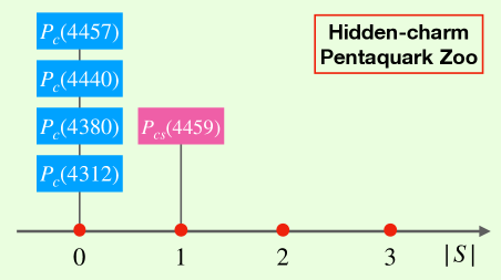
Figure 1: The hidden-charm pentaquark zoo with different values of strangeness.

In this work, we study hadronic molecular states composed of an $S$-wave charmed baryon $\Xi_{c}^{(\prime,*)}$ and an $S$-wave anti-charmed-strange meson $\bar{D}_{s}^{(*)}$. Here, $\Xi_{c}$ with $J^{P}=1/2^{+}$ denotes $S$-wave charmed baryon in $\bar{3}_{F}$ flavor representation, while $S$-wave charmed baryons $\Xi_{c}^{\prime}$ with $J^{P}=1/2^{+}$ and $\Xi_{c}^{*}$ with $J^{P}=3/2^{+}$ are in $6_{F}$ flavor representation. For obtaining the effective potentials of these discussed systems, we adopt the one-boson-exchange (OBE) model. With the extracted effective potentials, we may find the bound state solutions of the discussed systems, and further conclude whether there exist possible hidden-charm molecular pentaquarks with double strangeness. By this effort, we may give theoretical suggestion of performing the search for them in experiment.

For Large Hadron Collider (LHC), Run III will be carried out in near future. After that, the High-Luminosity-LHC upgrade will eventually collect an integrated luminosity of 300 $\rm{fb^{-1}}$ of data in pp collisions at a centre-of-mass energy of 14 TeV Bediaga:2018lhg . Thus, we have reason to believe that exploring these suggested hidden-charm molecular pentaquarks with double strangeness will be an interesting research issue full of opportunity, especially at the LHCb.

This paper is organized as the follows. After introduction, the detailed calculation of the interactions of these discussed $\Xi_{c}^{(\prime,*)}\bar{D}_{s}^{(*)}$ systems will be given in Sec. II. With this preparation, we present the bound state properties for these possible hidden-charm pentaquark molecules with double strangeness in Sec. III. Finally, this work ends with a short summary in Sec. IV.

II Effective potentials of the $\Xi_{c}^{(\prime,*)}\bar{D}_{s}^{(*)}$ systems

In this work, we mainly study the interactions between an $S$-wave charmed baryon $\Xi_{c}^{(\prime,*)}$ and an $S$-wave anti-charmed-strange meson $\bar{D}_{s}^{(*)}$ in the OBE model, we include the contribution from the pseudoscalar meson, scalar meson, and vector meson exchanges in our concrete calculation, which is often adopted to study the hadron interactions Chen:2016qju ; Liu:2019zoy .

II.1 Deducing the effective potentials

As shown in Refs. Wang:2020dya ; Wang:2019nwt , there usually exist three typical steps for calculating the effective potentials of these discussed $\Xi_{c}^{(\prime,*)}\bar{D}_{s}^{(*)}$ systems, we will give a brief introduction in the following.

Firstly, we can obtain the scattering amplitudes $\mathcal{M}(h_{1}h_{2}\to h_{3}h_{4})$ for the $h_{1}h_{2}\to h_{3}h_{4}$ processes with the effective Lagrangian approach. Here, we need to construct the relevant effective Lagrangians in the present work.

If considering the heavy quark symmetry, chiral symmetry Wise:1992hn ; Casalbuoni:1992gi ; Casalbuoni:1996pg ; Yan:1992gz , and hidden local symmetry Bando:1987br ; Harada:2003jx , the effective Lagrangians for depicting the heavy hadrons $\bar{D}_{s}^{(*)}/\mathcal{B}_{c}^{(*)}$ coupling with the light scalar, pesudoscalar, and vector mesons read as Ding:2008gr ; Chen:2017xat

$$\mathcal{L}_{H} = g_{S}\langle\bar{H}^{(\overline{Q})}_{a}\sigma H^{(\overline{Q})}_{b}\rangle+ig\langle\bar{H}^{(\overline{Q})}_{a}\gamma_{\mu}{\mathcal{A}}_{ab}^{\mu}\gamma_{5}H^{(\overline{Q})}_{b}\rangle$$

$$-i\beta\langle\bar{H}^{(\overline{Q})}_{a}v_{\mu}\left(\mathcal{V}^{\mu}-\rho^{\mu}\right)_{ab}H^{(\overline{Q})}_{b}\rangle$$

$$+i\lambda\langle\bar{H}^{(\overline{Q})}_{a}\sigma_{\mu\nu}F^{\mu\nu}(\rho)H^{(\overline{Q})}_{b}\rangle,$$

$$\mathcal{L}_{\mathcal{B}_{\bar{3}}} = l_{B}\langle\bar{\mathcal{B}}_{\bar{3}}\sigma\mathcal{B}_{\bar{3}}\rangle+i\beta_{B}\langle\bar{\mathcal{B}}_{\bar{3}}v^{\mu}(\mathcal{V}_{\mu}-\rho_{\mu})\mathcal{B}_{\bar{3}}\rangle,$$

$$\mathcal{L}_{\mathcal{B}^{(*)}_{6}} = l_{S}\langle\bar{\mathcal{S}}_{\mu}\sigma\mathcal{S}^{\mu}\rangle-\frac{3}{2}g_{1}\varepsilon^{\mu\nu\lambda\kappa}v_{\kappa}\langle\bar{\mathcal{S}}_{\mu}{\mathcal{A}}_{\nu}\mathcal{S}_{\lambda}\rangle$$

$$+i\beta_{S}\langle\bar{\mathcal{S}}_{\mu}v_{\alpha}\left(\mathcal{V}^{\alpha}-\rho^{\alpha}\right)\mathcal{S}^{\mu}\rangle+\lambda_{S}\langle\bar{\mathcal{S}}_{\mu}F^{\mu\nu}(\rho)\mathcal{S}_{\nu}\rangle,$$

$$\mathcal{L}_{\mathcal{B}_{\bar{3}}\mathcal{B}^{(*)}_{6}} = ig_{4}\langle\bar{\mathcal{S}^{\mu}}{\mathcal{A}}_{\mu}\mathcal{B}_{\bar{3}}\rangle+i\lambda_{I}\varepsilon^{\mu\nu\lambda\kappa}v_{\mu}\langle\bar{\mathcal{S}}_{\nu}F_{\lambda\kappa}\mathcal{B}_{\bar{3}}\rangle+h.c..$$ (2.1)

Here, $v=(1,\bm{0})$ is the four velocity under the non-relativistic approximation. The super-field $H^{(\overline{Q})}_{a}$ is given by $H^{(\overline{Q})}_{a}=\left(\bar{D}^{*(\overline{Q})\mu}_{a}\gamma_{\mu}-\bar{D}^{(\overline{Q})}_{a}\gamma_{5}\right)\frac{1-/\!\!\!v}{2}$, which is expressed as a combination of the vector anti-charmed-strange meson $\bar{D}^{*}_{s}$ with $J^{P}=1^{-}$ and the pseudoscalar anti-charmed-strange meson $\bar{D}_{s}$ with $J^{P}=0^{-}$. And the super-field $\mathcal{S}_{\mu}$ can be written as $\mathcal{S}_{\mu}=-\sqrt{\frac{1}{3}}(\gamma_{\mu}+v_{\mu})\gamma^{5}\mathcal{B}_{6}+\mathcal{B}_{6\mu}^{*}$, which includes the charmed baryons $\mathcal{B}_{6}$ with $J^{P}=1/2^{+}$ and $\mathcal{B}^{*}_{6}$ with $J^{P}=3/2^{+}$ in the $6_{F}$ flavor representation. Matrices $\mathcal{B}_{\bar{3}}$ and $\mathcal{B}_{6}^{(*)}$ are given by

$$\mathcal{B}_{\bar{3}}=\left(\begin{array}[]{ccc}0&\Lambda_{c}^{+}&\Xi_{c}^{+}\\ -\Lambda_{c}^{+}&0&\Xi_{c}^{0}\\ -\Xi_{c}^{+}&-\Xi_{c}^{0}&0\end{array}\right),\mathcal{B}_{6}^{(*)}=\left(\begin{array}[]{ccc}\Sigma_{c}^{{(*)}++}&\frac{\Sigma_{c}^{{(*)}+}}{\sqrt{2}}&\frac{\Xi_{c}^{(^{\prime},*)+}}{\sqrt{2}}\\ \frac{\Sigma_{c}^{{(*)}+}}{\sqrt{2}}&\Sigma_{c}^{{(*)}0}&\frac{\Xi_{c}^{(^{\prime},*)0}}{\sqrt{2}}\\ \frac{\Xi_{c}^{(^{\prime},*)+}}{\sqrt{2}}&\frac{\Xi_{c}^{(^{\prime},*)0}}{\sqrt{2}}&\Omega_{c}^{(*)0}\end{array}\right),$$ (2.8)

respectively. In addition, the axial current $\mathcal{A}_{\mu}$, the vector current ${\cal V}_{\mu}$, the vector meson field $\rho_{\mu}$, and the vector meson strength tensor $F_{\mu\nu}(\rho)$ are defined as

$${\mathcal{A}}_{\mu} = \frac{1}{2}\left(\xi^{\dagger}\partial_{\mu}\xi-\xi\partial_{\mu}\xi^{\dagger}\right)_{\mu},$$

$${\mathcal{V}}_{\mu} = \frac{1}{2}\left(\xi^{\dagger}\partial_{\mu}\xi+\xi\partial_{\mu}\xi^{\dagger}\right)_{\mu},$$

$$\rho_{\mu} = \frac{i{g_{V}}}{{\sqrt{2}}}\mathbb{V}_{\mu},$$

$$F_{\mu\nu}(\rho) = \partial_{\mu}\rho_{\nu}-\partial_{\nu}\rho_{\mu}+\left[\rho_{\mu},\rho_{\nu}\right],$$ (2.9)

respectively. Here, $\xi=\exp(i\mathbb{P}/f_{\pi})$ with $f_{\pi}$ as the pion decay constant, ${\mathbb{P}}$ and $\mathbb{V}_{\mu}$ correspond to the light pseudoscalar and vector meson matrices, which are expressed as

$$\left.\begin{array}[]{c}{\mathbb{P}}={\left(\begin{array}[]{ccc}\frac{\pi^{0}}{\sqrt{2}}+\frac{\eta}{\sqrt{6}}&\pi^{+}&K^{+}\\ \pi^{-}&-\frac{\pi^{0}}{\sqrt{2}}+\frac{\eta}{\sqrt{6}}&K^{0}\\ K^{-}&\bar{K}^{0}&-\sqrt{\frac{2}{3}}\eta\end{array}\right)},\\ {\mathbb{V}}_{\mu}={\left(\begin{array}[]{ccc}\frac{\rho^{0}}{\sqrt{2}}+\frac{\omega}{\sqrt{2}}&\rho^{+}&K^{*+}\\ \rho^{-}&-\frac{\rho^{0}}{\sqrt{2}}+\frac{\omega}{\sqrt{2}}&K^{*0}\\ K^{*-}&\bar{K}^{*0}&\phi\end{array}\right)}_{\mu},\end{array}\right.$$ (2.18)

respectively. By expanding the compact effective Lagrangians to the leading order of the pseudo-Goldstone field, the detailed effective Lagrangians for the heavy hadrons $\bar{D}_{s}^{(*)}/\mathcal{B}_{c}^{(*)}$ and the exchanged light mesons can be obtained (see Refs. Chen:2017xat ; Chen:2018pzd ; Wang:2020dya for more details).

Secondly, the effective potentials in the momentum space can be related to the scattering amplitudes via the Breit approximation Breit:1929zz ; Breit:1930zza and the non-relativistic normalization, where the general relation can be explicitly expressed as

$$\mathcal{V}^{h_{1}h_{2}\to h_{3}h_{4}}_{E}(\bm{q})=-\frac{\mathcal{M}(h_{1}h_{2}\to h_{3}h_{4})}{\sqrt{\prod_{i}2m_{i}}}.$$ (2.19)

In the above relation, $\mathcal{V}^{h_{1}h_{2}\to h_{3}h_{4}}_{E}(\bm{q})$ is the effective potential in the momentum space, and $m_{i}\,(i=h_{1},\,h_{2},\,h_{3},\,h_{4})$ represents the mass of the initial and final states.

Thirdly, we discuss the bound state properties of the $\Xi_{c}^{(\prime,*)}\bar{D}_{s}^{(*)}$ systems by solving the coupled channel Schr$\ddot{\rm o}$dinger equation in the coordinate space. Thus, the effective potentials in the coordinate space $\mathcal{V}^{h_{1}h_{2}\to h_{3}h_{4}}_{E}(\bm{r})$ can be obtained by performing Fourier transformation, i.e.,

$$\mathcal{V}^{h_{1}h_{2}\to h_{3}h_{4}}_{E}(\bm{r})=\int\frac{d^{3}\bm{q}}{(2\pi)^{3}}e^{i\bm{q}\cdot\bm{r}}\mathcal{V}^{h_{1}h_{2}\to h_{3}h_{4}}_{E}(\bm{q})\mathcal{F}^{2}(q^{2},m_{E}^{2}).$$ (2.20)

As a general rule, the form factor should be introduced in the interaction vertex to describe the off-shell effect of the exchanged light mesons and reflect the inner structure effect of the discussed hadrons. In this work, we introduce the monopole type form factor $\mathcal{F}(q^{2},m_{E}^{2})=(\Lambda^{2}-m_{E}^{2})/(\Lambda^{2}-q^{2})$ Tornqvist:1993ng ; Tornqvist:1993vu . Here, $\Lambda$, $m_{E}$, and $q$ are the cutoff parameter, the mass, and the four momentum of the exchanged light mesons, respectively. In our calculation, we attempt to find bound state solutions by varying the cutoff parameter in the range of $1.00$-$5.00~{}{\rm GeV}$ Chen:2018pzd ; Wang:2019aoc . In particular, we need to emphasize that the loosely bound state with the cutoff value around 1.00 GeV may be the most promising molecular candidate, which is widely accepted as a reasonable input parameter from the experience of studying the deuteron Tornqvist:1993ng ; Tornqvist:1993vu ; Wang:2019nwt ; Chen:2017jjn . Of course, when judging whether the loosely bound state is an ideal hadronic molecular candidate, we also need to specify that the reasonable binding energy should be at most tens of MeV, and the typical size should be larger than the size of all the included component hadrons Chen:2017xat .

II.2 Constructing the spin-orbital and flavor wave functions

In order to obtain the effective potentials of these investigated systems, we need to construct the spin-orbital and flavor wave functions. For these discussed $\Xi_{c}^{(\prime,*)}\bar{D}_{s}^{(*)}$ systems, their spin-orbital wave functions can be expressed as

$$|\mathcal{B}_{c}\bar{D}_{s}({}^{2S+1}L_{J})\rangle = \sum_{m,m_{L}}C^{J,M}_{\frac{1}{2}m,Lm_{L}}\chi_{\frac{1}{2}m}|Y_{L,m_{L}}\rangle,$$

$$|\mathcal{B}_{c}^{*}\bar{D}_{s}({}^{2S+1}L_{J})\rangle = \sum_{m,m_{L}}C^{J,M}_{\frac{3}{2}m,Lm_{L}}\Phi_{\frac{3}{2}m}|Y_{L,m_{L}}\rangle,$$

$$|\mathcal{B}_{c}\bar{D}_{s}^{*}({}^{2S+1}L_{J})\rangle = \sum_{m,m^{\prime},m_{S},m_{L}}C^{S,m_{S}}_{\frac{1}{2}m,1m^{\prime}}C^{J,M}_{Sm_{S},Lm_{L}}\chi_{\frac{1}{2}m}\epsilon_{m^{\prime}}^{\mu}|Y_{L,m_{L}}\rangle,$$

$$|\mathcal{B}_{c}^{*}\bar{D}_{s}^{*}({}^{2S+1}L_{J})\rangle = \sum_{m,m^{\prime},m_{S},m_{L}}C^{S,m_{S}}_{\frac{3}{2}m,1m^{\prime}}C^{J,M}_{Sm_{S},Lm_{L}}\Phi_{\frac{3}{2}m}\epsilon_{m^{\prime}}^{\mu}|Y_{L,m_{L}}\rangle.$$

In the above expressions, the notations $\mathcal{B}_{c}$ and $\mathcal{B}_{c}^{*}$ denote the charmed baryons $\Xi_{c}^{(\prime)}$ and $\Xi_{c}^{*}$, respectively. The constant $C^{e,f}_{ab,cd}$ is the Clebsch-Gordan coefficient, and $|Y_{L,m_{L}}\rangle$ stands for the spherical harmonics function. The polarization vector $\epsilon_{m}^{\mu}\,(m=0,\,\pm 1)$ with spin-1 field is written as $\epsilon_{\pm}^{\mu}=\left(0,\,\pm 1,\,i,\,0\right)/\sqrt{2}$ and $\epsilon_{0}^{\mu}=\left(0,0,0,-1\right)$ in the static limit. The $\chi_{\frac{1}{2}m}$ denotes the spin wave function for the charmed baryons $\Xi_{c}^{(\prime)}$ with spin $S={1}/{2}$, and the polarization tensor $\Phi_{\frac{3}{2}m}$ for the charmed baryon $\Xi_{c}^{*}$ with spin $S={3}/{2}$ has the form of $\Phi_{\frac{3}{2}m}=\sum_{m_{1},m_{2}}C^{{3}/{2},m}_{{1}/{2}m_{1};1m_{2}}\chi_{\frac{1}{2},m_{1}}\epsilon_{m_{2}}^{\mu}$.

And then, the flavor wave functions $|I,I_{3}\rangle$ of the $\Xi_{c}^{(\prime,*)}\bar{D}_{s}^{(*)}$ systems have the form of $|1/2,1/2\rangle=|\Xi_{c}^{(\prime,*)+}{D}_{s}^{(*)-}\rangle$ and $|1/2,-1/2\rangle=|\Xi_{c}^{(\prime,*)0}{D}_{s}^{(*)-}\rangle$, where $I$ and $I_{3}$ are isospin and its third component of the investigated systems.

Specifically, the study of the deuteron indicates that the $S$-$D$ wave mixing effect may play an important role in the formation of the loosely bound states Wang:2019nwt . Thus, the $S$-$D$ wave mixing effect is also considered in this work, and the possible channels involved in our calculation are summarized in Table 1.

Table 1: The possible channels involved in our calculation. Here, “$...$” means that the $S$-wave components for the corresponding channels do not exist.

$J^{P}$	$\Xi_{c}^{(\prime)}\bar{D}_{s}$	$\Xi_{c}^{(\prime)}\bar{D}_{s}^{*}$	$\Xi_{c}^{*}\bar{D}_{s}$	$\Xi_{c}^{*}\bar{D}^{*}_{s}$
${1}/{2}^{-}$	$|{}^{2}\mathbb{S}_{1/2}\rangle$	$|{}^{2}\mathbb{S}_{1/2}\rangle/|{}^{4}\mathbb{D}_{1/2}\rangle$	$...$	$|{}^{2}\mathbb{S}_{1/2}\rangle/|{}^{4,6}\mathbb{D}_{1/2}\rangle$
${3}/{2}^{-}$	$...$	$|{}^{4}\mathbb{S}_{3/2}\rangle/|{}^{2,4}\mathbb{D}_{3/2}\rangle$	$|{}^{4}\mathbb{S}_{3/2}\rangle/|{}^{4}\mathbb{D}_{3/2}\rangle$	$|{}^{4}\mathbb{S}_{3/2}\rangle/|{}^{2,4,6}\mathbb{D}_{3/2}\rangle$
${5}/{2}^{-}$	$...$	$...$	$...$	$|{}^{6}\mathbb{S}_{5/2}\rangle/|{}^{2,4,6}\mathbb{D}_{5/2}\rangle$

In addition, the normalization relations for the heavy hadrons $D_{s}$, $D_{s}^{*}$, $\mathcal{B}_{c}$, and $\mathcal{B}_{c}^{*}$ can be written as

$$\langle 0|D_{s}|c\bar{s}\left(0^{-}\right)\rangle = \sqrt{M_{D_{s}}},$$ (2.22)

$$\langle 0|D_{s}^{*\mu}|c\bar{s}\left(1^{-}\right)\rangle = \sqrt{M_{D_{s}^{*}}}\epsilon^{\mu},$$ (2.23)

$$\langle 0|\mathcal{B}_{c}|cqq\left({1}/{2}^{+}\right)\rangle = \sqrt{2M_{\mathcal{B}_{c}}}{\left(\chi_{\frac{1}{2}m},\frac{\bf{\sigma}\cdot\bf{p}}{2M_{\mathcal{B}_{c}}}\chi_{\frac{1}{2},m}\right)^{T}},$$ (2.24)

$$\langle 0|\mathcal{B}_{c}^{*\mu}|cqq\left({3}/{2}^{+}\right)\rangle = \sum_{m_{1},m_{2}}C_{1/2,m_{1};1,m_{2}}^{3/2,m_{1}+m_{2}}\sqrt{2M_{\mathcal{B}_{c}^{*}}}$$ (2.25)

$$\times\left(\chi_{\frac{1}{2},m_{1}},\frac{\bf{\sigma}\cdot\bf{p}}{2M_{\mathcal{B}_{c}^{*}}}\chi_{\frac{1}{2}m_{1}}\right)^{T}\epsilon^{\mu}_{m_{2}},$$

respectively. Here, $M_{a}$ ($a=D_{s},~{}D_{s}^{*},~{}\mathcal{B}_{c},~{}\mathcal{B}_{c}^{*}$) denotes the corresponding mass of the heavy hadrons, and $\bm{p}$ is the momentum of the corresponding heavy hadrons.

Through the above three typical steps, we can derive the effective potentials in the coordinate space for all of the investigated systems, where these obtained effective potentials are a little more complicated, which are collected in Appendix A.

III Finding bound state solution of the investigated systems

In our calculation, we need a series of input parameters of the coupling constants. These coupling constants can be extracted from the experimental data or by the theoretical model, and the corresponding phase factors between these coupling constants can be fixed by the quark model Riska:2000gd . The values of these involved parameters include $g_{S}=0.76$, $l_{B}=-3.65$, $l_{S}=6.20$, $g=0.59$, $g_{4}=1.06$, $g_{1}=0.94$, $f_{\pi}=132~{}\rm{MeV}$, $\beta g_{V}=-5.25$, $\beta_{B}g_{V}=-6.00$, $\beta_{S}g_{V}=10.14$, $\lambda g_{V}=-3.27~{}\rm{GeV}^{-1}$, $\lambda_{I}g_{V}=-6.80~{}\rm{GeV}^{-1}$, and $\lambda_{S}g_{V}=19.2~{}\rm{GeV}^{-1}$ Chen:2017xat ; Chen:2019asm . In addition, the adopted hadron masses are $m_{\sigma}=600.00$ MeV, $m_{\eta}=547.85$ MeV, $m_{\phi}=1019.46$ MeV, $m_{D_{s}}=1968.34$ MeV, $m_{D_{s}^{*}}=2112.20$ MeV, $m_{\Xi_{c}}=2469.42$ MeV, $m_{\Xi_{c}^{\prime}}=2578.80$ MeV, and $m_{\Xi_{c}^{*}}=2645.97$ MeV Zyla:2020zbs .

After getting the general expressions of the effective potentials for these discussed systems, we solve the coupled channel Schr$\rm{\ddot{o}}$dinger equation and attempt to find the bound state solution by varying the cutoff parameter $\Lambda$, i.e.,

$$-\frac{1}{2\mu}\left(\nabla^{2}-\frac{\ell(\ell+1)}{r^{2}}\right)\psi(r)+V(r)\psi(r)=E\psi(r)$$ (3.1)

with $\nabla^{2}=\frac{1}{r^{2}}\frac{\partial}{\partial r}r^{2}\frac{\partial}{\partial r}$, where $\mu=\frac{m_{1}m_{2}}{m_{1}+m_{2}}$ is the reduced mass for the investigated system. According to Eq. (3.1), we find that there exists the repulsive centrifugal potential $\ell(\ell+1)/2\mu r^{2}$ for the higher partial wave states. Thus, we are mainly interested in the $S$-wave $\Xi_{c}^{(\prime,*)}\bar{D}_{s}^{(*)}$ systems in this work.

Before producing the numerical calculation, we firstly analyze the properties of the OBE effective potentials for the $\Xi_{c}^{(\prime,*)}\bar{D}_{s}^{(*)}$ systems. For the $S$-wave $\Xi_{c}\bar{D}_{s}$, $\Xi_{c}^{\prime}\bar{D}_{s}$, $\Xi_{c}\bar{D}_{s}^{*}$, and $\Xi_{c}^{*}\bar{D}_{s}$ systems, the $\sigma$ and $\phi$ exchanges contribute to the total effective potentials. And, there exists the $\sigma$, $\eta$, and $\phi$ exchange interactions for the $S$-wave $\Xi_{c}^{\prime}\bar{D}_{s}^{*}$ and $\Xi_{c}^{*}\bar{D}_{s}^{*}$ systems.

In our numerical analysis, we will discuss the bound state properties of these investigated systems by performing single channel analysis and coupled channel analysis, and the detailed information of how to consider the $S$-$D$ wave mixing effect and the coupled channel effect can be referred to Ref. Wang:2019nwt .

III.1 The $\Xi_{c}^{\prime}\bar{D}_{s}$ system

For the $S$-wave $\Xi_{c}^{\prime}\bar{D}_{s}$ state with $J^{P}={1}/{2}^{-}$, we cannot find the bound state solution corresponding to the cutoff $\Lambda$ range from 1.00 GeV to 5.00 GeV when taking the single channel analysis. If further considering the coupled channel effect from the $\Xi_{c}^{\prime}\bar{D}_{s}|{}^{2}\mathbb{S}_{1/2}\rangle$, $\Xi_{c}\bar{D}_{s}^{*}|{}^{2}\mathbb{S}_{1/2}\rangle$, $\Xi_{c}^{\prime}\bar{D}_{s}^{*}|{}^{2}\mathbb{S}_{1/2}\rangle$, and $\Xi_{c}^{*}\bar{D}_{s}^{*}|{}^{2}\mathbb{S}_{1/2}\rangle$ channels, the numerical result is shown in Table 2, where the obtained bound state solution for the $S$-wave $\Xi_{c}^{\prime}\bar{D}_{s}$ state with $J^{P}={1}/{2}^{-}$ is given.

Table 2: Bound state properties for the $S$-wave $\Xi_{c}^{\prime}\bar{D}_{s}$ state with $J^{P}={1}/{2}^{-}$ by performing the coupled channel analysis. Here, the cutoff $\Lambda$, binding energy $E$, and root-mean-square radius $r_{RMS}$ are in units of $\rm{GeV}$, $\rm{MeV}$, and $\rm{fm}$, respectively.

$\Lambda$	$E$	$r_{\rm RMS}$	P($\Xi_{c}^{\prime}\bar{D}_{s}/\Xi_{c}\bar{D}_{s}^{*}/\Xi_{c}^{\prime}\bar{D}_{s}^{*}/\Xi_{c}^{*}\bar{D}_{s}^{*}$)
2.44	$-1.05$	2.81	92.39/4.67/2.04/0.91
2.46	$-7.80$	0.99	80.70/11.86/5.15/2.29
2.47	$-13.19$	0.75	76.38/14.44/6.35/2.83

For the $S$-wave $\Xi_{c}^{\prime}\bar{D}_{s}$ state with $J^{P}={1}/{2}^{-}$, we find that the binding energy can reach up to several MeV when taking the cutoff parameter $\Lambda$ to be around 2.45 GeV, where the $\Xi_{c}^{\prime}\bar{D}_{s}$ component is dominant. Thus, our study indicates that the contribution from the coupled channel effect may play an important role for forming the $S$-wave $\Xi_{c}^{\prime}\bar{D}_{s}$ bound state with $J^{P}={1}/{2}^{-}$ Chen:2019asm .

III.2 The $\Xi_{c}\bar{D}_{s}^{*}$ system

For the $S$-wave $\Xi_{c}\bar{D}_{s}^{*}$ state with $J^{P}={1}/{2}^{-}$, we cannot find the bound state solution with the single channel analysis when scanning the cutoff parameter range $\Lambda=1.00$-$5.00~{}{\rm GeV}$. As shown in Table 3, if we consider the coupled channel effect and take the cutoff parameter $\Lambda$ around 4.31 GeV, we can obtain bound state solution for the $S$-wave $\Xi_{c}\bar{D}_{s}^{*}$ state with $J^{P}={1}/{2}^{-}$, and the $\Xi_{c}\bar{D}_{s}^{*}$ system is the dominant channel with probabilities over 90%. However, the corresponding cutoff is far from the usual value around 1.00 GeV Tornqvist:1993ng ; Tornqvist:1993vu . Thus, we cannot recommend the $S$-wave $\Xi_{c}\bar{D}_{s}^{*}$ state with $J^{P}={1}/{2}^{-}$ as prior candidate of molecular state.

Table 3: Bound state properties for the $S$-wave $\Xi_{c}\bar{D}_{s}^{*}$ state with $J^{P}={1}/{2}^{-}$ when the coupled channel effect is introduced.

$\Lambda$	$E$	$r_{\rm RMS}$	P($\Xi_{c}\bar{D}_{s}^{*}/\Xi_{c}^{\prime}\bar{D}_{s}^{*}/\Xi_{c}^{*}\bar{D}_{s}^{*}$)
4.31	$-0.24$	4.84	99.25/0.50/0.25
4.34	$-4.02$	1.46	97.03/2.00/0.97
4.37	$-12.54$	0.80	94.78/3.52/1.70

For the $S$-wave $\Xi_{c}\bar{D}_{s}^{*}$ state with $J^{P}={3}/{2}^{-}$, we cannot find the reasonable bound state solution corresponding to $\Lambda=1.00\sim 5.00$ GeV, even if we consider the contribution of the coupled channel effect. Here, we need to point out that we can find bound state solutions for the coupled $\Xi_{c}\bar{D}_{s}^{*}/\Xi_{c}^{\prime}\bar{D}_{s}^{*}/\Xi_{c}^{*}\bar{D}_{s}^{*}$ system with $J^{P}={3}/{2}^{-}$ when considering the coupled channel effect. However, the dominant channel is not the system with lowest mass threshold, the corresponding RMS radius is often smaller than 0.5 fm Chen:2017xat . Obviously, it cannot be a loosely bound hadronic molecular candidate. We also perform the same analysis in the following discussions. Thus, our result disfavors the existence of the $S$-wave $\Xi_{c}\bar{D}_{s}^{*}$ bound state with $J^{P}={3}/{2}^{-}$.

III.3 The $\Xi_{c}^{\prime}\bar{D}_{s}^{*}$ system

With single channel analysis and coupled channel analysis, there does not exist the reasonable bound state solution for the $S$-wave $\Xi_{c}^{\prime}\bar{D}_{s}^{*}$ state with $J^{P}={1}/{2}^{-}$.

Table 4: Bound state properties for the $S$-wave $\Xi_{c}^{\prime}\bar{D}_{s}^{*}$ state with $J^{P}={3}/{2}^{-}$. Here, we listed the numerical result with the single channel analysis and including the $S$-$D$ mixing effect, and the coupled channel effect which correspond to Case-I, Case-II, and Case-III, respectively.

	$\Lambda$	$E$	$r_{\rm RMS}$
	2.52	$-0.52$	3.81
Case-I	2.57	$-5.17$	1.28
	2.61	$-12.38$	0.83
	$\Lambda$	$E$	$r_{\rm RMS}$	P(${}^{4}\mathbb{S}_{\frac{3}{2}}/{}^{2}\mathbb{D}_{\frac{3}{2}}/{}^{4}\mathbb{D}_{\frac{3}{2}})$
	2.45	$-0.43$	4.09	99.83/0.02/0.14
Case-II	2.50	$-4.73$	1.35	99.50/0.08/0.42
	2.54	$-11.55$	0.87	99.28/0.11/0.61
	$\Lambda$	$E$	$r_{\rm RMS}$	P($\Xi_{c}^{\prime}\bar{D}_{s}^{*}/\Xi_{c}^{*}\bar{D}_{s}^{*}$)
	2.09	$-0.22$	4.91	98.93/1.07
Case-III	2.13	$-3.93$	1.47	95.81/4.19
	2.17	$-12.23$	0.83	93.00/7.00

For the $S$-wave $\Xi_{c}^{\prime}\bar{D}_{s}^{*}$ state with $J^{P}={3}/{2}^{-}$, we list the numerical results of finding bound state solution in Table 4. The loosely binding energies can be obtained under three cases. With including the $S$-$D$ mixing effect and the coupled channel effect step by step, the cutoff value becomes smaller if getting the same binding energy. Although the coupled channel effect is included in our study, we find that the $\Xi_{c}^{\prime}\bar{D}_{s}^{*}$ channel contribution is dominant. Generally speaking, the coupled channel effect is propitious to form bound state for the $\Xi_{c}^{\prime}\bar{D}_{s}^{*}$ state with $J^{P}={3}/{2}^{-}$.

III.4 The $\Xi_{c}^{*}\bar{D}_{s}^{*}$ system

Table 5: Bound state properties for the $S$-wave $\Xi_{c}^{*}\bar{D}_{s}^{*}$ system. The second column shows the obtained bound state solutions without taking into account the $S$-$D$ wave mixing effect, and the last column is the relevant result by performing the $S$-$D$ wave mixing effect analysis. Here, “$\times$” indicates no binding energy when scanning the cutoff parameter $\Lambda$ range from 1.00 GeV to 5.00 GeV.

$J^{P}$	$\Lambda$	$E$	$r_{\rm RMS}$	$\Lambda$	$E$	$r_{\rm RMS}$	P(${}^{2}\mathbb{S}_{\frac{1}{2}}/{}^{4}\mathbb{D}_{\frac{1}{2}}/{}^{6}\mathbb{D}_{\frac{1}{2}})$
${1}/{2}^{-}$	$\times$	$\times$	$\times$	4.31	$-0.27$	4.93	99.89/0.07/0.04
	$\times$	$\times$	$\times$	4.65	$-1.71$	2.50	99.69/0.21/0.10
	$\times$	$\times$	$\times$	5.00	$-4.60$	1.63	99.41/0.40/0.19
$J^{P}$	$\Lambda$	$E$	$r_{\rm RMS}$	$\Lambda$	$E$	$r_{\rm RMS}$	P(${}^{6}\mathbb{S}_{\frac{5}{2}}/{}^{2}\mathbb{D}_{\frac{5}{2}}/{}^{4}\mathbb{D}_{\frac{5}{2}}/{}^{6}\mathbb{D}_{\frac{5}{2}})$
${5}/{2}^{-}$	2.05	$-0.36$	4.31	2.03	$-0.28$	4.63	99.95/$o(0)$/$o(0)$/0.05
	2.10	$-5.09$	1.30	2.08	$-4.86$	1.34	99.79/0.02/0.01/0.18
	2.14	$-13.03$	0.82	2.12	$-12.74$	0.84	99.68/0.02/0.01/0.29

For the $S$-wave $\Xi_{c}^{*}\bar{D}_{s}^{*}$ system, the relevant bound state properties are collected in Table 5. In the following, we summarize several main points:

• For the $J^{P}=1/2^{-}$ system, we cannot find bound state solution with single channel analysis. After considering the $S$-$D$ wave mixing effect, we may find shallow binding energy when taking the cutoff parameter $\Lambda$ around 4.31 GeV, which in fact is deviate from 1.00 GeV Tornqvist:1993ng ; Tornqvist:1993vu . Thus, our result disfavors the existence of the $S$-wave $\Xi_{c}^{*}\bar{D}_{s}^{*}$ molecular state with $J^{P}={1}/{2}^{-}$.

• For the $J^{P}=3/2^{-}$ system, the bound state solution cannot be found even if the contribution of the $S$-$D$ wave mixing effect is introduced. Therefore, we may conclude that the $\Xi_{c}^{*}\bar{D}_{s}^{*}$ state with $J^{P}={3}/{2}^{-}$ cannot be bound together as a molecular state candidate.

• For the $J^{P}=5/2^{-}$ system, when the cutoff parameter $\Lambda$ is slightly bigger than 2.00 GeV, this system exists the bound state solution with small binding energies and suitable RMS radius by performing single channel analysis. By considering the $S$-$D$ wave mixing effect in our calculation, we find that the $\Xi_{c}^{*}\bar{D}_{s}^{*}|{}^{6}\mathbb{S}_{5/2}\rangle$ channel has the dominant contribution with the probability over 99 percent and plays a major role for forming the $S$-wave $\Xi_{c}^{*}\bar{D}_{s}^{*}$ bound state with $J^{P}={5}/{2}^{-}$ Wang:2019nwt .

In this work, we also study the $S$-wave $\Xi_{c}\bar{D}_{s}$ state with $J^{P}={1}/{2}^{-}$ and the $S$-wave $\Xi_{c}^{*}\bar{D}_{s}$ state with $J^{P}={3}/{2}^{-}$. When all effects presented in this work, we cannot find the corresponding reasonable bound state solution when tuning cutoff parameter $\Lambda$ from 1.00 GeV to 5.00 GeV. Thus, the $S$-wave $\Xi_{c}\bar{D}_{s}$ state with $J^{P}={1}/{2}^{-}$ and the $S$-wave $\Xi_{c}^{*}\bar{D}_{s}$ state with $J^{P}={3}/{2}^{-}$ cannot form hadronic molecular states.

Compared to the $P_{c}$ and $P_{cs}$ states assigned to meson-baryon molecules, the long rang interaction from the one $\pi$ exchange is absent for the $\Xi_{c}^{(^{\prime},*)}\bar{D}_{s}^{(*)}$ systems. This explains that a larger cutoff value is needed to produce a bound solution. In general, a bound state with a smaller cutoff input is more likely to recommend as a molecular candidate. In this evaluation, we finally conclude the $S$-wave $\Xi_{c}^{*}\bar{D}_{s}^{*}$ molecular state with $J^{P}={5}/{2}^{-}$ and the $\Xi_{c}^{\prime}\bar{D}_{s}^{*}$ molecular state with $J^{P}={3}/{2}^{-}$ may be assigned as hidden-charm molecular pentaquarks.

IV Summary

Very recently, the LHCb Collaboration reported the evidence of a new $P_{cs}(4459)$ structure existing in the $J/\psi\Lambda$ invariant mass spectrum when analyzing the $\Xi_{b}^{-}\to J/\psi K^{-}\Lambda$ process. As the candidate of the $\Xi_{c}\bar{D}^{*}$ hadronic molecular state Chen:2020uif ; Peng:2020hql ; 1830432 ; 1830426 ; 1830449 , $P_{cs}(4459)$ has strangeness $|S|=1$, which makes hidden-charm pentaquark family can be extended by adding strangeness. Along this line, it is natural to focus on hidden-charm molecular pentaquarks with double strangeness, which is the main task of the present work.

In this work, we study the bound state properties of the systems composed of an $S$-wave charmed baryon $\Xi_{c}^{(\prime,*)}$ and an $S$-wave anti-charmed-strange meson $\bar{D}_{s}^{(*)}$, where the OBE model is applied in our concrete calculation. By carrying out a quantitative calculation, we suggest that there may exist the candidates of hidden-charm pentaquark with double strangeness, which include the $S$-wave $\Xi_{c}^{*}\bar{D}_{s}^{*}$ molecular state with $J^{P}={5}/{2}^{-}$ and the $\Xi_{c}^{\prime}\bar{D}_{s}^{*}$ molecular state with $J^{P}={3}/{2}^{-}$. Experimental searches for them will be a challenge and an opportunity, especially for LHCb.

We may further discuss the production mechanism for them in the following. As shown in Fig. 2, it is highly probable that these predicted hidden-charm pentaquarks with double strangeness can be detected through the $\Omega_{b}$ baryon weak decays in the future, since the fact that three $P_{c}$ states and the $P_{cs}(4459)$ structure are from the $\Lambda_{b}$ baryon weak decay Aaij:2019vzc and the $\Xi_{b}$ baryon weak decay lhcb , respectively. Therefore, we hope that the future experiment like LHCb can bring us more surprises when analyzing the $J/\psi\Xi$ invariant mass spectrum of the $\Omega_{b}\to J/\psi\Xi K$ process. Obviously, it will crucial step when constructing hidden-charm pentaquark zoo.

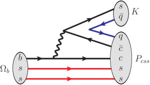
Figure 2: The production process involved in the predicted hidden-charm pentaquarks with double strangeness.

Appendix A Relevant subpotentials

The effective potentials for these discussed processes are expressed as

$$\mathcal{V}^{\Xi_{c}\bar{D}_{s}\rightarrow\Xi_{c}\bar{D}_{s}} = 2AY_{\sigma}+\frac{E}{2}Y_{\phi},$$ (1.1)

$$\mathcal{V}^{\Xi_{c}\bar{D}_{s}\rightarrow\Xi_{c}^{\prime}\bar{D}_{s}^{*}} = -\frac{C}{3\sqrt{6}}\left[\mathcal{A}_{1}\mathcal{O}_{r}+\mathcal{A}_{2}\mathcal{P}_{r}\right]Y_{\eta 1}$$ (1.2)

$$+\frac{2F}{3\sqrt{6}}\left[2\mathcal{A}_{1}\mathcal{O}_{r}-\mathcal{A}_{2}\mathcal{P}_{r}\right]Y_{\phi 1},$$

$$\mathcal{V}^{\Xi_{c}\bar{D}_{s}\rightarrow\Xi_{c}^{*}\bar{D}_{s}^{*}} = \frac{C}{3\sqrt{2}}\left[\mathcal{A}_{3}\mathcal{O}_{r}+\mathcal{A}_{4}\mathcal{P}_{r}\right]Y_{\eta 2}$$ (1.3)

$$-\frac{\sqrt{2}F}{3}\left[2\mathcal{A}_{3}\mathcal{O}_{r}-\mathcal{A}_{4}\mathcal{P}_{r}\right]Y_{\phi 2},$$

$$\mathcal{V}^{\Xi_{c}^{\prime}\bar{D}_{s}\rightarrow\Xi_{c}^{\prime}\bar{D}_{s}} = -BY_{\sigma}-\frac{G}{4}Y_{\phi},$$ (1.4)

$$\mathcal{V}^{\Xi_{c}^{\prime}\bar{D}_{s}\rightarrow\Xi_{c}\bar{D}_{s}^{*}} = -\frac{C}{3\sqrt{6}}\left[\mathcal{A}_{1}\mathcal{O}_{r}+\mathcal{A}_{2}\mathcal{P}_{r}\right]Y_{\eta 3}$$ (1.5)

$$+\frac{2F}{3\sqrt{6}}\left[2\mathcal{A}_{1}\mathcal{O}_{r}-\mathcal{A}_{2}\mathcal{P}_{r}\right]Y_{\phi 3},$$

$$\mathcal{V}^{\Xi_{c}^{\prime}\bar{D}_{s}\rightarrow\Xi_{c}^{*}\bar{D}_{s}} = \frac{B}{\sqrt{3}}\mathcal{A}_{5}Y_{\sigma 4}+\frac{G}{4\sqrt{3}}\mathcal{A}_{5}Y_{\phi 4},$$ (1.6)

$$\mathcal{V}^{\Xi_{c}^{\prime}\bar{D}_{s}\rightarrow\Xi_{c}^{\prime}\bar{D}_{s}^{*}} = \frac{D}{18}\left[\mathcal{A}_{1}\mathcal{O}_{r}+\mathcal{A}_{2}\mathcal{P}_{r}\right]Y_{\eta 5}$$ (1.7)

$$+\frac{H}{9}\left[2\mathcal{A}_{1}\mathcal{O}_{r}-\mathcal{A}_{2}\mathcal{P}_{r}\right]Y_{\phi 5},$$

$$\mathcal{V}^{\Xi_{c}^{\prime}\bar{D}_{s}\rightarrow\Xi_{c}^{*}\bar{D}_{s}^{*}} = -\frac{D}{12\sqrt{3}}\left[\mathcal{A}_{6}\mathcal{O}_{r}+\mathcal{A}_{7}\mathcal{P}_{r}\right]Y_{\eta 6}$$ (1.8)

$$-\frac{H}{6\sqrt{3}}\left[2\mathcal{A}_{6}\mathcal{O}_{r}-\mathcal{A}_{7}\mathcal{P}_{r}\right]Y_{\phi 6},$$

$$\mathcal{V}^{\Xi_{c}\bar{D}_{s}^{*}\rightarrow\Xi_{c}\bar{D}_{s}^{*}} = 2A\mathcal{A}_{8}Y_{\sigma}+\frac{E}{2}\mathcal{A}_{8}Y_{\phi},$$ (1.9)

$$\mathcal{V}^{\Xi_{c}\bar{D}_{s}^{*}\rightarrow\Xi_{c}^{*}\bar{D}_{s}} = \frac{C}{3\sqrt{2}}\left[\mathcal{A}_{9}\mathcal{O}_{r}+\mathcal{A}_{10}\mathcal{P}_{r}\right]Y_{\eta 7}$$ (1.10)

$$-\frac{\sqrt{2}F}{3}\left[2\mathcal{A}_{9}\mathcal{O}_{r}-\mathcal{A}_{10}\mathcal{P}_{r}\right]Y_{\phi 7},$$

$$\mathcal{V}^{\Xi_{c}\bar{D}_{s}^{*}\rightarrow\Xi_{c}^{\prime}\bar{D}_{s}^{*}} = -\frac{C}{3\sqrt{6}}\left[\mathcal{A}_{11}\mathcal{O}_{r}+\mathcal{A}_{12}\mathcal{P}_{r}\right]Y_{\eta 8}$$ (1.11)

$$+\frac{2F}{3\sqrt{6}}\left[2\mathcal{A}_{11}\mathcal{O}_{r}-\mathcal{A}_{12}\mathcal{P}_{r}\right]Y_{\phi 8},$$

$$\mathcal{V}^{\Xi_{c}\bar{D}_{s}^{*}\rightarrow\Xi_{c}^{*}\bar{D}_{s}^{*}} = \frac{C}{3\sqrt{2}}\left[\mathcal{A}_{13}\mathcal{O}_{r}+\mathcal{A}_{14}\mathcal{P}_{r}\right]Y_{\eta 9}$$ (1.12)

$$-\frac{\sqrt{2}F}{3}\left[2\mathcal{A}_{13}\mathcal{O}_{r}-\mathcal{A}_{14}\mathcal{P}_{r}\right]Y_{\phi 9},$$

$$\mathcal{V}^{\Xi_{c}^{*}\bar{D}_{s}\rightarrow\Xi_{c}^{*}\bar{D}_{s}} = -B\mathcal{A}_{15}Y_{\sigma}-\frac{G}{4}\mathcal{A}_{15}Y_{\phi},$$ (1.13)

$$\mathcal{V}^{\Xi_{c}^{*}\bar{D}_{s}\rightarrow\Xi_{c}^{\prime}\bar{D}_{s}^{*}} = \frac{D}{12\sqrt{3}}\left[\mathcal{A}_{16}\mathcal{O}_{r}+\mathcal{A}_{17}\mathcal{P}_{r}\right]Y_{\eta 10}$$ (1.14)

$$+\frac{H}{6\sqrt{3}}\left[2\mathcal{A}_{16}\mathcal{O}_{r}-\mathcal{A}_{17}\mathcal{P}_{r}\right]Y_{\phi 10},$$

$$\mathcal{V}^{\Xi_{c}^{*}\bar{D}_{s}\rightarrow\Xi_{c}^{*}\bar{D}_{s}^{*}} = \frac{D}{12}\left[\mathcal{A}_{18}\mathcal{O}_{r}+\mathcal{A}_{19}\mathcal{P}_{r}\right]Y_{\eta 11}$$ (1.15)

$$+\frac{H}{6}\left[2\mathcal{A}_{18}\mathcal{O}_{r}-\mathcal{A}_{19}\mathcal{P}_{r}\right]Y_{\phi 11},$$

$$\mathcal{V}^{\Xi_{c}^{\prime}\bar{D}_{s}^{*}\rightarrow\Xi_{c}^{\prime}\bar{D}_{s}^{*}} = -B\mathcal{A}_{8}Y_{\sigma}+\frac{D}{18}\left[\mathcal{A}_{11}\mathcal{O}_{r}+\mathcal{A}_{12}\mathcal{P}_{r}\right]Y_{\eta}$$ (1.16)

$$-\frac{G}{4}\mathcal{A}_{8}Y_{\phi}-\frac{H}{9}\left[2\mathcal{A}_{11}\mathcal{O}_{r}-\mathcal{A}_{12}\mathcal{P}_{r}\right]Y_{\phi},$$

$$\mathcal{V}^{\Xi_{c}^{\prime}\bar{D}_{s}^{*}\rightarrow\Xi_{c}^{*}\bar{D}_{s}^{*}} = \frac{B}{\sqrt{3}}\mathcal{A}_{20}Y_{\sigma 12}+\frac{D}{12\sqrt{3}}\left[\mathcal{A}_{21}\mathcal{O}_{r}+\mathcal{A}_{22}\mathcal{P}_{r}\right]Y_{\eta 12}$$

$$+\frac{G\mathcal{A}_{20}}{4\sqrt{3}}Y_{\phi 12}-\frac{H}{6\sqrt{3}}\left[2\mathcal{A}_{21}\mathcal{O}_{r}-\mathcal{A}_{22}\mathcal{P}_{r}\right]Y_{\phi 12},$$

$$\mathcal{V}^{\Xi_{c}^{*}\bar{D}_{s}^{*}\rightarrow\Xi_{c}^{*}\bar{D}_{s}^{*}} = -B\mathcal{A}_{23}Y_{\sigma}-\frac{D}{12}\left[\mathcal{A}_{24}\mathcal{O}_{r}+\mathcal{A}_{25}\mathcal{P}_{r}\right]Y_{\eta}$$ (1.18)

$$-\frac{G}{4}\mathcal{A}_{23}Y_{\phi}+\frac{H}{6}\left[2\mathcal{A}_{24}\mathcal{O}_{r}-\mathcal{A}_{25}\mathcal{P}_{r}\right]Y_{\phi}.$$

Here, $\mathcal{O}_{r}=\frac{1}{r^{2}}\frac{\partial}{\partial r}r^{2}\frac{\partial}{\partial r}$ and $\mathcal{P}_{r}=r\frac{\partial}{\partial r}\frac{1}{r}\frac{\partial}{\partial r}$. Additionally, we also define several variables, which include $A=l_{B}g_{S}$, $B=l_{S}g_{S}$, $C=g_{4}g/f_{\pi}^{2}$, $D=g_{1}g/f_{\pi}^{2}$, $E=\beta\beta_{B}g_{V}^{2}$, $F=\lambda\lambda_{I}g_{V}^{2}$, $G=\beta\beta_{S}g_{V}^{2}$, and $H=\lambda\lambda_{S}g_{V}^{2}$. The function $Y_{i}$ is defined as

$$Y_{i}\equiv\dfrac{e^{-m_{i}r}-e^{-\Lambda_{i}r}}{4\pi r}-\dfrac{\Lambda_{i}^{2}-m_{i}^{2}}{8\pi\Lambda_{i}}e^{-\Lambda_{i}r}.$$ (1.19)

Here, $m_{i}=\sqrt{m^{2}-q_{i}^{2}}$ and $\Lambda_{i}=\sqrt{\Lambda^{2}-q_{i}^{2}}$ with $q_{i}^{2}=(m_{A}^{2}+m_{D}^{2}-m_{B}^{2}-m_{C}^{2})^{2}/(2m_{C}+2m_{D})^{2}$ for the processes $AB\to CD$.

In the above OBE effective potentials, we also introduce several operators $\mathcal{A}_{k}$, i.e.,

$$\mathcal{A}_{1} = \chi^{\dagger}_{3}\left({\bm{\sigma}}\cdot{\bm{\epsilon}^{\dagger}_{4}}\right)\chi_{1},$$

$$\mathcal{A}_{2} = \chi^{\dagger}_{3}T({\bm{\sigma}},{\bm{\epsilon}^{\dagger}_{4}})\chi_{1},$$

$$\mathcal{A}_{3} = \sum_{a,b}C^{\frac{3}{2},a+b}_{\frac{1}{2}a,1b}\chi^{\dagger a}_{3}\left({\bm{\epsilon}^{\dagger b}_{3}}\cdot{\bm{\epsilon}^{\dagger}_{4}}\right)\chi_{1},$$

$$\mathcal{A}_{4} = \sum_{a,b}C^{\frac{3}{2},a+b}_{\frac{1}{2}a,1b}\chi^{\dagger a}_{3}T({\bm{\epsilon}^{\dagger b}_{3}},{\bm{\epsilon}^{\dagger}_{4}})\chi_{1},$$

$$\mathcal{A}_{5} = \sum_{a,b}C^{\frac{3}{2},a+b}_{\frac{1}{2}a,1b}\chi^{\dagger a}_{3}\left({\bm{\epsilon}^{\dagger b}_{3}}\cdot{\bm{\sigma}}\right)\chi_{1},$$

$$\mathcal{A}_{6} = \sum_{a,b}C^{\frac{3}{2},a+b}_{\frac{1}{2}a,1b}\chi^{\dagger a}_{3}\left[{\bm{\epsilon}^{\dagger}_{4}}\cdot\left(i{\bm{\sigma}}\times{\bm{\epsilon}^{\dagger b}_{3}}\right)\right]\chi_{1},$$

$$\mathcal{A}_{7} = \sum_{a,b}C^{\frac{3}{2},a+b}_{\frac{1}{2}a,1b}\chi^{\dagger a}_{3}T({\bm{\epsilon}^{\dagger}_{4}},i{\bm{\sigma}}\times{\bm{\epsilon}^{\dagger b}_{3}})\chi_{1},$$

$$\mathcal{A}_{8} = \chi^{\dagger}_{3}\left({\bm{\epsilon}^{\dagger}_{4}}\cdot{\bm{\epsilon}_{2}}\right)\chi_{1},$$

$$\mathcal{A}_{9} = \sum_{a,b}C^{\frac{3}{2},a+b}_{\frac{1}{2}a,1b}\chi^{\dagger a}_{3}\left({\bm{\epsilon}^{\dagger b}_{3}}\cdot{\bm{\epsilon}_{2}}\right)\chi_{1},$$

$$\mathcal{A}_{10} = \sum_{a,b}C^{\frac{3}{2},a+b}_{\frac{1}{2}a,1b}\chi^{\dagger a}_{3}T({\bm{\epsilon}^{\dagger b}_{3}},{\bm{\epsilon}_{2}})\chi_{1},$$

$$\mathcal{A}_{11} = \chi^{\dagger}_{3}\left[{\bm{\sigma}}\cdot\left(i{\bm{\epsilon}_{2}}\times{\bm{\epsilon}^{\dagger}_{4}}\right)\right]\chi_{1},$$

$$\mathcal{A}_{12} = \chi^{\dagger}_{3}T({\bm{\sigma}},i{\bm{\epsilon}_{2}}\times{\bm{\epsilon}^{\dagger}_{4}})\chi_{1},$$

$$\mathcal{A}_{13} = \sum_{a,b}C^{\frac{3}{2},a+b}_{\frac{1}{2}a,1b}\chi^{\dagger a}_{3}\left[{\bm{\epsilon}^{\dagger b}_{3}}\cdot\left(i{\bm{\epsilon}_{2}}\times{\bm{\epsilon}^{\dagger}_{4}}\right)\right]\chi_{1},$$

$$\mathcal{A}_{14} = \sum_{a,b}C^{\frac{3}{2},a+b}_{\frac{1}{2}a,1b}\chi^{\dagger a}_{3}T({\bm{\epsilon}^{\dagger b}_{3}},i{\bm{\epsilon}_{2}}\times{\bm{\epsilon}^{\dagger}_{4}})\chi_{1},$$

$$\mathcal{A}_{15} = \sum_{a,b,m,n}C^{\frac{3}{2},a+b}_{\frac{1}{2}a,1b}C^{\frac{3}{2},m+n}_{\frac{1}{2}m,1n}\chi^{\dagger a}_{3}\left({\bm{\epsilon}^{\dagger b}_{3}}\cdot{\bm{\epsilon}^{n}_{1}}\right)\chi^{m}_{1},$$

$$\mathcal{A}_{16} = \sum_{a,b}C^{\frac{3}{2},a+b}_{\frac{1}{2}a,1b}\chi^{\dagger}_{3}\left[{\bm{\epsilon}^{\dagger}_{4}}\cdot\left(i{\bm{\sigma}}\times{\bm{\epsilon}^{b}_{1}}\right)\right]\chi^{a}_{1},$$

$$\mathcal{A}_{17} = \sum_{a,b}C^{\frac{3}{2},a+b}_{\frac{1}{2}a,1b}\chi^{\dagger}_{3}T({\bm{\epsilon}^{\dagger}_{4}},i{\bm{\sigma}}\times{\bm{\epsilon}^{b}_{1}})\chi^{a}_{1},$$

$$\mathcal{A}_{18} = \sum_{a,b,m,n}C^{\frac{3}{2},a+b}_{\frac{1}{2}a,1b}C^{\frac{3}{2},m+n}_{\frac{1}{2}m,1n}\chi^{\dagger a}_{3}\left[{\bm{\epsilon}^{\dagger}_{4}}\cdot\left(i{\bm{\epsilon}^{n}_{1}}\times{\bm{\epsilon}^{\dagger b}_{3}}\right)\right]\chi^{m}_{1},$$

$$\mathcal{A}_{19} = \sum_{a,b,m,n}C^{\frac{3}{2},a+b}_{\frac{1}{2}a,1b}C^{\frac{3}{2},m+n}_{\frac{1}{2}m,1n}\chi^{\dagger a}_{3}T({\bm{\epsilon}^{\dagger}_{4}},i{\bm{\epsilon}^{n}_{1}}\times{\bm{\epsilon}^{\dagger b}_{3}})\chi^{m}_{1},$$

$$\mathcal{A}_{20} = \sum_{a,b}C^{\frac{3}{2},a+b}_{\frac{1}{2}a,1b}\chi^{\dagger a}_{3}\left({\bm{\sigma}}\cdot{\bm{\epsilon}^{\dagger b}_{3}}\right)\left({\bm{\epsilon}_{2}}\cdot{\bm{\epsilon}^{\dagger}_{4}}\right)\chi_{1},$$

$$\mathcal{A}_{21} = \sum_{a,b}C^{\frac{3}{2},a+b}_{\frac{1}{2}a,1b}\chi^{\dagger a}_{3}\left({\bm{\sigma}}\times{\bm{\epsilon}^{\dagger b}_{3}}\right)\cdot\left({\bm{\epsilon}_{2}}\times{\bm{\epsilon}^{\dagger}_{4}}\right)\chi_{1},$$

$$\mathcal{A}_{22} = \sum_{a,b}C^{\frac{3}{2},a+b}_{\frac{1}{2}a,1b}\chi^{\dagger a}_{3}T({\bm{\sigma}}\times{\bm{\epsilon}^{\dagger b}_{3}},{\bm{\epsilon}_{2}}\times{\bm{\epsilon}^{\dagger}_{4}})\chi_{1},$$

$$\mathcal{A}_{23} = \sum_{a,b,m,n}C^{\frac{3}{2},a+b}_{\frac{1}{2}a,1b}C^{\frac{3}{2},m+n}_{\frac{1}{2}m,1n}\chi^{\dagger a}_{3}\left({\bm{\epsilon}^{n}_{1}}\cdot{\bm{\epsilon}^{\dagger b}_{3}}\right)\left({\bm{\epsilon}_{2}}\cdot{\bm{\epsilon}^{\dagger}_{4}}\right)\chi^{m}_{1},$$

$$\mathcal{A}_{24} = \sum_{a,b,m,n}C^{\frac{3}{2},a+b}_{\frac{1}{2}a,1b}C^{\frac{3}{2},m+n}_{\frac{1}{2}m,1n}\chi^{\dagger a}_{3}\left({\bm{\epsilon}^{n}_{1}}\times{\bm{\epsilon}^{\dagger b}_{3}}\right)\cdot\left({\bm{\epsilon}_{2}}\times{\bm{\epsilon}^{\dagger}_{4}}\right)\chi^{m}_{1},$$

$$\mathcal{A}_{25} = \sum_{a,b,m,n}C^{\frac{3}{2},a+b}_{\frac{1}{2}a,1b}C^{\frac{3}{2},m+n}_{\frac{1}{2}m,1n}\chi^{\dagger a}_{3}T({\bm{\epsilon}^{n}_{1}}\times{\bm{\epsilon}^{\dagger b}_{3}},{\bm{\epsilon}_{2}}\times{\bm{\epsilon}^{\dagger}_{4}})\chi^{m}_{1}.$$

Here, the tensor force operator $T({\bm{x}},{\bm{y}})$ is expressed as $T({\bm{x}},{\bm{y}})=3\left(\hat{\bm{r}}\cdot{\bm{x}}\right)\left(\hat{\bm{r}}\cdot{\bm{y}}\right)-{\bm{x}}\cdot{\bm{y}}$ with $\hat{\bm{r}}={\bm{r}}/|{\bm{r}}|$. In Table 6, we present the obtained relevant matrix elements $\langle f|\mathcal{A}_{k}|i\rangle$, which will be used in our calculation.

Table 6: Matrix elements $\langle f|\mathcal{A}_{k}|i\rangle$ for the operators $\mathcal{A}_{k}$, which are obtained by sandwiching these operators between the relevant spin-orbit wave functions.

$S$-$D$ wave mixing effect				Coupled channel effect
Spin	$J=1/2$	$J=3/2$	$J=5/2$	$J=1/2$	$J=3/2$
$\langle\mathcal{A}_{8}\rangle$	diag(1,1)	diag(1,1,1)	$/$	$\mathcal{A}_{1}=\sqrt{3}$	$\mathcal{A}_{9}=1$
$\langle\mathcal{A}_{11}\rangle$	diag($-2$,$1$)	diag($1$,$-2$,$1$)	$/$	$\mathcal{A}_{3}=-\sqrt{2}$	$\mathcal{A}_{13}=-\sqrt{\frac{5}{3}}$
$\langle\mathcal{A}_{12}\rangle$	$\left(\begin{array}[]{cc}0&-\sqrt{2}\\ -\sqrt{2}&-2\end{array}\right)$	$\left(\begin{array}[]{ccc}0&1&2\\ 1&0&-1\\ 2&-1&0\end{array}\right)$	$/$	$\begin{array}[]{l}\mathcal{A}_{6}=\sqrt{2}\\ \mathcal{A}_{13}=-\sqrt{\frac{2}{3}}\\ \mathcal{A}_{21}=-\sqrt{\frac{2}{3}}\end{array}$	$\begin{array}[]{l}\mathcal{A}_{16}=1\\ \mathcal{A}_{18}=\sqrt{\frac{5}{3}}\\ \mathcal{A}_{21}=-\sqrt{\frac{5}{3}}\end{array}$
$\langle\mathcal{A}_{15}\rangle$	$/$	diag(1,1)	$/$
$\langle\mathcal{A}_{23}\rangle$	diag(1,1,1)	diag(1,1,1,1)	diag(1,1,1,1)
$\langle\mathcal{A}_{24}\rangle$	diag($\frac{5}{3}$,$\frac{2}{3}$,$-1$)	diag($\frac{2}{3}$,$\frac{5}{3}$,$\frac{2}{3}$,$-1$)	diag($-1$,$\frac{5}{3}$,$\frac{2}{3}$,$-1$)
$\langle\mathcal{A}_{25}\rangle$	$\left(\begin{array}[]{ccc}0&-\frac{7}{3\sqrt{5}}&\frac{2}{\sqrt{5}}\\ -\frac{7}{3\sqrt{5}}&\frac{16}{15}&-\frac{1}{5}\\ \frac{2}{\sqrt{5}}&-\frac{1}{5}&\frac{8}{5}\end{array}\right)$	$\left(\begin{array}[]{cccc}0&\frac{7}{3\sqrt{10}}&-\frac{16}{15}&-\frac{\sqrt{7}}{5\sqrt{2}}\\ \frac{7}{3\sqrt{10}}&0&-\frac{7}{3\sqrt{10}}&-\frac{2}{\sqrt{35}}\\ -\frac{16}{15}&-\frac{7}{3\sqrt{10}}&0&-\frac{1}{\sqrt{14}}\\ -\frac{\sqrt{7}}{5\sqrt{2}}&-\frac{2}{\sqrt{35}}&-\frac{1}{\sqrt{14}}&\frac{4}{7}\end{array}\right)$	$\left(\begin{array}[]{cccc}0&\frac{2}{\sqrt{15}}&\frac{\sqrt{7}}{5\sqrt{3}}&-\frac{2\sqrt{14}}{5}\\ \frac{2}{\sqrt{15}}&0&\frac{\sqrt{7}}{3\sqrt{5}}&-\frac{4\sqrt{2}}{\sqrt{105}}\\ \frac{\sqrt{7}}{5\sqrt{3}}&\frac{\sqrt{7}}{3\sqrt{5}}&-\frac{16}{21}&-\frac{\sqrt{2}}{7\sqrt{3}}\\ -\frac{2\sqrt{14}}{5}&-\frac{4\sqrt{2}}{\sqrt{105}}&-\frac{\sqrt{2}}{7\sqrt{3}}&-\frac{4}{7}\end{array}\right)$

References

• (1) Talk given by M. Z. Wang, On behalf of the LHCb Collaboration at Implications workshop 2020, see https://indico.cern.ch/event/857473/timetable/#32-exotic-hadrons-experimental.
• (2) R. Chen, J. He and X. Liu, Possible strange hidden-charm pentaquarks from $\Sigma_{c}^{(*)}\bar{D}_{s}^{*}$ and $\Xi^{(^{\prime},*)}_{c}\bar{D}^{*}$ interactions, Chin. Phys. C 41, no. 10, 103105 (2017).
• (3) J. J. Wu, R. Molina, E. Oset and B. S. Zou, Dynamically generated $N^{*}$ and $\Lambda^{*}$ resonances in the hidden charm sector around 4.3 GeV, Phys. Rev. C 84, 015202 (2011).
• (4) J. Hofmann and M. F. M. Lutz, Coupled-channel study of crypto-exotic baryons with charm, Nucl. Phys. A 763, 90 (2005).
• (5) V. V. Anisovich, M. A. Matveev, J. Nyiri, A. V. Sarantsev and A. N. Semenova, Nonstrange and strange pentaquarks with hidden charm, Int. J. Mod. Phys. A 30, no. 32, 1550190 (2015).
• (6) Z. G. Wang, Analysis of the ${\frac{1}{2}}^{\pm}$ pentaquark states in the diquark-diquark-antiquark model with QCD sum rules, Eur. Phys. J. C 76, no. 3, 142 (2016).
• (7) A. Feijoo, V. K. Magas, A. Ramos and E. Oset, A hidden-charm $S=-1$ pentaquark from the decay of $\Lambda_{b}$ into $J/\psi\eta\Lambda$ states, Eur. Phys. J. C 76, no. 8, 446 (2016).
• (8) J. X. Lu, E. Wang, J. J. Xie, L. S. Geng and E. Oset, The $\Lambda_{b}\rightarrow J/\psi K^{0}\Lambda$ reaction and a hidden-charm pentaquark state with strangeness, Phys. Rev. D 93, 094009 (2016).
• (9) C. W. Xiao, J. Nieves and E. Oset, Prediction of hidden charm strange molecular baryon states with heavy quark spin symmetry, Phys. Lett. B 799, 135051 (2019).
• (10) C. W. Shen, H. J. Jing, F. K. Guo and J. J. Wu, Exploring possible triangle singularities in the $\Xi^{-}_{b}\to K^{-}J/\psi\Lambda$ decay, Symmetry 12, no. 10, 1611 (2020).
• (11) H. X. Chen, L. S. Geng, W. H. Liang, E. Oset, E. Wang and J. J. Xie, Looking for a hidden-charm pentaquark state with strangeness S=-1 from $\Xi^{-}_{b}$ decay into $J/\psi K^{-}\Lambda$, Phys. Rev. C 93, no. 6, 065203 (2016).
• (12) B. Wang, L. Meng and S. L. Zhu, Spectrum of the strange hidden charm molecular pentaquarks in chiral effective field theory, Phys. Rev. D 101, no. 3, 034018 (2020).
• (13) Q. Zhang, B. R. He and J. L. Ping, Pentaquarks with the $qqs\bar{Q}Q$ configuration in the Chiral Quark Model, arXiv:2006.01042.
• (14) H. X. Chen, W. Chen, X. Liu and X. H. Liu, Establishing the first hidden-charm pentaquark with strangeness, arXiv:2011.01079.
• (15) F. Z. Peng, M. J. Yan, M. Sánchez Sánchez and M. P. Valderrama, The $P_{cs}(4459)$ pentaquark from a combined effective field theory and phenomenological perspectives, arXiv:2011.01915.
• (16) R. Chen, Can the newly $P_{cs}(4459)$ be a strange hidden-charm $\Xi_{c}\bar{D}^{*}$ molecular pentaquarks?, arXiv:2011.07214.
• (17) H. X. Chen, Hidden-charm pentaquark states through the current algebra: From their productions to decays, arXiv:2011.07187.
• (18) M. Z. Liu, Y. W. Pan and L. S. Geng, Can discovery of hidden charm strange pentaquark states help determine the spins of $P_{c}(4440)$ and $P_{c}(4457)$?, arXiv:2011.07935.
• (19) R. Aaij et al. [LHCb Collaboration], Observation of $J/\psi$ Resonances Consistent with Pentaquark States in $\Lambda_{b}^{0}\rightarrow J/\psi K^{-}p$ Decays, Phys. Rev. Lett.  115, 072001 (2015).
• (20) R. Aaij et al. (LHCb Collaboration), Observation of a Narrow Pentaquark State, $P_{c}(4312)^{+}$, and of Two-Peak Structure of the $P_{c}(4450)^{+}$, Phys. Rev. Lett.  122, 222001 (2019).
• (21) X. Q. Li and X. Liu, A possible global group structure for exotic states, Eur. Phys. J. C 74, 3198 (2014).
• (22) J. J. Wu, R. Molina, E. Oset and B. S. Zou, Prediction of narrow $N^{*}$ and $\Lambda^{*}$ resonances with hidden charm above 4 GeV, Phys. Rev. Lett.  105, 232001 (2010).
• (23) M. Karliner and J. L. Rosner, New Exotic Meson and Baryon Resonances from Doubly-Heavy Hadronic Molecules, Phys. Rev. Lett.  115, 122001 (2015).
• (24) W. L. Wang, F. Huang, Z. Y. Zhang, and B. S. Zou, $\Sigma_{c}\bar{D}$ and $\Lambda_{c}\bar{D}$ states in a chiral quark model, Phys. Rev. C 84, 015203 (2011).
• (25) Z. C. Yang, Z. F. Sun, J. He, X. Liu, and S. L. Zhu, The possible hidden-charm molecular baryons composed of anti-charmed meson and charmed baryon, Chin. Phys. C 36, 6 (2012).
• (26) J. J. Wu, T.-S. H. Lee, and B. S. Zou, Nucleon resonances with hidden charm in coupled-channel Models, Phys. Rev. C 85, 044002 (2012).
• (27) R. Chen, X. Liu, X. Q. Li, and S. L. Zhu, Identifying Exotic Hidden-Charm Pentaquarks, Phys. Rev. Lett.  115, 132002 (2015).
• (28) H. X. Chen, W. Chen, X. Liu, and S. L. Zhu, The hidden-charm pentaquark and tetraquark states, Phys. Rep.  639, 1 (2016).
• (29) Y. R. Liu, H. X. Chen, W. Chen, X. Liu, and S. L. Zhu, Pentaquark and tetraquark states, Prog. Part. Nucl. Phys.  107, 237 (2019).
• (30) S. L. Olsen, T. Skwarnicki, and D. Zieminska, Nonstandard heavy mesons and baryons: Experimental evidence, Rev. Mod. Phys.  90, 015003 (2018).
• (31) F. K. Guo, C. Hanhart, U. G. Mei$\ss$ner, Q. Wang, Q. Zhao, and B. S. Zou, Hadronic molecules, Rev. Mod. Phys.  90, 015004 (2018).
• (32) R. Aaij et al. [LHCb], Physics case for an LHCb Upgrade II-Opportunities in flavour physics, and beyond, in the HL-LHC era, arXiv:1808.08865.
• (33) F. L. Wang and X. Liu, Exotic double-charm molecular states with hidden or open strangeness and around $4.5\sim 4.7$ GeV, Phys. Rev. D 102, 094006 (2020).
• (34) F. L. Wang, R. Chen, Z. W. Liu, and X. Liu, Probing new types of $P_{c}$ states inspired by the interaction between $S$-wave charmed baryon and anti-charmed meson in a $\bar{T}$ doublet, Phys. Rev. C 101, 025201 (2020).
• (35) M. B. Wise, Chiral perturbation theory for hadrons containing a heavy quark, Phys. Rev. D 45, R2188 (1992).
• (36) R. Casalbuoni, A. Deandrea, N. Di Bartolomeo, R. Gatto, F. Feruglio, and G. Nardulli, Light vector resonances in the effective chiral Lagrangian for heavy mesons, Phys. Lett. B 292, 371 (1992).
• (37) R. Casalbuoni, A. Deandrea, N. Di Bartolomeo, R. Gatto, F. Feruglio, and G. Nardulli, Phenomenology of heavy meson chiral Lagrangians, Phys. Rep.  281, 145 (1997).
• (38) T. M. Yan, H. Y. Cheng, C. Y. Cheung, G. L. Lin, Y. C. Lin, and H. L. Yu, Heavy quark symmetry and chiral dynamics, Phys. Rev. D 46, 1148 (1992); [Phys. Rev. D 55, 5851E (1997)].
• (39) M. Bando, T. Kugo and K. Yamawaki, Nonlinear Realization and Hidden Local Symmetries, Phys. Rept.  164, 217 (1988).
• (40) M. Harada and K. Yamawaki, Hidden local symmetry at loop: A New perspective of composite gauge boson and chiral phase transition, Phys. Rept.  381, 1 (2003).
• (41) G. J. Ding, Are $Y(4260)$ and $Z_{2}^{+}$(4250) ${\rm D_{1}D}$ or ${\rm D_{0}D^{*}}$ hadronic molecules? Phys. Rev. D 79, 014001 (2009).
• (42) R. Chen, A. Hosaka, and X. Liu, Searching for possible $\Omega_{c}$-like molecular states from meson-baryon interaction, Phys. Rev. D 97, 036016 (2018).
• (43) R. Chen, F. L. Wang, A. Hosaka and X. Liu, Exotic triple-charm deuteronlike hexaquarks, Phys. Rev. D 97, no.11, 114011 (2018).
• (44) G. Breit, The effect of retardation on the interaction of two electrons, Phys. Rev.  34, 553 (1929).
• (45) G. Breit, The fine structure of HE as a test of the spin interactions of two electrons, Phys. Rev.  36, 383 (1930).
• (46) N. A. Tornqvist, From the deuteron to deusons, an analysis of deuteron-like meson-meson bound states, Z. Phys. C 61, 525 (1994).
• (47) N. A. Tornqvist, On deusons or deuteron-like meson-meson bound states, Nuovo Cim. Soc. Ital. Fis. 107A, 2471 (1994).
• (48) F. L. Wang, R. Chen, Z. W. Liu, and X. Liu, Possible triple-charm molecular pentaquarks from $\Xi_{cc}D_{1}/\Xi_{cc}D_{2}^{*}$ interactions, Phys. Rev. D 99, 054021 (2019).
• (49) R. Chen, A. Hosaka and X. Liu, Prediction of triple-charm molecular pentaquarks, Phys. Rev. D 96, no. 11, 114030 (2017).
• (50) D. O. Riska and G. E. Brown, Nucleon resonance transition couplings to vector mesons, Nucl. Phys. A 679, 577 (2001).
• (51) R. Chen, Z. F. Sun, X. Liu and S. L. Zhu, Strong LHCb evidence supporting the existence of the hidden-charm molecular pentaquarks, Phys. Rev. D 100, no. 1, 011502 (2019).
• (52) P. A. Zyla et al. [Particle Data Group], Review of Particle Physics, PTEP 2020, no.8, 083C01 (2020).