Bayesian Bootstrap Spike-and-Slab LASSO

Abstract

The impracticality of posterior sampling has prevented the widespread adoption of spike-and-slab priors in high-dimensional applications. To alleviate the computational burden, optimization strategies have been proposed that quickly find local posterior modes. Trading off uncertainty quantification for computational speed, these strategies have enabled spike-and-slab deployments at scales that would be previously unfeasible. We build on one recent development in this strand of work: the Spike-and-Slab LASSO procedure of Ročková and George (2018). Instead of optimization, however, we explore multiple avenues for posterior sampling, some traditional and some new. Intrigued by the speed of Spike-and-Slab LASSO mode detection, we explore the possibility of sampling from an approximate posterior by performing MAP optimization on many independently perturbed datasets. To this end, we explore Bayesian bootstrap ideas and introduce a new class of jittered Spike-and-Slab LASSO priors with random shrinkage targets. These priors are a key constituent of the Bayesian Bootstrap Spike-and-Slab LASSO (BB-SSL) method proposed here. BB-SSL turns fast optimization into approximate posterior sampling. Beyond its scalability, we show that BB-SSL has a strong theoretical support. Indeed, we find that the induced pseudo-posteriors contract around the truth at a near-optimal rate in sparse normal-means and in high-dimensional regression. We compare our algorithm to the traditional Stochastic Search Variable Selection (under Laplace priors) as well as many state-of-the-art methods for shrinkage priors. We show, both in simulations and on real data, that our method fares very well in these comparisons, often providing substantial computational gains.

Keywords: Bayesian Bootstrap, Posterior Contraction, Spike-and-Slab LASSO, Weighted Likelihood Bootstrap.

1 Posterior Sampling under Shrinkage Priors

Variable selection is arguably one of the most widely used dimension reduction techniques in modern statistics. The default Bayesian approach to variable selection assigns a probabilistic blanket over models via spike-and-slab priors Mitchell and Beauchamp (1988); George and McCulloch (1993). The major conceptual appeal of the spike-and-slab approach is the availability of uncertainty quantification for both model parameters as well as models themselves (Madigan and Raftery (1994)). However, practical costs of posterior sampling can be formidable given the immense scope of modern analyses. The main thrust of this work is to extend the reach of existing posterior sampling algorithms in new faster directions.

This paper focuses on the canonical linear regression model, where a vector of responses $\boldsymbol{Y}=(Y_{1},\dots,Y_{n})^{T}$ is stochastically linked to fixed predictors $\boldsymbol{x}_{i}\in\mathbb{R}^{p}$ through

$$Y_{i}=\boldsymbol{x}_{i}^{T}\boldsymbol{\beta}_{0}+\epsilon_{i}\quad\text{with}\quad\epsilon_{i}\overset{\text{i.i.d}}{\sim}\mathcal{N}(0,\sigma^{2})\quad\text{for}\quad 1\leq i\leq n,$$ (1)

where $\sigma^{2}>0$ and where $\boldsymbol{\beta}_{0}\in\mathbb{R}^{p}$ is a possibly sparse vector of regression coefficients. In this work, we assume that $\sigma^{2}$ is known and we refer to Moran et al. (2019) for elaborations with an unknown variance. We assume that the vector $\boldsymbol{Y}$ and the regressors $\boldsymbol{X}=[\boldsymbol{X}_{1},\dots,\boldsymbol{X}_{p}]$ have been centered and, thereby, we omit the intercept. In the presence of uncertainty about which subset of $\boldsymbol{\beta}_{0}$ is in fact nonzero, one can assign a prior distribution over the regression coefficients $\boldsymbol{\beta}=(\beta_{1},\dots,\beta_{p})^{T}$ as well as the pattern of nonzeroes $\boldsymbol{\gamma}=(\gamma_{1},\dots,\gamma_{p})^{T}$ where $\gamma_{j}\in\{0,1\}$ for whether or not the effect $\beta_{j}$ is active. This formalism can be condensed into the usual spike-and-slab prior form

$$\pi(\boldsymbol{\beta}\,|\>\boldsymbol{\gamma})=\prod_{j=1}^{p}[\gamma_{j}\psi_{1}(\beta_{j})+(1-\gamma_{j})\psi_{0}(\beta_{j})],\quad\mathbb{P}(\gamma_{j}=1\,|\>\theta)=\theta,\quad\theta\sim\mathrm{Beta}(a,b),$$ (2)

where $a,b>0$ are scale parameters and where $\psi_{0}(\cdot)$ is a highly concentrated prior density around zero (the spike) and $\psi_{1}(\cdot)$ is a diffuse density (the slab). The dual purpose of the spike-and-slab prior is to (a) shrink small signals towards zero and (b) keep large signals intact. The most popular incarnations of the spike-and-slab prior include: the point-mass spike (Mitchell and Beauchamp (1988)), the non-local slab priors (Johnson and Rossell (2012)), the Gaussian mixture (George and McCulloch (1993)), the Student mixture (Ishwaran and Rao (2005)). More recently, Ročková (2018a) proposed the Spike-and-Slab LASSO (SSL) prior, a mixture of two Laplace distributions $\psi_{0}(\beta)=\frac{\lambda_{0}}{2}\mathrm{e}^{-|\beta|\lambda_{0}}$ and $\psi_{1}(\beta)=\frac{\lambda_{1}}{2}\mathrm{e}^{-|\beta|\lambda_{1}}$ where $\lambda_{0}\gg\lambda_{1}$, which forms a continuum between the point-mass mixture prior and the LASSO prior (Park and Casella (2008)).

Posterior sampling under spike-and-slab priors is notoriously difficult. Dating back to at least 1993 (George and McCulloch, 1993), multiple advances have been made to speed up spike-and-slab posterior simulation (George and McCulloch (1997), Bottolo and Richardson (2010), Clyde et al. (2011), Hans (2009), Johndrow et al. (2020), Welling and Teh (2011), Xu et al. (2014)). More recently, several clever computational tricks have been suggested that avoid costly matrix inversions by using linear solvers (Bhattacharya et al., 2016) or by disregarding correlations between active and inactive coefficients (Narisetty et al., 2019). Neuronized priors have been proposed (Shin and Liu (2018)) that offer computational benefits by using close approximations to spike-and-slab priors without latent binary indicators. Modern applications have nevertheless challenged MCMC algorithms and new computational strategies are desperately needed to keep pace with big data.

Optimization strategies have shown great promise and enabled deployment of spike-and-slab priors at scales that would be previously unfeasible (Ročková and George (2014), Ročková and George (2018), Carbonetto and Stephens (2012)). Fast posterior mode detection is effective in structure discovery and data exploration, a little less so for inference. In this paper, we review and propose new strategies for posterior sampling under the Spike-and-Slab LASSO priors, filling the gap between exploratory data analysis and proper statistical inference.

We capitalize on the latest MAP optimization and MCMC developments to provide several posterior sampling implementations for the Spike-and-Slab LASSO method of Ročková and George (2018). The first one (presented in Algorithm 1) is exact and conventional, following in the footsteps of Stochastic Search Variable Selection (George and McCulloch, 1993)). The second one is approximate and new. The cornerstone of this strategy is the Weighted Likelihood Bootstrap (WLB) of Newton and Raftery (1994) which was recently resurrected in the context of posterior sampling with sparsity priors by Newton et al. (2020), Fong et al. (2019) and Ng and Newton (2020). The main idea behind WLB is to perform approximate sampling by independently optimizing randomly perturbed likelihood functions. We extend the WLB framework by incorporating perturbations both in the likelihood and in the prior. The main contributions of this work are two-fold. First, we introduce BB-SSL (Bayesian Bootstrap Spike-and-Slab LASSO), a novel algorithm for approximate posterior sampling in high-dimensional regression under Spike-and-Slab LASSO priors. Second, we show that suitable “perturbations” lead to approximate posteriors that contract around the truth at the same speed (rate) as the actual posterior. These theoretical results have nontrivial practical implications as they offer guidance on the choice of the distribution for perturbing weights. Up until now, theoretical properties of WLB have largely concentrated on consistency statements in low dimensions for iid data (Newton and Raftery (1994)). More recently, Ng and Newton (2020) established conditional consistency (asymptotic normality) in the context of LASSO regression for a fixed dimensionality and model selection consistency for a growing dimensionality. Our theoretical results also allow the dimensionality to increase with the sample size and go beyond mere consistency by showing that BB-SSL leads to rate-optimal estimation in sparse normal-means and high-dimensional regression under standard assumptions. Last but not least, we make thorough comparisons with the gold standard (i.e. exact MCMC sampling) on multiple simulated and real datasets, concluding that the proposed algorithm is scalable and reliable in practice. BB-SSL is (a) unapologetically parallelisable, and (b) it does not require costly matrix inversions (due to its coordinate-wise optimization nature), thereby having the potential to meet the demands of large datasets.

The structure of this paper is as follows. Section 1.1 introduces the notation. Section 2 revisits Spike-and-Slab LASSO and presents a traditional algorithm for posterior sampling. Section 3 investigates performance of weighted Bayesian bootstrap, the building block of this work, in high dimensions. In Section 4, we introduce BB-SSL and present our theoretical study showing rate-optimality as well as its connection with other bootstrap methods. Section 5 shows simulated examples and Section 6 shows performance on real data. We conclude the paper with a discussion in Section 7.

1.1 Notation

With $\phi(y;\mu;\sigma^{2})$ we denote the Gaussian density with a mean $\mu$ and a variance $\sigma^{2}$. We use $\xrightarrow{\text{d}}$ to denote convergence in distribution. We write $a_{n}=O_{p}(b_{n})$ if for any $\epsilon>0$, there exist finite $M>0$ and $N>0$ such that $\mathbb{P}(|a_{n}/b_{n}|>M)<\epsilon$ for any $n>N$. We write $a_{n}=o_{p}(b_{n})$ if for any $\epsilon>0$, $\lim_{n\rightarrow\infty}\mathbb{P}(|a_{n}/b_{n}|>\epsilon)=0$. We also write $a_{n}=O(b_{n})$ as $a_{n}\lesssim b_{n}$. We use $a\asymp b$ if $a\lesssim b$ and $b\lesssim a$. We use $a_{n}\gg b_{n}$ to denote $b_{n}=o(a_{n})$ and $a_{n}\ll b_{n}$ to denote $a_{n}=o(b_{n})$. We denote with $\boldsymbol{X}_{A}$ a sub-matrix consisting of columns of $\boldsymbol{X}$’s indexed by a subset $A\subset\left\{1,\cdots,p\right\}$ and with $\boldsymbol{P}_{A}$ the orthogonal projection to the range of $\boldsymbol{X}_{A}$ (Zhang and Zhang, 2012), i.e., $\boldsymbol{P}_{A}=\boldsymbol{X}_{A}\boldsymbol{X}_{A}^{+}$ where $\boldsymbol{X}_{A}^{+}$ is the Moore-Penrose inverse of $\boldsymbol{X}_{A}$. We denote with $\|\boldsymbol{X}\|$ the matrix operator norm of $\boldsymbol{X}$.

2 Spike-and-Slab LASSO Revisited

The Spike-and-Slab LASSO (SSL) procedure of Ročková and George (2018) recently emerged as one of the more successful non-convex penalized likelihood methods. Various SSL incarnations have spawned since its introduction, including a version for group shrinkage (Bai et al. (2020), Tang et al. (2018)), survival analysis (Tang et al. (2017)), varying coefficient models (Bai et al. (2020)) and/or Gaussian graphical models (Deshpande et al. (2019), Li et al. (2019)). The original procedure proposed for Gaussian regression targets a posterior mode

$$\smash{\widehat{\boldsymbol{\beta}}}=\arg\max_{\boldsymbol{\beta}\in\mathbb{R}^{p}}\left\{\prod_{i=1}^{n}\phi(Y_{i};\boldsymbol{x}_{i}^{T}\boldsymbol{\beta};\sigma^{2})\times\int_{\theta}\prod_{j=1}^{p}\pi(\beta_{j}\,|\>\theta)d\pi(\theta)\right\},$$ (3)

where $\pi(\beta_{j}\,|\>\theta)=\theta\psi_{1}(\beta_{j})+(1-\theta)\psi_{0}(\beta_{j})$ is obtained from (2) by integrating out the missing indicator $\gamma_{j}$ and by deploying $\psi_{1}(\beta_{j})=\lambda_{1}/2\mathrm{e}^{-|\beta_{j}|\lambda_{1}}$ and $\psi_{0}(\beta_{j})=\lambda_{0}/2\mathrm{e}^{-|\beta_{j}|\lambda_{0}}$ with $\lambda_{0}\gg\lambda_{1}$. Ročková and George (2018) develop a coordinate-ascent strategy which targets $\smash{\widehat{\boldsymbol{\beta}}}$ and which quickly finds (at least a local) mode of the posterior landscape. This strategy (summarized in Theorem 3.1 of Ročková and George (2018)) iteratively updates each $\smash{\widehat{\beta}}_{j}$ using an implicit equation

$$\smash{\widehat{\beta}}_{j}= \frac{1}{\|\boldsymbol{X}_{j}\|_{2}^{2}}\left(|z_{j}|-\sigma^{2}\lambda^{*}_{\smash{\widehat{\theta}}_{j}}(\smash{\widehat{\beta}}_{j})\right)_{+}\mathrm{sign}(z_{j})\times\mathbb{I}(|z_{j}|>\Delta_{j})$$ (4)

where $\smash{\widehat{\theta}}_{j}=\mathbb{E}[\theta\,|\>\smash{\widehat{\boldsymbol{\beta}}}_{\backslash j}]$, $z_{j}=\boldsymbol{X}_{j}^{T}(\boldsymbol{Y}-\boldsymbol{X}_{\backslash j}\smash{\widehat{\boldsymbol{\beta}}}_{\backslash j})$ and $\Delta_{j}=\inf_{t>0}\left(\|\boldsymbol{X}_{j}\|^{2}t/2-\sigma^{2}\rho(t\,|\>\smash{\widehat{\theta}}_{j})/t\right)$ with $\rho(t\,|\>\theta)=-\lambda_{1}|t|+\log[p^{\star}_{\theta}(0)/p^{\star}_{\theta}(t)],$ where

$$\centering p^{\star}_{\theta}(t)=\frac{\theta\psi_{1}(t)}{\theta\psi_{1}(t)+(1-\theta)\psi_{0}(t)}\quad\text{and}\quad\lambda^{*}_{\theta}(t)=\lambda_{1}p^{\star}_{\theta}(t)+\lambda_{0}(1-p^{\star}_{\theta}(t)).\@add@centering$$ (5)

Ročková and George (2018) also provide fast updating schemes for $\Delta_{j}$ and $\smash{\widehat{\theta}}_{j}$. In this work, we are interested in sampling from the posterior as opposed to mode hunting.

One immediate strategy for sampling from the Spike-and-Slab LASSO posterior is the Stochastic Search Variable Selection (SSVS) algorithm of George and McCulloch (1993). One can regard the Laplace distribution (with a penalty $\lambda>0$) as a scale mixture of Gaussians with an exponential mixing distribution (with a rate $\lambda^{2}/2$ as in Park and Casella (2008)) and rewrite the SSL prior using the following hierarchical form:

$$\boldsymbol{\beta}\,|\>\boldsymbol{\tau} \sim\mathcal{N}(\textbf{0},D_{\boldsymbol{\tau}})\quad\text{with}\quad D_{\boldsymbol{\tau}}=\mathrm{Diag}(1/\tau_{1}^{2},1/\tau_{2}^{2},\cdots,1/\tau_{p}^{2}),$$

$$\boldsymbol{\tau}^{-1}\,|\>\boldsymbol{\gamma} \sim\prod_{j=1}^{p}\frac{\lambda_{j}^{2}}{2}\mathrm{e}^{-\lambda_{j}^{2}/2\tau_{j}^{2}},\quad\text{where}\quad\lambda_{j}=\gamma_{j}\lambda_{1}+(1-\gamma_{j})\lambda_{0},$$

$$\gamma_{j}\,|\>\theta \sim\mathrm{Bernoulli}(\theta)\quad\text{with}\quad\theta\sim\mathrm{Beta}(a,b),$$

where $\boldsymbol{\tau}^{-1}=(1/\tau_{1}^{2},\dots,1/\tau_{p}^{2})^{T}$ is the vector of variances. The conditional conjugacy of the SSL prior enables direct Gibbs sampling for $\boldsymbol{\beta}$ (see Algorithm 1 below). However, as with any other Gibbs sampler for Bayesian shrinkage models (Bhattacharya et al., 2015), this algorithm involves costly matrix inversions and can be quite slow when both $n$ and $p$ are large. In order to improve the MCMC computational efficiency when $p>n$, Bhattacharya et al. (2016) proposed a clever trick. By recasting the sampling step as a solution to a linear system, one can circumvent a Cholesky factorization which would otherwise have a complexity $O(n^{2}p)$ per iteration. Building on this development, Johndrow et al. (2020) developed a blocked Metropolis-within-Gibbs algorithm to sample from horseshoe posteriors (Carvalho et al., 2010) and designed an approximate algorithm which thresholds small effects based on the sparse structure of the target. The exact method has a per-step complexity $O(n^{2}p)$ while the approximate one has only $O(np)$. In similar vein, the Skinny Gibbs MCMC method of Narisetty et al. (2019) also bypasses large matrix inversions by independently sampling from active and inactive $\beta_{i}$’s. While the method is only approximate, it has a rather favorable computational complexity $O(np)$. A referee suggested another Gibbs sampler implementation with a complexity $O(np)$ which can be obtained by updating $(\beta_{j},\gamma_{j})$ one at a time while conditioning on the remaining $(\beta_{j},\gamma_{j})$’s (Geweke, 1991). While this implementation is very fast for point-mass spikes, the Spike-and-Slab LASSO prior requires sampling from a half-normal distribution which can be inefficient in practice. One-site Gibbs samplers also generally lead to slower mixing due to increased autocorrelation. In simulations, we find the performance of this method to be comparable with SSVS using Bhattacharya et al. (2016)’s trick. The detailed description of this algorithm is included in the Appendix (Section C).

The impressive speed of the Spike-and-Slab LASSO mode detection makes one wonder whether performing many independent optimizations on randomly perturbed datasets will lead to posterior simulation that is more economical. Moreover, one may wonder whether the induced approximate posterior is sufficiently close to the actual posterior $\pi(\boldsymbol{\beta}\,|\>\boldsymbol{Y})$ and/or whether it can be used for meaningful estimation/uncertainty quantification. We attempt to address these intriguing questions in the next sections.

Set: $\lambda_{0}\gg\lambda_{1},$ $a,b>0$, $T$ (number of MCMC iterations), $B$ (number of samples to discard as burn-in).

Initialize: $\boldsymbol{\beta}^{0}$ (e.g. LASSO solution after 10-fold cross validation) and $\boldsymbol{\tau}^{0}$.

for $t=1,2,\cdots,T$ do

                                                   ahoj

       (a) Sample $\boldsymbol{\beta}^{t}$ $\sim\mathcal{N}\left(\mu_{\boldsymbol{\gamma}},\Sigma_{\boldsymbol{\gamma}}\right)$, where $\Sigma_{\boldsymbol{\gamma}}=(\boldsymbol{X}^{T}\boldsymbol{X}/\sigma^{2}+D_{\boldsymbol{\tau}^{t-1}}^{-1})^{-1}$ and $\mu_{\boldsymbol{\gamma}}=\Sigma_{\boldsymbol{\gamma}}\boldsymbol{X}^{T}{\boldsymbol{Y}}/\sigma^{2}$.

       (b) Sample $(\tau_{j}^{t})^{2}\sim\mathrm{Inv}$-$\mathrm{Gaus}(\mu^{\prime}_{j},(\lambda^{\prime}_{j})^{2})$ for $j=1,2,\dots,p$ , where

$$\mu^{\prime}_{j}=\frac{|\lambda^{\prime}_{j}|}{|\beta_{j}^{t}|}\quad\text{and}\quad(\lambda^{\prime}_{j})^{2}=\gamma_{j}^{t-1}\lambda_{1}^{2}+(1-\gamma_{j}^{t-1})\lambda_{0}^{2}$$

(c) Sample $\gamma_{j}^{t}\sim\mathrm{Bernoulli}\left(\frac{\pi_{1}}{\pi_{1}+\pi_{0}}\right)$, where

$$\pi_{1}=\theta^{t-1}\lambda_{1}^{2}\mathrm{e}^{-\lambda_{1}^{2}/2(\tau_{j}^{t})^{2}}/2\quad\text{and}\quad\pi_{0}=(1-\theta^{t-1})\lambda_{0}^{2}\mathrm{e}^{-\lambda_{0}^{2}/2(\tau_{j}^{t})^{2}}/2.$$

(d) Sample $\theta^{t}\sim\mathrm{Beta}(\sum_{j=1}^{p}\gamma_{j}^{t}+a,p-\sum_{j=1}^{p}\gamma_{j}^{t}+b)$.

      

end for

Return: $\boldsymbol{\beta}^{t},\boldsymbol{\gamma}^{t},\theta^{t}$ where $t=B+1,B+2,\cdots,T$.

Algorithm 1 : SSVS

3 Likelihood Reweighting and Bayesian Bootstrap

The jumping-off point of our methodology is the weighted likelihood bootstrap (WLB) method introduced by Newton and Raftery (1994). The premise of WLB is to draw approximate samples from the posterior by independently maximizing randomly reweighted likelihood functions. Such a sampling strategy is computationally beneficial when, for instance, maximization is easier than Gibbs sampling from conditionals.

In the context of linear regression (1), the WLB method of Newton and Raftery (1994) will produce a series of draws $\widetilde{\boldsymbol{\beta}}_{t}$ by first sampling random weights $\boldsymbol{w}_{t}=(w_{1}^{t},w_{2}^{t},\cdots,w_{n}^{t})^{T}$ from some weight distribution $\pi(\boldsymbol{w})$ and then maximizing a reweighted likelihood

$$\widetilde{\boldsymbol{\beta}}_{t}=\arg\,\max_{\boldsymbol{\beta}}\widetilde{L}^{\boldsymbol{w}_{t}}(\boldsymbol{\beta},\sigma^{2};\boldsymbol{X}^{(n)},\boldsymbol{Y}^{(n)})$$ (6)

where

$$\widetilde{L}^{\boldsymbol{w}_{t}}(\boldsymbol{\beta},\sigma^{2};\boldsymbol{X}^{(n)},\boldsymbol{Y}^{(n)})=\prod_{i=1}^{n}\phi(Y_{i};\boldsymbol{x}_{i}^{T}\boldsymbol{\beta};\sigma^{2})^{w_{i}^{t}}.$$

Newton and Raftery (1994) argue that for certain weight distributions $\pi(\boldsymbol{w})$, the conditional distribution of $\widetilde{\boldsymbol{\beta}}_{t}$’s given the data can provide a good approximation to the posterior distribution of $\boldsymbol{\beta}$. Moreover, WLB was shown to have nice theoretical guarantees when the number of parameters does not grow. Namely, under uniform Dirichlet weights (more below) and iid data samples, WLB is consistent (i.e. concentrating on any arbitrarily small neighborhood around an MLE estimator) and asymptotically first-order correct (normal with the same centering) for almost every realization of the data. The WLB method, however, is only approximate and it does not naturally accommodate a prior. Uniform Dirichlet weights provide a higher-order asymptotic equivalence when one chooses the squared Jeffrey’s prior. However, for more general prior distributions (such as shrinkage priors considered here), the correspondence between the prior $\pi(\boldsymbol{\beta})$ and $\pi(\boldsymbol{w})$ is unknown. Newton and Raftery (1994) suggest post-processing the posterior samples with importance sampling to leverage prior information. This pertains to Efron (2012), who proposes a posterior sampling method for exponential family models with importance sampling on parametric bootstrap distributions.

Alternatively, Newton et al. (2020) suggested blending the prior directly into WLB by including a weighted prior term, i.e. replacing (6) with

$$\widetilde{\boldsymbol{\beta}}_{t}=\arg\,\max_{\boldsymbol{\beta}}\widetilde{L}^{\boldsymbol{w}_{t}}(\boldsymbol{\beta},\sigma^{2};\boldsymbol{X}^{(n)},\boldsymbol{Y}^{(n)})\pi(\boldsymbol{\beta})^{\widetilde{w}^{t}},$$

where $w_{i}^{t}\overset{\text{i.i.d}}{\sim}Exp(1)$. This so called Weighted Bayesian Bootstrap (WBB) method treats the prior weight $\widetilde{w}^{t}$ as either fixed (and equal to one) or as one of the random data weights arising from the exponential distribution. We explore these two strategies in the next section within the context of the Spike-and-Slab LASSO where $\pi(\boldsymbol{\beta})$ is the SSL shrinkage prior implied by (2).

3.1 WBB meets Spike-and-Slab LASSO

Since SSL is a thresholding procedure (see (4)), WBB will ultimately create samples from pseudo-posteriors that have a point mass at zero. This is misleading since the posterior under the Gaussian likelihood and a single Laplace prior is half-normal (Hans (2009), Park and Casella (2008)). Deploying the WBB method thus does not guarantee that uncertainty be propertly captured for the zero (negligible) effects since their posterior samples may very often be exactly zero. We formalize this intuition below. We want to understand the extent to which the WBB (or WLB) pseudo-posteriors correspond to the actual posteriors. To this end, we focus on the canonical Gaussian sequence model

$$y_{i}=\beta_{i}^{0}+\epsilon_{i}/\sqrt{n}\quad\text{for}\quad i=1,2,\cdots n.$$ (7)

Under the separable SSL prior (i.e. $\theta$ fixed), the true posterior is a mixture

$$\begin{split}\pi\left(\beta_{i}\,|\>y_{i}\right)&=w_{1}\pi\left(\beta_{i}\,|\>y_{i},\gamma_{i}=1\right)+w_{0}\pi\left(\beta_{i}\,|\>y_{i},\gamma_{i}=0\right)\end{split}$$ (8)

where $w_{1}=\pi\left(\gamma_{i}=1\,|\>y_{i}\right)$ and $w_{0}=\pi\left(\gamma_{i}=0\,|\>y_{i}\right)$. From Hans (2009), we know that $\pi\left(\beta_{i}\,|\>y_{i},\gamma_{i}=1\right)$ and $\pi\left(\beta_{i}\,|\>y_{i},\gamma_{i}=0\right)$ are orthant truncated Gaussians and thus $\pi\left(\beta_{i}\,|\>y_{i}\right)$ is a mixture of orthant truncated Gaussians.

We start by examining the posterior distribution of active coordinates such that $|y_{i}|>|\beta_{i}^{0}|/2>0$ (this event happens with high probability when $n$ is sufficiently large). For the true posterior, we show in the Appendix (Proposition 1) that $w_{0}\rightarrow 0$ and $w_{1}\rightarrow 1$. The true posterior $\pi\left(\beta_{i}\,|\>y_{i}\right)$ is hence dominated by the component $\pi\left(\beta_{i}\,|\>y_{i},\gamma_{i}=1\right)$, which takes the following form

$$\begin{split}\pi\left(\beta_{i}\,|\>y_{i},\gamma_{i}=1\right)&=\frac{\mathbb{I}(\beta_{i}\geq 0)c_{1}^{(-)}\phi_{1}^{(-)}(\beta_{i})+\mathbb{I}(\beta_{i}<0)c_{1}^{(+)}\phi_{1}^{(+)}(\beta_{i})}{\int_{0}^{\infty}c_{1}^{(-)}\phi_{1}^{(-)}(\beta_{i})d\beta_{i}+\int_{-\infty}^{0}c_{1}^{(+)}\phi_{1}^{(+)}(\beta_{i})d\beta_{i}}\end{split}$$

where

$$c_{1}^{(-)}=\theta\lambda_{1}e^{-y_{i}\lambda_{1}+\lambda_{1}^{2}/2n}\quad \text{and}\quad c_{1}^{(+)}=\theta\lambda_{1}e^{y_{i}\lambda_{1}+\lambda_{1}^{2}/2n},$$ (9)

$$\phi_{1}^{(-)}(x)=\phi\left(x;y_{i}-\frac{\lambda_{1}}{n},\frac{1}{n}\right)\quad \text{and}\quad\phi_{1}^{(+)}(x)=\phi\left(x;y_{i}+\frac{\lambda_{1}}{n},\frac{1}{n}\right).$$ (10)

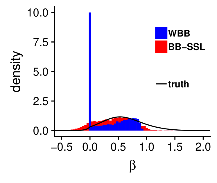
(a) $y_{i}=1$

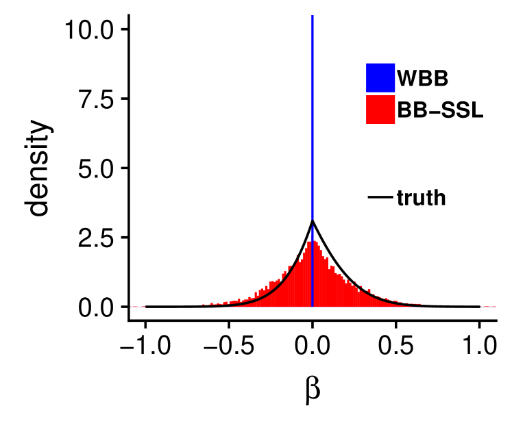
(b) $y_{i}=0.1$

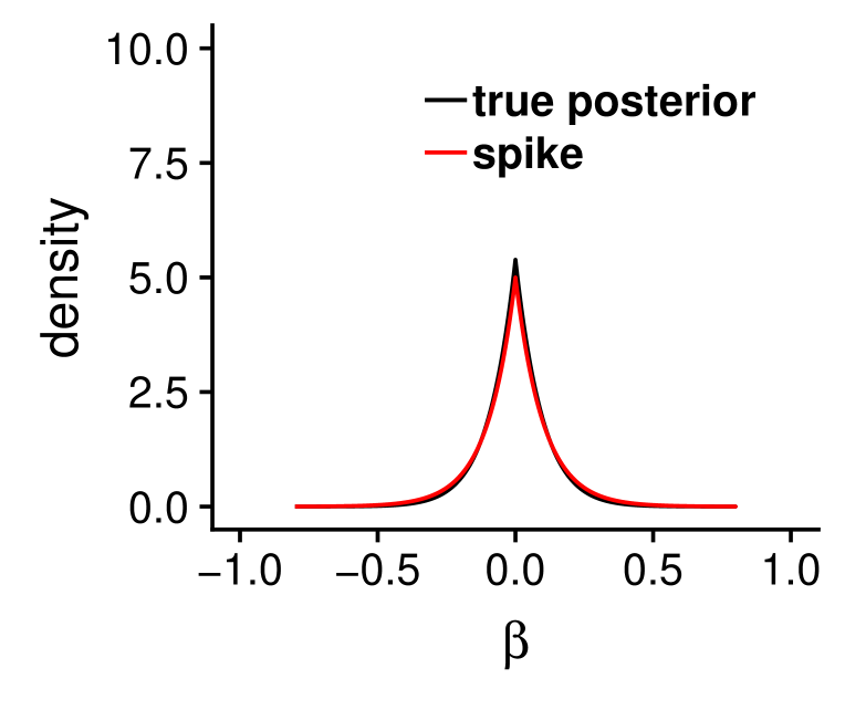
(c) True posterior versus spike.

Figure 1: True and WBB approximated posterior distribution $\pi(\beta_{i}\,|\>y_{i})$ under the separable SSL prior with $\lambda_{0}=5,\lambda_{1}=0.1$ and $\theta=0.2$ and a Gaussian sequence model $y_{i}=x_{i}+\epsilon_{i}/\sqrt{n}$ with $n=10$. Red bins represent BB-SSL pseudo-posterior, blue bins represent WBB pseudo-posterior (with a random prior weight), black line is the true posterior and $\alpha=2.5$. The plot (c) is for the same setting except with $\lambda_{0}=10$.

Intuitively, $\lambda_{1}/n$ vanishes when $n$ is large, so both $\phi_{1}^{(-)}(\beta_{i})$ and $\phi_{1}^{(+)}(\beta_{i})$ will be close to $\phi(\beta_{i};y_{i},\frac{1}{n})$. This intuition is proved rigorously in the Appendix (Section A.6.2), where we show that the density of the transformed variable $\sqrt{n}(\beta_{i}-y_{i})$ converges pointwise to the standard normal density and thereby the posterior $\pi\left(\sqrt{n}(\beta_{i}-y_{i})\,|\>y_{i},\gamma_{i}=1\right)$ converges to $N(0,1)$ in total variation (Scheffé (1947)).

We now investigate the limiting shape of the pseudo-distribution obtained from WBB. For a given weight $w_{i}>0$, the WBB estimator $\smash{\widehat{\beta}}_{i}$ equals

$$\smash{\widehat{\beta_{i}}}=\begin{cases}0,&\text{if $|y_{i}|\leq{\Delta_{w_{i}}}$}.\\ \left[|y_{i}|-\frac{1}{w_{i}n}\lambda^{*}(\smash{\widehat{\beta_{i}}})\right]_{+}\mathrm{sign}(\sqrt{w_{i}n}y_{i}),&\text{otherwise}.\end{cases}$$ (11)

where $\Delta_{w_{i}}=\inf_{t>0}[t/2-\rho(t\,|\>\theta)/(nw_{i}t)]$ is the analogue of $\Delta_{j}$ defined below (4) for the regression model and where $\rho(t\,|\>\theta)$ was also defined below (4). When $\smash{\widehat{\beta}}_{i}\neq 0$, we show in the Appendix (Section A.6.2) that $n\left(\smash{\widehat{\beta_{i}}}-y_{i}\right)\rightarrow-\frac{1}{w_{i}}\lambda_{1}$. Under the condition $|y_{i}|>\frac{|\beta_{i}^{0}|}{2}>0$, it can be shown (Section A.6.2) that $\mathbb{P}_{w_{i}}\left(\smash{\widehat{\beta}}_{i}=0\,|\>y_{i}\right)\rightarrow 0$. For active coordinates, the distribution of the WBB samples $\smash{\widehat{\beta}}_{i}$ is thus purely determined by that of $-\frac{1}{w_{i}}$. The shape of this posterior can be very different from the standard normal one, as can be seen from Figure 1. In particular, Figure 1(a) shows how WBB (a) assigns a non-negligible prior mass to zero (in spite of evidence of signal) (b) incurs bias in estimation and (c) underestimates variance with a skewed misrepresentation of the posterior distribution. This last aspect is particularly pronounced when the signal is even stronger.

The approximability of WBB does not get any better for inactive coordinates such that $\beta_{i}^{0}=0$ and thereby $|y_{i}|=O_{p}(\frac{1}{\sqrt{n}})$ from (7). The following arguments will be under the assumption $|y_{i}|\asymp\frac{1}{\sqrt{n}}$. One can show (Section A.6.3 in the Appendix) that the true posterior $\pi\left(\beta_{i}\,|\>y_{i}\right)$ is dominated by the component $\pi\left(\beta_{i}\,|\>y_{i},\gamma_{i}=0\right)$ since $w_{0}\rightarrow 1$ and $w_{1}\rightarrow 0$. When $n$ is sufficiently large, one can then approximate this distribution with the Laplace spike, indeed $\pi\left(\lambda_{0}\beta_{i}\,|\>y_{i},\gamma_{i}=0\right)$ converges to $\frac{1}{2}e^{-|\lambda_{0}\beta_{i}|}$ in total variation (Section A.6.3 in the Appendix). When the signal is weak, the posterior thus closely resembles the spike Laplace distribution, as can be seen from Figure 1(c). For the fixed (and also random) WBB pseudo-posteriors, we show (in Section A.6.3 in the Appendix) that the posterior converges to a point mass at 0, i.e. $\mathbb{P}_{w_{i}}\left(\smash{\widehat{\beta}}_{i}=0\,|\>y_{i}\right)\rightarrow 1.$ This is a misleading approximation of the actual posterior (Figure 1(b)). To conclude, since SSL is always shrinking the estimates towards $0$, WBB samples will often be zero. The true posterior, however, follows roughly a spike Laplace distribution when the signal is weak. Motivated by Papandreou and Yuille (2010), one possible solution is to introduce randomness in the shrinkage target of the prior.

4 Introducing BB-SSL

Similarly as Newton et al. (2020), we argue that the random perturbation should affect both the prior and the data. Instead of inflating the prior contribution by a fixed or random weight, we perturb the prior mean for each coordinate. This creates a random shift in the centering of the prior so that the posterior can shrink to a random location as opposed to zero. Instead of the prior $\pi(\boldsymbol{\beta}\,|\>\boldsymbol{\gamma})$ in (2) which is centered around zero, we consider a variant that uses hierarchical jittered Laplace distributions.

Definition 4.1.

For $\lambda_{0}\gg\lambda_{1}$, a location shift vector $\boldsymbol{\mu}=(\mu_{1},\mu_{2},\cdots,\mu_{p})^{T}\in\mathbb{R}^{p}$ and a prior inclusion weight $\theta\in(0,1)$, the jittered Spike-and-Slab LASSO prior is defined as

$$\widetilde{\pi}(\boldsymbol{\beta}\,|\>\boldsymbol{\mu},\theta)=\prod_{i=1}^{p}[\theta\psi_{1}(\beta_{i};\mu_{i})+(1-\theta)\psi_{0}(\beta_{i};\mu_{i})],\quad\text{where}\quad\mu_{i}\stackrel{{\scriptstyle iid}}{{\sim}}\psi_{0}(\mu)$$ (12)

and where $\psi_{1}(\beta;\mu)=\lambda_{1}/2\mathrm{e}^{-|\beta-\mu|\lambda_{1}}$, $\psi_{0}(\beta;\mu)=\lambda_{0}/2\mathrm{e}^{-|\beta-\mu|\lambda_{0}}$ and $\psi_{0}(\beta)=\psi_{0}(\beta;0)$.

Set: $\lambda_{0}\gg\lambda_{1},$ $a,b>0$ and $T$ (number of iterations).

for $t=1,2,\cdots,T$ do

                                                   ahoj

       (a) Sample $\boldsymbol{w}_{t}\sim\pi(\boldsymbol{w})$.

       (b) Sample $\boldsymbol{\mu}_{t}$ from $\mu^{t}_{j}\stackrel{{\scriptstyle iid}}{{\sim}}\psi_{0}(\mu)$.

       (c) Calculate $\widetilde{\boldsymbol{\beta}}_{t}$ from (13).

end for

Algorithm 2 : BB-SSL Sampling

The Bayesian Bootstrap Spike-and-Slab LASSO (which we abbreviate as BB-SSL) is obtained by maximizing a pseudo-posterior obtained by reweighting the likelihood and recentering the prior. Namely, one first samples weights $w_{i}^{t}$, one for each observation, from $\boldsymbol{w}_{t}=(w_{1}^{t},\dots,w_{n}^{t})^{T}\sim n\,\mathrm{Dirichlet}(\alpha,\cdots,\alpha)$ for some $\alpha>0$ (we discuss choices in the next section). Second, one samples the location shifts $\boldsymbol{\mu}_{t}=(\mu_{1}^{t},\dots,\mu_{p}^{t})^{T}$ from the spike distribution as in (12). Lastly, a draw $\widetilde{\boldsymbol{\beta}}_{t}$ from the BB-SSL posterior is obtained as a pseudo-MAP estimator

$$\widetilde{\boldsymbol{\beta}}_{t}=\arg\max_{\boldsymbol{\beta}\in\mathbb{R}^{p}}\left\{\widetilde{L}^{\boldsymbol{w}_{t}}(\boldsymbol{\beta},\sigma^{2};\boldsymbol{X}^{(n)},\boldsymbol{Y}^{(n)})\times\int_{\theta}\widetilde{\pi}(\boldsymbol{\beta}\,|\>\boldsymbol{\mu}_{t},\theta)d\pi(\theta)\right\}.$$ (13)

BB-SSL can be implemented by directly applying the SSL algorithm we described in the previous section on randomly perturbed data. In particular, denote with $\boldsymbol{\beta}^{*}=\boldsymbol{\beta}-\boldsymbol{\mu}_{t},\,Y_{i}^{*}=\sqrt{w_{i}^{t}}\left(Y_{i}-\boldsymbol{x}_{i}^{T}\boldsymbol{\mu}_{t}\right),\,\boldsymbol{x}_{i}^{*}=\sqrt{w_{i}^{t}}\boldsymbol{x}_{i}$. We can first calculate

$$\smash{\widehat{\boldsymbol{\beta}_{t}^{*}}}=\arg\max_{\boldsymbol{\beta}\in\mathbb{R}^{p}}\left\{\widetilde{L}^{\boldsymbol{w}_{t}=(1,1,\cdots,1)}(\boldsymbol{\beta}^{*},\sigma^{2};\boldsymbol{X}^{*},\boldsymbol{Y}^{*})\times\int_{\theta}\widetilde{\pi}(\boldsymbol{\beta}\,|\>\boldsymbol{0},\theta)d\pi(\theta)\right\},$$

and then get $\widetilde{\boldsymbol{\beta}}_{t}$ through a post-processing step $\widetilde{\boldsymbol{\beta}}_{t}=\smash{\widehat{\boldsymbol{\beta}^{*}_{t}}}+\boldsymbol{\mu}_{t}.$

4.1 Theory for BB-SSL

For the uniform Dirichlet weights, Newton and Raftery (1994) (Theorem 1 and 2) show first-order correctness, i.e. consistency and asymptotic normality, of WLB in low dimensional settings (a fixed number of parameters) and iid observations. Their result can be generalized to WBB (Newton et al., 2020; Ng and Newton, 2020) as well as BB-SSL. While the uniform Dirichlet weight distribution is a natural choice, Newton and Raftery (1994) point out that it is doubtful that such weights would yield good higher-order approximation properties. The authors leave open the question of relating the weighting distribution to the model itself and to a more general prior. A more recent theoretical development in this direction is the work of Ng and Newton (2020) who find that WBB first-order correctness holds for a wide class of random weight distributions in low-dimensional LASSO regressions. They also theoretically assess the influence of assigning random weights to the penalty term. Here, we address this question by looking into asymptotics for guidance about the weight distribution. We focus on high-dimensional scenarios where the number of parameters ultimately increases with the sample size.

In particular, we provide sufficient conditions for the weight distribution $\pi(\boldsymbol{w})$ so that the pseudo-posterior concentrates at the same rate as the actual posterior under the same prior settings. After stating the result for general weight distributions, we particularize our considerations to Dirichlet and gamma distributions and provide specific guidance for implementation. Our first result is obtained for the canonical high-dimensional normal-means problem, where $\boldsymbol{Y}^{(n)}=(Y_{1},\dots,Y_{n})^{T}$ is observed as a noisy version of a sparse mean vector $\boldsymbol{\beta}_{0}=(\beta_{1}^{0},\dots,\beta_{n}^{0})^{T}$, i.e.

$$Y_{i}=\beta^{0}_{i}+\epsilon_{i},\quad\text{where}\quad\epsilon_{i}\stackrel{{\scriptstyle iid}}{{\sim}}\mathcal{N}(0,{\sigma^{2}})\quad\text{for $1\leq i\leq n$}.$$ (14)

Theorem 4.1 (Normal Means).

Consider the normal means model (14) with $q=\|\boldsymbol{\beta}_{0}\|_{0}$ such that $q=o(n)$ as $n\rightarrow\infty$. Assume the SSL prior with $0<\lambda_{1}<\frac{1}{e^{2}}$ and $\theta\asymp(\frac{q}{n})^{\eta},\lambda_{0}\asymp(\frac{n}{q})^{\gamma}$ with $\eta,\gamma>0$ such that $\eta+\gamma>1$. Assume that $\boldsymbol{w}=(w_{1},\dots,w_{n})^{T}$ are non-negative and arise from $\pi(\boldsymbol{w})$ such that

1. $\mathbb{E}\,w_{i}=1$ for each $1\leq i\leq n$,

2. $\exists\,C_{1},C_{2}>0$ such that $\mathbb{E}\left(\frac{1}{w_{i}}\right)\leq C_{1}$ and $\mathbb{E}\left(\frac{1}{w_{i}^{2}}\right)\leq C_{2}$ for each $1\leq i\leq n$,

3. $\exists\,C_{3}>0$ such that for each $1\leq i\leq n$

   $$\mathbb{P}(w_{i}>\eta+\gamma)\leq C_{3}\,\frac{q}{n}\,\sqrt{\log\left(\frac{n}{q}\right)}.$$

Then, for any $M_{n}\rightarrow\infty$, the BB-SSL posterior concentrates at the minimax rate, i.e.

$$\lim_{n\rightarrow\infty}\mathbb{E}_{\boldsymbol{\beta}_{0}}\mathbb{P}_{\boldsymbol{w},\boldsymbol{\mu}}\left[\|\widetilde{\boldsymbol{\beta}}_{\boldsymbol{w}}^{\boldsymbol{\mu}}-\boldsymbol{\beta}_{0}\|_{2}^{2}>M_{n}\,q\log\left(\frac{n}{q}\right)\,|\>\boldsymbol{Y}^{(n)}\right]=0.$$ (15)

Proof.

See Section A.1.2 in the Appendix.

In Theorem 4.1, $\widetilde{\boldsymbol{\beta}}_{\boldsymbol{w}}^{\boldsymbol{\mu}}$ denotes the BB-SSL sample whose distribution, for each given $\boldsymbol{Y}^{(n)}$, is induced by random weights $\boldsymbol{w}$ arising from $\pi(\boldsymbol{w})$ and random recentering $\boldsymbol{\mu}$ arising from $\psi_{0}(\cdot)$. Despite the approximate nature of BB-SSL, the concentration rate (15) is minimax optimal and it is the same rate achieved by the actual posterior distribution under the same prior assumptions (Ročková (2018a)). Condition (1) in Theorem 4.1 is not surprising and aligns with considerations in Newton et al. (2020). Conditions (2) and (3) can be viewed as regularizing the tail behavior of $w_{i}$’s (left and right, respectively). While Newton et al. (2020) only showed consistency for iid models in finite-dimensional settings, Theorem 4.1 is far stronger as it shows optimal convergence rate in a high-dimensional scenario. The following Corollary discusses specific choices of $\pi(\boldsymbol{w})$.

Corollary 4.1.

Assume the same model and prior as in Theorem 4.1. Next, when $\boldsymbol{w}=(w_{1},w_{2},\cdots,w_{n})^{T}\sim n\times\mathrm{Dir}(\alpha,\alpha,\cdots,\alpha)$ with $\alpha\gtrsim\sigma^{2}\log[\frac{(1-\theta)\lambda_{0}}{\theta\lambda_{1}}]$ or $w_{i}\overset{\text{i.i.d}}{\sim}\frac{1}{\alpha}Gamma(\alpha,1)$ with $\alpha\gtrsim\sigma^{2}\log\left[\frac{(1-\theta)\lambda_{0}}{\theta\lambda_{1}}\right]$, the BB-SSL posterior satisfies (15).

Proof.

See the Appendix (Section A.2).

Theorem 4.1 and Corollary 4.1 give insights into what weight distributions are appropriate for sparse normal means. In parametric models, the uniform Dirichlet distribution would be enough to achieve consistency (Newton and Raftery, 1994). It is interesting to note, however, that in the non-parametric normal means model, the assumption $\boldsymbol{w}\sim n\times\mathrm{Dir}(\alpha,\cdots,\alpha)$ for $\alpha<2$ yields risk (for active coordinates) that can be arbitrarily large (as we show in Section A.3 in the Appendix). The requirement $\alpha\geq 2$ is thus necessary for controlling the risk of active coordinates and the plain uniform Dirichlet prior (with $\alpha=1$) would not be appropriate.

In the following theorems, we study the high-dimensional regression model (1) with rescaled columns $\|\boldsymbol{X}_{j}\|_{2}=\sqrt{n}$ for all $j=1,2,\cdots,p$.

Theorem 4.2 (Regression Model Size).

Consider the regression model (1) with $p>n$, $q=\|\boldsymbol{\beta}\|_{0}$ (unknown). Assume the SSL prior with $(1-\theta)/\theta\asymp p^{\eta}$ and $\lambda_{0}\asymp p^{\gamma}$ where $\eta,\gamma\geq 1$. Assume that $\boldsymbol{w}=(w_{1},\cdots,w_{n})^{T}$ are non-negative and arise from $\pi(\boldsymbol{w})$ such that

1. $\mathbb{E}\,w_{i}=1$ for each $1\leq i\leq n$,

2. $\exists\,m\in(0,1)\,\,\text{s.t.}\,\,\lim_{n\rightarrow\infty}\mathbb{P}(\min_{i}w_{i}>m)=1$,

3. $\exists\,M>1\,\,\text{s.t.}\,\,\lim_{n\rightarrow\infty}\mathbb{P}(\max_{i}w_{i}<M)=1$,

4. $Var(w_{i})\lesssim\frac{1}{\log n},\,Cov(w_{i},w_{j})=C_{0}\lesssim\frac{1}{n\log n}$ for any $1\leq i,j\leq n$,

5. $\max_{i\neq j}|\boldsymbol{x}_{i}^{T}\boldsymbol{x}_{j}|\lesssim\lambda_{0}^{2}/n$, and $\xi_{0}>0$ satisfies

   $$\begin{split}\max\{&\lambda_{\text{max}}^{1/2}\left(\boldsymbol{X}_{B}^{T}\boldsymbol{P}_{A}\boldsymbol{X}_{B}/n\right):B\cap A=\emptyset,|A|=rank(P_{A})=|B|=k,\,\\ &k(1+\xi_{0})^{2}\left(1+\sqrt{2.5\log p}\right)^{2}\leq 2n\}\leq\xi_{0}.\end{split}$$

6. $D=\frac{M}{m}\left(\frac{\eta^{*}}{c}+\frac{d\lambda_{1}}{\sqrt{n\log p}}\right)^{2}<1-\delta$ for some $\delta>0$, where $\eta^{*}=\max\left\{\widetilde{\eta}+C_{n}\frac{\|\boldsymbol{X}\|}{\lambda_{1}},\frac{\widetilde{\eta}}{m}\right\}\in(0,1)$, $\widetilde{\eta}>\frac{\sqrt{5}}{2\sqrt{\eta+\gamma}}(1+\xi_{0})$, $C_{n}$ is a sequence s.t. $C_{n}\rightarrow\infty$, $d=\frac{\sigma}{c\sqrt{2(\eta+\gamma-1)}}$ and $c=c(\eta^{*};\boldsymbol{\beta})$.

Then the BB-SSL posterior satisfies

$$\lim_{n\rightarrow\infty}\mathbb{E}_{\boldsymbol{\beta}_{0}}\mathbb{P}_{\boldsymbol{\mu},\,\boldsymbol{w}}\left(\|\widetilde{\boldsymbol{\beta}}_{\boldsymbol{w}}^{\boldsymbol{\mu}}-\boldsymbol{\mu}\|_{0}\leq q(1+K)\,|\>\boldsymbol{Y}^{(n)}\right)=1$$

where $K=2\frac{D}{1-D}$. The definition of $c(\eta^{*};\boldsymbol{\beta})$ is in the Appendix, Section A.4.1.

Proof.

Section A.4.6 in the Appendix.

Theorem 4.3 (Regression model).

Under the same conditions as in Theorem 4.2, the BB-SSL posterior concentrates at the near-minimax rate, i.e.,

$$\lim_{n\rightarrow\infty}\mathbb{E}_{\boldsymbol{\beta}_{0}}\mathbb{P}_{\boldsymbol{w},\,\boldsymbol{\mu}}\left(\|{\widetilde{\boldsymbol{\beta}}}_{\boldsymbol{w}}^{\boldsymbol{\mu}}-\boldsymbol{\beta}_{0}\|_{2}^{2}>\frac{C_{5}(\eta^{*})^{2}{M}}{m\,\phi^{2}\,c^{2}}q(1+K)\frac{\log p}{n}\,|\>\boldsymbol{Y}^{(n)}\right)=0$$ (16)

where $c=c(\eta^{*};\boldsymbol{\beta}),\phi=\phi\left(C(\eta^{*};\boldsymbol{\beta}_{0})\right)$, whose definition are in the Appendix A.4.1.

Proof.

Section A.4.7 in the Appendix.

It follows from Ročková and George (2018) and from (16) that the BB-SSL posterior achieves the same rate of posterior concentration as the actual posterior. In Theorem 4.2, Conditions (1)-(4) regulate the distribution $\pi(\boldsymbol{w})$ while Conditions (5) and (6) impose requirements on $\boldsymbol{X}$, $\lambda_{0}$ and $\lambda_{1}$. Conditions (2) and (3) are counterparts of (2) and (3) in Theorem 4.1 and control the left and right tail of $w_{i}$’s, respectively. The larger $M$ (or the smaller $m$) is, the larger $D$ and $K$ will become and the larger the bound on $\|{\widetilde{\boldsymbol{\beta}}}_{\boldsymbol{w}}^{\boldsymbol{\mu}}-\boldsymbol{\beta}_{0}\|_{2}^{2}$ will be. Compared with the normal means model, we have one additional Condition (4) which requires that each $w_{i}$ becomes more and more concentrated around its mean and that $w_{i}$’s are asymptotically uncorrelated. It is interesting to note that distributions $\pi(\boldsymbol{w})$ in Corollary 4.1 both satisfy Condition (4). Moreover, the Dirichlet distribution in Corollary 4.1 achieves both upper bounds tightly. Finally, Condition (5) ensures that identifiability holds with high probability (Zhang and Zhang (2012)) and Condition (6) ensures that our bound is meaningful. In practice, many distributions will satisfy Conditions (1)-(4), e.g. bounded distributions with a proper covariance structure or distributions from Corollary 4.1.

Remark 4.1.

In the regression model, when $\boldsymbol{w}$ arises from the same distribution as in Corollary 4.1, Conditions (1)-(4) in Theorem 4.3 are satisfied by setting $m=\frac{1}{e}$ and $M=\frac{2}{3}(\eta+\gamma)$. The detailed proof is in Section A.5 in the Appendix.

Data: Data ($Y_{i}$, $\boldsymbol{x}_{i}$) for $1\leq i\leq n,x_{i}\in\mathbb{R}^{p}$, truncation limit $m$

Result: $\tilde{\boldsymbol{\beta}}^{t},t=1,2,\cdots,T$

for $t=1,2,\cdots,T$ do

                                                   ahoj

       (a) Draw prior pseudo-samples $\tilde{\boldsymbol{x}}_{1:m},\tilde{y}_{1:m}\sim F_{\pi}$.

       (b) Draw $(w_{1:n},\tilde{w}_{1:m})$ $\sim\text{Dir}(1,1,\cdots,1,c/m,c/m,\cdots,c/m)$.

       (c) Calculate $\widetilde{\boldsymbol{\beta}}^{t}=\arg\max_{\boldsymbol{\beta}\in\mathbb{R}^{p}}\left\{\sum_{j=1}^{n}w_{j}l(\boldsymbol{x}_{j},y_{j},\boldsymbol{\beta})+\sum_{k=1}^{m}\tilde{w}_{k}l(\tilde{\boldsymbol{x}}_{k},\tilde{y}_{k},\boldsymbol{\beta})\right\}$.

end for

Algorithm 3 : Posterior Bootstrap Sampling

4.2 Connections to Other Bootstrap Approaches

Our approach bears a resemblance to Bayesian non-parametric learning (NPL) introduced by Lyddon et al. (2018) and Fong et al. (2019) which generates exact posterior samples under a Bayesian non-parametric model that assumes less about the underlying model structure. Under a prior on the sampling distribution function $F_{\pi}$, one can use WBB (and also WLB) to draw samples from a posterior of $F_{\pi}$ by optimizing a randomly weighted loss function $l(\cdot)$ based on an enlarged sample (observed plus pseudo-samples) with weights following a Dirichlet distribution (see Algorithm 3 which follows from Fong et al. (2019)). Despite the fact that these two procedures have different objectives, there are many interesting connections. In particular, the idea of randomly perturbing the prior has an effect similar to adding pseudo-samples $\widetilde{\boldsymbol{x}}_{1:m},\widetilde{y}_{1:m}$ from the prior $F_{\pi}(\boldsymbol{x},y)$ defined through

$$\widetilde{\boldsymbol{x}}_{k}\sim F_{n}(\boldsymbol{x})=\frac{1}{n}\sum_{i=1}^{n}\delta(\boldsymbol{x}_{i}),\quad\widetilde{y}_{k}\,|\>\widetilde{\boldsymbol{x}}_{k}=\smash{\widehat{y}}_{k}+\widetilde{\boldsymbol{x}}_{k}^{T}\boldsymbol{\mu}$$

where $\delta(\cdot)$ is the Dirac measure, $\boldsymbol{\mu}$ is the Spike, and $\smash{\widehat{y}}_{k}=y_{i}$ where $i$ satisfies $\widetilde{\boldsymbol{x}}_{k}=\boldsymbol{x}_{i}$. A motivation for this prior is derived in the Appendix (Section B). Under this prior, the NPL posterior samples $\widetilde{\boldsymbol{\beta}}^{t}$ generated by Algorithm 3 approximately follow the distribution (see Section B in the Appendix)

$$\widetilde{\boldsymbol{\beta}}^{t}\text{$\overset{\text{d}}{\approx}$}\arg\max_{\widetilde{\boldsymbol{\beta}}\in\mathbb{R}^{p}}\left\{-\frac{1}{2}\sum_{i=1}^{n}w_{i}^{*}(Y_{i}-\boldsymbol{x}_{i}^{T}\tilde{\boldsymbol{\beta}})^{2}+\log\left[\int\prod_{j=1}^{p}\pi\left(\tilde{\beta}_{j}-\frac{c}{c+n}\mu_{j}^{*}\,|\>\theta\right)d\pi(\theta)\right]\right\}-\frac{c}{c+n}\boldsymbol{\mu}^{*}$$ (17)

where $(w_{1}^{*},w_{2}^{*},\cdots,w_{n}^{*})^{T}\sim n\times\text{Dir}(1+c/n,\cdots,1+c/n)$, each coordinate of $\boldsymbol{\mu}^{*}$ independently follows the spike distribution, and where $c$ represents the strength of our belief in $F_{\pi}$ and can be interpreted as the effective sample size from $F_{\pi}$. In comparison with the BB-SSL estimate

$$\widetilde{\boldsymbol{\beta}}^{t}=\arg\max_{\widetilde{\boldsymbol{\beta}}\in\mathbb{R}^{p}}\left\{-\frac{1}{2}\sum_{i=1}^{n}w_{i}(Y_{i}-\boldsymbol{x}_{i}^{T}\widetilde{\boldsymbol{\beta}})^{2}+\log\left[\int_{\theta}\prod_{j=1}^{p}\pi\left(\tilde{\beta}_{j}-\mu_{j}\,|\>\theta\right)d\pi(\theta)\right]\right\}$$ (18)

where $(w_{1},w_{2},\cdots,w_{n})^{T}\sim n\times\text{Dir}(\alpha,\cdots,\alpha)$, both (17) and (18) are shrinking towards a random location and both are using Dirichlet weights. The main difference is in the choice of the concentration parameter $c$. When $c=0$, (17) reduces to WBB (with a fixed weight on the prior) which reflects less confidence in the prior $F_{\pi}$ and thus less prior perturbation (location shift). When $c$ is large, (17) becomes more similar to (18) where the prior $F_{\pi}$ is stronger and thereby more prior perturbation is induced. Another difference is that (17), although shrinking towards a random location $\frac{c}{c+n}\mu_{j}^{*}$, adds the location back which results in less variance (see Figures in Section B in the Appendix).

Algorithm	Complexity
SSVS1	$O(p^{2}n)$
SSVS2	$O(n^{2}\max(p,n))$
Skinny Gibbs	$O(np)$
WLB	$O(np^{2})$ when $n\leq p$, not applicable when $p>n$
BB-SSL	$O\left(\min\left(\text{maxiter}\times p(n+\frac{p}{c_{1}}),\,(n+\text{maxiter})\times p^{2}\right)\right)$ for a single value $\lambda_{0}$

Table 1: A computational complexity analysis (per sample) of each algorithm. Maxiter is the user-specified maximum number of iterations with a default value $500$. For BB-SSL, $c_{1}$ is the pre-specified number of iterations after which $\theta$ is updated with a default value $10$. By setting $c_{1}\propto p$ we have BB-SSL complexity $O(np)$.

5 Simulations

We compare the empirical performance of our BB-SSL with several existing posterior sampling methods including WBB (Newton et al. (2020)), SSVS (George and McCulloch (1993)), and Skinny Gibbs (Narisetty et al. (2019)). We implement two versions of WBB: WBB1 (with a fixed prior weight) and WBB2 (with a random prior weight). We also implement the original SSVS algorithm (Algorithm 1 further referred to as SSVS1) and compare its complexity and running times with its faster version (further referred to as SSVS2) which uses the trick from Bhattacharya et al. (2016). Comparisons are based on the marginal posterior distributions for $\beta_{i}$’s, marginal inclusion probabilities (MIP) $\mathbb{P}(\gamma_{i}=1\,|\>\boldsymbol{Y}^{(n)})$ as well as the joint posterior distribution $\pi(\boldsymbol{\gamma}\,|\>\boldsymbol{Y}^{(n)})$. As the benchmark gold standard for comparisons, we run SSVS initialized at the truth for a sufficiently large number of iterations $T$ and discard the first $B$ samples as a burn-in. We use the same $T$ and $B$ for Skinny Gibbs except that we initialize $\boldsymbol{\beta}$ at the origin. For BB-SSL, we draw weights $\boldsymbol{w}\sim n\times\text{Dir}(\alpha,\cdots,\alpha)$ where $\alpha$ depends on $(n,p,\sigma^{2})^{T}$. When solving the optimization problem (13) using coordinate-ascent, the default initialization for $\boldsymbol{\beta}$ in the SSLASSO R package (Ročková and Moran, 2017) is at the origin. In high-dimensional correlated settings when $\lambda_{0}>>\lambda_{1}$, however, the performance of BB-SSL can be further enhanced by using a warm start re-initialization strategy for a sequence of increasing $\lambda_{0}$’s where the last value is the target $\lambda_{0}$ value (as recommended by Ročková (2018a) and Ročková and Moran (2017)). It is computationally more economical to perform such annealing only once on the original data and then use the output (for the target value $\lambda_{0}$) for each BB-SSL iteration. We apply this strategy using an output obtained from the R package SSLASSO using an equispaced sequence of $\lambda_{0}$’s of length $50$, starting at $\lambda_{1}$ and ending at $\lambda_{0}$. We then run WWB1, WBB2 and BB-SSL for $T$ iterations. Throughout the simulations we set $\sigma^{2}=1$ and assume the prior $\theta\sim B(1,p)$. Computational complexity of each algorithm is summarized in Table 1 with actual running times reported (for varying $p$ and $n$) in Figure 2.

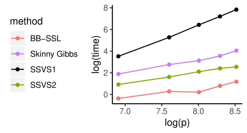
(a) $n=100$.

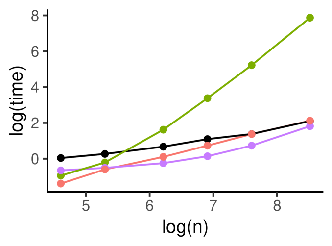
(b) $p=100$.

Figure 2: Average running times (in seconds on a log scale) for $100$ iterations of each algorithm based $10$ independent runs. Covariates are all correlated with a correlation coefficient $\rho=0.6$. Signals are $(2,3,-3,4)$ and we set $\lambda_{0}=200,\lambda_{1}=0.05,a=1,b=p$. BB-SSL is initialized at the SS-LASSO solution obtained with a sequence of $\lambda_{0}$’s (an equi-spaced series of length $50$ starting at $\lambda_{1}=0.05$ and ending at $\lambda_{0}=200$).

5.1 The Low-dimensional Case

Similarly to the experimental setting in Ročková (2018b), we generate $n=50$ observations on $p=12$ predictors with $\boldsymbol{\beta}_{0}=(1.3,0,0,1.3,0,0,1.3,0,0,1.3,0,0)^{T}$, where the predictors have been grouped into $4$ blocks. Within each block, predictors have an equal correlation $\rho$ and there is only one active predictor. All the other correlations are set to 0. We choose a single value for $\lambda_{0}\propto p$ and generate Dirichlet weights assuming $\alpha=1$ (for WBB1, WBB2 and BB-SSL).

Uncorrelated Designs

Assuming $\rho=0,\lambda_{0}=12$ and $\lambda_{1}=0.05$ we run SSVS1 and Skinny Gibbs for $T=10\,000$ iterations with a burn-in $B=5\,000$. For WBB1, WBB2 and BB-SSL we use $T=5\,000$ iterations. All methods perform very well under various metrics in this setting. We refer the reader to Section E.1 in the Appendix for details.

Correlated Designs

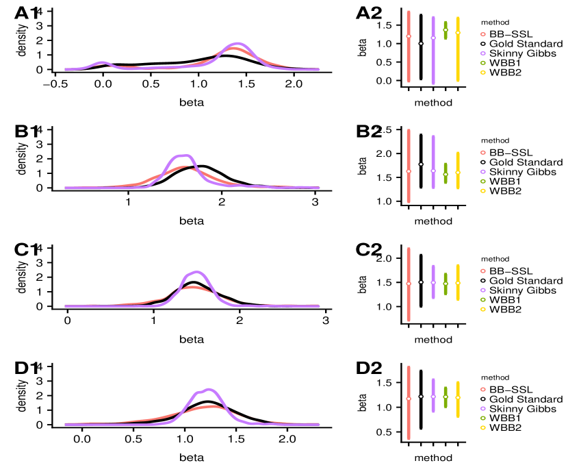
(a) Active predictors, from top to bottom: $\beta_{1},\beta_{4},\beta_{7},\beta_{10}$

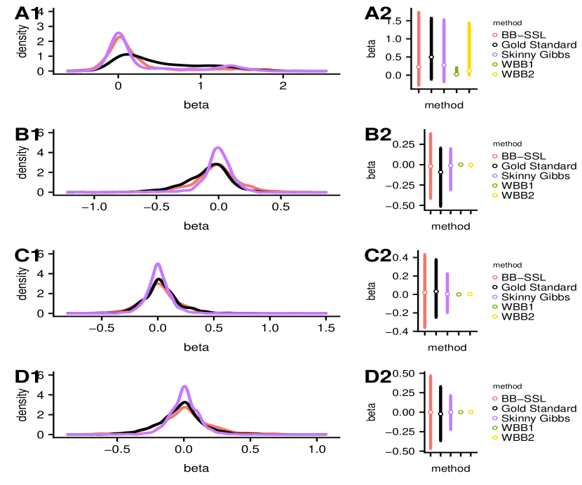
(b) Inactive predictors, from top to bottom: $\beta_{2},\beta_{5},\beta_{8},\beta_{11}$

Figure 3: Estimated posterior density (left panel) and credible intervals (right panel) of $\beta_{i}$’s in the low-dimensional correlated case. We have $n=50,p=12,\beta_{active}=(1.3,1.3,1.3,1.3)^{\prime},\lambda_{0}=7,\lambda_{1}=0.15,\rho=0.9$. Each method has $5\,000$ sample points (after thinning for SSVS and Skinny Gibbs). BB-SSL is fitted using a single value $\lambda_{0}=7$. Since WBB1 and WBB2 produce a point mass at zero, we exclude them from density comparisons.

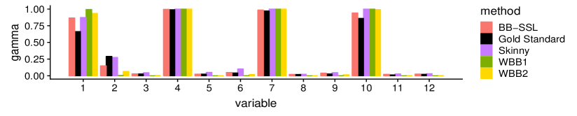
(a) Marginal inclusion probability.

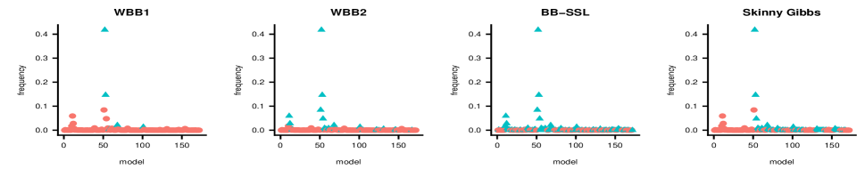
(b) Posterior exploration plot. Blue (red) triangles are visited (unvisited) models.

Figure 4: The low-dimensional correlated case with $n=50,p=12,\beta_{active}=(1.3,1.3,1.3,1.3)^{\prime}$ where predictors are grouped into $4$ correlated blocks with $\rho=0.9$. We choose $\lambda_{0}=7,\lambda_{1}=0.15$.

Correlated designs are far more interesting for comparisons. We choose $\rho=0.9,\lambda_{0}=7$ and $\lambda_{1}=0.15$ to deliberately encourage multimodality in the model posterior (see Figure 4(b)). For SSVS1 and Skinny Gibbs, we set $T=100\,000$ and $B=5\,000$. For WBB1, WBB2 and BB-SSL we set $T=95\,000$.

In terms of the marginal densities of $\beta_{i}$’s, Figure 3 shows that BB-SSL tracks SSVS1 very closely. All methods can cope with multi-collinearity where BB-SSL tends to have slightly longer credible intervals with the opposite being true for Skinny Gibbs, WBB1 and WWB2. In terms of the marginal means of $\gamma_{i}$ (Figure 4(a)) all methods perform well, where the median probability model rule (truncating the marginal means at 0.5) yields the true model. In terms of the overall posterior $\pi(\boldsymbol{\gamma}\,|\>\boldsymbol{Y}^{(n)})$, we identify over 60 unique models using SSVS1 where the true model accounts for most of the posterior mass. In Figure 4(b), we show the visited (blue triangle) and not visited (red dots) among these models, where $y$-axis represents the estimated posterior probability for each model (calculated from SSVS1). All methods can detect the dominating model. BB-SSL tracked down 99% of the posterior probability, followed by WBB1 (92%), WBB2 (91%) and Skinny Gibbs (73%). The average times (reported in seconds and ordered from fastest to slowest) spent on generating $1\,000$ effective samples for $\beta_{j}$’s are WBB2 (0.68 s) $<$ WBB1 (0.72 s) $<$ BB-SSL (0.74 s) $<$ SSVS2 (0.82 s) $<$ SSVS1 (0.85 s) $<$ Skinny Gibbs (1.19 s).

5.2 The High-dimensional Case

We now consider a higher-dimensional case with $n=100$ and $p=1\,000$, assuming $\lambda_{0}=50,\lambda_{1}=0.05$ and $\alpha=2$ for BB-SSL. For SSVS1 and Skinny Gibbs we set $T=15\,000$ and $B=5\,000$ while for WBB1, WBB2 and BB-SSL we set $T=1\,000$.

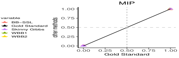
(a) $\rho=0$

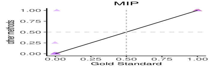
(b) block-wise $\rho=0.9$

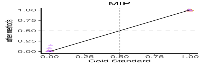
(c) equi-correlation $\rho=0.6$

Figure 5: Posterior means of $\gamma_{i}$’s (i.e. a marginal inclusion probabilities) in high-dimensional settings with $n=100,p=1000$. We set $\lambda_{0}=50,\lambda_{1}=0.05$.

We consider two correlation structures: (a) block-wise correlation, and (b) equi-correlation. In the setting (a), the active predictors have regression coefficients $(1,2,-2,3)^{T}$ and all predictors are grouped into blocks of size $10$, where each group has exactly one active coordinate and where predictors have a within-group correlation $\rho$. We consider $\rho\in\{0,0.6,0.9\}$ and an extreme case $\rho=0.99$ with a larger signal $(2,4,-4,6)^{T}$. For the equi-correlation setting (with a correlation coefficient $\rho$), active predictors have regression coefficients $(2,3,-3,4)^{T}$. We consider $\rho\in\{0.6,0.9\}$.

For brevity, we only show results for $\rho=0.6$ in the equi-correlation setting with the rest postponed until the Appendix (Section E). In the setting (b) with $\rho=0.6$, in terms of the marginal density of $\beta_{i}$’s (shown in Figure 6), Skinny Gibbs tends to underestimate the variance for active coordinates and WBB1 and WBB2 produce a point mass at $0$ for inactive coordinates. BB-SSL, on the other hand, fares very well. Figure 5 shows that BB-SSL, WBB1 and WBB2 accurately reproduce the MIPs, while Skinny Gibbs tends to slightly overestimate the MIP as $\rho$ increases.

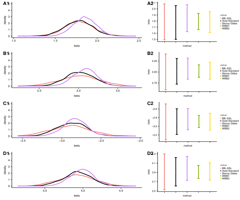
(a) Active predictors, from top to bottom: $\beta_{1},\beta_{2},\beta_{3},\beta_{4}$

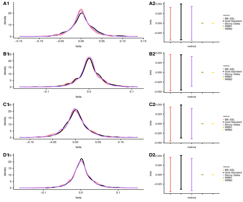
(b) Inactive predictors, from top to bottom: $\beta_{5},\beta_{6},\beta_{7},\beta_{8}$

Figure 6: Estimated posterior density (left panel) and $90\%$ credible intervals (right panel) of $\beta_{i}$’s when all covariatess are correlated with $\rho=0.6$. We have $n=100,p=1000,\beta_{active}=(2,3,-3,4)^{\prime},\lambda_{0}=50,\lambda_{1}=0.05$. BB-SSL is fitted using a single $\lambda_{0}$ and initialized at SSLASSO solution on the original $\boldsymbol{X},\boldsymbol{y}$. Since WBB1 and WBB2 produce a point mass at zero, we exclude them from density comparisons.

Setting	Block-wise $\rho=0.9$, $\beta_{active}=(1,2,-2,3)^{\prime}$									Block-wise $\rho=0.99$, $\beta_{active}=(2,4,-4,6)^{\prime}$
Metric	$\beta_{j}$’s						$\gamma_{j}$’s		Model	$\beta_{j}$’s						$\gamma_{j}$’s		Model
Metric	KL		JD of 90% CI		‘Bias’		‘Bias’		HD	KL		JD of 90% CI		‘Bias’		‘Bias’		HD
	$+$	$-$	$+$	$-$	$+$	$-$	$+$	$-$	all	$+$	$-$	$+$	$-$	$+$	$-$	$+$	$-$	all
Skinny Gibbs	0.19	0.009	0.30	0.10	0.04	0.003	*	*	0	2.00	0.02	0.62	0.10	0.68	0.005	0.15	0.002	2.2
WBB1	0.41	3.09	0.45	1	0.03	0.003	*	*	0	1.89	3.09	0.51	1	0.74	0.006	0.25	0.001	2
WBB2	0.21	3.09	0.37	1	0.03	0.003	*	*	0	1.89	3.09	0.52	1	0.74	0.006	0.25	0.001	2
BB-SSL	0.02	0.003	0.14	0.10	0.04	0.003	*	*	0	1.73	0.01	0.37	0.10	0.74	0.006	0.25	0.001	2
Setting	Equi-correlation $\rho=0.6$, $\beta_{active}=(2,3,-3,4)^{\prime}$									Equi-correlation $\rho=0.9$, $\beta_{active}=(2,3,-3,4)^{\prime}$
Metric	$\beta_{j}$’s						$\gamma_{j}$’s		Model	$\beta_{j}$’s						$\gamma_{j}$’s		Model
Metric	KL		JD of 90% CI		‘Bias’		‘Bias’		HD	KL		JD of 90% CI		‘Bias’		‘Bias’		HD
	$+$	$-$	$+$	$-$	$+$	$-$	$+$	$-$	all	$+$	$-$	$+$	$-$	$+$	$-$	$+$	$-$	all
Skinny Gibbs	0.13	0.01	0.23	0.11	0.05	0.003	0.0008	*	1	0.30	0.02	0.33	0.09	0.23	0.004	0.001	*	2
WBB1	0.12	3.09	0.30	1	0.03	0.003	*	*	0	0.14	3.08	0.23	1	0.13	0.002	*	*	0
WBB2	0.13	3.09	0.30	1	0.03	0.003	*	*	0	0.15	3.08	0.23	1	0.13	0.002	*	*	0
BB-SSL	0.06	0.003	0.20	$\boldsymbol{0.11}$	0.03	0.003	*	*	0	0.11	-0.003	0.23	0.08	0.12	0.002	*	*	0

Table 2: Evaluation of approximation properties (relative to SSVS) in the high-dimensional setting with $n=100$ and $p=1\,000$ based on 10 independent runs. The best performance is marked in bold font. KL is the Kullback-Leibler divergence, JD is the Jaccard distance of credible intervals (CI), HD is the Hamming distance of the median models. ‘Bias’ refers to the $l_{1}$ distance of estimated posterior means. We denote with $*$ all numbers smaller than 0.0001, with $+$ an average over active coordinates, and with $-$ an average over inactive coordinates.

To better quantify the performance of each method, we gauge the quality of the posterior approximation using various metrics in Table 2. The KL divergence is calculated using an R package “FNN” (Beygelzimer et al. (2013)), where all parameters are set to their default values. We also report the Jaccard distance of $90\%$ credible intervals relative to the SSVS benchmark. The Jaccard distance (Jaccard, 1912) of two intervals $A$ and $B$ is defined as $d_{J}(A,B)=1-J(A,B)$ where $J(A,B)=\frac{|A\cap B|}{|A\cup B|}$ and $|\cdot|$ denotes the length. The Hamming distance is calculated using an R package “e1071” (Meyer et al. (2014)). We also compare the $\ell_{1}$ norm of posterior means (i.e. “bias” relative to the SSVS standard) for $\beta_{i}$’s as well as $\gamma_{i}$’s. All methods do well in terms of MIP and the selected model (based on the median probability model rule). For $\beta_{i}$’s, all methods estimate the mean accurately. Taking into account the shape of the posterior for $\beta_{i}$’s, the performance is divided among coordinates and methods. For all methods, the approximability of active coordinates is less accurate than for the inactive ones. In the settings we tried, we rank the performance of various methods as follows: $\text{BB-SSL}\,>\,\text{Skinny Gibbs}\,>\,\text{WBB1}\,\approx\,\text{WBB2}$. The average times (in seconds (s) when $\rho=0.6$ in the equi-correlated design) spent on generating $100$ effective samples for each $\beta_{j}$ are: BB-SSL (0.69 s) $<$ SSVS2 (2.58 s) $<$ Skinny Gibbs (6.61 s) $<$ WBB2 (13.53 s) $<$ WBB1 (17.25 s) $<$ SSVS1 (34.67 s).

Conclusion

We found that BB-SSL is a reliable approximate method for posterior sampling that achieves a close-to-exact (SSVS) performance but is computationally cheaper. Additional speedups can be obtained with parallelization. The most expensive step in BB-SSL is solving the optimization problem (13) at each iteration. This could be potentially circumvented by using the Generative Bootstrap Sampler (GBS) (Shin et al., 2020) which constructs a generator function that can transform weights into samples from the posterior distribution. This strategy could be particularly beneficial when both $n$ and $p$ are large and when many posterior samples are needed. While MCMC-based methods are sensitive to the initialization and can fall into a local trap (e.g. when predictors are highly correlated), we have seen BB-SSL to be less susceptible to this problem. BB-SSL, in some sense, relies on the optimization procedure not finding the global mode at all times. Indeed, we want to provide a representation of the entire posterior distribution consisting of both local and global modes. However, we anticipate that the global mode will be found more often, correctly reflecting the amount of posterior mass assigned to it. This issue was also discussed in Section 2.5.1 in Fong et al. (2019), who point out that not necessarily finding the global mode will result in assigning more posterior density to local modes. We have found BB-SSL (initialized at the SS-LASSO solution after annealing) perform similarly as SSVS initialized at the truth in very highly correlated cases.

6 Data Analysis

6.1 Life Cycle Savings Data

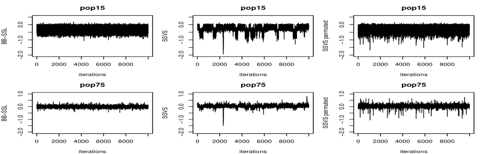
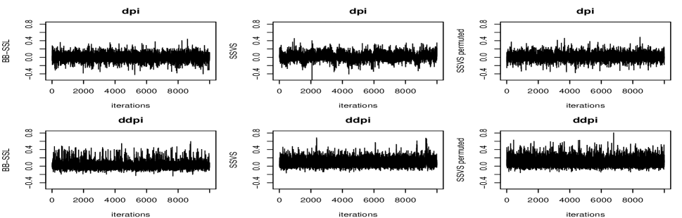
Figure 7: Trace plots for the Life Cycle Savings data. We choose $\lambda_{0}=20,\lambda_{1}=0.05$. The first column is the BB-SSL traceplot with weight distribution $\alpha=2\log\frac{(1-\theta)\lambda_{0}}{\theta\lambda_{1}}=14$, the second column is thinned SSVS traceplot chain with a LASSO initialization (regularization parameter chosen by cross validation). The third column is the same SSVS chain only with samples permuted.

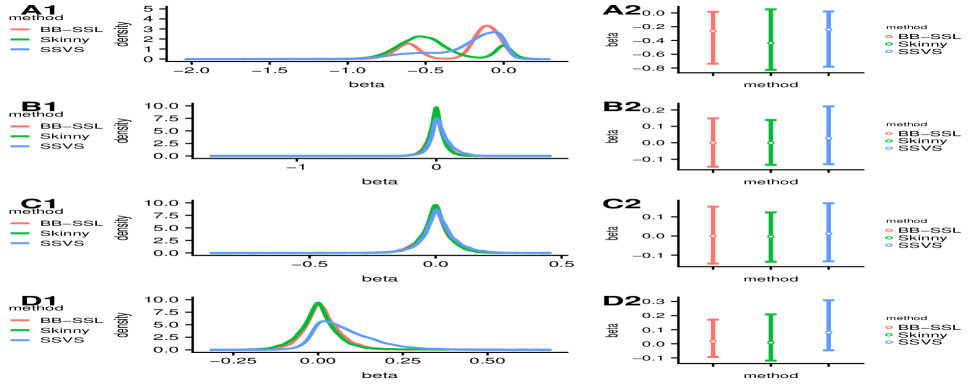
(a) Density of $\beta_{i}$’s..

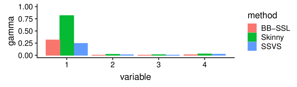
(b) Comparison of mean of $\gamma_{i}$’s.

Figure 8: Plots for Life Cycle Savings Data. We choose $\lambda_{0}=20,\lambda_{1}=0.05$. SSVS is initialized at the LASSO solution (with the regularization parameter chosen by cross-validation). The weight distribution for BB-SSL uses $\alpha=2\log\frac{(1-\theta)\lambda_{0}}{\theta\lambda_{1}}=14$.

The Life Cycle Savings data (Belsley et al., 2005) consists of $n=50$ observations on $p=4$ highly correlated predictors: “pop15” (percentage of population under 15 years old), “pop75” (percentage of population over 75 years old), “dpi” (per-capita disposable income), “ddpi” (percentage of growth rate of dpi). According to the life-cycle savings hypothesis proposed by Ando and Modigliani (1963), the savings ratio ($y$) can be explained by these four predictors and a linear model can be used to model their relationship.

We preprocess the data in the following way. First, we standardize predictors so that each column of $\boldsymbol{X}$ is centered and rescaled so that $||\boldsymbol{X}_{j}||_{2}=\sqrt{n}$. Next, we estimate the noise variance $\sigma^{2}$ using an ordinary least squares regression. We then divide $y$ by the estimated noise standard deviation and estimate $\theta$ by fitting SSL with $\lambda_{0}=20,\lambda_{1}=0.05$. For BB-SSL we set $\alpha=2\log\frac{(1-\theta)\lambda_{0}}{\theta\lambda_{1}}\approx 14$ and set $a=1$, $b=4$. We run SSVS1 and Skinny Gibbs for $T=100\,000,\,B=5\,000$ and BB-SSL for $T=10\,000$.

Figure 7 shows the trace plots on the four predictors. BB-SSL (first column) has the same mean and spread as SSVS (third column). We also observe that raw samples from SSVS (second column) are correlated, so more iterations are needed in order to fully explore the posterior. In contrast, each sample from BB-SSL is independent and thereby fewer samples will be needed in practice. See Table 3 for effective sample size comparisons. Figure 8(a) shows the marginal density of $\beta_{i}$’s and 8(b) shows the marginal mean of $\gamma_{i}$’s. In both figures BB-SSL achieves good performance.

	SSVS	Skinny Gibbs	BB-SSL
Effective sample size	2716	11188	15000

Table 3: Average effective sample size (out of $15\,000$ samples) for Life Cycle Saving Data. Effective sample size is calculated using R package coda (Plummer et al. (2006)).

6.2 Durable Goods Marketing Data Set

Our second application examines a cross-sectional dataset from Ni et al. (2012) (ISMS Durable Goods Dataset 2) consisting of durable goods sales data from a major anonymous U.S. consumer electronics retailer. The dataset features the results of a direct-mail promotion campaign in November 2003 where roughly half of the $n=176\,961$ households received a promotional mailer with $10\$$ off their purchase during the promotion time period (December 4-15). The treatment assignment ($tr_{i}=\mathbb{I}\left(\text{promotional mailer}_{i}\right)$) was random. The data contains $146$ descriptors of all customers including prior purchase history, purchase of warranties etc. We will investigate the effect of the promotional campaign (as well as other covariates) on December sales. In addition, we will interact the promotion mail indicator with customer characteristics to identify the “mail-deal-prone” customers. To be more specific, we adopt the following model

$$Y_{i}=\alpha\times tr_{i}+\boldsymbol{\beta}^{T}\boldsymbol{x}_{i}+\boldsymbol{\gamma}\times tr_{i}\times\boldsymbol{x}_{i}+\epsilon_{i}$$ (19)

where $\boldsymbol{x}_{i}$ refers to the 146 covariates, $tr_{i}$ is the treatment assignment, and the noise $\epsilon_{i}$ is iid normally distributed. And our aim is to (1) estimate the coefficients $\alpha,\boldsymbol{\beta},\boldsymbol{\gamma}$; (2) identify those customers with $\mathbb{E}\left[Y_{i}\,|\>\boldsymbol{x}_{i},tr_{i}=1\right]>\mathbb{E}\left[Y_{i}\,|\>\boldsymbol{x}_{i},tr_{i}=0\right]$.

For preprocessing, we first remove all variables that contain missing values or that are all $0$’s. We also create new predictors by interacting the treatment effect with the descriptor variables. After that the total number of predictors becomes $p=273$. We standardize $\boldsymbol{X}$ such that each column has a zero mean and a standard deviation $\sqrt{n}$ and we use the maximum likelihood estimate of the standard deviation to rescale the outcome. We run BB-SSL for $T=1\,000$ iterations and SSVS1 for $T=20\,000$ iterations with a $B=1\,000$ burnin period, initializing MCMC at the origin. We set $\lambda_{0}=100,\lambda_{1}=0.05,a=1,b=p$. Estimating $\hat{\theta}=\frac{\text{\# of selected variables}}{p}$ by fitting the Spike-and-Slab LASSO, we then set $\alpha=2\log\frac{(1-\hat{\theta})\theta_{0}}{\hat{\theta}\lambda_{1}}$.

Figure 10 depicts estimated posterior density of selected coefficients in the model (19), showing that BB-SSL estimation is very close to the gold standard (SSVS). Further, BB-SSL identified $67.3\%$ of customers as “mail-deal-prone”, reaching accuracy $98.2\%$ and a false positive rate $2.1\%$ (treating SSVS estimation as the truth). Despite the comparable performance to SSVS, BB-SSL is advantageous in terms of computational efficiency. As shown in Figure 9, within the same amount of time, BB-SSL obtains more effective samples compared with SSVS and its advantage becomes even more significant as time increases. This experiment confirms our hypothesis that BB-SSL has a great potential as an approximate method for large datasets.

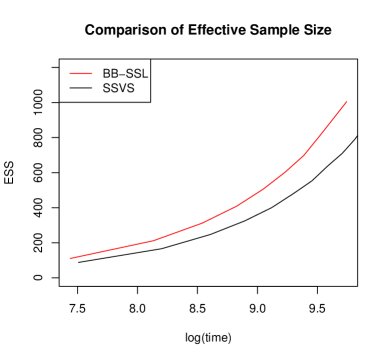
Figure 9: Effective sample size comparison for ISMS Durable Goods Dataset 2. We choose $\lambda_{0}=100,\lambda_{1}=0.05$. Red line is BB-SSL with $\alpha=2\log\frac{(1-\theta)\lambda_{0}}{\theta\lambda_{1}}\approx 15$ and black line is SSVS initialized at origin.

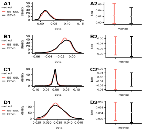
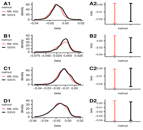
Figure 10: Posterior density and credible intervals for the selected $\beta_{i}$’s. From left to right, top to bottom they correspond to “S-SAL-TOT60M”, “S-U-CLS-NBR-12MO”, “PH-HOLIDAY-MAILER-RESP-SA”, “PROMO-NOV-SALES”, “S-SAL-FALL-24MO”, “S-TOT-CAT $\times$ treatment”, “C-ESP-RECT $\times$ treatment”, “S-CNT-TOT24M $\times$ treatment”. We set $\lambda_{0}=100,\lambda_{1}=0.05,a=1,b=273$. We set $\alpha=2\log\frac{(1-\theta)\lambda_{0}}{\theta\lambda_{1}}\approx 15$.

7 Discussion

In this paper we developed BB-SSL, a computational approach for approximate posterior sampling under Spike-and-Slab LASSO priors based on Bayesian bootstrap ideas. The fundamental premise of BB-SSL is the following: replace sampling from conditionals (which can be costly when either $n$ or $p$ are large) with fast optimization of randomly perturbed (reweigthed) posterior densities. We have explored various ways of performing the perturbation and looked into asymptotics for guidance about perturbing (weighting) distributions. We have concluded that with suitable conditions on the weights distribution, the pseudo-posterior distribution attains the same rate as the actual posterior in high-dimensional estimation problems (sparse normal means and high-dimensional regression). These theoretical results are reassuring and significantly extend existing knowledge about Weighted Likelihood Bootstrap (Newton et al. (2020)), which was shown to be consistent for iid data in finite-dimensional problems. We have shown in simulations and on real data that BB-SSL can approximate the true posterior well and can be computationally beneficial. The GBS method of Shin et al. (2020) could potentially greatly improve the scalability of BB-SSL. We leave this direction for future research.

Appendix A Proofs

This section presents proofs of the main theoretical statements: Section A.1 shows the proof of Theorem 4.1. Section A.2 presents the proof of Corollary 4.1. Section A.3 shows an example for the remark under Theorem 4.1. Section A.4 proves Theorem 4.2 and Theorem 4.3. Section A.5 proves Corollary 4.1. Section A.6 introduces a motivation for Section 3.1.

A.1 Proof of Theorem 4.1

A.1.1 Definitions and Lemmas used in the proof of Theorem 4.1

Denote constants

$$c_{+}^{\lambda_{0},\lambda_{1}}=0.5(1+\sqrt{1-4/(\lambda_{0}-\lambda_{1})^{2}})$$

and

$$\delta_{c+}^{\lambda_{0},\lambda_{1}}=\frac{1}{\lambda_{0}-\lambda_{1}}\log\left[\frac{1-\theta}{\theta}\frac{\lambda_{0}}{\lambda_{1}}\frac{c_{+}}{1-c_{+}}\right].$$

With slight abuse of notation, we denote the marginal prior (after integrating out $\gamma_{i}$) by

$$\pi(\beta_{i}\mid\theta,\lambda_{0},\lambda_{1})=\theta\lambda_{1}/2e^{-|\beta_{i}|\lambda_{1}}+(1-\theta)\lambda_{0}/2e^{-|\beta_{i}|\lambda_{0}}.$$

Similarly as in Ročková (2018a), the conditional mixing weight between the spike and the slab will be denoted with

$$p^{*}(t;\lambda_{0},\lambda_{1})=\frac{\theta\lambda_{1}e^{-|t|\lambda_{1}}}{\theta\lambda_{1}e^{-|t|\lambda_{1}}+(1-\theta)\lambda_{0}e^{-|t|\lambda_{0}}}$$ (20)

and the weighted penalty with

$$\lambda^{*}(t;\lambda_{0},\lambda_{1})=\lambda_{1}p^{*}(t;\lambda_{0},\lambda_{1})+\lambda_{0}(1-p^{*}(t;\lambda_{0},\lambda_{1})).$$

The quantities $p^{*}(t;\lambda_{0},\lambda_{1})$ and $\lambda^{*}(t;\lambda_{0},\lambda_{1})$ are analogues of $p^{\star}_{\theta}$ and $\lambda^{\star}_{\theta}$ defined in (5) (main manuscript). Here, we have emphasized the dependence on $\lambda_{1}$ and $\lambda_{0}$ and suppressed the dependence on $\theta$ since this parameter is treated as fixed in our theory. Finally, we denote

$$\rho(t\,|\>\theta,\lambda_{0},\lambda_{1})=-\lambda_{1}|t|+\log[p^{*}(0;\lambda_{0},\lambda_{1})/p^{*}(t;\lambda_{0},\lambda_{1})]$$

and (similarly as in Ročková (2018a))

$$g(t;\lambda_{0},\lambda_{1})=[\lambda^{*}(t;\lambda_{0},\lambda_{1})-\lambda_{1}]^{2}+2\log p^{*}(t;\lambda_{0},\lambda_{1}).$$

The following Lemma (a version of Theorem 3.1 in Ročková (2018a)) will be useful for characterizing the BB-SSL posterior properties.

Lemma A.1.

Assume $Y_{i}$’s arise from the normal means model (14) with $\sigma=1$ for $1\leq i\leq n$. Under the SSL prior (2), the mode $\smash{\widehat{\boldsymbol{\beta}}}=(\smash{\widehat{\beta}}_{1},\cdots,\smash{\widehat{\beta}}_{p})^{T}$ maximizing $L(\boldsymbol{\beta},\boldsymbol{Y})=-\frac{1}{2}\sum_{i=1}^{n}(Y_{i}-\beta_{i})^{2}+\sum_{i=1}^{n}\rho(\beta_{i}\,|\>\theta,\lambda_{0},\lambda_{1})$ satisfies

$$\smash{\widehat{\beta}}_{i}=\begin{cases}0,&\text{if $|Y_{i}|\leq\Delta(\lambda_{0},\lambda_{1})$}.\\ {}[|Y_{i}|-\lambda^{*}(\smash{\widehat{\beta_{i}}};\lambda_{0},\lambda_{1})]_{+}\text{sign}(Y_{i}),&\text{otherwise}.\end{cases}$$ (21)

where

$$\Delta(\lambda_{0},\lambda_{1})=\inf_{t>0}[t/2-\rho(t\mid\theta,\lambda_{0},\lambda_{1})/t].$$

Notice that $\Delta(\lambda_{0},\lambda_{1})$ is the normal-means analogue of $\Delta_{j}$ (defined below (4) in the main manuscript) where we have added $(\lambda_{0},\lambda_{1})$ to emphasize its dependence on $\lambda_{0}$ and $\lambda_{1}$. Next, we will need an upper and lower bound for $\Delta(\lambda_{0},\lambda_{1})$. When $\lambda_{0}-\lambda_{1}>2$ and $g(0;\lambda_{0},\lambda_{1})>0$, $-\frac{1}{2}(Y_{i}-\beta)^{2}+\rho(\beta\,|\>\theta,\lambda_{0},\lambda_{1})$ has two modes and Ročková (2018a) shows that $\Delta(\lambda_{0},\lambda_{1})$ can also be written as

$$\Delta(\lambda_{0},\lambda_{1})=\sqrt{2\log[1/p^{*}(0;\lambda_{0},\lambda_{1})]+g(\widetilde{\beta};\lambda_{0},\lambda_{1})}+\lambda_{1},$$

where $\widetilde{\beta}$ is the local mode (not the global mode) of $-\frac{1}{2}(Y_{i}-\beta)^{2}+\rho(\beta\,|\>\theta,\lambda_{0},\lambda_{1})$. It follows from Theorem 3.1 in Ročková (2018a) and Lemma 1.2 in the Appendix of Ročková (2018a) that

$$\Delta^{L}(\lambda_{0},\lambda_{1})<\Delta(\lambda_{0},\lambda_{1})\leq\Delta^{U}(\lambda_{0},\lambda_{1}),$$ (22)

where

$$\Delta^{L}(\lambda_{0},\lambda_{1})=\sqrt{2\log[1/p^{*}(0;\lambda_{0},\lambda_{1})]-2}+\lambda_{1}\quad\text{and}\quad\Delta^{U}(\lambda_{0},\lambda_{1})=\sqrt{2\log[1/p^{*}(0;\lambda_{0},\lambda_{1})]}+\lambda_{1}.$$

Based on these facts, we then obtain the following simple Lemma.

Lemma A.2.

Under assumptions in Theorem 4.1, for any $w_{i}>0$ which satisfies

$$g(0;\lambda_{0}w_{i}^{-1/2},\lambda_{1}w_{i}^{-1/2})>0\quad\text{and}\quad\lambda_{0}w_{i}^{-1/2}-\lambda_{1}w_{i}^{-1/2}>2$$

we have

$$\Delta^{L}(\lambda_{0},\lambda_{1})+\lambda_{1}(w_{i}^{-1/2}-1)\leq\Delta(\lambda_{0}w_{i}^{-1/2},\lambda_{1}w_{i}^{-1/2})\leq\Delta^{U}(\lambda_{0},\lambda_{1})+\lambda_{1}(w_{i}^{-1/2}-1).$$ (23)

Proof.

Since $g(0;\lambda_{0}w_{i}^{-1/2},\lambda_{1}w_{i}^{-1/2})>0$ and $\lambda_{0}w_{i}^{-1/2}-\lambda_{1}w_{i}^{-1/2}>2$, from Lemma A.1 (the discussion below) and the fact that $p^{*}(0;\lambda_{0},\lambda_{1})=p^{*}(0;\lambda_{0}w_{i}^{-1/2},\lambda_{1}w_{i}^{-1/2})$, we have

$$\Delta(\lambda_{0}w_{i}^{-1/2},\lambda_{1}w_{i}^{-1/2})\leq\Delta^{U}(\lambda_{0}w_{i}^{-1/2},\lambda_{1}w_{i}^{-1/2})=\Delta^{U}(\lambda_{0},\lambda_{1})+\lambda_{1}(w_{i}^{-1/2}-1).$$

The other inequality is obtained similarly.∎

Lemma A.3.

For any fixed constant $C>0$, $\mu\in\mathbb{R}$ and a random variable $Y\sim N(0,1)$, we have

$$\mathbb{E}_{Y}\left[|Y-\mu|^{2}\mathbb{I}(|Y-\mu|\geq C)\right]$$

$$\quad=1+\mu^{2}-\Phi(\mu+C)+\Phi(\mu-C)-(\mu-C)\phi(\mu-C)+(\mu+C)\phi(\mu+C),$$

where $\Phi$ and $\phi$ are the standard normal distribution and density functions.

Proof.

Denote a truncated normal random variable with $Z=[Y\mid Y\in[a,b]]$ and recall that

$$\mathbb{E}\left[Z\right]=\frac{\phi(a)-\phi(b)}{\Phi(b)-\Phi(a)}\quad\text{and}\quad\mathbb{E}\left[Z^{2}\right]=1+\frac{a\phi(a)-b\phi(b)}{\Phi(b)-\Phi(a)}.$$

Then we have

$$\mathbb{E}_{Y}\left[|Y-\mu|^{2}\mathbb{I}(|Y-\mu|\geq C)\right]$$

$$=\mathbb{E}_{Y}\left[|Y-\mu|^{2}\right]-\mathbb{E}_{Y}\left[|Y-\mu|^{2}\mathbb{I}(|Y-\mu|<C)\right]$$

$$=1+\mu^{2}-\left[\Phi(\mu+C)-\Phi(\mu-C)\right]$$

$$\quad\times\left[\mathbb{E}\left[Y^{2}\mid Y\in[\mu-C,\mu+C]\right]-2\mu\mathbb{E}\left[Y\mid Y\in[\mu-C,\mu+C]\right]+\mu^{2}\right]$$

$$=1+\mu^{2}-\Phi(\mu+C)+\Phi(\mu-C)-(\mu-C)\phi(\mu-C)+(\mu+C)\phi(\mu+C).\qed$$

A.1.2 Proof of Theorem 4.1

First assume that $\sigma=1$. Throughout this section, we will simply denote $\boldsymbol{Y}=\boldsymbol{Y}^{(n)}$. We want to obtain the expression for BB-SSL estimate $\widetilde{\boldsymbol{\beta}}$. Notice that the objective function (13) for BB-SSL can be written as

$$\begin{split}\widetilde{\boldsymbol{\beta}}&=\arg\max_{\boldsymbol{\beta}\in\mathbb{R}^{p}}\left\{-\sum_{i=1}^{n}\frac{w_{i}}{2}(Y_{i}-\beta_{i})^{2}+\sum_{i=1}^{n}\log\pi(\beta_{i}-\mu_{i}\,|\>\theta)\right\}\\ &=\arg\max_{\boldsymbol{\beta}\in\mathbb{R}^{p}}\left\{-\sum_{i=1}^{n}\frac{1}{2}(Y_{i}^{*}-\beta_{i}^{*})^{2}+\sum_{i=1}^{n}\log\pi_{i}^{*}(\beta_{i}^{*}\,|\>\theta)\right\},\end{split}$$ (24)

where $Y_{i}^{*}=w_{i}^{1/2}(Y_{i}-\mu_{i})$, $\beta_{i}^{*}=w_{i}^{1/2}(\beta_{i}-\mu_{i})$, and $\pi_{i}^{*}(\beta_{i}^{*}\,|\>\theta)=\pi(\beta_{i}^{*}\,|\>\theta,\lambda_{0}w_{i}^{-1/2},\lambda_{1}w_{i}^{-1/2})$. So from (21), the mode estimator $\smash{\widehat{\beta_{i}^{*}}}$ for $\beta_{i}^{*}$ satisfies

$$\smash{\widehat{\beta_{i}^{*}}}=\begin{cases}0,&\text{if $|Y_{i}^{*}|\leq\Delta(\lambda_{0}w_{i}^{-1/2},\lambda_{1}w_{i}^{-1/2})$}.\\ {}[|Y_{i}^{*}|-\lambda^{*}(\smash{\widehat{\beta_{i}^{*}}};\lambda_{0}w_{i}^{-1/2},\lambda_{1}w_{i}^{-1/2})]_{+}\text{sign}(Y_{i}^{*}),&\text{otherwise}.\end{cases}$$

The BB-SSL estimate $\boldsymbol{\widetilde{\boldsymbol{\beta}}}=(\widetilde{\beta}_{1},\cdots,\widetilde{\beta}_{p})^{T}$ can then be calculated via $\widetilde{\beta}_{i}=\smash{\widehat{\beta_{i}^{*}}}w_{i}^{-1/2}+\mu_{i}$. Equation (3.2) in Ročková (2018a) says that

$$\lambda^{*}(\beta_{i};\lambda_{0},\lambda_{1})=-\frac{\partial\rho(\beta_{i}\,|\>\theta,\lambda_{0},\lambda_{1})}{\partial|\beta_{i}|}.$$

From the chain rule and the fact that

$$\rho\left(w_{i}^{1/2}(\widetilde{\beta_{i}}-\mu_{i});\lambda_{0}w_{i}^{-1/2},\lambda_{1}w_{i}^{-1/2}\right)=\rho(\widetilde{\beta_{i}}-\mu_{i};\lambda_{0},\lambda_{1}),$$

we know

$$\lambda^{*}(\widehat{\beta_{i}^{*}};\lambda_{0}w_{i}^{-1/2},\lambda_{1}w_{i}^{-1/2})=\lambda^{*}\left(w_{i}^{1/2}\left(\widetilde{\beta_{i}}-\mu_{i}\right);\lambda_{0}w_{i}^{-1/2},\lambda_{1}w_{i}^{-1/2}\right)$$

$$=-\frac{\partial\rho\left(w_{i}^{1/2}(\widetilde{\beta_{i}}-\mu_{i});\lambda_{0}w_{i}^{-1/2},\lambda_{1}w_{i}^{-1/2}\right)}{\partial\left|w_{i}^{1/2}(\widetilde{\beta_{i}}-\mu_{i})\right|}$$

$$=-\frac{\partial\rho(\widetilde{\beta_{i}}-\mu_{i};\lambda_{0},\lambda_{1})}{\partial\left|\widetilde{\beta_{i}}-\mu_{i}\right|}\frac{\partial\left|\widetilde{\beta_{i}}-\mu_{i}\right|}{\partial\left|w_{i}^{1/2}\left(\widetilde{\beta_{i}}-\mu_{i}\right)\right|}=w_{i}^{-1/2}\lambda^{*}\left(\widetilde{\beta_{i}}-\mu_{i};\lambda_{0},\lambda_{1}\right).$$

Thus,

$$\widetilde{\beta}_{i}=\begin{cases}&\mu_{i},\quad\text{if $|w_{i}^{1/2}(Y_{i}-\mu_{i})|\leq\Delta(\lambda_{0}w_{i}^{-1/2},\lambda_{1}w_{i}^{-1/2})$}.\\ &\mu_{i}+[|Y_{i}-\mu_{i}|-w_{i}^{-1}\lambda^{*}(\widetilde{\beta}_{i}-\mu_{i};\lambda_{0},\lambda_{1})]_{+}\text{sign}(Y_{i}-\mu_{i}),\quad\text{otherwise}.\end{cases}$$ (25)

From the Markov’s inequality, we know that for any $M_{n}>0$,

$$\mathbb{E}_{\boldsymbol{Y}}\mathbb{P}_{\boldsymbol{\mu},\boldsymbol{w}}\left(\|\widetilde{\boldsymbol{\beta}}-\boldsymbol{\beta}^{0}\|_{2}^{2}>M_{n}q\log\left(\frac{n}{q}\right)\,|\>\boldsymbol{Y}\right)\leq\frac{\mathbb{E}_{\boldsymbol{Y}}\mathbb{E}_{\boldsymbol{\mu},\boldsymbol{w}}\left[\|\widetilde{\boldsymbol{\beta}}-\boldsymbol{\beta}^{0}\|_{2}^{2}\,|\>\boldsymbol{Y}\right]}{M_{n}q\log\frac{n}{q}}.$$

Thus, in order to prove the desired statement, we only need to bound $\mathbb{E}_{\boldsymbol{Y}}\left[\mathbb{E}_{\boldsymbol{\mu},\boldsymbol{w}}\left[\|\widetilde{\boldsymbol{\beta}}-\boldsymbol{\beta}^{0}\|_{2}^{2}\,|\>\boldsymbol{Y}\right]\right]$. Notice that for the separable SSL prior (i.e. with a fixed value of $\theta$), the posterior is separable and we obtain

$$\mathbb{E}_{\boldsymbol{Y}}\left[\mathbb{E}_{\boldsymbol{\mu},\boldsymbol{w}}\left[\|\widetilde{\boldsymbol{\beta}}-\boldsymbol{\beta}^{0}\|_{2}^{2}\,|\>\boldsymbol{Y}\right]\right]=\sum_{i=1}^{n}\mathbb{E}_{Y_{i}}\left[\mathbb{E}_{\mu_{i},w_{i}}\left[(\widetilde{\beta_{i}}-\beta_{i}^{0})^{2}\mid Y_{i}\right]\right].$$

We will bound the risk $\mathbb{E}_{Y_{i}}\left[\mathbb{E}_{\mu_{i},w_{i}}\left[(\widetilde{\beta_{i}}-\beta_{i}^{0})^{2}\mid Y_{i}\right]\right]$ separately for active and inactive coordinates.

Active coordinates

For active coordinates, we have

$$\begin{split}&\mathbb{E}_{Y_{i}}\left[\mathbb{E}_{\mu_{i},w_{i}}\left[(\widetilde{\beta_{i}}-\beta_{i}^{0})^{2}\mid Y_{i}\right]\right]=\mathbb{E}_{Y_{i}}\left[\mathbb{E}_{\mu_{i},w_{i}}\left[(\widetilde{\beta_{i}}-Y_{i}+Y_{i}-\beta_{i}^{0})^{2}\mid Y_{i}\right]\right]\\ \leq\,\,&\mathbb{E}_{Y_{i}}\left[2\mathbb{E}_{\mu_{i},w_{i}}\left[(\widetilde{\beta_{i}}-Y_{i})^{2}\mid Y_{i}\right]+2\mathbb{E}_{\mu_{i},w_{i}}\left[(Y_{i}-\beta_{i}^{0})^{2}\mid Y_{i}\right]\right]\\ \leq\,\,&2\mathbb{E}_{Y_{i}}\left[\mathbb{E}_{\mu_{i},w_{i}}\left[(\widetilde{\beta_{i}}-Y_{i})^{2}\mid Y_{i}\right]\right]+2\\ =\,\,&2\mathbb{E}_{Y_{i}}\left[\mathbb{E}_{\mu_{i},w_{i}}\left[(\widetilde{\beta_{i}}-Y_{i})^{2}\mathbb{I}\left(w_{i}^{1/2}|Y_{i}-\mu_{i}|\leq\Delta(\lambda_{0}w_{i}^{-1/2},\lambda_{1}w_{i}^{-1/2})\right)\mid Y_{i}\right]\right]\\ \,\,&+2\mathbb{E}_{Y_{i}}\left[\mathbb{E}_{\mu_{i},w_{i}}\left[(\widetilde{\beta_{i}}-Y_{i})^{2}\mathbb{I}\left(w_{i}^{1/2}|Y_{i}-\mu_{i}|>\Delta(\lambda_{0}w_{i}^{-1/2},\lambda_{1}w_{i}^{-1/2})\right)\mid Y_{i}\right]\right]+2\\ =\,\,&2U_{1}+2U_{2}+2,\end{split}$$ (26)

where

$$U_{1}=\mathbb{E}_{Y_{i}}\left[\mathbb{E}_{\mu_{i},w_{i}}\left[(\widetilde{\beta_{i}}-Y_{i})^{2}\mathbb{I}\left(w_{i}^{1/2}|Y_{i}-\mu_{i}|\leq\Delta(\lambda_{0}w_{i}^{-1/2},\lambda_{1}w_{i}^{-1/2})\right)\mid Y_{i}\right]\right],$$

$$U_{2}=\mathbb{E}_{Y_{i}}\left[\mathbb{E}_{\mu_{i},w_{i}}\left[(\widetilde{\beta_{i}}-Y_{i})^{2}\mathbb{I}\left(w_{i}^{1/2}|Y_{i}-\mu_{i}|>\Delta(\lambda_{0}w_{i}^{-1/2},\lambda_{1}w_{i}^{-1/2})\right)\mid Y_{i}\right]\right].$$

Now we bound $U_{1}$ and $U_{2}$ separately. First,

$$\begin{split}U_{1}&=\mathbb{E}_{Y_{i}}\left[\mathbb{E}_{\mu_{i},w_{i}}\left[(\widetilde{\beta_{i}}-Y_{i})^{2}\mathbb{I}\left(w_{i}^{1/2}|Y_{i}-\mu_{i}|\leq\Delta(\lambda_{0}w_{i}^{-1/2},\lambda_{1}w_{i}^{-1/2})\right)\mid Y_{i}\right]\right]\\ &\stackrel{{\scriptstyle(a)}}{{\leq}}\mathbb{E}_{Y_{i}}\left[\mathbb{E}_{\mu_{i},w_{i}}\left[(\mu_{i}-Y_{i})^{2}\mathbb{I}\left(|Y_{i}-\mu_{i}|\leq w_{i}^{-1/2}\Delta(\lambda_{0}w_{i}^{-1/2},\lambda_{1}w_{i}^{-1/2})\right)\mid Y_{i}\right]\right]\\ &\leq\mathbb{E}_{w_{i}}\left[\Delta^{2}(\lambda_{0}w_{i}^{-1/2},\lambda_{1}w_{i}^{-1/2})\frac{1}{w_{i}}\right],\end{split}$$ (27)

where $(a)$ utilizes the observation $|\widetilde{\beta_{i}}-Y_{i}|\leq|\mu_{i}-Y_{i}|$ from Equation (25). Deploying Lemma A.2 in equation (27), we get (when $n$ is sufficiently large)

$$\begin{split}U_{1}&\leq\mathbb{E}_{w_{i}}\left[\Delta^{2}(\lambda_{0}w_{i}^{-1/2},\lambda_{1}w_{i}^{-1/2})\frac{1}{w_{i}}\mathbb{I}\left(g(0;\lambda_{0}w_{i}^{-1/2},\lambda_{1}w_{i}^{-1/2})>0\,\,\text{and}\,\,\lambda_{0}w_{i}^{-1/2}-\lambda_{1}w_{i}^{-1/2}>2\right)\right]\\ &\quad+\mathbb{E}_{w_{i}}\left[\Delta^{2}(\lambda_{0}w_{i}^{-1/2},\lambda_{1}w_{i}^{-1/2})\frac{1}{w_{i}}\mathbb{I}\left(g(0;\lambda_{0}w_{i}^{-1/2},\lambda_{1}w_{i}^{-1/2})\leq 0\,\,\text{or}\,\,\lambda_{0}w_{i}^{-1/2}-\lambda_{1}w_{i}^{-1/2}\leq 2\right)\right]\\ &\leq\mathbb{E}_{w_{i}}\left[\frac{1}{w_{i}}\left(\Delta^{U}(\lambda_{0},\lambda_{1})+\lambda_{1}w_{i}^{-1/2}-\lambda_{1}\right)^{2}\right]\\ &\quad+\mathbb{E}_{w_{i}}\left[\Delta^{2}(\lambda_{0}w_{i}^{-1/2},\lambda_{1}w_{i}^{-1/2})\frac{1}{w_{i}}\mathbb{I}\left(w_{i}\geq\frac{(\lambda_{0}-\lambda_{1})^{2}(1-p^{*}(0;\lambda_{0},\lambda_{1}))^{2}}{2\log(1/p^{*}(0;\lambda_{0},\lambda_{1}))}\,\,\text{or}\,\,w_{i}\geq\frac{(\lambda_{0}-\lambda_{1})^{2}}{4}\right)\right]\\ &\stackrel{{\scriptstyle(a)}}{{\leq}}2\left(\Delta^{U}(\lambda_{0},\lambda_{1})-\lambda_{1}\right)^{2}\mathbb{E}_{w_{i}}\frac{1}{w_{i}}+2\lambda_{1}^{2}\mathbb{E}_{w_{i}}\frac{1}{w_{i}^{2}}+\mathbb{E}_{w_{i}}\left[\frac{\lambda_{0}^{2}}{w_{i}}\frac{1}{w_{i}}\mathbb{I}\left(w_{i}\geq C(\lambda_{0},\lambda_{1})\right)\right]\\ &\leq 2\left(\Delta^{U}(\lambda_{0},\lambda_{1})-\lambda_{1}\right)^{2}\mathbb{E}_{w_{i}}\frac{1}{w_{i}}+2\mathbb{E}_{w_{i}}\frac{1}{w_{i}^{2}}+\frac{\lambda_{0}^{2}}{C^{2}(\lambda_{0},\lambda_{1})}\mathbb{P}\left(w_{i}\geq C(\lambda_{0},\lambda_{1})\right)\\ &\stackrel{{\scriptstyle(b)}}{{\leq}}2\left(\Delta^{U}(\lambda_{0},\lambda_{1})-\lambda_{1}\right)^{2}\mathbb{E}_{w_{i}}\frac{1}{w_{i}}+2\mathbb{E}_{w_{i}}\frac{1}{w_{i}^{2}}+\frac{\lambda_{0}^{2}}{C^{3}(\lambda_{0},\lambda_{1})}\\ &\leq 2\left(\Delta^{U}(\lambda_{0},\lambda_{1})-\lambda_{1}\right)^{2}\mathbb{E}_{w_{i}}\frac{1}{w_{i}}+2\mathbb{E}_{w_{i}}\frac{1}{w_{i}^{2}}+1,\end{split}$$ (28)

where $(a)$ uses the fact that $(a+b)^{2}\leq 2a^{2}+2b^{2}$, $\Delta(\lambda_{0}w_{i}^{-1/2},\lambda_{1}w_{i}^{-1/2})\leq\lambda_{0}w_{i}^{-1/2}$, and we denote $C(\lambda_{0},\lambda_{1})=\min\left\{\frac{(\lambda_{0}-\lambda_{1})^{2}(1-p^{*}(0;\lambda_{0},\lambda_{1}))^{2}}{2\log(1/p^{*}(0;\lambda_{0},\lambda_{1}))},\frac{(\lambda_{0}-\lambda_{1})^{2}}{4}\right\}$, and $(b)$ follows from the Markov’s inequality.

For $U_{2}$, we have

$$\begin{split}U_{2}=&\mathbb{E}_{Y_{i}}\left[\mathbb{E}_{\mu_{i},w_{i}}\left[(\widetilde{\beta_{i}}-Y_{i})^{2}\mathbb{I}\left(w_{i}^{1/2}(Y_{i}-\mu_{i})>\Delta(\lambda_{0}w_{i}^{-1/2},\lambda_{1}w_{i}^{-1/2})\right)\mid Y_{i}\right]\right]\\ \text{$$}\stackrel{{\scriptstyle(a)}}{{\leq}}&\mathbb{E}_{Y_{i}}\left[\mathbb{E}_{\mu_{i},w_{i}}\left[\left(w_{i}^{-1}\lambda^{*}(\widetilde{\beta_{i}}-\mu_{i})\right)^{2}\mathbb{I}\left(w_{i}^{1/2}|Y_{i}-\mu_{i}|>\Delta(\lambda_{0}w_{i}^{-1/2},\lambda_{1}w_{i}^{-1/2})\right)\mid Y_{i}\right]\right]\\ \leq&\mathbb{E}_{Y_{i}}\left[\mathbb{E}_{\mu_{i},w_{i}}\left[\left(w_{i}^{-1}\lambda^{*}(\widetilde{\beta_{i}}-\mu_{i})\right)^{2}\mathbb{I}\left(w_{i}^{1/2}|Y_{i}-\mu_{i}|>\Delta(\lambda_{0}w_{i}^{-1/2},\lambda_{1}w_{i}^{-1/2})\right)\right.\right.\\ &\quad\quad\left.\left.\mathbb{I}\left(\lambda_{0}w_{i}^{-1/2}-\lambda_{1}w_{i}^{-1/2}>2\,\,\text{and}\,\,g(0;\lambda_{0}w_{i}^{-1/2},\lambda_{1}w_{i}^{-1/2})>0\right)\mid Y_{i}\right]\right]\\ &+\mathbb{E}_{Y_{i}}\left[\mathbb{E}_{\mu_{i},w_{i}}\left[\left(w_{i}^{-1}\lambda^{*}(\widetilde{\beta_{i}}-\mu_{i})\right)^{2}\mathbb{I}\left(w_{i}^{1/2}|Y_{i}-\mu_{i}|>\Delta(\lambda_{0}w_{i}^{-1/2},\lambda_{1}w_{i}^{-1/2})\right)\right.\right.\\ &\quad\quad\quad\left.\left.\mathbb{I}\left(\lambda_{0}w_{i}^{-1/2}-\lambda_{1}w_{i}^{-1/2}\leq 2\right)\mid Y_{i}\right]\right]\\ &+\mathbb{E}_{Y_{i}}\left[\mathbb{E}_{\mu_{i},w_{i}}\left[\left(w_{i}^{-1}\lambda^{*}(\widetilde{\beta_{i}}-\mu_{i})\right)^{2}\mathbb{I}\left(w_{i}^{1/2}|Y_{i}-\mu_{i}|>\Delta(\lambda_{0}w_{i}^{-1/2},\lambda_{1}w_{i}^{-1/2})\right)\right.\right.\\ &\quad\quad\quad\left.\left.\mathbb{I}\left(g(0;\lambda_{0}w_{i}^{-1/2},\lambda_{1}w_{i}^{-1/2})\leq 0\right)\mid Y_{i}\right]\right]\\ =&U_{3}+U_{4}+U_{5},\end{split}$$ (29)

where $(a)$ utilizes the fact that $|\widetilde{\beta_{i}}-Y_{i}|\leq w_{i}^{-1}\lambda^{*}(\widetilde{\beta_{i}}-\mu_{i})$ from Equation (25), and we abbreviate $\lambda^{*}(\widetilde{\beta_{i}}-\mu_{i})=\lambda^{*}(\widetilde{\beta_{i}}-\mu_{i};\lambda_{0},\lambda_{1})$. In order to bound (29), we bound $U_{3},U_{4},U_{5}$ separately.

• To bound $U_{3}$: When $\lambda_{0}w_{i}^{-1/2}-\lambda_{1}w_{i}^{-1/2}>2$ and $g(0;\lambda_{0}w_{i}^{-1/2},\lambda_{1}w_{i}^{-1/2})>0$, following the proof of Theorem 4.1 in Ročková (2018a), we know that $|\widehat{\beta_{i}^{*}}|>\delta_{c+}^{\lambda_{0}/\sqrt{w_{i}},\lambda_{1}/\sqrt{w_{i}}}$ and thus $p^{*}(\widehat{\beta_{i}^{*}};\lambda_{0}w_{i}^{-1/2},\lambda_{1}w_{i}^{-1/2})>c_{+}^{\lambda_{0}/\sqrt{w_{i}},\lambda_{1}/\sqrt{w_{i}}}$. This implies $p^{*}(\widetilde{\beta_{i}}-\mu_{i};\lambda_{0},\lambda_{1})>c_{+}^{\lambda_{0}/\sqrt{w_{i}},\lambda_{1}/\sqrt{w_{i}}}$, so we have

  $$\lambda^{*}(\widetilde{\beta_{i}}-\mu_{i};\lambda_{0}w_{i}^{-1/2},\lambda_{1}w_{i}^{-1/2})<c_{+}^{\lambda_{0}/\sqrt{w_{i}},\lambda_{1}/\sqrt{w_{i}}}(\lambda_{1}w_{i}^{-1/2}-\lambda_{0}w_{i}^{-1/2})+\lambda_{0}w_{i}^{-1/2}$$

  $$= (1-c_{+}^{\lambda_{0}/\sqrt{w_{i}},\lambda_{1}/\sqrt{w_{i}}})(\lambda_{0}w_{i}^{-1/2}-\lambda_{1}w_{i}^{-1/2})+\lambda_{1}w_{i}^{-1/2}\stackrel{{\scriptstyle(a)}}{{<}}\frac{2w_{i}^{1/2}}{\lambda_{0}-\lambda_{1}}+\lambda_{1}w_{i}^{-1/2}<1+\lambda_{1}w_{i}^{-1/2},$$

  where $(a)$ follows from the fact that

  $$c_{+}^{\lambda_{0}/\sqrt{w_{i}},\lambda_{1}/\sqrt{w_{i}}}(1-c_{+}^{\lambda_{0}/\sqrt{w_{i}},\lambda_{1}/\sqrt{w_{i}}})=\frac{1}{(\lambda_{0}w_{i}^{-1/2}-\lambda_{1}w_{i}^{-1/2})^{2}}=\frac{w_{i}}{(\lambda_{0}-\lambda_{1})^{2}},$$

  and

  $$c_{+}^{\lambda_{0}/\sqrt{w_{i}},\lambda_{1}/\sqrt{w_{i}}}>0.5.$$

  In view that $\lambda^{*}(\widetilde{\beta_{i}}-\mu_{i};\lambda_{0}w_{i}^{-1/2},\lambda_{1}w_{i}^{-1/2})=w_{i}^{-1/2}\lambda^{*}(\widetilde{\beta_{i}}-\mu_{i};\lambda_{0},\lambda_{1})$, we have

  $$U_{3}\leq\mathbb{E}_{w_{i}}\left(\frac{w_{i}^{1/2}+\lambda_{1}}{w_{i}}\right)^{2}\leq 2\mathbb{E}_{w_{i}}\frac{1}{w_{i}}+2\lambda_{1}^{2}\mathbb{E}_{w_{i}}\frac{1}{w_{i}^{2}}.$$

• To bound $U_{4}$: When $\lambda_{0}w_{i}^{-1/2}-\lambda_{1}w_{i}^{-1/2}\leq 2$, we have

  $$\lambda^{*}(\widetilde{\beta_{i}}-\mu_{i};\lambda_{0}w_{i}^{-1/2},\lambda_{1}w_{i}^{-1/2})\leq\lambda_{0}w_{i}^{-1/2}\leq\lambda_{1}w_{i}^{-1/2}+2.$$

  So in view that $\lambda^{*}(\widetilde{\beta_{i}}-\mu_{i};\lambda_{0}w_{i}^{-1/2},\lambda_{1}w_{i}^{-1/2})=w_{i}^{-1/2}\lambda^{*}(\widetilde{\beta_{i}}-\mu_{i};\lambda_{0},\lambda_{1})$, we have

  $$U_{4}\leq\mathbb{E}_{w_{i}}\left(\frac{\lambda_{1}+2w_{i}^{1/2}}{w_{i}}\right)^{2}\leq 2\lambda_{1}^{2}\mathbb{E}_{w_{i}}\frac{1}{w_{i}^{2}}+8\mathbb{E}_{w_{i}}\frac{1}{w_{i}}.$$

• To bound $U_{5}$: When $g(0;\lambda_{0}w_{i}^{-1/2},\lambda_{1}w_{i}^{-1/2})\leq 0$, we have $w_{i}\geq\frac{(\lambda_{0}-\lambda_{1})^{2}(1-p^{*}(0;\lambda_{0},\lambda_{1}))^{2}}{2\log(1/p^{*}(0;\lambda_{0},\lambda_{1}))}$, thus when $n$ is sufficiently large,

  $$U_{5}\leq\mathbb{E}_{w_{i}}\left(\frac{\lambda_{0}}{w_{i}}\mathbb{I}\left(w_{i}\geq\frac{(\lambda_{0}-\lambda_{1})^{2}(1-p^{*}(0;\lambda_{0},\lambda_{1}))^{2}}{2\log(1/p^{*}(0;\lambda_{0},\lambda_{1}))}\right)\right)^{2}\leq\frac{4[\log(1/p^{*}(0;\lambda_{0},\lambda_{1}))]^{2}\lambda_{0}^{2}}{(\lambda_{0}-\lambda_{1})^{4}(1-p^{*}(0;\lambda_{0},\lambda_{1}))^{4}}\leq\frac{1}{\lambda_{0}}.$$

So plugging the above bounds into Equation (29), we obtain

$$U_{2}\leq U_{3}+U_{4}+U_{5}\leq 10\mathbb{E}_{w_{i}}\frac{1}{w_{i}^{2}}+4\lambda_{1}^{2}\mathbb{E}_{w_{i}}\frac{1}{w_{i}}+\frac{1}{\lambda_{0}}.$$ (30)

Thus, from (26), (28), (30) and condition (2), we know that for active coordinates, when $n$ is sufficiently large,

$$\mathbb{E}_{Y_{i}}\mathbb{E}_{\mu_{i},w_{i}}[(\widetilde{\beta}_{i}-\beta_{i}^{0})^{2}\,|\>Y]\leq 6+\left[4\left(\Delta^{U}(\lambda_{0},\lambda_{1})-\lambda_{1}\right)^{2}+8\lambda_{1}^{2}\right]\mathbb{E}_{w_{i}}\frac{1}{w_{i}}+24\mathbb{E}_{w_{i}}\frac{1}{w_{i}^{2}}$$

$$\leq C_{3}\left(\Delta^{U}(\lambda_{0},\lambda_{1})\right)^{2}.$$

Inactive coordinates

For inactive coordinates, we have

$$\begin{split}&\mathbb{E}_{Y_{i}}\left[\mathbb{E}_{\mu_{i},w_{i}}[(\widetilde{\beta_{i}}-\beta_{i}^{0})^{2}\,|\>Y_{i}]\right]=\mathbb{E}_{Y_{i}}\left[\mathbb{E}_{\mu_{i},w_{i}}[(\widetilde{\beta_{i}})^{2}\,|\>Y_{i}]\right]\\ =&\mathbb{E}_{Y_{i}}\left[\mathbb{E}_{\mu_{i},w_{i}}\left[(\widetilde{\beta_{i}}-\mu_{i}+\mu_{i})^{2}\mathbb{I}(\sqrt{w_{i}}|Y_{i}-\mu_{i}|\geq\Delta(\lambda_{0}w_{i}^{-1/2},\lambda_{1}w_{i}^{-1/2}))\,|\>Y_{i}\right]\right]\\ &+\mathbb{E}_{Y_{i}}\left[\mathbb{E}_{\mu_{i},w_{i}}\left[(\widetilde{\beta_{i}})^{2}\mathbb{I}(\sqrt{w_{i}}|Y_{i}-\mu_{i}|<\Delta(\lambda_{0}w_{i}^{-1/2},\lambda_{1}w_{i}^{-1/2}))\,|\>Y_{i}\right]\right]\\ \stackrel{{\scriptstyle(a)}}{{\leq}}&\mathbb{E}_{Y_{i}}\left[\mathbb{E}_{\mu_{i},w_{i}}\left[\left(|Y_{i}-\mu_{i}|+|\mu_{i}|\right)^{2}\mathbb{I}(\sqrt{w_{i}}|Y_{i}-\mu_{i}|\geq\Delta(\lambda_{0}w_{i}^{-1/2},\lambda_{1}w_{i}^{-1/2}))\,|\>Y_{i}\right]\right]+\mathbb{E}_{\mu_{i}}\mu_{i}^{2}\\ \leq&2\mathbb{E}_{Y_{i}}\left[\mathbb{E}_{\mu_{i},w_{i}}\left[\left(|Y_{i}-\mu_{i}|^{2}+|\mu_{i}|^{2}\right)\mathbb{I}(\sqrt{w_{i}}|Y_{i}-\mu_{i}|\geq\Delta(\lambda_{0}w_{i}^{-1/2},\lambda_{1}w_{i}^{-1/2}))\right.\right.\\ &\quad\quad\quad\left.\left.\mathbb{I}(w_{i}\leq\eta+\gamma)\mathbb{I}(|\mu_{i}|\leq\frac{1}{\lambda_{0}}+\frac{1}{\sqrt{\lambda_{0}}})\,|\>Y_{i}\right]\right]\\ &+2\mathbb{E}_{Y_{i}}\left[\mathbb{E}_{\mu_{i},w_{i}}\left[\left(|Y_{i}-\mu_{i}|^{2}+|\mu_{i}|^{2}\right)\mathbb{I}(\sqrt{w_{i}}|Y_{i}-\mu_{i}|\geq\Delta(\lambda_{0}w_{i}^{-1/2},\lambda_{1}w_{i}^{-1/2}))\right.\right.\\ &\quad\quad\quad\quad\left.\left.\mathbb{I}(w_{i}\leq\eta+\gamma)\mathbb{I}(|\mu_{i}|>\frac{1}{\lambda_{0}}+\frac{1}{\sqrt{\lambda_{0}}})\,|\>Y_{i}\right]\right]\\ &+2\mathbb{E}_{Y_{i}}\left[\mathbb{E}_{\mu_{i},w_{i}}\left[\left(|Y_{i}-\mu_{i}|^{2}+|\mu_{i}|^{2}\right)\mathbb{I}(\sqrt{w_{i}}|Y_{i}-\mu_{i}|\geq\Delta(\lambda_{0}w_{i}^{-1/2},\lambda_{1}w_{i}^{-1/2}))\right.\right.\\ &\quad\quad\quad\quad\left.\left.\mathbb{I}(w_{i}>\eta+\gamma)\,|\>Y_{i}\right]\right]+\frac{2}{\lambda_{0}^{2}}\\ =&2U_{1}+2U_{2}+2U_{3}+\frac{2}{\lambda_{0}^{2}},\end{split}$$ (31)

where $(a)$ uses the fact that $|\widetilde{\beta}_{i}-\mu_{i}|\leq|Y_{i}-\mu_{i}|$ when $\sqrt{w_{i}}|Y_{i}-\mu_{i}|>\Delta(\lambda_{0}w_{i}^{-1/2},\lambda_{1}w_{i}^{-1/2})$ and $\widetilde{\beta}_{i}=\mu_{i}$ when $\sqrt{w_{i}}|Y_{i}-\mu_{i}|\leq\Delta(\lambda_{0}w_{i}^{-1/2},\lambda_{1}w_{i}^{-1/2}))$ in view of Equation (25), and we denote

$$U_{1}=\mathbb{E}_{Y_{i}}\left[\mathbb{E}_{\mu_{i},w_{i}}\left[\left(|Y_{i}-\mu_{i}|^{2}+|\mu_{i}|^{2}\right)\mathbb{I}(\sqrt{w_{i}}|Y_{i}-\mu_{i}|\geq\Delta(\lambda_{0}w_{i}^{-1/2},\lambda_{1}w_{i}^{-1/2}))\right.\right.$$

$$\quad\quad\quad\left.\left.\mathbb{I}(w_{i}\leq\eta+\gamma)\mathbb{I}(|\mu_{i}|\leq\frac{1}{\lambda_{0}}+\frac{1}{\sqrt{\lambda_{0}}})\,|\>Y_{i}\right]\right],$$

$$U_{2}=\mathbb{E}_{Y_{i}}\left[\mathbb{E}_{\mu_{i},w_{i}}\left[\left(|Y_{i}-\mu_{i}|^{2}+|\mu_{i}|^{2}\right)\mathbb{I}(\sqrt{w_{i}}|Y_{i}-\mu_{i}|\geq\Delta(\lambda_{0}w_{i}^{-1/2},\lambda_{1}w_{i}^{-1/2}))\right.\right.$$

$$\quad\quad\quad\quad\left.\left.\mathbb{I}(w_{i}\leq\eta+\gamma)\mathbb{I}(|\mu_{i}|>\frac{1}{\lambda_{0}}+\frac{1}{\sqrt{\lambda_{0}}})\,|\>Y_{i}\right]\right],$$

$$U_{3}=\mathbb{E}_{Y_{i}}\left[\mathbb{E}_{\mu_{i},w_{i}}\left[\left(|Y_{i}-\mu_{i}|^{2}+|\mu_{i}|^{2}\right)\mathbb{I}(\sqrt{w_{i}}|Y_{i}-\mu_{i}|\geq\Delta(\lambda_{0}w_{i}^{-1/2},\lambda_{1}w_{i}^{-1/2}))\right.\right.$$

$$\quad\quad\quad\quad\left.\left.\mathbb{I}(w_{i}>\eta+\gamma)\,|\>Y_{i}\right]\right].$$

Now we bound $U_{1},U_{2},U_{3}$ separately.

For the first term $U_{1}$ in (31), when $n$ is sufficiently large, we have

$$\begin{split}2U_{1}\stackrel{{\scriptstyle(a)}}{{\leq}}&2\mathbb{E}_{Y_{i}}\left[\mathbb{E}_{\mu_{i},w_{i}}\left[|Y_{i}-\mu_{i}|^{2}\mathbb{I}\left(|Y_{i}-\mu_{i}|\geq\frac{\Delta^{L}(\lambda_{0},\lambda_{1})+\lambda_{1}(w_{i}^{-1/2}-1)}{\sqrt{\eta+\gamma}}\right)\mathbb{I}\left(|\mu_{i}|\leq\frac{1}{\lambda_{0}}+\frac{1}{\sqrt{\lambda_{0}}}\right)\,|\>Y_{i}\right]\right]\\ &+2\mathbb{E}\mu_{i}^{2}\\ \leq&2\mathbb{E}_{\mu_{i}}\left[\mathbb{E}_{Y_{i}}\left[|Y_{i}-\mu_{i}|^{2}\mathbb{I}\left(|Y_{i}-\mu_{i}|\geq\frac{\Delta^{L}(\lambda_{0},\lambda_{1})-\lambda_{1}}{\sqrt{\eta+\gamma}}\right)\,|\>\mu_{i}\right]\mathbb{I}\left(|\mu_{i}|\leq\frac{1}{\lambda_{0}}+\frac{1}{\sqrt{\lambda_{0}}}\right)\right]+4/\lambda_{0}^{2}\\ \stackrel{{\scriptstyle(b)}}{{=}}&2\mathbb{E}_{\mu_{i}}\left[\mathbb{I}\left(|\mu_{i}|\leq 1/\lambda_{0}+1/\sqrt{\lambda_{0}}\right)\left[\left(1-\Phi\left(\mu_{i}+\frac{\Delta^{L}(\lambda_{0},\lambda_{1})-\lambda_{1}}{\sqrt{\eta+\gamma}}\right)\right)+\mu_{i}^{2}\right.\right.\\ &\quad\quad+\Phi\left(\mu_{i}-\frac{\Delta^{L}(\lambda_{0},\lambda_{1})-\lambda_{1}}{\sqrt{\eta+\gamma}}\right)-\left(\mu_{i}-\frac{\Delta^{L}(\lambda_{0},\lambda_{1})-\lambda_{1}}{\sqrt{\eta+\gamma}}\right)\phi\left(\mu_{i}-\frac{\Delta^{L}(\lambda_{0},\lambda_{1})-\lambda_{1}}{\sqrt{\eta+\gamma}}\right)\\ &\left.\left.\quad\quad+\left(\mu_{i}+\frac{\Delta^{L}(\lambda_{0},\lambda_{1})-\lambda_{1}}{\sqrt{\eta+\gamma}}\right)\phi\left(\mu_{i}+\frac{\Delta^{L}(\lambda_{0},\lambda_{1})-\lambda_{1}}{\sqrt{\eta+\gamma}}\right)\right]\right]+4/\lambda_{0}^{2}\\ \leq&8/\lambda_{0}^{2}+4\left[1-\Phi\left(-1/\lambda_{0}-1/\sqrt{\lambda_{0}}+\frac{\Delta^{L}(\lambda_{0},\lambda_{1})-\lambda_{1}}{\sqrt{\eta+\gamma}}\right)\right]\\ &+2\left[\left(\frac{\Delta^{L}(\lambda_{0},\lambda_{1})-\lambda_{1}}{\sqrt{\eta+\gamma}}+1/\lambda_{0}+1/\sqrt{\lambda_{0}}\right)\phi\left(1/\lambda_{0}+1/\sqrt{\lambda_{0}}-\frac{\Delta^{L}(\lambda_{0},\lambda_{1})-\lambda_{1}}{\sqrt{\eta+\gamma}}\right)\right]\\ \stackrel{{\scriptstyle(c)}}{{\leq}}&8/\lambda_{0}^{2}+4\left[\frac{1}{-1/\lambda_{0}-1/\sqrt{\lambda_{0}}+\left(\Delta^{L}(\lambda_{0},\lambda_{1})-\lambda_{1}\right)/\sqrt{\eta+\gamma}}\right.\\ &\quad\quad\quad\quad\quad\left.\phi\left(-1/\lambda_{0}-1/\sqrt{\lambda_{0}}+\left(\Delta^{L}(\lambda_{0},\lambda_{1})-\lambda_{1}\right)/\sqrt{\eta+\gamma}\right)\right]\\ &+4\left[\left(\left(\Delta^{L}(\lambda_{0},\lambda_{1})-\lambda_{1}\right)/\sqrt{\eta+\gamma}\right)\phi\left(1/\lambda_{0}+1/\sqrt{\lambda_{0}}-\left(\Delta^{L}(\lambda_{0},\lambda_{1})-\lambda_{1}\right)/\sqrt{\eta+\gamma}\right)\right]\\ \leq&5\frac{\Delta^{L}(\lambda_{0},\lambda_{1})-\lambda_{1}}{\sqrt{\eta+\gamma}}\left[\phi\left(1/\lambda_{0}+1/\sqrt{\lambda_{0}}-\left(\Delta^{L}(\lambda_{0},\lambda_{1})-\lambda_{1}\right)/\sqrt{\eta+\gamma}\right)\right],\end{split}$$ (32)

where $(a)$ follows from the fact that when $n$ is sufficiently large, $w_{i}\leq\eta+\gamma\Rightarrow g(0;\lambda_{0}w_{i}^{-1/2},\lambda_{1}w_{i}^{-1/2})>0,\lambda_{0}w_{i}^{-1/2}-\lambda_{1}w_{i}^{-1/2}>2$, which ensures that Lemma A.2 holds, $(b)$ uses Lemma A.3, $(c)$ follows from the fact that $1-\Phi(x)\leq\phi(x)/x$ for all $x>0$, and here $x=-1/\lambda_{0}-1/\sqrt{\lambda_{0}}+(\Delta^{L}(\lambda_{0},\lambda_{1})-\lambda_{1})/\sqrt{\eta+\gamma}>0$ always holds when $n$ is sufficiently large.

For the second term in (31),

$$2U_{2} =2\mathbb{E}_{Y_{i}}\left[\mathbb{E}_{\mu_{i},w_{i}}\left[\left(|Y_{i}-\mu_{i}|^{2}+|\mu_{i}|^{2}\right)\mathbb{I}(\sqrt{w_{i}}|Y_{i}-\mu_{i}|\geq\Delta(\lambda_{0}/\sqrt{w_{i}},\lambda_{1}/\sqrt{w_{i}}))\right.\right.$$

$$\left.\quad\quad\quad\quad\left.\mathbb{I}(w_{i}\leq\eta+\gamma)\mathbb{I}\left(|\mu_{i}|>\frac{1}{\lambda_{0}}+\frac{1}{\sqrt{\lambda_{0}}}\right)\mid Y_{i}\right]\right]$$

$$\leq 2\mathbb{E}_{Y_{i}}\left[\mathbb{E}_{\mu_{i},w_{i}}\left[\left(|Y_{i}-\mu_{i}|^{2}+|\mu_{i}|^{2}\right)\mathbb{I}\left(|\mu_{i}|>\frac{1}{\lambda_{0}}+\frac{1}{\sqrt{\lambda_{0}}}\right)\mid Y_{i}\right]\right]$$

$$\leq 2\mathbb{E}_{Y_{i}}\left[\mathbb{E}_{\mu_{i},w_{i}}\left[(2Y_{i}^{2}+3\mu_{i}^{2})\mathbb{I}\left(|\mu_{i}|>\frac{1}{\lambda_{0}}+\frac{1}{\sqrt{\lambda_{0}}}\right)\mid Y_{i}\right]\right]$$

$$=4\mathbb{P}(|\mu_{i}|>\frac{1}{\lambda_{0}}+\frac{1}{\sqrt{\lambda_{0}}})+6\mathbb{E}_{\mu_{i}}\mu_{i}^{2}\mathbb{I}\left(|\mu_{i}|>\frac{1}{\lambda_{0}}+\frac{1}{\sqrt{\lambda_{0}}}\right)$$

$$\stackrel{{\scriptstyle(a)}}{{=}}4e^{-1-\sqrt{\lambda_{0}}}+6\left[\left(\frac{1}{\lambda_{0}}+\frac{1}{\sqrt{\lambda_{0}}}\right)^{2}+\frac{2}{\lambda_{0}}\left(\frac{2}{\lambda_{0}}+\frac{1}{\sqrt{\lambda_{0}}}\right)\right]e^{-1-\sqrt{\lambda_{0}}}$$

$$<\frac{\Delta^{L}(\lambda_{0},\lambda_{1})-\lambda_{1}}{\sqrt{\eta+\gamma}}\left[\phi\left(1/\lambda_{0}+1/\sqrt{\lambda_{0}}-\left(\Delta^{L}(\lambda_{0},\lambda_{1})-\lambda_{1}\right)/\sqrt{\eta+\gamma}\right)\right],$$

where $(a)$ follows from integration by parts.

For the third term in (31), utilizing condition (3), when $n$ is sufficiently large, we have

$$2U_{3} =2\mathbb{E}_{Y_{i}}\left[\mathbb{E}_{\mu_{i},w_{i}}\left[\left(|Y_{i}-\mu_{i}|^{2}+|\mu_{i}|^{2}\right)\mathbb{I}(\sqrt{w_{i}}|Y_{i}-\mu_{i}|\geq\Delta(\lambda_{0}/\sqrt{w_{i}},\lambda_{1}/\sqrt{w_{i}}))\mathbb{I}(w_{i}>\eta+\gamma)\mid Y_{i}\right]\right]$$

$$\leq 2\mathbb{E}_{Y_{i}}\left[\mathbb{E}_{\mu_{i},w_{i}}\left[\left(2|Y_{i}|^{2}+3|\mu_{i}|^{2}\right)\mathbb{I}(w_{i}>\eta+\gamma)\mid Y_{i}\right]\right]$$

$$\leq\left(4+\frac{12}{\lambda_{0}^{2}}\right)\mathbb{P}\left(w_{i}>\eta+\gamma\right)\leq\widetilde{C_{4}}\frac{q}{n}\sqrt{\log\left(\frac{n}{q}\right)}$$

$$\leq C_{4}\frac{\Delta^{L}(\lambda_{0},\lambda_{1})-\lambda_{1}}{\sqrt{\eta+\gamma}}\left[\phi\left(1/\lambda_{0}+1/\sqrt{\lambda_{0}}-\left(\Delta^{L}(\lambda_{0},\lambda_{1})-\lambda_{1}\right)/\sqrt{\eta+\gamma}\right)\right].$$

In (31), combining the bound on $U_{1},U_{2},U_{3}$, the risk for inactive coordinates will be bounded

$$\begin{split}&\mathbb{E}_{Y_{i}}\left[\mathbb{E}_{\mu_{i},w_{i}}[(\tilde{\beta}_{i}-\beta_{i}^{0})^{2}\,|\>Y_{i}]\right]=2U_{1}+2U_{2}+2U_{3}+2/\lambda_{0}^{2}\\ &\leq C_{5}\frac{\Delta^{L}(\lambda_{0},\lambda_{1})-\lambda_{1}}{\sqrt{\eta+\gamma}}\left[\phi\left(1/\lambda_{0}+1/\sqrt{\lambda_{0}}-\left(\Delta^{L}(\lambda_{0},\lambda_{1})-\lambda_{1}\right)/\sqrt{\eta+\gamma}\right)\right].\end{split}$$

Combining the risk for active and inactive coordinates, we obtain

$$\begin{split}&\mathbb{E}_{\boldsymbol{Y}}\mathbb{E}_{\boldsymbol{\mu},\boldsymbol{w}}[\|\widetilde{\boldsymbol{\beta}}-\boldsymbol{\beta}^{0}\|_{2}^{2}\,|\>\boldsymbol{Y}]\\ \leq&qC_{3}\left[\Delta^{U}(\lambda_{0},\lambda_{1})\right]^{2}+(n-q)C_{5}\frac{\Delta^{L}(\lambda_{0},\lambda_{1})-\lambda_{1}}{\sqrt{\eta+\gamma}}\left[\phi\left(1/\lambda_{0}+1/\sqrt{\lambda_{0}}-\left(\Delta^{L}(\lambda_{0},\lambda_{1})-\lambda_{1}\right)/\sqrt{\eta+\gamma}\right)\right]\\ =&qC_{3}\left[\Delta^{U}(\lambda_{0},\lambda_{1})\right]^{2}+(n-q)C_{6}\frac{\Delta^{L}(\lambda_{0},\lambda_{1})}{\sqrt{\eta+\gamma}}\exp\left\{-\frac{\left(1/\lambda_{0}+1/\sqrt{\lambda_{0}}-\left(\Delta^{L}(\lambda_{0},\lambda_{1})-\lambda_{1}\right)/\sqrt{\eta+\gamma}\right)^{2}}{2}\right\}\\ \leq&qC_{3}\left[\Delta^{U}(\lambda_{0},\lambda_{1})\right]^{2}+(n-q)C_{7}\Delta^{L}(\lambda_{0},\lambda_{1})\exp\left\{-\frac{\left(\Delta^{L}(\lambda_{0},\lambda_{1})\right)^{2}}{2(\eta+\gamma)}\right\}\\ \leq&qC_{3}\left[\Delta^{U}(\lambda_{0},\lambda_{1})\right]^{2}+(n-q)C_{7}\Delta^{L}(\lambda_{0},\lambda_{1})\frac{q}{n}\\ \leq&qC_{8}\left[\Delta^{U}(\lambda_{0},\lambda_{1})\right]^{2}.\end{split}$$

Then from the Markov’s inequality, for any $M_{n}\rightarrow\infty$,

$$\mathbb{E}_{\boldsymbol{Y}}\mathbb{P}_{\boldsymbol{\mu},\boldsymbol{w}}\left(\|\widetilde{\boldsymbol{\beta}}-\boldsymbol{\beta}^{0}\|_{2}^{2}>M_{n}q\log\left(\frac{n}{q}\right)\,|\>\boldsymbol{Y}\right)\leq\mathbb{E}_{\boldsymbol{Y}}\frac{\mathbb{E}_{\boldsymbol{\mu},\boldsymbol{w}}\left[\|\widetilde{\boldsymbol{\beta}}-\boldsymbol{\beta}^{0}\|_{2}^{2}\,|\>\boldsymbol{Y}\right]}{M_{n}q\log\frac{n}{q}}\leq\frac{qC_{8}\left[\Delta^{U}(\lambda_{0},\lambda_{1})\right]^{2}}{M_{n}q\log\frac{n}{q}},$$

where $\frac{qC_{3}\left[\Delta^{U}(\lambda_{0},\lambda_{1})\right]^{2}}{M_{n}q\log\frac{n}{q}}\rightarrow 0$. This means when $\sigma=1$, for any $M_{n}\rightarrow\infty$,

$$\mathbb{E}_{\boldsymbol{Y}}\mathbb{P}_{\boldsymbol{\mu},\boldsymbol{w}}\left(\|\widetilde{\boldsymbol{\beta}}-\boldsymbol{\beta}^{0}\|_{2}^{2}>M_{n}q\log\left(\frac{n}{q}\right)\,|\>\boldsymbol{Y}\right)\rightarrow 0.$$

For a general fixed value $\sigma>0$, notice that we can always rescale the model so that it becomes

$$Y_{i}/\sigma=\beta_{i}^{0}/\sigma+N(0,1).$$

And thus all previous analysis holds for the rescaled model. Thus, for any $M_{n}\rightarrow\infty$,

$$\mathbb{E}_{\boldsymbol{Y}}\mathbb{P}_{\boldsymbol{\mu},\boldsymbol{w}}\left(\|\widetilde{\boldsymbol{\beta}}-\boldsymbol{\beta}^{0}\|_{2}^{2}>M_{n}q\log\left(\frac{n}{q}\right)\,|\>\boldsymbol{Y}\right)=\mathbb{E}_{\boldsymbol{Y}}\mathbb{P}_{\boldsymbol{\mu},\boldsymbol{w}}\left(\|\widetilde{\boldsymbol{\beta}}/\sigma-\boldsymbol{\beta}^{0}/\sigma\|_{2}^{2}>\sigma^{-2}M_{n}q\log\left(\frac{n}{q}\right)\,|\>\boldsymbol{Y}\right)$$

$$\leq \mathbb{E}_{\boldsymbol{Y}}\frac{\mathbb{E}_{\boldsymbol{\mu},\boldsymbol{w}}\left[\|\widetilde{\boldsymbol{\beta}}/\sigma-\boldsymbol{\beta}^{0}/\sigma\|_{2}^{2}\,|\>\boldsymbol{Y}\right]}{\sigma^{-2}M_{n}q\log\left(\frac{n}{q}\right)}\rightarrow 0.$$

A.2 Proof of Corollary 4.1

The condition (1) of Theorem 4.1 is satisfied. With $\alpha\geq 2$, the condition (2) also holds because when $w_{i}\sim\frac{1}{\alpha}\text{Gamma}(\alpha,1)$, $\frac{1}{w_{i}}\sim\alpha\times\text{Inverse-Gamma}(\alpha,1)$ and when $\boldsymbol{w}\sim n\text{Dir}(\alpha,\cdots,\alpha)$, $w_{i}\sim n\times\text{Beta}(\alpha,(n-1)\alpha)$. Both of them satisfy condition (2). So we only need to check condition (3).

When $\boldsymbol{w}\sim n\text{Dir}(\alpha,\cdots,\alpha)$, the following equation holds for any $t\geq\frac{\alpha+1}{\alpha}$,

$$\mathbb{P}_{w_{i}}(w_{i}>t)=\mathbb{P}\left(\text{Beta}(\alpha,n\alpha-\alpha)>\frac{t}{n}\right)=\frac{\int_{t/n}^{1}v^{\alpha-1}(1-v)^{n\alpha-\alpha-1}dv}{\text{Beta}(\alpha,n\alpha-\alpha)}$$

$$\stackrel{{\scriptstyle z=\alpha nv}}{{=}}\frac{1}{\text{Beta}(\alpha,n\alpha-\alpha)}\int_{\alpha t}^{\alpha n}\left(\frac{z}{\alpha n}\right)^{\alpha-1}\left(1-\frac{z}{\alpha n}\right)^{n\alpha-\alpha-1}d\frac{z}{\alpha n}$$

$$=\frac{1}{\text{Beta}(\alpha,n\alpha-\alpha)(\alpha n)^{\alpha}}\int_{\alpha t}^{\alpha n}z^{\alpha-1}\left[\left(1-\frac{1}{\alpha n/z}\right){}^{-\alpha n/z+1}\right]{}^{\frac{n\alpha-\alpha-1}{1-\alpha n/z}}dz$$

$$\stackrel{{\scriptstyle(a)}}{{\leq}}\frac{1}{\text{Beta}(\alpha,n\alpha-\alpha)(\alpha n)^{\alpha}}\int_{\alpha t}^{\alpha n}z^{\alpha-1}e^{\frac{n\alpha-\alpha-1}{z-\alpha n}z}dz$$

$$\leq\frac{1}{\text{Beta}(\alpha,n\alpha-\alpha)(\alpha n)^{\alpha}}\int_{\alpha t}^{\alpha n}z^{\alpha-1}e^{\frac{n\alpha-\alpha-1}{\alpha t-\alpha n}z}dz$$

$$\stackrel{{\scriptstyle(b)}}{{\leq}}\frac{1}{\text{Beta}(\alpha,n\alpha-\alpha)(\alpha n)^{\alpha}}\int_{\alpha t}^{\alpha n}z^{\alpha-1}e^{-z}dz=\frac{\Gamma(n\alpha)}{\Gamma(n\alpha-\alpha)(\alpha n)^{\alpha}\Gamma(\alpha)}\int_{\alpha t}^{\alpha n}z^{\alpha-1}e^{-z}dz$$

$$\leq\frac{\Gamma(n\alpha)}{\Gamma(n\alpha-\alpha)(\alpha n)^{\alpha}}\mathbb{P}(\text{Gamma}(\alpha,1)>\alpha t)\leq\mathbb{P}(\text{Gamma}(\alpha,1)>\alpha t)$$

$$\stackrel{{\scriptstyle(c)}}{{\leq}}\frac{\mathbb{E}_{v\sim\text{Gamma}(\alpha,1)}e^{xv}}{e^{\alpha tx}}=\frac{(1-x)^{-\alpha}}{e^{\alpha tx}}=e^{\alpha(-\log(1-x)-tx)},$$

where (a) uses the fact $(1-\frac{1}{x})^{-x+1}\leq e$ for any $x>0$. Inequality (b) uses $t\geq\frac{\alpha+1}{\alpha}$. Inequality (c) uses Chernoff bound and we need $x\in(0,1)$ for the above inequality to hold. Notice that when $w_{i}\sim\frac{1}{\alpha}\text{Gamma}(\alpha,1)$, we can directly get

$$\mathbb{P}_{w_{i}}(w_{i}>t)=\mathbb{P}(\text{Gamma}(\alpha,1)>\alpha t)\leq e^{\alpha(-\log(1-x)-tx)}.$$

Setting $x=1-\frac{1}{t}$ and $\alpha=\frac{\log[\frac{(1-\theta)\lambda_{0}}{\theta\lambda_{1}}]}{(t-1-\log t)(\eta+\gamma)}$, we have

$$\begin{split}&\mathbb{P}_{w_{i}}(w_{i}>t)\leq e^{\alpha(-\log(1-x)-tx)}=e^{\alpha(\log(t)+1-t)}\asymp\frac{q}{n}.\end{split}$$ (33)

Setting $t=\eta+\gamma$, we notice that $t=\eta+\gamma\geq\frac{\alpha+1}{\alpha}$ when $n$ is sufficiently large and thus condition (3) always holds when $n$ is sufficiently large. We can get Lemma 4.1 by applying Theorem 4.1.

Now let us consider the case when $\alpha$ depends on $\sigma^{2}$. From the proof of Theorem 4.1, we know that for any fixed $\sigma>0$,

$$\mathbb{E}_{\boldsymbol{Y}}\mathbb{P}_{\boldsymbol{\mu},\boldsymbol{w}}\left(\|\widetilde{\boldsymbol{\beta}}-\boldsymbol{\beta}^{0}\|_{2}^{2}>M_{n}q\log\left(\frac{n}{q}\right)\,|\>\boldsymbol{Y}\right)=\mathbb{E}_{\boldsymbol{Y}}\mathbb{P}_{\boldsymbol{\mu},\boldsymbol{w}}\left(\|\widetilde{\boldsymbol{\beta}}/\sigma-\boldsymbol{\beta}^{0}/\sigma\|_{2}^{2}>\sigma^{-2}M_{n}q\log\left(\frac{n}{q}\right)\,|\>\boldsymbol{Y}\right)$$

$$\leq \mathbb{E}_{\boldsymbol{Y}}\frac{\mathbb{E}_{\boldsymbol{\mu},\boldsymbol{w}}\left[\|\widetilde{\boldsymbol{\beta}}/\sigma-\boldsymbol{\beta}^{0}/\sigma\|_{2}^{2}\,|\>\boldsymbol{Y}\right]}{\sigma^{-2}M_{n}q\log\left(\frac{n}{q}\right)}\stackrel{{\scriptstyle(a)}}{{\lesssim}}\frac{\sigma^{2}}{M_{n}q\log\frac{n}{q}}q\log\left(\frac{n}{q}\right)\mathbb{E}_{w_{i}}\frac{1}{w_{i}},$$

where $(a)$ follows from the fact that the dominating term in the upper bound for risk $\mathbb{E}_{\boldsymbol{Y}}\mathbb{P}_{\boldsymbol{\mu},\boldsymbol{w}}\left(\|\widetilde{\boldsymbol{\beta}}/\sigma-\boldsymbol{\beta}^{0}/\sigma\|_{2}^{2}>M_{n}q\log\left(\frac{n}{q}\right)\,|\>\boldsymbol{Y}\right)$ comes from $4q[\Delta^{U}(\lambda_{0},\lambda_{1})]^{2}\mathbb{E}_{w_{i}}\frac{1}{w_{i}}$. When $w_{i}\sim\frac{1}{\alpha}\text{Gamma}(\alpha,1),$we have $\mathbb{E}_{w_{i}}\frac{1}{w_{i}}=1+\frac{1}{\alpha-1}$. Thus

$$\mathbb{E}_{\boldsymbol{Y}}\mathbb{P}_{\boldsymbol{\mu},\boldsymbol{w}}\left(\|\widetilde{\boldsymbol{\beta}}-\boldsymbol{\beta}^{0}\|_{2}^{2}>M_{n}q\log\left(\frac{n}{q}\right)\,|\>\boldsymbol{Y}\right)\lesssim\frac{1}{M_{n}}\left(\sigma^{2}+\frac{\sigma^{2}}{\alpha-1}\right).$$

An ideal choice of $\alpha$ should thus satisfy $\alpha-1\propto\sigma^{2}$. We thereby suggest choosing $\alpha\gtrsim\sigma^{2}\log[\frac{(1-\theta)\lambda_{0}}{\theta\lambda_{1}}]$ when $\boldsymbol{w}\sim n\times\text{Dir}(\alpha,\cdots,\alpha)$, observing that $w_{i}\sim n\times\text{Beta}(\alpha,(n-1)\alpha)$ and thus

$$\mathbb{E}_{w_{i}}\frac{1}{w_{i}}=\frac{1}{n}\frac{\alpha+(n-1)\alpha-1}{\alpha-1}=1+\frac{n-1}{n(\alpha-1)}.$$

A.3 Explanation of Remarks below Corollary 4.1

We utilize the notation introduced in Section A.1.1. Here we want to show that for $\boldsymbol{w}\sim n\times\text{Dir}(\alpha,\cdots,\alpha)$ where $0<\alpha<2$ is a fixed constant, the risk for BB-SSL arising from (14) can be arbitrarily large.

From the proof of Theorem 4.1, we know that for active coordinate $i$, when $n$ is sufficiently large,

$$\begin{split}&\mathbb{E}_{\boldsymbol{Y}}\mathbb{E}_{\boldsymbol{\mu,w}}[\|\widetilde{\boldsymbol{\beta}}-\boldsymbol{Y}\|_{2}^{2}\mid\boldsymbol{Y}]\\ \geq&\mathbb{E}_{Y_{i}}\left[\mathbb{E}_{\mu_{i},w_{i}}\left[(\widetilde{\beta_{i}}-Y_{i})^{2}\mathbb{I}\left(\sqrt{w_{i}}(Y_{i}-\mu_{i})>\Delta(\lambda_{0}w_{i}^{-1/2},\lambda_{1}w_{i}^{-1/2})\right)\mathbb{I}\left(|Y_{i}-\mu_{i}|\geq w_{i}^{-1}\lambda^{*}(\tilde{\beta}_{i}-\mu_{i})\right)\mid Y_{i}\right]\right]\\ \stackrel{{\scriptstyle(a)}}{{=}}&\mathbb{E}_{Y_{i}}\left[\mathbb{E}_{\mu_{i},w_{i}}\left[\left(w_{i}^{-1}\lambda^{*}(\tilde{\beta}_{i}-\mu_{i})\right){}^{2}\mathbb{I}\left(\sqrt{w_{i}}(Y_{i}-\mu_{i})>\Delta(\lambda_{0}w_{i}^{-1/2},\lambda_{1}w_{i}^{-1/2})\right)\right.\right.\\ &\quad\quad\left.\left.\mathbb{I}\left(|Y_{i}-\mu_{i}|\geq w_{i}^{-1}\lambda^{*}(\tilde{\beta}_{i}-\mu_{i})\right)\mid Y_{i}\right]\right]\\ \geq&\lambda_{1}^{2}\mathbb{E}_{Y_{i},\mu_{i}}\left[\mathbb{E}_{w_{i}}\left[\frac{1}{{w_{i}^{2}}}\mathbb{I}\left({w_{i}}>\frac{\Delta^{2}(\lambda_{0}w_{i}^{-1/2},\lambda_{1}w_{i}^{-1/2})}{(Y_{i}-\mu_{i})^{2}}\right)\mathbb{I}\left(w_{i}\geq\frac{\lambda_{0}}{|Y_{i}-\mu_{i}|}\right)\right.\right.\\ &\quad\quad\quad\quad\left.\left.\mathbb{I}\left(g(0;\lambda_{0}w_{i}^{-1/2},\lambda_{1}w_{i}^{-1/2})>0,\,\lambda_{0}w_{i}^{-1/2}-\lambda_{1}w_{i}^{-1/2}>2\right)\mid Y_{i},\mu_{i}\right]\right]\\ \stackrel{{\scriptstyle(b)}}{{\geq}}&\lambda_{1}^{2}\mathbb{E}_{Y_{i},\mu_{i}}\left[\mathbb{E}_{w_{i}}\left[\frac{1}{{w_{i}^{2}}}\mathbb{I}\left({w_{i}}>\frac{[\Delta^{U}(\lambda_{0},\lambda_{1})+\lambda_{1}(w_{i}^{-1/2}-1)]^{2}}{(Y_{i}-\mu_{i})^{2}}\right)\mathbb{I}\left(w_{i}\geq\frac{\lambda_{0}}{|Y_{i}-\mu_{i}|}\right)\mathbb{I}\left(w_{i}<B_{n}\right)\mid Y_{i},\mu_{i}\right]\right]\\ \geq&\lambda_{1}^{2}\mathbb{E}_{Y_{i},\mu_{i}}\left[\mathbb{E}_{w_{i}}\left[\frac{1}{{w_{i}^{2}}}\mathbb{I}\left({w_{i}}>\frac{[\Delta^{U}(\lambda_{0},\lambda_{1})+\lambda_{1}(\sqrt{|Y_{i}-\mu_{i}|/\lambda_{0}}-1)]^{2}}{(Y_{i}-\mu_{i})^{2}}\right)\right.\right.\\ &\quad\quad\quad\quad\left.\left.\mathbb{I}\left(w_{i}\geq\frac{\lambda_{0}}{|Y_{i}-\mu_{i}|}\right)\mathbb{I}\left(w_{i}<B_{n}\right)\mid Y_{i},\mu_{i}\right]\right]\\ \geq&\lambda_{1}^{2}\mathbb{E}_{Y_{i},\mu_{i}}\left[\mathbb{E}_{w_{i}}\left[\frac{1}{{w_{i}^{2}}}\mathbb{I}\left({w_{i}}>C(Y_{i},\mu_{i})\right)\mathbb{I}\left(w_{i}<B_{n}\right)\mid Y_{i},\mu_{i}\right]\right],\end{split}$$ (34)

where $(a)$ follows from Equation (25), $(b)$ follows from Lemma A.2, and we denote

$$B_{n}=\min\left\{\frac{(\lambda_{0}-\lambda_{1})^{2}(1-p^{*}(0;\lambda_{0},\lambda_{1}))^{2}}{2\log[1/p^{*}(0;\lambda_{0},\lambda_{1})]},\frac{(\lambda_{0}-\lambda_{1})^{2}}{4}\right\},$$

$$C(Y_{i},\mu_{i})=\max\left\{\frac{[\Delta^{U}(\lambda_{0},\lambda_{1})+\lambda_{1}(\sqrt{|Y_{i}-\mu_{i}|/\lambda_{0}}-1)]^{2}}{(Y_{i}-\mu_{i})^{2}},\frac{\lambda_{0}}{|Y_{i}-\mu_{i}|}\right\}.$$

Notice that $n\text{Beta}(\alpha,n\alpha-\alpha)\xrightarrow{\text{d}}\frac{1}{\alpha}\text{Gamma}(\alpha,1)$ and as $n\rightarrow\infty$,

$$\mathbb{E}_{w_{i}}\left[\frac{1}{{w_{i}^{2}}}\mathbb{I}\left(B_{n}>{w_{i}}>C(Y_{i},\mu_{i})\right)\mid Y_{i},\mu_{i}\right]\rightarrow\mathbb{E}_{v\sim\text{Gamma}(\alpha,1)}\left[\frac{\alpha^{2}}{{v^{2}}}\mathbb{I}\left(\alpha B_{n}>{v}>\alpha C(Y_{i},\mu_{i})\right)\mid Y_{i},\mu_{i}\right],$$

$$\mathbb{E}_{v\sim\text{Gamma}(\alpha,1)}\left[\frac{\alpha^{2}}{{v^{2}}}\mathbb{I}\left(\alpha B_{n}>{v}>\alpha C(Y_{i},\mu_{i})\right)\mid Y_{i},\mu_{i}\right]\leq\frac{1}{C^{2}(Y_{i},\mu_{i})},$$

$$\frac{1}{C^{2}(Y_{i},\mu_{i})}\leq\frac{|Y_{i}-\mu_{i}|^{2}}{\lambda_{0}^{2}},$$

where $\frac{|Y_{i}-\mu_{i}|^{2}}{\lambda_{0}^{2}}$ is integrable. Thus, direct application of the Dominated Convergence Theorem shows that as $n\rightarrow\infty$,

$$\mathbb{E}_{Y_{i},\mu_{i}}\left[\mathbb{E}_{w_{i}}\left[\frac{1}{{w_{i}^{2}}}\mathbb{I}\left({w_{i}}>C(Y_{i},\mu_{i})\right)\mathbb{I}\left(w_{i}<B_{n}\right)\mid Y_{i},\mu_{i}\right]\right]$$

$$\rightarrow \mathbb{E}_{Y_{i},\mu_{i}}\left[\mathbb{E}_{v\sim\text{Gamma}(\alpha,1)}\left[\frac{\alpha^{2}}{{v^{2}}}\mathbb{I}\left(\alpha B_{n}>{v}>\alpha C(Y_{i},\mu_{i})\right)\mid Y_{i},\mu_{i}\right]\right].$$

Plugging into Equation (34), we know that when $n$ is sufficiently large,

$$\mathbb{E}_{\boldsymbol{Y}}\mathbb{E}_{\boldsymbol{\mu,w}}[\|\widetilde{\boldsymbol{\beta}}-\boldsymbol{Y}\|_{2}^{2}\mid\boldsymbol{Y}]$$

$$\geq \frac{1}{2}\lambda_{1}^{2}\mathbb{E}_{Y_{i},\mu_{i}}\left[\mathbb{E}_{v\sim\text{Gamma}(\alpha,1)}\left[\frac{\alpha^{2}}{{v^{2}}}\mathbb{I}\left(\alpha B_{n}>{v}>\alpha C(Y_{i},\mu_{i})\right)\mid Y_{i},\mu_{i}\right]\right]$$

$$= \frac{1}{2}\lambda_{1}^{2}\alpha^{2}\mathbb{E}_{Y_{i},\mu_{i}}\left[\mathbb{E}_{z\sim\text{Inv-Gamma}(\alpha,1)}\left[z^{2}\mathbb{I}(\frac{1}{\alpha B_{n}}<{z}<\frac{1}{C(Y_{i},\mu_{i})\alpha})\mid Y_{i},\mu_{i}\right]\right].$$

For all constants $M,m$ which satisfy $M>2m>0$, we have

$$\mathbb{E}_{z\sim\text{Inv-Gamma}(\alpha,1)}z^{2}\mathbb{I}(m<{z}<M)=\frac{1}{\Gamma(\alpha)}\int_{m}^{M}z^{2}\frac{1}{z^{\alpha+1}}e^{-1/z}dz=\frac{1}{\Gamma(\alpha)}\int_{m}^{M}z^{1-\alpha}e^{-1/z}dz$$

$$\stackrel{{\scriptstyle x=1/z}}{{=}} \frac{1}{\Gamma(\alpha)}\int_{1/M}^{1/m}x^{\alpha-3}e^{-x}dx>\frac{1}{\Gamma(\alpha)}\int_{1/M}^{2/M}x^{\alpha-3}e^{-x}dx=\frac{M^{2-\alpha}\exp\left\{-2/M\right\}}{\Gamma(\alpha)2^{3-\alpha}}.$$

We set

$$M=\frac{1}{C(Y_{i},\mu_{i})\alpha},\quad m=\frac{1}{\alpha B_{n}}.$$

Then, suppose $\beta_{i}^{0}>2$, when $n$ is sufficiently large, we have

$$\mathbb{E}_{\boldsymbol{Y}}\mathbb{E}_{\boldsymbol{\mu,w}}[\|\widetilde{\boldsymbol{\beta}}-\boldsymbol{Y}\|_{2}^{2}\mid\boldsymbol{Y}]$$

$$\geq \frac{1}{2}\lambda_{1}^{2}\alpha^{2}\mathbb{E}_{Y_{i},\mu_{i}}\left[\mathbb{E}_{z\sim\text{Inv-Gamma}(\alpha,1)}\left[z^{2}\mathbb{I}(m<{z}<M)\mathbb{I}\left(M>2m\right)\mid Y_{i},\mu_{i}\right]\right]$$

$$\geq \frac{1}{2}\lambda_{1}^{2}\alpha^{2}\mathbb{E}_{Y_{i},\mu_{i}}\left[\frac{M^{2-\alpha}\exp\left\{-2/M\right\}}{\Gamma(\alpha)2^{3-\alpha}}\mathbb{I}\left(M>2m\right)\right]$$

$$= \frac{\lambda_{1}^{2}\alpha^{\alpha}}{2^{4-\alpha}\Gamma(\alpha)}\mathbb{E}_{Y_{i},\mu_{i}}\left[\left(\frac{1}{C(Y_{i},\mu_{i})}\right)^{2-\alpha}\exp\left\{-2C(Y_{i},\mu_{i})\alpha\right\}\mathbb{I}\left(C(Y_{i},\mu_{i})<B_{n}/2\right)\right]$$

$$\geq \frac{\lambda_{1}^{2}\alpha^{\alpha}}{2^{4-\alpha}\Gamma(\alpha)}\mathbb{E}_{Y_{i},\mu_{i}}\left[\left(\frac{1}{C(Y_{i},\mu_{i})}\right)^{2-\alpha}\exp\left\{-2C(Y_{i},\mu_{i})\alpha\right\}\mathbb{I}\left(C(Y_{i},\mu_{i})<B_{n}/2\right)\mathbb{I}\left(|Y_{i}-\beta_{i}^{0}|\leq 1\right)\mathbb{I}(|\mu_{i}|<1)\right]$$

$$\geq \frac{\lambda_{1}^{2}\alpha^{\alpha}}{2^{4-\alpha}\Gamma(\alpha)}\mathbb{E}_{Y_{i},\mu_{i}}\left[\left(\frac{1}{C_{n}}\right)^{2-\alpha}\exp\left\{-2C_{n}\alpha\right\}\mathbb{I}\left(C_{n}<B_{n}/2\right)\mathbb{I}\left(|Y_{i}-\beta_{i}^{0}|\leq 1\right)\mathbb{I}(|\mu_{i}|<1)\right]$$

$$= \frac{\lambda_{1}^{2}\alpha^{\alpha}}{2^{4-\alpha}\Gamma(\alpha)}\left(1/C_{n}\right)^{2-\alpha}\exp\left\{-2C_{n}\alpha\right\}\mathbb{I}\left(C_{n}<B_{n}/2\right)\mathbb{P}\left(|N(0,1)|\leq 1\right)\mathbb{P}(|\mu_{i}|<1)$$

$$= C\frac{\lambda_{1}^{2}\alpha^{\alpha}}{2^{4-\alpha}\Gamma(\alpha)}\left(1/C_{n}\right)^{2-\alpha}\exp\left\{-2C_{n}\alpha\right\}\mathbb{I}\left(C_{n}<B_{n}/2\right),$$

where

$$C_{n}=\max\left\{\frac{[\Delta^{U}(\lambda_{0},\lambda_{1})+\lambda_{1}(\sqrt{(\beta_{i}^{0}+2)/\lambda_{0}}-1)]^{2}}{(\beta_{i}^{0}-2)^{2}},\frac{\lambda_{0}}{|\beta_{i}^{0}-2|}\right\}.$$

Notice that $C_{n}<B_{n}/2$ is always satisfied when $n$ is sufficiently large, so we know that when $n$ is sufficiently large,

$$\mathbb{E}_{\boldsymbol{Y}}\mathbb{E}_{\boldsymbol{\mu,w}}[\|\widetilde{\boldsymbol{\beta}}-\boldsymbol{Y}\|_{2}^{2}\mid\boldsymbol{Y}]\geq C\frac{\lambda_{1}^{2}\alpha^{\alpha}}{2^{4-\alpha}\Gamma(\alpha)}\left(1/C_{n}\right)^{2-\alpha}\exp\left\{-2C_{n}\alpha\right\},$$

where the lower bound depends on $\beta_{i}^{0}$ through $C_{n}$. For any fixed, sufficiently large $n$, when $\beta_{i}^{0}$ becomes larger and larger, $C_{n}$ becomes smaller and smaller, and as $\beta_{i}^{0}\rightarrow\infty$, $C_{n}\rightarrow 0$, and the lower bound goes to infinity, which implies that $\mathbb{E}_{\boldsymbol{Y}}\mathbb{E}_{\boldsymbol{\mu,w}}[\|\widetilde{\boldsymbol{\beta}}-\boldsymbol{Y}\|_{2}^{2}\mid\boldsymbol{Y}]\rightarrow\infty$ as $\beta_{i}^{0}\rightarrow\infty$.

Thus, we conclude that the risk $\mathbb{E}_{\boldsymbol{Y}}\mathbb{E}_{\boldsymbol{\mu,w}}[\|\widetilde{\boldsymbol{\beta}}-\boldsymbol{Y}\|_{2}^{2}\mid\boldsymbol{Y}]$ depends on the truth $\boldsymbol{\beta^{0}}$ and for any fixed, sufficiently large $n$, when one of the coordinates $\beta_{i}^{0}$ becomes arbitrarily large, the risk can also be arbitrarily large.

A.4 Proof of Theorem 4.2 and Theorem 4.3

A.4.1 Definitions and Lemmas used in Theorem 4.2 and Theorem 4.3

We rewrite model (1) in a matrix form $\boldsymbol{Y}=\boldsymbol{X}\boldsymbol{\beta}+\boldsymbol{\epsilon}$ and denote

$$\text{pen}(\boldsymbol{\beta}\mid\theta)=\log\left[\frac{\pi(\boldsymbol{\beta}\,|\>\theta)}{\pi(\boldsymbol{0}_{p}\,|\>\theta)}\right],$$

where $\boldsymbol{0}_{p}\in\mathbb{R}^{p}$ is a vector of all 0’s. We write $\boldsymbol{W}=\text{diag}(\sqrt{w_{1}},\cdots,\sqrt{w_{n}})\in\mathbb{R}^{n\times n}$ and denote with

$$Q(\boldsymbol{\beta})=-\frac{1}{2\sigma^{2}}\|\boldsymbol{W}\boldsymbol{Y}-\boldsymbol{W}\boldsymbol{X}\boldsymbol{\mu}-\boldsymbol{W}\boldsymbol{X}\boldsymbol{\beta}\|_{2}^{2}+\text{pen}(\boldsymbol{\beta}\,|\>\theta)$$

and with

$$\smash{\widehat{\boldsymbol{\beta}}}=\arg\max_{\boldsymbol{\beta}}Q(\boldsymbol{\beta}).$$ (35)

Notice that the BB-SSL solution $\widetilde{\boldsymbol{\beta}}$ satisfies $\widetilde{\boldsymbol{\beta}}=\smash{\widehat{\boldsymbol{\beta}}}+\boldsymbol{\mu}$. The matrix norm $\|\cdot\|_{a}$ is defined as $\|\boldsymbol{X}\|_{a}=\sup_{\boldsymbol{\beta}}\frac{\|\boldsymbol{X}\boldsymbol{\beta}\|_{a}}{\|\boldsymbol{\beta}\|_{a}}$ where $\|\cdot\|_{a}$ is the vector $a$-norm. Write $\boldsymbol{\Theta}=\smash{\widehat{\boldsymbol{\beta}}}-\boldsymbol{\beta}_{0}$. We use $\|\cdot\|_{1}$ to denote the vector 1-norm. We define

$$\Delta=\inf_{t>0}[nt/2-\sigma^{2}\rho(t\,|\>\theta)/t],$$ (36)

with $\rho(t\,|\>\theta)$ defined as

$$\rho(t\,|\>\theta)=-\lambda_{1}|t|+\log[p^{*}(0)/p^{*}(t)],$$

where $p^{*}(t)$ is equal to the $p^{*}(t;\lambda_{0},\lambda_{1})$ defined in Equation (20). We fix $\lambda_{0},\lambda_{1}$ in $p^{*}(t;\lambda_{0},\lambda_{1})$ and thus simply write $p^{*}(t)$. Notice that

$$\text{pen}(\boldsymbol{\beta}\mid\theta)=\sum_{j=1}^{p}\rho(\beta_{j}\mid\theta).$$

The proofs below use similar ideas and techniques as Ročková and George (2018). We first outline auxiliary Lemmas and then prove them later in this section.

Definition A.1.

Let $\tilde{\eta}\in(0,1]$. We say that $\boldsymbol{X}$ satisfies the $\tilde{\eta}$-null consistency ($\tilde{\eta}$-NC) condition with a penalty function $\text{pen}(\boldsymbol{\beta}\mid\theta)$ if

$$\arg\max_{\boldsymbol{\beta}\in\mathbb{R}^{p}}\left\{-\frac{1}{2\sigma^{2}}\|\boldsymbol{\epsilon}/\tilde{\eta}-\boldsymbol{X}\boldsymbol{\beta}\|_{2}^{2}+\text{pen}(\boldsymbol{\beta}\mid\theta)\right\}=\boldsymbol{0}_{p}.$$

Lemma A.4.

Under Condition (5) in Theorem 4.2, we have

$$\lim_{n\rightarrow\infty}\mathbb{P}_{\boldsymbol{\beta}_{0}}\left(\arg\max_{\boldsymbol{\beta}\in\mathbb{R}^{p}}\left\{-\frac{1}{2\sigma^{2}}\|\boldsymbol{\epsilon}/\tilde{\eta}-\boldsymbol{X}\boldsymbol{\beta}\|_{2}^{2}+\text{pen}(\boldsymbol{\beta}\,|\>\theta)\right\}=\boldsymbol{0}_{p}\right)=1,$$

i.e. $\boldsymbol{X}$ satisfies the $\tilde{\eta}$-NC condition with probability approaching 1.

Lemma A.5.

Under Conditions (1)-(5) in Theorem 4.2, given that $\|\boldsymbol{\epsilon}\|_{\infty}\lesssim\sqrt{\log n}$ and $\boldsymbol{X}$ satisfies $\tilde{\eta}$-NC condition, we have

$$\lim_{n\rightarrow\infty}\mathbb{P}_{\boldsymbol{\mu},\boldsymbol{w}}\left(\arg\max_{\boldsymbol{\beta}\in\mathbb{R}^{p}}\left\{-\frac{1}{2\sigma^{2}}\|\boldsymbol{W}(\boldsymbol{\epsilon}-\boldsymbol{X}\boldsymbol{\mu})/\eta^{*}-\boldsymbol{W}\boldsymbol{X}\boldsymbol{\beta}\|_{2}^{2}+pen(\boldsymbol{\beta}\,|\>\theta)\right\}=\boldsymbol{0}_{p}\,\big{|}\,\boldsymbol{\epsilon}\right)=1,$$

where $\eta^{*}=\max\left\{\widetilde{\eta}+C_{n}\frac{\|\boldsymbol{X}\|}{\lambda_{1}},\frac{\widetilde{\eta}}{m}\right\}$ and $C_{n}$ is any sequence that satisfies $C_{n}\rightarrow\infty$.

Lemma A.6.

If, for $\eta^{*}\in(0,1]$,

$$\arg\max_{\boldsymbol{\beta}\in\mathbb{R}^{p}}\left\{-\frac{1}{2\sigma^{2}}\|\boldsymbol{W}(\boldsymbol{\epsilon}-\boldsymbol{X}\boldsymbol{\mu})/\eta^{*}-\boldsymbol{W}\boldsymbol{X}\boldsymbol{\beta}\|_{2}^{2}+\text{pen}(\boldsymbol{\beta}\,|\>\theta)\right\}=\boldsymbol{0}_{p},$$ (37)

then $\smash{\widehat{\boldsymbol{\beta}}}$ defined in (35) lies inside a cone

$$C(\eta^{*};\boldsymbol{\beta})=\{\boldsymbol{\Theta}\in\mathbb{R}^{p}:(\eta^{*}+1)\text{pen}(\boldsymbol{\Theta}_{S}\,|\>\theta)\leq(1-\eta^{*})\text{pen}(\boldsymbol{\Theta}_{S^{C}}\,|\>\theta)\}$$

with high probability, where $S$ is the active set of $\beta_{j}^{0}$’s, $S^{C}=\{1,2,\cdots,p\}\backslash S$ and

$$\text{pen}(\boldsymbol{\Theta}_{S}\mid\theta)=\sum_{j\in S}\rho(\hat{\beta}_{j}-\beta^{0}_{j}\mid\theta)\quad\text{and}\quad\text{pen}(\boldsymbol{\Theta}_{S^{C}}\mid\theta)=\sum_{j\in S^{C}}\rho(\hat{\beta}_{j}-\beta^{0}_{j}\mid\theta),$$

with $\hat{\beta}_{j}$ the $j$-th dimension of $\hat{\boldsymbol{\beta}}$.

Lemma A.7.

If (37) holds and $\max\limits_{1\leq i\leq n}w_{i}\leq M$, then

$$\|\boldsymbol{X}^{T}\boldsymbol{W}^{2}(\boldsymbol{\epsilon}-\boldsymbol{X}\boldsymbol{\mu})\|_{\infty}\leq\sqrt{M}\Delta^{U}\eta^{*},$$

where $\Delta^{U}=\sqrt{2n\sigma^{2}\log[1/p^{*}(0)]}+\sigma^{2}\lambda_{1}$.

Definition A.2.

The minimal restricted eigenvalue is defined as

$$c(\eta^{*};\boldsymbol{\beta})=\inf_{\boldsymbol{\Theta}\in\mathbb{R}^{p}}\left\{\frac{\|\boldsymbol{X}\boldsymbol{\Theta}\|_{2}}{\|\boldsymbol{X}\|_{2}\|\boldsymbol{\Theta}\|_{2}}:\boldsymbol{\Theta}\in C(\eta^{*};\boldsymbol{\beta})\right\}.$$

Definition A.3.

The compatibility number $\phi(C)$ of vectors in cone $C\subset\mathbb{R}^{p}$ is defined as

$$\phi(C)=\inf_{\boldsymbol{\Theta}\in\mathbb{R}^{p}}\left\{\frac{\|\boldsymbol{X}\boldsymbol{\Theta}\|_{2}\|\boldsymbol{\Theta}\|_{0}^{1/2}}{\|\boldsymbol{X}\|_{2}\|\boldsymbol{\Theta}\|_{1}}:\boldsymbol{\Theta}\in C(\eta^{*};\boldsymbol{\beta})\right\}.$$

A.4.2 Proof of Lemma A.4

This Lemma is a direct consequence of Proposition 3 of Zhang and Zhang (2012). This Proposition says the following. In a regression model (1), suppose $\delta\in(0,1]$ and $\xi_{0}>0$, and

$$-\frac{\sigma^{2}}{n}\rho(t\mid\theta)\geq\min\left\{\frac{\Delta^{2}}{2n^{2}},\frac{\Delta|t|}{n}\right\}\quad\text{with}\quad\frac{\Delta}{n}\geq(1+\xi_{0})\frac{\sigma}{\widetilde{\eta}}n^{-1/2}\left(1+\sqrt{2\log\left(2p/\delta\right)}\right).$$ (38)

Then, the $\widetilde{\eta}$-NC condition is satisfied with probability at least $2-e^{\delta/2}-\exp\left\{-n(1-1/\sqrt{2})^{2}\right\}$, provided that

$$\max\left\{\lambda_{\max}^{1/2}\left(\frac{\boldsymbol{X}_{B}^{\top}\boldsymbol{P}_{A}\boldsymbol{X}_{B}}{n}\right):B\cap A=\emptyset,|A|=\text{rank}(\boldsymbol{P}_{A})=|B|=k,\right.$$

$$\quad\quad\left.k(1+\xi_{0})^{2}\left(1+\sqrt{2\log(2p/\delta)}\right)^{2}\leq 2n\right\}\leq\xi_{0}.$$ (39)

From the Condition (5), we know that (A.4.2) holds with $\delta=2p^{-1/4}$. Thus, we only need to show (38) holds. Denote

$$f_{1}(t) =\frac{1}{t}\log\frac{p^{*}(t)}{p^{*}(0)}-\frac{1}{\sigma}\sqrt{2n\log[1/p^{*}(0)]},\quad t>0,$$

$$f_{2}(t) =\lambda_{1}t+\log p^{*}(t)-\frac{\sigma^{2}\lambda_{1}^{2}}{2n}-\lambda_{1}\sqrt{2\sigma^{2}/n\log[1/p^{*}(0)]}.$$

Notice that $\Delta\leq\sqrt{2n\sigma^{2}\log[1/p^{*}(0)]}+\sigma^{2}\lambda_{1}$ from Proposition 5 in Moran et al. (2019) and (38) holds trivially when $t=0$. Thus, in order to show (38), we only need to show that

$$\max\left\{f_{1}(t),f_{2}(t)\right\}\geq 0,\quad\forall t>0,$$

$$\Delta\geq(1+\xi_{0})\frac{\sigma}{\widetilde{\eta}}n^{1/2}\left(1+\sqrt{2.5\log p}\right).$$

Notice that

$$\lim_{t\rightarrow 0+}\frac{\partial f_{1}(t)}{\partial t}=\lim_{t\rightarrow 0+}\left[-\frac{1}{t^{2}}\log\frac{p^{*}(t)}{p^{*}(0)}+\frac{1}{t}\frac{\partial\log p^{*}(t)}{\partial t}\right]$$

$$\stackrel{{\scriptstyle(a)}}{{=}}\lim_{t\rightarrow 0+}\left[-\frac{1}{2t}\frac{\partial\log p^{*}(t)}{\partial t}+\frac{1}{t}\frac{\partial\log p^{*}(t)}{\partial t}\right]=\lim_{t\rightarrow 0+}\frac{1}{2t}\frac{\partial\log p^{*}(t)}{\partial t}>0$$

where $(a)$ follows from L’Hopital’s rule. It implies that there exists a positive constant $t_{0}>0$ such that, for all $t\in(0,t_{0}]$, $\frac{\partial f_{1}(t)}{\partial t}>0$ and thus we have

$$f_{1}(t) >\lim_{t\rightarrow 0+}f_{1}(t)=\lim_{t\rightarrow 0+}\left[\frac{1}{t}\log\frac{p^{*}(t)}{p^{*}(0)}-\frac{1}{\sigma}\sqrt{2n\log[1/p^{*}(0)]}\right]$$

$$\stackrel{{\scriptstyle(a)}}{{=}}\lim_{t\rightarrow 0+}\frac{\partial\log p^{*}(t)}{\partial t}-\frac{1}{\sigma}\sqrt{2n\log[1/p^{*}(0)]}$$

$$=\frac{\lambda_{0}-\lambda_{1}}{\theta\lambda_{1}/[(1-\theta)\lambda_{0}]+1}-\frac{1}{\sigma}\sqrt{2n\log[1+(1-\theta)\lambda_{0}/(\theta\lambda_{1})]}$$

$$\gtrsim p-\sqrt{n\log p}$$

where $(a)$ follows from L’Hopital’s rule. Thus, $f_{1}(t)>0$ for all $t\in(0,t_{0}]$, when $n$ is sufficiently large. For $t\geq t_{0}$,

$$f_{2}(t)\geq f_{2}(t_{0})=\lambda_{1}t_{0}+\log p^{*}(t_{0})-\frac{\sigma^{2}\lambda_{1}^{2}}{2n}-\lambda_{1}\sqrt{2\sigma^{2}/n\log[1/p^{*}(0)]}>0$$

is always satisfied when $n$ is sufficiently large. Combining the above, we know that (when $n$ is sufficiently large)

$$\max\left\{f_{1}(t),f_{2}(t)\right\}\geq 0,\quad\forall t>0.$$

Recall that Proposition 5 of Moran et al. (2019) implies that

$$\lim_{n\rightarrow\infty}\frac{\Delta}{\sqrt{2n\sigma^{2}(\eta+\gamma)\log p}}=1,$$

$$\lim_{n\rightarrow\infty}\frac{(1+\xi_{0})\frac{\sigma}{\widetilde{\eta}}n^{1/2}\left(1+\sqrt{2.5\log p}\right)}{\sqrt{2n\sigma^{2}(\eta+\gamma)\log p}}=\frac{1+\xi_{0}}{\widetilde{\eta}}\sqrt{\frac{5}{4(\eta+\gamma)}}.$$

Thus, if $(1+\xi_{0})/\widetilde{\eta}<\sqrt{4(\eta+\gamma)/5}$, when $n$ is sufficiently large, we know that $\Delta\geq(1+\xi_{0})\frac{\sigma}{\widetilde{\eta}}n^{1/2}\left(1+\sqrt{2.5\log p}\right)$. To sum up, if $(1+\xi_{0})/\widetilde{\eta}<\sqrt{4(\eta+\gamma)/5}$ then (for $n$ is sufficiently large)

$$\mathbb{P}_{\boldsymbol{\beta}_{0}}\left(\arg\max_{\boldsymbol{\beta}\in\mathbb{R}^{p}}\left\{-\frac{1}{2}\|\boldsymbol{\epsilon}/\tilde{\eta}-\boldsymbol{X}\boldsymbol{\beta}\|_{2}^{2}+pen(\boldsymbol{\beta}\,|\>\theta)\right\}=\boldsymbol{0}_{p}\right)\geq 2-e^{1/p^{1/4}-e^{-n(1-1/\sqrt{2})^{2}}},$$

and thus

$$\lim_{n\rightarrow\infty}\mathbb{P}_{\boldsymbol{\beta}_{0}}\left(\arg\max_{\boldsymbol{\beta}\in\mathbb{R}^{p}}\left\{-\frac{1}{2}\|\boldsymbol{\epsilon}/\tilde{\eta}-\boldsymbol{X}\boldsymbol{\beta}\|_{2}^{2}+pen(\boldsymbol{\beta}\,|\>\theta)\right\}=\boldsymbol{0}_{p}\right)=1.\qed$$

A.4.3 Proof of Lemma A.5

On the event $\|\boldsymbol{\epsilon}\|_{\infty}\lesssim\sqrt{\log n}$, since $\mathbb{E}w_{i}=1$, we have

$$\begin{split}&\text{Var}_{\boldsymbol{\mu},\boldsymbol{w}}\left[(\boldsymbol{\epsilon}-\boldsymbol{X}\boldsymbol{\mu})^{T}\boldsymbol{W}^{2}\boldsymbol{X}\boldsymbol{\beta}\,|\>\boldsymbol{\epsilon}\right]=\text{Var}_{\boldsymbol{\mu},\boldsymbol{w}}\left(\sum_{i}(\epsilon_{i}-\boldsymbol{x}_{i}^{T}\boldsymbol{\mu})w_{i}\boldsymbol{x}_{i}^{T}\boldsymbol{\beta}\,\big{|}\,\boldsymbol{\epsilon}\right)\\ =&\mathbb{E}_{\boldsymbol{\mu},\boldsymbol{w}}\left[\left(\sum_{i}(w_{i}-1)\epsilon_{i}\boldsymbol{x}_{i}^{T}\boldsymbol{\beta}-\sum_{i}w_{i}\boldsymbol{x}_{i}^{T}\boldsymbol{\mu}\boldsymbol{x}_{i}^{T}\boldsymbol{\beta}\right)^{2}\,\big{|}\,\boldsymbol{\epsilon}\right]\\ =&\mathbb{E}_{\boldsymbol{w}}\left[\left(\sum_{i}(w_{i}-1)\epsilon_{i}\boldsymbol{x}_{i}^{T}\boldsymbol{\beta}\right)^{2}\,\big{|}\,\boldsymbol{\epsilon}\right]+\mathbb{E}_{\boldsymbol{\mu},\boldsymbol{w}}\left[\sum_{i}w_{i}\boldsymbol{x}_{i}^{T}\boldsymbol{\mu}\boldsymbol{x}_{i}^{T}\boldsymbol{\beta}\right]^{2}\\ =&\sum_{i}\text{Var}(w_{i})(\epsilon_{i}\boldsymbol{x}_{i}^{T}\boldsymbol{\beta})^{2}+\sum_{i\neq j}\text{Cov}(w_{i},w_{j})\epsilon_{i}\boldsymbol{x}_{i}^{T}\boldsymbol{\beta}\epsilon_{j}\boldsymbol{x}_{j}^{T}\boldsymbol{\beta}+\sum_{i,j}\boldsymbol{x}_{i}^{T}\boldsymbol{\beta}\boldsymbol{x}_{j}^{T}\boldsymbol{\beta}\boldsymbol{x}_{i}^{T}\mathbb{E}(\boldsymbol{\mu}\boldsymbol{\mu}^{T})\boldsymbol{x}_{j}\mathbb{E}\left(w_{i}w_{j}\right)\\ \stackrel{{\scriptstyle(a)}}{{\leq}}&\frac{C_{1}}{\log n}\sum_{i}(\epsilon_{i}\boldsymbol{x}_{i}^{T}\boldsymbol{\beta})^{2}+\frac{C_{2}}{n\log n}\sum_{i\neq j}\frac{1}{2}\left[(\epsilon_{i}\boldsymbol{x}_{i}^{T}\boldsymbol{\beta})^{2}+(\epsilon_{j}\boldsymbol{x}_{j}^{T}\boldsymbol{\beta})^{2}\right]+\mathbb{E}\left(w_{i}w_{j}\right)\frac{2}{\lambda_{0}^{2}}\sum_{i,j}\boldsymbol{x}_{i}^{T}\boldsymbol{\beta}\boldsymbol{x}_{j}^{T}\boldsymbol{\beta}(\boldsymbol{x}_{i}^{T}\boldsymbol{x}_{j})\\ \leq&\frac{C_{1}}{\log n}\sum_{i}(\epsilon_{i}\boldsymbol{x}_{i}^{T}\boldsymbol{\beta})^{2}+\frac{C_{2}}{n\log n}(n-1)\sum_{i}(\epsilon_{i}\boldsymbol{x}_{i}^{T}\boldsymbol{\beta})^{2}+C\mathbb{E}\left(w_{i}w_{j}\right)\frac{2\max_{i\neq j}|\boldsymbol{x}_{i}^{T}\boldsymbol{x}_{j}|}{\lambda_{0}^{2}}(\sum_{i}|\boldsymbol{x}_{i}^{T}\boldsymbol{\beta}|)^{2}\\ \stackrel{{\scriptstyle(b)}}{{\leq}}&\frac{\widetilde{C}_{1}}{\log n}\|\boldsymbol{\epsilon}\|_{\infty}^{2}\|\boldsymbol{X}\boldsymbol{\beta}\|_{2}^{2}+C_{3}\frac{2n\max_{i\neq j}|\boldsymbol{x}_{i}^{T}\boldsymbol{x}_{j}|}{\lambda_{0}^{2}}\sum_{i}(\boldsymbol{x}_{i}^{T}\boldsymbol{\beta})^{2}\\ \stackrel{{\scriptstyle(d)}}{{\leq}}&\widetilde{C}_{3}\|\boldsymbol{X}\boldsymbol{\beta}\|_{2}^{2},\end{split}$$

where (a) uses the assumption (4) in Theorem 4.2, the fact $ab\leq\frac{1}{2}(a^{2}+b^{2})$ and $\mu\sim$ Spike. The inequality (b) follows from $\|\boldsymbol{\epsilon}^{T}\boldsymbol{X}\boldsymbol{\beta}\|_{2}^{2}\leq\|\boldsymbol{\epsilon}\|_{\infty}^{2}\|\boldsymbol{X}\boldsymbol{\beta}\|_{2}^{2}$ and the Cauchy-Schwarz inequality $(\sum_{i}|\boldsymbol{x}_{i}^{T}\boldsymbol{\beta}|)^{2}\leq n\sum_{i}(\boldsymbol{x}_{i}^{T}\boldsymbol{\beta})^{2}$. The inequality (d) follows from the fact that $\lambda_{0}\asymp p^{\gamma}$ where $\gamma\geq 1$, $\|\boldsymbol{\epsilon}\|_{\infty}\lesssim\sqrt{\log n}$ and $\max_{i\neq j}|\boldsymbol{x}_{i}^{T}\boldsymbol{x}_{j}|\lesssim\lambda_{0}^{2}/n$. Thus, from the Markov’s inequality, on the event that $\|\boldsymbol{\epsilon}\|_{\infty}\lesssim\sqrt{\log n}$, we have for any $t>0$,

$$\begin{split}\mathbb{P}_{\boldsymbol{\mu},\boldsymbol{w}}\left(|(\boldsymbol{\epsilon}-\boldsymbol{X}\boldsymbol{\mu})^{T}\boldsymbol{W}^{2}\boldsymbol{X}\boldsymbol{\beta}-\boldsymbol{\epsilon}^{T}\boldsymbol{X}\boldsymbol{\beta}|>t\,|\>\boldsymbol{\epsilon}\right)\leq\frac{\text{Var}_{\boldsymbol{\mu},\boldsymbol{w}}\left[(\boldsymbol{\epsilon}-\boldsymbol{X}\boldsymbol{\mu})^{T}\boldsymbol{W}^{2}\boldsymbol{X}\boldsymbol{\beta}\mid\boldsymbol{\epsilon}\right]}{t^{2}}\leq\frac{\widetilde{C}_{3}\|\boldsymbol{X}\boldsymbol{\beta}\|_{2}^{2}}{t^{2}}.\end{split}$$

Set $t=C_{n}\|\boldsymbol{X}\boldsymbol{\beta}\|_{2}$ where $C_{n}\rightarrow\infty$, we have

$$\lim_{n\rightarrow\infty}\mathbb{P}_{\boldsymbol{\mu},\boldsymbol{w}}\left(|(\boldsymbol{\epsilon}-\boldsymbol{X}\boldsymbol{\mu})^{T}\boldsymbol{W}^{2}\boldsymbol{X}\boldsymbol{\beta}-\boldsymbol{\epsilon}^{T}\boldsymbol{X}\boldsymbol{\beta}|>C_{n}\|\boldsymbol{X}\boldsymbol{\beta}\|_{2}\,\,|\>\boldsymbol{\epsilon}\right)=0.$$ (40)

When $|(\boldsymbol{\epsilon}-\boldsymbol{X}\boldsymbol{\mu})^{T}\boldsymbol{W}^{2}\boldsymbol{X}\boldsymbol{\beta}-\boldsymbol{\epsilon}^{T}\boldsymbol{X}\boldsymbol{\beta}|\leq C_{n}\|\boldsymbol{X}\boldsymbol{\beta}\|_{2}$, we have

$$(\boldsymbol{\epsilon}-\boldsymbol{X}\boldsymbol{\mu})^{T}\boldsymbol{W}^{2}\boldsymbol{X}\boldsymbol{\beta}\leq|\boldsymbol{\epsilon}^{T}\boldsymbol{X}\boldsymbol{\beta}|+C_{n}\|\boldsymbol{X}\boldsymbol{\beta}\|_{2}.$$ (41)

Notice that

$$\|\boldsymbol{X}\boldsymbol{\beta}\|_{2}+\frac{\|\boldsymbol{X}\|_{2}}{\lambda_{1}}pen(\boldsymbol{\beta}\,|\>\theta)\stackrel{{\scriptstyle(e)}}{{\leq}}\|\boldsymbol{X}\|_{2}\times\|\boldsymbol{\beta}\|_{2}+\frac{\|\boldsymbol{X}\|_{2}}{\lambda_{1}}(-\lambda_{1}\|\boldsymbol{\beta}\|_{1})\leq 0,$$

where (e) follows from $pen(\boldsymbol{\beta}\,|\>\theta)=-\lambda_{1}\|\boldsymbol{\beta}\|_{1}+\sum_{j}\log\frac{p^{*}(0)}{p^{*}(\beta_{j})}\leq-\lambda_{1}\|\boldsymbol{\beta}\|_{1}$. Plugging this into (41), we have

$$(\boldsymbol{\epsilon}-\boldsymbol{X}\boldsymbol{\mu})^{T}\boldsymbol{W}^{2}\boldsymbol{X}\boldsymbol{\beta}\leq|\boldsymbol{\epsilon}^{T}\boldsymbol{X}\boldsymbol{\beta}|-C_{n}\frac{\|\boldsymbol{X}\|_{2}}{\lambda_{1}}pen(\boldsymbol{\beta}\,|\>\theta).$$ (42)

Since the $\tilde{\eta}$-NC condition holds, we have

$$-\frac{\tilde{\eta}}{2\sigma^{2}}\|\boldsymbol{X}\boldsymbol{\beta}\|_{2}^{2}+\boldsymbol{\epsilon}^{T}\boldsymbol{X}\boldsymbol{\beta}+\tilde{\eta}\times pen(\boldsymbol{\beta}\,|\>\theta)\leq 0,\,\forall\boldsymbol{\beta}.$$ (43)

Thus, on condition that $m<\min_{i}w_{i}\leq\max_{i}w_{i}<M$, if we choose $\eta^{*}=\max\left\{\tilde{\eta}+C_{n}\frac{\|\boldsymbol{X}\|}{\lambda_{1}},\frac{\tilde{\eta}}{m}\right\}$, we have $\forall\boldsymbol{\beta}$,

$$\begin{split}&-\frac{\eta^{*}}{2\sigma^{2}}\|\boldsymbol{W}\boldsymbol{X}\boldsymbol{\beta}\|_{2}^{2}+(\boldsymbol{\epsilon}-\boldsymbol{X}\boldsymbol{\mu})^{T}\boldsymbol{W}^{2}\boldsymbol{X}\boldsymbol{\beta}+\eta^{*}pen(\boldsymbol{\beta}\,|\>\theta)\\ \stackrel{{\scriptstyle(f)}}{{\leq}}&-\frac{\eta^{*}m}{2\sigma^{2}}\|\boldsymbol{X}\boldsymbol{\beta}\|_{2}^{2}+|\boldsymbol{\epsilon}^{T}\boldsymbol{X}\boldsymbol{\beta}|+\left(\eta^{*}-C_{n}\frac{\|\boldsymbol{X}\|}{\lambda_{1}}\right)pen(\boldsymbol{\beta}\,|\>\theta)\\ \stackrel{{\scriptstyle(g)}}{{\leq}}&-\frac{\tilde{\eta}}{2\sigma^{2}}\|\boldsymbol{X}\boldsymbol{\zeta}\|_{2}^{2}+\boldsymbol{\epsilon}^{T}\boldsymbol{X}\boldsymbol{\zeta}+\tilde{\eta}\times pen(\boldsymbol{\zeta}\,|\>\theta)\leq 0,\end{split}$$ (44)

where (f) follows from Equation (42), (g) follows from the definition of $\eta^{*}$ and the fact that $pen(\boldsymbol{\beta}\,|\>\theta)\leq 0$ for any $\boldsymbol{\beta}$. We set $\boldsymbol{\zeta}=\boldsymbol{\beta}$ if $\boldsymbol{\epsilon}^{T}\boldsymbol{X}\boldsymbol{\beta}\geq 0$ and $\boldsymbol{\zeta}=-\boldsymbol{\beta}$ if $\boldsymbol{\epsilon}^{T}\boldsymbol{X}\boldsymbol{\beta}<0$. The last inequality directly follows from the $\tilde{\eta}$-NC condition (43).

Previous analysis implies that under conditions (1), (4) and (5) in Theorem 4.2 (and assuming $m<\min_{i}w_{i}\leq\max_{i}w_{i}<M$, $\|\boldsymbol{\epsilon}\|_{\infty}\lesssim\sqrt{\log n}$ and that the $\tilde{\eta}$-NC condition holds), whenever $|(\boldsymbol{\epsilon}-\boldsymbol{X}\boldsymbol{\mu})^{T}\boldsymbol{W}^{2}\boldsymbol{X}\boldsymbol{\beta}-\boldsymbol{\epsilon}^{T}\boldsymbol{X}\boldsymbol{\beta}|\leq C_{n}\|\boldsymbol{X}\boldsymbol{\beta}\|_{2}$ holds, (44) holds. Thus, when $\|\boldsymbol{\epsilon}\|_{\infty}\lesssim\sqrt{\log n}$ and $\boldsymbol{X}$ satisfies $\tilde{\eta}$-NC condition,

$$\begin{split}&\mathbb{P}_{\boldsymbol{\mu},\boldsymbol{w}}\left(|(\boldsymbol{\epsilon}-\boldsymbol{X}\boldsymbol{\mu})^{T}\boldsymbol{W}^{2}\boldsymbol{X}\boldsymbol{\beta}-\boldsymbol{\epsilon}^{T}\boldsymbol{X}\boldsymbol{\beta}|\leq C_{n}\|\boldsymbol{X}\boldsymbol{\beta}\|_{2}\,\,|\>\boldsymbol{\epsilon},m<\min_{i}w_{i}\leq\max_{i}w_{i}<M\right)\\ \leq&\mathbb{P}_{\boldsymbol{\mu},\boldsymbol{w}}\left(-\frac{\eta^{*}}{2\sigma^{2}}\|\boldsymbol{W}\boldsymbol{X}\boldsymbol{\beta}\|_{2}^{2}+(\boldsymbol{\epsilon}-\boldsymbol{X}\boldsymbol{\mu})^{T}\boldsymbol{W}^{2}\boldsymbol{X}\boldsymbol{\beta}+\eta^{*}pen(\boldsymbol{\beta}\,|\>\theta)\leq 0\,|\>\boldsymbol{\epsilon},m<\min_{i}w_{i}\leq\max_{i}w_{i}<M\right).\end{split}$$

Notice that the conditions (2) and (3) in Theorem 4.2 say

$$\mathbb{P}\left(m<\min_{i}w_{i}\leq\max_{i}w_{i}<M\right)\rightarrow 1.$$

Thus, as $n\rightarrow\infty$,

$$\mathbb{P}_{\boldsymbol{\mu},\boldsymbol{w}}\left(|(\boldsymbol{\epsilon}-\boldsymbol{X}\boldsymbol{\mu})^{T}\boldsymbol{W}^{2}\boldsymbol{X}\boldsymbol{\beta}-\boldsymbol{\epsilon}^{T}\boldsymbol{X}\boldsymbol{\beta}|\leq C_{n}\|\boldsymbol{X}\boldsymbol{\beta}\|_{2}\,\,|\>\boldsymbol{\epsilon},m<\min_{i}w_{i}\leq\max_{i}w_{i}<M\right)$$

$$\rightarrow \mathbb{P}_{\boldsymbol{\mu},\boldsymbol{w}}\left(|(\boldsymbol{\epsilon}-\boldsymbol{X}\boldsymbol{\mu})^{T}\boldsymbol{W}^{2}\boldsymbol{X}\boldsymbol{\beta}-\boldsymbol{\epsilon}^{T}\boldsymbol{X}\boldsymbol{\beta}|\leq C_{n}\|\boldsymbol{X}\boldsymbol{\beta}\|_{2}\,\,|\>\boldsymbol{\epsilon}\right),$$

$$\mathbb{P}_{\boldsymbol{\mu},\boldsymbol{w}}\left(-\frac{\eta^{*}}{2\sigma^{1}}\|\boldsymbol{W}\boldsymbol{X}\boldsymbol{\beta}\|_{2}^{2}+(\boldsymbol{\epsilon}-\boldsymbol{X}\boldsymbol{\mu})^{T}\boldsymbol{W}^{2}\boldsymbol{X}\boldsymbol{\beta}+\eta^{*}pen(\boldsymbol{\beta}\,|\>\theta)\leq 0\,|\>\boldsymbol{\epsilon},m<\min_{i}w_{i}\leq\max_{i}w_{i}<M\right)$$

$$\rightarrow \mathbb{P}_{\boldsymbol{\mu},\boldsymbol{w}}\left(-\frac{\eta^{*}}{2\sigma^{2}}\|\boldsymbol{W}\boldsymbol{X}\boldsymbol{\beta}\|_{2}^{2}+(\boldsymbol{\epsilon}-\boldsymbol{X}\boldsymbol{\mu})^{T}\boldsymbol{W}^{2}\boldsymbol{X}\boldsymbol{\beta}+\eta^{*}pen(\boldsymbol{\beta}\,|\>\theta)\leq 0\,|\>\boldsymbol{\epsilon}\right).$$

So given that $\|\boldsymbol{\epsilon}\|_{\infty}\lesssim\sqrt{\log n}$ and that $\boldsymbol{X}$ satisfies $\tilde{\eta}$-NC condition, we have

$$\begin{split}&\lim_{n\rightarrow\infty}\mathbb{P}_{\boldsymbol{\mu},\boldsymbol{w}}\left(|(\boldsymbol{\epsilon}-\boldsymbol{X}\boldsymbol{\mu})^{T}\boldsymbol{W}^{2}\boldsymbol{X}\boldsymbol{\beta}-\boldsymbol{\epsilon}^{T}\boldsymbol{X}\boldsymbol{\beta}|\leq C_{n}\|\boldsymbol{X}\boldsymbol{\beta}\|_{2}\,\,|\>\boldsymbol{\epsilon}\right)\\ \leq&\lim_{n\rightarrow\infty}\mathbb{P}_{\boldsymbol{\mu},\boldsymbol{w}}\left(-\frac{\eta^{*}}{2\sigma^{2}}\|\boldsymbol{W}\boldsymbol{X}\boldsymbol{\beta}\|_{2}^{2}+(\boldsymbol{\epsilon}-\boldsymbol{X}\boldsymbol{\mu})^{T}\boldsymbol{W}^{2}\boldsymbol{X}\boldsymbol{\beta}+\eta^{*}pen(\boldsymbol{\beta}\,|\>\theta)\leq 0\,|\>\boldsymbol{\epsilon}\right).\end{split}$$

Combined with Equation (40), we know (given that $\|\boldsymbol{\epsilon}\|_{\infty}\lesssim\sqrt{\log n}$ and $\boldsymbol{X}$ satisfies $\tilde{\eta}$-NC condition), the following holds

$$\lim_{n\rightarrow\infty}\mathbb{P}_{\boldsymbol{\mu},\boldsymbol{w}}\left(-\frac{\eta^{*}}{2\sigma^{2}}\|\boldsymbol{W}\boldsymbol{X}\boldsymbol{\beta}\|_{2}^{2}+(\boldsymbol{\epsilon}-\boldsymbol{X}\boldsymbol{\mu})^{T}\boldsymbol{W}^{2}\boldsymbol{X}\boldsymbol{\beta}+\eta^{*}pen(\boldsymbol{\beta}\,|\>\theta)\leq 0\,|\>\boldsymbol{\epsilon}\right)=1,$$

which is equivalent to the conclusion in Lemma A.5.

A.4.4 Proof of Lemma A.6

Starting from basic inequality $Q(\smash{\widehat{\boldsymbol{\beta}}})\geq Q(\boldsymbol{\beta}_{0})$, we get

$$\|\boldsymbol{W}\boldsymbol{X}\boldsymbol{\Theta}\|_{2}^{2}-2(\boldsymbol{W}\boldsymbol{\epsilon}-\boldsymbol{W}\boldsymbol{X}\boldsymbol{\mu})^{T}\boldsymbol{W}\boldsymbol{X}\boldsymbol{\Theta}+2\sigma^{2}pen(\boldsymbol{\beta}_{0}\,|\>\theta)-2\sigma^{2}pen(\smash{\widehat{\boldsymbol{\beta}}}\,|\>\theta)\leq 0.$$ (45)

From

$$\arg\max_{\boldsymbol{\beta}\in\mathbb{R}^{p}}\left\{-\frac{1}{2\sigma^{2}}\|\boldsymbol{W}\boldsymbol{(}\boldsymbol{\epsilon}-\boldsymbol{X}\boldsymbol{\mu})/\eta^{*}-\boldsymbol{W}\boldsymbol{X}\boldsymbol{\beta}\|_{2}^{2}+pen(\boldsymbol{\beta}\,|\>\theta)\right\}=\boldsymbol{0}_{p},$$

we have, for all $\boldsymbol{\Theta}\in\mathbb{R}^{p}$,

$$-2\boldsymbol{\Theta}^{T}\boldsymbol{X}^{T}\boldsymbol{W}^{2}(\boldsymbol{\epsilon}-\boldsymbol{X}\boldsymbol{\mu})\geq-\eta^{*}\|\boldsymbol{W}\boldsymbol{X}\boldsymbol{\Theta}\|_{2}^{2}+2\eta^{*}\sigma^{2}pen(\boldsymbol{\Theta}\,|\>\theta).$$ (46)

Notice that $pen(\cdot\,|\>\theta)$ is super-additive ($pen(\boldsymbol{a}\mid\theta)+pen(\boldsymbol{b}\mid\theta)\leq pen(\boldsymbol{a}+\boldsymbol{b}\mid\theta)$ for all $\boldsymbol{a,b}$). Plugging (46) into (45) (denoting $\boldsymbol{\beta}=\boldsymbol{\beta}_{0}$), we get

$$\begin{split}&(1-\eta^{*})\|\boldsymbol{W}\boldsymbol{X}\boldsymbol{\Theta}\|_{2}^{2}\leq-2\eta^{*}\sigma^{2}pen(\boldsymbol{\Theta}\,|\>\theta)-2\sigma^{2}pen(\boldsymbol{\beta}\,|\>\theta)+2\sigma^{2}pen(\boldsymbol{\Theta}+\boldsymbol{\beta}\,|\>\theta)\\ &=-2\eta^{*}\sigma^{2}pen(\boldsymbol{\Theta}_{S}\,|\>\theta)-2\eta^{*}\sigma^{2}pen(\boldsymbol{\Theta}_{S^{C}}\,|\>\theta)-2\sigma^{2}pen(\boldsymbol{\beta}_{S}\,|\>\theta)+2\sigma^{2}pen(\boldsymbol{\Theta}_{S}+\boldsymbol{\beta}_{S}\,|\>\theta)+2\sigma^{2}pen(\boldsymbol{\Theta}_{S^{C}}\,|\>\theta)\\ &\stackrel{{\scriptstyle(a)}}{{\leq}}-2\eta^{*}\sigma^{2}pen(\boldsymbol{\Theta}_{S}\,|\>\theta)-2\eta^{*}\sigma^{2}pen(\boldsymbol{\Theta}_{S^{C}}\,|\>\theta)-2\sigma^{2}pen(\boldsymbol{\Theta}_{S}\,|\>\Theta)+2\sigma^{2}pen(\boldsymbol{\Theta}_{S^{C}}\,|\>\theta)\\ &=-2(\eta^{*}+1)\sigma^{2}pen(\boldsymbol{\Theta}_{S}\,|\>\theta)-2(\eta^{*}-1)\sigma^{2}pen(\boldsymbol{\Theta}_{S^{C}}\,|\>\theta),\end{split}$$

where $(a)$ utilizes the fact that

$$pen(\boldsymbol{\Theta}_{S}+\boldsymbol{\beta}_{S}\,|\>\theta)+pen(\boldsymbol{\Theta}_{S}\,|\>\Theta)=pen(\boldsymbol{\Theta}_{S}+\boldsymbol{\beta}_{S}\,|\>\theta)+pen(-\boldsymbol{\Theta}_{S}\,|\>\Theta)\leq pen(\boldsymbol{\beta}_{S}\,|\>\theta).$$

Since $(1-\eta^{*})\|\boldsymbol{W}\boldsymbol{X}\boldsymbol{\theta}\|_{2}^{2}\geq 0$, we get the desired conclusion.

A.4.5 Proof of Lemma A.7

The proof follows from the proof of Lemma 1 in the Appendix of Zhang and Zhang (2012). For any $j\in{1,2,\cdots,p}$, denote with $\boldsymbol{1}_{j}\in\mathbb{R}^{p}$ the vector where the $j$-th element is 1 and all the other elements are 0. Denote

$$G(\boldsymbol{\beta})=-\frac{1}{2}\|\boldsymbol{W}(\boldsymbol{\epsilon}-\boldsymbol{X}\boldsymbol{\mu})/\eta^{*}-\boldsymbol{W}\boldsymbol{X}\boldsymbol{\beta}\|_{2}^{2}+pen(\boldsymbol{\beta}\,|\>\theta).$$

Notice that $pen(\boldsymbol{\beta}\mid\theta)=\sum_{j=1}^{p}\rho(\beta_{j}\mid\theta)$. For any $t>0$, $G(\boldsymbol{0}_{p})\geq G(t\boldsymbol{1}_{j})$ leads to

$$t\left(\boldsymbol{W}\boldsymbol{X}_{j}\right)^{T}\boldsymbol{W}(\boldsymbol{\epsilon}-\boldsymbol{X}\boldsymbol{\mu})/\eta^{*}\leq\frac{t^{2}}{2}\|\boldsymbol{W}\boldsymbol{X}_{j}\|_{2}^{2}-\sigma^{2}pen\left(t\boldsymbol{1}_{j}\mid\theta\right)\stackrel{{\scriptstyle(a)}}{{\leq}}\frac{t^{2}Mn}{2}-\sigma^{2}\rho\left(t\mid\theta\right),$$

where $(a)$ follows from the fact that $\max_{i}w_{i}\leq M$. Thus, for any $t>0$,

$$\left(\boldsymbol{W}\boldsymbol{X}_{j}\right)^{T}\boldsymbol{W}(\boldsymbol{\epsilon}-\boldsymbol{X}\boldsymbol{\mu})/\eta^{*}\leq M\left(\frac{1}{2}nt-\frac{\sigma^{2}}{M}\frac{\rho(t\mid\theta)}{t}\right).$$

Again, from the definition of $\Delta$ (36) and Proposition 5 in Moran et al. (2019), we have

$$\|\boldsymbol{X}^{T}\boldsymbol{W}^{2}\left(\boldsymbol{\epsilon}-\boldsymbol{X}\boldsymbol{\mu}\right)\|_{\infty}\leq\eta^{*}M\inf_{t>0}\left(\frac{1}{2}nt-\frac{\sigma^{2}}{M}\rho(t\mid\theta)/t\right)$$

$$\leq \eta^{*}M\left[\sqrt{2n\sigma^{2}/M\log[1/p^{*}(0)]}+\sigma^{2}\lambda_{1}/M\right]$$

$$\leq \eta^{*}\sqrt{M}\left[\sqrt{2n\sigma^{2}\log[1/p^{*}(0)]}+\sigma^{2}\lambda_{1}\right]=\eta^{*}\sqrt{M}\Delta^{U}.$$

A.4.6 Proof of Theorem 4.2

The proof follows from the proof of Theorem 7 in Ročková and George (2018). First, we assume that (i) $\arg\max_{\boldsymbol{\beta}\in\mathbb{R}^{p}}\{-\frac{1}{2\sigma^{2}}\|\boldsymbol{W}(\boldsymbol{\epsilon}-\boldsymbol{X}\boldsymbol{\mu})/\eta^{*}-\boldsymbol{W}\boldsymbol{X}\boldsymbol{\beta}\|_{2}^{2}+pen(\boldsymbol{\beta}\,|\>\theta)\}=\boldsymbol{0}_{p}$; (ii) $\max w_{i}\leq M$, (iii) $\min w_{i}\geq m$, (iv) $\|\boldsymbol{\epsilon}\|_{\infty}\lesssim\sqrt{\log n}$ and (v) $\boldsymbol{\Theta}\in C(\eta^{*};\boldsymbol{\beta})$ holds. Then, from Lemma A.7, we know that

$$\begin{split}\|\boldsymbol{X}^{T}\boldsymbol{W}^{2}(\boldsymbol{\epsilon}-\boldsymbol{W}\boldsymbol{\mu})\|_{\infty}\leq\sqrt{M}\eta^{*}\Delta^{U}\end{split},$$

where $\Delta^{U}$ is defined in Lemma A.7. Following Ročková and George (2018), we denote $c_{+}^{w}=0.5(1+\sqrt{1-\frac{4\|\boldsymbol{W}\boldsymbol{X}_{j}\|_{2}^{2}}{\sigma^{2}(\lambda_{0}-\lambda_{1})^{2}}})$. Notice that $\delta_{c_{+}^{w}}=\frac{1}{\lambda_{0}-\lambda_{1}}\log(\frac{1-\theta}{\theta}\frac{\lambda_{0}}{\lambda_{1}}\frac{c_{+}^{w}}{1-c_{+}^{w}})$ is the inflection point of $Q(\boldsymbol{\beta})$ in the $j$-th direction while keeping the other coordinates fixed. Since $\|\boldsymbol{W}\boldsymbol{X}_{j}\|_{2}^{2}\leq Mn\leq\sigma^{2}(\lambda_{0}-\lambda_{1})^{2}$ when $n$ is sufficiently large, $c_{+}^{w}$ is well-defined when $n$ is sufficiently large. Denote $\hat{q}=\|\hat{\boldsymbol{\beta}}\|_{0}$ and $q=\|\boldsymbol{\beta}_{0}\|_{0}$. From the basic inequality $0\geq Q(\boldsymbol{\beta}_{0})-Q(\smash{\widehat{\boldsymbol{\beta}}})$, we get

$$\begin{split}0&\geq\|\boldsymbol{W}\boldsymbol{X}\boldsymbol{\Theta}\|_{2}^{2}-2(\boldsymbol{W}\boldsymbol{\epsilon}-\boldsymbol{W}\boldsymbol{X}\boldsymbol{\mu})^{T}\boldsymbol{W}\boldsymbol{X}\boldsymbol{\Theta}+2\sigma^{2}\log\frac{\pi(\boldsymbol{\beta}_{0}\,|\>\theta)}{\pi(\smash{\widehat{\boldsymbol{\beta}}}\,|\>\theta)}\\ &\geq\|\boldsymbol{W}\boldsymbol{X}\boldsymbol{\Theta}\|_{2}^{2}-2(\boldsymbol{W}\boldsymbol{\epsilon}-\boldsymbol{W}\boldsymbol{X}\boldsymbol{\mu})^{T}\boldsymbol{W}\boldsymbol{X}\boldsymbol{\Theta}+2\sigma^{2}\left[-\lambda_{1}\|\boldsymbol{\beta}_{0}-\smash{\widehat{\boldsymbol{\beta}}}\|_{1}+\sum_{j=1}^{p}\log\frac{p^{*}(\hat{\beta}_{j})}{p^{*}(0)}+\sum_{j=1}^{p}\log\frac{p^{*}(0)}{p^{*}(\beta^{0}_{j})}\right]\\ &\stackrel{{\scriptstyle(a)}}{{\geq}}\|\boldsymbol{W}\boldsymbol{X}\boldsymbol{\Theta}\|_{2}^{2}-2(\boldsymbol{W}\boldsymbol{\epsilon}-\boldsymbol{W}\boldsymbol{X}\boldsymbol{\mu})^{T}\boldsymbol{W}\boldsymbol{X}\boldsymbol{\Theta}+2\sigma^{2}\left[-\lambda_{1}\|\boldsymbol{\beta}_{0}-\smash{\widehat{\boldsymbol{\beta}}}\|_{1}+\hat{q}b^{w}+(\hat{q}-q)\log\frac{1}{p^{*}(0)}\right]\\ &\stackrel{{\scriptstyle(b)}}{{\geq}}\|\boldsymbol{W}\boldsymbol{X}\boldsymbol{\Theta}\|_{2}^{2}-2\|(\boldsymbol{W}\boldsymbol{\epsilon}-\boldsymbol{W}\boldsymbol{X}\boldsymbol{\mu})^{T}\boldsymbol{W}\boldsymbol{X}\|_{\infty}\times\|\boldsymbol{\Theta}\|_{1}-2\sigma^{2}\lambda_{1}\|\boldsymbol{\beta}_{0}-\smash{\widehat{\boldsymbol{\beta}}}\|_{1}\\ &\quad\quad+2\sigma^{2}\hat{q}b^{w}+2(\hat{q}-q)\sigma^{2}\log[1/p^{*}(0)],\end{split}$$ (47)

where $(a)$ follows from the fact that $p^{*}(\hat{\beta}_{j})>c_{+}^{w}$ when $\hat{\beta}_{j}\neq 0$ and we denote $0>b^{w}=\log c_{+}^{w}>\log 0.5$, $(b)$ uses Holder inequality. So, from Equation (47) and Lemma A.6, we have

$$\begin{split}0&\geq\|\boldsymbol{W}\boldsymbol{X}\boldsymbol{\Theta}\|_{2}^{2}-2(\sqrt{M}\eta^{*}\Delta^{U}+\sigma^{2}\lambda_{1})\|\boldsymbol{\Theta}\|_{1}+2\sigma^{2}\hat{q}b^{w}+2(\hat{q}-q)\sigma^{2}\log[1/p^{*}(0)]\\ &\stackrel{{\scriptstyle(a)}}{{\geq}}mc^{2}(\eta^{*};\boldsymbol{\beta})\|\boldsymbol{\Theta}\|_{2}^{2}\|\boldsymbol{X}\|_{2}^{2}-2(\sqrt{M}\eta^{*}\Delta^{U}+\sigma^{2}\lambda_{1})\|\boldsymbol{\Theta}\|_{1}+2\sigma^{2}\hat{q}b^{w}+2\sigma^{2}(\hat{q}-q)\log[1/p^{*}(0)]\\ &\geq mc^{2}(\eta^{*};\boldsymbol{\beta})\|\boldsymbol{\Theta}\|_{2}^{2}\|\boldsymbol{X}\|_{2}^{2}-2(\sqrt{M}\eta^{*}\Delta^{U}+\sigma^{2}\lambda_{1})\|\boldsymbol{\Theta}\|_{2}\|\boldsymbol{\Theta}\|_{0}^{1/2}+2\sigma^{2}\hat{q}b^{w}+2(\hat{q}-q)\sigma^{2}\log[1/p^{*}(0)],\end{split}$$

where (a) follows from the definition of $c(\eta^{*};\boldsymbol{\beta})$. This is equivalent to

$$\begin{split}\left(\sqrt{m}c(\eta^{*};\boldsymbol{\beta})\|\boldsymbol{\Theta}\|_{2}\|\boldsymbol{X}\|_{2}-\frac{\sqrt{M}\eta^{*}\Delta^{U}+\sigma^{2}\lambda_{1}}{\sqrt{m}c(\eta^{*};\boldsymbol{\beta})\|\boldsymbol{X}\|_{2}}\|\boldsymbol{\Theta}\|_{0}^{1/2}\right)^{2}-\frac{(\sqrt{M}\eta^{*}\Delta^{U}+\sigma^{2}\lambda_{1})^{2}}{mc^{2}(\eta^{*};\boldsymbol{\beta})\|\boldsymbol{X}\|_{2}^{2}}\|\boldsymbol{\Theta}\|_{0}\\ +2\sigma^{2}\hat{q}b^{w}+2(\hat{q}-q)\sigma^{2}\log\frac{1}{p^{*}(0)}\leq 0,\end{split}$$

and consequently,

$$\begin{split}(\hat{q}-q)\log\frac{1}{p^{*}(0)}+\hat{q}b^{w}\leq\frac{(\sqrt{M}\eta^{*}\Delta^{U}+\sigma^{2}\lambda_{1})^{2}}{2m\sigma^{2}c^{2}(\eta^{*};\boldsymbol{\beta})\|\boldsymbol{X}\|_{2}^{2}}\|\boldsymbol{\Theta}\|_{0}\stackrel{{\scriptstyle(a)}}{{\leq}}\frac{(\sqrt{M}\eta^{*}\Delta^{U}+\sigma^{2}\lambda_{1})^{2}}{2m\sigma^{2}c^{2}(\eta^{*};\boldsymbol{\beta})n}(\hat{q}+q),\end{split}$$

where $(a)$ follows from $\|\boldsymbol{X}\|_{2}^{2}\geq n$. Thus,

$$\begin{split}\hat{q}\leq q\frac{A+B}{B+b^{w}-A}=q\left(1+\frac{2A-b^{w}}{B+b^{w}-A}\right)\leq q\left(1+\frac{2r}{1-r}\right),\end{split}$$

where

$$A=\frac{(\sqrt{M}\eta^{*}\Delta^{U}+\sigma^{2}\lambda_{1})^{2}}{2m\sigma^{2}c^{2}(\eta^{*};\boldsymbol{\beta})n},\,B=\log[1/p^{*}(0)],\,b^{w}=\log c_{+}^{w}\in(\log 0.5,0),\,r=\frac{A}{B}.$$

For simplicity assume that $\frac{1-\theta}{\theta}=C_{1}p^{\eta},\lambda_{0}=C_{2}p^{\gamma}$ with $C_{1}C_{2}=4$. Then $B=\log(1+\frac{1-\theta}{\theta}\frac{\lambda_{0}}{\lambda_{1}})>(\eta+\gamma-1)\log p$, so

$$\begin{split}r&=\frac{A}{B}=\left(\frac{\sqrt{M}\eta^{*}\Delta^{U}}{\sigma c(\eta^{*};\boldsymbol{\beta})\sqrt{2nmB}}+\frac{\sigma\lambda_{1}}{c(\eta^{*};\boldsymbol{\beta})\sqrt{2mnB}}\right)^{2}\\ &<\left(\frac{\eta^{*}}{c}\sqrt{\frac{M}{m}}+\frac{\sigma\lambda_{1}\sqrt{M}}{c\sqrt{2mn(\eta+\gamma-1)\log p}}\right)^{2}=D.\end{split}$$

Thus, the desired conclusion holds when conditions (i)-(v) hold. Now, we only need to verify that $\lim_{n\rightarrow\infty}\mathbb{P}_{\boldsymbol{\beta},\boldsymbol{\mu},\boldsymbol{w}}\left(\text{condition (i), (ii), (iii), (iv), (v) all holds}\right)=1$. Notice that (i) implies (v) from Lemma A.6 and

$$\lim_{n\rightarrow\infty}\mathbb{P}_{\boldsymbol{\beta}_{0}}\left(\text{condition (iv) holds}\right)\geq\lim_{n\rightarrow\infty}\mathbb{P}_{\boldsymbol{\beta}_{0}}\left(\|\boldsymbol{\epsilon}\|_{\infty}\leq\sqrt{2\log n}\right)=1.$$

Combined with Lemma A.4 and Lemma A.5, we have

$$\begin{split}&\lim_{n\rightarrow\infty}\mathbb{P}_{\boldsymbol{\beta}_{0},\boldsymbol{\mu},\boldsymbol{w}}\left(\arg\max_{\boldsymbol{\beta}\in\mathbb{R}^{p}}\{-\frac{1}{2\sigma^{2}}\|\boldsymbol{W}(\boldsymbol{\epsilon}-\boldsymbol{X}\boldsymbol{\mu})/\eta^{*}-\boldsymbol{W}\boldsymbol{X}\boldsymbol{\beta}\|_{2}^{2}+pen(\boldsymbol{\beta}\,|\>\theta)\}=\boldsymbol{0}_{p}\right)\\ =&\lim_{n\rightarrow\infty}\mathbb{E}_{\boldsymbol{\beta}_{0}}\mathbb{P}_{\boldsymbol{\mu},\boldsymbol{w}}\left(\arg\max_{\boldsymbol{\beta}\in\mathbb{R}^{p}}\{-\frac{1}{2\sigma^{2}}\|\boldsymbol{W}(\boldsymbol{\epsilon}-\boldsymbol{X}\boldsymbol{\mu})/\eta^{*}-\boldsymbol{W}\boldsymbol{X}\boldsymbol{\beta}\|_{2}^{2}+pen(\boldsymbol{\beta}\,|\>\theta)\}=\boldsymbol{0}_{p}\,|\>\boldsymbol{\epsilon}\right)=1.\end{split}$$

This means $\lim_{n\rightarrow\infty}\mathbb{P}_{\boldsymbol{\beta}_{0},\boldsymbol{\mu},\boldsymbol{w}}\left(\text{condition (i) holds}\right)=1$. In addition, assumptions (2) and (3) in Theorem 4.2 say that

$$\lim_{n\rightarrow\infty}\mathbb{P}_{\boldsymbol{\beta}_{0},\boldsymbol{\mu},\boldsymbol{w}}\left(\text{condition (ii) holds}\right)=1\quad\text{and}\quad\lim_{n\rightarrow\infty}\mathbb{P}_{\boldsymbol{\beta}_{0},\boldsymbol{\mu},\boldsymbol{w}}\left(\text{condition (iii) holds}\right)=1.$$

Thereby, from the union bound, $\lim_{n\rightarrow\infty}\mathbb{P}_{\boldsymbol{\beta}_{0},\boldsymbol{\mu},\boldsymbol{w}}\left(\text{condition (i), (ii), (iii), (iv), (v) all holds}\right)=1$. Since

$$\begin{split}\lim_{n\rightarrow\infty}\mathbb{E}_{\boldsymbol{\beta}_{0}}\mathbb{P}_{\boldsymbol{\mu},\boldsymbol{w}}\left(\hat{q}\leq q(1+\frac{2D}{1-D})\,|\>\boldsymbol{Y}^{(n)}\right)&=\lim_{n\rightarrow\infty}\mathbb{P}_{\boldsymbol{\beta}_{0},\boldsymbol{\mu},\boldsymbol{w}}\left(\hat{q}\leq q(1+\frac{2D}{1-D})\right)\\ &\geq\lim_{n\rightarrow\infty}\mathbb{P}_{\boldsymbol{\beta}_{0},\boldsymbol{\mu},\boldsymbol{w}}\left(\text{conditions (i) - (v) all hold}\right).\end{split}$$

We have

$$\lim_{n\rightarrow\infty}\mathbb{E}_{\boldsymbol{\beta}_{0}}\mathbb{P}_{\boldsymbol{\mu},\boldsymbol{w}}\left(\hat{q}\leq q(1+\frac{2D}{1-D})\,|\>\boldsymbol{Y}^{(n)}\right)=1.$$

A.4.7 Proof of Theorem 4.3

The proof follows from the proof of Theorem 8 in Ročková and George (2018). Notice that

$$\|\widetilde{\boldsymbol{\beta}}-\boldsymbol{\beta}_{0}\|_{2}\leq\|\widetilde{\boldsymbol{\beta}}-\smash{\widehat{\boldsymbol{\beta}}}\|_{2}+\|\smash{\widehat{\boldsymbol{\beta}}}-\boldsymbol{\beta}_{0}\|_{2}.$$

First, we prove the high probability bound for $\|\boldsymbol{\Theta}\|_{2}=\|\widehat{\boldsymbol{\beta}}-\boldsymbol{\beta}_{0}\|_{2}$. Since $Q(\smash{\widehat{\boldsymbol{\beta}}})\geq Q(\boldsymbol{\beta}_{0})$, we know if (i) $\arg\max_{\boldsymbol{\beta}\in\mathbb{R}^{p}}\{-\frac{1}{2\sigma^{2}}\|\boldsymbol{W}(\boldsymbol{\epsilon}-\boldsymbol{X}\boldsymbol{\mu})/\eta^{*}-\boldsymbol{W}\boldsymbol{X}\boldsymbol{\beta}\|_{2}^{2}+pen(\boldsymbol{\beta}\,|\>\theta)\}=\boldsymbol{0}_{p}$; (ii) $\max w_{i}\leq M$, then

$$\begin{split}0&\geq\|\boldsymbol{W}\boldsymbol{X}\boldsymbol{\Theta}\|_{2}^{2}-2(\boldsymbol{W}\boldsymbol{\epsilon}-\boldsymbol{W}\boldsymbol{X}\boldsymbol{\mu})^{T}\boldsymbol{W}\boldsymbol{X}\boldsymbol{\Theta}+2\log\frac{\pi(\boldsymbol{\beta}_{0}\,|\>\theta)}{\pi(\smash{\widehat{\boldsymbol{\beta}}}\,|\>\theta)}\\ &\stackrel{{\scriptstyle(a)}}{{\geq}}\|\boldsymbol{W}\boldsymbol{X}\boldsymbol{\Theta}\|_{2}^{2}-2\|(\boldsymbol{W}\boldsymbol{\epsilon}-\boldsymbol{W}\boldsymbol{X}\boldsymbol{\mu})^{T}\boldsymbol{W}\boldsymbol{X}\|_{\infty}\|\boldsymbol{\Theta}\|_{1}-2\lambda_{1}\|\boldsymbol{\Theta}\|_{1}+2q\log p^{*}(0)\\ &\stackrel{{\scriptstyle(b)}}{{\geq}}\|\boldsymbol{W}\boldsymbol{X}\boldsymbol{\Theta}\|_{2}^{2}-2\left(\sqrt{M}\eta^{*}\Delta^{U}+\lambda_{1}\right)\|\boldsymbol{\Theta}\|_{1}+2q\log p^{*}(0),\end{split}$$ (48)

where $(a)$ follows from $\log\frac{\pi(\boldsymbol{\beta}_{0}\,|\>\theta)}{\pi(\boldsymbol{\beta}\,|\>\theta)}\geq-\lambda_{1}\|\boldsymbol{\Theta}\|_{1}+q\log p^{*}(0)$ and Holder Inequality, $(b)$ follows from Lemma A.7. From Theorem 4.2, $\|\boldsymbol{\Theta}\|_{0}\leq(1+K)q$, and using $4ab\leq a^{2}+4b^{2}$, we have

$$\begin{split}2(\sqrt{M}\eta^{*}\Delta^{U}+\lambda_{1})\|\boldsymbol{\Theta}\|_{1}&\leq 3(\sqrt{M}\eta^{*}\Delta^{U}+\lambda_{1})\frac{\|\boldsymbol{X}\boldsymbol{\Theta}\|_{2}\sqrt{(K+1)q}}{\|\boldsymbol{X}\|_{2}\phi}-(\sqrt{M}\eta^{*}\Delta^{U}+\lambda_{1})\|\boldsymbol{\Theta}\|_{1}\\ &\leq\frac{m\|\boldsymbol{X}\boldsymbol{\Theta}\|_{2}^{2}}{2}+\frac{5(K+1)q(\sqrt{M}\eta^{*}\Delta^{U}+\lambda_{1})^{2}}{m\|\boldsymbol{X}\|_{2}^{2}\phi^{2}}-(\sqrt{M}\eta^{*}\Delta^{U}+\lambda_{1})\|\boldsymbol{\Theta}\|_{1}.\end{split}$$

Plugging into (48), we know (i), (ii), plus (iii) $\min w_{i}\geq m$ and (iv) $\|\boldsymbol{\epsilon}\|_{\infty}\lesssim\sqrt{\log n}$ implies the following:

$$\begin{split}0&\geq\|\boldsymbol{W}\boldsymbol{X}\boldsymbol{\Theta}\|_{2}^{2}-\frac{m\|\boldsymbol{X}\boldsymbol{\Theta}\|_{2}^{2}}{2}-\frac{5(K+1)q(\sqrt{M}\eta^{*}\Delta^{U}+\lambda_{1})^{2}}{m\|\boldsymbol{X}\|_{2}^{2}\phi^{2}}+(\sqrt{M}\eta^{*}\Delta^{U}+\lambda_{1})\|\boldsymbol{\Theta}\|_{1}+2q\log p^{*}(0)\\ &\geq\frac{m}{2}\|\boldsymbol{X}\boldsymbol{\Theta}\|_{2}^{2}-\frac{5(K+1)q(\sqrt{M}\eta^{*}\Delta^{U}+\lambda_{1})^{2}}{m\|\boldsymbol{X}\|_{2}^{2}\phi^{2}}+(\sqrt{M}\eta^{*}\Delta^{U}+\lambda_{1})\|\boldsymbol{\Theta}\|_{1}+2q\log p^{*}(0).\end{split}$$

Thus, whenever (i)-(iv) holds, in view that $\|\boldsymbol{X}\|_{2}^{2}\geq n$, we have

$$\begin{split}\frac{m}{2}\|\boldsymbol{X}\boldsymbol{\Theta}\|_{2}^{2}+(\sqrt{M}\eta^{*}\Delta^{U}+\lambda_{1})\|\boldsymbol{\Theta}\|_{1}&\leq\frac{5(K+1)q(C_{3}\sqrt{M}\eta^{*}\sqrt{n\log p})^{2}}{mn\phi^{2}}+2qC_{4}\log p\\ &<\frac{C_{5}^{2}M(\eta^{*})^{2}}{m\phi^{2}}q(1+K)\log p.\end{split}$$

Thus, whenever (i)-(iv) holds,

$$\|\boldsymbol{X}\boldsymbol{\Theta}\|_{2}\leq\frac{C_{5}\eta^{*}\sqrt{M}}{\sqrt{m}\,\phi}\sqrt{q(1+K)\log p}.$$

It follows from definition of $c$ that

$$\lim_{n\rightarrow\infty}\mathbb{P}_{\boldsymbol{w},\boldsymbol{\mu},\boldsymbol{\beta}_{0}}\left(\|\boldsymbol{\Theta}\|_{2}\leq\frac{C_{5}\eta^{*}\sqrt{M}}{\sqrt{m}\,\phi\,c}\sqrt{q(1+K)\frac{\log p}{n}}\right)\geq\lim_{n\rightarrow\infty}\mathbb{P}\left(\text{condition (i)-(iv) holds}\right)=1.$$

Notice that the difference between $\widetilde{\boldsymbol{\beta}}$ and $\smash{\widehat{\boldsymbol{\beta}}}$ only depends on $\boldsymbol{\mu}$ and satisfies

$$\begin{split}\mathbb{P}_{\boldsymbol{\mu}}\left(\|\widetilde{\boldsymbol{\beta}}-\smash{\widehat{\boldsymbol{\beta}}}\|_{2}^{2}>t\,|\>\boldsymbol{Y}^{(n)}\right)\leq\frac{\mathbb{E}\sum_{j=1}^{p}(\hat{\beta}_{j}-\tilde{\beta}_{j})^{2}}{t}=\frac{1}{t}\sum_{j=1}^{p}\left(\frac{1}{\lambda_{0}^{2}}+\frac{2}{\lambda_{0}^{2}}\right)=\frac{1}{t}\frac{3p}{\lambda_{0}^{2}}.\end{split}$$

Set $t=\frac{C_{5}^{2}(\eta^{*})^{2}M}{m\,\phi^{2}\,c^{2}}{q(1+K)\frac{\log p}{n}}$, then $\frac{1}{t}\frac{3p}{\lambda_{0}^{2}}\rightarrow 0$ when $n,p\rightarrow\infty$. Thus, from triangle inequality,

$$\begin{split}&\mathbb{E}_{\boldsymbol{\beta}_{0}}\mathbb{P}_{\boldsymbol{w},\boldsymbol{\mu}}\left(\|\widetilde{\boldsymbol{\beta}}-\boldsymbol{\beta}_{0}\|_{2}>\frac{C_{5}\eta^{*}\sqrt{M}}{\sqrt{m}\,\phi\,c}\sqrt{q(1+K)\frac{\log p}{n}}\,|\>\boldsymbol{Y}^{(n)}\right)\\ &\leq\mathbb{E}_{\boldsymbol{\beta}_{0}}\mathbb{P}_{\boldsymbol{w},\boldsymbol{\mu}}\left(\|\widetilde{\boldsymbol{\beta}}-\smash{\widehat{\boldsymbol{\beta}}}\|_{2}^{2}>\frac{C_{5}\eta^{*}\sqrt{M}}{2\sqrt{m}\,\phi\,c}\sqrt{q(1+K)\frac{\log p}{n}}\,|\>\boldsymbol{Y}^{(n)}\right)\\ &+\mathbb{E}_{\boldsymbol{\beta}_{0}}\mathbb{P}_{\boldsymbol{w},\boldsymbol{\mu}}\left(\|\boldsymbol{\Theta}\|_{2}>\frac{C_{5}\eta^{*}\sqrt{M}}{2\sqrt{m}\,\phi\,c}\sqrt{q(1+K)\frac{\log p}{n}}\,|\>\boldsymbol{Y}^{(n)}\right)\\ &\leq\frac{1}{t}\frac{3p}{\lambda_{0}^{2}}+\mathbb{P}_{\boldsymbol{\beta}_{0},\boldsymbol{\mu},\boldsymbol{w}}\left(\|\boldsymbol{\Theta}\|_{2}>\frac{C_{5}\eta^{*}\sqrt{M}}{2\sqrt{m}\,\phi\,c}\sqrt{q(1+K)\frac{\log p}{n}}\,|\>\boldsymbol{Y}^{(n)}\right),\end{split}$$

where the right hand side goes to zero as $n$ goes to infinity. Thus, we have

$$\lim_{n\rightarrow\infty}\mathbb{E}_{\boldsymbol{\beta}}\mathbb{P}_{\boldsymbol{w},\boldsymbol{\mu}}\left(\|\widetilde{\boldsymbol{\beta}}-\boldsymbol{\beta}_{0}\|_{2}>\frac{C_{5}\eta^{*}\sqrt{M}}{\sqrt{m}\,\phi\,c}\sqrt{q(1+K)\frac{\log p}{n}}\,|\>\boldsymbol{Y}^{(n)}\right)=0.$$

A.5 Proof of Corollary 4.1

We notice that if $w_{i}\sim\frac{1}{\alpha}\text{Gamma}(\alpha,1)$, we have $\mathbb{E}w_{i}=1$, $Var(w_{i})=\frac{1}{\alpha}\lesssim\frac{1}{\log n}$, $Cov(w_{i},w_{j})=0$. So we only need to prove the two high probability bounds for the order statistics for $w_{i}$. Let $\alpha=2(\eta+\gamma)\log p$, from the union bound we have

$$\begin{split}&\mathbb{P}\left(\min w_{i}<\frac{1}{e}\right)\leq n\mathbb{P}\left(w_{i}<\frac{1}{e}\right)=n\mathbb{P}_{v\sim\text{Gamma}(\alpha,1)}(v<\alpha/e)=ne^{-\alpha/e}\sum_{i=\alpha}^{\infty}\frac{(\alpha/e)^{i}}{i!}\\ &\leq ne^{-\alpha/e}\sum_{i=\alpha}^{\infty}\frac{(\alpha/e)^{i}}{\sqrt{2\pi}i^{i+1/2}e^{-i}}=n\frac{e^{-\alpha/e}}{\sqrt{2\pi}}\sum_{i=\alpha}^{\infty}\left(\frac{\alpha}{i}\right)^{i}\leq n\frac{e^{-\alpha/e}}{\sqrt{2\pi}}[\sum_{i=\alpha+1}^{\infty}\left(\frac{\alpha}{i}\right)^{i}+1]\\ &\leq n\frac{e^{-\alpha/e}}{\sqrt{2\pi}}\left[\sum_{i=\alpha+1}^{\infty}\left(\frac{\alpha}{\alpha+1}\right)^{i}+1\right]=n\frac{e^{-\alpha/e}}{\sqrt{2\pi}}\left[\left(\frac{\alpha}{\alpha+1}\right)^{\alpha+1}(\alpha+1)+1\right]\leq C_{0}n\frac{e^{-\alpha/e}}{\sqrt{2\pi}}\left[\frac{\alpha+1}{e}+1\right]\\ &\leq C_{1}(\log p)\,n\,p^{-\frac{2(\eta+\gamma)}{e}}.\end{split}$$

Since $2(\eta+\gamma)/e\geq 4/e>1$, we know $\lim_{n\rightarrow\infty}\mathbb{P}(\min w_{i}<\frac{1}{e})=0$. From the proof of Corollary 4.1 and the union bound, for any $t\geq\frac{\alpha+1}{\alpha}$,

$$\begin{split}&\mathbb{P}(\max w_{i}>t)=ne^{\alpha(log(t)+1-t}\leq Cn\left(p\right)^{-\frac{\eta+\gamma}{t}}.\end{split}$$

Set $t=\frac{2}{3}(\eta+\gamma)>\frac{4}{3}\geq\frac{\alpha+1}{\alpha}$ when $n$ is sufficiently large, then $\lim_{n\rightarrow\infty}\mathbb{P}(\max w_{i}>t)=0$. If $w_{i}\sim n\text{Dir}(\alpha,\cdots,\alpha)$, we have $\mathbb{E}w_{i}=1$, $Var(w_{i})=n^{2}[\frac{1/n(1-1/n)}{n\alpha+1}]\lesssim\frac{1}{\log n}$, $Cov(w_{i},w_{j})=-n^{2}[\frac{1/n^{2}}{n\alpha+1}]\lesssim\frac{1}{n\log n}$. Using the fact that $w_{i}\xrightarrow{d}\frac{1}{\alpha}Gamma(\alpha,1)$, we can prove

$$\begin{split}&\lim_{n\rightarrow\infty}\mathbb{P}\left(\min w_{i}<\frac{1}{e}\right)\end{split}=0,$$

$$\begin{split}&\lim_{n\rightarrow\infty}\mathbb{P}(\max w_{i}>2(\eta+\gamma)/3)=0.\end{split}$$

Thus, conditions (1)-(4) hold for both $\boldsymbol{w}\sim n\text{Dir}(\alpha,\cdots,\alpha)$ and $w_{i}\sim\frac{1}{\alpha}Gamma(\alpha,1)$ where $\alpha\gtrsim\log p$.

A.6 Derivation of Observations in Section 3.1

In this section, we theoretically justify our statements from Section 3.1.

A.6.1 Notation

Define

$$c_{0}^{(-)} =(1-\theta)\lambda_{0}e^{-y_{i}\lambda_{0}+\lambda_{0}^{2}/2n}, c_{0}^{(+)} =(1-\theta)\lambda_{0}e^{y_{i}\lambda_{0}+\lambda_{0}^{2}/2n}.$$

Next, define

$$\phi_{0}^{(-)}(x) =\phi(x;y_{i}-\lambda_{0}/n,1/n), \phi_{0}^{(+)}(x) =\phi(x;y_{i}+\lambda_{0}/n,1/n),$$

where $\phi(x;\mu,\sigma^{2})$ is the Gaussian density with mean $\mu$ and variance $\sigma^{2}$. The quantities $c_{1}^{(-)},\,c_{1}^{(+)},\,\phi_{1}^{(-)}(x),\,\phi_{1}^{(+)}(x)$ are defined in a similar way in Section 3.1 in the main paper, with $\lambda_{0}$ replaced by $\lambda_{1}$. Throughout this section, we assume that the parameters $\lambda_{0}$ and $\lambda_{1}$ satisfy $(1-\theta)/\theta\asymp n^{a}$, $\lambda_{0}\asymp n^{d}$ where $a,d\geq 2$ and $1/\sqrt{n}<\lambda_{1}\leq c_{0}$ with some constant $c_{0}$.

A.6.2 Active Coordinates

Proposition 1.

Assume the true posterior defined in (8) with an active coordinate. Conditioning on the event $|y_{i}|>|\beta_{i}^{0}|/2$, we have

$$w_{0}=\pi(\gamma_{i}=0\,|\>y_{i})\rightarrow 0.$$

Proof.

Without loss of generality, we assume $y_{i}>\beta_{i}/2>0$.

$$\begin{split}w_{1}&=\pi(\gamma_{i}=1\,|\>y_{i})=\frac{\pi(y_{i}\,|\>\gamma_{i}=1)\pi(\gamma_{i}=1)}{\pi(y_{i}\,|\>\gamma_{i}=1)\pi(\gamma_{i}=1)+\pi(y_{i}\,|\>\gamma_{i}=0)\pi(\gamma_{i}=0)}\\ &=\frac{\int_{\beta_{i}}\pi(y_{i}\,|\>\beta_{i})\pi(\beta_{i}\,|\>\gamma_{i}=1)\pi(\gamma_{i}=1)d\beta_{i}}{\int_{\beta_{i}}\pi(y_{i}\,|\>\beta_{i})\pi(\beta_{i}\,|\>\gamma_{i}=1)\pi(\gamma_{i}=1)d\beta_{i}+\int_{\beta_{i}}\pi(y_{i}\,|\>\beta_{i})\pi(\beta_{i}\,|\>\gamma_{i}=0)\pi(\gamma_{i}=0)d\beta_{i}}\\ &=\frac{\int_{0}^{\infty}c_{1}^{(-)}\phi_{1}^{(-)}(\beta_{i})d\beta_{i}+\int_{-\infty}^{0}c_{1}^{(+)}\phi_{1}^{(+)}(\beta_{i})d\beta_{i}}{\int_{0}^{\infty}c_{1}^{(-)}\phi_{1}^{(-)}(\beta_{i})d\beta_{i}+\int_{0}^{\infty}c_{0}^{(-)}\phi_{0}^{(-)}(\beta_{i})d\beta_{i}+\int_{-\infty}^{0}c_{1}^{(+)}\phi_{1}^{(+)}(\beta_{i})d\beta_{i}+\int_{-\infty}^{0}c_{0}^{(+)}\phi_{0}^{(+)}(\beta_{i})d\beta_{i}}\end{split}$$ (49)

We consider the four terms in the denominator separately. It is helpful to divide each of them by $\theta\lambda_{1}$. Regarding the first term, we have

$$\begin{split}\frac{1}{\theta\lambda_{1}}\int_{0}^{\infty}c_{1}^{(-)}\phi_{1}^{(-)}(\beta_{i})d\beta_{i}=e^{-y_{i}\lambda_{1}+\lambda_{1}^{2}/2n}\left(1-\Phi\left(-\sqrt{n}(y_{i}-\frac{\lambda_{1}}{n})\right)\right)\rightarrow e^{-y_{i}\lambda_{1}}.\end{split}$$ (50)

Regarding the second term in the denominator, from the Mills ratio we have

$$\begin{split}&\frac{1}{\theta\lambda_{1}}\int_{0}^{\infty}c_{0}^{(-)}\phi_{0}^{(-)}(\beta_{i})d\beta_{i}=\frac{1}{\theta\lambda_{1}}c_{0}^{(-)}\Phi\left(-\sqrt{n}\left(y_{i}-\frac{\lambda_{0}}{n}\right)\right)\\ &\leq C\frac{(1-\theta)\lambda_{0}}{\theta\lambda_{1}}e^{-y_{i}\lambda_{0}+\lambda_{0}^{2}/2n}\frac{\phi\left(\sqrt{n}(y_{i}-\frac{\lambda_{0}}{n}\right)}{\sqrt{n}(y_{i}-\frac{\lambda_{0}}{n})}=C\frac{(1-\theta)\lambda_{0}}{\sqrt{n}(y_{i}-\frac{\lambda_{0}}{n})\theta\lambda_{1}}\frac{1}{\sqrt{2\pi}}e^{-\frac{n}{2}y_{i}^{2}}\end{split}$$

where $\frac{(1-\theta)\lambda_{0}}{\sqrt{n}(y_{i}-\frac{\lambda_{0}}{n})\theta\lambda_{1}}\frac{1}{\sqrt{2\pi}}e^{-\frac{n}{2}y_{i}^{2}}\rightarrow 0$. Thus,

$$\frac{1}{\theta\lambda_{1}}\int_{0}^{\infty}c_{0}^{(-)}\phi_{0}^{(-)}(\beta_{i})d\beta_{i}\rightarrow 0.$$ (51)

For the third term in the denominator, we write

$$\begin{split}\frac{1}{\theta\lambda_{1}}\int_{-\infty}^{0}c_{1}^{(+)}\phi_{1}^{(+)}(\beta_{i})d\beta_{i}=e^{y_{i}\lambda_{1}+\lambda_{1}^{2}/2n}\Phi\left(-\sqrt{n}(y_{i}+\frac{\lambda_{1}}{n})\right)\rightarrow 0.\end{split}$$ (52)

For the fourth term, we then have

$$\begin{split}\frac{1}{\theta\lambda_{1}}\int_{-\infty}^{0}c_{0}^{(+)}\phi_{0}^{(+)}(\beta_{i})d\beta_{i}&=\frac{1}{\theta\lambda_{1}}\int_{-\infty}^{0}(1-\theta)\lambda_{0}\sqrt{\frac{n}{2\pi}}e^{-\frac{n}{2}(\beta_{i}-y_{i})^{2}+\beta_{i}\lambda_{0}}d\beta_{i}\\ &\leq\frac{1}{\theta\lambda_{1}}\int_{-\infty}^{0}(1-\theta)\lambda_{0}\sqrt{\frac{n}{2\pi}}e^{-\frac{n}{2}y_{i}^{2}+\beta_{i}\lambda_{0}}d\beta_{i}=\frac{1}{\theta\lambda_{1}}(1-\theta)\sqrt{\frac{n}{2\pi}}e^{-\frac{n}{2}y_{i}^{2}}\end{split}$$

where $\frac{1}{\theta\lambda_{1}}(1-\theta)\sqrt{\frac{n}{2\pi}}e^{-\frac{n}{2}y_{i}^{2}}\rightarrow 0$. Thus,

$$\frac{1}{\theta\lambda_{1}}\int_{-\infty}^{0}c_{0}^{(+)}\phi_{0}^{(+)}(\beta_{i})d\beta_{i}\rightarrow 0.$$ (53)

From (50), (51), (52) and (53), we know that $w_{1}\rightarrow\frac{e^{-y_{i}\lambda_{1}}}{e^{-y_{i}\lambda_{1}}}=1$. Thus, $w_{0}=1-w_{1}\rightarrow 0$. ∎

Proposition 2.

For the true posterior defined in (8), we have

$$\pi\left(\sqrt{n}(\beta_{i}-y_{i})\,|\>y_{i},\gamma_{i}=1\right)\rightarrow\phi(\sqrt{n}(\beta_{i}-y_{i});0,1).$$

Proof.

Setting $u_{i}=\sqrt{n}(\beta_{i}-y_{i})$, we have

$$\begin{split}\pi\left(u_{i}\,|\>y_{i},\gamma_{i}=1\right)&=\frac{1}{\sqrt{n}}\frac{\mathbb{I}(u_{i}\geq-\sqrt{n}y_{i})c_{1}^{(-)}\phi_{1}^{(-)}(u_{i}/\sqrt{n}+y_{i})+\mathbb{I}(u_{i}<-\sqrt{n}y_{i})c_{1}^{(+)}\phi_{1}^{(+)}(u_{i}/\sqrt{n}+y_{i})}{\int_{0}^{\infty}c_{1}^{(-)}\phi_{1}^{(-)}(\beta_{i})d\beta_{i}+\int_{-\infty}^{0}c_{1}^{(+)}\phi_{1}^{(+)}(\beta_{i})d\beta_{i}}.\end{split}$$ (54)

Notice that both

$$\frac{1}{\sqrt{n}}\phi_{1}^{(-)}(u_{i}/\sqrt{n}+y_{i})\rightarrow\phi(u_{i};0,1)\quad\text{and}\quad\frac{1}{\sqrt{n}}\phi_{1}^{(+)}(u_{i}/\sqrt{n}+y_{i})\rightarrow\phi(u_{i};0,1).$$

For any $u_{i}$, only one of $\mathbb{I}(u_{i}<-\sqrt{n}y_{i})$ and $\mathbb{I}(u_{i}\geq-\sqrt{n}y_{i})$ holds, and the denominator in (54) does not depend on $u_{i}$, so $\pi\left(u_{i}\,|\>y_{i},\gamma_{i}=1\right)\rightarrow\phi(u_{i};0,1)$. ∎

Proposition 3.

Consider the fixed WBB estimator $\smash{\widehat{\beta}}_{i}$. Conditioning on $w_{i}$ and $y_{i}$, when $\smash{\widehat{\beta}}_{i}\neq 0$ and $|y_{i}|>\frac{|\beta_{i}^{0}|}{2}$, we have

$$n\left(\smash{\widehat{\beta}}_{i}-y_{i}\right)\rightarrow-\frac{1}{w_{i}}\lambda_{1}.$$

Proof.

Fixed WBB estimate $\smash{\widehat{\beta}}_{i}$ satisfies equation (11) in the main text. Without loss of generality, we assume $y_{i}>\frac{\beta_{i}^{0}}{2}>0$. Conditioning on $y_{i},w_{i}$, when $\smash{\widehat{\beta_{i}}}\neq 0$,

$$\begin{split}&n\left(\smash{\widehat{\beta_{i}}}-y_{i}\right)=-\frac{1}{w_{i}}\lambda_{1}-\frac{1}{w_{i}}(\lambda_{0}-\lambda_{1})(1-p^{*}(\smash{\widehat{\beta_{i}}}))\\ &=-\frac{1}{w_{i}}\lambda_{1}-\frac{1}{w_{i}}\frac{\frac{(1-\theta)\lambda_{0}}{\theta\lambda_{1}}(\lambda_{0}-\lambda_{1})e^{-\,|\>\smash{\widehat{\beta_{i}}}\,|\>(\lambda_{0}-\lambda_{1})}}{1+\frac{(1-\theta)\lambda_{0}}{\theta\lambda_{1}}e^{-\,|\>\smash{\widehat{\beta_{i}}}\,|\>(\lambda_{0}-\lambda_{1})}}\rightarrow-\frac{1}{w_{i}}\lambda_{1}.\qed\end{split}$$

Proposition 4.

Consider the fixed WBB estimator $\smash{\widehat{\beta}}_{i}$. Conditioning on the event that $|y_{i}|>\frac{|\beta_{i}^{0}|}{2}$, we have

$$\mathbb{P}_{w_{i}}\left(\smash{\widehat{\beta}}_{i}=0\,|\>y_{i}\right)\rightarrow 0.$$

Proof.

The fixed WBB estimator $\hat{\beta}_{i}$ satisfies Equation (11). When $n$ is sufficiently large, from Proposition 5 in Moran et al. (2019), we have

$$\Delta_{w_{i}}\leq\sqrt{2/(nw_{i})\log[1/p^{*}(0)]}+\lambda_{1}/(nw_{i}).$$ (55)

Thus, from the Markov’s inequality, we find

$$\begin{split}&\mathbb{P}_{w_{i}}\left(\smash{\widehat{\beta}}_{i}=0\,|\>y_{i}\right)\leq\mathbb{P}\left(|\smash{\widehat{\beta}}_{i}-y_{i}|^{1/2}\geq|y_{i}|^{1/2}\mid y_{i}\right)\leq\frac{\mathbb{E}\left[|\smash{\widehat{\beta}}_{i}-y_{i}|^{1/2}\mid y_{i}\right]}{|y_{i}|^{1/2}}\\ &\stackrel{{\scriptstyle(a)}}{{=}}\frac{1}{|y_{i}|^{1/2}}\left\{\mathbb{E}\left[|y_{i}|^{1/2}\mathbb{I}\left(|y_{i}|\leq\Delta_{w_{i}}\right)\mid y_{i}\right]+\mathbb{E}\left[\left(\frac{1}{w_{i}n}\lambda^{*}(\smash{\widehat{\beta_{i}}})\right)^{1/2}\mathbb{I}\left(|y_{i}|>\Delta_{w_{i}}\right)\mid y_{i}\right]\right\}\\ &\stackrel{{\scriptstyle(b)}}{{\leq}}\mathbb{P}\left(|\beta_{i}^{0}|/2\leq\sqrt{2/(nw_{i})\log[1/p^{*}(0)]}+\lambda_{1}/(nw_{i})\right)+\frac{1}{|y_{i}|^{1/2}}\mathbb{E}\left(\frac{1}{nw_{i}}\lambda^{*}(\smash{\widehat{\beta_{i}}})\right)^{1/2}\\ &\leq\mathbb{P}\left(w_{i}^{1/2}<\frac{1}{|\beta^{0}_{i}|}\left[\sqrt{\frac{2}{n}\log[1/p^{*}(0)]+\frac{2\lambda_{1}}{n}|\beta_{i}^{0}|}+\sqrt{\frac{2}{n}\log[1/p^{*}(0)]}\right]\right)+\frac{1}{|y_{i}|^{1/2}}\mathbb{E}\left(\frac{1}{nw_{i}}\lambda^{*}(\smash{\widehat{\beta_{i}}})\right)^{1/2}.\end{split}$$ (56)

where (a) follows from Equation (11), (b) follows from the condition $|y_{i}|>|\beta_{i}^{0}|/2$ and (55). Notice that

$$\mathbb{P}\left(w_{i}^{1/2}<\frac{1}{|\beta^{0}_{i}|}\left[\sqrt{\frac{2}{n}\log[1/p^{*}(0)]+\frac{2\lambda_{1}}{n}|\beta_{i}^{0}|}+\sqrt{\frac{2}{n}\log[1/p^{*}(0)]}\right]\right)\rightarrow 0.$$

In order to bound $\mathbb{E}\left(\frac{1}{nw_{i}}\lambda^{*}(\smash{\widehat{\beta_{i}}})\right)^{1/2}$, notice that

$$\begin{split}\smash{\widehat{\beta}}_{i}=&\arg\max_{\beta_{i}\in\mathbb{R}}\left\{-\frac{w_{i}n}{2}(y_{i}-\beta_{i})^{2}+\log\pi(\beta_{i}\,|\>\theta)\right\}=\arg\max_{\beta_{i}\in\mathbb{R}}\left\{-\frac{1}{2}(\sqrt{w_{i}n}y_{i}-\sqrt{w_{i}n}\beta_{i})^{2}+\log\pi(\beta_{i}\,|\>\theta)\right\}.\end{split}$$

Thus, following the same analysis as that for Equation (29), (30) in Section A.1.2, we know that

$$\begin{split}&\mathbb{E}\left(\frac{1}{nw_{i}}\lambda^{*}(\smash{\widehat{\beta_{i}}})\right)^{1/2}\leq\mathbb{E}\left(\frac{\sqrt{nw_{i}}+\lambda_{1}}{nw_{i}}\right)^{1/2}+\mathbb{E}\left(\frac{2\sqrt{nw_{i}}+\lambda_{1}}{nw_{i}}\right)^{1/2}+\frac{1}{\lambda_{0}}\\ \leq&(1+\sqrt{2})\mathbb{E}\frac{1}{(nw_{i})^{1/4}}+2\mathbb{E}\left(\frac{\lambda_{1}}{nw_{i}}\right)^{1/2}+\frac{1}{\lambda_{0}},\end{split}$$

and thus, the right hand size of (56) satisfies

$$\mathbb{P}\left(w_{i}^{1/2}<\frac{1}{|\beta^{0}_{i}|}\left[\sqrt{\frac{2}{n}\log[1/p^{*}(0)]+\frac{2\lambda_{1}}{n}|\beta_{i}^{0}|}+\sqrt{\frac{2}{n}\log[1/p^{*}(0)]}\right]\right)+\frac{1}{y_{i}^{2}}\mathbb{E}\left(\frac{1}{nw_{i}}\lambda^{*}(\smash{\widehat{\beta_{i}}})\right)^{2}\rightarrow 0.$$

Thus $\mathbb{P}_{w_{i}}\left(\smash{\widehat{\beta}}_{i}=0\,|\>y_{i}\right)\rightarrow 0$ holds. ∎

A.6.3 Inactive Coordinates

Proposition 5.

For $w_{0}$ and $w_{1}$ defined in (8), when conditioning on $y_{i}\asymp\frac{1}{\sqrt{n}}$, we have $w_{1}\rightarrow 0$ and $w_{0}\rightarrow 1$.

Proof.

The expression for $w_{1}$ is given in (49). Again, we consider the four terms in the denominator separately and divide each one of them by $\theta\lambda_{1}$. For the first term, we write

$$\begin{split}\frac{1}{\theta\lambda_{1}}\int_{0}^{\infty}c_{1}^{(-)}\phi_{1}^{(-)}(\beta_{i})d\beta_{i}=e^{-y_{i}\lambda_{1}+\lambda_{1}^{2}/2n}\left(1-\Phi\left(-\sqrt{n}(y_{i}-\frac{\lambda_{1}}{n})\right)\right)\rightarrow 1-\Phi\left(-\sqrt{n}y_{i}\right).\end{split}$$ (57)

For the second term, for any fixed $\epsilon>0$, we have

$$\begin{split}\frac{1}{\theta\lambda_{1}}\int_{0}^{\infty}c_{0}^{(-)}\phi_{0}^{(-)}(\beta_{i})d\beta_{i}&=\frac{1}{\theta\lambda_{1}}\int_{0}^{\infty}(1-\theta)\lambda_{0}\sqrt{\frac{n}{2\pi}}e^{-\frac{n}{2}(\beta_{i}-y_{i})^{2}-\beta_{i}\lambda_{0}}d\beta_{i}\\ &\geq\frac{1}{\theta\lambda_{1}}\int_{0}^{\epsilon y_{i}}(1-\theta)\lambda_{0}\sqrt{\frac{n}{2\pi}}e^{-\frac{n(\epsilon-1)^{2}}{2}y_{i}^{2}-\beta_{i}\lambda_{0}}d\beta_{i}\\ &=\frac{1}{\theta\lambda_{1}}(1-\theta)\sqrt{\frac{n}{2\pi}}e^{-\frac{n(\epsilon-1)^{2}}{2}y_{i}^{2}}\left(1-e^{-\epsilon y_{i}\lambda_{0}}\right)\end{split}$$

where $e^{-\epsilon y_{i}\lambda_{0}}\rightarrow 0$. Since the right-hand size term

$$\frac{1}{\theta\lambda_{1}}(1-\theta)\sqrt{\frac{n}{2\pi}}e^{-\frac{n(\epsilon-1)^{2}}{2}y_{i}^{2}}\left(1-e^{-\epsilon y_{i}\lambda_{0}}\right)\rightarrow\infty$$

because $y_{i}\asymp n^{-1/2}$ we know

$$\frac{1}{\theta\lambda_{1}}\int_{0}^{\infty}c_{0}^{(-)}\phi_{0}^{(-)}(\beta_{i})d\beta_{i}\rightarrow\infty.$$ (58)

Regarding the third term in denominator, we obtain

$$\begin{split}\frac{1}{\theta\lambda_{1}}\int_{-\infty}^{0}c_{1}^{(+)}\phi_{1}^{(+)}(\beta_{i})d\beta_{i}=e^{y_{i}\lambda_{1}+\lambda_{1}^{2}/2n}\Phi\left(-\sqrt{n}(y_{i}+\frac{\lambda_{1}}{n})\right).\rightarrow\Phi\left(-\sqrt{n}y_{i}\right)\end{split}$$ (59)

Finally, for the fourth term, for any fixed $\epsilon>0$, we have

$$\begin{split}\frac{1}{\theta\lambda_{1}}\int_{-\infty}^{0}c_{0}^{(+)}\phi_{0}^{(+)}(\beta_{i})d\beta_{i}&=\frac{1}{\theta\lambda_{1}}\int_{-\infty}^{0}(1-\theta)\lambda_{0}\sqrt{\frac{n}{2\pi}}e^{-\frac{n}{2}(\beta_{i}-y_{i})^{2}+\beta_{i}\lambda_{0}}d\beta_{i}\\ &\geq\frac{1}{\theta\lambda_{1}}\int_{-\epsilon y_{i}}^{0}(1-\theta)\lambda_{0}\sqrt{\frac{n}{2\pi}}e^{-\frac{n(1+\epsilon)^{2}}{2}y_{i}^{2}+\beta_{i}\lambda_{0}}d\beta_{i}\\ &=\frac{1}{\theta\lambda_{1}}(1-\theta)\sqrt{\frac{n}{2\pi}}e^{-\frac{n(1+\epsilon)^{2}}{2}y_{i}^{2}}\left(1-e^{-\epsilon y_{i}\lambda_{0}}\right)\end{split}$$

where $e^{-\epsilon y_{i}\lambda_{0}}\rightarrow 0$. Since the right hand side term satisfies

$$\frac{1}{\theta\lambda_{1}}(1-\theta)\sqrt{\frac{n}{2\pi}}e^{-\frac{n(1+\epsilon)^{2}}{2}y_{i}^{2}}\left(1-e^{-\epsilon y_{i}\lambda_{0}}\right)\rightarrow\infty$$

we know

$$\frac{1}{\theta\lambda_{1}}\int_{-\infty}^{0}c_{0}^{(+)}\phi_{0}^{(+)}(\beta_{i})d\beta_{i}\rightarrow\infty.$$ (60)

Combining (57), (58), (59) and (60), we know that in (49), the $\text{denominator}\,\rightarrow\infty$ and thus the $\text{numerator}\,\rightarrow 1$. Thus $w_{1}\rightarrow 0$ and $w_{0}=1-w_{1}\rightarrow 1$. ∎

We denote

$$d_{\text{TV}}(P,Q)=\sup_{A\in\mathcal{F}}|P(A)-Q(A)|,$$

which is the total variation distance between two probability measures $P$ and $Q$ on a sigma-algebra $\mathcal{F}$ of subsets of the sample space. We have the following result:

Proposition 6.

When $n$ is sufficiently large, conditioning on the event $|y_{i}|\asymp\frac{1}{\sqrt{n}}$, we have

$$d_{\text{TV}}\left(\pi\left(\lambda_{0}\beta_{i}\,|\>y_{i},\gamma_{i}=0\right),\,\text{Laplace}(1)\right)\rightarrow 0,$$

where $\text{Laplace}(1)$ is the Laplace distribution whose density is $f(t)=\frac{1}{2}e^{-|t|}$.

Proof.

Notice that

$$\begin{split}\pi\left(\beta_{i}\,|\>y_{i},\gamma_{i}=0\right)&\propto\pi\left(y_{i}\,|\>\beta_{i},\gamma_{i}=0\right)\pi\left(\beta_{i}\,|\>\gamma_{i}=0\right)\propto e^{-\frac{n}{2}(\beta_{i}-y_{i})^{2}}e^{-|\beta_{i}|\lambda_{0}}.\end{split}$$

Thus, letting $\beta_{i}^{\prime}=\lambda_{0}\beta_{i}$, since $\lambda_{0}\asymp p^{d}$ with $d\geq 2$ we have for any fixed $\beta_{i}^{\prime}$

$$\begin{split}\pi\left(\beta_{i}^{\prime}\,|\>y_{i},\gamma_{i}=0\right)\propto e^{-\frac{n}{2}(\beta_{i}^{\prime}/\lambda_{0}-y_{i})^{2}}e^{-|\beta_{i}^{\prime}|}\rightarrow e^{-\frac{n}{2}(y_{i})^{2}}e^{-|\beta_{i}^{\prime}|}\end{split}$$

which implies that

$$\pi\left(\beta_{i}^{\prime}\,|\>y_{i},\gamma_{i}=0\right)\rightarrow e^{-|\beta_{i}^{\prime}|}.$$

From Scheffé (1947), we know that $\beta_{i}^{\prime}$ converges in total variation to Laplace(1). ∎

Proposition 7.

Consider the fixed WBB estimator $\smash{\widehat{\beta}}_{i}$. Conditioning on $|y_{i}|\asymp n^{-1/2}$, we have

$$\mathbb{P}_{w_{i}}\left(\smash{\widehat{\beta_{i}}}=0\,|\>y_{i}\right)\rightarrow 1.$$

Proof.

The definition of the fixed WBB sample $\smash{\widehat{\beta_{i}}}$ is in (11). Notice that

$$\Delta_{w_{i}}=\inf_{t>0}\left[t/2-\rho(t\mid\theta)/(nw_{i}t)\right]=\frac{1}{nw_{i}}\inf_{t>0}\left[nw_{i}t/2-\rho(t\mid\theta)/t\right]\asymp\frac{\sqrt{2nw_{i}\log[1/p^{*}(0)]}}{nw_{i}}.$$

Then, when $n$ is sufficiently large,

$$\mathbb{P}_{w_{i}}\left(\smash{\widehat{\beta_{i}}}=0\,|\>y_{i}\right)\geq\mathbb{P}_{w_{i}}\left(|y_{i}|\leq\Delta_{w_{i}}\,|\>y_{i}\right)$$

$$\geq\mathbb{P}_{w_{i}}\left(|y_{i}|\leq\frac{1}{2}\frac{\sqrt{2nw_{i}\log[1/p^{*}(0)]}}{nw_{i}}\,|\>y_{i}\right)\geq\mathbb{P}_{w_{i}}\left(w_{i}\leq\sqrt{\frac{\log[1/p^{*}(0)]}{2n|y_{i}|^{2}}}\,|\>y_{i}\right),$$

where the right-hand size

$$\mathbb{P}_{w_{i}}\left(w_{i}\leq\sqrt{\frac{\log[1/p^{*}(0)]}{2n|y_{i}|^{2}}}\,|\>y_{i}\right)\rightarrow 1$$

since $y_{i}\asymp n^{-1/2}$ and $\log[1/p^{*}(0)]\rightarrow\infty$. Thus,

$$\mathbb{P}_{w_{i}}\left(\smash{\widehat{\beta_{i}}}=0\,|\>y_{i}\right)\rightarrow 1.\qed$$

Remark A.1.

The random WBB is equivalent to the fixed WBB by setting weights to be $\boldsymbol{w}/w_{p}$ where $w_{p}$ is the weight assigned to the prior term. Thus, using exactly the same arguments as fixed WBB, we can prove: $\mathbb{P}_{w_{i}}\left(\smash{\widehat{\beta}}_{i}^{\text{random}}=0\,|\>y_{i}\right)\rightarrow 1$.

Appendix B Details of Connection to NPL in Section 4.2

In Algorithm 3, we define the loss function $l$ as

$$l(\boldsymbol{x}_{i},y_{i},\boldsymbol{\beta})=-\frac{1}{2\sigma^{2}}(y_{i}-\boldsymbol{x}_{i}^{T}\boldsymbol{\beta})^{2}+\frac{1}{n}\log\left[\int_{\theta}\prod_{j=1}^{p}\pi(\beta_{j}\,|\>\theta)d\pi(\theta)\right].$$ (61)

Motivation for the Prior.

For paired data $(\boldsymbol{x}_{i},y_{i})$, Fong et al. (2019) uses independent prior which assumes that $y_{i}$ does not depend on $\boldsymbol{x}_{i}$:

$$\text{Prior 1: }\widetilde{\boldsymbol{x}}_{k}\sim\hat{F}_{n}(\boldsymbol{x})=\frac{1}{n}\sum_{i=1}^{n}\delta(\boldsymbol{x}_{i}),\quad\widetilde{y}_{k}\,|\>\widetilde{\boldsymbol{x}}_{k}\sim N(0,\sigma^{2}).$$

However, this choice of $F_{\pi}$ might be problematic when the sample size $n$ is small. When $n$ is small, a well-specified prior can help us better estimate $\boldsymbol{\beta}$ but this independent prior shrinks all coeffcients towards zero and will result in bias (see Figure 11).

One possible solution is to use $y=\boldsymbol{x}^{T}\smash{\widehat{\boldsymbol{\beta}}}+\epsilon$ where $\smash{\widehat{\boldsymbol{\beta}}}$ is the MAP of $\boldsymbol{\beta}$ under SSL penalty. This choice of $f_{\pi}(y|x)$ has an Empirical Bayes flavor (Martin and Walker (2014)). However, it includes information only from the posterior mode, ignoring shape information contained in the posterior variance. We could consider incorporating such information by adding noise $\boldsymbol{\mu}$ to $\smash{\widehat{\boldsymbol{\beta}}}$. We would want $\boldsymbol{\mu}$ to be centered at the origin but not too far away from the origin. One choice that comes to mind is the spike distribution. So the prior $F_{\pi}$ becomes

$$\widetilde{\boldsymbol{x}}_{k}\sim\hat{F}_{n}(\boldsymbol{x})=\frac{1}{n}\sum_{i=1}^{n}\delta(\boldsymbol{x}_{i}),\quad\widetilde{y}_{k}\,|\>\widetilde{\boldsymbol{x}}_{k}=\widetilde{\boldsymbol{x}}_{k}^{T}(\smash{\widehat{\boldsymbol{\beta}}}+\boldsymbol{\mu})+\epsilon$$

where $\boldsymbol{\mu}\sim\text{Spike and }\epsilon\sim N(0,\sigma^{2})$. If $\smash{\widehat{\boldsymbol{\beta}}}$ is close enough to the truth, we have $\widetilde{\boldsymbol{x}}_{k}^{T}\smash{\widehat{\boldsymbol{\beta}}}\approx\widetilde{\boldsymbol{x}}_{k}^{T}\boldsymbol{\beta}_{0}$. Since $y_{i}=\boldsymbol{x}_{i}^{T}\boldsymbol{\beta}_{0}+\epsilon_{i}$ and $\epsilon_{i}\stackrel{{\scriptstyle d}}{{=}}\epsilon$, we can set $\widetilde{y}_{k}\,|\>\widetilde{\boldsymbol{x}}_{k}=y_{i}+\boldsymbol{x}_{i}^{T}\boldsymbol{\mu}$ where $i$ satisfies $\widetilde{\boldsymbol{x}}_{k}=\boldsymbol{x}_{i}$. Then the above prior becomes

$$\text{Prior 2: }\widetilde{\boldsymbol{x}}_{k}\sim\hat{F}_{n}(\boldsymbol{x})=\frac{1}{n}\sum_{i=1}^{n}\delta(\boldsymbol{x}_{i}),\quad\widetilde{y}_{k}\,|\>\widetilde{\boldsymbol{x}}_{k}=y_{i}+\boldsymbol{x}_{i}^{T}\boldsymbol{\mu}\,\,\text{where}\,\,i\,\,\text{satisfies}\,\,\widetilde{\boldsymbol{x}}_{k}=\boldsymbol{x}_{i}.$$

Derivation for Equation (17)

When choosing $m=n$ in Algorithm 3, the NPL posterior of Fong et al. (2019) using Prior 2 becomes

$$\widetilde{\boldsymbol{\beta}}^{t} =\arg\max_{\boldsymbol{\beta}\in\mathbb{R}^{p}}\left\{-\frac{1}{2\sigma^{2}}\sum_{i=1}^{n}w_{i}(y_{i}-\boldsymbol{x}_{i}^{T}\boldsymbol{\beta})^{2}-\frac{1}{2\sigma^{2}}\sum_{i=1}^{n}\tilde{w}_{i}(y_{i}+\boldsymbol{x}_{i}^{\prime}\boldsymbol{\mu}-\boldsymbol{x}_{i}^{\prime}\boldsymbol{\beta})^{2}+\frac{1}{n}\log\left[\int_{\theta}\prod_{j=1}^{p}\pi(\beta_{j}\,|\>\theta)d\pi(\theta)\right]\right\}$$

$$=\arg\max_{\boldsymbol{\beta}\in\mathbb{R}^{p}}\left\{-\frac{1}{2\sigma^{2}}\sum_{i=1}^{n}(w_{i}+\tilde{w}_{i})(y_{i}+\frac{\tilde{w}_{i}}{w_{i}+\tilde{w_{i}}}\boldsymbol{x}_{i}^{T}\boldsymbol{\mu}-\boldsymbol{x}_{i}^{T}\boldsymbol{\beta})^{2}+\frac{1}{n}\log\left[\int_{\theta}\prod_{j=1}^{p}\pi(\beta_{j}\,|\>\theta)d\pi(\theta)\right]\right\}$$

$$\approx\arg\max_{\boldsymbol{\beta}\in\mathbb{R}^{p}}\left\{-\frac{1}{2\sigma^{2}}\sum_{i=1}^{n}(w_{i}+\tilde{w}_{i})(y_{i}+\frac{c}{c+n}\boldsymbol{x}_{i}^{T}\boldsymbol{\mu}-\boldsymbol{x}_{i}^{T}\boldsymbol{\beta})^{2}+\frac{1}{n}\log\left[\int_{\theta}\prod_{j=1}^{p}\pi(\beta_{j}\,|\>\theta)d\pi(\theta)\right]\right\}$$

$$\stackrel{{\scriptstyle\tilde{\boldsymbol{\beta}}=\boldsymbol{\beta}-c/(c+n)\boldsymbol{\mu}}}{{=}}\arg\max_{\tilde{\boldsymbol{\beta}}\in\mathbb{R}^{p}}\left\{-\frac{1}{2\sigma^{2}}\sum_{i=1}^{n}w_{i}^{*}(y_{i}-\boldsymbol{x}_{i}^{T}\tilde{\boldsymbol{\beta}})^{2}+\log\left[\int_{\theta}\prod_{j=1}^{p}\pi(\tilde{\beta}_{j}+\frac{c}{c+n}\mu_{j}\,|\>\theta)d\pi(\theta)\right]\right\}+\frac{c}{c+n}\boldsymbol{\mu},$$

where $w_{i}^{*}=n(w_{i}+\tilde{w}_{i})$. Since $\boldsymbol{\mu}$ and $-\boldsymbol{\mu}$ follow the same distribution, define $\boldsymbol{\mu}^{*}=-\boldsymbol{\mu}$ and

$$\tilde{\boldsymbol{\beta}}^{t}\text{$\overset{\text{D}}{=}$}\arg\max_{\tilde{\boldsymbol{\beta}}\in\mathbb{R}^{p}}\left\{-\frac{1}{2\sigma^{2}}\sum_{i=1}^{n}w_{i}^{*}(y_{i}-\boldsymbol{x}_{i}^{T}\tilde{\boldsymbol{\beta}})^{2}+\log\left[\int_{\theta}\prod_{j=1}^{p}\pi(\tilde{\beta}_{j}-\frac{c}{c+n}\mu_{j}^{*}\,|\>\theta)d\pi(\theta)\right],\right\}-\frac{c}{c+n}\boldsymbol{\mu}^{*}$$

where $(\boldsymbol{w}_{1:n},\tilde{w}_{1:n})\sim\text{Dir}(1,\cdots,1,c/n,c/n,\cdots,c/n)$ and thus $(w_{1}^{*},w_{2}^{*},\cdots,w_{n}^{*})\sim n\text{Dir}(1+c/n,\cdots,1+c/n)$.

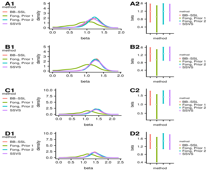
(a) Active predictors, from top to bottom: $\beta_{1},\beta_{4},\beta_{7},\beta_{10}$

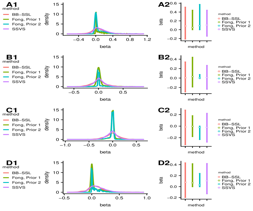
(b) Inactive predictors, from top to bottom: $\beta_{2},\beta_{5},\beta_{8},\beta_{11}$

Figure 11: Comparison of Fong et al. (2019)’s algorithm 2 with different choice of priors and loss function versus BB-SSL and SSVS under simulated dataset. We use $n=50,p=12$, $\boldsymbol{\beta}=(1.3,0,0,1.3,0,0,1.3,0,0,1.3,0,0)^{T}$, predictors are grouped into 4 blockes with correlation coefficient $\rho=0.6$, $\alpha=2$, $m=50$, $c=10$, $\lambda_{0}=7,\lambda_{1}=0.15$.

Appendix C Another Gibbs Sampler with Complexity $O(np)$

A referee suggested a one-site Gibbs sampler which can be implemented with our continuous Spike-and-Slab LASSO prior and which can potentially improve computational efficiency. The sampler is reminiscent of Geweke (1996) who proposed a variant for point mass spikes to avoid getting stuck after generating $\beta_{i}=0$. However, although George and McCulloch (1997) mentioned that this implementation might also be useful under continuous spike-and-slab priors (where the variance ratio of slab to spike is large), we find this implementation to be rarely used for continuous priors. One-site Gibbs samplers are expected to converge slower and yield higher autocorrelation, which is one of the reasons why block-Gibbs samplers have been preferred. We nevertheless explore this Gibbs sampler further.

The algorithm to implement Geweke (1996)’s Gibbs sampler for the Spike-and-Slab LASSO prior is outlined in Algorithm 4 and we further refer to it as Gibbs II. We calculate the vector $\boldsymbol{r}_{j}$ through $\boldsymbol{r}_{j}=(\boldsymbol{y}-\boldsymbol{X}\boldsymbol{\beta})+\boldsymbol{X}_{j}\beta_{j}$ and $\boldsymbol{y}-\boldsymbol{X}\boldsymbol{\beta}$ is calculated once before running MCMC and updated after each update on $\beta_{j}$. When $p>n$, Algorithm 4 has complexity $O(np)$ compared to $O(p^{3})$ for SSVS1 and $O(n^{2}p)$ for SSVS2. However, generating from the Truncated Normal distribution typically requires an accept-reject algorithm (Geweke, 1991) which creates some computational bottlenecks. We utilize the R package ‘truncnorm’ (Trautmann et al., 2015) which implements this accept-reject algorithm in C. The performance of Algorithm 4 against other methods is summarized in Table 4. We see that the per-iteration running time of Gibbs II is similar to SSVS2 (using the trick in Bhattacharya et al. (2016)), yet the serial correlation is higher than for both implementations of SSVS. Thus, contrary to the point-mass spike, Algorithm 4 (which is based on Geweke (1996)) trades computational efficiency for serial correlation. In general, the time used for generating the same number of effective samples is slightly longer than SSVS2, but improves significantly over SSVS1. From this observation, we believe Gibbs II is yet another useful method to speed up the standard SSVS1 under the Spike-and-Slab LASSO prior.

method	time per 100 iter (sec)	ESS per 100 iter	lag-one auto correlation on $\beta_{j}$’s	time per 100 ESS (sec)
BB-SSL	0.7	100	-0.002	0.7
SSVS1	40	98	0.006	40.82
SSVS2	3.2	98	0.006	3.27
Gibbs II	3.1	83	0.100	3.73

Table 4: Performance comparison of Algorithm 4 (referred to as Gibbs II) against other methods. We set $n=100,p=1000$, variables are equi-correlated with $\rho=0.9$, and the active coefficients are $\beta_{active}=(2,4,-4,6)^{\prime}$.

A less relevant, but perhaps interesting, observation is that since the Spike-and-Slab LASSO prior is a mixture of Laplace distributions, SSVS1 (which augments the data with $\tau_{j}$’s) can be seen as a generalization of the MCMC algorithm in Park and Casella (2008) while Gibbs II can be seen as a spike-and-slab version of the MCMC algorithm in Hans (2009). Our conclusion from this exercise is that, for the Spike-and-Slab LASSO prior, BB-SSL is actually doing better (both in terms of serial correlation and timing) compared with Gibbs II.

Set: $\lambda_{0}\gg\lambda_{1},$ $a,b>0$, $T$ (number of MCMC iterations), $B$ (number of samples to discard as burn-in).

Initialize: $\boldsymbol{\beta}^{0}$ (e.g. LASSO solution after 10-fold cross validation) and $\boldsymbol{\tau}^{0}$.

for $t=1,2,\cdots,T$ do

       for $j=1,2,\cdots,p$ do

             (a) Sample $\gamma_{j}\sim\pi\left(\gamma_{j}|\theta,\boldsymbol{\beta}_{-j},\boldsymbol{\gamma}_{-j},\boldsymbol{y}\right)=\text{Bernoulli}\left(\frac{\pi_{1}}{\pi_{1}+\pi_{0}}\right)$, where

$$\pi_{1}=\theta c_{1},\quad\pi_{0}=(1-\theta)c_{0},$$

$$c_{1}=\lambda_{1}\left[e^{(\mu^{1}_{+})^{2}/(2s_{j})}\mathbb{P}\left(N(\mu_{+}^{1},s_{j})\geq 0\right)+e^{(\mu^{1}_{-})^{2}/(2s_{j})}\mathbb{P}\left(N(\mu_{-}^{1},s_{j})\leq 0\right)\right],$$

$$c_{0}=\lambda_{0}\left[e^{(\mu^{0}_{+})^{2}/(2s_{j})}\mathbb{P}\left(N(\mu_{+}^{0},s_{j})\geq 0\right)+e^{(\mu^{0}_{-})^{2}/(2s_{j})}\mathbb{P}\left(N(\mu_{-}^{0},s_{j})\leq 0\right)\right],$$

$$\mu_{-}^{1}=\frac{\boldsymbol{r}_{j}^{T}\boldsymbol{X}_{j}+\sigma^{2}\lambda_{1}}{\|\boldsymbol{X}_{j}\|_{2}^{2}},\quad\mu_{+}^{1}=\frac{\boldsymbol{r}_{j}^{T}\boldsymbol{X}_{j}-\sigma^{2}\lambda_{1}}{\|\boldsymbol{X}_{j}\|_{2}^{2}},\quad\boldsymbol{r}_{j}=\boldsymbol{y}-\sum_{k\neq j}\boldsymbol{X}_{k}\beta_{k},$$

$$\mu_{-}^{0}=\frac{\boldsymbol{r}_{j}^{T}\boldsymbol{X}_{j}+\sigma^{2}\lambda_{0}}{\|\boldsymbol{X}_{j}\|_{2}^{2}},\quad\mu_{+}^{0}=\frac{\boldsymbol{r}_{j}^{T}\boldsymbol{X}_{j}-\sigma^{2}\lambda_{0}}{\|\boldsymbol{X}_{j}\|_{2}^{2}},\quad s_{j}=\sigma^{2}\|\boldsymbol{X}_{j}\|_{2}^{-2}.$$

(b) Sample $\beta_{j}\sim\pi(\beta_{j}|\gamma_{j},\theta,\boldsymbol{\beta}_{-j},\boldsymbol{\gamma}_{-j},\boldsymbol{y})=u_{0}\text{TruncNormal}^{-}\left(\mu_{-}^{\gamma_{j}},s_{j}\right)+(1-u_{0})\text{TruncNormal}^{+}\left(\mu_{+}^{\gamma_{j}},s_{j}\right)$ where

$$u_{0}=\frac{\mathbb{P}\left(N(\mu_{-}^{\gamma_{j}},s_{j})\leq 0\right)}{\mathbb{P}\left(N(\mu_{-}^{\gamma_{j}},s_{j})\leq 0\right)+\mathbb{P}\left(N(\mu_{+}^{\gamma_{j}},s_{j})\geq 0\right)\exp\left\{-\frac{2\boldsymbol{r}_{j}^{T}\boldsymbol{X}_{j}\lambda_{\gamma_{j}}}{\|\boldsymbol{X}_{j}\|^{2}_{2}}\right\}},$$

$$\text{TruncNormal}^{-}(\mu,s)=\mathbb{P}\left(X\mid X\leq 0\right)\quad\text{where}\quad X\sim N(\mu,s),$$

$$\text{TruncNormal}^{+}(\mu,s)=\mathbb{P}\left(X\mid X\geq 0\right)\quad\text{where}\quad X\sim N(\mu,s).$$

       end for

      (c) Sample $\theta\sim\mathrm{Beta}(\sum_{j=1}^{p}\gamma_{j}+a,p-\sum_{j=1}^{p}\gamma_{j}+b)$.

      

end for

Return: $\boldsymbol{\beta}^{t},\boldsymbol{\gamma}^{t},\theta^{t}$ where $t=B+1,B+2,\cdots,T$.

Algorithm 4 Gibbs II

Appendix D Details on Computational Complexity Analysis

Below are details for the computational complexity analysis as shown in Table 1 of the main text.

BB-SSL, WBB1, WBB2.

BB-SSL uses R package SSLASSO (Ročková and Moran (2017)) to implement the coordinate-descent algorithm in Ročková and George (2018). It iteratively updates $\boldsymbol{\beta}$ until convergence. At each iteration, we first update the active coordinates, then the candidate coordinates, and finally the inactive coordinates. The total number of iterations is limited to a pre-defined number. There are two ways to update each coordinate, one way is to keep track of a residual vector and for each coordinate we compute the inner product between the residual vector and $\boldsymbol{X}_{j}$ – this takes $O(n)$; another way is to pre-compute the Gram matrix and for each coordinate, we calculate the inner product between $\boldsymbol{X}^{T}\boldsymbol{X}_{j}$ and $\hat{\boldsymbol{\beta}}$ – this takes $O(p)$. For both ways, we update $\theta$ every $c$ iterations where each update is $O(p)$. So for a single value of $\lambda_{0}$, SSLASSO is $O(\min(\text{maxiter}\times p(n+\frac{p}{c_{1}}),\,(n+\text{maxiter})\times p^{2}))$. For a sequence of $\lambda_{0}$’s, complexity is $O(L\times\min(\text{maxiter}\times p(n+\frac{p}{c_{1}}),\,(n+\text{maxiter})\times p^{2}))$ where $L$ is the length of $\lambda_{0}$’s. Usually if the biggest $\lambda_{0}$ is large enough, we would expect that the larger $\lambda_{0}$’s can reach convergence quickly using the estimated $\boldsymbol{\beta}$ from previous $\lambda_{0}$’s, so usually it takes less than $O\left(L\times\min\left(\text{maxiter}\times p(n+\frac{p}{c_{1}}),\,(n+\text{maxiter})\times p^{2}\right)\right)$.

SSVS1.

The computational complexity for Algorithm 1 is $O(p^{3})$ per iteration when $p>n$. Under this setting, we use the Woodbury matrix identity to simplify the matrix multiplication $(\boldsymbol{X}^{T}\boldsymbol{X}+\boldsymbol{D}_{\tau}^{-1})^{-1}=\boldsymbol{D}_{\tau}-\boldsymbol{D}_{\tau}\boldsymbol{X}^{T}(\boldsymbol{I}_{n}+\boldsymbol{X}\boldsymbol{D}_{\tau}\boldsymbol{X}^{T})^{-1}\boldsymbol{X}\boldsymbol{D}_{\tau}$, whose complexity is $O(p^{2}n)$.

SSVS2.

Using Bhattacharya et al. (2016)’s matrix inversion formula to generate the $p$-dimensional multivatiate Gaussian takes $O(n^{2}p+n^{3})=O(n^{2}\max(n,p))$.

Skinny Gibbs.

We modified Skinny Gibbs to sample from the posterior using SSL prior. Theoretically it is of complexity $O(np)$. However, sometimes when $n$ is relatively small, we observe that the running time of Skinny Gibbs is slower than Bhattacharya’s method. This is because Skinny Gibbs involves an $O(n)$ matrix product for each coordinate and the update for each coordinate is implemented via for-loop, whereas in Bhattacharya’s method the $O(n^{2}p)$ operation is one matrix product which is very efficiently optimized in R. We will see that as $n$ increases, this problem diminishes and Skinny Gibbs becomes faster than Bhattacharya’s method.

WLB.

Generating each WLB sample involves solving a least square problem whose complexity is $O(p^{2}n)$ when $p\leq n$. WLB is not applicable when $p>n$.

Appendix E Additional Experimental Results

E.1 Low Dimensional Setting

When all covariates are mutually independent, we first investigate the marginal density of $\beta_{i}$’s, which is shown in Figure 12. We find that all methods perform well for active $\beta_{i}$’s. WBB1 and WBB2 are doing poorly for inactive $\beta_{i}$’s. For the marginal mean of $\gamma_{i}$’s, as shown in Figure 13, all methods perform well. All methods can detect over 95% of models. In Table 5, we quantify the performance of each method in the low-dimensional setting. In the settings we tried, BB-SSL consistently has the best performance.

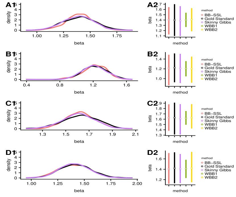
(a) Active predictors, from top to bottom: $\beta_{1},\beta_{4},\beta_{7},\beta_{10}$

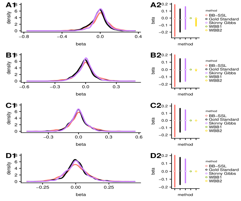
(b) Inactive predictors, from top to bottom: $\beta_{2},\beta_{5},\beta_{8},\beta_{11}$

Figure 12: Estimated posterior density (left panel) and credible intervals (right panel) of $\beta_{i}$’s in the low-dimensional independent case. We have $n=50,p=12,\beta_{active}=(1.3,1.3,1.3,1.3)^{\prime},\lambda_{0}=7,\lambda_{1}=0.15,\rho=0$. Each method has $5\,000$ sample points (after thinning for SSVS and Skinny Gibbs). BB-SSL is fitted using a single value $\lambda_{0}=7$. Since WBB1 and WBB2 produce a point mass at zero, we exclude them from density comparisons.

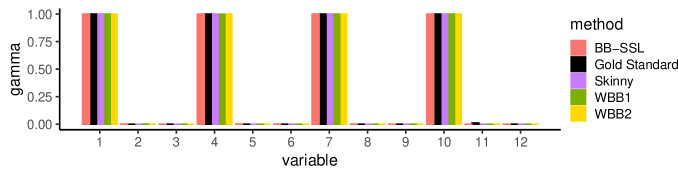
Figure 13: Mean of $\gamma_{i},i=1,2,\cdots,12$ in low-dimensional, independent case. $n=50,p=12,\beta_{active}=(1.3,1.3,1.3,1.3)$ and predictors mutually independent. Each method is (thinned to) 1,000 sample points. $\lambda_{0}=13,\lambda_{1}=0.05$. SSLASSO is fitted using a single $\lambda_{0}$.

Setting	Block-wise $\rho=0.6$, $\beta_{active}=(1.3,1.3,1.3,1.3)^{\prime}$									Block-wise $\rho=0.9$, $\beta_{active}=(1.3,1.3,1.3,1.3)^{\prime}$
Metric	$\beta_{j}$’s						$\gamma_{j}$’s		Model	$\beta_{j}$’s						$\gamma_{j}$’s		Model
Metric	KL		JD of 90% CI		‘Bias’		‘Bias’		HD	KL		JD of 90% CI		‘Bias’		‘Bias’		HD
	$+$	$-$	$+$	$-$	$+$	$-$	$+$	$-$	all	$+$	$-$	$+$	$-$	$+$	$-$	$+$	$-$	all
Skinny Gibbs	0.24	0.25	0.29	0.34	0.08	0.07	0.02	0.0007	0	0.68	0.33	0.37	0.39	0.15	0.08	0.04	0.009	0.2
WBB1	0.22	1.66	0.28	0.62	0.09	0.04	0.02	0.0004	0	0.67	2.73	0.41	0.89	0.14	0.08	0.05	0.003	0.2
WBB2	0.20	1.69	0.28	0.62	0.08	0.04	0.02	0.0004	0	0.56	2.69	0.33	0.87	0.14	0.07	0.05	0.003	0.2
BB-SSL	0.15	0.07	0.21	0.24	0.09	0.03	0.02	0.0003	0	0.14	0.09	0.21	0.24	0.13	0.07	0.04	0.002	0.2
Setting	Equi-correlation $\rho=0.6$, $\beta_{active}=(1.3,1.3,1.3,1.3)^{\prime}$									Equi-correlation $\rho=0.9$, $\beta_{active}=(1,1.5,-1.5,2)^{\prime}$
Metric	$\beta_{j}$’s						$\gamma_{j}$’s		Model	$\beta_{j}$’s						$\gamma_{j}$’s		Model
Metric	KL		JD of 90% CI		‘Bias’		‘Bias’		HD	KL		JD of 90% CI		‘Bias’		‘Bias’		HD
	$+$	$-$	$+$	$-$	$+$	$-$	$+$	$-$	all	$+$	$-$	$+$	$-$	$+$	$-$	$+$	$-$	all
Skinny Gibbs	0.11	0.20	0.20	0.31	0.06	0.06	0.05	0.002	0.2	0.66	0.29	0.27	0.40	0.30	0.06	0.01	0.016	1
WBB1	0.15	1.97	0.22	0.75	0.09	0.05	0.02	0.001	0.2	1.18	2.72	0.37	0.88	0.14	0.06	0.01	0.001	0.2
WBB2	0.14	1.98	0.23	0.75	0.09	0.05	0.02	0.001	0.2	1.20	2.70	0.37	0.87	0.14	0.05	0.01	0.001	0.2
BB-SSL	0.10	0.07	0.19	0.24	0.08	0.03	0.02	0.002	0.2	0.23	0.07	0.51	0.20	0.12	0.05	0.01	0.001	0.2

Table 5: Evaluation of approximation properties (relative to SSVS) in the low-dimensional setting with $n=50$ and $p=12$ based on 10 independent runs. We set $\lambda_{0}=7,\lambda_{1}=0.15$. The best performance is marked in bold font. KL is the Kullback-Leibler divergence, JD is the Jaccard distance of credible intervals (CI), HD is the Hamming distance of the median models. ‘Bias’ refers to the $l_{1}$ distance of estimated posterior means. We denote with $*$ all numbers smaller than 0.0001, with $+$ an average over active coordinates, and with $-$ an average over inactive coordinates.

E.2 High Dimensional, Block-wise Correlation Structure

Figure 14 shows the posterior for $\beta_{i}$’s when $\rho=0$, Figure 15 is for $\rho=0.6$ and Figure 16 is for $\rho=0.9$ in the block-wise correlated setting. Skinny Gibbs slightly underestimates the variance for active coordinates. WBB1 and WBB2 does poorly for inactive coordinates. In general BB-SSL does well. Figure 17(a) shows the marginal inclusion probabilities (MIP) when $\rho=0.6$ ($\rho=0,0.9$ are included in the main text) and we see that all methods perform well except that Skinny Gibbs sometimes overestimates MIP.

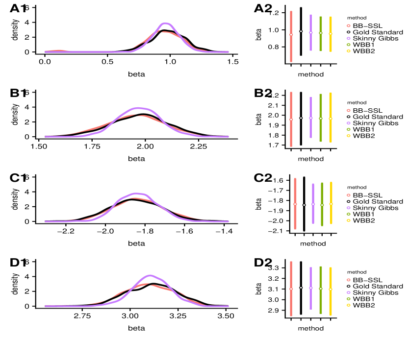
(a) Active predictors, from top to bottom: $\beta_{1},\beta_{11},\beta_{21},\beta_{31}$

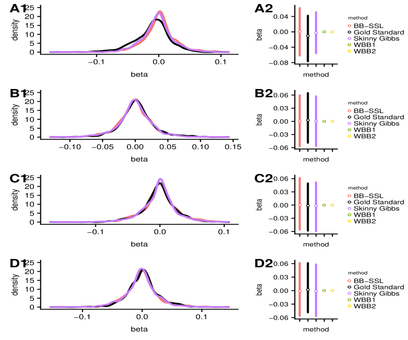
(b) Inactive predictors, from top to bottom: $\beta_{2},\beta_{12},\beta_{22},\beta_{32}$

Figure 14: Estimated posterior density (left panel) and credible intervals (right panel) of $\beta_{i}$’s in the high-dimensional independent case ($\rho=0$). We have $n=100,p=1000,\beta_{active}=(1,2,-2,3)^{\prime},\lambda_{0}=50,\lambda_{1}=0.05$. Each method has $5\,000$ sample points (after thinning for SSVS and Skinny Gibbs). BB-SSL is fitted using a single $\lambda_{0}$ and initialized at SSLASSO solution on the original $\boldsymbol{X},\boldsymbol{y}$. Since WBB1 and WBB2 produce a point mass at zero, we exclude them from density comparisons.

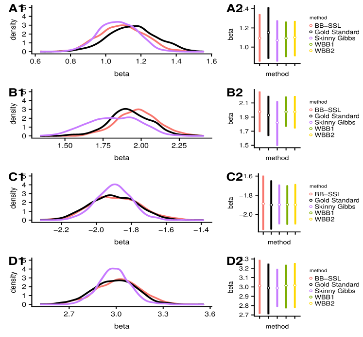
(a) Active predictors, from top to bottom: $\beta_{1},\beta_{11},\beta_{21},\beta_{31}$

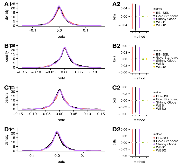
(b) Inactive predictors, from top to bottom: $\beta_{2},\beta_{12},\beta_{22},\beta_{32}$

Figure 15: Estimated posterior density (left panel) and credible intervals (right panel) of $\beta_{i}$’s in the high-dimensional block-wise correlated case ($\rho=0.6$). We have $n=100,p=1000,\beta_{active}=(1,2,-2,3)^{\prime},\lambda_{0}=50,\lambda_{1}=0.05$. Each method has $5\,000$ sample points (after thinning for SSVS and Skinny Gibbs). BB-SSL is fitted using a single $\lambda_{0}$ and initialized at SSLASSO solution on the original $\boldsymbol{X},\boldsymbol{y}$. Since WBB1 and WBB2 produce a point mass at zero, we exclude them from density comparisons.

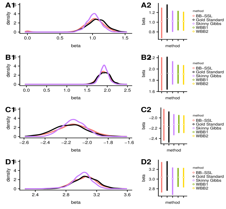
(a) Active predictors, from top to bottom: $\beta_{1},\beta_{11},\beta_{21},\beta_{31}$

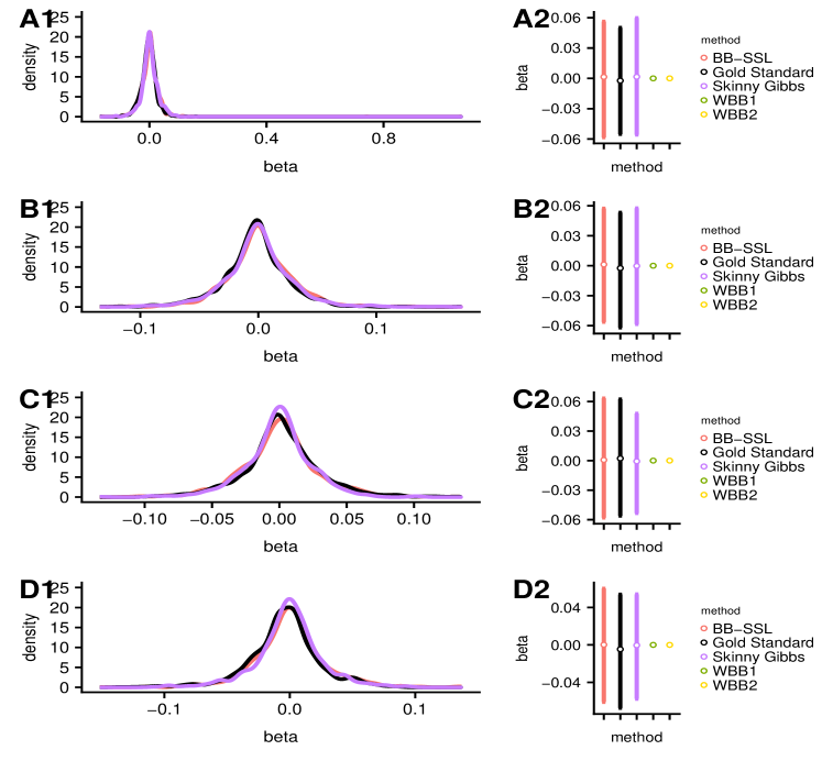
(b) Inactive predictors, from top to bottom: $\beta_{2},\beta_{12},\beta_{22},\beta_{32}$

Figure 16: Estimated posterior density (left panel) and credible intervals (right panel) of $\beta_{i}$’s in the high-dimensional, block-wise correlated case ($\rho=0.9$). We have $n=100,p=1000,\beta_{active}=(1,2,-2,3)^{\prime},\lambda_{0}=50,\lambda_{1}=0.05$. Each method has $5\,000$ sample points (after thinning for SSVS and Skinny Gibbs). BB-SSL is fitted using a single $\lambda_{0}$ and initialized at SSLASSO solution on the original $\boldsymbol{X},\boldsymbol{y}$. Since WBB1 and WBB2 produce a point mass at zero, we exclude them from density comparisons.

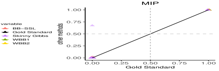
(a) Block-wise $\rho=0.6$

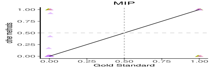
(b) Block-wise $\rho=0.99$

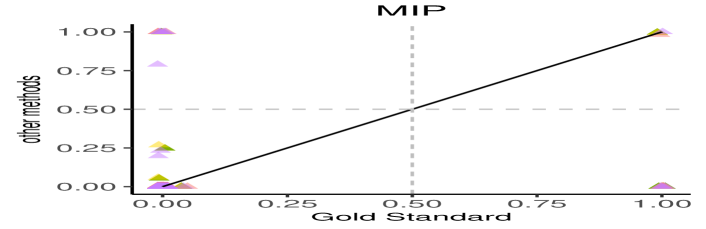
(c) Equi-correlation $\rho=0.9$

Figure 17: Posterior means of $\gamma_{i}$’s (i.e. a marginal inclusion probabilities) in high-dimensional settings with $n=100,p=1000$. We set $\lambda_{0}=50,\lambda_{1}=0.05$.

In the more extreme case where $\rho=0.99$, SSVS suffers severely from local entrapment with the signal $\beta_{active}=(1,2,-2,3)^{\prime}$, so we set a stronger signal with $\beta_{active}=(2,4,-4,6)^{\prime}$. All the other settings are the same as before. We run two SSVS chains, one initialized at the truth and the other at origin. In Figure 18, we observe discrepancies in the posterior approximation for the two chains. This is why SSVS may not be a reliable gold standard to make comparisons with. We nevertheless observe that BB-SSL is close to the SSVS approximation obtained by initialization at the truth. Figure 17(b) shows the MIP and no method performs perfect in this extreme setting.

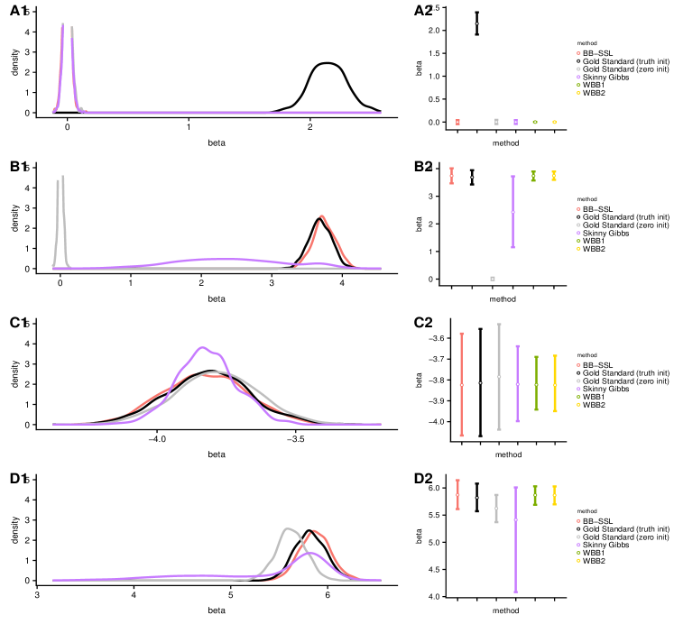
(a) Active predictors, from top to bottom: $\beta_{1},\beta_{11},\beta_{21},\beta_{31}$

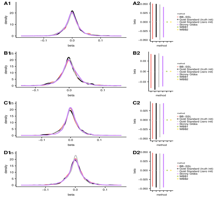
(b) Inactive predictors, from top to bottom: $\beta_{2},\beta_{12},\beta_{22},\beta_{32}$

Figure 18: Estimated posterior density (left panel) and credible intervals (right panel) of $\beta_{i}$’s in the high-dimensional block-wise correlated case ($\rho=0.99$). We have $n=100,p=1000,\beta_{active}=(2,4,-4,6)^{\prime},\lambda_{0}=50,\lambda_{1}=0.05$. Each method has $5\,000$ sample points (after thinning for SSVS and Skinny Gibbs). BB-SSL is fitted using a single $\lambda_{0}$ and initialized at SSLASSO solution on the original $\boldsymbol{X},\boldsymbol{y}$. Since WBB1 and WBB2 produce a point mass at zero, we exclude them from density comparisons.

E.3 High Dimensional, Equi-correlation Structure

When all covariates are equi-correlated with $\rho=0.9$, SSVS appears to suffer severely from a local trap when $\beta_{0}=2,\beta_{2}=3,\beta_{3}=-3$ and $\beta_{4}=4$. Thus, we also try a setting with larger signals $\beta_{0}=2,\beta_{2}=4,\beta_{3}=-4$ and $\beta_{4}=6$. Results for the smaller signal $\beta_{active}=(2,3,-3,4)^{\prime}$ are summarized in Figure 19 and results for the larger signal $\beta_{active}=(2,4,-4,6)^{\prime}$ are in Figure 20. We show results for both SSVS initializations (one at original and the other at the truth) and observe discrepancies in the posterior approximation. This is why SSVS may not be a reliable gold standard to make comparisons with. We nevertheless observe that BB-SSL is close to the SSVS approximation obtained by initialization at the truth.

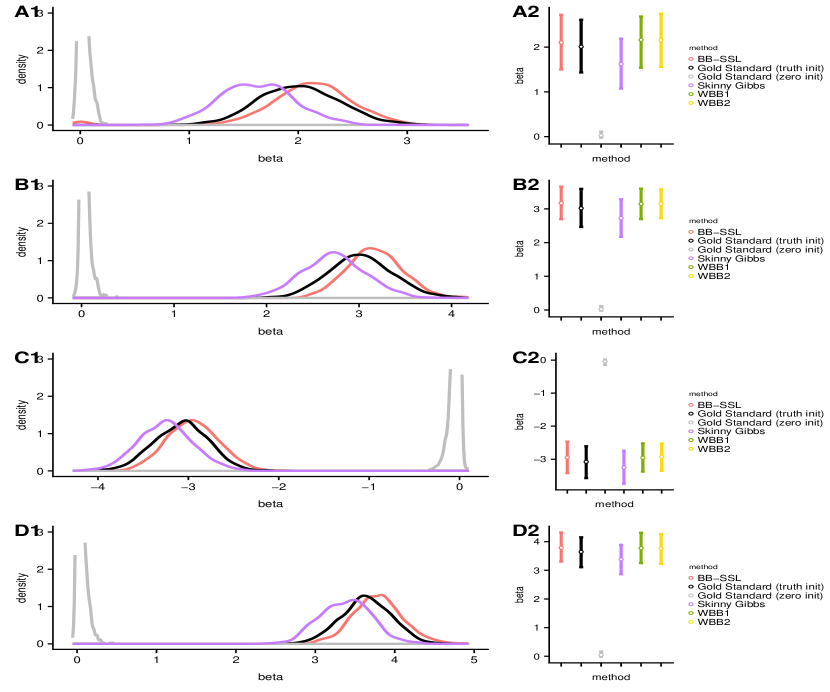
(a) Active predictors, from top to bottom: $\beta_{1},\beta_{2},\beta_{3},\beta_{4}$

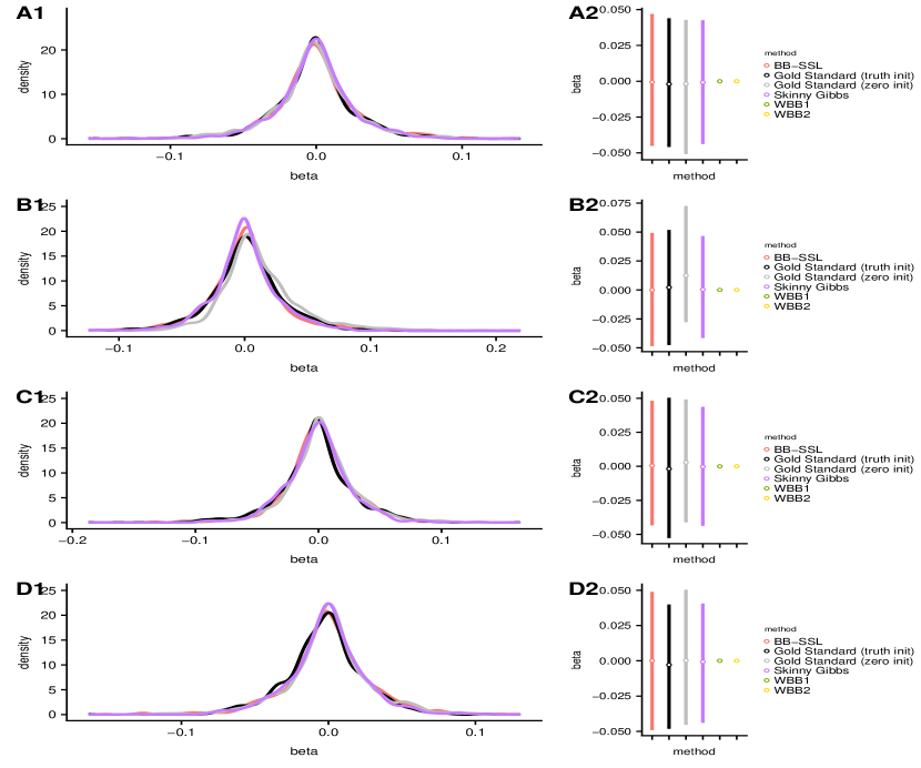
(b) Inactive predictors, from top to bottom: $\beta_{5},\beta_{6},\beta_{7},\beta_{8}$

Figure 19: Estimated posterior density (left panel) and $90\%$ credible intervals (right panel) of $\beta_{i}$’s when all covariatess are correlated with $\rho=0.9$.

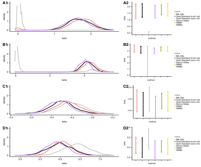
(a) Active predictors, from top to bottom: $\beta_{1},\beta_{2},\beta_{3},\beta_{4}$

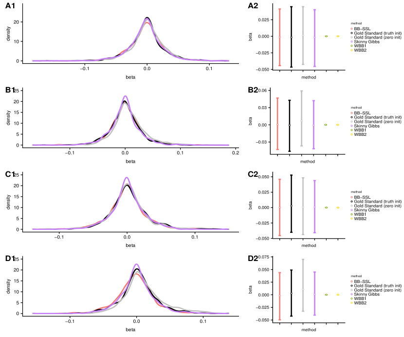
(b) Inactive predictors, from top to bottom: $\beta_{5},\beta_{6},\beta_{7},\beta_{8}$

Figure 20: Estimated posterior density (left panel) and $90\%$ credible intervals (right panel) of $\beta_{i}$’s when all covariatess are correlated with $\rho=0.9$.

E.4 Influence of $\alpha$ On The Posterior

In this section we investigate the influence of $\alpha$ on BB-SSL posterior under (a) high-dimensional, block-wise correlated ($\rho=0.6$) setting, as shown in Figure 21, and (b) Durable Goods Marketing Data Set, as shown in Figure 22. In both datasets, as we increase $\alpha$, the change in posterior variance reduces for each unit increase in $\alpha$.

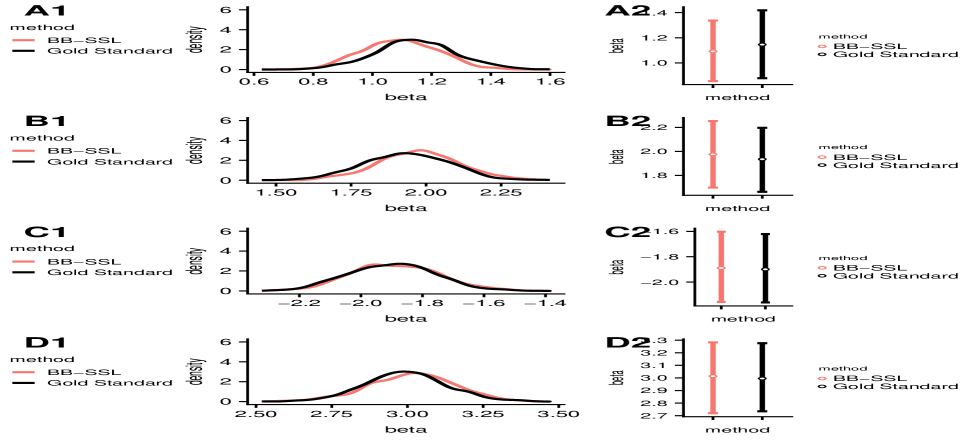
(a) $\alpha=2$.

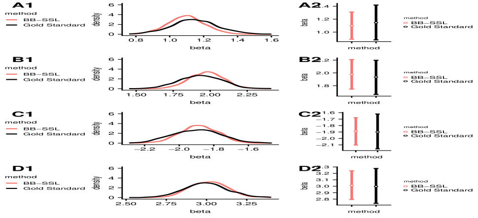
(b) $\alpha=10$.

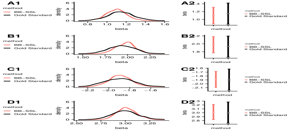
(c) $\alpha=100$.

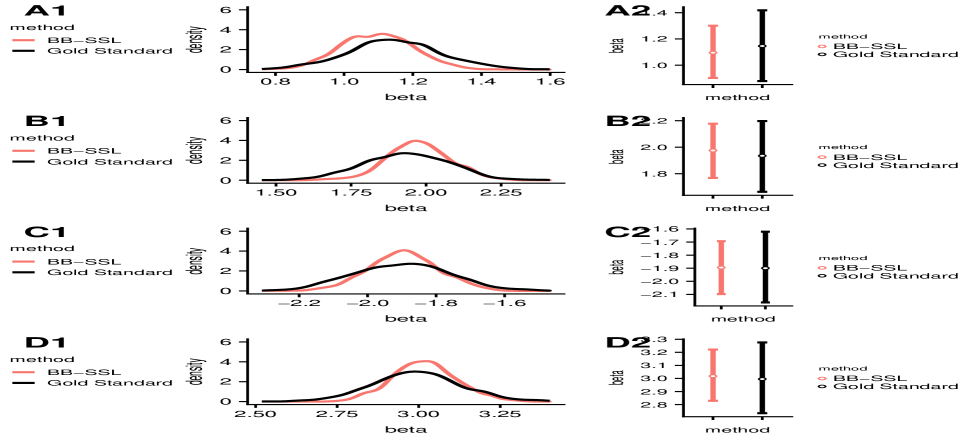
(d) $\alpha=1000$.

Figure 21: Comparison of posterior density for active $\beta_{i}$’s when choosing different $\alpha$ in high-dimensional, block-wise correlated setting ($\rho=0.6$). SSLASSO is fitted with $\lambda_{0}$ being an equal difference sequence of length 10 starting at 0.05 and ending at 50. We set $\lambda_{1}=0.05$. Since WBB1 and WBB2 produce a point mass and do not fit into the $y$-axis, we exclude it in the density plot.

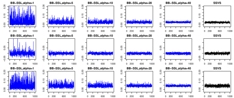
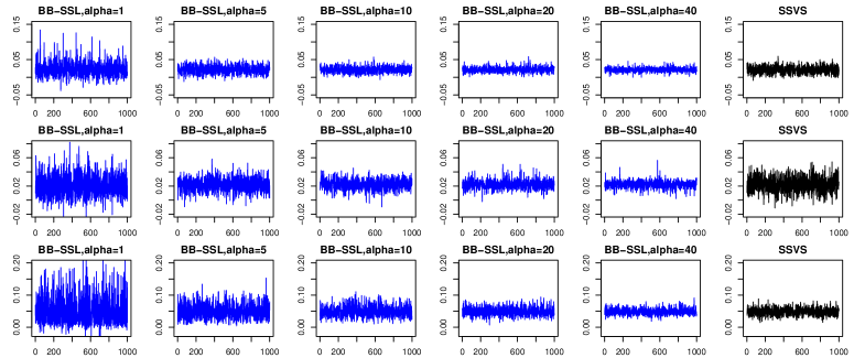
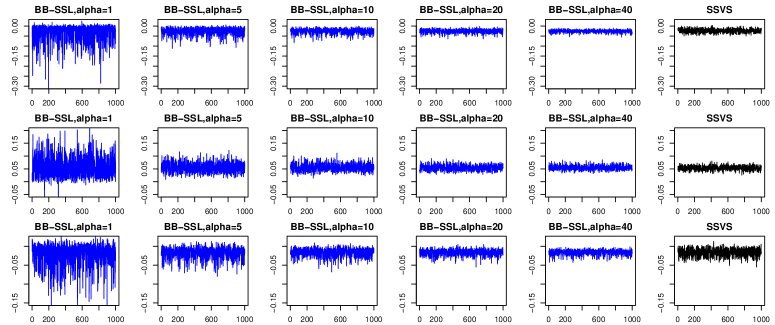
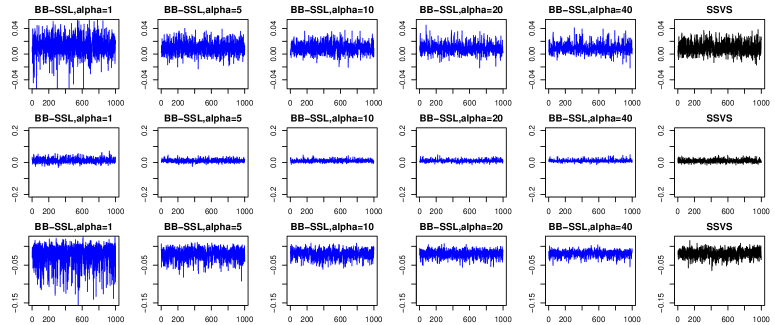
Figure 22: Trace plots of $\beta_{i},i,1,2,\cdots,12$ under varying $\alpha$’s in model (19) in the Durable Goods Marketing Data Set.

References

- Ando and Modigliani (1963) Ando, A. and Modigliani, F. (1963). The “life cycle” hypothesis of saving: Aggregate implications and tests. The American Economic Review, 53(1):55–84.
- Bai et al. (2020) Bai, R., Moran, G. E., Antonelli, J. L., Chen, Y., and Boland, M. R. (2020). Spike-and-slab group lassos for grouped regression and sparse generalized additive models. Journal of the American Statistical Association (to appear).
- Belsley et al. (2005) Belsley, D. A., Kuh, E., and Welsch, R. E. (2005). Regression diagnostics: Identifying influential data and sources of collinearity, volume 571. John Wiley & Sons.
- Beygelzimer et al. (2013) Beygelzimer, A., Kakadet, S., Langford, J., Arya, S., Mount, D., and Li, S. (2013). FNN: fast nearest neighbor search algorithms and applications. R package version, 1(1).
- Bhattacharya et al. (2016) Bhattacharya, A., Chakraborty, A., and Mallick, B. K. (2016). Fast sampling with Gaussian scale mixture priors in high-dimensional regression. Biometrika, 103(4):985.
- Bhattacharya et al. (2015) Bhattacharya, A., Pati, D., Pillai, N. S., and Dunson, D. B. (2015). Dirichlet–Laplace priors for optimal shrinkage. Journal of the American Statistical Association, 110(512):1479–1490.
- Bottolo and Richardson (2010) Bottolo, L. and Richardson, S. (2010). Evolutionary stochastic search for Bayesian model exploration. Bayesian Analysis, 5(3):583–618.
- Carbonetto and Stephens (2012) Carbonetto, P. and Stephens, M. (2012). Scalable variational inference for Bayesian variable selection in regression, and its accuracy in genetic association studies. Bayesian Analysis, 7(1):73–108.
- Carvalho et al. (2010) Carvalho, C. M., Polson, N. G., and Scott, J. G. (2010). The horseshoe estimator for sparse signals. Biometrika, 97(2):465–480.
- Clyde et al. (2011) Clyde, M. A., Ghosh, J., and Littman, M. L. (2011). Bayesian adaptive sampling for variable selection and model averaging. Journal of Computational and Graphical Statistics, 20(1):80–101.
- Deshpande et al. (2019) Deshpande, S. K., Ročková, V., and George, E. I. (2019). Simultaneous variable and covariance selection with the multivariate spike-and-slab lasso. Journal of Computational and Graphical Statistics, 28(4):921–931.
- Efron (2012) Efron, B. (2012). Bayesian inference and the parametric bootstrap. The Annals of Applied Statistics, 6(4):1971.
- Fong et al. (2019) Fong, E., Lyddon, S., and Holmes, C. (2019). Scalable nonparametric sampling from multimodal posteriors with the posterior bootstrap. In International Conference on Machine Learning, pages 1952–1962.
- George and McCulloch (1993) George, E. I. and McCulloch, R. E. (1993). Variable selection via Gibbs sampling. Journal of the American Statistical Association, 88(423):881–889.
- George and McCulloch (1997) George, E. I. and McCulloch, R. E. (1997). Approaches for Bayesian variable selection. Statistica Sinica, 7(2):339–373.
- Geweke (1991) Geweke, J. (1991). Efficient simulation from the multivariate normal and student-t distributions subject to linear constraints and the evaluation of constraint probabilities. In Computing science and statistics: Proceedings of the 23rd symposium on the interface, pages 571–578.
- Geweke (1996) Geweke, J. (1996). Variable selection and model comparison in regression. In Bayesian Statistics 5.
- Hans (2009) Hans, C. (2009). Bayesian lasso regression. Biometrika, 96(4):835–845.
- Ishwaran and Rao (2005) Ishwaran, H. and Rao, J. S. (2005). Spike and slab gene selection for multigroup microarray data. Journal of the American Statistical Association, 100(471):764–780.
- Jaccard (1912) Jaccard, P. (1912). The distribution of the flora in the alpine zone. 1. New Phytologist, 11(2):37–50.
- Johndrow et al. (2020) Johndrow, J. E., Orenstein, P., and Bhattacharya, A. (2020). Bayes shrinkage at GWAS scale: Convergence and approximation theory of a scalable MCMC algorithm for the horseshoe prior. Journal of Machine Learning Research (to appear).
- Johnson and Rossell (2012) Johnson, V. E. and Rossell, D. (2012). Bayesian model selection in high-dimensional settings. Journal of the American Statistical Association, 107(498):649–660.
- Li et al. (2019) Li, Z., Mccormick, T., and Clark, S. (2019). Bayesian joint spike-and-slab graphical lasso. In International Conference on Machine Learning, pages 3877–3885.
- Lyddon et al. (2018) Lyddon, S., Walker, S., and Holmes, C. C. (2018). Nonparametric learning from Bayesian models with randomized objective functions. In Advances in Neural Information Processing Systems, pages 2071–2081.
- Madigan and Raftery (1994) Madigan, D. and Raftery, A. E. (1994). Model selection and accounting for model uncertainty in graphical models using Occam’s window. Journal of the American Statistical Association, 89(428):1535–1546.
- Martin and Walker (2014) Martin, R. and Walker, S. G. (2014). Asymptotically minimax empirical Bayes estimation of a sparse normal mean vector. Electronic Journal of Statistics, 8(2):2188–2206.
- Meyer et al. (2014) Meyer, D., Dimitriadou, E., Hornik, K., Weingessel, A., Leisch, F., Chang, C., and Lin, C. (2014). e1071: Misc functions of the department of statistics (e1071), TU Wien. R package version, 1(3).
- Mitchell and Beauchamp (1988) Mitchell, T. J. and Beauchamp, J. J. (1988). Bayesian variable selection in linear regression. Journal of the American Statistical Association, 83(404):1023–1032.
- Moran et al. (2019) Moran, G. E., Ročková, V., George, E. I., et al. (2019). Variance prior forms for high-dimensional Bayesian variable selection. Bayesian Analysis, 14(4):1091–1119.
- Narisetty et al. (2019) Narisetty, N. N., Shen, J., and He, X. (2019). Skinny Gibbs: A consistent and scalable Gibbs sampler for model selection. Journal of the American Statistical Association, 114(527):1205–1217.
- Newton et al. (2020) Newton, M. A., Polson, N. G., and Xu, J. (2020). Weighted Bayesian bootstrap for scalable posterior distributions. Canadian Journal of Statistics (In Press).