Accelerating MCMC algorithms through Bayesian Deep Networks

Abstract

Markov Chain Monte Carlo (MCMC) algorithms are commonly used for their versatility in sampling from complicated probability distributions. However, as the dimension of the distribution gets larger, the computational costsfor a satisfactory exploration of the sampling space become challenging. Adaptive MCMC methods employing a choice of proposal distribution can address this issue speeding up the convergence. In this paper we show an alternative way of performing adaptive MCMC, by using the outcome of Bayesian Neural Networks as the initial proposal for the Markov Chain. This combined approach increases the acceptance rate in the Metropolis-Hasting algorithm and accelerate the convergence of the MCMC while reaching the same final accuracy. Finally, we demonstrate the main advantages of this approach by constraining the cosmological parameters directly from Cosmic Microwave Background maps.

1 Introduction

Cosmological observations have significantly increased in the last decade allowing us to obtain a better description of the Universe. This task has been also achieved thanks to Bayesian inference methods allowing to derive constraints on the parameters of cosmological models from those observations Verde [2007]. Bayesian inference offers a way to learn the prediction task from data through the posterior distribution $p(\theta|d)\sim p(d|\theta)p(\theta)$; being $\theta$ a set of unknown parameters of interest, $d$ the data associated with a measurement, $p(\theta)$ the prior distribution that quantifies what we know about $\theta$ before observing any data, and $p(d|\theta)$ is the likelihood function. Computing the true posterior is generally intractable, and approximation methods must be implemented in order to perform Bayesian inference in practice. Two main techniques for this purpose are Variational Inference and Markov Chain Monte Carlo (MCMC) Graves [2011], Metropolis et al. [1953], Regier et al. [2018], Jain et al. [2018]. The former method although computationally faster, requires the approximation of the true posterior, while the latter has become one of the most popular methods for cosmological parameter estimation due to its advantage of being non-parametric and asymptotically exact. Classical MCMC methods draw samples sequentially according to a probabilistic algorithm that allows to scale linearly with the dimension of the parameter space Verde [2007]. However if the complexity of the model increases from the presence of "slow" parameters, nuisance parameters, foregrounds or parameter correlations, the sampling will exhibit a high numerical cost Lewis [2013]. Additionally, it is generally difficult to determine a convenient initial state for the system and an accurate criterion to determine the convergence of the Markov Chain. These practical issues compel MCMC practitioners to resort convergence diagnostic tools which demand to run MCMC for a very long time to obtain good solutions Dunkley et al. [2005]. In this work we show a preliminary approach to accelerate the convergence of MCMC by including in the bottom of it, the approximate distribution outcome of the deep neural network as a proposal for the Markov Chain. We show the advantages of this approach in constraining the cosmological parameters directly from Cosmic Microwave Background (CMB) maps.

2 Dataset and Network

Following Hortua et al. [2019], we use 50.000 images related to the CMB maps projected in $20\times 20\,$deg² patches in the sky for training the Bayesian Neural Network. These images have a dimensions (256,256,3), where the last channel stands for the Temperature (channel=0) and Polarization (channel=1,2), and each image corresponds to a specific set value of the cosmological parameters: dark matter density $\omega_{cdm}$, spectrum amplitude $A_{s}$, baryon density $\omega_{b}$, and the dark energy density parameter $\Omega_{\Lambda}$. The BNN was implemented in TensorFlow-Probability, and the same version of the VGG architecture along with the presence of Flipout as it was shown in Hortua et al. [2019] was used in this paper. Finally, we used the calibration method introduced in Hortua et al. [2020] where $\alpha$-divergence with $\alpha=1$ has been included at the top of the BNN. Results of the conditional distributions for the predicted parameters by our BNN vs standard MCMC methods are displayed in Fig. 1.

3 Method

MCMC algorithms are commonly used for sampling from complicated distributions. As the dimension of the distribution gets larger, the computational costs for a satisfactory exploration of the sampling space become challenging. Adaptive MCMC methods such as the choice of proposal distributions in the Metropolis-Hastings algorithms are designed to address this issue speeding up the convergence. However, a suitable class of distribution is almost never known in advance and the search for improved proposal distributions is often done manually, through trial and error, which can be difficult especially in high dimensions. The method shown in this paper can be seen as a novel way to perform adaptive MCMC in which the output distribution of the BNNs serves as a proposal distribution for the MCMC. As it was shown in the previous work of  Hortua et al. [2019], multi-channel BNNs, are able to break degeneracies among parameters and provide reliable results close to the desired conditional posterior. This distribution can be used as potential proposals to significantly improve the performance during parameter inference. MCMC experiments were run in the cobaya software Torrado and Lewis [2020], with the likelihood given by Verde [2007]

$$-\mathcal{L} \sim \sum_{l}(2l+1)\bigg{[}\ln\bigg{(}\frac{C_{l}^{BB}}{\hat{C}_{l}^{BB}}\bigg{(}\frac{C_{l}^{TT}C_{l}^{EE}-(C_{l}^{TE})^{2}}{\hat{C}_{l}^{TT}\hat{C}_{l}^{EE}-(\hat{C}_{l}^{TE})^{2}}\bigg{)}\bigg{)}$$ (1)

$$+ \frac{\hat{C}_{l}^{BB}}{C_{l}^{BB}}+\frac{\hat{C}_{l}^{TT}C_{l}^{EE}+C_{l}^{TT}\hat{C}_{l}^{EE}-2\hat{C}_{l}^{TE}C_{l}^{TE}}{C_{l}^{TT}C_{l}^{EE}-(C_{l}^{TE})^{2}}\bigg{]},$$

where $\hat{C}_{l}$ is the power spectrum of the CMB patches obtained with Lens-Tools Petri [2016], and $C_{l}$ the theoretical model. Cobaya accepts the cosmological parameters as input, compute $C_{l}$ via CLASS Blas_2011 and when the Markov chains have enough points to provide reasonable samples from the posterior distributions, the simulation stops and it return the chains. We run two MCMC experiments taking into account the power spectrum of the CMB maps. In the first MCMC experiments we used the full sky map, while in the second one, we computed the power spectra for CMB patches and used them as an input in cobaya package.

4 Results

Results of the conditional distributions for the predicted parameters are displayed in Fig. 1 where we compared the MCMC results with the calibrated BNNs (on the CMB patches described in Section 2).

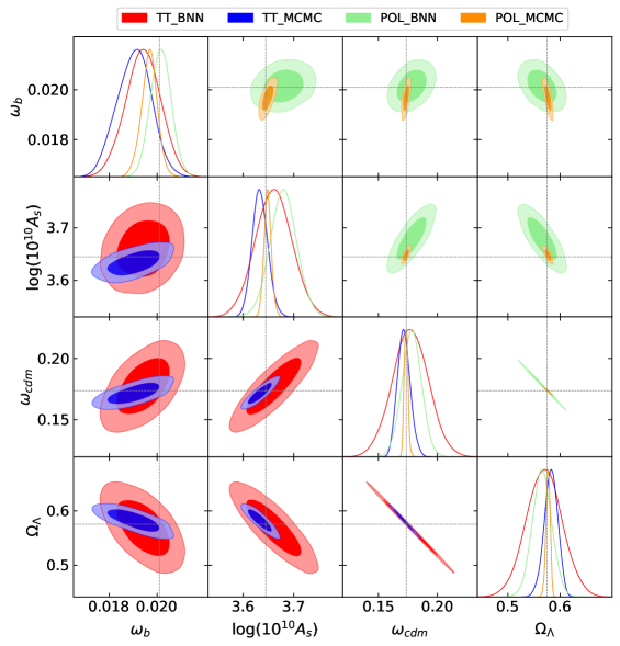
Figure 1: Marginalized parameter constraints obtained from temperature maps (TT) and combined temperature with polarization (POL) using MCMC and the best BNN model. The black line stand for the real value: $\omega_{b}=0.0201$, $\log(10^{10}A_{s})=3.6450$ and $\omega_{cdm}=0.1736$ taken from the test dataset.

Table 1: Statistics and Parameters $95\%$ intervals for the minimal base-$\Lambda$CDM model from our synthetic CMB dataset using non-informative priori (MCMC) and a precomputed covariance matrix from VI (covarBNN). The last column reports the metrics using the Full CMB map. The bold values in the last column correspond to the implementation of a proposal posterior distribution from VI. Although the full sky gives the smallest credible region, MCMC is 10000 times slower than VI. The real value considered is the same as specified in Fig. 1

Statistics for various MCMC sampling configurations
Metrics	Temperature map		Temperature+Polarization map
	MCMC	covarBNN	MCMC	covarBNN	Full-sky
$\omega_{b}$	$0.0190^{+0.0013}_{-0.0013}$	$0.0190^{+0.0012}_{-0.0012}$	$0.01967^{+0.00066}_{-0.00066}$	$0.01968^{+0.00064}_{-0.00064}$	$0.02009^{+0.00010}_{-0.00010}$
$\ln(10^{10}A_{s})$	$3.633^{+0.031}_{-0.031}$	$3.633^{+0.031}_{-0.030}$	$3.648^{+0.015}_{-0.015}$	$3.648^{+0.015}_{-0.016}$	$3.6449^{+0.0027}_{-0.0027}$
$\omega_{cdm}$	$0.171^{+0.011}_{-0.011}$	$0.170^{+0.011}_{-0.011}$	$0.1734^{+0.0031}_{-0.0032}$	$0.1734^{+0.0031}_{-0.0031}$	$0.1736^{+0.0009}_{-0.0009}$
$\Omega_{\Lambda}$	$0.583^{+0.025}_{-0.025}$	$0.583^{+0.024}_{-0.025}$	$0.5769^{+0.0079}_{-0.0080}$	$0.5769^{+0.0079}_{-0.0079}$	$0.5793^{+0.0019}_{-0.0019}$
Runtime	$4.02$hr	$1.56$hr	$4.40$hr	$3.14$hr	$4.52$hr//${\bf 3.15}$hr
Acc. rate	$0.19$	$0.23$	$0.14$	$0.25$	$0.18$//${\bf 0.23}$
$R-1$	$0.0093$	$0.0098$	$0.0051$	$0.0084$	$0.0091$//${\bf 0.0090}$
$(R-1)_{95\%CL}$	$0.0827$	$0.0764$	$0.0944$	$0.0642$	$0.0940$//${\bf 0.0800}$

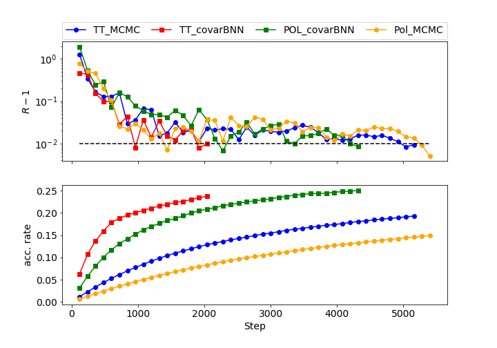
Figure 2: Graphical representation of convergence in MCMC using non-informative priori (MCMC) and a precomputed covariance matrix from VI (covarBNN). (Top) Gelman-Rubin values with respect to the acceptance step. (Bottom) Acceptance rate with respect the acceptance step. Notice that using a proposal covariance matrix takes shorter time for chains to converge.

We observe that MCMC provides tighter and more accurate constraints. However, the trained Neural Network can generate 8000 samples in approximately ten seconds which it turns out to be 10000 times faster than MCMC for this dataset . Runtime and metrics for convergence in MCMC are shown in Table 1. As expected, the polarization combined with temperature data shifts the values obtained from temperature alone and enhances the accuracy in all parameters (columns 1 and 3). Furthermore, a well-converged chain is also observed via the Gelman-Rubin $R-1$ parameter and its standard deviation at $95\%$ confidence level interval $(R-1)_{95\%CL}$ (the smaller the better). The qualitative correlations among parameters as obtained from BNNs are mostly analogous to the MCMC ones (Fig. 1), showing that a multi-channel BNN is able to handle the complexities involved in this kind of analysis and additionally to use the polarization information to break cosmological degeneracies. Nonetheless, although 10000 times slower, the MCMC it is able to better quantify the uncertainty. This is especially true when using the power spectrum of the full map, and the intervals are an order of magnitude more accurate than those computed by VI (rightmost column of Table 1). On the other hand, we can also combine MCMC and VI leveraging the advantages of both methods. Such topic has attracted a lot of attention in the recent literature Salimans et al. [2015], Thin et al. [2020]. A straightforward approach to speed up MCMC algorithms consists in using the covariance matrix constructed from the chains of the trained Neural Network as proposal for the distribution of the MCMC. In fact, it is known that a good estimate of the covariance matrix for the parameters increases the acceptance rate leading to significantly faster convergence Lewis [2013]. In Table 1, we compare the runtime for the MCMC with and without a precomputed covariance obtained from BNN. As we can see from the table, proposal covariances from BNNs (covarBNN) speed up convergence in MCMC reducing the computational time for all datasets (Temperature, Polarization and full sky maps). In Fig. 2 we report MCMC convergence diagnostic quantities such as $R-1$ and the acceptance rate per iteration. The stopping rule implemented in cobaya ensures that the Gelman-Rubin $R-1$ value and its standard deviation at $95\%$ confidence level interval $(R-1)_{95\%CL}$ computed from different chains (four in our case), satisfy the convergence criterion $R-1<0.01$ twice in a row, and $(R-1)_{95\%CL}<0.2$ respectively to stop the run, Torrado and Lewis [2020]. For the Temperature signal alone, the Markov chains achieve a steady state in about 2000 steps working with the covarBNN proposal while it usually takes more than 5000 steps instead with the vanilla MCMC. This behavior can also be explained by observing the acceptance rate in Fig. 2 (bottom), the red curve (TTcovarBNN) quickly approaches a considerably high acceptance rate, eventually converging at around 0.23 (which is a standard value for which we expect to have a decent acceptance rate Roberts et al. [1997]). An analogous trend can be seen for the polarization case.

5 Discussion

In this paper we show that MCMC algorithms excel at quantifying uncertainty with respect to BNNs models, although the latter is about 10000 times faster at inference. Given these properties, we showed an approach in which the covariance matrix efficiently estimated from the BNNs samples, significantly enhance the acceptance rate in MCMC yielding faster convergence. A limitation of this method is the use of partial CMB maps that prevent the access to large scales correlations, leading to large uncertainties and possibly introducing a bias in the prediction of the cosmological parameters sensible to such scales. It would be interesting (and more of a fair comparison) to compare MCMC for a full sky with respect to spherical neural architectures Krachmalnicoff and Tomasi [2019], Perraudin et al. [2019], cohen2018spherical which can extract large scale signals correlations, thus determining if Deep Learning methods can achieve a similar level of precision as compared with MCMC. As a future work, we also expect to assess the performance of this method with respect to other MCMC modifications such as a Hamiltonian Monte Carlo.

Broader Impact

Combining the speed of Bayesian Neural Networks with the accuracy of MCMC algorithms results in potential Bayesian inference methods for upcoming cosmological observation. Additionally, the network built in this work allows to adaptively extract complicated correlations when performing inference without assuming a priori summary statistics such as power spectrum or higher order spectra (such as bispectrum, trispectrum or others). This work presents an example for how machine learning could be used in the physics community to improve classical inference methods.

References

- Dunkley et al. [2005] J. Dunkley, M. Bucher, P. G. Ferreira, K. Moodley, and C. Skordis. Fast and reliable Markov chain Monte Carlo technique for cosmological parameter estimation. Monthly Notices of the Royal Astronomical Society, 356(3):925–936, 01 2005. ISSN 0035-8711. doi: 10.1111/j.1365-2966.2004.08464.x. URL https://doi.org/10.1111/j.1365-2966.2004.08464.x.
- Graves [2011] A. Graves. Practical variational inference for neural networks. In J. Shawe-Taylor, R. S. Zemel, P. L. Bartlett, F. Pereira, and K. Q. Weinberger, editors, Advances in Neural Information Processing Systems 24, pages 2348–2356. Curran Associates, Inc., 2011. URL http://papers.nips.cc/paper/4329-practical-variational-inference-for-neural-networks.pdf.
- Hortua et al. [2019] H. J. Hortua, R. Volpi, D. Marinelli, and L. Malagò. Parameters estimation for the cosmic microwave background with bayesian neural networks, 2019.
- Hortua et al. [2020] H. J. Hortua, L. Malago, and R. Volpi. Reliable uncertainties for bayesian neural networks using alpha-divergences. In Uncertainty and Robustness in Deep Learning Workshop, ICML, 2020.
- Jain et al. [2018] A. Jain, P. K. Srijith, and S. Desai. Variational inference as an alternative to mcmc for parameter estimation and model selection, 2018.
- Krachmalnicoff and Tomasi [2019] N. Krachmalnicoff and M. Tomasi. Convolutional Neural Networks on the HEALPix sphere: a pixel-based algorithm and its application to CMB data analysis. A& A, 628:A129, Aug 2019.
- Lewis [2013] A. Lewis. Efficient sampling of fast and slow cosmological parameters. Phys. Rev. D, 87:103529, May 2013. doi: 10.1103/PhysRevD.87.103529. URL https://link.aps.org/doi/10.1103/PhysRevD.87.103529.
- Metropolis et al. [1953] N. Metropolis, A. W. Rosenbluth, M. N. Rosenbluth, A. H. Teller, and E. Teller. Equation of state calculations by fast computing machines. The Journal of Chemical Physics, 21(6):1087–1092, 1953. doi: 10.1063/1.1699114. URL https://doi.org/10.1063/1.1699114.
- Perraudin et al. [2019] N. Perraudin, M. Defferrard, T. Kacprzak, and R. Sgier. DeepSphere: Efficient spherical Convolutional Neural Network with HEALPix sampling for cosmological applications. Astron. Comput., 27:130–146, 2019. doi: 10.1016/j.ascom.2019.03.004.
- Petri [2016] A. Petri. Mocking the weak lensing universe: The LensTools Python computing package. Astronomy and Computing, 17:73–79, Oct. 2016. doi: 10.1016/j.ascom.2016.06.001.
- Regier et al. [2018] J. Regier, A. C. Miller, D. Schlegel, R. P. Adams, J. D. McAuliffe, and Prabhat. Approximate inference for constructing astronomical catalogs from images, 2018.
- Roberts et al. [1997] G. O. Roberts, A. Gelman, and W. R. Gilks. Weak convergence and optimal scaling of random walk metropolis algorithms. Ann. Appl. Probab., 7(1):110–120, 02 1997. doi: 10.1214/aoap/1034625254. URL https://doi.org/10.1214/aoap/1034625254.
- Salimans et al. [2015] T. Salimans, D. P. Kingma, and M. Welling. Markov chain monte carlo and variational inference: Bridging the gap. In Proceedings of the 32nd International Conference on International Conference on Machine Learning - Volume 37, ICML’15, page 1218–1226. JMLR.org, 2015.
- Thin et al. [2020] A. Thin, N. Kotelevskii, J.-S. Denain, L. Grinsztajn, A. Durmus, M. Panov, and E. Moulines. Metflow: A new efficient method for bridging the gap between markov chain monte carlo and variational inference, 2020.
- Torrado and Lewis [2020] J. Torrado and A. Lewis. Cobaya: Code for bayesian analysis of hierarchical physical models, 2020.
- Verde [2007] L. Verde. A practical guide to basic statistical techniques for data analysis in cosmology, 2007.