Dark Bayesian Bandits:
Practical and Efficient Thompson Sampling via Imitation Learning

Abstract

Thompson sampling (TS) has emerged as a robust technique for contextual bandit (CB) problems. However, TS requires posterior inference or bootstrapping—prohibiting its use in many practical applications where latency or memory consumption is of concern. We propose a novel imitation-learning-based CB algorithm that distills a TS policy into a simple and explicit policy representation, allowing for fast decision-making which can be easily deployed in mobile and server-based environments. Using batched data collected under the imitation policy, our algorithm iteratively performs offline updates to the TS policy, and learns a new explicit policy representation via imitation learning. We show that our imitation algorithm guarantees Bayes regret comparable to TS, achieving optimal Bayes regret in a number of scenarios up to the sum of single-step imitation errors. We also demonstrate empirically that our imitation policy achieves performance comparable to TS, while allowing more than an order of magnitude reduction in prediction-time latency on benchmark problems and a real-world video upload transcoding application.

1 Introduction

In the past decade, Thompson sampling (Thompson33) has emerged as a powerful algorithm for multi-armed bandit problems (RussoVaKaOsWe18). The idea is simple: actions are chosen with probability proportional to that action being the best over posterior draws from some underlying probabilistic model. Driven by the algorithm’s strong empirical performance (Scott10; ChapelleLi11; MayLe11), many authors have established regret guarantees (KaufmannKoMu12; AgrawalGo13a; AgrawalGo13b; GopalanMaMa14; HondaTa14; RussoVa14c; AbeilleLa17). Thompson sampling is increasingly being applied to a broad range of applications including revenue management (FerreiraSiWa18), internet advertising (GraepelCaBoHe10; AgarwalLoTrXiZh14; SchwartzBrFa17), recommender systems (KawaleBuKvTrCh15), and infrastructure (agarwal2016decision).

Despite its conceptual simplicity and strong performance, Thompson sampling can be difficult to deploy in many real-world applications. Concretely, Thompson sampling consists of two steps: posterior sampling and optimization. Posterior sampling requires evaluating a potentially large number of actions from a probabilistic model. Sampling from these models can be demanding in terms of both computation and memory. While approximate methods with better runtime characteristics exist, they tend to produce poorly calibrated uncertainty estimates that translate into poorer empirical performance on bandit tasks (RiquelmeTuSn18). The second step, which solves for a reward-optimizing action under the posterior sample, can also be prohibitively expensive when the action space is large. For example, an advertising platform that matches advertisers and users at each time period has to solve combinatorial optimization problems real-time in order to run Thompson sampling (Mas-ColellWhGr95).

The need for fast and memory efficient predictions is particularly extreme in the case of mobile applications: the majority of internet-connected mobile devices have limited memory and utilize low-end processors that are orders of magnitude slower than server-grade devices (Bhardwaj19; wu19). In many cases, such as adaptive video streaming (mao2019abr) and social media ranking (petrescu2016client), on-device inference is critical to providing the best experience.

Motivated by challenges in implementing and deploying Thompson sampling in real production systems, we develop and analyze a method that maintains an explicit policy representation designed to imitate Thompson sampling. Our simple policy can efficiently generate actions even in large action spaces, without requiring real-time posterior inference or numerical optimization. In order to avoid complex and computationally demanding routines online, our algorithm simulates a Thompson sampling policy offline and trains a small neural network to mimic the behavior of Thompson sampling. With this distilled model in hand, probabilistic action assignments can be obtained with a single forward pass through a standard neural network. This pre-computation procedure allows arbitrary, state-of-the-art Bayesian models and optimization solvers to be used in latency and memory sensitive environments via the imitation model. This scheme fits in well with modern industry machine learning pipelines, which commonly perform learning or policy updates using batch, offline updates (gauci2018horizon; fujimoto2019ope).

Our imitation algorithm enjoys Bayes regret comparable to that of Thompson sampling, achieving optimal regret in the wealth of examples where Thompson sampling is known to be optimal (Section 4). Building on the approach of RussoVa14c, we prove our imitation policy performs as well as any UCB algorithm, thereby achieving (in a sense) the performance of the optimal UCB algorithm, up to the sum of single-step imitation errors. These errors can be made arbitrarily small using standard stochastic gradient methods on abundant unlabeled contexts; in Appendix C, we show that simulated approximations to the imitation problem generalize at standard rates, rigorously showing that our imitation problem can be solved efficiently. Since updates to the Thompson sampling policy are based on observations generated by the imitation policy, our algorithm emulates an off-policy version of Thompson sampling. Our result ensures that small deviations between our imitation policy and Thompson sampling cannot magnify over time, nor lead to suboptimal performance.

We empirically evaluate our imitation algorithm on several benchmark problems and a real-world dataset for selecting optimal video transcoding configurations (Section 5). In all of our experiments, we find that that the proposed method closely matches vanilla Thompson sampling in terms of cumulative regret, while reducing compute time needed to make a decision by an order of magnitude.

Related work

There is a substantial body of work on Thompson sampling and its variants that use computationally efficient subroutines. We give a brief overview of how our algorithm situates with respect to the extensive literature on bandits, approximate inference, and imitation learning.

A number of works have showed Thompson sampling achieves optimal regret for multi-armed bandits (AgrawalGo12; AgrawalGo13a; KaufmannKoMu12; HondaTa14).  AgrawalGo13b; AbeilleLa17 showed regret bounds for linear stochastic contextual bandits for a Thompson sampling algorithm with an uninformative Gaussian prior, and GopalanMaMa14 focus on finite parameter spaces. RussoVa14c established Bayesian regret bounds for Thompson sampling with varying action sets (which includes, in particular, contextual bandits), and followed up with an information-theoretic analysis (RussoVa16) (see also BubeckEl16). Our work builds on the insights of RussoVa14c, and shows our imitation algorithm retains the advantageous properties of Thompson sampling, achieving Bayes regret comparable to the best UCB algorithm.

The performance of explore-exploit algorithms like Thompson sampling depend critically on having access to well-calibrated probabilistic predictions. Obtaining a balance between predictive accuracy, time, and space can be challenging in the context of large datasets with overparameterized models. Exact posterior sampling from a even the simplest Gaussian linear models has a time complexity of $O(n^{2})$, where $n$ is the number of model parameters. A common strategy used by some variational inference methods is to use a mean-field approach where parameters are assumed to be independent (blundell2015weight). This assumption can decrease sampling costs from $O(n^{2})$ to $O(n)$, where $n$ is the number of parameters. However, RiquelmeTuSn18 found that Thompson sampling using such approaches often leads to poorer empirical performance. When exact inference is not possible, MCMC-based methods for approximate inference, and Hamilton Monte Carlo (HMC) (neal2011hmc) in particular, are largely regarded as the “gold standard” for Bayesian inference. HMC, and other MCMC-like approaches (e.g., pmlr-v32-cheni14; welling2011sgld) generate an arbitrary number of posterior samples for all parameters. While such algorithms permit rapid evaluation of posterior samples (since the parameters are already sampled), they require substantial memory to store multiple samples of the parameters. Recent methods have also considered decomposing the covariance or precision matrix into a diagonal and low-rank component (zhang2018noisy; maddox2019swag). While this substantially reduces computational and memory cost complexity (relative to using the full covariance), sampling still incurs a time complexity of $O((n+1)\rho)$ where $\rho$ is the rank of the covariance (or precision matrix) and $\rho$ copies of the weights must be stored. By pre-computing and distilling Thompson sampling, our imitation learning allows applied researchers to select the most appropriate inferential procedure for the task at hand, rather than what is feasible to run in an online setting.

Imitation learning methods have received much attention recently, owing to their ability to learn complicated policies from expert demonstrations (AbbeelNg04; RossBa10; HoEr16). Minimizing the discrepancy between a parameterized policy and Thompson sampling can be viewed as a simple implementation of behavioral cloning (RossBa10; SyedSc10; RossGoBa11). Our imitation learning procedure resembles the “Bayesian dark knowledge” approach from Korattikara15, which uses a neural network to approximate Bayesian posterior distributions. While most works in the imitation learning literature study reinforcement learning problems, we focus the more limited contextual bandit setting, which allows us to show strong theoretical guarantees for our imitation procedure, as we showcase in Sections 4 and C. We anticipate the growing list of works on imitation learning to be crucial in generalizing our imitation framework to the reinforcement learning (RL) setting. To account for time dependencies in state evolutions, both inverse RL approaches that directly model the reward (AbbeelNg04; SyedSc08), and the recent advances in generative adversarial imitation learning techniques (HoEr16; LiSoEr17) show substantive promise in generalizing our imitation algorithm (behavioral cloning) to RL problems.

2 Thompson Sampling

We consider a Bayesian contextual bandit problem where the agent (decision-maker) observes a context, takes an action, and receives a reward. Let $\Theta$ be the parameter space, and let $P$ be a prior distribution on $\Theta$. At each time $t$, the agent observes a context $S_{t}\overset{\text{iid}}{\sim}\mathbb{P}_{S}$, selects an action $A_{t}\in\mathcal{A}$, and receives reward $R_{t}$. We consider well-specified reward models $\{f_{\theta}:\mathcal{A}\times\mathcal{S}\to\mathbb{R}\mid\theta\in\Theta\}$ such that

$$f_{\theta}(a,s)=\mathbb{E}[R_{t}\mid\theta,A_{t}=a,S_{t}=s]~{}~{}\mbox{for all}~{}~{}a\in\mathcal{A},s\in\mathcal{S}.$$

Letting $H_{t}=(S_{1},A_{1},R_{1},\ldots,S_{t-1},A_{t-1},R_{t-1})$ be the history of previous observations at time $t$, we assume that regardless of $H_{t}$, the mean reward at time $t$ is determined only by the context-action pair: $R_{t}=f_{\theta}(A_{t},S_{t})+\epsilon_{t}$, where $\epsilon_{t}$ is a mean zero $iid$ noise.

We use $\pi_{t}$ to denote the policy at time $t$ that generates the actions $A_{t}$, based on the history $H_{t}$. i.e., conditional on the history $H_{t}$, we have $A_{t}\mid H_{t},S_{t}\sim\pi_{t}(\cdot\mid S_{t})$. The agent’s objective is to sequentially update the $\pi_{t}$’s based on the observed context-action-reward tuples in order to maximize the cumulative sum of rewards. As a measure of performance, we are interested in the regret of the agent, which compares the agent’s rewards to the rewards under the optimal actions; for any fixed parameter value $\theta\in\Theta$, the frequentist regret for the set of policies $\{\pi_{t}\}_{t\in\mathbb{N}}$ is

$${\rm Regret}\left(T,\{\pi_{t}\}_{t\in\mathbb{N}},\theta\right)\\ :=\sum_{t=1}^{T}\mathbb{E}\left[\max_{a\in\mathcal{A}}f_{\theta}(a,S_{t})-f_{\theta}(A_{t},S_{t})\mid\theta\right].$$

For simplicity, we assume $\mathop{\rm argmax}_{a\in\mathcal{A}}f_{\theta}(a,s)$ is nonempty almost surely. Under the prior $P$ over $\theta\sim P$, the Bayes regret is simply the frequentist regret averaged over $\theta\sim P$:

$${\rm BayesRegret}\left(T,\pi\right):=\mathbb{E}_{\theta\sim P}[{\rm Regret}\left(T,\{\pi_{t}\}_{t\in\mathbb{N}},\theta\right)]\\ =\sum_{t=1}^{T}\mathbb{E}_{\theta\sim P}\left[\max_{a\in\mathcal{A}}f_{\theta}(a,S_{t})-f_{\theta}(A_{t},S_{t})\right].$$

We assume the agent’s prior, $P$, is well-specified.

Based on the history so far, a Thompson sampling algorithm plays an action according to the posterior probability of the action being optimal. The posterior probabilities are computed based on the prior $P$ on the rewards and previously observed context-action-reward tuples. At time $t$, this is often implemented by sampling from the posterior $\theta_{t}\sim P(\theta\in\cdot\mid H_{t},S_{t})$, and setting $A_{t}^{\rm TS}\in\mathop{\rm argmax}_{a\in\mathcal{A}}f_{\theta_{t}}(a,S_{t})$. By definition, Thompson sampling enjoys the optimality property $A_{t}^{\rm TS}\mid H_{t},S_{t}\stackrel{{\scriptstyle d}}{{=}}A_{t}^{\star}\mid H_{t},S_{t}$ where $A_{t}^{\star}\in\mathop{\rm argmax}_{a\in\mathcal{A}}f_{\theta}(a,S_{t})$ and $\theta$ is the true parameter drawn from the prior $P$. Conditional on the history $H_{t}$, we denote the Thompson sampling policy as $\pi^{\rm TS}_{t}(a\mid s)$.

3 Imitation Learning

Motivated by challenges in implementing Thompson sampling real-time in production systems, we develop an imitation learning algorithm that separates action generation from computationally intensive steps like posterior sampling and optimization. Our algorithm maintains an explicit policy representation that emulates the Thompson sampling policy by simulating its actions offline. At decision time, the algorithm generates an action simply by sampling from the current policy representation, which is straightforward to implement and computationally efficient to run real-time.

At each time $t$, our algorithm observes a context $S_{t}$, and plays an action drawn from its explicit policy representation. We parameterize our policy $\pi^{m}(a\mid s)$ with a model class $\mathcal{M}$ (e.g. a neural network that takes as input a context and outputs a distribution over actions) and generate actions by sampling from the current policy $A_{t}\sim\pi_{t}^{m}(\cdot\mid S_{t})$. Upon receiving a corresponding reward $R_{t}$, the agent uses the context-action-reward tuple to update its posterior on the parameter $\theta\in\Theta$ offline. Although this step requires posterior inference that may be too burdensome to run real-time, these procedures can be run offline (on a different computing node) without affecting latency. Using the updated posterior $\theta_{t}\sim\mathbb{P}(\cdot\mid H_{t})$, the agent then simulates actions drawn by the Thompson sampling policy by computing the maximizer $A_{t}^{\rm TS}(s)\in\mathop{\rm argmax}_{a\in\mathcal{A}}f_{\theta_{t}}(a,s)$, for a range of values $s\in\mathcal{S}$. Using these simulated context-action pairs, we learn an explicit policy representation that imitates the observed actions of the Thompson sampling policy. We summarize an idealized form of our method in Algorithm 1.

Algorithm 1 Imitating Thompson Sampling

1:  Input: prior $P$ on parameter space $\Theta$, reward model class $\{f_{\theta}(\cdot,\cdot)\}$, imitation policy model class $\{\pi^{m}:m\in\mathcal{M}\}$, notion of distance $D$ for probabilities, batch update frequency $T_{b}$

2:  Initialize $m\leftarrow\mathop{\rm argmin}_{m\in\mathcal{M}}\mathbb{E}_{S\sim\mathbb{P}_{S}}[D\left(\pi_{0}^{TS},\pi^{m}\mid S\right)]$

3:  for $t=1$ to $T$ do

4:     Observe $S_{t}$, sample $A_{t}\sim\pi^{m}_{t}(\cdot\mid S_{t})$, receive $R_{t}$

5:     if $(t\mod T_{b})=0$ then

6:        Fit $m\leftarrow\mathop{\rm argmin}_{m\in\mathcal{M}}\mathbb{E}_{S\sim\mathbb{P}_{S}}[D\left(\pi_{t}^{TS},\pi^{m}\mid S\right)]$

7:     end if

8:  end for

Dropping the $t$ subscript to simplify notation, the imitation learning problem that updates the agent’s policy to imitate Thompson sampling is

$$\mathop{\rm minimize}_{m\in\mathcal{M}}\mathbb{E}_{S\sim\mathbb{P}_{S}}\left[D\left(\pi^{\rm TS},\pi^{m}\mid S\right)\right].$$ (1)

Imitation problem (1) finds a model $m\in\mathcal{M}$ that minimizes a measure of discrepancy $D\left(\cdot,\cdot\mid S\right)$ between the two distributions on $\mathcal{A}$, conditional on the context $S$. This imitation objective (1) cannot be computed analytically, and we provide efficient approximation algorithms below.

To instantiate Algorithm (1), we fix Kullback-Leibler (KL) divergence as a notion of discrepancy between probabilities and present finite-sample approximation based on observed contexts and simulated actions from the Thompson sampling policy $\pi^{\rm TS}_{t}(a\mid s)$. See Section A for alternate instantiations of Algorithm 1. For probabilities $P$ and $Q$ on $\mathcal{A}$ such that $P,Q\ll\nu$ for some $\sigma$-finite measure $\nu$ on $\mathcal{A}$, the KL divergence between $P$ and $Q$ is given by $D_{\rm kl}\left({P}|\!|{Q}\right):=\int_{\mathcal{A}}\log\frac{dP/d\nu}{dQ/d\nu}(a)dP(a)$, where we use $\frac{dP}{d\nu}$ and $\frac{dQ}{d\nu}$ to denote Radon-Nikodym derivatives of $P$ and $Q$ with respect to $\nu$. For two policies $\pi^{1}$ and $\pi^{2}$, we define $D_{\rm kl}\left({\pi^{1}},{\pi^{2}}\mid S\right):=D_{\rm kl}\left({\pi^{1}(\cdot\mid S)}|\!|{\pi^{2}(\cdot\mid S)}\right),$ where we use $\pi^{1},\pi^{2}$ to also denote their densities over $\mathcal{A}$.

From the preceding display, the imitation problem (1) with $D\left(\cdot,\cdot\mid S\right)=D_{\rm kl}\left({\cdot},{\cdot}\mid S\right)$ is equivalent to a maximum log likelihood problem

$$\mathop{\rm maximize}_{m\in\mathcal{M}}\mathbb{E}_{S\sim\mathbb{P}_{S},A^{\rm TS}\sim\pi^{\rm TS}(\cdot\mid S)}[\log\pi^{m}(A^{\rm TS}\mid S)].$$ (2)

In the following, we write $\mathbb{E}[\cdot]=\mathbb{E}_{S\sim\mathbb{P}_{S},A^{\rm TS}\sim\pi^{\rm TS}(\cdot\mid S)}[\cdot]$ for simplicity. In the MLE problem (2), the data is comprised of context-action pairs; contexts are generated under the marginal distribution $S\sim\mathbb{P}_{S}$ independent of everything else, and conditional on the context, actions are generated from the Thompson sampling policy $A^{\rm TS}\sim\pi^{\rm TS}(\cdot\mid S)$. Under data generated from the Thompson sampling policy, the optimization problem (2) finds the model $m\in\mathcal{M}$ that maximizes the log likelihood of observing this data.

The imitation objective $m\mapsto\mathbb{E}[\log\pi^{m}(A^{\rm TS}\mid S)]$ involves an expectation over the unknown marginal distribution of contexts $\mathbb{P}_{S}$ and actions generated by the Thompson sampling policy $\pi^{\rm TS}(\cdot\mid S)$. Although the expectation over $S\sim\mathbb{P}_{S}$ involves a potentially high-dimensional integral over an unknown distribution, sampling from this distribution is usually very cheap since the observations $S\sim\mathbb{P}_{S}$ are “unlabeled” in the sense that no corresponding action/reward are necessary. For example, a firm that develops an internet service may have a database of features $S$ for all of its customers. Using observed (labeled) contexts, and if available, unlabeled contexts, we can solve the MLE problem (2) efficiently via stochastic gradient descent (KushnerYi03; Duchi18).

Accommodating typical application scenarios, Algorithm 1 and its empirical approximation applies to settings where the agent has the ability to interact with the system concurrently. This is a practically important feature of the algorithm, since relevant applications usually require the agent to concurrently generate actions, often with large batch sizes. Using the imitation policy $\pi^{m}(a\mid s)$, it is trivial to parallelize action generation over multiple computing nodes, even on mobile devices. In Section 5, we present experiments in large batch scenarios to illustrate typical application settings. Although we restrict discussion to Thompson sampling in this work, the basic idea of offline imitation learning can be used to learn a explicit policy representation of any complicated policy and allow operationalization at scale.

4 Imitation controls regret

In this section, we show that minimizing the KL divergence (1) between Thompson sampling and the imitation policy allows control on the Bayes regret of the imitation algorithm. In this sense, the imitation learning loss (1) is a valid objective where better imitation translates to gains in decision-making performance. By controlling the imitation objective (1), our results show that Algorithm 1 and its empirical approximation enjoys the similar optimality guarantees as Thompson sampling. We restrict attention to $T_{b}=1$ for simplicity.

Since the imitation policy is responsible for generating actions in Algorithm 1, the observations used to update the Thompson sampling policy are different from what Thompson sampling would have generated. In this sense, our imitation algorithm does not emulate the true Thompson sampling policy, but rather simply mimics its off-policy variant, where the posterior updates are performed based on the history generated by the imitation policy. Our analysis shows that such off-policy imitation is sufficient to achieve the same optimal regret bounds available for on-policy Thompson sampling (RussoVa14c), guarding against compounding error from imitating the off-policy variant. In the following, we relate the performance of our imitation policy with that of the off-policy Thompson sampler $\pi^{\rm TS}$ and show that $\pi^{\rm TS}$ admits a Bayes regret decomposition that allows us to show that it still achieves same optimal Bayes regret as the (on-policy) Thompson sampling policy (Section 4.1). Our result allows us to utilize existing proofs for bounding regret of an appropriately constructed UCB algorithm to prove similar Bayes regret bounds for the imitation policy (Section 4.2). We build on the flexible approach of RussoVa14c, extending it to imitation policies that emulate off-policy Thompson sampling.

4.1 Regret decomposition

Since our imitation learning problem (1) approximates off-policy Thompson sampling, a pessimistic view is that any small deviation between imitation and Thompson sampling policy can exacerbate over time. A suboptimal sequence of actions taken by the imitation policy may deteriorate the performance of the off-policy Thompson sampling policy $\pi^{\rm TS}$ updated based on this sequence. Since the imitation policy again mimics this off-policy Thompson sampler, this may lead to a negative feedback loop in the worst-case.

Our analysis precludes such negative cascades when outcomes are averaged over the prior $P$; the Bayes regret of the imitation policy is optimal up to the sum of expected discrepancy between the off-policy Thompson sampling policy and the imitation learner at each period. Our bounds imply that each approximation error does not affect the Bayes regret linearly in $T$ as our worst-case intuition suggests, but rather only as a one-time approximation cost. To achieve near-optimal regret, it thus suffices at each period to control the imitation objective (1) to the off-policy Thompson sampling policy $\pi^{\rm TS}_{t}$.

We begin by summarizing our approach, which builds on the insights of RussoVa14c. We connect the performance of our imitation policy to that of the off-policy Thompson sampler and in turn relate the latter method’s Bayes regret to that of the best UCB algorithm. Let $U_{t}(\cdot;H_{t},S_{t}):\mathcal{A}\to\mathbb{R}$ be a sequence of upper confidence bounds (UCB), and let $A_{t}^{\rm UCB}$ be the action taken by the UCB policy $A_{t}^{\rm UCB}\in\mathop{\rm argmax}_{a\in\mathcal{A}}U_{t}(a;H_{t},S_{t})$. Again denoting the optimal action by $A_{t}^{\star}\in\mathop{\rm argmax}_{a\in\mathcal{A}}f_{\theta}(a,S_{t})$, a typical argument for bounding the regret of a UCB algorithm proceeds by noting that $U_{t}(A_{t}^{\rm UCB};H_{t},S_{t})\geq U_{t}(A_{t}^{\star};H_{t},S_{t})$, and so $f_{\theta}(A_{t}^{\star},S_{t})-f_{\theta}(A_{t}^{\rm UCB},S_{t})\leq f_{\theta}(A_{t}^{\star},S_{t})-U_{t}(A_{t}^{\star};H_{t},S_{t})+U_{t}(A_{t}^{\rm UCB};H_{t},S_{t})-f_{\theta}(A_{t}^{\rm UCB},S_{t})$. Taking expectations and summing over $t=1,\ldots,T$, ${\rm BayesRegret}\left(T,\{\pi^{\rm UCB}_{t}\}_{t\in\mathbb{N}}\right)$ is bounded by

$$\sum_{t=1}^{T}\mathbb{E}[f_{\theta}(A_{t}^{\star},S_{t})-U_{t}(A_{t}^{\star};H_{t},S_{t})]$$

$$~{}~{}+\sum_{t=1}^{T}\mathbb{E}[U_{t}(A_{t}^{\rm UCB};H_{t},S_{t})-f_{\theta}(A_{t}^{\rm UCB},S_{t})].$$

If the upper confidence bound property holds uniformly over the actions so that $U_{t}(a;H_{t},S_{t})\geq f_{\theta}(a,S_{t})$ for all $a\in\mathcal{A}$ with high probability, the first term in the above regret decomposition can be seen to be nonpositive. To bound the second term, a canonical proof notes each upper confidence bound is not too far away from the population mean $f_{\theta}(A_{t}^{\rm UCB},S_{t})$. RussoVa14c’s key insight was that a Thompson sampling algorithm admits an analagous Bayes regret decomposition as above, but with respect to any UCB sequence. This allows leveraging arguments that bound the (frequentist) regret of a UCB algorithm to bound the Bayes regret of Thompson sampling. Since the Bayes regret decomposition for Thompson sampling holds for any UCB sequence, the performance of Thompson sampling achieves that of the optimal UCB algorithm.

We can show a similar Bayes regret decomposition for our imitation policy, for any UCB sequence; the Bayes regret of the imitation policy enjoys a UCB regret decomposition similar to Thompson sampling, up to the cumulative sum of single-period approximation errors. Recall that we denote $A_{t}^{\rm TS}\sim\pi^{\rm TS}_{t}(\cdot\mid S_{t})$, the action generated by the off-policy Thompson sampler. See Section D.1 for the proof.

Lemma 1.

Let $\{\pi_{t}\}_{t\in\mathbb{N}}$ be any sequence of policies (adapted to history), and let $U_{t}(\cdot;H_{t},S_{t}):\mathcal{A}\to\mathbb{R}$ be any upper confidence bound sequence that is measurable with respect to $(H_{t},S_{t})$. Let there be a sequence $M_{t}(H_{t},S_{t})$ and $L>0$ such that $\sqrt{\mathbb{E}[M_{t}(H_{t},S_{t})^{2}]}\leq L$, and

$$\sup_{a\in\mathcal{A}}|U_{t}(a;H_{t},S_{t})|\leq M_{t}(H_{t},S_{t}).$$ (3)

Then, for all $T\in\mathbb{N}$,

$${\rm BayesRegret}\left(T,\{\pi_{t}\}_{t\in\mathbb{N}}\right)$$

$$\leq\sum_{t=1}^{T}\mathbb{E}[f_{\theta}(A_{t}^{\star},S_{t})-U_{t}(A_{t}^{\star};H_{t},S_{t})]$$

$$+\sum_{t=1}^{T}\mathbb{E}[U_{t}(A_{t};H_{t},S_{t})-f_{\theta}(A_{t},S_{t})]$$

$$+L\sum_{t=1}^{T}\sqrt{2\mathbb{E}\left[D_{\rm kl}\left({\pi^{\rm TS}_{t}},{\pi_{t}}\mid S_{t}\right)\right]}.$$

The above Bayes regret decomposition shows that performance analysis of any UCB algorithm can characterize the regret of our imitation policy. In this sense, the imitation policy achieves regret comparable to the optimal UCB algorithm, up to the sum of single-period imitation errors. As we outlined above, the first two terms in the regret decompositions can be bounded using canonical UCB proofs following the approach of RussoVa14c. We detail such arguments in two concrete modeling scenarios in the next subsection; our performance analysis follows from that for UCB algorithms (e.g.  Abbasi-YadkoriPaSz11; Abbasi-YadkoriPaSz12; SrinivasKrKaSe12). The last term in the decomposition is controlled by our imitation learning algorithm (Algorithm 1) and its empirical approximation. As we show in Appendix C, the rich availability of unsupervised contexts allows tight control of imitation errors.

The fact that we are studying Bayes regret, as opposed to the frequentist regret, plays an important role in the above decomposition. We conjecture that in the worst-case, even initially small imitation error (and consequently suboptimal exploration) can compound over time in a linear manner. It remains open whether certain structures of the problem can provably preclude these negative feedback cycles uniformly over $\theta$, which is necessary for obtaining frequentist regret bounds for the imitation algorithm.

4.2 Regret bounds

Building on the Bayes regret decomposition, we now show concrete regret guarantees for our imitation algorithm. By leveraging analysis of UCB algorithms, we proceed by bounding the first two sums in the decomposition. Our bounds on the Bayes regret are instance-independent (gap-independent), and shows that the imitation policy achieves optimal regret (or best known bounds) up to the sum of imitation error terms. We present two modeling scenarios, focusing first on the setting where the mean reward function $(a,s)\mapsto f_{\theta}(a,s)$ can be represented as a generalized linear model. Then, we consider the setting when the mean reward function $(a,s)\mapsto f_{\theta}(a,s)$ can be modeled as a Gaussian process in Appendix B. In this nonparametric setting, our regret bounds scale with the maximal information gain possible over $T$ rounds.

Consider the setting where the mean reward function $f_{\theta}(a,s)$ can be modeled as a generalized linear model with some link function. Specifically, we assume that $\Theta\subseteq\mathbb{R}^{d}$, and that there exists a feature vector $\phi:\mathcal{A}\times\mathcal{S}\to\mathbb{R}^{d}$ and a link function $g:\mathbb{R}\to\mathbb{R}$ satisfying

$$f_{\theta}(a,s)=g(\theta^{\top}\phi(a,s))~{}~{}\mbox{for all}~{}~{}\theta\in\Theta,a\in\mathcal{A},s\in\mathcal{S}.$$

Our Bayesian regret bound is a direct consequence of the eluder dimension argument pioneered by RussoVa14c. We give its proof in Appendix D.2.

Theorem 1.

Let $g:\mathbb{R}\to\mathbb{R}$ and $\phi:\mathcal{A}\times\mathcal{S}\to\mathbb{R}$ such that $f_{\theta}(a,s)=g(\phi(a,s)^{\top}\theta)$ for all $\theta\in\Theta$, where $g$ is an increasing, differentiable, $1$-Lipschitz function. Let $c_{1},c_{2},\sigma>0$ be s.t. $\sup_{\theta\in\Theta}\left\|{\theta}\right\|_{2}\leq c_{1}$, and $\sup_{a\in\mathcal{A},s\in\mathcal{S}}\left\|{\phi(a,s)}\right\|_{2}\leq c_{2}$, and assume that $R_{t}-f_{\theta}(A_{t},S_{t})$ is $\sigma$-sub-Gaussian conditional on $(\theta,H_{t},S_{t},A_{t})$. If $r$ is the maximal ratio of the slope of $g$

$$r:=\frac{\sup_{\theta\in\Theta,a\in\mathcal{A},s\in\mathcal{S}}g^{\prime}(\phi(a,s)^{\top}\theta)}{\inf_{\theta\in\Theta,a\in\mathcal{A},s\in\mathcal{S}}g^{\prime}(\phi(a,s)^{\top}\theta)},$$

then there is a constant $C$ that depends on $c_{1},c_{2}$ such that

$${\rm BayesRegret}\left(T,\{\pi_{t}\}_{t\in\mathbb{N}}\right)\leq C(\sigma+1)rd\sqrt{T}\log rT\\ +c_{1}c_{2}\sum_{t=1}^{T}\sqrt{2\mathbb{E}\left[D_{\rm kl}\left({\pi^{\rm TS}_{t}},{\pi_{t}}\mid S_{t}\right)\right]}.$$ (4)

For linear contextual bandits $g(x)=x$, our upper bound on the Bayes regret is tight up to a factor of $\log T$ and the cumulative sum of the imitation errors (RusmevichientongTs10). For generalized linear models, the first two terms are the tightest bounds on the regret available in the literature. So long as we can control the imitation error, we conclude that we can achieve good Bayes regret bounds. As we show in the next section, the empirical approximation to the imitation problem (1) with a sufficiently rich imitation model class $m\in\mathcal{M}$ guarantees that the last term in the bound (4) is small. In the case of linear bandits, we can use a more direct argument that leverage the rich analysis of UCB algorithms provided by previous authors (DaniHaKa08; Abbasi-YadkoriPaSz11; Abbasi-YadkoriPaSz12), instead of the eluder dimension argument used to show Theorem 1. See Appendix D.3 for such direct analysis.

5 Empirical evaluation

We evaluate our imitation algorithm on a range of benchmark problems, and a real-world video upload transcoding application for an internet service receiving millions of video upload requests per day. We demonstrate the performance of the imitation learning algorithm in terms of regret (or cumulative rewards) and decision time latency. In addition to benchmark problems constructed from supervised datasets, we consider the Wheel Bandit problem, a synthetic benchmark carefully constructed to require significant exploration (RiquelmeTuSn18). We provide a brief description of benchmark problems, and defer their details to Section F.3.

Mushroom UCI Dataset: This dataset contains 8,124 examples with 22 categorical-valued features about the mushroom and labels indicating if the mushroom is poisonous or not. There are two actions: eat or do not eat, and the rewards are stochastic: with equal probability, eating a poisonous mushroom may be unsafe (large negative reward) and hurt the consumer or it may be safe leave the consumer unharmed (small positive reward), eating while a nonpoisonous mushroom always yields a positive reward. The reward for abstaining is always 0. We sample $T=50,000$ contexts for each trial.

(a) Cumulative regret on Mushroom UCI dataset

(b) Cumulative regret on Warfarin data with $20$ actions.

(c) Cumulative regret on the Wheel bandit

(d) Average reward up to time $t$ for video transcoding

Figure 1: Cumulative performance evaluation. For all benchmark problems, we report the mean cumulative regret (or running average regret up to time $t$ for the video upload transcoding application) and two standard errors of the mean over 50 trials (except for the Wheel which we run for 100 trials due the rare large rewards).

Table 1: Decision-making latency in milliseconds. All latency measurements were made on a Intel Xeon E5-2680 v4 @ 2.40GHz CPU with 32-bit floating point precision. For each latency measurement, action generation is repeated 100K times and the mean latency and its 2-standard errors are reported.

	Mushroom	Wheel	Video Transcoding	Warfarin
UniformRandom	$0.023~{}(\pm 0.000)$	$0.014~{}(\pm 0.000)$	$0.022~{}(\pm 0.000)$	$0.015~{}(\pm 0.000)$
Neural-Greedy	$0.127~{}(\pm 0.000)$	$0.118~{}(\pm 0.000)$	$0.125~{}(\pm 0.000)$	$0.118~{}(\pm 0.000)$
Linear-TS	$0.498~{}(\pm 0.001)$	$0.879~{}(\pm 0.001)$	$1.519~{}(\pm 0.003)$	$3.217~{}(\pm 0.003)$
NeuralLinear-TS	$0.588~{}(\pm 0.001)$	$1.129~{}(\pm 0.002)$	$1.594~{}(\pm 0.005)$	$3.739~{}(\pm 0.004)$
Linear-TS-IL	$0.154~{}(\pm 0.001)$	$0.175~{}(\pm 0.001)$	$0.146~{}(\pm 0.000)$	$0.144~{}(\pm 0.000)$
NeuralLinear-TS-IL	$0.156~{}(\pm 0.014)$	$0.149~{}(\pm 0.001)$	$0.143~{}(\pm 0.001)$	$0.141~{}(\pm 0.001)$

Pharamcological Dosage Optimization: The Warfarin dataset (hai19) consists of 17-dimensional contexts and the optimal dosage of Warfarin. We construct a CB problem with 20 discrete dosage levels as actions, where the reward is the distance between the patient’s prescribed and optimal dosage. We reshuffle contexts for each trial since the dataset only contains $4,788$ observations and the rewards are deterministic. We also find comparable results on variant with 50 actions, where $T=50,000$ contexts are re-sampled each trial (Appendix F).

Wheel Bandit Problem: The wheel bandit problem is a 2-dimensional synthetic problem specifically designed to require exploration (RiquelmeTuSn18). There are 5 actions and rarely seen contexts yield high rewards under one context-dependent action. We sample $T=10,000$ contexts for each trial.

Video Upload Transcoding Optimization: This logged dataset contains 8M observations of video upload transcoding decisions collected by a large internet firm under a uniform random policy. The 38-dimensional contexts contain information about the video and network connection. There are 7 actions corresponding to different video codec qualities. The rewards for successful uploads are positive and are monotonically increasing with quality. The reward is zero if the upload fails. We evaluate the performance of different contextual bandit algorithms using the unbiased, offline, policy evaluation technique proposed by Li11. We sample $T=50,000$ contexts for each trial.

Algorithms: For all experiments, we consider the set of models reported by RiquelmeTuSn18 to perform the best in a broad range of benchmark problems. The hyperparameters for the vanilla Thompson sampling algorithms are from RiquelmeTuSn18, which we detail in Appendix F.2 along with the hyperparamters of the imitation algorithm. Policies are updated every $T_{b}=1000$ time steps (except for on the Warfarin problem, where we use $T_{b}=100$ due to the small size of the dataset) and are initialized using a uniform random policy before the first batch update.

We compare Thompson sampling and its imitation counterparts against three benchmarks. UniformRandom is a fixed policy that selects uniformly random actions, and Neural-Greedy is a deterministic policy that selects actions with the maximum estimated reward, where the reward is approximated with a feed-forward neural network. Linear-TS uses an exact Bayesian linear regression to model the reward distribution for each action $a$ independently. This policy evaluates the exact posterior under the assumption that the data for action $a$ were generated from the linear function: $r_{a}=\bm{s}^{T}\bm{\theta}_{a}+\varepsilon$ where $\varepsilon\sim\mathcal{N}(0,\sigma_{a}^{2})$. For each action, we independently model the joint distribution, $P(\bm{\theta},\sigma^{2})=P(\bm{\theta}|\sigma^{2})P(\sigma^{2})$ as a normal-inverse-gamma distribution which allows for tractable posterior inference (see Appendix F.2 for closed form expressions). NeuralLinear-TS models the rewards using a neural network with two 100-unit hidden layers and ReLU activations, but discards the last linear layer and uses the last hidden layer $\bm{\phi}(\bm{s})$ as the feature representation for a Linear-TS policy. The neural network takes the context as input and has an output for each action corresponding to the reward under each action. The parameters of the neural network are shared for all actions and are learned independently of the Bayesian linear models. TS-IL imitates a TS policy using a fully-connected neural network as its policy representation. The policy network has two hidden layers with 100 units each, hyperbolic tangent activations on the hidden layers, and a soft-max activation on the output layer to predict a the conditional distribution $P(a|\bm{s})$ for all $a\in\mathcal{A}$.

Regret evaluation: Figure 1 shows that each TS-IL method achieves comparable performance to its corresponding vanilla TS algorithm on each respective benchmark problem. Importantly, we evaluate the cumulative performance at time steps along the entire learning curve to show that each TS-IL policy consistently matches its corresponding TS policy over time.

Decision Time Latency: Approximate Bayesian inference often requires a substantial amount of compute and memory. We evaluate decision-time latency and time complexity for the specific models being considered, but note that the latency and complexity may be even greater under inference schemes not considered here (see Appendix G for a discussion of the time and space complexity associated with alternative models). We define decision time latency as the time required for a policy to select an action when it is queried.

Table 1 shows that the imitation policies (TS-IL) have significantly lower decision time latency compared to TS algorithms, often by over an order of magnitude on problems with larger action spaces (Warfarin and video upload transcoding). This is because generating an action under the vanilla TS policies requires drawing a sample from the joint posterior $P(\bm{\theta}_{a},\sigma_{a}^{2})$ for each of the actions $a$, which is quadratic with respect to the context dimension for Linear-TS or the size of the last hidden layer for NeuralLinear-TS See Appendix G for details. TS-IL simply requires a forward pass through policy network and a cheap multinomial sample.

6 Discussion

In this paper, we demonstrated that Thompson sampling via imitation learning is a simple, practical, and efficient method for batch Thompson sampling that has desirable regret properties. By distilling the Thompson sampling policy into easy-to-deploy explicit policy representations (e.g. small neural networks), we allow state-of-the-art Bayesian approaches to be used in contextual bandit problems. We hope that this work facilitates applications of modern Bayesian approaches in large-scale contextual bandit problems.

While we have only empirically evaluated two types of Bayesian models, our framework is compatible with any type of probabilistic model. For example, some practitioners may utilize domain-knowledge to develop grey-box models (see e.g., SchwartzBrFa17). Such models, while simple to code up in probabilistic programming languages (carpenter2017stan; bingham2018pyro; tran2019ppl), would otherwise be challenging and inefficient to deploy; our imitation framework can also allow ease of deployment for these models.

While the work here focuses on the standard contextual bandit setting, an interesting area of future research would be extending these methods to combinatorial ranking tasks (Wang18; dimakopoulou19), for which computational savings may be even larger. Extending our imitation framework to reinforcement learning problems will also likely yield fruit.

Appendix A Imitation learning with Wasserstein distances

For continuous action spaces with a notion of geometry, it is sometimes natural to allow imitation policies to have slightly different support than the Thompson sampling policy. In this scenario, we can instantiate the abstract form of Algorithm 1 with Wasserstein distances as our notion of discrepancy $D\left(\cdot,\cdot\mid s\right)$. The theoretical development for KL divergences has its analogue for Wasserstein distances, which we outline in this section.

We now provide an overview of an instantiation of Algorithm 1 that can take into account the geometry of the underlying action space $\mathcal{A}$. For a metric $d(\cdot,\cdot)$ on $\mathcal{A}$, the Wasserstein distance between $P$ and $Q$ is defined by the optimal transport problem

$$D_{\rm w}\left({P},{Q}\right)=\inf_{\gamma\in\Gamma(P,Q)}\mathbb{E}_{\gamma}[d(A,A^{\prime})]$$

where $\Gamma(P,Q)$ denotes the collection of all probabilities on $\mathcal{A}\times\mathcal{A}$ with marginals $P$ and $Q$ (i.e., couplings). Intuitively, $D_{\rm w}\left({P},{Q}\right)$ measures how much cost $d(A,A^{\prime})$ is incurred by moving mass away from $A\sim P$ to $A^{\prime}\sim Q$ in an optimal fashion. Wasserstein distances encode the geometry of the underlying space $\mathcal{A}$, and allows the imitation policy to have slightly different support than the Thompson sampling policy. For a discrete action space, $D_{\rm w}\left({\cdot},{\cdot}\right)$ can be defined with any symmetric matrix $d(a_{i},a_{j})$ satisfying $d(a_{i},a_{j})\geq 0$ with $0$ iff $a_{i}=a_{j}$, and $d(a_{i},a_{j})\leq d(a_{i},a_{k})+d(a_{k},a_{j})$ for any $a_{i},a_{j},a_{k}\in\mathcal{A}$. As before, to simplify notation, we let

$$D_{\rm w}\left({P},{Q}\mid S\right):=D_{\rm w}\left({P(\cdot\mid S)},{Q(\cdot\mid S)}\right)$$

In the case when $D\left(\cdot,\cdot\mid S\right)=D_{\rm w}\left({\cdot},{\cdot}\mid S\right)$, computing the stochastic gradient $\nabla_{m}D_{\rm w}\left({\pi^{\rm TS}_{t}},{\pi^{m}}\mid S\right)$ requires solving an optimal transport problem. From Kantorovich-Rubinstein duality (see, for example, (Villani09)), we have

$$D_{\rm w}\left({\pi^{\rm TS}_{t}},{\pi^{m}}\mid s\right)$$

$$=\sup_{g:\mathcal{A}\to\mathbb{R}}\left\{\mathbb{E}_{A\sim\pi^{\rm TS}(\cdot\mid s)}g(a)-\mathbb{E}_{A\sim\pi^{m}(\cdot\mid s)}g(a):~{}g(a)-g(a^{\prime})\leq d(a,a^{\prime})~{}\mbox{for all}~{}a,a^{\prime}\in\mathcal{A}\right\},$$ (5)

where $d(\cdot,\cdot)$ is the metric on $\mathcal{A}$ used to define $D_{\rm w}\left({\cdot},{\cdot}\right)$. For discrete action spaces, the maximization problem (5) is a linear program with $O(|\mathcal{A}|)$ variables and constraints; for continuous action spaces, we can solve the problem over empirical distributions to approximate the optimal transport problem. We refer the interested reader to PeyreCu19 for a comprehensive introduction to computational methods for solving optimal transport problems.

Letting $g^{\star}$ denote the optimal solution to the dual problem (5), the envelope theorem (or Danskin’s theorem)—see BonnansSh00—implies that under simple regularity conditions

$$\nabla_{m}D_{\rm w}\left({\pi^{\rm TS}_{t}},{\pi^{m}}\mid s\right)=-\nabla_{m}\mathbb{E}_{A\sim\pi^{m}(\cdot\mid s)}[g^{\star}(a)].$$

Again assuming that an appropriate change of gradient and expectation is justified, we can use the policy gradient trick to arrive at

$$-\nabla_{m}\mathbb{E}_{A\sim\pi^{m}(\cdot\mid s)}[g^{\star}(A)].=-\mathbb{E}_{A\sim\pi^{m}(\cdot\mid s)}[g^{\star}(A)\nabla_{m}\log\pi^{m}(A\mid s)].$$

We conclude that for $A\sim\pi^{m}(\cdot\mid S_{i})$,

$$-g^{\star}(A)\nabla_{m}\log\pi^{m}(A\mid S_{i})$$ (6)

is a stochastic gradient. As before, we can get lower variance estimates by average the above estimator over many actions $A\sim\pi^{m}(\cdot\mid S_{i})$.

We can show a regret decomposition similar to Lemma 1 for Wasserstein distances.

Lemma 2.

Let $\pi=\{\pi_{t}\}_{t\in\mathbb{N}}$ be any set of policies, and let $U_{t}(\cdot;H_{t},S_{t}):\mathcal{A}\to\mathbb{R}$ be any upper confidence bound sequence that is measurable with respect to $\sigma(H_{t},S_{t},A_{t})$. For some sequence $M_{t}(H_{t},S_{t})$ and a constant $L>0$, let $U_{t}$ satisfy

$$|U_{t}(a ;H_{t},S_{t})-U_{t}(a^{\prime};H_{t},S_{t})|\leq Ld(a,a^{\prime})~{}\mbox{for all}~{}a,a^{\prime}\in\mathcal{A}~{}\mbox{almost surely}.$$ (7)

Then for all $T\in\mathbb{N}$,

$${\rm BayesRegret}\left(T,\{\pi_{t}\}_{t\in\mathbb{N}}\right)\leq \sum_{t=1}^{T}\mathbb{E}[f_{\theta}(A_{t}^{\star},S_{t})-U_{t}(A_{t}^{\star};H_{t},S_{t})]+\sum_{t=1}^{T}\mathbb{E}[U_{t}(A_{t};H_{t},S_{t})-f_{\theta}(A_{t},S_{t})]$$

$$+L\sum_{t=1}^{T}\mathbb{E}\left[D_{\rm w}\left({\pi^{\rm TS}_{t}},{\pi_{t}}\mid S_{t}\right)\right].$$ (8)

where $D_{\rm w}\left({\cdot},{\cdot}\mid\cdot\right)$ is the Wasserstein distance defined with the metric $d$ in the condition (7).

Proof    The proof mirrors that of Lemma 2, but bound the differences (13) by $D_{\rm w}\left({\pi^{\rm TS}_{t}},{\pi_{t}}\mid S_{t}\right)$. By the Kantorovich dual representation (5), we have

$$\mathbb{E}[|U_{t}(A_{t}^{\rm TS};H_{t},S_{t})-U_{t}(A_{t};H_{t},S_{t})|\mid H_{t},S_{t}]\leq M_{t}(H_{t},S_{t})D_{\rm w}\left({\pi^{\rm TS}_{t}},{\pi_{t}}\mid S_{t}\right).$$

Applying this bound in the decomposition (12), and taking expectation over $(H_{t},S_{t})$ on both sides and summing $t=1,\ldots,T$, we get the desired bound. ∎

Appendix B Contextual Gaussian processes

In this section, we consider the setting where the mean reward function is nonparametric and model it as a sample path of a Gaussian process. Formally, we assume that $(a,s)\mapsto f_{\theta}(a,s)$ is sampled from a Gaussian process on $\mathcal{A}\times\mathcal{S}$ with mean function $\mu(a,s)$ and covariance function (kernel)

$$k((a,s),(a^{\prime},s^{\prime})):=\mathbb{E}[(f_{\theta}(a,s)-\mu(a,s))(f_{\theta}(a^{\prime},s^{\prime})-\mu(a^{\prime},s^{\prime}))].$$

We assume that the decision maker observes rewards $R_{t}=f_{\theta}(A_{t},S_{t})+\epsilon_{t}$, where the noise $\epsilon_{t}\stackrel{{\scriptstyle\rm iid}}{{\sim}}N(0,\sigma^{2})$ are independent of everything else. Given these rewards, we are interested in optimizing the function $a\mapsto f_{\theta}(a,S_{t})$ for each observed context $S_{t}$ at time $t$. Modeling mean rewards as a Gaussian process is advantageous since we can utilize analytic formulae to update the posterior at each step. For large-scale applications, we can parameterize our kernels by a neural network and leverage the recently developed interpolations techniques to perform efficient posterior updates (WilsonNi15; WilsonDaNi15; WilsonHuSaXi16).

As before, we measure performance by using the Bayes regret, averaging outcomes over the prior $P$. We build on the UCB regret bound due to SrinivasKrKaSe12 and bound the first two terms in the Bayes regret decomposition (Lemma 1). In particular, we show that they can be controlled by the maximal amount of information about the optimal action that can be gained after $T$ time steps. Recall that the mutual information between two random vectors is given by $I(X,Y)=D_{\rm kl}\left({P_{X,Y}}|\!|{P_{X}\times P_{Y}}\right)$. We define the maximal possible information gain after $T$ time steps as

$$\gamma_{T}:=\sup_{X\subseteq\mathcal{A}\times\mathcal{S}:|X|=T}I(y_{X},f_{X})$$

where $y_{X}=\{R_{x}\}_{x\in X}$ and $f_{X}=\{f_{\theta}(x)\}_{x\in X}$. For popular Gaussian and Matern kernels, SrinivasKrKaSe12 has shown that the maximal information gain can be bounded explicitly; we summarize these bounds shortly.

Letting $\mathcal{A}\subseteq[0,r]^{d}$ for some $r>0$, we show that the first two terms in the decomposition in Lemma 1 can be bounded by $O(d\gamma_{t}T\log T)$, thus bounding the Bayes regret up to the sum of imitation error terms. In the following, we use $L_{f}$ to denote the (random) Lipschitz constant of the map $a\mapsto f_{\theta}(a,s)$

$$L_{f}:=\sup_{s\in\mathcal{S}}\sup_{a,a^{\prime}\in\mathcal{A}}\frac{|f_{\theta}(a,s)-f_{\theta}(a^{\prime},s)|}{\left\|{a-a^{\prime}}\right\|_{1}}.$$

Theorem 2.

Letting $\mathcal{A}\subseteq[0,r]^{d}$ for some $r>0$, assume the following are bounded:

$$c_{1}:=\sup_{a\in\mathcal{A},s\in\mathcal{S}}|\mu(a,s)|,~{}~{}c_{2}:=\sup_{a,a^{\prime}\in\mathcal{A},s,s^{\prime}\in\mathcal{S}}k_{A}(a,a^{\prime})+k_{S}(s,s^{\prime}),~{}~{}c_{3}:=\left\|{\sup_{a\in\mathcal{A},s\in\mathcal{S}}|f_{\theta}(a,s)|}\right\|_{2,P}.$$

If $\mathbb{E}[L_{f}^{2}]<\infty$, then there exists a universal constant $C>1$ such that

$${\rm BayesRegret}\left(T,\pi\right) \leq C\mathbb{E}[L_{f}]+Cc_{2}+Cd\log(rd)\left(c_{1}\sqrt{\mathbb{E}[L_{f}]}+c_{3}\sqrt{\mathbb{E}[L_{f}^{2}]}\right)$$

$$\qquad+\left(T\gamma_{T}\frac{d\log T+d\log rd}{\log(1+\sigma^{-2})}\right)^{1/2}+\sum_{t=1}^{T}(c_{3}+Cc_{2}d\log rdt)\sqrt{2\mathbb{E}\left[D_{\rm kl}\left({\pi^{\rm TS}_{t}},{\pi_{t}}\mid S_{t}\right)\right]}.$$

See Section D.4 for the proof.

To instantiate Theorem 2, it remains to bound smoothness of the reward function $\mathbb{E}[L_{f}^{2}]$, and the maximal information gain $\gamma_{T}$. First, we see that $\mathbb{E}[L_{f}^{2}]<\infty$ holds whenever the mean and covariance function (kernel) is smooth, which holds for commonly used kernels.

Lemma 3 (Theorem 5, GhosalRo06).

If $\mu(\cdot)$ and $k(\cdot,\cdot)$ are 4 times continuously differentiable, then $(a,s)\mapsto f_{\theta}(a,s)$ is continuously differentiable and follows a Gaussian process again. In particular, $\mathbb{E}[L_{f}^{2}]<\infty$.

To obtain concrete bounds on the maximal information gain $\gamma_{T}$, we use the results of SrinivasKrKaSe12, focusing on the popular Gaussian and Matern kernels

$$k_{g}(x,x^{\prime}) :=\exp\left(-\frac{\left\|{x-x^{\prime}}\right\|^{2}}{2l^{2}}\right),$$

$$k_{m}(x,x^{\prime}) :=\frac{2^{1-\nu}}{\Gamma(\nu)}r^{\nu}B_{\nu}(r)~{}~{}\mbox{where}~{}r=\frac{\sqrt{2\nu}}{l}\left\|{x-x^{\prime}}\right\|,$$

where we used $B(\cdot)$ and $\Gamma(\cdot)$ to denote the Besel and Gamma functions respectively. To ease notation, we define

$$\mathfrak{M}(k_{g},T):=(\log T)^{\kappa}~{}~{}\mbox{and}~{}~{}\mathfrak{M}(k_{m},T):=T^{\frac{\kappa^{2}+1}{\kappa^{2}+1+2\nu}}\log T$$

where we used $\kappa$ to denotes the dimension of the underlying space.

We have the following bound on $\gamma_{T}$ for Gaussian and Matern kernels; the bound is a direct consequence of Theorem 2, KrauseOn11 and Theorem 5, SrinivasKrKaSe12.

Lemma 4.

Let $\mathcal{A}\subseteq\mathbb{R}^{d}$ and $\mathcal{S}\subseteq\mathbb{R}^{d^{\prime}}$ be convex and compact. Let $k$ be given by the sum of two kernels $k_{A}$ and $k_{S}$ on $\mathcal{A}$ and $\mathcal{S}$ respectively

$$k((a,s),(a^{\prime},s^{\prime}))=k_{A}(a,a^{\prime})+k_{S}(s,s^{\prime}).$$

If $k_{A}$ and $k_{S}$ are either the Gaussian kernel $k_{g}$ or the Matern kernel $k_{m}$ with $\nu>1$, then

$$\gamma_{T}=O\left(\mathfrak{M}(k_{A},T)+\mathfrak{M}(k_{S},T)+\log T\right).$$

For example, taking $k_{A}=k_{g}$ and $k_{S}=k_{g}$, we conclude that

$${\rm BayesRegret}\left(T,\pi\right)\leq O\left(\sqrt{dT(\log T)^{\max\{d,d^{\prime}\}+1}}\right)+O\left(d\sum_{t=1}^{T}\log(rdt)\sqrt{\mathbb{E}\left[D_{\rm kl}\left({\pi^{\rm TS}_{t}},{\pi_{t}}\mid S_{t}\right)\right]}\right).$$

Appendix C Generalization guarantees for imitation learning

In this section, we are interested in how well the model learned from an empirical approximation of the imitation problem (1) performs with respect to the true imitation objective (KL divergence). Since we consider the problem for any fixed $t\in\mathbb{N}$, we omit the subscript $t$ and denote $\pi^{\rm TS}=\pi^{\rm TS}_{t}$. Recalling that $N$ denotes the number of observed “unlabeled” contexts, we draw $N_{a}$ number of actions $A_{ij}^{\rm TS}\sim\pi^{TS}_{t}(\cdot\mid S_{i})$  $j=1,\ldots,N_{a}$ for each context $S_{i}$. Since the imitation learning objective $\mathbb{E}[D_{\rm kl}\left({\pi^{\rm TS}},{\pi^{m}}\mid S\right)]$ is proportional to $-\mathbb{E}_{S,A^{\rm TS}\sim\pi^{\rm TS}(\cdot\mid S)}[\log\pi^{m}(A^{\rm TS}\mid S)]$, we are interested in solving the following empirical approximation problem

$$\widehat{m}_{N,N_{a}}\in\mathop{\rm argmax}_{m\in\mathcal{M}}\frac{1}{N}\sum_{i=1}^{N}\frac{1}{N_{a}}\sum_{j=1}^{N_{a}}\log\pi^{m}(A^{\rm TS}_{ij}\mid S_{i}).$$ (9)

Since “unlabeled” contexts without corresponding action-reward information are often cheap and abundant, $N$ is very large in most applications. For any observed context $S_{i}$, the actions $A^{\rm TS}\sim\pi^{\rm TS}(\cdot\mid S_{i})$ can be generated by posterior sampling. Since this can be done offline, and is trivial to parallelize per $S_{i}$, we can generate many actions; hence we usually have very large $N_{a}$ as well.

To make our results concrete, we rely on standard notions of complexity to measure the size of the imitation model class $\mathcal{M}$, using familiar notions based on Rademacher averages. For a sample $x_{1},\ldots,x_{n}$ and i.i.d. random signs (Rademacher variables) $\varepsilon_{i}\in\{-1,1\}$ that are independent of the $x_{i}$’s, the empirical Rademacher complexity of the class of functions $\mathcal{G}\subseteq\{g:\mathcal{X}\to\mathbb{R}\}$ is

$$\mathfrak{R}_{n}(\mathcal{G}):=\mathbb{E}_{\epsilon}\left[\sup_{g\in\mathcal{G}}\frac{1}{n}\sum_{i=1}^{n}\varepsilon_{i}g(x_{i})\right].$$

For example, when $g\in\mathcal{G}$ takes values in $[-M,M]$ with VC-subgraph dimension $d$, a standard bound is $\mathbb{E}[\mathfrak{R}_{n}(\mathcal{G})]\lesssim M\sqrt{\frac{d}{n}}$; see Chapter 2 of VanDerVaartWe96 and BartlettMe02 for a comprehensive treatment.

In what follows, we show that $\widehat{m}_{N,N_{a}}$ achieves good performance optimum with respect to the population problem (1). More concretely, we show that

$$\mathbb{E}\left[D_{\rm kl}\left({\pi^{\rm TS}},{\pi^{\widehat{m}_{N,N_{a}}}}\mid S\right)\right]\leq\inf_{m\in\mathcal{M}}\mathbb{E}\left[D_{\rm kl}\left({\pi^{\rm TS}},{\pi^{m}}\mid S\right)\right]+N^{-1/2}\left(\mathfrak{T}_{1}(\mathcal{M})+N_{a}^{-1/2}\mathfrak{T}_{2}(\mathcal{M})\right)$$

where $\mathfrak{T}_{1}(\mathcal{M})$ and $\mathfrak{T}_{1}(\mathcal{M})$ are problem-dependent constants that measure the complexity of the imitation model class $\mathcal{M}$. We show that the dimension-dependent constant $\mathfrak{T}_{1}(\mathcal{M})$ on the dominating $O(N^{-1/2})$ term is in a sense the best one can hope for, matching the generalization guarantee available for the idealized scenario where KL-divergence $D_{\rm kl}\left({\pi^{\rm TS}},{\pi^{m}}\mid S_{i}\right)$ can be computed and optimized exactly.

We begin by first illustrating this “best-case scenario”, where we can generate an infinite number of actions (i.e. $N_{a}=\infty$). We consider the solution $\widehat{m}_{N,\infty}$ to the idealized empirical imitation learning problem where the KL divergence between the imitation policy and the Thompson sampler can be computed (and optimized) exactly

$$\widehat{m}_{N,\infty}\in\mathop{\rm argmin}_{m\in\mathcal{M}}\frac{1}{N}\sum_{i=1}^{N}D_{\rm kl}\left({\pi^{\rm TS}},{\pi^{m}}\mid S_{i}\right)=\mathop{\rm argmax}_{m\in\mathcal{M}}\frac{1}{N}\sum_{i=1}^{N}\mathbb{E}_{A^{\rm TS}\sim\pi^{\rm TS}(\cdot\mid S_{i})}[\log\pi^{m}(A^{\rm TS}\mid S)].$$

The Rademacher complexity of the following set of functions controls generalization performance of $\widehat{m}_{N,\infty}$

$$\mathcal{G}_{1}:=\left\{s\mapsto\mathbb{E}_{A^{\rm TS}\sim\pi^{\rm TS}(\cdot\mid s)}[\log\pi^{m}(A^{\rm TS}\mid s)]:m\in\mathcal{M}\right\}.$$

Lemma 5.

Let $\widehat{m}_{N,\infty}$ be defined as above. If $|\log\pi^{m}(a\mid s)|\leq M$ for all $a\in\mathcal{A},s\in\mathcal{S},m\in\mathcal{M}$, then with probability at least $1-2e^{-t}$

$$\mathbb{E}\left[D_{\rm kl}\left({\pi^{\rm TS}},{\pi^{\widehat{m}_{N,\infty}}}\mid S\right)\right]\leq\inf_{m\in\mathcal{M}}\mathbb{E}\left[D_{\rm kl}\left({\pi^{\rm TS}},{\pi^{m}}\mid S\right)\right]+4\mathbb{E}[\mathfrak{R}_{N}(\mathcal{G}_{1})]+2M\sqrt{\frac{2t}{N}}.$$

This lemma follows from a standard concentration argument, which we present in Section E.1 for completeness.

We now show that the empirical approximation (9) enjoys a similar generalization performance as $\widehat{m}_{N,\infty}$, so long as $N_{a}$ is moderately large. To give our result, we define two additional sets of functions

$$\mathcal{G}_{2}(s):=\left\{a\mapsto\log\pi^{m}(a\mid s):m\in\mathcal{M}\right\}$$

$$\mathcal{G}_{3}:=\left\{(a,s)\mapsto\log\pi^{m}(a\mid s):m\in\mathcal{M}\right\}.$$

For $\mathcal{G}_{3}$, we abuse notation slightly and write

$$\mathfrak{R}_{NN_{a}}\mathcal{G}_{3}:=\mathbb{E}_{\epsilon}\left[\sup_{m\in\mathcal{M}}\frac{1}{N}\sum_{i=1}^{n}\frac{1}{N_{a}}\sum_{j=1}^{N_{a}}\varepsilon_{ij}\log\pi^{m}(A^{\rm TS}_{ij}\mid S_{i})\right]$$

for i.i.d. random signs $\varepsilon_{ij}$. The following lemma, whose proof we give in Section E.2, shows that the empirical solution (9) generalizes at a rate comparable to the idealized model $\widehat{m}_{N,\infty}$, up to an $O(N^{-1/2}N_{a}^{-1/2})$-error term (recall the standard scaling $\mathbb{E}[\mathfrak{R}_{n}(\mathcal{G})]\lesssim M\sqrt{\frac{d}{n}}$).

Theorem 3.

Let $|\log\pi^{m}(a\mid s)|\in M$ for all $a\in\mathcal{A},s\in\mathcal{S},m\in\mathcal{M}$. Then, with probability at least $1-3e^{-t}$,

$$\mathbb{E}\left[D_{\rm kl}\left({\pi^{\rm TS}},{\pi^{\widehat{m}_{N,N_{a}}}}\mid S\right)\right] \leq\inf_{m\in\mathcal{M}}\mathbb{E}\left[D_{\rm kl}\left({\pi^{\rm TS}},{\pi^{m}}\mid S\right)\right]+4\mathbb{E}[\mathfrak{R}_{N}(\mathcal{G}_{1})]+2M\sqrt{\frac{2t}{N}}$$

$$\qquad+\sqrt{\frac{32t}{N}}\sup_{s\in\mathcal{S}}\mathbb{E}_{A^{\rm TS}_{j}\stackrel{{\scriptstyle\rm iid}}{{\sim}}\pi^{\rm TS}(\cdot\mid s)}[\mathfrak{R}_{N_{a}}(\mathcal{G}_{2}(s))]+8\mathbb{E}[\mathfrak{R}_{NN_{a}}(\mathcal{G}_{3})]$$

Although we omit it for brevity, boundedness of $\log\pi^{m}(a\mid s)$ can be relaxed to sub-Gaussianity by using standard arguments (see, for example, Chapter 2.14 (VanDerVaartWe96)).

We now provide an application of the theorem.
Example 1:  Let $\mathcal{V}$ be a vector space, and $V\subset\mathcal{V}$ be any collection of vectors in $\mathcal{V}$. Let $\left\|{\cdot}\right\|$ be a (semi)norm on $\mathcal{V}$. A collection $v_{1},\ldots,v_{N}\subset\mathcal{V}$ is an $\epsilon$-cover of $V$ if for each $v\in V$, there exists $v_{i}$ such that $\left\|{v-v_{i}}\right\|\leq\epsilon$. The covering number of $V$ with respect to $\left\|{\cdot}\right\|$ is then

$$N(V,\epsilon,\left\|{\cdot}\right\|):=\inf\left\{N\in\mathbb{N}:~{}\exists\mbox{ ~{}an~{}}\epsilon\mbox{-cover~{}of~{}}V~{}\mbox{with~{}respect~{}to~{}}\left\|{\cdot}\right\|\right\}.$$

Letting $\mathcal{G}$ be a collection of functions $g:\mathcal{X}\to\mathbb{R}$, Dudley entropy integral (Dudley99; VanDerVaartWe96) shows that for any $x_{1},\ldots,x_{n}$

$$\mathbb{E}\left[\frac{1}{n}\sup_{g\in\mathcal{G}}\sum_{i=1}^{n}\varepsilon_{i}g(x_{i})\right]\lesssim\inf_{\delta\geq 0}\left\{\delta+\frac{1}{\sqrt{n}}\int_{\delta}^{M}\sqrt{\log N(\mathcal{G},\epsilon,\left\|{\cdot}\right\|_{L^{2}(P_{n})})}d\epsilon\right\}$$ (10)

where $P_{n}$ denotes the point masses on $x_{1},\ldots,x_{n}$ and $\left\|{\cdot}\right\|_{L^{2}(P_{n})}$ the empirical $L^{2}$-norm on functions $g:\mathcal{X}\to[-M,M]$.

Let $\mathcal{M}\subset\mathbb{R}^{d_{m}}$ and assume that $m\mapsto\log\pi^{m}(a\mid s)$ is $L$-Lipschitz with respect to the $\ell_{2}$-norm for all $a\in\mathcal{A},s\in\mathcal{S}$ i.e., $|\log\pi^{m}(a\mid s)-\log\pi^{m^{\prime}}(a\mid s)|\leq L\left\|{m-m^{\prime}}\right\|_{2}$. Any $\epsilon$-covering $\{m_{1},\ldots,m_{N}\}$ of $\mathcal{M}$ in $\ell_{2}$-norm yields $\min_{i}|\log\pi^{m}(a\mid s)-\log\pi^{m_{i}}(a\mid s)|\leq L\epsilon$ for all $m\in\mathcal{M},a\in\mathcal{A},s\in\mathcal{S}.$ This implies that $\ell_{2}$-covering numbers of $\mathcal{M}$ control $L^{\infty}$-covering numbers of the set of functions $\mathcal{G}_{1},\mathcal{G}_{2}(s),\mathcal{G}_{3}$:

$$\max_{i\in\{1,2,3\}}\left\{N(\mathcal{G}_{i},\epsilon,\left\|{\cdot}\right\|_{L^{\infty}(\mathcal{X})})\right\}\leq N(\mathcal{M},\epsilon/L,\left\|{\cdot}\right\|_{2})\leq\left(1+\frac{\mathop{\rm diam}(\mathcal{M})L}{\epsilon}\right)^{d_{m}},$$

where $\mathop{\rm diam}(\mathcal{M})=\sup_{m,m\in\mathcal{M}}\left\|{m-m^{\prime}}\right\|_{2}$. The entropy integral (10) implies

$$\mathbb{E}[\mathfrak{R}_{N}(\mathcal{G}_{1})]\lesssim\sqrt{\frac{d_{m}}{N}}\int_{0}^{\mathop{\rm diam}(\mathcal{M})L}\sqrt{\log\frac{\mathop{\rm diam}(\mathcal{M})L}{\epsilon}}d\epsilon\lesssim\mathop{\rm diam}(\mathcal{M})L\sqrt{\frac{d_{m}}{N}}.$$

Plugging this bound in Lemma 5, the idealized empirical model $\widehat{m}_{N,\infty}$ achieves

$$\mathbb{E}\left[D_{\rm kl}\left({\pi^{\rm TS}},{\pi^{\widehat{m}_{N,\infty}}}\mid S\right)\right]\leq\inf_{m\in\mathcal{M}}\mathbb{E}\left[D_{\rm kl}\left({\pi^{\rm TS}},{\pi^{m}}\mid S\right)\right]+C\mathop{\rm diam}(\mathcal{M})L\sqrt{\frac{d_{m}}{N}}$$ (11)

with probability at least $1-2e^{-t}$, where $C>0$ is some universal constant.

We now show that $\widehat{m}_{N,N_{a}}$ achieves a similar generalization guarantee as the idealized model $\widehat{m}_{N,\infty}$. Using the entropy integral (10), we again get $\sup_{s\in\mathcal{S}}\mathbb{E}_{A^{\rm TS}_{j}\stackrel{{\scriptstyle\rm iid}}{{\sim}}\pi^{\rm TS}(\cdot\mid s)}[\mathfrak{R}_{N_{a}}(\mathcal{G}_{2}(s))]\lesssim\mathop{\rm diam}(\mathcal{M})L\sqrt{\frac{d_{m}}{N_{a}}},$ and $\mathbb{E}[\mathfrak{R}_{NN_{a}}(\mathcal{G}_{3})]\lesssim\mathop{\rm diam}(\mathcal{M})L\sqrt{\frac{d_{m}}{NN_{a}}}.$ Applying these bounds to Theorem 3, we see that $\widehat{m}_{N,N_{a}}$ enjoys the same guarantee (11) as the “best-case” idealized empirical solution $\widehat{m}_{N,\infty}$ (up to constants). $\diamond$

Appendix D Proof of regret bounds

D.1 Proof of regret decomposition (Lemma 1)

Conditional on $(H_{t},S_{t})$, $A_{t}^{\rm TS}$ has the same distribution as $A_{t}^{\star}$. Since $U_{t}(a;H_{t},S_{t})$ is a deterministic function conditional on $(H_{t},S_{t})$, we have

$$\mathbb{E}[U_{t}(A_{t}^{\rm TS};H_{t},S_{t})\mid H_{t},S_{t}]=\mathbb{E}[U_{t}(A_{t}^{\star};H_{t},S_{t})\mid H_{t},S_{t}].$$

We can rewrite the (conditional) instantenous regret as

$$\mathbb{E}[f_{\theta}(A_{t}^{\star},S_{t})-f_{\theta}(A_{t},S_{t})\mid H_{t},S_{t}]$$

$$=\mathbb{E}[f_{\theta}(A_{t}^{\star},S_{t})-U_{t}(A_{t}^{\star};H_{t},S_{t})\mid H_{t},S_{t}]+\mathbb{E}[U_{t}(A_{t}^{\rm TS};H_{t},S_{t})-f_{\theta}(A_{t},S_{t})\mid H_{t},S_{t}]$$

$$=\mathbb{E}[f_{\theta}(A_{t}^{\star},S_{t})-U_{t}(A_{t}^{\star};H_{t},S_{t})\mid H_{t},S_{t}]+\mathbb{E}[U_{t}(A_{t};H_{t},S_{t})-f_{\theta}(A_{t},S_{t})\mid H_{t},S_{t}]$$

$$\qquad+\mathbb{E}[U_{t}(A_{t}^{\rm TS};H_{t},S_{t})-U_{t}(A_{t};H_{t},S_{t})\mid H_{t},S_{t}].$$ (12)

We proceed by bounding the gap

$$\mathbb{E}[U_{t}(A_{t}^{\rm TS};H_{t},S_{t})-U_{t}(A_{t};H_{t},S_{t})\mid H_{t},S_{t}]$$ (13)

by the KL divergence between $\pi^{\rm TS}_{t}$ and $\pi_{t}$. Recall Pinsker’s inequality (Tsybakov09)

$$\left\|{P-Q}\right\|_{\rm TV}:=\frac{1}{2}\sup_{g:\mathcal{A}\to[-1,1]}|\mathbb{E}_{P}[g(A)]-\mathbb{E}_{Q}[g(A)]|\leq\sqrt{\frac{1}{2}D_{\rm kl}\left({P}|\!|{Q}\right)}.$$

From the hypothesis, Pinsker’s inequality implies

$$\mathbb{E}[|U_{t}(A_{t}^{\rm TS};H_{t},S_{t})-U_{t}(A_{t};H_{t},S_{t})|\mid H_{t},S_{t}] \leq 2M_{t}(H_{t},S_{t})\left\|{\pi^{\rm TS}_{t}(\cdot\mid S_{t})-\pi_{t}(\cdot\mid S_{t})}\right\|_{\rm TV}$$

$$\leq M_{t}(H_{t},S_{t})\sqrt{2D_{\rm kl}\left({\pi^{\rm TS}_{t}},{\pi_{t}}\mid S_{t}\right)}.$$

Applying this bound in the decomposition (12), and taking expectation over $(H_{t},S_{t})$ on both sides and summing $t=1,\ldots,T$, we get

$${\rm BayesRegret}\left(T,\pi\right) \leq\sum_{t=1}^{T}\mathbb{E}[f_{\theta}(A_{t}^{\star},S_{t})-U_{t}(A_{t}^{\star};H_{t},S_{t})]+\sum_{t=1}^{T}\mathbb{E}[U_{t}(A_{t};H_{t},S_{t})-f_{\theta}(A_{t},S_{t})]$$

$$\qquad+\sum_{t=1}^{T}\mathbb{E}\left[M_{t}(H_{t},S_{t})\sqrt{2D_{\rm kl}\left({\pi^{\rm TS}_{t}},{\pi_{t}}\mid S_{t}\right)}\right].$$

Applying Cauchy-Schwarz inequality and noting that $\sqrt{\mathbb{E}[M_{t}(H_{t},S_{t})^{2}]}\leq L$, we obtain the final decomposition.

D.2 Proof of Theorem 1

We begin by defining a few requisite concepts. Recall that a collection $v_{1},\ldots,v_{N}$ is an $\epsilon$-cover of a set $V$ in norm $\left\|{\cdot}\right\|$ if for each $v\in\mathcal{V}$, there exists $v_{i}$ such that $\left\|{v-v_{i}}\right\|\leq\epsilon$. The covering number is

$$N(V,\epsilon,\left\|{\cdot}\right\|):=\inf\left\{N\in\mathbb{N}\mid\mbox{there~{}is~{}an~{}}\epsilon\mbox{-cover~{}of~{}}V~{}\mbox{with~{}respect~{}to~{}}\left\|{\cdot}\right\|\right\}.$$

For a class of functions $\mathcal{H}\subset\{f:\mathcal{A}\times\mathcal{S}\to\mathbb{R}\}$, we consider the $\sup$-norm $\left\|{h}\right\|_{L^{\infty}(\mathcal{X})}:=\sup_{a\in\mathcal{A},s\in\mathcal{S}}|h(a,s)|$.

We use the notion of eluder dimension proposed by RussoVa14c, which quantifies the size of the function class $\mathcal{F}=\{f_{\theta}(\cdot,\cdot):\theta\in\Theta\}$ for sequential decision making problems.

Definition 1.

An action-state pair $(a,s)\in(\mathcal{A},\mathcal{S})$ is $\epsilon$-dependent on $\{(a_{1},s_{1}),\ldots,(a_{n},s_{n})\}\subset\mathcal{A}\times\mathcal{S}$ with respect to $\mathcal{F}$ if for any $f,f^{\prime}\in\mathcal{F}$

$$\left(\sum_{i=1}^{n}(f(a_{i},s_{i})-f^{\prime}(a_{i},s_{i}))^{2}\right)^{\frac{1}{2}}\leq\epsilon~{}~{}\mbox{implies}~{}~{}f(a,s)-f^{\prime}(a,s)\leq\epsilon.$$

We say that $(a,s)\in\mathcal{A}\times\mathcal{S}$ is $\epsilon$-independent of $\{(a_{1},s_{1}),\ldots,(a_{n},s_{n})\}$ with respect to $\mathcal{F}$ if $(a,s)$ is not $\epsilon$-dependent on $\{(a_{1},s_{1}),\ldots,(a_{n},s_{n})\}$.

Definition 2.

The eluder dimension $d_{\rm E}(\mathcal{F},\epsilon)$ of $\mathcal{F}$ is the length of the longest sequence in $\mathcal{A}\times\mathcal{S}$ such that for some $\epsilon^{\prime}\geq\epsilon$, every element in the sequence is $\epsilon^{\prime}$-independent of its predecessors.

The eluder dimension bounds the Bayes regret decomposition given in Lemma 1.

Lemma 6 (RussoVa14c).

Let $\pi=\{\pi_{t}\}_{t\geq 1}$ be any policy, and $\mathcal{F}=\{(a,s)\mapsto f_{\theta}(a,s):\theta\in\Theta\}$. Assume $f_{\theta}(a,s)\in[-M,M]$ for all $\theta\in\Theta,a\in\mathcal{A},s\in\mathcal{S}$, and $R_{t}-f_{\theta}(A_{t},S_{t})$ is $\sigma$ sub-Gaussian conditional on $(\theta,H_{t},S_{t},A_{t})$. When $\sup_{a\in\mathcal{A}}|U_{t}(a;H_{t},S_{t})|\leq M_{t}(H_{t},S_{t})$ holds, we have

$${\rm BayesRegret}\left(T,\pi\right)\leq Cd_{\rm E}(\mathcal{F},T^{-1})+\sigma\sqrt{Td_{\rm E}(\mathcal{F},T^{-1})(\log T+\log N(\mathcal{F},T^{-1},\left\|{\cdot}\right\|_{L^{\infty}(\mathcal{X})}))}$$

$$+L\sum_{t=1}^{T}\sqrt{2\mathbb{E}\left[D_{\rm kl}\left({\pi^{\rm TS}_{t}},{\pi_{t}}\mid S_{t}\right)\right]},$$

and when condition (7) holds, we have

$${\rm BayesRegret}\left(T,\pi\right)\leq Cd_{\rm E}(\mathcal{F},T^{-1})+\sigma\sqrt{Td_{\rm E}(\mathcal{F},T^{-1})(\log T+\log N(\mathcal{F},T^{-1},\left\|{\cdot}\right\|_{L^{\infty}(\mathcal{X})}))}$$

$$+L\sum_{t=1}^{T}\mathbb{E}\left[D_{\rm w}\left({\pi^{\rm TS}_{t}},{\pi_{t}}\mid S_{t}\right)\right].$$

for some constant $C>0$ that only depends on $M$.

From Lemma 6, it suffices to bound the covering number and the eluder dimension of the linear model class

$$\mathcal{F}=\left\{(a,s)\mapsto g(\left\langle\phi(a,s),\theta\right\rangle):\theta\in\Theta\right\}.$$

Since $\theta\mapsto g(\left\langle\phi(a,s),\theta\right\rangle)$ is $c_{2}$-Lipschitz with respect to $\left\|{\cdot}\right\|_{2}$, a standard covering argument (e.g. see Chapter 2.7.4 of VanDerVaartWe96) is

$$N\left(\mathcal{H},\epsilon,\left\|{\cdot}\right\|_{L^{\infty}(\mathcal{X})}\right)\leq N\left(\Theta,\frac{\epsilon}{c_{2}},\left\|{\cdot}\right\|\right)\leq\left(1+\frac{2c_{1}c_{2}}{\epsilon}\right)^{d}.$$

Proposition 11, RussoVa14c shows that

$$d_{\rm E}(\mathcal{F},T^{-1})\leq Cdr^{2}\log rT$$

for some constant $C$ that depends only on $c_{1}$ and $c_{2}$. Using these bounds in Lemma 6, we obtain the result.

D.3 Explicit regret bounds for linear bandits

Instead of the bounding the eluder dimension, we can directly bound the upper confidence bounds in the decomposition in Lemma 1. Our bound builds on the results of (DaniHaKa08; Abbasi-YadkoriPaSz11; Abbasi-YadkoriPaSz12).

Lemma 7.

Let $\phi:\mathcal{A}\times\mathcal{S}\to\mathbb{R}$ such that $f_{\theta}(a,s)=\phi(a,s)^{\top}\theta$ for all $\theta\in\Theta$. Let $c_{1},c_{2},\sigma>0$ be such that

$$\sup_{\theta\in\Theta}\left\|{\theta}\right\|_{2}\leq c_{1},~{}~{}\sup_{a\in\mathcal{A},s\in\mathcal{S}}\left\|{\phi(a,s)}\right\|_{2}\leq c_{2},$$

and assume that $R_{t}-f_{\theta}(A_{t},S_{t})$ is $\sigma$-sub-Gaussian conditional on $(H_{t},S_{t})$. Then, there exists a constant $C$ that depends on $c_{1},c_{2},\sigma$ such that

$${\rm BayesRegret}\left(T,\pi\right)\leq 2\left((c_{1}+1)c_{1}+\sigma\sqrt{d+\log\sqrt{T}\left(1+\frac{c_{2}^{2}T}{\lambda}\right)}\right)\sqrt{2Td\left(\log T+\log\left(\lambda+\frac{c_{2}^{2}}{d}\right)\right)}$$

$$+4c_{1}c_{2}\sqrt{T}+c_{1}c_{2}\sum_{t=1}^{T}\sqrt{2\mathbb{E}\left[D_{\rm kl}\left({\pi^{\rm TS}_{t}},{\pi_{t}}\mid S_{t}\right)\right]}$$ (14)

Furthermore, if $a\mapsto\phi(a,s)$ is $L$-Lipschitz with respect to a metric $d$, then the same bound holds with $L\sum_{t=1}^{T}\mathbb{E}\left[D_{\rm w}\left({\pi^{\rm TS}_{t}},{\pi_{t}}\mid S_{t}\right)\right]$ replacing the last sum, where $D_{\rm w}\left({\cdot},{\cdot}\mid\cdot\right)$ is the Wasserstein distance defined with $d$.

Although we omit it for brevity, the above $O(\sqrt{dT}\log T)$ regret bound can be improved to $\tilde{O}(\mathbb{E}[\sqrt{\left\|{\theta}\right\|_{0}dT}])$ by using a similar argument as below (see Proposition 3, (RussoVa14c) and (Abbasi-YadkoriPaSz12)).

Proof    The proof is a direct consequence of Lemma 1, and DaniHaKa08; Abbasi-YadkoriPaSz11, and we include it for completeness. We first show the bound (14). Letting $L_{t}(a;H_{t},S_{t})$ be an arbitrary sequence of measurable functions denoting lower confidence bounds, the Bayes regret decomposition in Lemma 1 implies

$${\rm BayesRegret}\left(T,\pi\right)\leq \sum_{t=1}^{T}\mathbb{E}[U_{t}(A_{t};H_{t},S_{t})-L_{t}(A_{t};H_{t},S_{t})]$$

$$+2c_{1}c_{2}\sum_{t=1}^{T}\Big{\{}\mathbb{P}(f_{\theta}(A_{t},S_{t})\leq L_{t}(A_{t};H_{t},S_{t}))+\mathbb{P}(f_{\theta}(A_{t}^{\star},S_{t})\geq U_{t}(A_{t}^{\star};H_{t},S_{t}))\Big{\}}$$

$$+L\sum_{t=1}^{T}\sqrt{2\mathbb{E}\left[D_{\rm kl}\left({\pi^{\rm TS}_{t}},{\pi_{t}}\mid S_{t}\right)\right]}.$$ (15)

We proceed by bounding the first and second sum in the above inequality.

To ease notation, we define for a fixed $\lambda>0$

$$X_{t}:=\left[\begin{array}[]{c}\phi(A_{1},S_{1})^{\top}\\ t\vdots\\ \phi(A_{t},S_{t})^{\top}\\ \end{array}\right],~{}~{}~{}Y_{t}:=\left[\begin{array}[]{c}R_{1}\\ \vdots\\ R_{t}\\ \end{array}\right],~{}~{}~{}V_{t}:=\lambda I+\sum_{k=1}^{t}\phi(A_{k},S_{k})\phi(A_{k},S_{k})^{\top}$$

for all $t\in\mathbb{N}$, and we let $V_{0}:=\lambda I$. We use the following key result due to DaniHaKa08; Abbasi-YadkoriPaSz11.

Lemma 8 (Theorem 2, Abbasi-YadkoriPaSz11).

Under the conditions of the proposition, for any $\delta>0$

$$\mathbb{P}\left(\left\|{\theta-\widehat{\theta}_{t}}\right\|_{V_{t}^{-1}}\leq\sqrt{\lambda}c_{1}+\sigma\sqrt{d\left(\log\frac{1}{\delta}+\log\left(1+\frac{c_{2}^{2}t}{\lambda}\right)\right)}=:\beta_{t}(\delta)~{}\mbox{for all}~{}t\geq 0~{}\Big{|}~{}\theta\right)\geq 1-\delta$$

where we used $\left\|{\theta}\right\|_{A}:=\sqrt{\theta^{\top}A\theta}$.

To instantiate the decomposition (15), we let

$$U_{t}(a;H_{t},S_{t}):=\sup_{\theta^{\prime}:\left\|{\theta^{\prime}-\widehat{\theta}_{t}}\right\|_{V_{t}^{-1}}\leq\beta_{t}(\delta)}\phi(a,S_{t})^{\top}\theta^{\prime},~{}\mbox{and}~{}L_{t}(a;H_{t},S_{t}):=\inf_{\theta^{\prime}:\left\|{\theta^{\prime}-\widehat{\theta}_{t}}\right\|_{V_{t}^{-1}}\leq\beta_{t}(\delta)}\phi(a,S_{t})^{\top}\theta^{\prime}.$$

We are now ready to bound the second term in the decomposition (15). On the event

$$\mathcal{E}:=\left\{\left\|{\theta-\widehat{\theta}_{t}}\right\|_{V_{t}^{-1}}\leq\beta_{t}(\delta)~{}\mbox{for all}~{}t\geq 0\right\},$$

we have $f_{\theta}(A_{t},S_{t})\geq L_{t}(A_{t};H_{t},S_{t})$ and $f_{\theta}(A_{t}^{\star},S_{t})\geq U_{t}(A^{\star}_{t};H_{t},S_{t})$ by definition. Since Lemma 8 states $\mathbb{P}(\mathcal{E}\mid\theta)\geq 1-\delta$, we conclude that the second sum in the decomposition (15) is bounded by $4c_{1}c_{2}\delta$.

To bound the first sum in the decomposition (15), we use the following bound on the norm of feature vectors.

Lemma 9 (Lemma 11, Abbasi-YadkoriPaSz11).

If $\lambda\geq c_{2}^{2}\vee 1$, for any sequence of $a_{t},s_{t}$ for $t\geq 1$, and corresponding $A_{t}:=\lambda I+\sum_{k=1}^{k}\phi(a_{k},s_{k})\phi(a_{k},s_{k})^{\top}$, we have

$$\sum_{t=1}^{T}\left\|{\phi(A_{t},S_{t})}\right\|_{V_{t-1}^{-1}}^{2}\leq 2d\left(\log T+\log\left(\lambda+\frac{c_{2}^{2}}{d}\right)\right).$$

Noting that by definition

$$U_{t}(A_{t};H_{t},S_{t})-L_{t}(A;H_{t},S_{t})\leq 2\left\|{\phi(A_{t},S_{t})}\right\|_{V_{t-1}^{-1}}\beta_{t-1}(\delta),$$

we obtain

$$\sum_{t=1}^{T}U_{t}(A_{t};H_{t},S_{t})-L_{t}(A;H_{t},S_{t}) \leq 2\sum_{t=1}^{T}\left\|{\phi(A_{t},S_{t})}\right\|_{V_{t-1}^{-1}}\beta_{t-1}(\delta)$$

$$\stackrel{{\scriptstyle(a)}}{{\leq}}2\beta_{T}(\delta)\sum_{t=1}^{T}\left\|{\phi(A_{t},S_{t})}\right\|_{V_{t-1}^{-1}}$$

$$\stackrel{{\scriptstyle(b)}}{{\leq}}2\beta_{T}(\delta)\sqrt{T\sum_{t=1}^{T}\left\|{\phi(A_{t},S_{t})}\right\|_{V_{t-1}^{-1}}^{2}}$$

$$\stackrel{{\scriptstyle(c)}}{{\leq}}2\beta_{T}(\delta)\sqrt{2Td\left(\log T+\log\left(\lambda+\frac{c_{2}^{2}}{d}\right)\right)}$$

where we used monotonicity of $t\mapsto\beta_{t}(\delta)$ in step $(a)$, Cauchy-Schwarz inequality in step $(b)$, and Lemma 9 in step $(c)$.

Collecting these bounds, we conclude

$${\rm BayesRegret}\left(T,\pi\right)\leq 2\beta_{T}(\delta)\sqrt{2Td\left(\log T+\log\left(\lambda+\frac{c_{2}^{2}}{d}\right)\right)}+4c_{1}c_{2}\delta$$

$$+L\sum_{t=1}^{T}\sqrt{2\mathbb{E}\left[D_{\rm kl}\left({\pi^{\rm TS}_{t}},{\pi_{t}}\mid S_{t}\right)\right]}.$$

Setting $\delta=1/\sqrt{T}$, we obtain the first result. The second result is immediate by starting with the decomposition (8) and using an identical argument. ∎

D.4 Proof of Theorem 2

In what follows, we abuse notation and denote by $C$ a universal constant that changes line by line. Since $f_{\theta}(a,s)$ follows a Gaussian process, its posterior mean and variance is given by

$$\mu_{t}(a,s) :=\mathbb{E}[f_{\theta}(a,s)\mid H_{t}]=k_{t}(a,s)^{\top}(K_{t}+\sigma^{2}I)^{-1}y_{t},$$

$$\sigma_{t}^{2}(a,s) :={\rm Var}(f_{\theta}(a,s)\mid H_{t})=k((a,s),(a,s))-k_{t}(a,s)^{\top}(K_{t}+\sigma^{2}I)^{-1}k_{t}(a,s)$$

where $k_{t}(a,s):=[k((A_{j},S_{j}),(a,s))]_{1\leq j\leq t}$, $K_{t}:=[k((A_{i},S_{i}),(A_{j},S_{j}))]_{1\leq i,j\leq t}$ and $y_{t}=[r_{j}]_{1\leq j\leq t}$. Define the upper confidence bound

$$U_{t}(a;H_{t},s):=\mu_{t}(a,s)+\sqrt{\beta_{t}}\sigma_{t}(a,s)$$

where $\beta_{t}=2\log((t^{4}rd)^{d}t^{2})$. Noting that

$$|U_{t}(a;H_{t},s)|\leq\mathbb{E}[\sup_{a\in\mathcal{A},s\in\mathcal{S}}|f_{\theta}(a,s)|\mid H_{t}]+\sqrt{\beta_{t}}k((a,s),(a,s))\leq\sup_{a\in\mathcal{A},s\in\mathcal{S}}|f_{\theta}(a,s)|+\sqrt{\beta_{t}}c_{2},$$

the proof of Lemma 1 yields

$${\rm BayesRegret}\left(T,\pi\right)\leq \sum_{t=1}^{T}\mathbb{E}[f_{\theta}(A_{t}^{\star},S_{t})-U_{t}(A_{t}^{\star};H_{t},S_{t})]+\sum_{t=1}^{T}\mathbb{E}[U_{t}(A_{t};H_{t},S_{t})-f_{\theta}(A_{t},S_{t})]$$

$$+\sum_{t=1}^{T}\left(\left\|{\sup_{a\in\mathcal{A}}|f_{\theta}(a)|}\right\|_{2,P}+\sqrt{\beta}_{t}c_{2}\right)\sqrt{2\mathbb{E}\left[D_{\rm kl}\left({\pi^{\rm TS}_{t}},{\pi_{t}}\mid S_{t}\right)\right]}.$$ (16)

From Borell-TIS inequality (e.g., see (AdlerTa09)), we have $c_{3}=\left\|{\sup_{a\in\mathcal{A}}|f_{\theta}(a)|}\right\|_{2,P}<\infty$. We now proceed by bounding the first two terms in the preceding display. Let $\mathcal{A}_{t}$ be a $(1/t^{4})$-cover of $\mathcal{A}$, so that for any $a\in\mathcal{A}$, there exists $[a]_{t}\in\mathcal{A}_{t}$ such that $\left\|{a-[a]_{t}}\right\|_{1}\leq 1/t^{4}$. Since $|\mathcal{A}_{t}|\leq(t^{4}rd)^{d}$, we have $2\log(|\mathcal{A}_{t}|t^{2})\leq\beta_{t}$. We begin by decomposing the first term in the decomposition.

$$\sum_{t=1}^{T}f_{\theta}(A_{t}^{\star},S_{t})-U_{t}(A_{t}^{\star};H_{t},S_{t})= \underbrace{\sum_{t=1}^{T}\mathbb{E}[f_{\theta}(A_{t}^{\star},S_{t})-f_{\theta}([A_{t}^{\star}]_{t},S_{t})]}_{(a)}+\underbrace{\sum_{t=1}^{T}\mathbb{E}[f_{\theta}([A_{t}^{\star}]_{t},S_{t})-U_{t}([A_{t}^{\star}]_{t};H_{t},S_{t})]}_{(b)}$$

$$+\underbrace{\sum_{t=1}^{T}\mathbb{E}[U_{t}([A_{t}^{\star}]_{t};H_{t},S_{t})-U_{t}(A_{t}^{\star};H_{t},S_{t})]}_{(c)}.$$

Using the definition of $L_{f}$, the first term $(a)$ in the above equality is bounded by

$$\sum_{t=1}^{T}\mathbb{E}[f_{\theta}(A_{t}^{\star},S_{t})-f_{\theta}([A_{t}^{\star}]_{t},S_{t})]\leq\mathbb{E}[L_{f}]\sum_{t=1}^{T}\left\|{A_{t}^{\star}-[A_{t}^{\star}]_{t}}\right\|_{t}\leq\mathbb{E}[L_{f}]\sum_{t=1}^{\infty}\frac{1}{t^{4}}\leq C\mathbb{E}[L_{f}]$$

where we used the fact that $\mathcal{A}_{t}$ is a $1/t^{4}$-cover of $\mathcal{A}$. To bound the second term $(b)$, note that since $f_{\theta}(a,s)\mid H_{t}\sim N(\mu_{t}(a,s),\sigma_{t}^{2}(a,s))$, we have

$$\mathbb{E}[f_{\theta}(a,s)-U_{t}(a;H_{t},s)\mid H_{t}]\leq\mathbb{E}[\left({f_{\theta}(a,s)-U_{t}(a;H_{t},s)}\right)_{+}\mid H_{t}]=\frac{\sigma_{t}(a,s)}{\sqrt{2\pi}}e^{-\frac{\beta_{t}}{2}}\leq\frac{c_{2}}{\sqrt{2\pi}t^{2}|\mathcal{A}_{t}|}.$$ (17)

Hence, we obtain the bound

$$\sum_{t=1}^{T}\mathbb{E}[f_{\theta}([A_{t}^{\star}]_{t},S_{t})-U_{t}([A_{t}^{\star}]_{t};H_{t},S_{t})]\leq\sum_{t=1}^{T}\sum_{a\in\mathcal{A}_{t}}\mathbb{E}[f_{\theta}(a,S_{t})-U_{t}(a;H_{t},S_{t})]\leq\sum_{t=1}^{\infty}\frac{c_{2}}{\sqrt{2\pi}t^{2}}\leq Cc_{2}$$

where we used the independence of $S_{t}$ and $H_{t}$, and the bound (17).

To bound the third term $(c)$, we use the following claim

$$|U_{t}(a;H_{t},s)-U_{t}(a^{\prime};H_{t},s)| \leq\mathbb{E}[L_{f}\mid H_{t}]\left\|{a-a^{\prime}}\right\|_{1}$$ (18)

$$\qquad+\sqrt{\beta_{t}}\left(2\mathbb{E}\left[L_{f}\left(\sup_{a\in\mathcal{A},s\in\mathcal{S}}\mu(a,s)^{2}+\sup_{a\in\mathcal{A},s\in\mathcal{S}}f_{\theta}(a,s)^{2}\right)\mid H_{t}\right]\right)^{\frac{1}{2}}\left\|{a-a^{\prime}}\right\|_{1}^{\frac{1}{2}},$$

from which it follows that

$$\sum_{t=1}^{T}\mathbb{E}[U_{t}([A_{t}^{\star}]_{t};H_{t},S_{t})-U_{t}(A_{t}^{\star};H_{t},S_{t})] \leq\sum_{t=1}^{T}\frac{\mathbb{E}[L_{f}]}{t^{4}}+\sum_{t=1}^{T}\sqrt{2\beta_{t}}\frac{c_{1}\sqrt{\mathbb{E}[L_{f}]}+c_{3}\sqrt{\mathbb{E}[L_{f}^{2}]}}{t^{2}}$$

$$\leq C\mathbb{E}[L_{f}]+Cd\log(rd)\left(c_{1}\sqrt{\mathbb{E}[L_{f}]}+c_{3}\sqrt{\mathbb{E}[L_{f}^{2}]}\right).$$

To show the bound (18), first note that $a\mapsto\mathbb{E}[f_{\theta}(a,s)\mid H_{t}]$ and $a\mapsto\mathbb{E}[f_{\theta}(a,s)^{2}\mid H_{t}]$ is $\mathbb{E}[L_{f}\mid H_{t}]$- and $\mathbb{E}[2L_{f}\sup_{a\in\mathcal{A},s\in\mathcal{S}}|f_{\theta}(a,s)|\mid H_{t}]$- Lipschitz respectively, for all $s\in\mathcal{S}$. Hence, $a\mapsto\sigma_{t}^{2}(a,s)$ is $\mathbb{E}[2L_{f}(c_{1}^{2}+\sup_{a\in\mathcal{A},s\in\mathcal{S}}|f_{\theta}(a,s)|^{2})\mid H_{t}]$-Lipschitz. Noting that

$$|\sigma_{t}(a,s)-\sigma_{t}(a^{\prime},s)|=\left|\frac{\sigma_{t}^{2}(a,s)-\sigma_{t}^{2}(a^{\prime},s)}{\sigma_{t}(a,s)+\sigma_{t}(a^{\prime},s)}\right|\leq\frac{1}{c}|\sigma_{t}^{2}(a,s)-\sigma_{t}^{2}(a^{\prime},s)|\mathbf{1}\left\{\sigma_{t}(a,s)+\sigma_{t}(a^{\prime},s)>c\right\}+c$$

for any $c>0$, taking the infimum over $c>0$ on the right hand side yields

$$|\sigma_{t}(a,s)-\sigma_{t}(a^{\prime},s)| \leq\sqrt{2|\sigma_{t}^{2}(a,s)-\sigma_{t}^{2}(a^{\prime},s)|}$$

$$\leq\left(2\mathbb{E}\left[L_{f}\left(c_{1}^{2}+\sup_{a\in\mathcal{A},s\in\mathcal{S}}f_{\theta}(a,s)^{2}\right)\mid H_{t}\right]\right)^{\frac{1}{2}}\left\|{a-a^{\prime}}\right\|_{1}^{\frac{1}{2}}$$

which shows the bound (18).

Collecting these bounds, we have shown that

$$\sum_{t=1}^{T}\mathbb{E}[f_{\theta}(A_{t}^{\star},S_{t})-U_{t}(A_{t}^{\star};H_{t},S_{t})]\leq C\mathbb{E}[L_{f}]+Cc_{2}+Cd\log(rd)\left(c_{1}\sqrt{\mathbb{E}[L_{f}]}+c_{3}\sqrt{\mathbb{E}[L_{f}^{2}]}\right).$$ (19)

To bound the second term in the Bayes regret decomposition (16), we use the following lemma due to SrinivasKrKaSe12.

Lemma 10 (Lemma 5.3 SrinivasKrKaSe12).

For any sequence of $A_{t}$ and $S_{t}$,

$$\mathbb{E}\left(\sum_{t=1}^{T}\sigma_{t}(A_{t},S_{t})^{2}\right)^{\frac{1}{2}}\leq\sqrt{\frac{2\gamma_{T}}{\log(1+\sigma^{-2})}}$$

Using the lemma, we have

$$\sum_{t=1}^{T}\mathbb{E}[U_{t}(A_{t};H_{t},S_{t})-f_{\theta}(A_{t},S_{t})]=\sum_{t=1}^{T}\sqrt{\beta_{t}}\mathbb{E}[\sigma_{t}(A_{t},S_{t})]\leq\sqrt{T\beta_{T}}\sqrt{\frac{2\gamma_{T}}{\log(1+\sigma^{-2})}}.$$

Combining this with the bound (19), we obtain our result.

Appendix E Proof of generalization results

E.1 Proof of Lemma 5

We use the following standard concentration result based on the bounded differences inequality and a symmetrization argument; see, for example, (BoucheronBoLu05; Wainwright19; BoucheronLuMa13). We denote by ${\widehat{P}_{n}}$ the empirical distribution constructed from any i.i.d. sample $X_{i}\sim P$.

Lemma 11.

If $|g|\leq M$ for all $g\in\mathcal{G}$, then with probability at least $1-2e^{-t}$

$$\sup_{g\in\mathcal{G}}|\mathbb{E}[g(X)]-\mathbb{E}_{{\widehat{P}_{n}}}[g(X)]|\leq 2\mathbb{E}[\mathfrak{R}_{n}(\mathcal{G})]+M\sqrt{\frac{2t}{n}}.$$

Noting that for any $m\in\mathcal{M}$

$$\mathbb{E}\left[D_{\rm kl}\left({\pi^{\rm TS}},{\pi^{\widehat{m}_{N,\infty}}}\mid S\right)\right]-\mathbb{E}[D_{\rm kl}\left({\pi^{\rm TS}},{\pi^{m}}\mid S\right)]$$

$$=\mathbb{E}[\log\pi^{m}(A^{\rm TS}\mid S)]-\mathbb{E}[\log\pi^{\widehat{m}_{N,\infty}}(A^{\rm TS}\mid S)]$$

$$=\mathbb{E}[\log\pi^{m}(A^{\rm TS}\mid S)]-\frac{1}{N}\sum_{i=1}^{N}\mathbb{E}_{A^{\rm TS}\sim\pi^{\rm TS}(\cdot\mid S_{i})}[\log\pi^{m}(A^{\rm TS}\mid S_{i})]$$

$$\qquad+\frac{1}{N}\sum_{i=1}^{N}\mathbb{E}_{A^{\rm TS}\sim\pi^{\rm TS}(\cdot\mid S_{i})}[\log\pi^{m}(A^{\rm TS}\mid S_{i})]-\frac{1}{N}\sum_{i=1}^{N}\mathbb{E}_{A^{\rm TS}\sim\pi^{\rm TS}(\cdot\mid S_{i})}[\log\pi^{\widehat{m}_{N,\infty}}(A^{\rm TS}\mid S_{i})]$$

$$\qquad+\frac{1}{N}\sum_{i=1}^{N}\mathbb{E}_{A^{\rm TS}\sim\pi^{\rm TS}(\cdot\mid S_{i})}[\log\pi^{\widehat{m}_{N,\infty}}(A^{\rm TS}\mid S_{i})]-\mathbb{E}[\log\pi^{\widehat{m}_{N,\infty}}(A^{\rm TS}\mid S)]$$

$$\leq 2\sup_{m\in\mathcal{M}}\left|\frac{1}{N}\sum_{i=1}^{N}\mathbb{E}_{A^{\rm TS}\sim\pi^{\rm TS}(\cdot\mid S_{i})}[\log\pi^{m}(A^{\rm TS}\mid S_{i})]-\mathbb{E}[\log\pi^{m}(A^{\rm TS}\mid S)]\right|$$

where we used the fact that $\widehat{m}_{N,\infty}$ maximizes $\frac{1}{N}\sum_{i=1}^{N}\mathbb{E}_{A^{\rm TS}\sim\pi^{\rm TS}(\cdot\mid S_{i})}[\log\pi^{m}(A^{\rm TS}\mid S_{i})]$ in the last inequality. Applying Lemma 11 with $\mathcal{G}=\mathcal{G}_{1}$ and taking the infimum over $m\in\mathcal{M}$, we obtain the result.

E.2 Proof of Theorem 3

We begin by noting that

$$\mathbb{E}\left[D_{\rm kl}\left({\pi^{\rm TS}},{\pi^{\widehat{m}_{N,N_{a}}}}\mid S\right)\right]-\mathbb{E}[D_{\rm kl}\left({\pi^{\rm TS}},{\pi^{m}}\mid S\right)]$$

$$=\mathbb{E}[\log\pi^{m}(A^{\rm TS}\mid S)]-\mathbb{E}[\log\pi^{\widehat{m}_{N,N_{a}}}(A^{\rm TS}\mid S)]$$

$$=\mathbb{E}[\log\pi^{m}(A^{\rm TS}\mid S)]-\frac{1}{N}\sum_{i=1}^{N}\frac{1}{N_{a}}\sum_{j=1}^{N_{A}}\log\pi^{m}(A^{\rm TS}_{ij}\mid S_{i})$$

$$\qquad+\frac{1}{N}\sum_{i=1}^{N}\frac{1}{N_{a}}\sum_{j=1}^{N_{A}}\log\pi^{m}(A^{\rm TS}_{ij}\mid S_{i})-\frac{1}{N}\sum_{i=1}^{N}\frac{1}{N_{a}}\sum_{j=1}^{N_{A}}\log\pi^{\widehat{m}_{N,N_{a}}}(A^{\rm TS}_{ij}\mid S_{i})$$

$$\qquad+\frac{1}{N}\sum_{i=1}^{N}\frac{1}{N_{a}}\sum_{j=1}^{N_{A}}\log\pi^{\widehat{m}_{N,N_{a}}}(A^{\rm TS}_{ij}\mid S_{i})-\mathbb{E}[\log\pi^{\widehat{m}_{N,N_{a}}}(A^{\rm TS}\mid S)].$$

Since $\widehat{m}_{N,N_{a}}$ maximizes $\frac{1}{N}\sum_{i=1}^{N}\frac{1}{N_{a}}\sum_{j=1}^{N_{A}}\log\pi^{m}(A^{\rm TS}_{ij}\mid S_{i})$, the preceeding display can be bounded by

$$2\sup_{m\in\mathcal{M}}\left|\frac{1}{N}\sum_{i=1}^{N}\frac{1}{N_{a}}\sum_{j=1}^{N_{a}}\log\pi^{m}(A^{\rm TS}_{ij}\mid S_{i})-\mathbb{E}[\log\pi^{m}(A^{\rm TS}\mid S)]\right|$$

$$\leq 2\sup_{m\in\mathcal{M}}\left|\frac{1}{N}\sum_{i=1}^{N}\mathbb{E}_{A^{\rm TS}\sim\pi^{\rm TS}(\cdot\mid S_{i})}[\log\pi^{m}(A^{\rm TS}\mid S_{i})]-\mathbb{E}[\log\pi^{m}(A^{\rm TS}\mid S)]\right|$$

$$\qquad+2\sup_{m\in\mathcal{M}}\left|\frac{1}{N}\sum_{i=1}^{N}\left(\frac{1}{N_{a}}\sum_{j=1}^{N_{a}}\log\pi^{m}(A^{\rm TS}_{ij}\mid S_{i})-\mathbb{E}_{A^{\rm TS}\sim\pi^{\rm TS}(\cdot\mid S_{i})}[\log\pi^{m}(A^{\rm TS}\mid S_{i})]\right)\right|$$ (20)

We proceed by separately bounding the two terms in the inequality (20). From Lemma 11, the second term is bounded by

$$4\mathbb{E}[\mathfrak{R}_{N}(\mathcal{G}_{1})]+2M\sqrt{\frac{2t}{N}}$$

with probability at least $1-2e^{-t}$. To bound the first term

$$Z_{N,N_{a}}:=2\sup_{m\in\mathcal{M}}\left|\frac{1}{N}\sum_{i=1}^{N}\left(\frac{1}{N_{a}}\sum_{j=1}^{N_{a}}\log\pi^{m}(A^{\rm TS}_{ij}\mid S_{i})-\mathbb{E}[\log\pi^{m}(A^{\rm TS}\mid S_{i})]\right)\right|,$$

consider the Doob martingale

$$M_{k}:=\mathbb{E}[Z_{N,N_{a}}\mid S_{1},\ldots,S_{k}]~{}\mbox{for}~{}1\leq k\leq N$$

with $M_{0}=\mathbb{E}[Z_{N,N_{a}}]$, which is martingale adapted to the filtration $\mathcal{F}_{k}:=\sigma(S_{1},\ldots,S_{k})$. Denote the martingale difference sequence $D_{k}=M_{k}-M_{k-1}$ for $k\geq 1$. Let $\bar{S}_{k}$ be an independent copy of $S_{k}$ that is independent of all $S_{i},A_{ij}^{\rm TS}$ for $i\neq k$, and let $\bar{A}_{kj}^{\rm TS}\sim\pi^{\rm TS}(\cdot\mid\bar{S}_{k})$ independent of everything other $\bar{S}_{k}$. We can write

$$\frac{1}{2}|D_{k}| =\mathbb{E}\left[\sup_{m\in\mathcal{M}}\left|\frac{1}{N}\sum_{i=1}^{N}\left(\frac{1}{N_{a}}\sum_{j=1}^{N_{a}}\log\pi^{m}(A^{\rm TS}_{ij}\mid S_{i})-\mathbb{E}[\log\pi^{m}(A^{\rm TS}\mid S_{i})]\right)\right|\Bigg{|}S_{1},\ldots,S_{k}\right]$$

$$\qquad-\mathbb{E}\Bigg{[}\sup_{m\in\mathcal{M}}\Bigg{|}\frac{1}{N}\sum_{i\neq k}\left(\frac{1}{N_{a}}\sum_{j=1}^{N_{a}}\log\pi^{m}(A^{\rm TS}_{ij}\mid S_{i})-\mathbb{E}[\log\pi^{m}(A^{\rm TS}\mid S_{i})]\right)$$

$$\qquad\qquad\qquad\qquad+\frac{1}{N}\left(\frac{1}{N_{a}}\sum_{j=1}^{N_{a}}\log\pi^{m}(\bar{A}^{\rm TS}_{kj}\mid\bar{S}_{k})-\mathbb{E}[\log\pi^{m}(A^{\rm TS}\mid\bar{S}_{k})]\right)\Bigg{|}S_{1},\ldots,S_{k}\Bigg{]}.$$

Thus, we arrive at the bound independence of $S_{i}$’s yields

$$\frac{1}{2}|D_{k}| \leq\frac{1}{N}\mathbb{E}\Bigg{[}\sup_{m\in\mathcal{M}}\Big{|}\frac{1}{N_{a}}\sum_{j=1}^{N_{a}}\Big{\{}\log\pi^{m}(A^{\rm TS}_{kj}\mid S_{k})-\mathbb{E}_{A^{\rm TS}\sim\pi^{\rm TS}(\cdot\mid S_{k})}[\log\pi^{m}(A^{\rm TS}\mid S_{k})]$$

$$\qquad\qquad\qquad\qquad\qquad-\log\pi^{m}(\bar{A}^{\rm TS}_{kj}\mid\bar{S}_{k})+\mathbb{E}_{\bar{A}^{\rm TS}\sim\pi^{\rm TS}(\cdot\mid\bar{S}_{k})}[\log\pi^{m}(\bar{A}^{\rm TS}\mid\bar{S}_{k})]\Big{\}}\Big{|}\Bigg{|}S_{k}\Bigg{]}$$

$$\leq\frac{2}{N}\sup_{s\in\mathcal{S}}\mathbb{E}_{A^{\rm TS}_{j}\stackrel{{\scriptstyle\rm iid}}{{\sim}}\pi^{\rm TS}(\cdot\mid s)}\left[\sup_{m\in\mathcal{M}}\left|\frac{1}{N_{a}}\sum_{j=1}^{N_{a}}\log\pi^{m}(A^{\rm TS}_{j}\mid s)-\mathbb{E}_{A^{\rm TS}\sim\pi^{\rm TS}(\cdot\mid s)}[\log\pi^{m}(A^{\rm TS}\mid s)]\right|\right]$$

where $\bar{S}_{k}$ is an independent copy of $S_{k}$, and similarly $\bar{A}^{\rm TS}_{kj}\stackrel{{\scriptstyle\rm iid}}{{\sim}}\pi^{\rm TS}(\cdot\mid\bar{S}_{k})$.

Next, we use a standard symmetrization result to bound the preceding display; see, for example, Chapter 2.3, VanDerVaartWe96 for a comprehensive treatment.

Lemma 12.

If $X_{i}\stackrel{{\scriptstyle\rm iid}}{{\sim}}P$, we have

$$\mathbb{E}\left[\sup_{g\in\mathcal{G}}\left|\frac{1}{n}\sum_{i=1}^{n}(g(X_{i})-\mathbb{E}[g(X)])\right|\right]\leq 4\mathbb{E}[\mathfrak{R}_{n}(\mathcal{G})]$$

Applying Lemma 12 to the bound on $|D_{k}|$. we conclude $|D_{k}|\leq\frac{8}{N}\sup_{s\in\mathcal{S}}\mathbb{E}_{A^{\rm TS}_{j}\stackrel{{\scriptstyle\rm iid}}{{\sim}}\pi^{\rm TS}(\cdot\mid s)}[\mathfrak{R}_{N_{a}}(\mathcal{G}_{2}(s))]$. Then, Azuma-Hoeffding bound (Corollary 2.1, Wainwright19) yields

$$Z_{N,N_{a}}\leq\mathbb{E}[Z_{N,N_{a}}]+\sqrt{\frac{32t}{N}}\sup_{s\in\mathcal{S}}\mathbb{E}_{A^{\rm TS}_{j}\stackrel{{\scriptstyle\rm iid}}{{\sim}}\pi^{\rm TS}(\cdot\mid s)}[\mathfrak{R}_{N_{a}}(\mathcal{G}_{2}(s))]$$

with probability at least $1-e^{-t}$.

It now remains to bound $\mathbb{E}[Z_{N,N_{a}}]$, for which we use a symmetrization argument. Although $(S_{i},A_{ij}^{\rm TS})$ are not i.i.d., a standard argument still applies, which we outline for completeness. Denoting by $(\bar{S}_{i},\bar{A}^{\rm TS}_{ij})$ independent copies of $(S_{i},A_{ij}^{\rm TS})$, note that

$$\mathbb{E}[Z_{N,N_{a}}] =2\mathbb{E}\left[\sup_{m\in\mathcal{M}}\left|\frac{1}{N}\sum_{i=1}^{N}\frac{1}{N_{a}}\sum_{j=1}^{N_{a}}\log\pi^{m}(A^{\rm TS}_{ij}\mid S_{i})-\mathbb{E}\left[\frac{1}{N}\sum_{i=1}^{N}\frac{1}{N_{a}}\sum_{j=1}^{N_{a}}\log\pi^{m}(\bar{A}^{\rm TS}_{ij}\mid\bar{S}_{i})\right]\right|\right]$$

$$\leq 2\mathbb{E}\left[\sup_{m\in\mathcal{M}}\left|\frac{1}{N}\sum_{i=1}^{N}\frac{1}{N_{a}}\sum_{j=1}^{N_{a}}\log\pi^{m}(A^{\rm TS}_{ij}\mid S_{i})-\log\pi^{m}(\bar{A}^{\rm TS}_{ij}\mid\bar{S}_{i})\right|\right]$$

$$=2\mathbb{E}\left[\sup_{m\in\mathcal{M}}\left|\frac{1}{N}\sum_{i=1}^{N}\frac{1}{N_{a}}\sum_{j=1}^{N_{a}}\epsilon_{ij}(\log\pi^{m}(A^{\rm TS}_{ij}\mid S_{i})-\log\pi^{m}(\bar{A}^{\rm TS}_{ij}\mid\bar{S}_{i}))\right|\right]$$

$$\leq 8\mathbb{E}[\mathfrak{R}_{NN_{a}}(\mathcal{G}_{3})].$$

Collecting these bounds, we conclude that with probability $1-3e^{-t}$, the right hand side of the inequality (20) is bounded by

$$4\mathbb{E}[\mathfrak{R}_{N}(\mathcal{G}_{1})]+2M\sqrt{\frac{2t}{n}}+\sqrt{\frac{32t}{N}}\sup_{s\in\mathcal{S}}\mathbb{E}_{A^{\rm TS}_{j}\stackrel{{\scriptstyle\rm iid}}{{\sim}}\pi^{\rm TS}(\cdot\mid s)}[\mathfrak{R}_{N_{a}}(\mathcal{G}_{2}(s))]+8\mathbb{E}[\mathfrak{R}_{NN_{a}}(\mathcal{G}_{3})].$$

Appendix F Experiment Details

F.1 Hyperparameters

We use hyperparameters from RiquelmeTuSn18 as follows. The NeuralGreedy, NeuralLinearTS methods use a fully-connected neural network with two hidden layers of containing 100 rectified linear units. The networks are multi-output, where each output corresponds for predicted reward under each action. The networks are trained using 100 mini-batch updates at each period to minimize the mean-squared error via RMSProp with an initial learning rate of 0.01. The learning rate is decayed after each mini-batch update according to an inverse time decay schedule with a decay rate of 0.55 and the learning rate is reset the initial learning rate each update period.

The Bayesian linear regression models used on the last linear layer for NeuralLinear-TS use the normal inverse gamma prior $\mbox{NIG}(\mu_{a}=\bm{0},\alpha_{a}=3,\beta_{a}=3,\Lambda_{a}=0.25I_{d}$). Linear-TS uses a $\mbox{NIG}(\mu_{a}=\bm{0},\alpha_{a}=6,\beta_{a}=6,\Lambda_{a}=0.25I_{d}$) prior distribution.

The imitation models used by the IL methods are fully-connected neural networks with two hidden layers of 100 units and hyperbolic tangent activations. The networks use a Softmax function on the outputs to predict the probability of selecting each action. The networks are trained using 2000 mini-batch updates via RMSProp to minimize the KL-divergence between the predicted probabilities and the approximate propensity scores of the Thompson sampling policy $\pi^{TS}$. For each observed context $S_{i}$, we approximate the propensity scores of the Thompson sampling policy $\pi^{TS}(\cdot|S_{i})$ using $N_{a}=2048$ Monte Carlo samples: $\hat{\pi}^{TS}(a|S_{i})=\frac{1}{N_{a}}\sum_{j=1}^{N_{a}}\mathbbm{1}(A_{ij}=a)$ where $A_{ij}\sim\pi^{TS}(\cdot|S_{i})$. We use an initial learning rate of 0.001. learning rate is decayed every 100 mini-batches according to an inverse time decay schedule with a decay rate of 0.05. In practice, the hyperparameters of the imitation model can be optimized or adjusted at each update period by minimizing the KL-divergence on a held-out subset of the observed data, which may lead to better regret performance.

Data preprocessing We normalize all numeric features to be in [0,1] and one-hot encode all categorical features. For the Warfarin dataset, we also normalize the rewards to be in [0,1].

F.2 Posterior Inference for Bayesian Linear Regression

Linear-TS: For each action, We assume the data for action $a$ were generated from the linear function: $r_{a}=\bm{s}^{T}\bm{\theta}_{a}+\varepsilon$ where $\varepsilon\sim\mathcal{N}(0,\sigma_{a}^{2})$.

$$\sigma_{a}^{2}\sim\mbox{IG}(\alpha_{a},\beta_{a}),~{}~{}\bm{\theta_{a}}|\sigma_{a}^{2}\sim\mathcal{N}(\bm{\mu}_{a},\sigma_{a}^{2}\Sigma_{a}),$$

where the prior distribution is given by $\mbox{NIG}(\bm{\mu}_{a},\Lambda_{a},\alpha_{a},\beta_{a})$ and $\Lambda_{a}=\Sigma_{a}^{-1}$ is the precision matrix. After $n_{a}$ observations of contexts $X_{a}\in\mathbb{R}^{n_{a}\times(d+1)}$ and rewards $\bm{y}_{a}\in\mathbb{R}^{n_{a}\times 1}$, we denote the joint posterior by $P(\bm{\theta}_{a},\sigma_{a}^{2})\sim\mbox{NIG}(\bar{\bm{\mu}}_{a},\bar{\Lambda}_{a},\bar{\alpha}_{a},\bar{\beta}_{a})$, where

$$\bar{\Lambda}=X_{a}^{T}X_{a}+\Lambda_{a},~{}~{}\bar{\bm{\mu}}_{a}=\bar{\Lambda}_{a}^{-1}(\Lambda_{a}\bm{\mu}_{a}+X_{a}^{T}\bm{y}_{a})$$

$$\bar{\alpha}_{a}=\alpha+\frac{n_{a}}{2},~{}~{}\bar{\beta}_{a}=\beta+\frac{1}{2}(\bm{y}_{a}^{T}\bm{y}_{a}+\bm{\mu}_{a}^{T}\Lambda_{a}\bm{\mu}_{a}-\bar{\bm{\mu}}_{a}^{T}\bar{\Lambda}_{a}\bar{\bm{\mu}}_{a}).$$

F.3 Benchmark Problem Datasets

Mushroom UCI Dataset: This real dataset contains 8,124 examples with 22 categorical valued features containing descriptive features about the mushroom and labels indicating if the mushroom is poisonous or not. With equal probability, a poisonous mushroom may be unsafe and hurt the consumer or it may be safe and harmless. At each time step, the policy must choose whether to eat the new mushroom or abstain. The policy receives a small positive reward for eating a safe mushroom, a large negative reward for eating an unsafe mushroom, and zero reward for abstaining. We one-hot encode all categorical features, which results in 117-dimesional contexts.

Pharamcological Dosage Optimization Warfarin is common anticoagulant (blood thinner) that is prescribed to patients with atrial fibrillation to prevent strokes (hai19). The optimal dosage varies from person to person and prescribing the incorrect dosage can have severe consequences. The Pharmacogenetics and Pharmacogenomics Knowledge Base (PharmGKB) includes a dataset with a 17-dimensional feature set containing numeric features including age, weight, and height, along with one-hot encoded categorical features indicating demographics and the presence of genetic markers. The dataset also includes the optimal dosage for each patient refined by physicians over time. We use this supervised dataset as a contextual bandit benchmark using the dosage as the action and defining the reward function to be the distance between the selected dosage and the optimal dosage. We discretize the action space into 20 (or 50) equally spaced dosage levels.

Wheel Bandit Problem The wheel bandit problem is a synthetic problem specifically designed to require exploration (RiquelmeTuSn18). 2-dimensional contexts are sampled from inside the unit circle with uniform random probability. There are 5 actions where one action always has a mean reward of $\mathbb{E}[r(\bm{s},a_{1})]=1.2$ independent of the context, and the mean rewards of the other actions depend on the context. If $||\bm{s}||_{2}\leq\delta$, then the other 4 actions are non-optimal with a mean reward of 1. If $||\bm{s}||_{2}>\delta$, then 1 of the 4 remaining actions is optimal—and determined by the sign of the two dimensions of $\bm{s}$ —with a mean reward of 50. The remaining 3 actions all have a mean reward of 1. All rewards are observed with zero-mean additive Gaussian noise with standard deviation $\sigma=0.01$. We set $\delta=0.95$, which means the probability of a sampling a context on the perimeter ($||\bm{s}||_{2}\geq\delta$) where one action yields a large reward is $1-(0.95)^{2}=0.0975$.

Real World Video Upload Transcoding Optimization We demonstrate performance of the imitation learning algorithm on a real world video upload transcoding application. At each time step, the policy receives a request to upload a video along with contextual features and the policy is tasked with deciding how the video should be transcoded (e.g. what quality level to use) when uploading the video to the service. It is preferable to upload videos at a high quality because it can lead to a better viewer experience (if the viewer has a sufficiently good network connection). However, higher quality videos have larger file sizes. Uploading a large file is more likely to to fail than uploading a small file; uploading a larger file takes more time, which increases the likelihood that the network connection will drop or that person uploading the video will grow frustrated and cancel.

The contextual information accompanying each video includes dense and sparse features about: the video file (e.g. the raw bitrate, resolution, and file size) and the network connection (e.g. connection type, download bandwidth, country). There are 7 actions corresponding to a unique (resolution, bitrate) pairs. The actions are ranked ordered in terms of quality: action $i$ yields a video with higher quality than action $j$ if and only if $i\geq j$. The reward for a successful upload is a positive and monotonically increasing function of the action. The reward for a failed upload is 0.

We evaluate the performance of different contextual bandit algorithms using the unbiased, offline, policy evaluation technique proposed by Li11. The method evaluates a CB algorithm by performing rejection sampling on a stream of logged observation tuples of the form $(\mathbf{x}_{t},a_{t},r_{t})$ collected under a uniform random policy. Specifically, the observation tuple $t$ is rejected if the logged action does not match the action selected by the CB algorithm being evaluated. For this demonstration we leverage a real video upload transcoding dataset containing 8M observations logged under a uniform random policy. We evaluate each algorithm using the stream of logged data until each algorithm has “observed” $T=50,000$ valid time steps.

F.4 Additional Results

Warfarin - 50 Actions Figure 2 shows the cumulative regret on Warfarin using 50 actions. The imitation learning methods match the cumulative regret of the vanilla Thompson sampling methods.

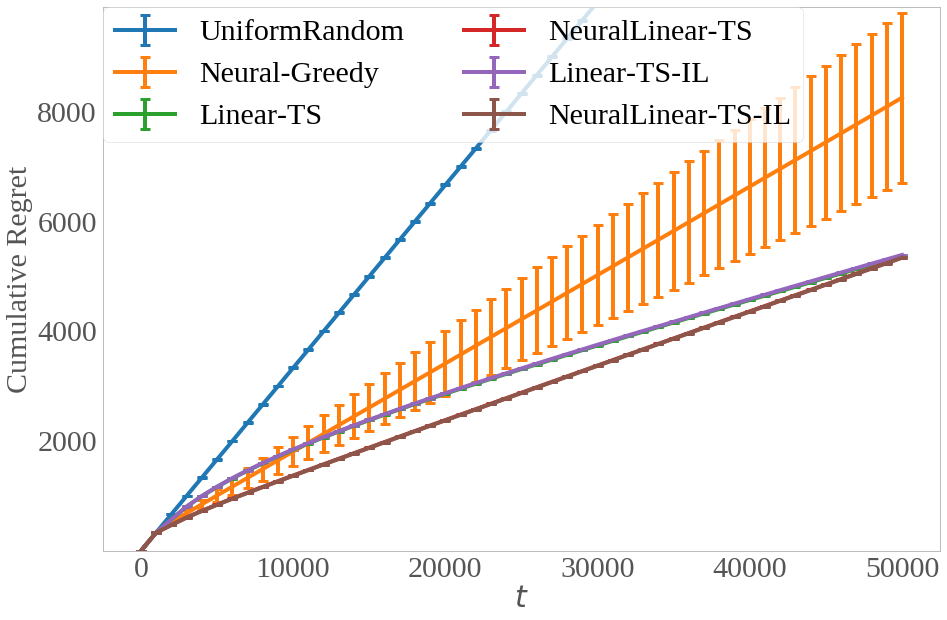
Figure 2: Cumulative regret on the Warfarin problem with 50 actions

Appendix G Time and Space Complexity

G.1 Complexity of Evaluated Methods

Table 2 shows the decision-making time complexity for the methods used in our empirical analysis. The time complexity is equivalent to the space complexity for all evaluated methods.

NeuralGreedy The time complexity of NeuralGreedy is the sum of matrix-vector multiplications involved in a forward pass.

Linear-TS The time complexity of Linear-TS is dominated by sampling from the joint posterior, which requires sampling from a multivariate normal with dimension $d$. To draw a sample from the joint posterior $P(\bm{\theta},\sigma)$ at decision time, we first sample the noise level $\tilde{\sigma}^{2}\sim\text{IG}(\alpha,\beta)$ and then sample $\tilde{\bm{\theta}}|\tilde{\sigma}^{2}\sim\mathcal{N}\big{(}\bm{\mu},\tilde{\sigma}^{2}\Lambda^{-1}\big{)}$. Rather than inverting the precision matrix $\tilde{\Sigma}=\tilde{\sigma}^{2}\Lambda^{-1}$, we compute root decomposition (e.g. a Cholesky decomposition) of the $d\times d$ precision matrix $\Lambda=LL^{T}$. The root decomposition can be computed once, with cost $O(d^{3})$, after an offline batch update and cached until the next batch update. Given $L^{T}$, we sample directly by computing $\tilde{\bm{\theta}}=\bm{\mu}+\bm{z}$, where

$$\frac{1}{\tilde{\sigma}}L^{T}\bm{z}=\bm{\zeta}$$ (21)

and $\bm{\zeta}\overset{\text{iid}}{\sim}\mathcal{N}(0,1)$. Since $L^{T}$ is upper triangular, Eqn. (21) can be solved using a backward substitution in quadratic time: $O(d^{2})$.

NeuralLinear-TS The time complexity of NeuralLinear-TS is the sum of a forward pass up to the last hidden layer and sampling from a multivariate normal with dimension $h_{M}$, where $h_{M}$ is the size of the last hidden layer.

IL The IL methods have the same time complexity as NeuralGreedy, ignoring the cost of sampling from multinomial with $k$ categories.

G.2 Complexity Using Embedded Actions

An alternative modeling approach for the non-imitation methods is to embed the action with the context as input to the reward model.

NeuralGreedy Using an embedded action, the time complexity for a forward pass up to the last layer is $O_{\text{last-layer}}=O\big{(}kd_{a}h_{1}+k\sum_{m=1}^{M-1}h_{m}h_{m+1}\big{)}$ because the input at decision time is a $k\times d_{a}$ matrix where the context is embedded with each of the $k$ actions and the each context-action vector has dimension $d_{a}$. The time complexity of computing the output layer remains $O(kh_{M})$. The space complexity remains linear in the number of parameters, but it also requires computing temporary intermediate tensors of size $k\times h_{m}$ for $m=1...M$: $O\big{(}d_{a}h_{1}+\sum_{m=1}^{M-1}h_{m}h_{m+1}+\sum_{m=1}^{M}kh_{m}\big{)}$.

Linear-TS Linear-TS with an embedded action only requires using a single sample of the parameters, which yields a complexity of to $O(d_{a}^{2}+kd_{a})$ for Linear-TS. The space complexity is also $O(d_{a}^{2}+kd_{a})$.

NeuralLinear-TS For NeuralLinear-TS the time complexity of computing the outputs given the last hidden layer is $O(h_{M}^{2}+kh_{M})$, since only a single sample of $h_{M}$ parameters is required for computed the reward for all actions. The space complexity for NeuralLinear-TS the sum the space complexities of NeuralGreedy and Linear-TS.

IL The cost of the IL methods would be unchanged.

We choose to empirically evaluate models without embedded actions because linear methods using embedded actions cannot model reward functions that involve non-linear interactions between the contexts and actions, whereas modeling each action independently allows for more flexibility. RiquelmeTuSn18 find that Thompson sampling using disjoint, exact linear bayesian regressions are a strong baseline in many applications. Furthermore, RiquelmeTuSn18 observe that it is important to model the noise levels independently for each action.

G.3 Complexity of Alternative Methods

Alternative Thompson sampling methods including mean-field approaches, the low-rank approximations of the covariance matrix, and bootstrapping can also decrease the cost of posterior sampling. Mean-field approaches can reduce time complexity of sampling parameters from the posterior from quadratic $O(n^{2})$ to linear $O(n)$ in the number of parameters $n$. However, assuming independence among parameters has been observed to result in worse performance in some settings (RiquelmeTuSn18). Low-rank approximations of the covariance matrix allow for sampling parameters in $O((n+1)\rho)$, where $\rho$ is the rank of the approximate covariance, but such methods have a space complexity of $O(\rho n)$ since they require storing $\rho$ copies of the parameters (zhang2018noisy; maddox2019swag). Bootstrapping also requires storing multiple copies of the parameters, so the space is $O(bn)$ where $b$ is the number of bootstrap replicates. However, bootstrapping simply requires a multinomial draw to select one set of bootstrapped parameters. All these methods require a forward pass using the sampled parameters, and the time complexity is the sum of the time complexities of sampling parameters and the forward pass.

Table 2: Decision-making time complexity and space complexity for each method (these are equivalent for all methods). For methods relying on fully-connected neural networks, the time complexity of a forward pass to the last hidden layer is $C_{\mbox{last-layer}}=dh_{1}+\sum_{m=1}^{M-1}h_{m}h_{m+1}$, where $d$ is the dimension of the context and $h_{m}$ is the number of units in hidden layer $m$.

Method	Time and Space Complexity
NeuralGreedy	$O(C_{\mbox{last-layer}})+O(kh_{M})$
Linear-TS	$O(kd^{2})$
NeuralLinear-TS	$O(C_{\mbox{last-layer}})+O\big{(}kh_{M}^{2})$
IL	$O(C_{\mbox{last-layer}})+O(kh_{M})$