Unveiling the architecture of a pulsar - binary black-hole triple system with pulsar arrival time analysis

Abstract

A large number of binary black holes (BBHs) with longer orbital periods are supposed to exist as progenitors of BBH mergers recently discovered with gravitational wave (GW) detectors. In our previous papers, we proposed to search for such BBHs in triple systems through the radial-velocity modulation of the tertiary orbiting star. If the tertiary is a pulsar, high precision and cadence observations of its arrival time enable an unambiguous characterization of the pulsar – BBH triples located at several kpc, which are inaccessible with the radial velocity of stars. The present paper shows that such inner BBHs can be identified through the short-term Rømer delay modulation, on the order of $10$ msec for our fiducial case, a triple consisting of $20~{}M_{\odot}$ BBH and $1.4~{}M_{\odot}$ pulsar with $P_{\mathrm{in}}=10$ days and $P_{\mathrm{out}}=100$ days. If the relativistic time delays are measured as well, one can determine basically all the orbital parameters of the triple. For instance, this method is applicable to inner BBHs of down to $\sim 1$ hr orbital periods if the orbital period of the tertiary pulsar is around several days. Inner BBHs with $\lesssim 1$ hr orbital period emit the GW detectable by future space-based GW missions including LISA, DECIGO, and BBO, and very short inner BBHs with sub-second orbital period can be even probed by the existing ground-based GW detectors. Therefore, our proposed methodology provides a complementary technique to search for inner BBHs in triples, if exist at all, in the near future.

1 Introduction

The presence of abundant binary black holes (BBHs) in the universe is now firmly established by their gravitational wave (GW) signals emitted at the final epoch of their merger event (e.g. Abbott et al., 2016, 2020). The formation channels of such BBHs are still controversial, but a variety of scenarios have been proposed, including the isolated binary evolution (e.g. Belczynski et al., 2002), the dynamical capture in stellar systems (e.g. Portegies Zwart & McMillan, 2000), and the interaction among primordial black holes (e.g. Sasaki et al., 2016).

Regardless of the details of those formation scenarios, the merging BBHs indicate that a significantly larger number of wide-orbit progenitor BBHs exist, losing their orbital energy before coalescence due to the gradual GW emission (e.g. Belczynski et al., 2016). Therefore, it is important to consider how to detect the population of such wide-separation BBHs that are supposed to be hidden even in our Galaxy.

Our previous papers (Hayashi et al., 2020; Hayashi & Suto, 2020, hereafter, Papers I and II) proposed a possible methodology to search for such progenitor BBHs in triple systems by precise radial velocity (RV) monitoring of a tertiary star orbiting an inner BBH. In the present paper, we extend the methodology for a triple system consisting of an inner BBH and a tertiary pulsar on the basis of the pulsar arrival time analysis.

The formation paths for such triples are highly uncertain, but there are several relevant theoretical studies (e.g. Toonen et al., 2016). Fragione et al. (2020), for instance, performed a series of systematic numerical simulations to find the demographics of stellar and compact-object triples assembled in dense star clusters. They found that binary-binary encounters efficiently form triples and that a cluster typically assembles hundreds of triples with an inner BBH (of which 70 - 90 % have a BH as tertiary) or an inner star-BH binary. Thus a triple of an inner BBH and a tertiary pulsar may be rare in the scenario.

On the other hand, more than 70 % of OBA-type stars and 50 % of FGK-type stars are known to be in multiples (Raghavan et al., 2010; Sana et al., 2012), and it is likely that yet unknown dynamical formation channel may account for pulsar - BBH triple systems.

Indeed, Ransom et al. (2014) discovered an interesting triple system with the pulsar timing, which consists of an inner binary of a $1.4~{}M_{\odot}$ millisecond pulsar (PSR J0337+1715) and $0.2~{}M_{\odot}$ white dwarf, and a tertiary white dwarf of $0.4~{}M_{\odot}$. Furthermore, the triple has near-coplanar and circular orbits; the mutual inclination $i_{\mathrm{mut}}$, inner eccentricity $e_{\mathrm{in}}$, and outer eccentricity $e_{\mathrm{out}}$ are $1.20\times 10^{-2}~{}\mathrm{deg}$, $6.9178\times 10^{-4}$, and $3.53561955\times 10^{-2}$, respectively.

While the presence of triples consisting of inner BBH and a tertiary pulsar is highly uncertain, and their fraction is expected to be smaller than star - BBH triples, the tertiary pulsar, if exists, is an ideal probe of the architecture of an otherwise unseen inner BBH of the triple system. The identification of an inner BBH from the precise radial-velocity of the tertiary star is possible only when the triple is located very close to us, typically much less than $\sim 1$ kpc. In contrast, the pulsar timing method is feasible for much more distant triples, even several kpc away. Thus the two methodologies may be regarded as complementary.

In this paper, we consider a pulsar orbiting an inner BBH, and show the signature and its amplitude of inner BBH hidden in the pulsar time of arrival (the Rømer delay). Furthermore, we point out that the other general relativistic effects, the Shapiro and Einstein delays, due to the inner BBH, significantly improves the understanding of the architecture of the triple system.

The rest of the paper is organized as follows. In section 2, we first introduce the overview of the time-delay effects in a triple. We additionally compare the amplitude of each effect using the analytic approximation formula for a coplanar and near-circular triple. Then, we discuss how we can recover the orbital information of a triple, such as masses and orbital separation, from detection of each effect in principle. In section 3, we show the time-delay curves of each effect for three models using the analytic expressions of time-delay effects. In section 4, we put rough constraints on the currently known double neutron-star binaries from root mean squares of the observational time residuals. In addition, we discuss the possibility of our methodology as a complementary technique to the future direct observation of low-frequency GWs with space-based GW detectors including LISA, DECIGO, and BBO. Finally, we make a conclusion in section 5. In the Appendix, we briefly discuss the modulation on the Keplerian motion induced by the inner-binary perturbation using the analytical formulation of perturbation.

2 Method

2.1 Triple configuration

Figure 1 depicts the schematic configuration of a hierarchical triple system considered in the present paper. The inner binary comprises two BHs of masses $m_{1}$ and $m_{2}$, and is orbited by a tertiary pulsar of mass $m_{3}$. While we assume the inner BBH, the discussion below is equally applicable to other compact objects like white dwarfs (WDs) and neutron stars (NSs).

The orbits in the triple system are divided into an inner and outer orbits in terms of the Jacobi coordinates, and each orbit is characterized by the semi-major axis $a_{j}$, the eccentricity $e_{j}$, and the argument of pericenter $\omega_{j}$, where the index $j=\{\mathrm{in},\mathrm{out}\}$ refers to the inner and outer orbits, respectively. The orientation of each orbit is specified by two angles relative to the reference frame; the inclination $I_{j}$ (the angle between the normal vector of the orbit and $z$-axis) and the longitude of ascending node $\Omega_{j}$ measured from $x$-axis.

The mutual inclination between the inner and outer orbits is denoted by $i_{\mathrm{mut}}$, and the orbital period and the corresponding mean motion for each orbit are defined as $P_{j}$ and $\nu_{j}(=2\pi/P_{j})$. Throughout the present analysis, we consider a hierarchical triple system that satisfies $P_{\mathrm{in}}\ll P_{\mathrm{out}}$. For definiteness, we assume that the distant observer is located in the negative $z$-axis.

Following Paper II, we assume a fiducial set of parameters, $P_{\mathrm{in}}=10$ days, $P_{\mathrm{out}}=100$ days, and $m_{1}=m_{2}=10~{}M_{\odot}$, which will be used in evaluating characteristic amplitudes of the time delays.

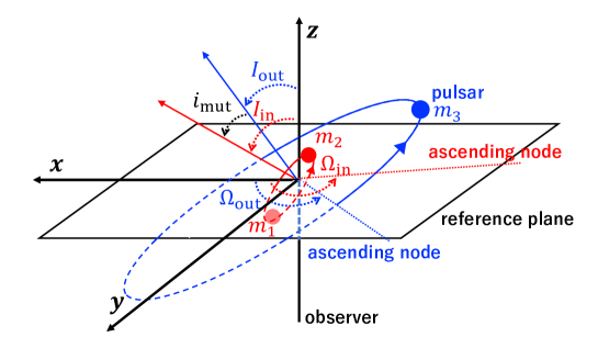
Figure 1: Orbital configuration of a triple system consisting of an inner unseen binary and a tertiary millisecond pulsar. The origin of the reference frame is set to be the barycenter of the inner binary, instead of the triple.

2.2 Pulsar arrival time delays

The architecture of the triple system is encoded by the motion of the tertiary object orbiting the unseen inner binary. If the tertiary is a visible star, its radial velocity carries the key information (Papers I and II). If the tertiary is a pulsar, its arrival time variation has almost identical information of its radial velocity, but with much higher precision. Furthermore, general relativistic effects provide additional and complementary information on the parameters of the triple system.

The arrival time of the pulsar is modulated due to the periodic change of the position of the pulsar. For a pulsar binary system, there are three well-known effects including the Rømer delay $\Delta_{\mathrm{R}}(t)$, the Einstein delay $\Delta_{\mathrm{E}}(t)$, and the Shapiro delay $\Delta_{\mathrm{S}}(t)$. In the case of the hierarchical triple system, the main contribution to those three terms comes from the approximate binary motion of the pulsar relative to the barycenter of the inner binary of mass $m_{12}\equiv m_{1}+m_{2}$, whose explicit expressions(e.g Backer & Hellings, 1986; Edwards et al., 2006) are given in this subsection. More importantly, the inner binary produces an additional modulation to the tertiary motion of a period approximately $P_{\mathrm{in}}/2$. Consequently, the Rømer delay is given by $\Delta_{\mathrm{R,Kep}}(t)$ and $\Delta_{\mathrm{R,BBH}}(t)$ that can be distinguished from their different frequencies. Indeed the inner binary information is imprinted in $\Delta_{\mathrm{R,BBH}}(t)$ as we will see below.

2.2.1 The Rømer delay due to the Keplerian motion of the tertiary pulsar

The Rømer delay is caused by the change of the distance of the pulsar relative to the observer. To the lowest order, the pulsar moves along a Keplerian orbit around the barycenter of the triple system. The corresponding Rømer delay is written in terms of the eccentric anomaly of the outer orbit, $E_{\mathrm{out}}=E_{\mathrm{out}}(t)$, as

$$\Delta_{\mathrm{R,Kep}}(t)=x[\sin{\omega_{\mathrm{out}}}(\cos{E_{\mathrm{out}}}-e_{\mathrm{out}})+\sqrt{1-e_{\mathrm{out}}^{2}}\cos{\omega_{\mathrm{out}}}\sin{E_{\mathrm{out}}}]$$ (1)

The eccentric anomaly is expressed implicitly as function of time through Kepler’s equation:

$$2\pi t=P_{\mathrm{out}}(E_{\mathrm{out}}-e_{\mathrm{out}}\sin E_{\mathrm{out}}).$$ (2)

Note that we can only observe the difference of the time delay, and can choose arbitrarily the zero point of the overall time delays.

Since the semi-major axis of the outer orbit, $a_{\mathrm{out}}$, is defined with respect to the center of mass of the inner binary, that of the pulsar orbit with respect to the barycenter of the triple is given by $a_{\rm p}=(m_{12}/m_{123})a_{\mathrm{out}}$, where $m_{12}\equiv m_{1}+m_{2}$ and $m_{123}\equiv m_{1}+m_{2}+m_{3}$. Thus the amplitude of the Rømer delay for a distant observer at the negative $z$-direction (Fig.1) reduces to

$$x\equiv\frac{m_{12}}{m_{123}}\frac{a_{\mathrm{out}}\sin{I_{\mathrm{out}}}}{c}\approx 570~{}\mathrm{sec}\left(\frac{m_{12}}{m_{123}}\right)\left(\frac{m_{123}}{20~{}M_{\odot}}\right)^{1/3}\left(\frac{P_{\mathrm{out}}}{100~{}\mathrm{days}}\right)^{2/3}\sin{I_{\mathrm{out}}}.$$ (3)

2.2.2 The Einstein delay and the Shapiro delay

In addition to the Rømer delay, there are two important general relativistic effects that carries the information of the triple system; the Einstein delay and the Shapiro delay.

The Einstein delay is caused by the difference between the proper time of the pulse emission and the coordinate time of the barycenter of the binary under the gravitational field, and is explicitly expressed as

$$\Delta_{\mathrm{E}}(t)=\gamma_{\mathrm{E}}\sin{E_{\mathrm{out}}},$$ (4)

where the amplitude is given by

$$\gamma_{\mathrm{E}} \equiv \left(\frac{\mathcal{G}}{c^{3}}\right)^{2/3}\left(\frac{P_{\mathrm{out}}}{2\pi}\right)^{1/3}e_{\mathrm{out}}\frac{m_{12}(m_{3}+2m_{12})}{m_{123}^{4/3}}$$ (5)

$$\approx 2.4~{}\mathrm{msec}\left(\frac{P_{\mathrm{out}}}{100~{}\mathrm{days}}\right)^{1/3}\left(\frac{m_{12}}{20~{}M_{\odot}}\right)\left(\frac{m_{123}}{20~{}M_{\odot}}\right)^{-1/3}\left(1+\frac{m_{12}}{m_{123}}\right)\left(\frac{e_{\mathrm{out}}}{0.01}\right)$$ (6)

with $\mathcal{G}$ being the gravitational constant.

The Shapiro delay is the time delay during the passage of the photon due to the gravitational space-time curvature of the companion, and is given by

$$\Delta_{\mathrm{S}}(t) = -2r\ln\left[1-e_{\mathrm{out}}\cos{E_{\mathrm{out}}}\right.$$ (8)

$$\qquad\qquad\qquad\left.-s\left(\sin{\omega_{\mathrm{out}}}(\cos{E_{\mathrm{out}}}-e_{\mathrm{out}})+\sqrt{1-e_{\mathrm{out}}^{2}}\cos{\omega_{\mathrm{out}}}\sin{E_{\mathrm{out}}}\right)\right],$$

where $r$ and $s$ are the major observables and usually referred to as “range” and “shape” parameters(e.g Backer & Hellings, 1986; Edwards et al., 2006):

$$r \equiv \frac{\mathcal{G}m_{12}}{c^{3}}\approx 98~{}\mathrm{\mu sec}\left(\frac{m_{12}}{20~{}M_{\odot}}\right),$$ (9)

$$s \equiv \sin{I_{\mathrm{out}}}.$$ (10)

As equations (4) and (8) indicate, $\Delta_{\mathrm{S}}\ll\Delta_{\mathrm{E}}$ except for for a nearly circular and edge-on system ($e_{\mathrm{out}}\approx 0$ and $s\approx 1$). A notable example is a binary pulsar system PSR J1614-2230 with $e_{\mathrm{out}}=1.30\times 10^{-6}$ and $I_{\mathrm{out}}=89.17$ deg, which reveals the mass of the pulsar is as massive as $1.97~{}M_{\odot}$ via the analysis of the Shapiro delay (Demorest et al., 2010).

In principle, the Shapiro delays for both inner and outer orbits may be separately detected, especially for nearly edge-on coplanar systems ($I_{\mathrm{out}}\approx I_{\mathrm{in}}\approx\pi/2$). In this case, the Shapiro delays alone directly reveal the existence of the inner binary and their individual masses $m_{1}$ and $m_{2}$. In what follows, however, we conservatively consider only the Shapiro delay for the outer orbit, assuming the inner binary as a single object of mass $m_{12}$.

2.2.3 The Rømer delay due to the inner binary motion

The orbital motion of the inner BBH perturbs the Keplerian motion of the tertiary. Papers I and II proposed to detect the induced radial velocity modulation of the tertiary star to search for a possible inner BBH in the triple systems. In the case of a coplanar and near-circular hierarchical triple, the corresponding radial velocity variation up to the quadrupole order of the BBH potential is approximately given by (Morais & Correia, 2008, see also paper I and II)

$$\dot{z}_{\mathrm{BBH}}(t)=\frac{15}{16}K_{\rm\scriptscriptstyle BBH}\sin{I_{\mathrm{out}}}\cos(\nu_{-3}t+\theta_{0,-3})+\frac{3}{16}K_{\rm\scriptscriptstyle BBH}\sin{I_{\mathrm{out}}}\cos(\nu_{-1}t+\theta_{0,-1}),$$ (11)

where the characteristic velocity amplitude is

$$K_{\rm\scriptscriptstyle BBH}\equiv\frac{m_{1}m_{2}}{m_{12}^{2}}\sqrt{\frac{m_{123}}{m_{12}}}\left(\frac{a_{\mathrm{in}}}{a_{\mathrm{out}}}\right)^{7/2}\times\left[\frac{m_{12}}{m_{123}}a_{\mathrm{out}}\nu_{\mathrm{out}}\right]$$ (12)

with the term inside the square bracket corresponding to the velocity of the circular Keplerian motion, and the frequencies of the two modes are

$$\nu_{-3} \equiv 2\nu_{\mathrm{in}}-3\nu_{\mathrm{out}}$$ (13)

$$\nu_{-1} \equiv 2\nu_{\mathrm{in}}-\nu_{\mathrm{out}},$$ (14)

with $\theta_{0,-3}$ and $\theta_{0,-1}$ being the initial phases. For the hierarchical triples ($\nu_{\mathrm{in}}\gg\nu_{\mathrm{out}}$), $\nu_{-3}\approx\nu_{-1}\approx 2\nu_{\mathrm{in}}=4\pi/P_{\mathrm{in}}$. Thus the high-cadence radial velocity observation is required to break the degeneracy of the two modes.

Equation (11) is directly translated to the short-term Rømer delay:

$$\Delta_{\mathrm{R,BBH}}(t)\equiv\frac{z_{\rm\scriptscriptstyle BBH}(t)}{c} = \frac{15}{16}\frac{K_{\rm\scriptscriptstyle BBH}P_{\mathrm{in}}}{4\pi c}\left(\frac{2\nu_{\mathrm{in}}}{\nu_{-3}}\right)\sin{I_{\mathrm{out}}}\sin(\nu_{-3}t+\theta_{0,-3})$$ (15)

$$+ \frac{3}{16}\frac{K_{\rm\scriptscriptstyle BBH}P_{\mathrm{in}}}{4\pi c}\left(\frac{2\nu_{\mathrm{in}}}{\nu_{-1}}\right)\sin{I_{\mathrm{out}}}\sin(\nu_{-1}t+\theta_{0,-1}).$$ (16)

The characteristic amplitude of equation (15) is

$$\frac{K_{\rm\scriptscriptstyle BBH}P_{\mathrm{in}}}{4\pi c}\sin{I_{\mathrm{out}}} = \frac{1}{2}\frac{m_{1}m_{2}}{m_{12}^{2}}\left(\frac{m_{12}}{m_{123}}\right)^{2/3}\left(\frac{P_{\mathrm{in}}}{P_{\mathrm{out}}}\right)^{7/3}x$$ (17)

$$\approx 23~{}\mathrm{msec}\left(\frac{K_{\rm\scriptscriptstyle BBH}}{100~{}\mathrm{m/s}}\right)\left(\frac{P_{\mathrm{in}}}{10~{}\mathrm{days}}\right)\sin{I_{\mathrm{out}}},$$ (18)

implying that the inner BBH motion is much larger than the general relativistic terms in general. Furthermore, the high-cadence monitoring of the pulsar timing can break the degeneracy between the $\nu_{-3}$ and $\nu_{-1}$ modes more easily than in the radial velocity measurements of main-sequence stars.

Figures 2 and 3 show the contour plots of the characteristic amplitude of the Rømer delay induced by the inner BBH, equation (17), for the case of a coplanar and near-circular triple with our fiducial set of parameters. Figure 2 is plotted on the $m_{2}/m_{1}$ and $P_{\mathrm{in}}$ plane for $P_{\mathrm{out}}=100$ days, while Figure 3 is plotted on the $P_{\mathrm{out}}$ and $P_{\mathrm{in}}$ plane for $m_{1}=m_{2}=10~{}M_{\odot}$. Since typical amplitudes of the pulsar timing noise is less than $O(100)~{}\mu$sec (see, e.g., Table 2), the Rømer delay induced by the inner BBH for our fiducial triple may be easily detected as long as precise and high-cadence pulsar-timing data are available.

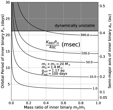
Figure 2: Characteristic amplitude of the Rømer delay induced by the inner BBH as a function of the inner-binary orbital period ($P_{\mathrm{in}}$) and mass ratio ($m_{2}/m_{1}$). We assume a coplanar and circular triple system with the following parameters; the total mass of the inner BBH $m_{1}+m_{2}=20~{}M_{\odot}$, the tertiary pulsar mass $m_{3}=1.4~{}M_{\odot}$, the outer orbital period $P_{\mathrm{out}}=100$ days corresponding to the outer semi-major axis of $a_{\mathrm{out}}=1.17$ au). The upper shaded region is dynamically unstable from the criterion by Mardling & Aarseth (1999).

Figure 4 compares the characteristic amplitudes of the four time delays as a function of the mass $m_{12}$ and the outer orbital period $P_{\mathrm{out}}$ for an equal-mass inner binary with the tertiary mass of $m_{3}=1.4~{}M_{\odot}$. The upper-left, upper-right, lower-left, and lower-right panels show the Rømer delay of the outer Keplerian motion, the Einstein delay, the Shapiro delay, and the Rømer delay induced by the inner binary perturbation, respectively. The solid and dotted black lines in the lower-right panel show the contour curves for the cases that $P_{\mathrm{in}}=P_{\mathrm{out}}/10$, $P_{\mathrm{out}}/50$, respectively. Note that the amplitude of the Shapiro delay is very sensitive to the shape parameter $s=\sin I_{\mathrm{out}}$ as indicated by equation (8). Therefore, the amplitude of the range parameter $r$ plotted in Figure 4 should be regarded as a very rough estimate of the expected Shapiro delay.

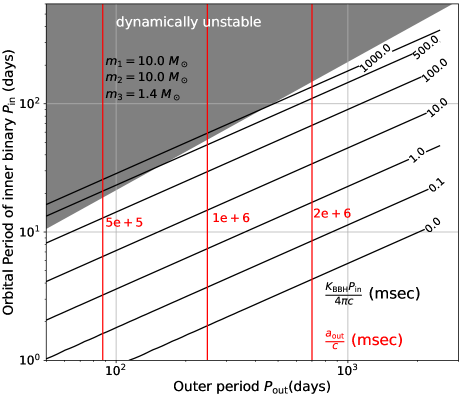
Figure 3: Characteristic amplitude of the Rømer delay induced by the equal-mass inner-BBH as a function of the inner and outer orbital periods. We assume the same parameters for the triple system as in Figure 2 except that $m_{1}=m_{2}=10~{}M_{\odot}$ and $P_{\mathrm{out}}$ is a variable. For reference, the Rømer delay amplitude due to the tertiary Keplerian motion is plotted in red lines.

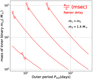
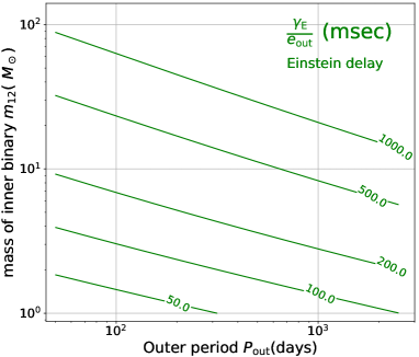
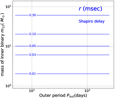
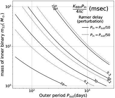
Figure 4: Characteristic amplitudes of each time-delay effect as a function of the outer orbital period $P_{\mathrm{out}}$ and total mass of the inner BBH $m_{12}$. The upper-left, upper-right, lower-left, and lower-right panels plot the Rømer delay of the Keplerian motion, the Einstein delay, the Shapiro delay, and the Rømer delay by the inner binary perturbation, respectively. The solid and dotted black lines in the lower-right panel show the Rømer time delay induced by the inner binary with $P_{\mathrm{in}}$ being $P_{\mathrm{out}}/10$ and $P_{\mathrm{out}}/50$, respectively. Note that the amplitude of the Shapiro delay is sensitive to the inclination $I_{\mathrm{out}}$, or equivalently to the shape parameter $s=\sin I_{\mathrm{out}}$ (see Figure 6, for example). Thus, the range parameter $r$ is just a very crude estimate of the amplitude.

2.3 Constraints on parameters from individual time delay data

There are 13 parameters (three masses and ten orbital parameters except for the initial positions of the bodies) in total that specify the triple system, and the four time delays discussed in the above subsection put different constraints on those parameters. We show those constraints separately for each time delay measurement in this subsection, and consider how their combination determines the properties of the inner BBH in the next subsection. The procedure to estimate orbital parameters for the triple system with a tertiary pulsar is summarized in Figure 5

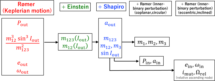
Figure 5: Summary of orbital parameters that are estimated from the pulsar arrival timing analysis.

Consider first the Rømer time delay of the Keplerian motion. Strictly speaking, all the orbital parameters in equation (1) are not constant except for the two-body system. For the hierarchical triple system that we consider here, those parameters typically vary over the Kozai-Lidov timescale:

$$\tau_{\rm KL}\equiv\frac{m_{12}}{m_{3}}\frac{P_{\mathrm{out}}}{P_{\mathrm{in}}}P_{\mathrm{out}}.$$ (19)

Throughout the present paper, we assume that the duration of the pulsar arrival time data is much less than $\tau_{\rm KL}$, and that the orbital parameters are approximately constant. Even if it is not the case, however, the methodology that we propose here remains the same, but it requires numerical integration of the three-body dynamics so as to properly account for the time-dependence of the orbital parameters.

Under the approximation, fitting equation (1) to the series of the pulsar arrival time data determines the values of $e_{\mathrm{out}}$, $\omega_{\mathrm{out}}$, and $P_{\mathrm{out}}$, in addition to the overall amplitude $x=m_{12}a_{\mathrm{out}}\sin{I_{\mathrm{out}}}/(cm_{123})$. Combining Kepler’s third law $a_{\mathrm{out}}^{3}/P_{\mathrm{out}}^{2}=(\mathcal{G}m_{123}/4\pi^{2})$, one obtains the following relation:

$$\frac{m_{12}^{3}\sin^{3}{I_{\mathrm{out}}}}{(m_{12}+m_{3})^{2}}=(cx)^{3}\mathcal{G}^{-1}\left(\frac{2\pi}{P_{\mathrm{out}}}\right)^{2}.$$ (20)

Indeed, this is the binary mass function expressed in the observables from the Rømer delay measurement.

Second, the Einstein delay, equation (4), yields $e_{\mathrm{out}}$ and $P_{\mathrm{out}}$ through equation (2), and $\gamma_{\mathrm{E}}$. From the three parameters, one obtains

$$\frac{m_{12}(m_{123}+m_{12})}{m_{123}^{4/3}}=\frac{\gamma_{\mathrm{E}}}{e_{\mathrm{out}}}\left(\frac{2\pi}{P_{\mathrm{out}}}\right)^{1/3}\left(\frac{\mathcal{G}}{c^{3}}\right)^{-2/3}.$$ (21)

Equation (21) is another useful constraint on $m_{123}$ and $m_{12}$ that is independent of $I_{\mathrm{out}}$ unlike equation (20) from the Rømer delay.

Third, the Shapiro delay, equation (8), is particularly useful to determine $I_{\mathrm{out}}(=\sin^{-1}s)$, in addition to $e_{\mathrm{out}}$, $P_{\mathrm{out}}$, and $r$. Also the range parameter $r$, equation (9), is directly related to the total mass of the inner BBH binary:

$$m_{12}=r\left(\frac{\mathcal{G}}{c^{3}}\right)^{-1}.$$ (22)

Thus, the detection of the Shapiro delay plays a crucial and complementary role in breaking the degeneracy of the parameter estimation, especially for systems with $\sin I_{\mathrm{out}}\approx 1$. We also emphasize that the individual detection of the Shapiro delays for both components of the inner orbit would clearly break the degeneracy of the triple architecture of the system. This is likely to be the case if the triple is a nearly coplanar and edge-on system, and one can separately estimate the mass of the inner binary $m_{1}$ and $m_{2}$ from the Shapiro delays alone.

So far the above observables are mainly for the outer orbital parameters, and the Rømer delay by inner binary motion is the key observable to unveil the properties of the inner BBH. In order to show an specific example, we consider a coplanar near-circular triple expressed in equation (15). Fitting equation (15) to the pulsar arrival timing data yields

$$P_{\mathrm{in}}=\frac{8\pi}{3\nu_{-1}-\nu_{-3}}$$ (23)

and

$$\frac{m_{1}m_{2}}{m_{12}^{2}}\left(\frac{a_{\mathrm{in}}}{a_{\mathrm{out}}}\right)^{7/2}\sqrt{\frac{m_{123}}{m_{12}}}=\frac{K_{\rm\scriptscriptstyle BBH}}{cx}\left(\frac{P_{\mathrm{out}}}{2\pi}\right).$$ (24)

2.4 Inner-binary parameters from joint analysis of time delays

In this section, we show how the orbital parameters of an unseen inner BBH can be recovered from the joint analysis of the pulsar arrival time.

As discussed in the previous subsection, the dominant contribution comes from the Rømer delay from the Keplerian motion of the outer orbit, which derives $e_{\mathrm{out}}$, $P_{\mathrm{out}}$, $\omega_{\mathrm{out}}$, and $x$. If the Einstein delay is detected as well, the total mass of the system $m_{123}$ and inner binary mass $m_{12}$ are written in terms of the observables and $\sin I_{\mathrm{out}}$ from combining equations (20) and (21):

$$m_{123}=\left(\frac{\mathcal{G}}{c^{3}}\right)^{-1}\frac{1}{x^{3}}\left(\frac{P_{\mathrm{out}}}{2\pi}\right)\left[\frac{\gamma_{\mathrm{E}}}{e_{\mathrm{out}}}-\frac{x^{2}}{\sin^{2}{I_{\mathrm{out}}}}\left(\frac{P_{\mathrm{out}}}{2\pi}\right)^{-1}\right]^{3}$$ (25)

and

$$m_{12}=\left(\frac{\mathcal{G}}{c^{3}}\right)^{-1}\frac{1}{x\sin{I_{\mathrm{out}}}}\left[\frac{\gamma_{\mathrm{E}}}{e_{\mathrm{out}}}-\frac{x^{2}}{\sin^{2}{I_{\mathrm{out}}}}\left(\frac{P_{\mathrm{out}}}{2\pi}\right)^{-1}\right]^{2}.$$ (26)

In addition, if the Shapiro delay is detected, $\sin I_{\mathrm{out}}$ and $m_{12}$ are derived directly from the range and shape parameters $r$ and $s$, respectively. Thus equation (26) provides a consistency relation among observables:

$$r=\frac{1}{sx}\left[\frac{\gamma_{\mathrm{E}}}{e_{\mathrm{out}}}-\frac{x^{2}}{s^{2}}\left(\frac{P_{\mathrm{out}}}{2\pi}\right)^{-1}\right]^{2}.$$ (27)

Using equation (27), equation (25) is rewritten in terms of the observables alone:

$$m_{123}=\left(\frac{\mathcal{G}}{c^{3}}\right)^{-1}\left(\frac{sr}{x}\right)^{3/2}\left(\frac{P_{\mathrm{out}}}{2\pi}\right).$$ (28)

Therefore, the mass of the tertiary can be estimated as

$$m_{3}=m_{123}-m_{12}=\left(\frac{\mathcal{G}}{c^{3}}\right)^{-1}\left[\left(\frac{sr}{x}\right)^{3/2}\left(\frac{P_{\mathrm{out}}}{2\pi}\right)-r\right].$$ (29)

Since the mass of a neutron star is $(1-2)~{}M_{\sun}$, equation (29) may be also used as a consistency check of the analysis. Similarly the semi-major axis of the outer orbit can be written as

$$a_{\mathrm{out}}=c\left(\frac{P_{\mathrm{out}}}{2\pi}\right)\left(\frac{sr}{x}\right)^{1/2}.$$ (30)

Finally, the Rømer delay by the inner binary perturbation, if observed at all, elucidates the inner orbital parameters from the inner orbital period $P_{\mathrm{in}}$, and the velocity variation amplitude $K_{\rm\scriptscriptstyle BBH}$; see equation (15).

Specifically, each mass of inner binary components $m_{1,2}$ and the inner orbital semi-major axis $a_{\mathrm{in}}$ are written as follows:

$$a_{\mathrm{in}}=cr^{1/3}\left(\frac{P_{\mathrm{in}}}{2\pi}\right)^{2/3}$$ (31)

and

$$m_{1,2}=\left(\frac{\mathcal{G}}{c^{3}}\right)^{-1}\left(\frac{r}{2}\right)\left[1\pm\sqrt{1-\frac{4K_{\rm\scriptscriptstyle BBH}}{c}\left(\frac{2\pi r}{P_{\mathrm{in}}}\right)^{7/3}\left(\frac{P_{\mathrm{out}}}{2\pi}\right)^{4}(rx)^{-2}}\right].$$ (32)

Note that the above equations are written in terms of the observables from the Rømer delays of the Keplerian motion and inner binary perturbation, and the Shapiro delay, but without the Einstein delay measurement.

3 Effects of the eccentricity and inclination of the inner binary on the pulsar arrival time

While the analytic discussion presented in the previous section assumes a coplanar near-circular triple, the procedure of the triple parameter extraction is the same except that the evolution of the triple system needs to be computed numerically in general. We demonstrate the eccentricity and inclination effects on the pulsar arrival time separately in this section using the approximate analytic formulae by Morais & Correia (2011).

For that purpose, we consider three models listed in Table 1; a coplanar circular triple (model CC), a coplanar eccentric triple (model CE), and an inclined circular triple (model IC).

Figure 6 plots the time-delay curves for the three models. The upper-left, upper-right, and lower-left panels show the Rømer, Einstein, and Shapiro delays, respectively, due to the outer Keplerian motion of a tertiary pulsar of period $P_{\mathrm{out}}$. Strictly speaking, the outer orbit is perturbed by the inner-binary motion as well, but we neglect such small perturbations in those three panels for simplicity. Therefore these three time-delays are computed from equations (1), (4), and (8). The perturbed outer Keplerian motion has been extensively discussed in Paper II, and the result (with some improvement relative to Paper II) is given in Appendix.

Thus the unseen inner-binary parameters are encoded only in the Rømer delay modulation plotted in the lower-right panel of Figure 6, which is computed from equation (15) for model CC, and the analytic perturbative formulae derived in Morais & Correia (2011) for models CE and IC.

The upper-left panel of Figure 6 indicates that the outer eccentricity $e_{\mathrm{out}}$ distorts the sinusoidal curve of the Rømer delay to some extent, according to equation (1). Note that the constant offset in the figure is not relevant, and the eccentricity changes the shape of the delay. On the other hand, the Einstein delay (upper-right panel) is very sensitive to $e_{\mathrm{out}}$ since equation (4) is proportional to $e_{\mathrm{out}}$.

Since the Shapiro delay is especially sensitive to the inclination of the outer orbit relative to the observer, the lower-left panel plots three different cases for $I_{\mathrm{out}}$; nearly edge-on ($85$ deg), moderately inclined ($60$ deg), and nearly face-on ($30$ deg) for each model. While the amplitude of the Shapiro delay is smaller than the Rømer delay and the Einstein delay for an eccentric orbit, it provides a unique constraint on $I_{\mathrm{out}}$, especially for an inclined outer orbit, that is useful to break the parameter degeneracy as emphasized in the previous section.

Table 1: Models of non-circular/non-coplanar triples

	$e_{\mathrm{in}}$	$e_{\mathrm{out}}$	$i_{\mathrm{mut}}$ (deg)
CC (coplanar circular)	0.0	0.01	0.0
CE (coplanar eccentric)	0.2	0.3	0.0
IC (inclined circular)	0.0	0.01	45

Note. — We adopt the same values for the other triple parameters: $m_{1}=$ $m_{2}=10~{}M_{\odot}$, $m_{3}=1.4~{}M_{\odot}$. $P_{\mathrm{in}}=10$ days, $P_{\mathrm{out}}=100$ days. The angles are $\omega_{\mathrm{in}}=30$ deg, $\omega_{\mathrm{out}}=60$ deg, $\Omega_{\mathrm{in}}=\Omega_{\mathrm{out}}=0$ deg, and the initial true anomalies $f_{\mathrm{in}}=120$ deg and $f_{\mathrm{out}}=0$ deg.

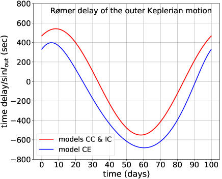
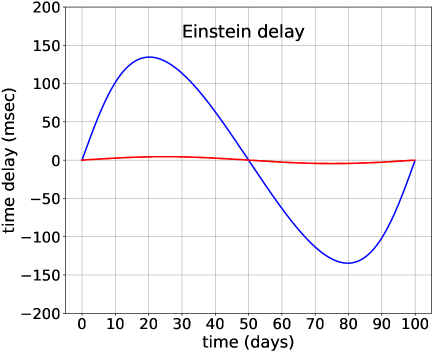
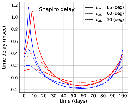
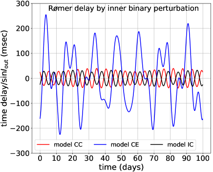
Figure 6: The time-delay curves of the Rømer delay by the outer Keplerian motion (upper-left), the Einstein delay (upper-right), the Shapiro delay (lower-left), and the Rømer delay induced by the inner binary perturbation (lower-right) for the three models listed in Table 1, respectively. The Rømer delay by the inner-binary perturbation only shows the time-delay modes associated with the inner-binary frequency $\nu_{\mathrm{in}}$.

Finally the lower-right panel, the Rømer delay due to the inner-binary perturbation, exhibits a clear shorter-term modulation (of period $\approx P_{\mathrm{in}}/2$) periodicity, whose shape is also sensitive to the inner eccentricity and inclination. Therefore, the detection of such short-term periodic features in the time delay component is a promising probe of the possible inner BBH of the unseen companion of the pulsar.

4 Application to the existing binary neutron stars as a proof of concept to constrain an unseen inner binary

Our methodology proposed in the present paper requires target pulsar binary systems with an unseen massive companion. The detection of the Rømer delay modulation much shorter than the pulsar’s Keplerian orbital period is an unambiguous proof that the unseen companion is indeed a binary, instead of a single object. While no interesting candidate is known for which our methodology can be applied, we attempt to put constraints on a possible inner binary for a companion of existing double neutron star (DNS) binaries through available pulsar arrival timing data.

4.1 Pulsar arrival timing constraints

Table 2 summarizes the current list of known DNS systems with their orbital parameters derived from the pulsar timing observations. Since they are interpreted as a binary system, $m_{12}$ and $m_{123}$ in Table 2 correspond to the companion mass of the pulsar, and the total mass of the system, respectively. Since both $m_{12}$ and $m_{123}-m_{12}$ are in the typical mass range of neutron stars, it is very unlikely that those companions are binaries of white dwarfs or black holes. Nevertheless, the null detection of the Rømer delay modulation due to the inner binary motion within the root mean square of the residuals $\sigma_{\mathrm{rms}}$ (the eighth column of Table 2) can put observational constraints on the inner binary.

In the practical analysis of the pulsar timing, however, the signals from a triple may be degenerated with other parameters on a pulsar, which may obscure the interpretation or even the presence of the inner BBH if one relies on the standard pipeline that neglects the possible triple effects. Therefore, an improved analysis taking account of such effects is required to constrain the system in a more quantitative and reliable fashion. This is beyond the scope of the present paper, but we are working on this problem and plan to show the result elsewhere (Kumamoto, Hayashi, Takahashi, and Suto, in preparation).

Because this is intended to be a merely proof-of-concept analysis, we simply constrain those systems by assuming a coplanar near-circular inner binary. Then using equation (15), the inner orbital period $P_{\mathrm{in}}$ is constrained as

$$\frac{K_{\rm\scriptscriptstyle BBH}P_{\mathrm{in}}}{4\pi c}\sin{I_{\mathrm{out}}} = \frac{1}{2}\frac{m_{1}m_{2}}{m_{12}^{2}}\left(\frac{m_{12}}{m_{123}}\right)^{2/3}\left(\frac{P_{\mathrm{in}}}{P_{\mathrm{out}}}\right)^{7/3}x<\sigma_{\mathrm{rms}}.$$ (33)

If we further assume an equal-mass inner binary ($m_{1}=m_{2}$), the above inequality reduces to

$$\frac{P_{\mathrm{in}}}{P_{\mathrm{out}}}<\left(\frac{8\sigma_{\mathrm{rms}}}{x}\right)^{3/7}\left(\frac{m_{123}}{m_{12}}\right)^{2/7}\approx 0.009\left(\frac{\sigma_{\mathrm{rms}}}{10~{}\mu\mathrm{sec}}\right)^{3/7}\left(\frac{x}{5~{}\mathrm{sec}}\right)^{-3/7}\left(\frac{m_{123}}{m_{12}}\right)^{2/7}.$$ (34)

The second column of Table 3 corresponds to the above upper limit on $P_{\mathrm{in}}$ for a hypothetical equal-mass inner binary in a coplanar near-circular triple. Those upper limits on $P_{\mathrm{in}}$ are typically less than an hour, implying the future pulsar timing observation for pulsar – massive BH binary candidates, if discovered in future, would strongly constrain the unseen inner binary in a similar fashion.

Table 2: List of known double neutron star systems

System	$P_{\mathrm{pulse}}$ (msec)	$P_{\mathrm{out}}$ (days)	$e_{\mathrm{out}}$	$x$ (sec)	$m_{123}~{}(M_{\odot})$	$m_{12}~{}(M_{\odot})$	$\sigma_{\mathrm{rms}}~{}(\mathrm{\mu sec})$	$T_{\mathrm{obs}}$ (yrs)	Ref.
J0453+1559	45.8	4.072	0.113	14.467	2.733	1.174	3.88	2.4	(1)
J0509+3801	76.5	0.380	0.586	2.051	2.80	1.46	102.36	3.1	(2)
J0737-3039A	22.7	0.102	0.088	1.415	2.587	1.249	54	2.7	(3)
J0737-3039B	2773	0.102	0.088	1.516	2.587	1.249	2169	2.7	(3)
J1411+2551	62.5	2.616	0.170	9.205	2.538	$>0.92$	32.77	2.4	(4)
J1518+4904	40.9	8.634	0.249	20.044	2.718	$>1.55$	6.05	13	(5)
B1534+12	37.9	0.421	0.274	3.729	2.679	1.346	4.57	22	(6)
J1753-2240	95.1	13.638	0.304	18.115	–	$>0.4875$	400	1.8	(7)
J1756-2251	28.5	0.320	0.181	2.756	2.571	1.230	19.3	9.6	(8)
J1757-1854	21.5	0.184	0.606	2.238	2.733	1.3946	36	1.6	(9)
J1811-1736	104.2	18.779	0.828	34.783	2.57	$>0.93$	851.2	7.6	(10)
J1829+2456	41.01	1.176	0.139	7.237	2.606	1.310	10.086	17	(11)
J1913+1102	27.3	0.206	0.090	1.755	2.89	1.27	56	7.3	(12)
B1913+16	59.0	0.323	0.617	2.342	2.828	1.3867	–	29	(13)
J1930-1852	185.5	45.060	0.399	86.890	2.59	$>1.30$	29	2.1	(14)
J1946+2052	17.0	0.078	0.064	1.154	2.50	$>1.18$	95.04	0.2	(15)

Note. — The values are based on: (1) Martinez et al. (2015) (2) Lynch et al. (2018) (3) Kramer et al. (2006) (4) Martinez et al. (2017) (5) Janssen et al. (2008) (6) Fonseca et al. (2014) (7) Keith et al. (2009) (8) Ferdman et al. (2014) (9) Cameron et al. (2018) (10) Corongiu et al. (2007) (11) Haniewicz et al. (2020) (12) Ferdman et al. (2020) (13) Weisberg & Taylor (2005) and Taylor & Weisberg (1982) (14) Swiggum et al. (2015) (15) Stovall et al. (2018)

Table 3: Constraints on DNS Systems

System	$P_{\mathrm{in},\mathrm{max}}$ (hrs)	$h(4\pi/P_{\mathrm{in},\mathrm{max}})$	$t_{\mathrm{merge}}(P_{\mathrm{in},\mathrm{max}})$ (yrs)	$D$ (kpc)
J0453+1559	$0.463$	$8.4\times 10^{-22}$	$3.9\times 10^{6}$	0.52
J0509+3801	$0.384$	$1.0\times 10^{-22}$	$1.6\times 10^{6}$	7.08
J0737-3039A	$0.0939$	$1.2\times 10^{-21}$	$4.9\times 10^{4}$	1.17
J1411+2551	$0.946$	$1.6\times 10^{-22}$	$3.9\times 10^{7}$	1.13
J1518+4904	$0.952$	$4.5\times 10^{-22}$	$1.7\times 10^{7}$	0.96
B1534+12	$0.0878$	$1.8\times 10^{-21}$	$3.6\times 10^{4}$	0.93
J1753-2240	–	–	–	6.93
J1756-2251	$0.143$	$1.1\times 10^{-21}$	$1.6\times 10^{5}$	0.95
J1757-1854	$0.115$	$7.5\times 10^{-23}$	$7.1\times 10^{4}$	19.6
J1811-1736	$15.5$	$2.8\times 10^{-24}$	$6.6\times 10^{10}$	10.16
J1829+2456	$0.259$	$8.5\times 10^{-22}$	$6.8\times 10^{5}$	0.91
J1913+1102	$0.180$	$1.3\times 10^{-22}$	$2.7\times 10^{5}$	7.14
B1913+16	–	–	–	5.25
J1930-1852	$5.38$	$4.1\times 10^{-23}$	$2.3\times 10^{9}$	2.48
J1946+2052	$0.100$	$3.5\times 10^{-22}$	$6.5\times 10^{4}$	3.51

Note. — The upper limits of inner orbital period from the equation (34), and the corresponding GW strain $h$ (see equation (35)) and the merger time assuming equal-mass circular binaries. We assume minimum-mass companions for the systems that only the lower limits of companion masses are determined. The fifth column denotes the mean values of the distances of the systems in Haniewicz et al. (2020), which are mainly determined by the dispersion measures.

4.2 Low-frequency gravitational wave constraints

If $P_{\mathrm{in}}$ is sufficiently small, the inner binary is difficult to be distinguished from a single massive object from the tertiary motion. On the other hand, the gravitational wave (GW) from such short-period compact binaries may become detectable. Thus the presence of the inner binary can be probed in a complementary fashion by combining the pulsar timing and the GW data. Indeed as we show below, if the existing DNS systems have an inner BBH whose orbital period is shorter than the pulsar timing constraint, their low-frequency GW may be detectable by future space-based GW missions.

For instance, LISA (e.g. Amaro-Seoane et al., 2017) whose launch is scheduled in 2030’s will be sensitive to very low-frequency GW signals down to $\sim 10^{-4}$ Hz. Previous proposals and discussions to search for the low-frequency GW sources with LISA include compact binary (e.g. Nelemans et al., 2001), ultrashort-period planet (e.g. Cunha et al., 2018; Wong et al., 2019), and the Kozai-Lidov oscillations (e.g. Gupta et al., 2020). We argue that an inner BBH in a triple that cannot be ruled out by the pulsar timing will be significantly constrained, or even detected by future space-based GW missions including LISA, DECIGO (e.g. Sato et al., 2017), and BBO (e.g. Harry et al., 2006).

In reality, the GW signals from an inner binary are also modulated in frequency and phase depending on the outer orbit parameters. Therefore, the precise detection of the inner BBHs in triple systems requires to take account of such triple effects simultaneously. In the following calculation, however, we simply assume that the outer orbital parameters are determined with high precision and properly subtracted from the entire signals. This is yet another reason why the following results should be regarded as a proof-of-concept example. Nevertheless, they present an interesting possibility to search for possible BBHs embedded in triple systems. Indeed the GW analysis is independent of the nature of the tertiary body except for its gravity. Thus the future improved GW analysis including the triple effects may detect star-BBH, pulsar-BBH, and BH-BBH triple systems as well, if they exist at all.

The characteristic amplitude of the GW strain emitted from a circular binary is (e.g. Hartle, 2003; Schutz, 2009)

$$h(\nu) \sim \frac{1}{a_{\mathrm{in}}(\nu)D}\left(\frac{2\mathcal{G}m_{1}}{c^{2}}\right)\left(\frac{2\mathcal{G}m_{2}}{c^{2}}\right)=\frac{2^{4/3}\mathcal{G}^{5/3}\mathcal{M}^{5/3}}{Dc^{4}}\nu^{2/3}$$ (35)

$$\approx 7.7\times 10^{-20}\left(\frac{\mathcal{M}}{8.7~{}M_{\odot}}\right)^{5/3}\left(\frac{P_{\mathrm{in}}}{0.01~{}\mathrm{days}}\right)^{-2/3}\left(\frac{D}{1~{}\mathrm{kpc}}\right)^{-1},$$ (36)

where $D$ is the distance to the system, $\nu$ is the GW frequency, which corresponds to $4\pi/P_{\mathrm{in}}$ for a circular binary, and $\mathcal{M}$ is the chirp mass of the binary:

$$\mathcal{M}\equiv\frac{(m_{1}m_{2})^{3/5}}{m_{12}^{1/5}}\approx 8.7~{}M_{\odot}\left(\frac{m_{1}m_{2}}{100~{}M^{2}_{\odot}}\right)^{3/5}\left(\frac{m_{12}}{20~{}M_{\odot}}\right)^{-1/5}.$$ (37)

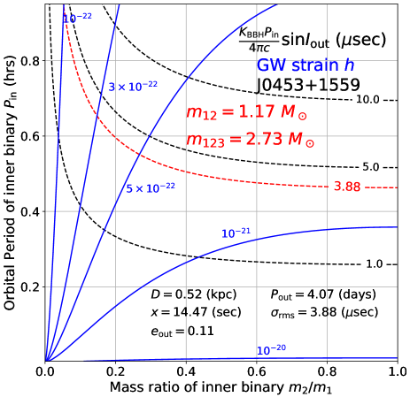
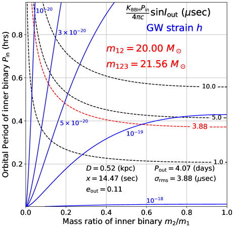
Figure 7: Characteristic amplitudes of the Rømer delay induced by the inner-binary perturbation (dashed black and red lines) and the gravitational wave strain $h$ (solid blue line) as the function of inner-binary orbital period $P_{\mathrm{in}}$ and mass ratio $m_{2}/m_{1}$. The left and right panels show the constraints for J0453+1559 and a hypothetical inner BBH with $m_{12}=20~{}M_{\odot}$, respectively.

As a specific example, we consider the DNS binary J0453+1559, and assume that it is indeed a triple with the unseen companion being a coplanar near-circular inner compact binary of the mass ratio $m_{2}/m_{1}$ and the orbital period $P_{\mathrm{in}}$, instead of a single neutron star. The left panel of Figure 7 plots the amplitudes of the corresponding GW strain (thick solid lines) and the Rømer delay modulation (thin dashed lines). The region above the red line $P_{\mathrm{in}}>P_{\mathrm{in},\mathrm{max}}$ is excluded because it should exhibit the arrival time modulation larger than the observed $\sigma_{\rm rms}$. Interestingly, the region below the limit indicates that the GW strain at the frequency corresponding to $4\pi/P_{\mathrm{in},\mathrm{max}}$ amounts to $h>10^{-21}$ that may be detectable including LISA, DECIGO, and BBO; see Figure 8 below.

Assuming that each DNS system has an equal-mass circular inner binary, we can put rough constraints on the properties of the possible inner binaries. The GW emission merger time $t_{\mathrm{merge}}(P_{\mathrm{in}})$ for an equal-mass circular binary is (Peters, 1964)

$$t_{\mathrm{merge}}(P_{\mathrm{in}})=\frac{5}{64}\left(\frac{\mathcal{G}m_{12}}{c^{3}}\right)^{-5/3}\left(\frac{P_{\mathrm{in}}}{2\pi}\right)^{8/3}\approx 3.92\times 10^{7}\left(\frac{P_{\mathrm{in}}}{\mathrm{hrs}}\right)^{8/3}\left(\frac{m_{12}}{M_{\odot}}\right)^{-5/3}~{}\mathrm{yrs}.$$ (38)

Table 3 summarizes the upper limit on the inner binary period $P_{\mathrm{in},\mathrm{max}}$, the corresponding GW strain $h(4\pi/P_{\mathrm{in},\mathrm{max}})$, and the GW emission merger time $t_{\mathrm{merge}}(P_{\mathrm{in},\mathrm{max}})$.

In order to examine the feasibility to constrain the inner BBH in triple systems, we assume exactly the same triple parameters for the DNS binary J0453+1559 except that the inner companion mass is $m_{12}=20~{}M_{\odot}$. The amplitudes of the Rømer delay modulation and the GW strain for the hypothetical system are plotted in the right panel of Figure 7. Since the GW strain becomes about two orders of magnitude larger compared with the left panel, an inner BBH, if exists at all, would be detected for almost all the the parameter space with either the precise high-cadence pulsar timing or the low-frequency GW observation.

Figure 8 plots the characteristic GW strain $h(4\pi/P_{\mathrm{in}})$ for hypothetical circular inner binaries; long-dashed, short-dashed, dotted and dash-dotted lines corresponds to the inner BBHs of $(m_{1},m_{2})$ $=(30~{}M_{\odot},30~{}M_{\odot})$, $(10~{}M_{\odot},10~{}M_{\odot})$, $(15~{}M_{\odot},5~{}M_{\odot})$, and $(5~{}M_{\odot},5~{}M_{\odot})$, located at $D=10$ kpc from us. Solid lines indicate $h(4\pi/P_{\mathrm{in}})$ from the existing DNS systems shown in Table 3, assuming an equal-mass circular inner binary instead of the companion neutron star. We also show the expected LISA sensitivity curve in 4 year mission (Robson et al., 2019), the expected sky-averaged sensitivity curves of DECIGO and BBO (Yagi & Seto, 2011, 2017), and the aLIGO sensitivity curve from a technical note T1800044-v5 (Barsotti et al., 2018). The figure shows that very short-period inner binary companions are already excluded by non-detection with aLIGO, and the other space-based missions (LISA, DECIGO, and BBO) have enough sensitivity to detect an inner binary with hr-scale orbital period in the future.

Clearly, the joint analysis of the pulsar timing and GW observation is very effective, and can constrain the presence of an unseen inner binary in a complementary fashion; inner BBHs with a shorter orbital period that cannot be probed by the pulsar timing analysis will be detectable by future space-based GW detectors such as LISA, DECIGO, and BBO. Additionally, very short-period inner binaries with sub-second orbital periods can be already probed or constrained by current ground-based GW detectors such as aLIGO.

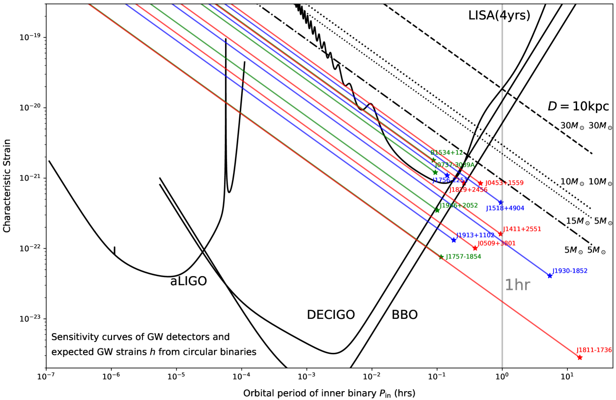
Figure 8: The sensitivity curves of three future space-based GW detectors (LISA, DECIGO, and BBO) and a present ground-based GW detector (aLIGO). The characteristic GW strains $h(4\pi/P_{\mathrm{in}})$ are also plotted for hypothetical inner circular BBHs located at $10$ kpc, and assumed equal-mass circular inner binary companions in the currently known DNS systems. The stars represent the upper limit of inner orbital periods and corresponding GW strains (see Table 3). The DNS systems J1753-2240 and B1913+16 are not plotted in this figure since no constraints are available for these systems. All the results presented here assume that the GW modulations in frequency and phase by the outer orbit are properly subtracted by the predetermined outer orbital parameters.

5 Conclusion

According to the proposed formation scenarios of binary black holes (BBHs), there should be abundant wide-orbit progenitor BBHs in the universe. In the previous papers (Papers I and II), we examine the feasibility to identify such BBHs in triples by detecting short- and long-term radial velocity modulations of a tertiary star induced by the inner-binary perturbation.

In this paper, we consider a pulsar-inner BBH triple, and propose a methodology to search for an inner hidden BBH on the basis of the pulsar arrival time analysis. While the presence of such triples is currently uncertain, if such a triple exists, high precision and cadence pulsar timing can clearly detect a BBH inside distant triples beyond several kpc, inaccessible with the radial velocity observation.

We show that an inner hidden BBH can be identified by the short-term Rømer delay modulation by the inner-binary perturbation with roughly half an inner-binary orbital period. The analytic expression reveals that the modulation has sufficient amplitude for the detection up to $\sim 50$ msec, for our fiducial case of an equal-mass coplanar near-circular inner BBH with $m_{12}=20~{}M_{\odot}$, $P_{\mathrm{in}}=10$ days, and $P_{\mathrm{out}}=100$ days. We also show that the mass of each body and orbital parameters of a triple can be unambiguously determined combining the relativistic time delays, especially the Shapiro delay up to $\sim$ msec for a nearly edge-on system.

As an application of our methodology, we perform a proof-of-concept analysis, and put rough constraints on possible inner binary companions of existing double neutron-star binaries (DNS) using the root mean square of the residuals in observational arrival timing data. We find that our proposed methodology has the sensitivity even on inner binaries with relatively short orbital periods down to $\sim$ hrs when $P_{\mathrm{out}}<O(1)$ day and the pulsar timing precision is on the order of $\mu$sec. While it is unlikely that existing DNS systems actually have inner binary companions instead of singles, the result indicates that our methodology can probe various inner binaries, which may be hardly detected with radial velocity observation.

Additionally, the result implies the possibility of our methodology as a complementary method to the direct gravitational wave (GW) observations. Inner BBHs with $\lesssim 1$ hr orbital period located at $\lesssim 10$ kpc produce the GW strains detectable by future space-based GW detectors including LISA, DECIGO, and BBO, and very short-period inner BBHs with sub-second orbital periods can be already probed by the current ground-based GW detectors such as aLIGO. Therefore, the combination of our methodology with current and future GW observations will provide a potential technique to search for inner BBHs in the near future.

Although we concentrate on the short-term modulation induced by the inner-binary perturbation in this paper, the long-term effects on the time delay such as the Kozai-Lidov oscillations in non-coplanar triples would also provide the feasible methodology to detect inner BBHs, as same as the radial velocity (see Paper II).

The dynamics of triple systems we applied in this paper is quite generic, and can be applied to various other interesting systems, apart from a pulsar-inner BBH triple. For instance, the formation of binary planets in exoplanetary systems via gravitational scattering is predicted theoretically (e.g. Ochiai et al., 2014), and the search through the transit observation is currently proposed (e.g. Lewis et al., 2015). Although the modulation of the tertiary motion induced by a binary planet should be generally small, high precision pulsar timing may be possible to detect the tiny modulation if a tertiary is a pulsar. Adapting our methodology to searching for a binary planet around a pulsar will be one possible application.

In the near future, the space-based GW detectors will start operating and open a new window for the compact object survey. In Figure 8, we show a possible constraint on assumed inner binaries inside triples from the upcoming such detectors. The non-trivial assumption underlying the plot is that the GW modulation due to the outer orbit can be precisely subtracted. For that purpose, it is required to develop a data processing algorithm to detect the GW signals from triple systems. Obviously such a pipeline can be applied not only to pulsar-BBH triples that we have examined in the present paper, but also to BH triple systems. For example, Gupta et al. (2020) considered the GW signals from an inner binary with a wide-separation tertiary undergoing the Kozai-Lidov oscillation. For more compact BH triple systems, however, the resulting GW signals would show more complicated behavior since the GWs from both inner and outer orbits may enter the detectors simultaneously, and it is challenging to disentangle the two components under the situation that three BHs are strongly interacted in tightly packed systems. Nevertheless, such directions should be very important and rewarding since they would lead to the first detection of tight BH triples hidden somewhere in the universe.

Finally, we would like to emphasize that the methodology proposed here is not just a theoretical idea, but an observationally feasible methodology for searching for otherwise unseen astrophysical objects. Theoretically, it is estimated that there are $10^{8}-10^{9}$ stellar mass black holes in our Galaxy (e.g. Shapiro & Teukolsky, 1983), and currently there are many proposals to search for star - black hole binaries with Gaia(e.g. Kawanaka et al., 2016; Breivik et al., 2017; Mashian & Loeb, 2017; Yamaguchi et al., 2018; Shikauchi et al., 2020) and TESS (e.g. Masuda & Hotokezaka, 2019). LIGO’s continuous detection of merger events (e.g. Abbott et al., 2016, 2020) implies that abundant black holes may form BBHs, and still stay in the universe before coalescence. In the near future, the methodology proposed here becomes practically useful in detecting such not-yet-known astronomical objects.

Appendix A The modulation on the Kepler motion induced by the inner-binary perturbation

In order to clearly detect the Rømer delay induced by the inner-binary perturbation, it is important to precisely determine the Keplerian motion and properly subtract it from the timing data. In this section, we briefly discuss how the Keplerian motion is modulated and the best-fit parameters of the Keplerian orbit can be interpreted under the presence of the inner-binary perturbation. For simplicity, we only consider a coplanar near-circular triple and extend the discussion in our previous paper (Paper II).

Following Morais & Correia (2008) and Paper II, the radial Keplerian motion under the inner-binary perturbation is written by the unperturbed Keplerian term $z^{(0)}_{\mathrm{Kep}}(t)$ and the tiny correction $\delta z_{\mathrm{Kep}}(t)$ as

$$z_{\mathrm{Kep}}(t) = z^{(0)}_{\mathrm{Kep}}(t)+\delta z_{\mathrm{Kep}}(t)$$ (A1)

$$= \frac{m_{12}}{m_{123}}a_{\mathrm{out}}\left[1+\frac{3}{4}\frac{m_{1}m_{2}}{m_{12}^{2}}\left(\frac{a_{\mathrm{in}}}{a_{\mathrm{out}}}\right)^{2}\right]\sin{I_{\mathrm{out}}}\sin(\nu_{\mathrm{out}}t+f_{\mathrm{out},0}+\omega_{\mathrm{out}}),$$

where $\nu_{\mathrm{out}}$ and $\omega_{\mathrm{out}}$ denote the mean motion and argument of pericenter of the tertiary pulsar, and $f_{\mathrm{out},0}$ is the initial true anomaly at $t=0$. Since the outer orbit in a triple system should have a non-vanishing eccentricity due to the inner-binary perturbation, $\omega_{\mathrm{out}}$ in the above expressions is generally well defined. The above expression shows the amplitude of the radial Keplerian motion is modulated by the inner-binary perturbation with the order of $(a_{\mathrm{in}}/a_{\mathrm{out}})^{2}$.

The averaged orbital period $P^{(\mathrm{ave})}_{\mathrm{out}}$ over a orbital motion is also modulated due to the long-term effects of the inner-binary perturbation. Since $\omega_{\mathrm{out}}$ and $f_{\mathrm{out},0}$ are not constant with time under the perturbation, the angular frequency corresponding to the averaged orbital period is written as

$$\nu^{(\mathrm{ave})}_{\mathrm{out}}\equiv\frac{2\pi}{P^{(\mathrm{ave})}_{\mathrm{out}}}\approx\nu_{\mathrm{out}}+\dot{\omega}_{\mathrm{out}}+\dot{f}_{\mathrm{out},0}.$$ (A2)

The $\dot{\omega}_{\mathrm{out}}$ and $\dot{f}_{\mathrm{out},0}$ can be calculated by the Lagrange planetary equations using the orbit-averaged quadrupole Hamiltonian of triple system. The orbit-averaged quadrupole Hamiltonian $\bar{F}$ is given by (e.g., Morais & Correia, 2012):

$$\bar{F} = C_{\mathrm{quad}}[2-12e_{\mathrm{in}}^{2}-6(1-e_{\mathrm{in}}^{2})(\sin{I_{\mathrm{in}}}\sin{I_{\mathrm{out}}}\cos(\Delta\Omega)+\cos{I_{\mathrm{in}}}\cos{I_{\mathrm{out}}})^{2}+30e_{\mathrm{in}}^{2}$$ (A4)

$$\times(-\sin{I_{\mathrm{out}}}\cos{I_{\mathrm{in}}}\sin{\omega_{\mathrm{in}}}\cos(\Delta\Omega)-\sin{I_{\mathrm{out}}}\cos{\omega_{\mathrm{in}}}\sin(\Delta\Omega)+\sin{I_{\mathrm{in}}}\sin{\omega_{\mathrm{in}}}\cos{I_{\mathrm{out}}})^{2}],$$

where

$$C_{\mathrm{quad}}\equiv\frac{\mathcal{G}}{16}\frac{m_{1}m_{2}}{m_{12}}\frac{m_{3}}{(1-e_{\mathrm{out}}^{2})^{3/2}}\left(\frac{a_{\mathrm{in}}^{2}}{a_{\mathrm{out}}^{3}}\right)~{}~{}~{}\mathrm{and}~{}~{}~{}\Delta\Omega\equiv\Omega_{\mathrm{in}}-\Omega_{\mathrm{out}}.$$ (A5)

The Lagrange planetary equations of $\omega_{\mathrm{out}}$ and $f_{\mathrm{out},0}$ are (see e.g. Danby, 1988)

$$\dot{\omega}_{\mathrm{out}} = -\frac{\sqrt{1-e_{\mathrm{out}}^{2}}}{\mu_{\mathrm{out}}\nu_{\mathrm{out}}a_{\mathrm{out}}^{2}e_{\mathrm{out}}}\frac{\partial\bar{F}}{\partial e_{\mathrm{out}}}+\frac{\cos{I_{\mathrm{out}}}}{\mu_{\mathrm{out}}\nu_{\mathrm{out}}a_{\mathrm{out}}^{2}\sqrt{1-e_{\mathrm{out}}^{2}}\sin{I_{\mathrm{out}}}}\frac{\partial\bar{F}}{\partial I_{\mathrm{out}}}$$ (A6)

and

$$\dot{f}_{\mathrm{out},0} \approx \dot{\bar{M}}_{\mathrm{out},0}=\frac{1-e_{\mathrm{out}}^{2}}{\mu_{\mathrm{out}}\nu_{\mathrm{out}}a_{\mathrm{out}}^{2}e_{\mathrm{out}}}\frac{\partial\bar{F}}{\partial e_{\mathrm{out}}}+\frac{2}{\mu_{\mathrm{out}}\nu_{\mathrm{out}}a_{\mathrm{out}}}\frac{\partial\bar{F}}{\partial a_{\mathrm{out}}},$$ (A7)

where $\mu_{\mathrm{out}}\equiv m_{3}m_{12}/m_{123}$. The $\bar{M}_{\mathrm{out},0}$ is defined by the mean anomaly $M_{\mathrm{out}}$ to avoid the secular term in the equation as

$$M_{\mathrm{out}}\equiv\nu_{\mathrm{out}}(t-t_{0})+M_{\mathrm{out},0}\equiv\int^{t}_{t_{0}}{\nu_{\mathrm{out}}dt}+\bar{M}_{\mathrm{out},0},$$ (A8)

where $t_{0}$ is the initial time. Note that we use the fact that the initial true anomaly is well approximated by the initial mean anomaly for a near-circular case. Substituting the equation (A4) into the Lagrange planetary equations, and neglect the outer eccentricity $e_{\mathrm{out}}$, we obtain

$$\dot{\omega}_{\mathrm{out}}\approx\frac{12C_{\mathrm{quad}}}{\mu_{\mathrm{out}}\nu_{\mathrm{out}}a_{\mathrm{out}}^{2}}~{}~{}~{}\mathrm{and}~{}~{}~{}\dot{f}_{\mathrm{out},0}\approx\frac{12C_{\mathrm{quad}}}{\mu_{\mathrm{out}}\nu_{\mathrm{out}}a_{\mathrm{out}}^{2}}.$$ (A9)

Therefore, the averaged orbital period $P^{(\mathrm{ave})}_{\mathrm{out}}$ over a orbital motion is approximated as

$$\frac{P^{(\mathrm{ave})}_{\mathrm{out}}}{P_{\mathrm{out}}}\approx\frac{2\pi}{\nu_{\mathrm{out}}+\dot{\omega}_{\mathrm{out}}+\dot{f}_{\mathrm{out},0}}\approx 1-\frac{2\dot{\omega}_{\mathrm{out}}P_{\mathrm{out}}}{2\pi}.$$ (A10)

Incidentally, Figure 4 in Paper II indicated the factor 2 difference between $P_{\mathrm{out}}$ and $P^{(\mathrm{ave})}_{\mathrm{out}}$, but it is due to the additional contribution from $\dot{f}_{\mathrm{out},0}$ that was omitted in Paper II. Thus the above equation (A10) correctly reproduces the numerical result from analytic computation.

References

- Abbott et al. (2016) Abbott, B. P., Abbott, R., Abbott, T. D., et al. 2016, Physical Review Letters, 116, 061102, doi: 10.1103/PhysRevLett.116.061102
- Abbott et al. (2020) Abbott, R., Abbott, T. D., Abraham, S., et al. 2020, ApJ, 896, L44, doi: 10.3847/2041-8213/ab960f
- Amaro-Seoane et al. (2017) Amaro-Seoane, P., Audley, H., Babak, S., et al. 2017, arXiv e-prints, arXiv:1702.00786. https://arxiv.org/abs/1702.00786
- Backer & Hellings (1986) Backer, D. C., & Hellings, R. W. 1986, ARA&A, 24, 537, doi: 10.1146/annurev.aa.24.090186.002541
- Barsotti et al. (2018) Barsotti, L., Gras, S., Evans, M., & Fritschel, P. 2018, The updated Advanced LIGO design curve, Tech. Rep. LIGO-T1800044-v5, LIGO
- Belczynski et al. (2016) Belczynski, K., Holz, D. E., Bulik, T., & O’Shaughnessy, R. 2016, Nature, 534, 512, doi: 10.1038/nature18322
- Belczynski et al. (2002) Belczynski, K., Kalogera, V., & Bulik, T. 2002, ApJ, 572, 407, doi: 10.1086/340304
- Breivik et al. (2017) Breivik, K., Chatterjee, S., & Larson, S. L. 2017, ApJ, 850, L13, doi: 10.3847/2041-8213/aa97d5
- Cameron et al. (2018) Cameron, A. D., Champion, D. J., Kramer, M., et al. 2018, Monthly Notices of the Royal Astronomical Society: Letters, 475, L57, doi: 10.1093/mnrasl/sly003
- Corongiu et al. (2007) Corongiu, A., Kramer, M., Stappers, B. W., et al. 2007, A&A, 462, 703, doi: 10.1051/0004-6361:20054385
- Cunha et al. (2018) Cunha, J. V., Silva, F. E., & Lima, J. A. S. 2018, MNRAS, 480, L28, doi: 10.1093/mnrasl/sly113
- Danby (1988) Danby, J. M. A. 1988, Fundamentals of celestial mechanics (Willmann-Bell, Inc.)
- Demorest et al. (2010) Demorest, P. B., Pennucci, T., Ransom, S. M., Roberts, M. S. E., & Hessels, J. W. T. 2010, Nature, 467, 1081, doi: 10.1038/nature09466
- Edwards et al. (2006) Edwards, R. T., Hobbs, G. B., & Manchester, R. N. 2006, MNRAS, 372, 1549, doi: 10.1111/j.1365-2966.2006.10870.x
- Ferdman et al. (2014) Ferdman, R. D., Stairs, I. H., Kramer, M., et al. 2014, Monthly Notices of the Royal Astronomical Society, 443, 2183, doi: 10.1093/mnras/stu1223
- Ferdman et al. (2020) Ferdman, R. D., Freire, P. C. C., Perera, B. B. P., et al. 2020, Nature, 583, 211, doi: 10.1038/s41586-020-2439-x
- Fonseca et al. (2014) Fonseca, E., Stairs, I. H., & Thorsett, S. E. 2014, The Astrophysical Journal, 787, 82, doi: 10.1088/0004-637x/787/1/82
- Fragione et al. (2020) Fragione, G., Martinez, M. A. S., Kremer, K., et al. 2020, arXiv e-prints, arXiv:2007.11605. https://arxiv.org/abs/2007.11605
- Gupta et al. (2020) Gupta, P., Suzuki, H., Okawa, H., & Maeda, K.-i. 2020, Phys. Rev. D, 101, 104053, doi: 10.1103/PhysRevD.101.104053
- Haniewicz et al. (2020) Haniewicz, H. T., Ferdman, R. D., Freire, P. C. C., et al. 2020, arXiv e-prints, arXiv:2007.07565. https://arxiv.org/abs/2007.07565
- Harry et al. (2006) Harry, G. M., Fritschel, P., Shaddock, D. A., Folkner, W., & Phinney, E. S. 2006, Classical and Quantum Gravity, 23, 4887, doi: 10.1088/0264-9381/23/15/008
- Hartle (2003) Hartle, J. B. 2003, Gravity : an introduction to Einstein’s general relativity (Pearson)
- Hayashi & Suto (2020) Hayashi, T., & Suto, Y. 2020, ApJ, 897, 29, doi: 10.3847/1538-4357/ab97ad
- Hayashi et al. (2020) Hayashi, T., Wang, S., & Suto, Y. 2020, The Astrophysical Journal, 890, 112, doi: 10.3847/1538-4357/ab6de6
- Janssen et al. (2008) Janssen, G. H., Stappers, B. W., Kramer, M., et al. 2008, A&A, 490, 753, doi: 10.1051/0004-6361:200810076
- Kawanaka et al. (2016) Kawanaka, N., Yamaguchi, M., Piran, T., & Bulik, T. 2016, Proceedings of the International Astronomical Union, 12, 41, doi: 10.1017/S1743921316012606
- Keith et al. (2009) Keith, M. J., Kramer, M., Lyne, A. G., et al. 2009, Monthly Notices of the Royal Astronomical Society, 393, 623, doi: 10.1111/j.1365-2966.2008.14234.x
- Kramer et al. (2006) Kramer, M., Stairs, I. H., Manchester, R. N., et al. 2006, Science, 314, 97, doi: 10.1126/science.1132305
- Lewis et al. (2015) Lewis, K. M., Ochiai, H., Nagasawa, M., & Ida, S. 2015, ApJ, 805, 27, doi: 10.1088/0004-637X/805/1/27
- Lynch et al. (2018) Lynch, R. S., Swiggum, J. K., Kondratiev, V. I., et al. 2018, The Astrophysical Journal, 859, 93, doi: 10.3847/1538-4357/aabf8a
- Mardling & Aarseth (1999) Mardling, R., & Aarseth, S. 1999, in NATO Advanced Science Institutes (ASI) Series C, Vol. 522, NATO Advanced Science Institutes (ASI) Series C, ed. B. A. Steves & A. E. Roy (Springer), 385
- Martinez et al. (2015) Martinez, J. G., Stovall, K., Freire, P. C. C., et al. 2015, The Astrophysical Journal, 812, 143, doi: 10.1088/0004-637x/812/2/143
- Martinez et al. (2017) —. 2017, The Astrophysical Journal, 851, L29, doi: 10.3847/2041-8213/aa9d87
- Mashian & Loeb (2017) Mashian, N., & Loeb, A. 2017, MNRAS, 470, 2611, doi: 10.1093/mnras/stx1410
- Masuda & Hotokezaka (2019) Masuda, K., & Hotokezaka, K. 2019, ApJ, 883, 169, doi: 10.3847/1538-4357/ab3a4f
- Morais & Correia (2008) Morais, M. H. M., & Correia, A. C. M. 2008, A&A, 491, 899, doi: 10.1051/0004-6361:200810741
- Morais & Correia (2011) —. 2011, A&A, 525, A152, doi: 10.1051/0004-6361/201014812
- Morais & Correia (2012) —. 2012, MNRAS, 419, 3447, doi: 10.1111/j.1365-2966.2011.19986.x
- Nelemans et al. (2001) Nelemans, G., Yungelson, L. R., & Portegies Zwart, S. F. 2001, A&A, 375, 890, doi: 10.1051/0004-6361:20010683
- Ochiai et al. (2014) Ochiai, H., Nagasawa, M., & Ida, S. 2014, ApJ, 790, 92, doi: 10.1088/0004-637X/790/2/92
- Peters (1964) Peters, P. C. 1964, Physical Review, 136, 1224, doi: 10.1103/PhysRev.136.B1224
- Portegies Zwart & McMillan (2000) Portegies Zwart, S. F., & McMillan, S. L. W. 2000, ApJ, 528, L17, doi: 10.1086/312422
- Raghavan et al. (2010) Raghavan, D., McAlister, H. A., Henry, T. J., et al. 2010, ApJS, 190, 1, doi: 10.1088/0067-0049/190/1/1
- Ransom et al. (2014) Ransom, S. M., Stairs, I. H., Archibald, A. M., et al. 2014, Nature, 505, 520, doi: 10.1038/nature12917
- Robson et al. (2019) Robson, T., Cornish, N. J., & Liu, C. 2019, Classical and Quantum Gravity, 36, 105011, doi: 10.1088/1361-6382/ab1101
- Sana et al. (2012) Sana, H., de Mink, S. E., de Koter, A., et al. 2012, Science, 337, 444, doi: 10.1126/science.1223344
- Sasaki et al. (2016) Sasaki, M., Suyama, T., Tanaka, T., & Yokoyama, S. 2016, Physical Review Letters, 117, 061101, doi: 10.1103/PhysRevLett.117.061101
- Sato et al. (2017) Sato, S., Kawamura, S., Ando, M., et al. 2017, in Journal of Physics Conference Series, Vol. 840, Journal of Physics Conference Series, 012010, doi: 10.1088/1742-6596/840/1/012010
- Schutz (2009) Schutz, B. 2009, A First Course in General Relativity (Cambridge University Press)
- Shapiro & Teukolsky (1983) Shapiro, S. L., & Teukolsky, S. A. 1983, Black holes, white dwarfs, and neutron stars : the physics of compact objects (A Wiley-Interscience Publication, New York: Wiley, 1983)
- Shikauchi et al. (2020) Shikauchi, M., Kumamoto, J., Tanikawa, A., & Fujii, M. S. 2020, PASJ, doi: 10.1093/pasj/psaa030
- Stovall et al. (2018) Stovall, K., Freire, P. C. C., Chatterjee, S., et al. 2018, The Astrophysical Journal, 854, L22, doi: 10.3847/2041-8213/aaad06
- Swiggum et al. (2015) Swiggum, J. K., Rosen, R., McLaughlin, M. A., et al. 2015, The Astrophysical Journal, 805, 156, doi: 10.1088/0004-637x/805/2/156
- Taylor & Weisberg (1982) Taylor, J. H., & Weisberg, J. M. 1982, ApJ, 253, 908, doi: 10.1086/159690
- Toonen et al. (2016) Toonen, S., Hamers, A., & Portegies Zwart, S. 2016, Computational Astrophysics and Cosmology, 3, 6, doi: 10.1186/s40668-016-0019-0
- Weisberg & Taylor (2005) Weisberg, J. M., & Taylor, J. H. 2005, in Astronomical Society of the Pacific Conference Series, Vol. 328, Binary Radio Pulsars, ed. F. A. Rasio & I. H. Stairs, 25. https://arxiv.org/abs/astro-ph/0407149
- Wong et al. (2019) Wong, K. W. K., Berti, E., Gabella, W. E., & Holley-Bockelmann, K. 2019, MNRAS, 483, L33, doi: 10.1093/mnrasl/sly208
- Yagi & Seto (2011) Yagi, K., & Seto, N. 2011, Phys. Rev. D, 83, 044011, doi: 10.1103/PhysRevD.83.044011
- Yagi & Seto (2017) —. 2017, Phys. Rev. D, 95, 109901, doi: 10.1103/PhysRevD.95.109901
- Yamaguchi et al. (2018) Yamaguchi, M. S., Kawanaka, N., Bulik, T., & Piran, T. 2018, ApJ, 861, 21, doi: 10.3847/1538-4357/aac5ec