Approximate cross-validated mean estimates for Bayesian hierarchical regression models

Abstract

We introduce a novel procedure for obtaining cross-validated predictive estimates for Bayesian hierarchical regression models (BHRMs). BHRMs are popular for modeling complex dependence structures (e.g., Gaussian processes and Gaussian Markov random fields) but can be computationally expensive to run. Cross-validation (CV) is, therefore, not a common practice to evaluate the predictive performance of BHRMs. Our method circumvents the need to re-run computationally costly estimation methods for each cross-validation fold and makes CV more feasible for large BHRMs. We shift the CV problem from probability-based sampling to a familiar and straightforward optimization problem by conditioning on the variance-covariance parameters. Our approximation applies to the leave-one-out CV and the leave-one-cluster-out CV, the latter of which is more appropriate for models with complex dependencies. In many cases, this produces estimates equivalent to the full CV. We provide theoretical results, demonstrate the efficacy of our method on publicly available data and in simulations, and compare the model performance with several competing methods for CV approximation.

Keywords: Bayesian hierarchical regression model, multi-level model, leave-one-out, leave-cluster-out, plug-in estimator

1 Introduction

Bayesian hierarchical regression models (BHRMs) are often used to model complex dependence structures while producing probabilistic uncertainty estimates. Except for the simplest models, BHRMs require computationally expensive methods such as Markov Chain Monte Carlo (MCMC) to obtain the posterior density. It has led to many papers that either present new methods to approximate the posterior density (e.g., Kingma and Welling, 2013; Lewis and Raftery, 1997; Rue et al., 2009) or attempt to make current methods more efficient (Bardenet et al., 2017; Korattikara et al., 2014; Quiroz et al., 2019).

The computational cost of BHRM increases by an order of magnitude when we need to repeat the posterior density estimation process for each fold of the cross-validation (CV). A common approach for cross-validation is to randomly partition the data into $K$ equally-sized subsets, called $K$-fold CV. Reducing the number of CV folds, $K$, can mitigate the cost of cross-validation. However, when the data are not independent of each other, random $K$-fold cross-validation can select models which overfit because of the high correlation between test and training data (Arlot et al., 2010; Opsomer et al., 2001). Models with repeated measures are one such example, where the correlation between repeated samples from the same unit means that random $K$-fold cross-validation can select models which overfit the unit-specific effects. This produces over-optimistic estimates of the selected model’s performance on a new unit. CV dropping out whole clusters (possibly more than one) at a time would be the most robust, but it often requires far more than 10 CV folds.

We reduce the computational cost of BHRM in the CV setting by introducing a novel procedure for obtaining BHRM posterior mean estimates. We use the full-data posterior mean of the variance-covariance parameters as a plug-in estimator and re-estimate all other model parameters given the training data and the plug-in estimate. Our method is motivated by Kass and Steffey (1989) who approximated the posterior mean $E(X\beta|Y)$ using the conditional mean given the estimated variance terms. Our extensions include (1) approximating hyperparameters in the CV setting, (2) allowing the model to have random effects with any dependence structure, (3) extending the approximation from Bayesian hierarchical linear regression models to generalized linear mixed models, and (4) considering the leave-one-cluster-out CV which is more appropriate for models with complex dependency. We show with multiple datasets that our method produces more stable estimates than other competing methods while keeping computation time reasonable.

In Section 2, we introduce our procedure, which we refer to as AXE, an abbreviation for (A)pproximate (X)cross-validation (E)stimates. It can be applied to linear mixed models and generalized linear mixed models, and many CV schemas, e.g., $K$-fold, leave-one-out (LOO), and leave-one-cluster-out (LCO). We also discuss AXE’s asymptotic properties and finite sample behavior. In Section 3, we summarize competing methods for CV approximation and extend some so that they can be applicable to LCO-CV. Section 4 presents and discusses empirical results comparing the manual cross-validation (MCV) and different approximate CV estimates using a variety of publicly available data sets. In Section 5, we summarize the method and our findings.

2 Approximate cross-validation estimates using plug-in estimators (AXE)

Section 2.1 presents the AXE procedure in the linear regression setting. Section 2.2 presents the AXE procedure in the generalized linear regression setting, which requires an additional approximation. A particular challenge in the LCO-CV approximation is that all observations informing the estimation of the random effect are associated with the test data which we describe in detail in Section 2.3. Section 2.4 describes the large-sample behavior of AXE estimates. Section 2.5 provides a finite-sample diagnostic, which we call AXE+.

We introduce the notation used throughout the paper. Let $Y\in I\!\!R^{N}$ denote a continuous response vector and $X\in I\!\!R^{N\times P}$ denote the design matrix. For the $J$-fold cross-validation, $j=1,\dots,J$ indicates the cross-validation folds; $\mathpzc{s}_{j}$ corresponds to the indices of the held-out data for CV fold $j$; $n_{j}$ is the corresponding sample size; $Y_{\mathpzc{s}_{j}}\in I\!\!R^{n_{j}}$ is the test response data; $Y_{-\mathpzc{s}_{j}}\in I\!\!R^{N-n_{j}}$ the training response data; and similarly $X_{\mathpzc{s}_{j}}\in I\!\!R^{n_{j}\times P}$ refers to the rows of $X$ indexed by $\mathpzc{s}_{j}$, while $X_{-\mathpzc{s}_{j}}\in I\!\!R^{(N-n_{j})\times P}$ refers to the remaining rows of $X$ without $X_{\mathpzc{s}_{j}}$. We denote the transpose of a matrix (or vector) $A$ as $A^{\prime}$.

2.1 AXE for linear mixed models

In linear mixed models (LMM), the continuous response vector, $Y$, follows

$$Y|\beta,\phi\sim N(X\beta,\phi^{2}),$$ (1)

where $X$ are the non-random covariates, $\beta\coloneqq(\beta_{1}^{\prime},\beta_{2}^{\prime})^{\prime}\in I\!\!R^{P}$ includes fixed effects $\beta_{1}$ and random effects $\beta_{2}$, $\phi\in I\!\!R^{+}$ is a positive scalar.

$$\begin{split}\beta\sim N\left(\alpha,\begin{bmatrix}C&0\\ 0&\Sigma\end{bmatrix}\right),\\ \Sigma\sim f_{\Sigma}(\Sigma),\quad\phi\sim f_{\phi}(\phi),\end{split}$$ (2)

where $C\in I\!\!R^{P_{1}\times P_{1}}$ is a fixed positive-definite matrix and often a diagonal matrix with large positive values. The hyperparameters, $\Sigma\in I\!\!R^{P_{2}\times P_{2}}$, can take many forms, as long as it is positive-definite, e.g., models with Gaussian Markov random fields sample from the space of all possible $\Sigma$’s such that a variable in $\beta_{2}$ is independent of all others, given its neighborhood. We take $\alpha=0$ throughout this paper without loss of generality.

The posterior mean for $\beta$ conditioned on variance parameters has the form

$$E[\beta|\Sigma,\phi,Y]=\phi^{-2}VX^{\prime}Y,\quad V=\left(\phi^{-2}X^{\prime}X+\begin{bmatrix}C^{-1}&0\\ 0&\Sigma^{-1}\end{bmatrix}\right)^{-1},$$ (3)

which is analogous to the form of a Frequentist linear regression. We propose to use the full-data posterior mean estimates $\hat{\Sigma}=E[\Sigma|Y]$ and $\hat{\phi}=E[\phi|Y]$ as plug-in estimators in (3) to derive cross-validated mean estimates. In the linear regression setting, this results in a simple and straightforward closed-form solution for the cross-validated mean estimates:

$$\hat{Y}_{\mathpzc{s}_{j}}^{\text{AXE}}=E[X_{\mathpzc{s}_{j}}\beta|Y_{-\mathpzc{s}_{j}},\hat{\Sigma},\hat{\phi}]=\hat{\phi}^{-2}X_{\mathpzc{s}_{j}}\left(\hat{\phi}^{-2}X_{-\mathpzc{s}_{j}}^{\prime}X_{-\mathpzc{s}_{j}}+\begin{bmatrix}C^{-1}&0\\ 0&\hat{\Sigma}^{-1}\end{bmatrix}\right)^{-1}X_{-\mathpzc{s}_{j}}^{\prime}Y_{-\mathpzc{s}_{j}}.$$ (4)

The posterior variance of fixed effects $\beta_{1}$, $C$, is not estimated and is taken as the diagonal matrix of prior variances for $\beta_{1}$. One common practice is to take $C^{-1}$ as the matrix of $0$s, which corresponds to the assumption that the fixed effects have infinite variance.

The AXE procedure in (4) essentially proposes using a Frequentist cross-validation to estimate $E[Y_{\mathpzc{s}_{j}}|Y_{-\mathpzc{s}_{j}}]$ in place of a full Bayesian estimation of the posterior predictive density. AXE is likewise $\mathcal{O}\left(N^{2}P+P^{3}\right)$ in time for each CV fold. In comparison, Gibbs sampling of the same problem (when available) is $\mathcal{O}\left(MN^{3}P+MNP^{2}+MP^{3}\right)$ in time for each CV fold, where $M$ is the number of MCMC iterations.

Our approach relies on the approximation that the conditional expectation of the posterior mean evaluated at the full-data posterior means of the variance parameters, $\hat{\Sigma}=E[\Sigma|Y]$ and $\hat{\phi}=E[\phi|Y]$, approximates the desired posterior predictive mean, i.e., $E[X_{\mathpzc{s}_{j}}\beta|Y_{-\mathpzc{s}_{j}},\hat{\Sigma},\hat{\phi}]\approx E[X_{\mathpzc{s}_{j}}\beta|Y_{-\mathpzc{s}_{j}}]$. This looks similar to the approximation in Kass and Steffey (1989) but here we are in a cross-validation setting and we are plugging in the full-data estimates (as opposed to the training data estimates). In Section 2.4, we show that the approximation holds asymptotically under leave-one-cluster-out cross-validation.

2.2 AXE for generalized linear mixed models

Generalized linear mixed models (GLMMs) assume that $Y|\beta$ is not normally distributed. We follow the approximate inference in GLMM developed by Breslow and Clayton (1993) and derive the corresponding AXE for GLMM. Suppose $Y|\beta$ are independent with some probability density function $\pi$, so that

$$Y_{i}|X_{i}\beta\sim\pi(u_{i},a_{i},\phi^{2},v(u_{i})),$$ (5)

where $E(Y_{i}|X_{i}\beta)=u_{i}$, $\mathrm{var}(Y_{i}|X_{i}\beta)=a_{i}\phi^{2}v(u_{i})$, $a_{i}$ is a known constant, $\phi^{2}$ is a dispersion parameter. The regression model assumes that $g(u_{i})=X_{i}\beta$, where $g(.)$ is the link function and the prior distribution of $\beta$ is specified in (2).

Note that, the normal priors on the coefficients $\beta$ are no longer conjugate, and the analytic solution of (4) is unavailable. Instead, an iterative weighted least square algorithm (IWLS) is commonly used to fit GLM or GLMM (Holland and Welsch, 1977; Green, 1984). Defining a working response,

$$\tilde{Y_{i}}=X_{i}\beta+(Y_{i}-u_{i})g^{\prime}(u_{i}),$$

and a $n\times n$ diagonal weight matrix, $W$, with diagonal terms

$$w_{i}=\{\phi^{2}a_{i}v(u_{i})[g^{\prime}(u_{i})]^{2}\}^{-1},$$

i.e., for the logistic model, $g(u_{i})=\log(u_{i})-\log(1-u_{i})$, $g^{\prime}(u_{i})=\frac{1}{u_{i}(1-u_{i})}$, and $w_{i}=u_{i}(1-u_{i})$; for the Poisson model, $g(u_{i})=\log(u_{i})$, $g^{\prime}(u_{i})=\frac{1}{u_{i}}$, and $w_{i}=u_{i}$. IWLS repeatedly updates the working response vector and the weight matrix until its convergence. Given $W$, Harville (1977) shows that the best linear unbiased estimation (BLUE) of $\beta$ can be obtained from the associated weighted linear model,

$$\tilde{Y}|\beta,\sigma^{2}\sim N(X\beta,W^{-1}).$$

In the cross-validation setting, we approximate the training data weights, $W_{-\mathpzc{s}_{j}}$, by the corresponding weights at the convergence of the full data analysis. It is reasonable under the conditions we present in Section 2.1: 1) $E[X_{\mathpzc{s}_{j}}\beta|\tilde{Y}_{-\mathpzc{s}_{j}},\dot{\Sigma},\dot{\phi}]\approx E[X_{\mathpzc{s}_{j}}\beta|\tilde{Y}_{-\mathpzc{s}_{j}}]$, where $\dot{\Sigma}=E[\Sigma|\tilde{Y}_{-\mathpzc{s}_{j}}]$, $\dot{\phi}=E[\phi|\tilde{Y}_{-\mathpzc{s}_{j}}]$ and 2) $E[\Sigma|\tilde{Y}]\approx\dot{\Sigma}$, $E[\phi|\tilde{Y}]\approx\dot{\phi}$.

We plug in the working response vector, $\tilde{Y}_{-\mathpzc{s}_{j}}$, the weight matrix, $W_{-\mathpzc{s}_{j}}$, and other variance estimates, $\hat{\Sigma}$, in the full data analysis, and obtain the following AXE estimates for the test data working response, $\tilde{Y}_{\mathpzc{s}_{j}}$,

$$\hat{\tilde{Y}}_{\mathpzc{s}_{j}}^{\text{AXE}}=E[X_{\mathpzc{s}_{j}}\beta|\tilde{Y}_{-\mathpzc{s}_{j}},W_{-\mathpzc{s}_{j}},\hat{\Sigma}]=X_{\mathpzc{s}_{j}}\left(X_{-\mathpzc{s}_{j}}^{\prime}W_{-\mathpzc{s}_{j}}X_{-\mathpzc{s}_{j}}+\begin{bmatrix}C^{-1}&0\\ 0&\hat{\Sigma}^{-1}\end{bmatrix}\right)^{-1}X_{-\mathpzc{s}_{j}}^{\prime}W_{-\mathpzc{s}_{j}}\tilde{Y}_{-\mathpzc{s}_{j}}.$$ (6)

Finally, we transform the test data working response to the original scale by $\hat{{Y}}_{\mathpzc{s}_{j}}^{\text{AXE}}=g^{-1}(\hat{\tilde{Y}}_{\mathpzc{s}_{j}}^{\text{AXE}})$. If there is any concern that the weight matrix might differ between the full-data analysis and the training data analysis, then we can run a few more iterations of the IWLS algorithm. We start from the AXE estimates of the working responses and iteratively update the training data weights and the working responses. In practice, $\hat{\tilde{Y}}_{\mathpzc{s}_{j}}^{\text{AXE}}$ without additional IWLS iterations works well.

2.3 Leave-one-cluster-out cross-validation (LCO-CV)

One can apply AXE to any CV design, of which leave-one-out (LOO-CV) and leave-one-cluster-out (LCO-CV) are popular choices. For both LOO-CV and LCO-CV, the number of CV folds can grow with the amount of data, making the computation expensive. Thus they typically benefit the most from CV approximation methods. We focus on proving AXE convergence under LCO-CV, of which LOO-CV is a special case. We first define LCO-CV and related notation. Then, we introduce and discuss existing LCO-CV approximation methods.

In LOO-CV, a single observation is held out as test data for each CV fold, and the number of CV folds equals the number of data points, $N$. LOO-CV is commonly used because it maintains as much similarity to the full data model posterior as possible while evaluating the fit to new data. LCO-CV is often used in models with clustered data and cluster-specific parameters, e.g., the patient-specific random effects in a longitudinal model with $J$ patients. When the data are sampled uniformly at random to form CV folds, data from one patient can be split between the training and test data. It introduces the correlation between the training and test data and can result in overfitting to the patient-specific parameters (Arlot et al., 2010; Opsomer et al., 2001). To fairly evaluate the predictive capability for a new cluster, LCO-CV defines $J$ CV folds corresponding to $J$ clusters and withholds all observations informing the estimation of a cluster-specific random effect.

LCO-CV has been a challenging CV design for the approximate inference. Existing CV approximation methods use the full-data posterior density $f(\beta|Y)$ to approximate the training data posterior density $f(\beta|Y_{-\mathpzc{s}_{j}})$. Under LCO-CV, these approximations can be inaccurate for two reasons. First, since the test data corresponds to the data in a cluster, the test data sample size can be large. It is shown that the larger the sample size of the test data, the more likely it is that the difference in densities $f(\beta|Y)$ and $f(\beta|Y_{-\mathpzc{s}_{j}})$ is large (Gelfand et al., 1992). Second, under cross-validation, the cluster-specific random effects, $\theta_{j}$, cannot be estimated from the training data, relying instead on samples drawn from $\theta_{j}|\theta_{-j},\Sigma$.

To focus on the random effects which pertain to the LCO-CV design, we split $\beta$ into $\theta$ and the remaining coefficients in $\beta$:

$$\beta=(\beta_{/\theta}^{\prime},\hskip 5.0pt\theta^{\prime})^{\prime},$$ (7)

where $\theta$ refers to the part of random effects that pertain to the CV design, and $\beta_{/\theta}$ refers to the components in $\beta$ other than $\theta$, which contain all fixed effects and the part of random effects that do not pertain to the CV design. $\theta\coloneqq(\theta_{1},\theta_{2},\ldots,\theta_{J})^{\prime}\in I\!\!R^{K}$ ($J\leq K\leq P_{2}$). Similarly. we split $X$ column-wise into

$$X=[X_{\beta_{/\theta}}\hskip 5.0ptX_{\theta}],$$ (8)

where $X_{\theta}$ contains the subset of covariates that correspond to $\theta$ and $X_{\beta_{/\theta}}$ contains the remaining columns of $X$.

2.4 Asymptotic behavior under LCO-CV

For the linear mixed models (LMM) case, we first show that the full-data posterior means for variance parameters $\Sigma$ and $\phi$ approximate the training data posterior means; see Theorem 2.1. We then show the convergence of the AXE approximation in Corollary 2.2.

Theorem 2.1.

Let response vector $Y\in I\!\!R^{N}$ of a hierarchical linear regression follow a normal distribution as in (1) and (2) and define $\theta$ as in (7). The data are partitioned into CV folds based on $\theta$, where all data informing $\theta_{j}$ correspond to the test data for CV fold $j$, and $\mathpzc{s}_{j}\subset\{1,\dots,N\}$ is the set of indices for the test data in the $j^{th}$ CV fold. Additionally let $X_{\mathpzc{s}_{j}}=\mathbbm{1}_{n_{j}}x_{j}^{\prime}$ for some vector $x_{j}\in I\!\!R^{P}$, where $\mathbbm{1}_{n_{j}}$ is a vector of $1$s with length $n_{j}$ and $n_{j}$ is the size of $\mathpzc{s}_{j}$, $\mathbbm{1}\in\text{span}(X)$, and prior densities $f_{\Sigma}(\Sigma)$ and $f_{\phi}(\phi)$ such that the resulting posterior is proper. $V$ is defined as in (3). Then $E[\Sigma|Y]=E[\Sigma|Y_{-\mathpzc{s}_{j}}](1+\mathcal{O}_{P}\left(n_{j}/N\right))$ and $E[\phi|Y]=E[\phi|Y_{-\mathpzc{s}_{j}}](1+\mathcal{O}_{P}\left(n_{j}/N\right))$ uniformly across $j$ as $N$ goes to infinity, where the probability in the $\mathcal{O}_{P}{}$ refers to the posterior distribution over $Y$, which also depends on the non-random covariates $X$, and the priors $f_{\Sigma}(\Sigma)$ and $f_{\phi}(\phi)$.

For proof, see Appendix LABEL:appx:proof.

Remark 1.

The requirement that $X_{\mathpzc{s}_{j}}=\mathbbm{1}_{n_{j}}x_{j}^{\prime}$ is a technical one so that an analytical form of the difference in $\ell(\Sigma,\phi|Y_{-\mathpzc{s}_{j}})-\ell(\Sigma,\phi|Y)$ can be used to establish the above asymptotic properties, where $\ell(\Sigma,\phi|Y_{-\mathpzc{s}_{j}})$ and $\ell(\sigma,\phi|Y)$ are the log posterior densities of $\Sigma$ and $\phi$ given $Y_{-\mathpzc{s}_{j}}$ and $Y$ respectively. This condition holds in many scenarios such as repeated measure design. We also believe this condition to be stronger than required in actual practice and include multiple real data examples which violate this condition, for which AXE performs well. See the ESP, SLC, and SRD examples in Section 4. The requirement that the resulting posterior distributions are proper is a mild condition that is easily satisfied in the case of normal priors on $\beta$.

Remark 2.

When each cluster are of similar sizes, the rate $\mathcal{O}_{P}\left(n_{j}/N\right)$ can be simplified into the rate $\mathcal{O}_{P}\left(1/J\right)$. However, the rate $\mathcal{O}_{P}\left(n_{j}/N\right)$ considers the cases where the clusters are of very different sizes and is also valid in the unbalanced setting. Also, note that for particular $X$, $f_{\Sigma}(\Sigma)$, and $f_{\phi}(\phi)$, the result holds uniformly across $j$. This remark also applies to Corollary 2.2.

Remark 3.

In our experimental results, we have found that large $J$ is more critical for the accuracy of AXE than having large $n_{j}$. In the Radon subsets example, we varied both $J$ from 3 - 12 and the percentage of test data from 30% to 70%. We found little difference in AXE error as the test data percentage increased, but large reductions in AXE error as $J$ increased. This is because AXE error, in most cases, comes from a large variance in the estimate for $\Sigma$ across CV folds, and $\Sigma$ is independent of the data given $\beta$. Removing $n_{j}$ test observations only removes the information from one realization of $\theta_{j}$ for the estimation of $\Sigma$, out of $J$ total such realizations.

Remark 4.

The proof for the convergence of $\phi$ is an extension of the proof for $\Sigma$ and so is presented with the same error bound. In most cases, we expect $\phi$ to have a narrower error bound than $\Sigma$, as all observations inform the estimation of $\phi$ equally and the overall sample size, $N$, is more critical for the estimation of $\phi$ than the number of clusters, $J$. We found this to be the case in our example applications; $\phi$ was generally well-estimated with a relatively narrow density for $\phi|Y$ and correspondingly smaller difference between $E[\phi|Y_{-\mathpzc{s}_{j}}]$ and $\hat{\phi}$. However, we do expect $n_{j}$ to be more critical for the convergence of $\phi$ than $J$.

Remark 5.

We do not assume any specific form for $\Sigma$, which may consist of $P_{2}(P_{2}+1)/2$ separate random variables or, in many cases, $\Sigma$ may be a function of a much smaller number of parameters, as when $\Sigma=\sigma^{2}I$. Other examples include Gaussian processes or Gaussian Markov random fields, where $\Sigma$ is a covariance function based on fixed data properties with typically only 1-3 parameters that need to be estimated. In the latter case, we expect a relatively modest number of clusters $J$ to be sufficient to provide good results, as AXE performs best when $\Sigma$ is well-estimated with a narrow posterior density, which occurs more often when $J>>$ the number of parameters for $\Sigma$. In the Radon subsets example in Section 4, we found $J\geq 9$ to be large enough for good results in the case of 1 parameter for $\Sigma$.

Remark 6.

Similarly, we do not assume any specific prior for $\Sigma$ or $\phi$. One of the appeals of Bayesian modeling is its flexibility, and for regression, this often occurs through placing different priors on $\Sigma$, e.g., variable selection or Bayesian penalized splines. There is also a growing preference for half-t priors over the conjugate inverse-gamma (Gelman et al., 2006; Polson et al., 2012). These considerations make it pragmatic to provide proofs for unspecified $f_{\phi}(\phi)$ and $f_{\Sigma}(\Sigma)$.

As the AXE estimate is a straightforward function of $\Sigma$ and $\phi$, we can use the result of Theorem 2.1 above to derive an overall error bound for $E[X_{\mathpzc{s}_{j}}\beta|Y_{-\mathpzc{s}_{j}},\hat{\Sigma},\hat{\phi}]$.

Corollary 2.2.

Let $\hat{\Sigma}$ denote the full-data posterior mean, $E[\Sigma|Y]$, and $\tilde{\Sigma}$ the CV posterior mean over the training data $E[\Sigma|Y_{-\mathpzc{s}_{j}}]$ for CV fold $j$. Under the same conditions as Theorem 2.1 and assume that $n_{j}\geq 1$ for all $j$ without loss of generality, $E[X_{\mathpzc{s}_{j}}\beta|Y_{-\mathpzc{s}_{j}}]=E[X_{\mathpzc{s}_{j}}\beta|Y_{-\mathpzc{s}_{j}},\hat{\Sigma},\hat{\phi}](1+\mathcal{O}_{P}\left(n_{j}/N\right))$ uniformly across $j$ as $N$ goes to infinity, where the probability in the $\mathcal{O}_{P}{}$ refers to the posterior distribution over $Y$, which also depends on the non-random covariates $X$, and the priors $f_{\Sigma}(\Sigma)$ and $f_{\phi}(\phi)$.

For proof, see Appendix LABEL:appx:proof.

As the conditional expectation approximates the posterior predictive mean with error rate $\mathcal{O}_{P}\left(n_{j}/N\right)$, AXE approximates the posterior predictive mean with overall error rate $\mathcal{O}_{P}\left(n_{j}/N\right)$. In the LMM case, we have generally found that the accuracy of AXE largely depends on the accuracy of using the posterior means of the variance parameters plug-in estimators. In the GLMM case, AXE introduces the same approximations to the IWLS algorithm.

2.5 Finite sample performance

In general, when $\Sigma$ and $\phi$ are estimated with narrow posterior densities, $E[\Sigma|Y_{-\mathpzc{s}_{j}}]$ and $E[\phi|Y_{-\mathpzc{s}_{j}}]$ will not deviate much from their full-data posterior estimates and AXE will be accurate. This is also when LCO-CV is the most expensive with a large number of clusters and AXE provides the most benefit. In our experience with AXE, even when posterior densities are wide, we have found that AXE can perform well (e.g., Radon subsets and Eight schools examples, see Figure 1). The cases where AXE is inaccurate are typically those with a low number of clusters or severe data imbalance such that removal of the test data severely impacts the estimation of $\Sigma$ or $\phi$.

Intuitively, when the number of clusters is low, running manual cross-validation (MCV) may not be of concern. If additional assurance is needed, we suggest running MCV on a randomly selected subset of CV folds, stratified by clusters. By comparing the MCV point estimates to the AXE approximation, we can determine how similar the conclusions derived from the AXE approximation are to those using the MCV estimates. One common model evaluation criteria is the root mean square error (RMSE), where the error is the difference between $\hat{Y}_{\mathpzc{s}_{j}}^{(\text{MCV})}=E[Y_{\mathpzc{s}_{j}}|Y_{-\mathpzc{s}_{j}}]$ and $Y_{\mathpzc{s}_{j}}$. We take the log ratio of AXE-approximated RMSE to ground-truth MCV RMSE,

$$\text{LRR}_{j}=\log\left(\frac{\sum_{i=1}^{n_{j}}(\hat{Y}_{i}^{(\text{AXE})}-Y_{i})^{2}}{\sum_{i=1}^{n_{j}}(\hat{Y}_{i}^{(\text{MCV})}-Y_{i})^{2}}\right),$$ (9)

where LRR_j is calculated separately for each chosen CV fold $j$ to obtain more fine-grained comparisons. A low $|LRR|$ represents high similarity between the approximate RMSE and ground-truth MCV RMSE. We use LRR as our criterion rather than $\sum(\hat{Y}^{\text{AXE}}-\hat{Y}^{MCV})^{2}$, because the magnitude of the latter depends on the standard error for $\hat{Y}^{\text{AXE}}$; it is possible that the approximate RMSE is close to the true RMSE while $\sum(\hat{Y}^{\text{AXE}}-\hat{Y}^{MCV})^{2}$ is large. We also use LRR to compare AXE approximations to other LCO methods in Section 4 by replacing $\hat{Y}_{i}^{(\text{AXE})}$ in (9) with the alternative LCO method’s point estimate for $Y_{i}$.

If exchangeability is assumed between clusters, then the sample mean and variance of $\text{LRR}_{j}$’s can provide inference for the expected accuracy of the approximation. When the variance parameters $\Sigma$ and $\phi$ are not well-estimated, they are less likely to be consistent across CV folds; in these cases, we expect a large standard deviation among the AXE $\text{LRR}_{j}$’s across CV folds due to the instability of the variance parameter posterior means. In practice, if the mean or standard deviation of $\text{LRR}_{j}$’s is over some threshold $\delta$, we recommend running MCV. The choice of $\delta$ represents the tolerable degree of error in approximating MCV RMSE. For our examples, we use $\delta=0.25$ as our threshold value, which translates to a ratio of AXE RMSE to MCV RMSE between 0.78 and 1.28. We refer to this additional validation step in our calculations of time cost as AXE+ in Section 4.

3 Existing CV approximation methods

We compare AXE to alternative CV approximation methods, which address these challenges in different ways: ghosting (GHOST) (Marshall and Spiegelhalter, 2003), integrated importance sampling (iIS) (Li et al., 2016; Vanhatalo et al., 2013; Vehtari et al., 2016), and likelihood-based linear approximations (Jaeckel, 1972; Giordano et al., 2019; Rad and Maleki, 2020). All LCO methods are summarized in Table 2.

Table 1: Reference table of acronyms used

Acronym	Method
AXE	Approximate cross-validated mean estimates
GHOST	Ghosting
iIS	Integrated importance sampling
Vehtari	Vehtari’s method
IJ-C	Infinitesimal jackknife, integrated over held-out $\theta_{j}$
IJ-A	Infinitesimal jackknife, integrated over all $\theta$
NS-C	Newton-Raphson, integrated over held-out $\theta_{j}$
NS-A	Newton-Raphson, integrated over all $\theta$

3.1 Ghosting

Ghosting draws $\tilde{\theta}_{j}^{(m)}$ from $f(\theta_{j}|\theta^{(m)}_{-j},\beta_{/\theta}^{(m)},\Sigma^{(m)},Y)$ for each posterior sample $m$. The $M$ total “ghost” samples are then used as an approximation of $f(\theta_{j}|Y_{-\mathpzc{s}_{j}})$. If $\theta_{j}$’s are independent given the variance hyperparameters, $\Sigma$, then the ghost samples $\tilde{\theta}_{j}^{(m)}$ are simply drawn from $\theta_{j}|\Sigma^{(m)}$. This mimics the effect of treating the held-out test data $Y_{\mathpzc{s}_{j}}$ as an unknown cluster. The training data posterior densities for $\beta_{/\theta}$ and $\Sigma$ are approximated by the full-data posterior densities. The ghosting estimate is then $E[X_{\beta_{/\theta}}\beta_{/\theta}|Y]+E[X_{\theta}\theta_{j}|\theta_{-j},\Sigma,\beta_{/\theta},Y].$ Note that the Ghosting is only applicable to the LMM cases.

3.2 Integrated importance sampling (iIS)

iIS methods integrate out the cluster-specific effects $\theta_{j}$ using the importance sampling weights of Gelfand et al. (1992). Importance sampling (IS) approximates the target training data posterior density $\beta,\phi$ by re-weighting full-data posterior samples. The weights for the $j^{th}$ CV fold and $m^{th}$ posterior sample, $w^{\text{IS}}_{j}(m)$, are proportional to a ratio of the two densities,

$$w^{\text{IS}}_{j}(m)=\frac{1}{f(Y_{\mathpzc{s}_{j}}|\phi^{(m)},\beta^{(m)},\Sigma^{(m)})}=\frac{1}{f(Y_{\mathpzc{s}_{j}}|\phi^{(m)},\beta^{(m)},\Sigma^{(m)},Y_{-\mathpzc{s}_{j}})}\propto\frac{f(\beta^{(m)},\phi^{(m)},\Sigma^{(m)}|Y_{-\mathpzc{s}_{j}})}{f(\beta^{(m)},\phi^{(m)},\Sigma^{(m)}|Y)}.$$ (10)

The equality follows from the independence of the $Y_{\mathpzc{s}_{j}}$’s given $\beta$ and $\phi$. Mean estimates are obtained by averaging over the posterior samples, weighted by $w_{j}^{(m)}$,

$$\hat{Y}_{\mathpzc{s}_{j}}^{\text{IS}}=\left(\sum_{m=1}^{M}w^{\text{IS}}_{j}(m)\right)^{-1}\sum_{m=1}^{M}X\beta^{(m)}w^{\text{IS}}_{j}(m).$$

Dividing over the sum of $w_{j}^{\text{IS}}$’s is a correction for knowing the ratio only up to a constant (Gelfand, 1996).

IS is asymptotically unbiased for LCO-CV as the number of MC samples, $M$, increases, but it can be a poor approximation in practice when the importance sampling weights have a large variance (Li et al., 2016; Merkle et al., 2019). In extreme cases, large importance sampling weights on only a few points may dominate the estimate, leading to an unreliable estimate (Owen, 2013). In practice, IS is most often used with leave-one-out CV (LOO-CV), when the difference between densities is relatively small.

iIS addresses this issue by integrating out $\theta_{j}$ but still conditioning on the rest of the parameters, $\theta_{-j}^{(m)}$ and $\beta_{/\theta}^{(m)}$, that are less impacted by the removal of $Y_{\mathpzc{s}_{j}}$. The weights and estimates under iIS are presented below and their derivations are included in the computational complexity calculations of Appendix LABEL:appx:cost.

$$w_{j}^{\text{iIS}}(m)=\frac{1}{f(Y_{\mathpzc{s}_{j}}|\phi^{(m)},\Sigma^{(m)},\theta_{-j}^{(m)},\beta_{/\theta}^{(m)})},\quad\hat{Y}^{\text{iIS}}_{\mathpzc{s}_{j}}=\frac{\sum_{m=1}^{M}w^{\text{iIS}}_{j}(m)E[Y_{\mathpzc{s}_{j}}|\phi^{(m)},\Sigma^{(m)},\theta_{-j}^{(m)},\beta_{/\theta}^{(m)}]}{\sum_{m=1}^{M}w^{\text{iIS}}_{j}(m)},$$ (11)

We used Pareto-smoothed importance sampling (PSIS, Vehtari et al. (2015), R package loo) to stabilize the importance weights and ensure finite variance for iIS method. Although the method originally applies to the IS weights in (10), Pareto-smoothing can be applied to all importance sampling weights.

3.3 Vehtari’s approximation

Another Bayesian LOO-CV approximation method is proposed by Vehtari et al. (2016). It considers Gaussian latent variable models where the integration over the latent variables is approximated using the Laplace method or expectation propagation. We adopt the key idea of Vehtari’s approximation and further extend it to LCO-CV approximation.

In LCO-CV, the latent variable to be integrated is $\theta_{j}$, the random effects that are associated with the test data, $Y_{s_{j}}$. As suggested by Vehtari et al. (2016), we first assume that removing $Y_{s_{j}}$ has only a small impact on the posterior distribution of $(\beta_{/\theta},\phi,\Sigma)$, the set of parameters that do not pertain to the CV design. The following steps are used to approximate the predictive distribution of $Y_{s_{j}}|Y_{-s_{j}}$:

1. Use the Laplace method to approximate the conditional posterior distribution of $\theta_{j}$ given the training data: $f(\theta_{j}|\beta_{/\theta}^{(m)},\phi^{(m)},\Sigma^{(m)},Y_{-s_{j}})$, where $m$ indicates the $m$th Monte Carlo sample for the full data posterior.

2. Since the predictive distribution of $Y_{s_{j}}$ conditional on all parameters is easy to compute, we combine it with the conditional posterior of $\theta_{j}$ from Step 1 and integrate out $\theta_{j}$. Thus, for each $m$, we compute $Y_{s_{j}}^{(m)}=E(Y_{s_{j}}|\beta_{/\theta}^{(m)},\phi^{(m)},\Sigma^{(m)})$.

3. The LCO estimate of $Y_{s_{j}}$ is then $\hat{E}(Y_{s_{j}}|Y_{-s_{j}})=\frac{1}{M}\sum_{m=1}^{M}Y_{s_{j}}^{(m)}$.

3.4 Likelihood-based linear approximations (NS and IJ)

Likelihood-based linear approximations can also be used to obtain the maximum likelihood estimate (MLE) or the maximum a posteriori probability (MAP) (MAP, or posterior mode) estimate under cross-validation. The posterior mode can be estimated using computationally-efficient optimization methods and approaches the posterior mean as the number of observations $N\rightarrow\infty$, making it attractive in situations with large amounts of data. We compared AXE to two approaches that fall into this category, Newton-Raphson (NS) (Rad and Maleki, 2020; Wang et al., 2018) and the infinitesimal jackknife (IJ) (Giordano et al., 2019). For both methods, we use the automated differentiation software package autograd (Maclaurin et al., 2015) to obtain gradients and Hessians.

NS uses the full-data posterior mode for all parameters as a starting value and then takes a single Newton-Raphson step to approximate the training data posterior mode. Let $\Xi$ denote the set of all model parameters $\Xi\coloneqq\{\beta,\Sigma,\phi\}$; let $\ell(Y,\Xi)$ denote the log joint posterior density of $\Xi$ and $Y$, $\ell(Y,\Xi)\coloneqq\sum_{i}\log f(Y_{i}|\Xi)+\log f(\Xi)$; let $\dot{\Xi}$ denote the posterior mode given the full data, $\dot{\Xi}=\operatorname*{argmax}_{\Xi}\ell(Y,\Xi)$; and let $\dot{\Xi}_{-j}$ denote the posterior mode given the training data. Then the NS approximate for $\dot{\Xi}_{-j}$ is

$$\tilde{\Xi}_{-j}^{\text{NS}}=\dot{\Xi}-\left[\nabla^{2}\ell(Y_{-\mathpzc{s}_{j}},{\Xi})\right]^{-1}\nabla\ell(Y_{-\mathpzc{s}_{j}},{\Xi})\bigg{|}_{{\Xi}=\dot{\Xi}}.$$ (12)

Note that, under LCO-CV, the Hessian in (12) is singular, as $\partialderivative{\theta_{j}}\ell(Y_{-\mathpzc{s}_{j}},{\Xi})=0$. We adapt NS in two ways for LCO-CV: 1) we omit $\theta_{j}$ from the set of model parameters, using $\Xi_{/\theta_{j}}$ in all instances rather than $\Xi$; 2) we integrate out all $\theta$ and reduce the parameter space to $\Xi_{/\theta}=\{\beta_{/\theta},\Sigma,\phi\}$. We refer to the former as NS-C for conditioning on $\Xi_{/\theta_{j}}$ and the latter as NS-A for integrating over all $\theta$. NS-A accounts for the known change in $\theta_{j}$ across CV folds and reduces the number of parameters, which speeds up computation. In most cases, NS-C produced worse estimates for our examples, likely because the change in $\theta_{j}$ led to large gradient values, causing the linear approximation to be less accurate.

In general, NS requires re-calculating the Hessian and its inverse for each CV fold, which can be computationally expensive. If $Y_{i}|\Xi$ are independent across $i$, where $i$ denotes individual observations, $i=1,\dots,N$ and $Y\in I\!\!R^{N}$, and the $Y_{i}$ share the same mean $x_{s_{j}}^{\prime}\beta$, then the Hessian in (12) may be re-written as $\nabla^{2}\log f(Y|{\Xi})-\sum_{i\in\mathpzc{s}_{j}}\nabla^{2}\log f(Y_{i}|{\Xi})$. Then $\nabla^{2}\log f(Y_{i}|{\Xi})$ is some scalar times $x_{s_{j}}x_{s_{j}}^{\prime}$, a rank-one matrix, and the inverse can be calculated analytically with Sherman-Morrison which can reduce the amount of computation (Stephenson and Broderick, 2020, Section D.5). Rad and Maleki (2020) present an alternative form for (12) which requires calculating the Hessian only once, but their adjustment applies only to LOO-CV. For LOO-CV, Theorem 6 of Rad and Maleki (2020) states that under certain conditions, the mean error for NS is o(1/N).

IJ was originally developed by Jaeckel (1972) and has recently been adapted for cross-validation (Beirami et al., 2017; Koh et al., 2019; Giordano et al., 2019). If $Y_{i}|\Xi$ are independent across $i$, then the estimation of $\Xi$ in the cross-validation setting can be conceptualized as

$$\dot{\Xi}(w)=\operatorname*{argmax}_{\Xi}\sum_{i=1}^{N}w_{i}\log f(Y_{i}|\Xi)+\log f(\Xi),$$ (13)

where $w_{i}=1$ for observations in the training data and $w_{i}=0$ for observations in the test data. When $w=\mathbbm{1}_{N}$, $\dot{\Xi}(w)$ is the full-data posterior mode, denoted as $\dot{\Xi}$. We obtain the cross-validated posterior mode $\dot{\Xi}_{-j}$ by setting $w_{i}$ to $0$ for all $i\in s_{j}$. Let $\ell(Y,w,\Xi)$ be the joint density given weight vector $w$, $\ell(Y,w,\Xi)\coloneqq\sum_{i=1}^{N}w_{i}\log f(Y_{i}|\Xi)+\log f(\Xi)$. IJ constructs a first-order Taylor series expansion of $\Xi(w)$ around $w=\mathbbm{1}_{N}$ to estimate $\Xi_{-j}$, yielding

$$\dot{\Xi}_{-j}^{\text{IJ}}=\dot{\Xi}-\sum_{i\in s_{j}}\left[\nabla^{2}\ell(Y,w,\Xi)\right]^{-1}\partialderivative{w_{i}}\nabla\ell(Y,w,\Xi)\bigg{|}_{\Xi=\dot{\Xi}\textup{ and }w=\mathbbm{1}_{N}},$$ (14)

where the gradient and the Hessian are taken with respect to $\Xi$. Similar to NS, we compare two versions of IJ. IJ-A integrates out $\theta$ and IJ-C retains all model parameters except $\theta_{j}$. In general, the Hessian under IJ can be calculated just once, in comparison to NS where the Hessian is re-calculated for every CV fold. Note that the Hessian is the summation of $N$ individual Hessians, $\nabla^{2}\ell(Y,w,\Xi)=\sum_{i=1}^{N}\nabla^{2}\ell(Y_{i},w,\Xi)$. Theorem 1 of Giordano et al. (2019) shows that when specific assumptions are met, including the sample variances of the gradients and Hessians being uniformly bounded and their summation over $i\in\mathpzc{s}_{j}$ likewise being uniformly bounded for all CV folds $j$, then the error for IJ is low.

As written in (14), IJ requires $Y_{i}|\Xi$ to be independent across $i$. When the $\theta$ are dependent, so are the $Y_{i}|\Xi$ and the factorization in (13) is no longer available. Ghosh et al. (2020) provide an extension of IJ called structured IJ which can be used for dependent $\theta$ by integrating it out. However, the integration is not a trivial task.

3.5 Summary of LCO-CV approximation methods

Table 2 summarizes the differences among the LCO methods, including distributional assumptions, whether they are biased, and computational complexity. While AXE relies only on the expected values of $\Sigma$ and $\phi$ being similar between the training data and the full data, GHOST and iIS methods rely on the densities being the same or similar. Note that GHOST has the strongest assumptions, but if $E[\theta_{j}|\theta_{-j},\Sigma]=0$, the sole assumption it relies on is that $E[\beta_{/\theta}|Y]=E[\beta_{/\theta}|Y_{-\mathpzc{s}_{j}}]$. However, GHOST produces biased estimates, while AXE and iIS do not.

Table 2: Posterior distribution assumptions and computational complexity of approximating $E[Y_{\mathpzc{s}_{j}}|Y_{-\mathpzc{s}_{j}}]$ for each LCO method. Cost of Gibbs sampling for equivalent MCV problem is $\mathcal{O}\left(M(N^{3}P+NP^{2}+P^{3})\right)$, where $N=$ total number of data points $Y$, $P=$ number of coefficients $\beta$, $P_{\Xi}=$ total number of parameters in the model, $M=$ number of MC samples, $n_{j}=$ size of test data for $j^{th}$ CV fold.

Method	$f(\Sigma,\phi|Y)$ vs $f(\Sigma,\phi|Y_{-\mathpzc{s}_{j}})$	$f(\beta_{/\theta}|Y)$ vs $f(\beta_{/\theta}|Y_{-\mathpzc{s}_{j}})$	Bias	Time
AXE	$E[\Sigma,\phi|Y]=E[\Sigma,\phi|Y_{-\mathpzc{s}_{j}}]$	N/A	No	$\mathcal{O}\left(N^{2}P^{2}+JP^{3})\right)$
GHOST	$f(\Sigma,\phi|Y)=f(\Sigma,\phi|Y_{-\mathpzc{s}_{j}})$	$f(\beta_{/\theta}|Y)=f(\beta_{/\theta}|Y_{-\mathpzc{s}_{j}})$	Yes	$\mathcal{O}\left(MJP^{3}+N\right)$
iIS	$f(\Sigma,\phi|Y)\approx f(\Sigma,\phi|Y_{-\mathpzc{s}_{j}})$	$f(\beta_{/\theta}|Y)\approx f(\beta_{/\theta}|Y_{-\mathpzc{s}_{j}})$	No	$\mathcal{O}\left(MJP^{3}+MN\right)$
Vehtari	$f(\Sigma,\phi|Y)\approx f(\Sigma,\phi|Y_{-\mathpzc{s}_{j}})$	N/A	No	$\mathcal{O}\left(M(N^{2}P^{2}+JP^{3})\right)$
IJ	N/A	N/A	No	$\mathcal{O}\left(P_{\Xi}^{3}+P_{\Xi}^{2}N+NP\right)$
NS	N/A	N/A	No	$\mathcal{O}\left(JP_{\Xi}^{3}+NP\right)$

The derivations of computational complexities are provided in Appendix LABEL:appx:cost. Manual cross-validation (MCV), when using Gibbs sampling of the same problem (if available), is the most expensive with complexity $\mathcal{O}\left(M(N^{3}P+NP^{2}+P^{3})\right)$, where $M$ is the number of posterior samples. However, many of the examples in Section 4 were fit using STAN, which uses Hamiltonian Monte-Carlo (Girolami and Calderhead, 2011; Carpenter et al., 2017), where instead of the proposal distribution being a Gaussian random walk, proposal samples are generated along the gradient of the joint density. This allows for more efficient sampling and much shorter run times. In our examples, Vehtari was often the method that took the longest to run, not MCV. iIS and GHOST can also be computationally expensive, typically due to the inversion of $\Sigma$ that is necessary to obtain $E[\theta_{j}|\theta_{-j},\Sigma]$ which contributes the $\mathcal{O}\left(P^{3}\right)$ term. This cost can be greatly reduced if $E[\theta_{j}|\theta_{-j},\Sigma]=0$ and $\Sigma=\sigma^{2}I$ for some hyperparameter $\sigma$, $\mathcal{O}\left(MNJ\right)$, which is the case when the $\theta_{j}$, $j=1,\dots,J$, are independent and identically distributed. It brings both methods closer to AXE in terms of computing cost; however, as we show in Section 4, AXE is generally both fast and robust. IJ and NS were typically the two fastest methods in our examples; however, the linear approximation can lead to less accurate estimates in smaller data sets.

4 Results

We use publicly available data to compare AXE and the LCO methods described in Section 3 to manual cross-validation (MCV). Table 3 is a high-level summary of the data sets and models used in our examples. The first three examples are linear mixed models (LMMs); the last three are generalized linear mixed models (GLMMs). The first four examples include models where $\theta$ are independent and identically distributed (i.i.d.) and $\Sigma$ is a diagonal matrix, while $\theta$ in the last two examples are Gaussian Markov random fields (GMRFs). Three of our examples consist of balanced data sets (Eight schools, SLC, and SRD), while the remainder are imbalanced.

Table 3: Summary of data set and model properties. $P=$ dimension of $\beta$, $J=$ number of CV folds and dimension of $\theta$, $N=$ dimension of response vector $Y$, $n_{j}=$ size of test data in CV fold.

Section	Example	Model	$\theta$	$P$	$J$	$N$	Max $n_{j}$
LABEL:sec:8sch	Eight schools	LMM	i.i.d.	9	8	8	1
LABEL:sec:radon	Radon	LMM	i.i.d.	86-88	85	919	116
LABEL:sec:simul	Radon subsets	LMM	i.i.d.	4-15	3 - 12	59 - 100	23
LABEL:sec:esp	Esports (ESP)	GLMM	i.i.d.	197	73	2160	56
LABEL:sec:slc	Lip cancer (SLC)	GLMM	GMRF	58	56	56	1
LABEL:sec:srd	Respiratory disease (SRD)	GLMM	GMRF	1359	271	1355	5

Detailed descriptions of the data and models are in Appendix LABEL:sec:validation. Here, we briefly describe the first three examples, including multiple transformations of the data and/or multiple models. The Eight schools example includes transformations of the response designed to reduce information borrowing as a data scaling factor, $\alpha$, increases. There are 40 unique $\alpha$, and all results are over the 40 different transformed data sets. The data can be found directly in the original paper (Rubin, 1981). The Radon example includes three different models applied to the same data set (Goodrich et al., 2018; Gelman and Hill, 2007). The Radon subsets example uses the same set of three models and consists of multiple data sets designed to examine the performance of AXE and other LCO methods under a varying number of clusters or percentages of test data. Using the Radon data, we fixed a particular cluster as the test data and randomly selected $J-1$ other clusters as the training data, $J\in\{3,4,6,9,12\}$, such that the size of test data was some proportion $\delta$ of the full data, $n_{j}=\delta N$, $\delta\in\{0.3,0.4,0.5,0.6,0.7\}$. For each combination of $J$ and $\delta$, multiple subsets are selected and evaluated for a total of 1,475 simulated subsets. Results for each example are aggregated over all data sets and models.

The Radon data are available under a GPL($\geq$3) license. ESP is publicly available under a CC-by-SA 3.0 license; the data we used are included in the supplemental material, along with Radon subsets. SLC and SRD are available under a GPL-3 license (Lee et al., 2018).

4.1 LRR

We compare AXE to the CV approximation methods described in Section 3 by calculating LRR_j for each method and CV fold $j$, as in (9). For IJ and NS, we calculate MCV RMSE using the posterior mode.

Figure 1 shows the proportion of CV folds with $|\text{LRR}|\leq x$ against different cutoff values, $x$, for each example. We call these line plots “LRR percentage curves”. A perfectly accurate method would have 100% of $|\text{LRR}|\text{s}=0$. An $|\text{LRR}|$ larger than $\log(2)$ corresponds to an approximate RMSE that is over 100% different from the ground truth MCV RMSE, making it a poor approximation; thus we focus on $x\in[0,\log(2)]$ on the x-axis. Figure 1 presents three top-performing methods: AXE, Ghost, and iIS. The comparisons across all methods are provided in Appendix LABEL:appx:lrr_ijns_c. AXE is consistently one of the better-performing methods across our examples, which is not the case for any other method. We examine each panel in detail below.

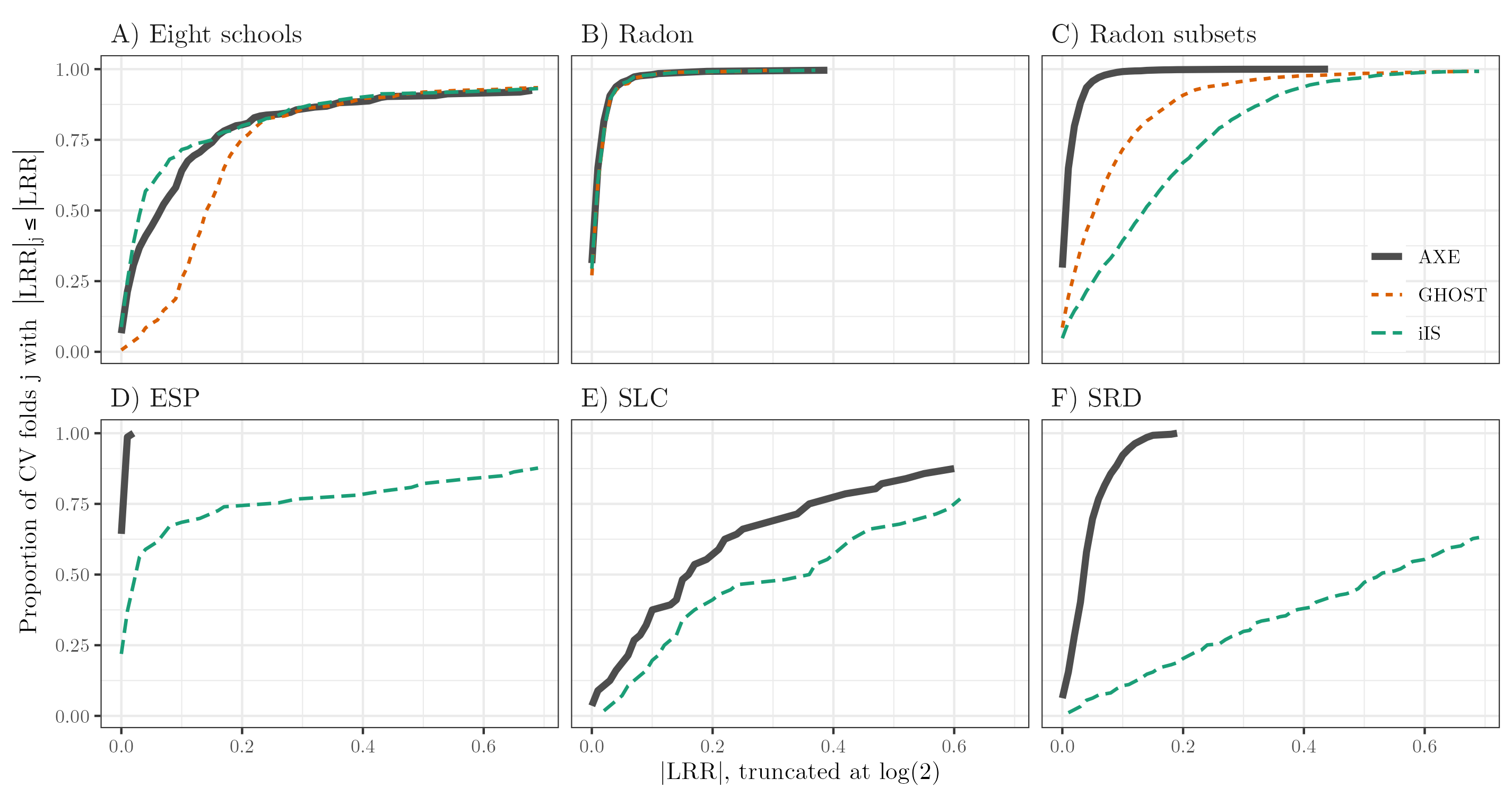
Figure 1: Line plots of the proportion of CV folds $j$ with $|\text{LRR}|_{j}\leq x$, for $x\in[0,\log(2)]$ on the x-axis. We refer to each line as an LRR percentage curve. Curves are colored and shaped based on the method used and are truncated at $\log(2)\approx 0.7$. Ghost is only applicable to LMMs in examples A, B and C.

Figure 1A shows an example where $n_{j}=1$ and LCO-CV is the same as LOO-CV. AXE and both iIS methods outperform all others, with roughly 70% of $|\text{LRR}|\leq 0.1$ compared to GHOST’s 25%. As GHOST assumes $f(\beta_{/\theta}|Y)=f(\beta_{/\theta}|Y_{-\mathpzc{s}_{j}})$, the Ghost mean estimate for this example is $\bar{Y}$, resulting in larger LRRs, while AXE and the iIS methods have mean estimate $\bar{Y}_{-\mathpzc{s}_{j}}$ (see, e.g., Eight schools in Figure 2B).

Figure 1B contains results for the full Radon data, which is a relatively rich data set compared to the number of parameters to estimate. As such, AXE, iIS, and GHOST all have over $97$% of $|\text{LRR}|$s under $0.1$. A few CV folds do have relatively large $|\text{LRR}|$; these correspond to the same two CV folds across all LCO methods and are cases where the data are particularly informative for the random effect variance.

Figure 1C contains results for the Radon subsets data, where AXE is the best-performing method with over $99$% of $|\text{LRR}|\text{s}\leq 0.1$. GHOST and iIS perform worse, with $71$% and $39$% of $|\text{LRR}|\text{s}\leq 0.1$, respectively. Each of those three methods assumes $f(\beta_{/\theta}|Y)$ and $f(\beta_{/\theta}|Y_{-\mathpzc{s}_{j}})$ are similar, but the low number of clusters in the training data means that estimation of the fixed effect coefficient for log uranium, which is a county-level estimate, can be quite different under cross-validation. We also note that in a closer examination of these results, we found that GHOST tended to underestimate RMSE for the Radon subsets data, while iIS overestimated RMSE. As GHOST uses the full-data posteriors directly, it follows that it produces over-optimistic results.

In Figure 1D, iIS is able to produce stable estimates because it incorporates information from $\beta_{/\theta}|Y$, but it is outperformed by AXE which has a nearly perfect LRR percentage curve. The good performance of AXE suggests that posterior expectations for $\beta_{/\theta}$ and $\Sigma$ were relatively stable across CV folds. In panel E, LRRs are in general larger for all methods than preceding panels (see Table LABEL:tab:lrrtable, in Appendix LABEL:appx:lrrs). This is partly due to small sample sizes, where many districts have lip cancer counts under 5, so the normal approximation is less accurate. In panel F, AXE yields satisfactory results with $92$% of $|\text{LRR}|\text{s}\leq 0.1$ while the remaining LCO approximation methods perform poorly.

We summarize each method’s performance using the area under the LRR percentage curves (AUC-LRRP) of Figure 1. An ideal method would have AUC-LRRP of $\log(2)$, and a method with all $|\text{LRR}|$s $>\log(2)$ would have AUC-LRRP of 0. We normalize AUC-LRRP and divide its value by $\log(2)$ so that the maximum is 1 and the minimum is 0. Table 4 gives AUC-LRRP$/\log(2)$ for each method and example. Further summary metrics for each method and example, consisting of mean LRR and the standard deviation of LRR, are provided in Appendix LABEL:appx:lrrs.

Table 4: Area under the LRR percentage curves of Figure 1, normalized by $\log(2)$ to have a maximum of 1. Methods with highest AUC-LRRP are bolded.

	AXE	GHOST	Vehtari	iIS	IJ-C	IJ-A	NS-C	NS-A
A) Eight schools	0.80	0.72	0.16	0.82	0.17	0.27	0.12	0.11
B) Radon	0.98	0.98	0.65	0.98	0.70	0.88	0.71	0.47
C) Radon subsets	0.98	0.88	0.83	0.76	0.82	0.56	0.53	0.32
D) ESP	1.00	**	0.92	0.76	0.10	0.71	0.17	0.26
E) SLC	0.67	**	0.35	0.52	**	**	0.19	0.34
F) SRD	0.94	**	*	0.33	**	**	0.12	0.09
* Excluded due to computation time.
** Method does not apply.

Table 4 shows that AXE most frequently has the highest AUC-LRRP, except for Eight schools where it had the second highest. The main weakness of Vehtari and iIS is the computational expense. They are the most expensive of all the methods and, in some of our examples, require more time than manual cross-validation, as discussed in Section 4.3.

Both NS and IJ performed worse than the majority of other CV approximation methods. We note that our examples have fewer observations in comparison to the number of model parameters than is typical for NS or IJ, which is usually applied to data large enough such that cross-validation using standard optimization methods is prohibitively expensive. In such situations, the large amount of data typically means that posterior densities are very narrow and $f(\beta_{/\theta},\Sigma,\phi|Y)$ is more similar to $f(\beta_{/\theta},\Sigma,\phi|Y_{-\mathpzc{s}_{j}})$. When there are fewer observations and, subsequently, more uncertainty in the model, a small change in $w$ can result in a larger change in the log-likelihood. Both methods are often limited to LOO-CV, as in Wang et al. (2018); Rad and Maleki (2020); Giordano et al. (2019) and Stephenson and Broderick (2020), which typically results in smaller changes to the log-likelihood over CV folds. We note that all of the CV approximation methods included in this paper improve as the amount of data increases; the main advantage for IJ and NS is that their computing times may scale more easily to LOO-CV with large data sets.

4.2 Point-by-point comparisons

We provide graphical point-by-point comparisons of $\hat{Y}^{(\text{method})}$ to ground-truth cross-validated $\hat{Y}^{(\text{MCV})}$. Figure 2A contains scatter plots of the AXE approximation for each data point $\hat{Y}$ against actual MCV values for all examples. The vast majority of points lie on or near the 45-degree line. In many cases, the AXE approximation is point-by-point equivalent to MCV estimates. It is in contrast to the scatter plots in Figure 2B, which contain AXE approximations as well as GHOST and iIS, both of which performed relatively well, based on Figure 1. iIS has a higher variance than AXE for the Radon subsets, ESP, and SRD data sets, with approximations farther from the 45-degree line. GHOST has a higher variance in the Eight schools and Radon subsets data sets. All three methods perform similarly in the Radon data sets.

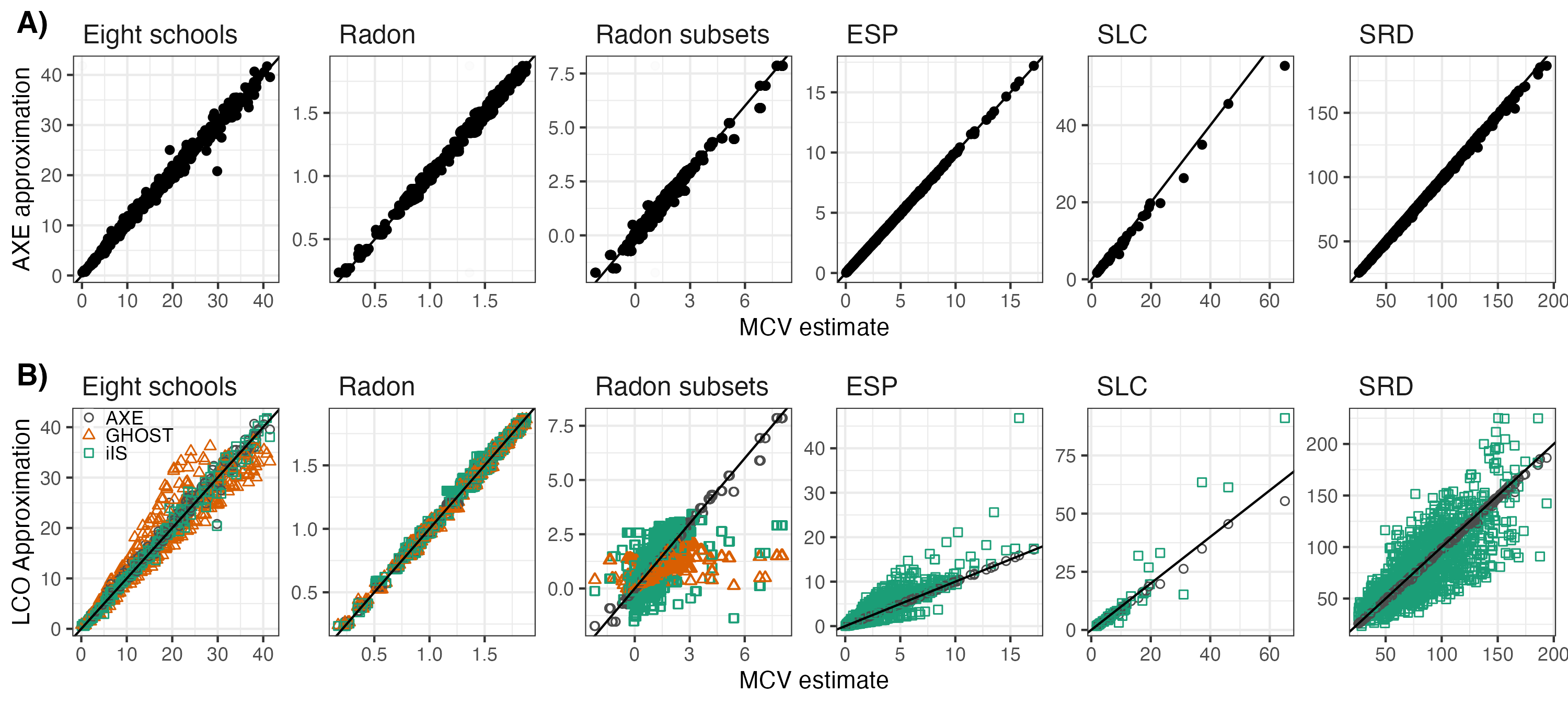
Figure 2: Scatter plots comparing the LCO approximation to ground-truth MCV estimate for each data point, model, and data set. Panels in row A compare the AXE approximation $\hat{Y}_{ji}^{\text{AXE}}$ against the MCV estimate for $E[Y_{ji}|Y_{-\mathpzc{s}_{j}}]$. Panels in row B add points with GHOST (pink triangle) and iIS (green square) approximations whenever applicable, along with AXE (black circle). Each point in a grid represents one point in the corresponding data set(s) and model(s).

We found that the accuracy of AXE was not particularly impacted as the proportion of test data increased, but it improved greatly as the number of clusters increased. For instance, some of the largest deviations from the 45-degree line are in row B, the Radon subsets data, where the number of clusters ranges from 3 to 12. It is intuitive, as the estimation of $\Sigma$ depends largely on cluster-specific intercepts, so when there are fewer clusters, $E[\Sigma|Y_{-\mathpzc{s}_{j}}]$ is less stable across CV folds.

4.3 Computation time

Table 5 provides the total computation time on an Intel i7-8700k CPU with 40 Gb of memory, to aid with running examples in parallel; note a standard 8 Gb of memory would be sufficient for the examples. Except for the SRD data, models were fit using STAN or the rstanarm package, with four chains of 2000 samples and a 1000-sample burn-in, resulting in 4000 total samples. For the SRD data, the CAR.ar() function from the CARBayesST package was used, for four chains of 220,000 samples each, with a 20,000 sample burn-in and thinned to produce 4000 total posterior samples. Calculations for IJ were conducted in Python using the autograd package. AXE took a reasonable amount of time for all examples: a few seconds for Eight schools, Radon, Radon subsets, and SLC, about one minute for ESP, and 10 minutes for SRD. To date, Vehtari has been used only in the LOO-CV case (Vehtari et al., 2016; Vanhatalo et al., 2013). When CV folds contained multiple data points, Vehtari took much longer than other approximation methods.

Table 5: Total computing time for each method in seconds, excluding time to fit the full data. Times with “h” are in hours. Times to fit the model to the full data are included for comparison.

data	AXE	GHOST	Vehtari	iIS	IJ-C	IJ-A	NS-C	NS-A	MCV
A) Eight schools	0.7	1.5	1.3h	0.6h	0.8	0.3	4.1	1.2	0.3h
B) Radon	9.1	0.5	14.5h	476.8	2.0	0.1	100.5	2.1	1.1h
C) Radon subsets	1.3	90.4	6.2h	3.6h	118.1	45.7	82.7	34.3	15.7h
D) ESP	67.7	**	55.9h	570.0	3.1	1.5	120.5	59.2	4.4h
E) SLC	0.1	**	2.8h	738.2	**	**	16.6	1.4	693.8
F) SRD	624.6	**	*	126.0h	**	**	24.5h	13.5h	40.6h
*: Method excluded due to computation time. **: Method does not apply.

5 Discussion

AXE is a fast and stable approximation method for obtaining cross-validated mean estimates. AXE is equivalent to a Frequentist cross-validation, but using the posterior means $\hat{\Sigma}$ and $\hat{\phi}$ as plug-in estimates and benefits from any subsequent computational advances. In addition to linear models, the proposed approximation is applicable to all generalized linear models that use an iterative weighted least square algorithm (IWLS). However, the accuracy of the approximation will also depend on the accuracy of IWLS. We show that AXE is more accurate when the number of CV folds is large, which is also when it saves the most time. When variance parameters are not well-estimated, we recommend an approximation diagnosis that runs MCV for a small sample of folds and checks whether the mean and standard deviation of LRRs are low.

Our empirical results show that AXE consistently performed better than more computationally expensive LCO methods. It is because AXE relies on weaker assumptions than many competing methods, making it more robust. Ghosting estimates often had absolute LRR $>0.25$ when 1) the test data were critical for estimating $\beta_{/\theta}$ and $E[\beta_{/\theta}|Y]\neq E[\beta_{/\theta}|Y_{-\mathpzc{s}_{j}}]$ or 2) the $\theta_{j}$ were not i.i.d., with $E[\theta_{j}|\theta_{-j},\Sigma]\neq 0$. The latter scenario is also when ghosting may be more computationally expensive than MCV if the test data size $n_{j}>1$. Importance sampling methods typically required longer computation times than either ghosting or AXE. They performed worse when training data posterior densities differed from the full data posterior densities, resulting in high variance. Although importance sampling has weaker assumptions than ghosting, it may also have higher variance, and there are multiple instances where ghosting outperforms importance sampling in our examples. IJ and NS were fast but consistently performed worse than other methods. In addition, IJ only applies to models where the $Y_{i}$ are conditionally independent, or $\theta$ are discrete and finite and thus could not be applied to the SLC and SRD examples in this paper.

Another category of LCO-CV approximation methods for Bayesian models in the literature is called integrated or marginal information criteria. The most notable method is the integrated Watanabe-Akaike Information Criterion (Li et al., 2016; Merkle et al., 2019). Integrated information criteria are used to approximate the expected log predictive density (ELPD), $\sum_{j=1}^{J}\log f(Y_{\mathpzc{s}_{j}}|Y_{-\mathpzc{s}_{j}})$. They do not produce estimates for $E[Y_{\mathpzc{s}_{j}}|Y_{-\mathpzc{s}_{j}}]$ and so are omitted from the CV comparisons here.

References

- Arlot et al. (2010) Arlot, S., A. Celisse, et al. (2010). A survey of cross-validation procedures for model selection. Statistics Surveys 4, 40–79.
- Bardenet et al. (2017) Bardenet, R., A. Doucet, and C. Holmes (2017). On Markov Chain Monte Carlo methods for tall data. The Journal of Machine Learning Research 18(1), 1515–1557.
- Beirami et al. (2017) Beirami, A., M. Razaviyayn, S. Shahrampour, and V. Tarokh (2017). On optimal generalizability in parametric learning. In I. Guyon, U. V. Luxburg, S. Bengio, H. Wallach, R. Fergus, S. Vishwanathan, and R. Garnett (Eds.), Advances in Neural Information Processing Systems, Volume 30. Curran Associates, Inc.
- Breslow and Clayton (1993) Breslow, N. E. and D. G. Clayton (1993). Approximate inference in generalized linear mixed models. Journal of the American statistical Association 88(421), 9–25.
- Carpenter et al. (2017) Carpenter, B., A. Gelman, M. D. Hoffman, D. Lee, B. Goodrich, M. Betancourt, M. Brubaker, J. Guo, P. Li, and A. Riddell (2017). Stan: A probabilistic programming language. Journal of Statistical Software 76(1), 1–32.
- Gelfand (1996) Gelfand, A. E. (1996). Model determination using sampling-based methods. Markov Chain Monte Carlo in Practice, 145–161.
- Gelfand et al. (1992) Gelfand, A. E., D. K. Dey, and H. Chang (1992). Model determination using predictive distributions with implementation via sampling-based methods. Technical report, Stanford Univ. CA Dept. of Statistics.
- Gelman et al. (2006) Gelman, A. et al. (2006). Prior distributions for variance parameters in hierarchical models (comment on article by browne and draper). Bayesian Analysis 1(3), 515–534.
- Gelman and Hill (2007) Gelman, A. and J. Hill (2007). Data Analysis Using Regression and Multilevel/Hierarchical Models, Volume 1. Cambridge University Press New York, NY, USA.
- Ghosh et al. (2020) Ghosh, S., W. T. Stephenson, T. D. Nguyen, S. K. Deshpande, and T. Broderick (2020). Approximate cross-validation for structured models. arXiv preprint arXiv:2006.12669.
- Giordano et al. (2019) Giordano, R., W. Stephenson, R. Liu, M. Jordan, and T. Broderick (2019). A swiss army infinitesimal jackknife. In The 22nd International Conference on Artificial Intelligence and Statistics, pp. 1139–1147. PMLR.
- Girolami and Calderhead (2011) Girolami, M. and B. Calderhead (2011). Riemann manifold Langevin and Hamiltonian Monte Carlo methods. Journal of the Royal Statistical Society: Series B (Statistical Methodology) 73(2), 123–214.
- Goodrich et al. (2018) Goodrich, B., J. Gabry, I. Ali, and S. Brilleman (2018). rstanarm: Bayesian applied regression modeling via Stan. R package version 2(4), 1758.
- Green (1984) Green, P. J. (1984). Iteratively reweighted least squares for maximum likelihood estimation, and some robust and resistant alternatives. Journal of the Royal Statistical Society: Series B (Methodological) 46(2), 149–170.
- Harville (1977) Harville, D. A. (1977). Maximum likelihood approaches to variance component estimation and to related problems. Journal of the American statistical association 72(358), 320–338.
- Holland and Welsch (1977) Holland, P. W. and R. E. Welsch (1977). Robust regression using iteratively reweighted least-squares. Communications in Statistics-theory and Methods 6(9), 813–827.
- Jaeckel (1972) Jaeckel, L. A. (1972). The infinitesimal jackknife. Bell Telephone Laboratories.
- Kass and Steffey (1989) Kass, R. E. and D. Steffey (1989). Approximate Bayesian inference in conditionally independent hierarchical models (parametric empirical Bayes models). Journal of the American Statistical Association 84(407), 717–726.
- Kingma and Welling (2013) Kingma, D. P. and M. Welling (2013). Auto-encoding variational Bayes. arXiv preprint arXiv:1312.6114.
- Koh et al. (2019) Koh, P. W., K.-S. Ang, H. H. Teo, and P. Liang (2019). On the accuracy of influence functions for measuring group effects. In Proceedings of the 33rd International Conference on Neural Information Processing Systems, pp. 5254–5264.
- Korattikara et al. (2014) Korattikara, A., Y. Chen, and M. Welling (2014). Austerity in MCMC land: Cutting the Metropolis-Hastings budget. In International Conference on Machine Learning, pp. 181–189.
- Lee et al. (2018) Lee, D., A. Rushworth, and G. Napier (2018). Spatio-temporal areal unit modelling in r with conditional autoregressive priors using the carbayesst package. Journal of Statistical Software 84(9).
- Lewis and Raftery (1997) Lewis, S. M. and A. E. Raftery (1997). Estimating Bayes factors via posterior simulation with the Laplace—Metropolis estimator. Journal of the American Statistical Association 92(438), 648–655.
- Li et al. (2016) Li, L., S. Qiu, B. Zhang, and C. X. Feng (2016). Approximating cross-validatory predictive evaluation in Bayesian latent variable models with integrated IS and WAIC. Statistics and Computing 26(4), 881–897.
- Maclaurin et al. (2015) Maclaurin, D., D. Duvenaud, and R. P. Adams (2015). Autograd: Effortless gradients in numpy. In ICML 2015 AutoML workshop, Volume 238, pp. 5.
- Marshall and Spiegelhalter (2003) Marshall, E. and D. Spiegelhalter (2003). Approximate cross-validatory predictive checks in disease mapping models. Statistics in Medicine 22(10), 1649–1660.
- Merkle et al. (2019) Merkle, E. C., D. Furr, and S. Rabe-Hesketh (2019). Bayesian comparison of latent variable models: Conditional versus marginal likelihoods. Psychometrika 84(3), 802–829.
- Opsomer et al. (2001) Opsomer, J., Y. Wang, and Y. Yang (2001). Nonparametric regression with correlated errors. Statistical Science, 134–153.
- Owen (2013) Owen, A. B. (2013). Monte Carlo Theory, Methods and Examples.
- Polson et al. (2012) Polson, N. G., J. G. Scott, et al. (2012). On the half-Cauchy prior for a global scale parameter. Bayesian Analysis 7(4), 887–902.
- Quiroz et al. (2019) Quiroz, M., R. Kohn, M. Villani, and M.-N. Tran (2019). Speeding up MCMC by efficient data subsampling. Journal of the American Statistical Association 114(526), 831–843.
- Rad and Maleki (2020) Rad, K. R. and A. Maleki (2020). A scalable estimate of the out-of-sample prediction error via approximate leave-one-out cross-validation. Journal of the Royal Statistical Society: Series B (Statistical Methodology) 82(4), 965–996.
- Rubin (1981) Rubin, D. B. (1981). Estimation in parallel randomized experiments. Journal of Educational Statistics 6(4), 377–401.
- Rue et al. (2009) Rue, H., S. Martino, and N. Chopin (2009). Approximate Bayesian inference for latent Gaussian models by using integrated nested laplace approximations. Journal of the Royal Statistical Society: Series B (Statistical Methodology) 71(2), 319–392.
- Stephenson and Broderick (2020) Stephenson, W. and T. Broderick (2020). Approximate cross-validation in high dimensions with guarantees. In International Conference on Artificial Intelligence and Statistics, pp. 2424–2434. PMLR.
- Vanhatalo et al. (2013) Vanhatalo, J., J. Riihimäki, J. Hartikainen, P. Jylänki, V. Tolvanen, and A. Vehtari (2013). Gpstuff: Bayesian modeling with Gaussian processes. Journal of Machine Learning Research 14(Apr), 1175–1179.
- Vehtari et al. (2016) Vehtari, A., T. Mononen, V. Tolvanen, T. Sivula, and O. Winther (2016). Bayesian leave-one-out cross-validation approximations for Gaussian latent variable models. The Journal of Machine Learning Research 17(1), 3581–3618.
- Vehtari et al. (2015) Vehtari, A., D. Simpson, A. Gelman, Y. Yao, and J. Gabry (2015). Pareto smoothed importance sampling. arXiv preprint arXiv:1507.02646.
- Wang et al. (2018) Wang, S., W. Zhou, H. Lu, A. Maleki, and V. Mirrokni (2018). Approximate leave-one-out for fast parameter tuning in high dimensions. In International Conference on Machine Learning, pp. 5228–5237. PMLR.