Refining Landauer’s Stack:
Balancing Error and Dissipation When Erasing Information

Abstract

Nonequilibrium information thermodynamics determines the minimum energy dissipation to reliably erase memory under time-symmetric control protocols. We demonstrate that its bounds are tight and so show that the costs overwhelm those implied by Landauer’s energy bound on information erasure. Moreover, in the limit of perfect computation, the costs diverge. The conclusion is that time-asymmetric protocols should be developed for efficient, accurate thermodynamic computing. And, that Landauer’s Stack—the full suite of theoretically-predicted thermodynamic costs—is ready for experimental test and calibration.

I Introduction

In 1961, Landauer identified a fundamental energetic requirement to perform logically-irreversible computations on nonvolatile memory [1]. Focusing on arguably the simplest case—erasing a bit of information—he found that one must supply at least $k_{\text{B}}T\ln 2$ work energy ($\approx 10^{-21}J$ at room temperature), eventually expelling this as heat. (Here, $k_{\text{B}}$ is Boltzmann’s constant and $T$ is the temperature of the computation’s ambient environment.)

Notably, though still underappreciated, Landauer had identified a thermodynamically-reversible transformation. And so, no entropy actually need be produced—energy is not irrevocably dissipated—at least in the quasistatic, thermodynamically-reversible limit required to meet Landauer’s bound.

Landauer’s original argument appealed to equilibrium statistical mechanics. Since his time, advances in nonequilibrium thermodynamics, though, showed that his bound on the required work follows from a modern version of the Second Law of thermodynamics [2]. (And, when the physical substrate’s dynamics are taken into account, this is the information processing Second Law (IPSL) [3].) These modern laws clarified many connections between information processing and thermodynamics, such as dissipation bounds due to system-state coarse-grainings [4], nanoscale information-heat engines [5], the relation of dissipation and fluctuating currents [6], and memory design [7].

Additional scalings recently emerged between computation time, space, reliability, thermodynamic efficiency, and robustness of information storage [8, 9, 10]. In contrast to Landauer’s bound, these tradeoffs involve thermodynamically-irreversible processes, implying that entropy production and therefore true heat dissipation is generally required depending on either practicality or design goals.

In addition to these tradeoffs, it is now clear that substantial energetic costs are incurred when using logic gates and allied information-processing modules to construct a computer. Especially so, when compared to custom designing hardware to optimally implement a particular computation [11].

Taken altogether these costs constitute a veritable Landauer’s Stack of the information-energy requirements for thermodynamic computing. Figure 1 illustrates Landauer’s Stack in the light of historical trends in the thermodynamic costs of performing elementary logic operations in CMOS technology. The units there are joules dissipated per logic operation. We take Landauer’s Stack to be the overhead including Landauer’s bound ($k_{\text{B}}T\ln 2$ joules) up to the current (year 2020) energy dissipations due to information processing. Thus, the Stack is a hierarchy of energy expenditures that underlie contemporary digital computing—an arena of theoretically-predicted and as-yet unknown thermodynamic phenomena waiting detailed experimental exploration.

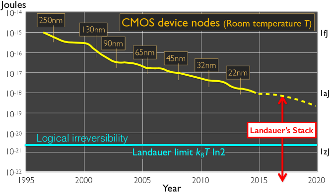
Figure 1: Historical trends in thermodynamic costs of performing elementary logic operations in CMOS technology quoted in energy dissipated (joules) per logic operation. Contemporary experimentally-accessible thermal resolution is approximately $10^{-24}$ joules. Landauer’s Stack—Thermodynamic hierarchy of predicted “overhead” energy expenditures due to information processing that underlie contemporary digital computing including Landauer’s Principle of logical irreversibility [1], now seen as a consequence of the broader information processing Second Law $\langle W\rangle\leq k_{\text{B}}T\ln\Delta h_{\mu}$ [3]: (a) Nonreciprocity [12]; (b) Computation rate $1/\tau$ [9, 10]; (c) Accuracy: $-\ln\epsilon$ [12]; (d) Storage stability; (e) Circuit modularity [11]; (f) Transitions between nonequilibrium steady-state storage states [13, 14]; and (g) Quantum coherence [15]. (2015 and prior portion of figure courtesy M. L. Roukes, data compiled from [16, and citations therein]. Landauer’s Stack cf. Table I in Ref. [17].) CMOS technology change to 3D device nodes around 2015 make linear feature size and its relation to energy costs largely incomparable afterwards [18, 19, 20, 21]. There are, of course, other sources of energy dissipation in CMOS such as leakage currents that arise when electrons tunnel from gate to drain through a thin gate-oxide dielectric. Thermodynamically, this source is kind of “housekeeping heat”, necessary to support the substrate’s electronic properties but not directly due to information processing.

To account for spontaneous deviations that arise in small-scale systems, the Second Laws are now most properly expressed by exact equalities on probability distributions of possible energy fluctuations. These are the fluctuation theorems [22], from which the original Laws (in fact, inequalities) can be readily recovered. Augmenting the Stack, fluctuation theorems apply directly to information processing, elucidating further thermodynamic restrictions and structure [23, 24, 25, 26].

The result is a rather more complete accounting for the energetic costs of thermodynamic computation, captured in the refined Landauer’s Stack of Fig. 1. In this spirit, here we report new bounds on the work required to compute in the very important case of computations driven externally by time-symmetric control protocols [12]. In surprising contrast to the fixed energy cost of erasure identified by Landauer, here we demonstrate that the scaling of the minimum required energy diverges as a function of accuracy and so can dominate Landauer’s Stack. This serves the main goal in the following to validate and demonstrate the tightness of Ref. [12]’s thermodynamic bounds and do so in Landauer’s original setting of information erasure.

In essence, our argument is as follows. Energy dissipation in thermodynamic transformations is strongly related to entropy production. The fluctuation theorems establish that entropy production depends on both forward and reverse dynamics. Thus, when determining bounds on dissipation in thermodynamic computing, one has to examine both when the control protocol is applied in forward and reverse. By considering time-symmetric protocols we substantially augment Landauer and Bennett’s dissipation bound on logical irreversibility [27] with dissipation due to logical nonselfinvertibility (aka nonreciprocity).

Why time-symmetric protocols? Modern digital computers are driven by sinusoidal line voltages and square-wave clock pulses—time-symmetric control signals. And so, modern digital computers obey the Ref. [12]’s error-dissipation trade-off. Moreover, the costs apply to even the most basic of computational tasks—such as bit erasure. Here, we present protocols for time-symmetrically implementing erasure in two different frameworks and demonstrate that both satisfy the new bounds. Moreover, many protocols approach the bounds quite closely, indicating that they may in be fact be broadly achievable.

After a brief review of the general theory, we begin with an analysis of erasure implemented with the simple framework of two-state rate equations, demonstrating the validity of the bound for different protocols of increasing reliability. We then expand our framework to fully simulated collections of particles erased in an underdamped Langevin double-well potential, seeing the same faithfulness to the bound for a wide variety of different erasure protocols. We conclude with a call for follow-on efforts to analyze even more efficient computing that can arise from time-asymmetric protocols.

II Dissipation In Thermodynamic Computing

Consider a universe consisting of a computing device—the system under study (SUS), a thermal environment at fixed inverse temperature $\beta$, and a laboratory device (lab) that includes a work reservoir. The set of possible microstates for the SUS is denoted $\bm{\mathcal{S}}$, with $s$ denoting an individual SUS microstate. The SUS is driven by a control parameter $x$ generated by the lab. The SUS is also in contact with the thermal environment.

The overall evolution occurs from time $t=0$ to $t=\tau$ and is determined by two components. The first is the SUS’s Hamiltonian $\mathcal{H}_{SL}(s,x)$ that specifies its interaction with the lab device and determines (part of) the rates of change of the SUS coordinates consistent with Hamiltonian mechanics. We refer to the possible values of the Hamiltonian as the SUS energies. The second component is the thermal environment which exerts a stochastic influence on the system dynamics.

We prepare the lab to guarantee that a specific control parameter value $x(t)$ is applied to the SUS at every time $t$ over the time interval $t\in(0,\tau)$. That is, the control parameter evolves deterministically as a function of time. The deterministic trajectory taken by the control parameter $x(t)$ over the computation interval is the control protocol, denoted by $\overrightarrow{x}$. The SUS microstate $s(t)$ exhibits a response to the control protocol, over the interval following a stochastic trajectory denoted $\overrightarrow{s}$.

For a given microstate trajectory $\overrightarrow{s}$, the net energy transferred from the lab to the SUS is defined as the work, which has the following form [5]:

$$W(\overrightarrow{s})=\int_{0}^{\tau}dt\,\dot{x}(t)\frac{\partial\mathcal{H}_{SL}}{\partial x}\Big{|}_{(s(t),x(t))}~{}.$$

This is the energy accumulated in the SUS directly caused by changes in the the control parameter.

Given an initial microstate $s_{0}$, the probability of a microstate trajectory $\overrightarrow{s}$ conditioned on starting in $s_{0}$ is denoted:

$$P(\overrightarrow{s}|s_{0})=\Pr_{\overrightarrow{x}}(\overrightarrow{\mathcal{S}}=\overrightarrow{s}|\mathcal{S}_{0}=s_{0})~{}.$$

With the SUS initialized in microstate distribution $\bm{\mu}_{0}$, the unconditioned forward process gives the probability of trajectory $\overrightarrow{s}$:

$$P(\overrightarrow{s})=P(\overrightarrow{s}|s(0))\bm{\mu}_{0}(s(0))~{}.$$

Detailed fluctuation theorems (DFTs) [28, 29] determine thermodynamic properties of the computation by comparing the forward process to the reverse process. This requires determining the conditional probability of trajectories under time-reversed control:

$$R(\overrightarrow{s}|s_{0})=\Pr_{\reflectbox{$\mathbf{R}$}\overrightarrow{x}}(\overrightarrow{\mathcal{S}}=\overrightarrow{s}|\mathcal{S}_{0}=s_{0})~{}.$$

The reverse control protocol is $\reflectbox{$\mathbf{R}$}x(t)=x(\tau-t)^{\dagger}$, where $x^{\dagger}$ is $x$, but with all time-odd components (e.g., magnetic field) flipped in sign. And, the reverse process results from the application of this dynamic to the final distribution $\bm{\mu}_{\tau}$ of the forward process with microstates conjugated:

$$R(\overrightarrow{s}) =R(\overrightarrow{s}|s(0))\bm{\mu}_{\tau}(s(0)^{\dagger})~{}.$$

The Crooks DFT [29] then gives an equality on both the dissipated work (or entropy production) that is produced as well as the required work for a given trajectory induced by the protocol:

$$\beta W_{\text{diss}}(\overrightarrow{s}) =\ln\frac{P(\overrightarrow{s})}{R(\reflectbox{$\mathbf{R}$}\overrightarrow{s})}.$$

$\reflectbox{$\mathbf{R}$}\overrightarrow{s}$ here is itself a SUS microstate trajectory with $\reflectbox{$\mathbf{R}$}s(t)=s(\tau-t)^{\dagger}$.

Due to their practical relevance, we consider protocols that are symmetric under time reversal $\reflectbox{$\mathbf{R}$}\overrightarrow{x}=\overrightarrow{x}$. That is, the reverse-process probability of trajectory $\overrightarrow{s}$ conditioned on starting in microstate $s_{0}$ is the same as that of the forward process:

$$R(\overrightarrow{s}|s_{0})=P(\overrightarrow{s}|s_{0})~{}.$$

However, the unconditional reverse process probability of the trajectory $\overrightarrow{s}$ is then:

$$R(\overrightarrow{s}) =P(\overrightarrow{s}|s(0))\bm{\mu}_{\tau}(s(0)^{\dagger})~{}.$$

This leads to a version of Crook’s DFT that can be used to set modified bounds on a computation’s dissipation:

$$\beta W_{\text{diss}}(\overrightarrow{s})=\ln\frac{P(\overrightarrow{s}|s(0))\bm{\mu}_{0}(s(0))}{P(\reflectbox{$\mathbf{R}$}\overrightarrow{s}|s(\tau)^{\dagger})\bm{\mu}_{\tau}(s(\tau))}~{}.$$

Suppose, now, that the final and initial SUS Hamiltonian configurations $\mathcal{H}_{SL}(s,x(\tau))$ and $\mathcal{H}_{SL}(s,x(0))$ are both designed to store the same information about the SUS. The SUS microstates are partitioned into locally-stable regions that are separated by large energy barriers in these energy landscapes. On some time scale, a state initialized in one of these regions has a very low probability of escape and instead locally equilibrates to its locally-stable region. These regions can thus be used to store information for periods of time controlled by the energy barrier heights. Collectively, we refer to these regions as memory states $\bm{\mathcal{M}}$.

Then the probability of the system evolving to a memory state $m^{\prime}\in\bm{\mathcal{M}}$ given that it starts in a memory state $m\in\bm{\mathcal{M}}$ under either the forward or reverse process is:

$$P^{\prime}(m\rightarrow m^{\prime}) =\frac{\int d\overrightarrow{s}\bigl{[}\!\!\bigl{[}s(0)\in m\land s(\tau)\in m^{\prime}\bigr{]}\!\!\bigr{]}P(\overrightarrow{s})}{\int d\overrightarrow{s}\bigl{[}\!\!\bigl{[}s(0)\in m\bigr{]}\!\!\bigr{]}P(\overrightarrow{s})}~{},$$

where $\bigl{[}\!\!\bigl{[}E\bigr{]}\!\!\bigr{]}$ evaluates to one if expression $E$ is true and zero otherwise.

Reference [12]’s Eq. (15) bounds the average entropy production derived under weaker restrictions than assumed here. Applying it and simplifying, we obtain:

$$\beta\langle W_{\text{diss}}\rangle \geq\Delta H(\mathcal{M}(t))+\!\!\sum_{m\in\bm{\mathcal{M}}}\!\!\bm{\mu}_{0}^{\prime}(m)\!\!\sum_{m^{\prime}\in\bm{\mathcal{M}}}\!\!d(m,m^{\prime}),$$ (1)

where:

$$\bm{\mu}_{0}^{\prime}(m) =\int ds\bigl{[}\!\!\bigl{[}s\in m\bigr{]}\!\!\bigr{]}\bm{\mu}_{0}(s)~{},$$

$$d(m,m^{\prime}) =P^{\prime}(m\rightarrow m^{\prime})\ln\frac{P^{\prime}(m\rightarrow m^{\prime})}{P^{\prime}(m^{\prime}\rightarrow m)}~{},$$

assuming time-reversal invariant memories, and $\Delta H(\mathcal{M}(t))$ is the change in Shannon entropy of the memory distribution.

To simplify the development, suppose that the energy landscape of each memory state looks the same locally. That is, up to translation and possibly reflection and rotation, each memory state spans the same range in microstate space and has the same energies at each of those states. Further, suppose that the SUS starts and ends in a metastable equilibrium distribution, differing from global equilibrium only in the weight that each memory state is given in the distribution. Otherwise the distribution looks identical to the global equilibrium at the local scale of any memory state. This ensures that the average change in SUS energy is zero, simplifying the average nonequilibrium free energy [12]:

$$\Delta\mathcal{F}=-\beta^{-1}\Delta H(\mathcal{M}_{t})~{}.$$

Recalling that $\beta\braket{W_{\text{diss}}(\overrightarrow{s})}=\beta(\braket{W(\overrightarrow{s})}-\Delta\mathcal{F})$ and appealing to the inequality in Eq. (1), we find a simple bound on the average work over the protocol:

$$\beta\langle W\rangle \geq\sum_{m\in\bm{\mathcal{M}}}\bm{\mu}_{0}^{\prime}(m)\sum_{m^{\prime}\in\bm{\mathcal{M}}}d(m,m^{\prime})$$ (2)

$$\equiv\beta\langle W\rangle_{\text{min}}^{\text{t-sym}}~{}.$$

This provides a bound on the work that depends solely on the logical operation of the computation, but goes beyond Landauer’s bound.

Since we are addressing modern computing, we consider processes that approximate deterministic computations on the memory states. For such computations there exists a computation function $C:\bm{\mathcal{M}}\to\bm{\mathcal{M}}$ such that the physically-implemented stochastic map approximates the desired function up to some small error. That is, $P^{\prime}(m\rightarrow C(m))=1-\epsilon_{m}$ where $0<\epsilon_{m}\ll 1$. In fact, we require all relevant errors to be bound by a small error-threshold $\epsilon\ll 0$. That is, for all $C(m)\neq m^{\prime}$, let $P^{\prime}(m,m^{\prime})=\epsilon_{{m}\to{m^{\prime}}}$ so that $0\leq\sum_{m^{\prime}\neq C(m)}\epsilon_{{m}\to{m^{\prime}}}=\epsilon_{m}\leq\epsilon\ll 1$.

We can then simplify Eq. (2)’s bound in the limit of small $\epsilon$. First, we show that $d(m,m^{\prime})\geq 0$ for any pair of $m,m^{\prime}$ in the small $\epsilon$ limit, where we have:

$$d(m,m^{\prime}) =P^{\prime}({m}\to{m^{\prime}})\ln\frac{P^{\prime}({m}\to{m^{\prime}})}{P^{\prime}({m^{\prime}}\to{m})}$$

$$\geq P^{\prime}({m}\to{m^{\prime}})\ln P^{\prime}({m}\to{m^{\prime}})~{}.$$

If $C(m)=m^{\prime}$, then $P^{\prime}({m}\to{m^{\prime}})=1-\epsilon_{m}\geq 1-\epsilon$, so that:

$$d(m,m^{\prime}) \geq(1-\epsilon)\ln(1-\epsilon)~{},$$

which vanishes as $\epsilon\to 0$. And, if $C(m)\neq m^{\prime}$, then $P^{\prime}({m}\to{m^{\prime}})=\epsilon_{{m}\to{m^{\prime}}}$, so that:

$$d(m,m^{\prime}) \geq\epsilon_{{m}\to{m^{\prime}}}\ln\epsilon_{{m}\to{m^{\prime}}}$$

which also vanishes as $\epsilon\to 0$. Setting this asymptotic lower bound on the dissipation of each transition facilitates isolating divergent contributions, such as those we now consider.

An unreciprocated memory transition $C(m)=m^{\prime}$ is one that does not map back to itself: $C(m^{\prime})\neq m$. The contribution to the dissipation bound is:

$$d(m,m^{\prime}) =(1-\epsilon_{m})\ln\frac{1-\epsilon_{m}}{\epsilon_{{m^{\prime}}\to{m}}}$$

$$\geq(1-\epsilon)\ln\frac{1-\epsilon}{\epsilon}~{}.$$

As $\epsilon\to 0$, this gives:

$$d(m,m^{\prime})\geq\ln\epsilon^{-1}~{}.$$ (3)

That is, as computational accuracy increases ($\epsilon\to 0$), $d(m,m^{\prime})$ diverges. This means the minimum-required work (Eq. (2)) must then also diverge.

We then arrive at our simplified bound for the small-$\epsilon$ high-accuracy limit from Eq. (2)’s inequality on dissipation by only including the contribution from unreciprocated transitions $m^{\prime}=C(m)$ for which $m\neq C(m^{\prime})$:

$$\beta\langle W\rangle \geq\ln(\epsilon^{-1})\sum_{m\in\bm{\mathcal{M}}}\bm{\mu}_{0}^{\prime}(m)\bigl{[}\!\!\bigl{[}C(C(m))\neq m\bigr{]}\!\!\bigr{]}$$ (4)

$$\equiv\beta\langle W\rangle_{\text{min}}^{\text{approx}}~{}.$$

In this way, we see how computational accuracy drives a thermodynamic cost that diverges, overwhelming the Landauer-erasure cost.

To be quantitative beyond a formal divergence, consider contemporary DRAM memory which exhibits a range of “soft” error rates around $10^{-22}$ failures per write operation [30]. In fact, each write operation is effectively an erasure. (The quoted statistic is an average of $4,000$ correctable errors per $128$ MB DIMM per year.) This gives a thermodynamic cost of $66~{}k_{\text{B}}T$, which is markedly larger than Landauer’s $k_{\text{B}}T\ln 2$ factor. It is also, just as clearly, smaller by a factor of roughly $10^{3}$ than the contemporary energy costs per logic operation displayed in Fig. 1. These comparisons are harbingers of the substantial effort that lies ahead to fully flesh-out and fairly calibrate costs in Landauer’s Stack.

III Erasure Thermodynamics

Inequalities Eqs. (2) and (4) place severe constraints on the work required to process information via time-symmetric control on memories. The question remains, though, whether or not these bounds can actually be met by specific protocols or if there might be still tighter bounds to be discovered.

To help answer this question, we turn to the case, originally highlighted by Landauer [1], of erasing a single bit of information. This remarkably simple case of computing has held disproportionate sway in the development of thermodynamic computing compared to other elementary operations. The following does not deviate from this habit, showing, in fact, that there remain fundamental issues. We explore this via two different implementations. The first, described via two-state rate equations and the second with an underdamped double-well potential—Landauer’s original, preferred setting.

Suppose the SUS supports two (mesoscopic) memory states, labeled L and R. The task of a time-symmetric protocol that implements erasure is to guide the SUS microscopic dynamics that starts with an initial $50-50$ distribution over the two memory states to a final distribution as biased as possible onto the L state. The logical function $C$ of perfect bit erasure is attained when $C(\text{L})=C(\text{R})=\text{L}$, setting either memory state to L. The probabilities of incorrectly sending an L state to R and an R state to R are denoted $\epsilon_{\text{L}}$ and $\epsilon_{\text{R}}$, respectively.

Error generation is described by the binary asymmetric channel [31]—the erasure channel $\mathcal{E}$ with conditional probabilities:

$$\mathcal{E}=\hbox{}\vbox{\kern 0.86108pt\hbox{$\kern 0.0pt\kern 2.5pt\kern-5.0pt\left(\kern 0.0pt\kern-2.5pt\kern-6.66669pt\vbox{\kern-0.86108pt\vbox{\vbox{ \halign{\kern\arraycolsep\hfil\@arstrut$\kbcolstyle#$\hfil\kern\arraycolsep& \kern\arraycolsep\hfil$\@kbrowstyle#$\ifkbalignright\relax\else\hfil\fi\kern\arraycolsep&& \kern\arraycolsep\hfil$\@kbrowstyle#$\ifkbalignright\relax\else\hfil\fi\kern\arraycolsep\cr 5.0pt\hfil\@arstrut$\scriptstyle$\hfil\kern 5.0pt&5.0pt\hfil$\scriptstyle\mathcal{M}_{\tau}=\text{L}$\hfil\kern 5.0pt&5.0pt\hfil$\scriptstyle\mathcal{M}_{\tau}=\text{R}\\\mathcal{M}_{0}=\text{L}$\hfil\kern 5.0pt&5.0pt\hfil$\scriptstyle 1-\epsilon_{\text{L}}$\hfil\kern 5.0pt&5.0pt\hfil$\scriptstyle\epsilon_{\text{L}}\\\mathcal{M}_{0}=\text{R}$\hfil\kern 5.0pt&5.0pt\hfil$\scriptstyle\epsilon_{\text{R}}$\hfil\kern 5.0pt&5.0pt\hfil$\scriptstyle 1-\epsilon_{\text{R}}$\hfil\kern 5.0pt\crcr}}}}\right)$}}~{}.$$

For any erasure implementation, this Markov transition matrix gives the error rate $\epsilon_{\text{L}}=\epsilon_{\text{L}\rightarrow\text{R}}$ from initial memory state $\mathcal{M}_{0}=\text{L}$ and the error rate $\epsilon_{\text{R}}=\epsilon_{\text{R}\rightarrow\text{R}}$ from the initial memory state $\mathcal{M}_{0}=\text{R}$.

Noting first that $d(m,m)=0$ generically, we then have:

$$d(\text{L},\text{R}) =\epsilon_{\text{L}}\ln\frac{\epsilon_{\text{L}}}{1-\epsilon_{\text{R}}}~{},$$

$$d(\text{R},\text{L}) =(1-\epsilon_{\text{R}})\ln\frac{1-\epsilon_{\text{R}}}{\epsilon_{\text{L}}}~{}.$$

So, the bound of Eq. (2) simplifies to:

$$\beta\langle W\rangle_{\text{min}}^{\text{t-sym}} =\frac{1}{2}\epsilon_{\text{L}}\ln\frac{\epsilon_{\text{L}}}{1-\epsilon_{\text{R}}}+\frac{1}{2}(1-\epsilon_{\text{R}})\ln\frac{1-\epsilon_{\text{R}}}{\epsilon_{\text{L}}}$$

$$=\Big{(}\frac{1}{2}-\langle\epsilon\rangle\Big{)}\ln\frac{1-\epsilon_{\text{R}}}{\epsilon_{\text{L}}}~{},$$ (5)

where $\langle\epsilon\rangle=(\epsilon_{\text{L}}+\epsilon_{\text{R}})/2$ is the average error for the process.

Notice further that $C(C(\text{L}))=\text{L}$ but $C(C(\text{R}))\neq\text{R}$, indicating that only the computation on R is nonreciprocal. Therefore, the bound of Eq. (4) simplifies to

$$\beta\langle W\rangle_{\text{min}}^{\text{approx}} =\frac{1}{2}\ln(\epsilon^{-1})~{}.$$ (6)

III.1 Erasure with Two-state Rate Equations

A direct test of time-symmetric erasure requires only a simple two-state system that evolves under a rate equation:

$$\frac{d\Pr(\mathcal{M}_{t}=m)}{dt}$$ (7)

$$=\sum_{m^{\prime}}\big{[}r_{m^{\prime}\rightarrow m}(t)\Pr(\mathcal{M}_{t}=m^{\prime})-r_{m\rightarrow m^{\prime}}(t)\Pr(\mathcal{M}_{t}=m)\big{]},$$

obeying the Arrhenius equations:

$$r_{\text{R}\rightarrow\text{L}}(t) =Ae^{-\Delta E_{\text{R}}(t)/k_{\text{B}}T}~{}\text{and}$$

$$r_{\text{L}\rightarrow\text{R}}(t) =Ae^{-\Delta E_{\text{L}}(t)/k_{\text{B}}T}~{},$$

where the states are labeled $\{\text{L},\text{R}\}$ and the terms $\Delta E_{\text{R}}(t)$ and $\Delta E_{\text{L}}(t)$ in the exponentials are the activation energies to transit over the energy barrier at time $t$ for the Right and Left wells, respectively.

These dynamics are a coarse-graining of thermal motion in a double-well potential energy landscape $V(q,t)$ over the positional variable $q$ at time $t$. Above, $A$ is an arbitrary constant, which is fixed for the dynamics. $q^{*}_{\text{R}}$ and $q^{*}_{\text{L}}$ are the locations of the Right and Left potential well minima, respectively. Thus, assuming that $q=0$ is the location of the barrier’s maximum between them, we see that the activation energies can be expressed as $\Delta E_{\text{R}}(t)=V(0,t)-V(q^{*}_{\text{R}},t)$ and $\Delta E_{\text{L}}(t)=V(0,t)-V(q^{*}_{\text{L}},t)$. By varying the potential energy extrema $V(q^{*}_{\text{R}},t)$, $V(q^{*}_{\text{L}},t)$, and $V(0,t)$ we control the dynamics of the observed variables $\{\text{L},\text{R}\}$ in much the same way as is done with physical implementations of erasure where barrier height and tilt are controlled in a double-well [32].

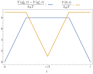
Figure 2: Time-symmetric control protocol for implementing moderately-efficient erasure. This should be compared to Landauer’s original time-symmetric protocol [1]. It starts by tilting—increasing the difference in potential energy $(V(q^{*}_{\text{R}},t)-V(q^{*}_{\text{L}},t))/k_{\text{B}}T$ between L and R. We increase this value such that transitions are more likely to go from R to L. Then we reduce the barrier height $V(0,t)$ to increase the total flow rate. Finally, we reverse the previous steps, cutting off the flow by raising the barrier, then untilting.

Deviating from previous investigations of efficient erasure, where Landauer’s bound was nearly achieved over long times [32, 33], here the constraint to symmetric driving over the interval $t\in(0,\tau)$ results in additional dissipated work. As Landauer described [1], erasure can be implemented by turning on and off a tilt from R to L—a time symmetric protocol. However, to achieve higher accuracy, we also lower the barrier while the system is tilted energetically towards the L well.

Consider a family of control protocols that fit the profile shown in Fig. 2. First, we increase the energy tilt from R to L via the energy difference $V(q^{*}_{\text{R}},t)-V(q^{*}_{\text{L}},t)$ measured in units of $k_{\text{B}}T$. This increases the relative probability of transitioning R to L. However, with the energy barrier at it’s maximum height, the transition takes quite some time. Thus, we reduce the energy barrier $V(0,t)$ to its minimum height halfway through the protocol $t=\tau/2$. Then, we reverse the protocol, raising the barrier back to its default height to hold the probability distribution fixed in the well and untilt so that the system resets to its default double-well potential.

Increasing the maximum tilt—given by $V(q^{*}_{\text{R}},\tau/2)-V(q^{*}_{\text{L}},\tau/2)$ at the halfway time—increases erasure accuracy. Figure 3 shows that the maximum error $\epsilon=\max\{\epsilon_{\text{R}},\epsilon_{\text{L}}\}$ decreases nearly exponentially with increased maximum energy difference between left and right, going below $1$ error in every $1000$ trials for our parameter range. Note that $\epsilon$ starts at a very high value (greater than $1/2$) for zero tilt, since the probability $\epsilon_{\text{R}}=\epsilon$ of ending in the R well starting in the R well is very high if there is no tilt to push the system out of the R well.

Figure 3 also shows the relationship between the work and the bounds described above. Given that our system consists of two states $\{\text{L},\text{R}\}$ and that we choose a control protocol that keeps the energy on the left $V(q^{*}_{\text{L}},t)$ fixed, the work (marked by green $+$s in the figure) is [5]:

$$\langle W\rangle =\int_{0}^{\tau}dt\sum_{s}\Pr(\mathcal{S}_{t}=s)\partial_{t}V(s,t)$$

$$=\int_{0}^{\tau}dt\Pr(\mathcal{M}_{t}=\text{R})\partial_{t}V(q^{*}_{\text{R}},t)~{}.$$

This work increases almost linearly as the error reduces exponentially.

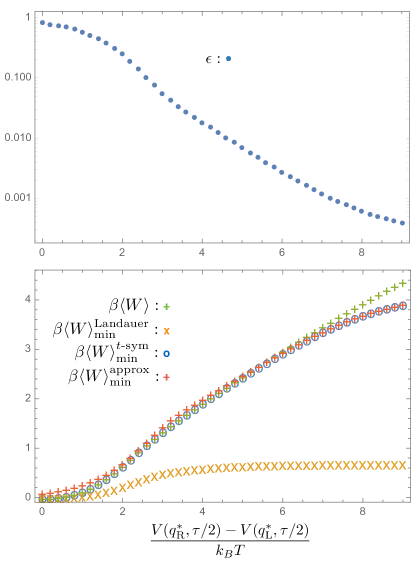
Figure 3: (Top) Maximum error $\epsilon$ (blue dots) decreases approximately exponentially with increasing maximum tilt. The latter is given by the maximum energy difference between the right and left energy well $V(q^{*}_{\text{R}},\tau/2)-V(q^{*}_{\text{L}},\tau/2)$. (Bottom) Work $\langle W\rangle$ (green $+$s), scaled by the inverse temperature $\beta=1/k_{\text{B}}T$, increases with increasing maximum tilt and decreasing error. The Landauer work bound $\braket{W}^{\text{Landauer}}_{\text{min}}$ (orange $\times$s) is a very weak bound, asymptoting to a constant value rather than continuing to increase, as the work does. The bound $\langle W\rangle^{t\text{-sym}}_{\text{min}}$ (blue circles) on time-symmetrically driven protocols, on the other hand, is a very tight bound for lower values of maximum tilt. The work deviates from the time-symmetric bound for higher tilts. Finally, the approximate bound $\braket{W}_{\text{min}}^{\text{approx}}$ (red $+$s), which scales as $\ln\epsilon^{-1}$, is not an accurate bound over the entire range, but it very closely matches the exact time-symmetric bound $\langle W\rangle^{t\text{-sym}}_{\text{min}}$ for small $\epsilon$, as expected.

As a first comparison, note that the Landauer bound $\langle W\rangle^{\text{Landauer}}_{\text{min}}=-k_{\text{B}}T\Delta H(\mathcal{M}_{t})$ (marked by orange $\times$s in the figure) is still valid. However, it is a very weak bound for this time-symmetric protocol. The Landauer bound saturates at $k_{\text{B}}T\ln 2$. Thus, the dissipated work—the gap between orange $\times$s and green $+$s—grows approximately linearly with increasing tilt energy.

In contrast, Eq. (5)’s bound $\langle W\rangle_{\text{min}}^{t\text{-sym}}$ for time symmetric protocols is much tighter. The time symmetric bound is valid: marked by blue circles that all fall below the calculated work (green $+$s). Not only is this bound much stricter, but it almost exactly matches the calculated work for a large range of parameters, with the work only diverging for higher tilts and lower error rates.

Finally, the approximate bound $\langle W\rangle_{\text{min}}^{\text{approx}}=\frac{k_{\text{B}}T}{2}\ln\epsilon^{-1}$ (marked by red $+$s) of Eq. (6), which captures the error scaling, behaves as expected. The error-dependent work bound nearly exactly matches the exact bound for low error rates on the right side of the plot and effectively bounds the work. For lower tilts, this quantity does not bound the work and is not a good estimate of the true bound, but this is consistent with expectations for high error rates. This approximation should only be employed for very reliable computations, for which it appears to be an excellent estimate. Thus, the two-level model of erasure demonstrates that the time-symmetric control bounds on work and dissipation are reasonable in both their exact and approximate forms at low error rates.

III.2 Erasure with an Underdamped Double-well Potential

The physics in the rate equations above represents a simple model of a bistable thermodynamic system, which can serve as an approximation for many different bistable systems. One possible interpretation is a coarse-graining of the Langevin dynamics of a particle moving in a double-well potential. To explore the broader validity of the error–dissipation tradeoff, here we simulate the dynamics of a stochastic particle coupled to a thermal environment at constant temperature and a work reservoir via such a 1D potential. Again, we find that the time-symmetric bounds are much tighter than Landauer’s, reflecting the error–dissipation tradeoff of this control protocol class.

Consider a one-dimensional particle with position and momentum in an external potential and in thermal contact with the environment at temperature $T$. We consider a protocol architecture similar to that of Sec. III.1, but with additional passive substages at the beginning middle and end: (i) hold the potential in the symmetric double-well form, (ii) positively tilt the potential, (iii) completely drop the potential barrier between the two wells, (iv) hold the potential while it is tilted with no barrier, (v) restore the original barrier, (vi) remove the positive tilt, restoring the original symmetric double-well, and (vii) hold the potential in this original form.

As a function of position $q$ and time $t$, the potential then takes the form:

$$V(q,t)=aq^{4}-b_{0}b_{f}(t)q^{2}+c_{0}c_{f}(t)q~{},$$

with constants $a,b_{0},c_{0}>0$. The protocol functions $b_{f}(t)$ and $c_{f}(t)$ evolve in a piecewise linear, cyclic, and time-symmetric manner according to Table 1, where $t_{0},t_{1},\ldots,t_{7}=0,\tau/12,3\tau/12,5\tau/12,7\tau/12,9\tau/12,11\tau/12,\tau$. The potential thus begins and ends in a symmetric double-well configuration with each well defining a memory state. During the protocol, though, the number of metastable regions is temporarily reduced to one. Figure 4 (top three panels) shows the protocol functions over time as well as the resultant potential function at key times for one such set of protocol parameters; see nondimensionalization in App. A. At any time, we label the metastable regions from most negative position to most positive the L state and, if it exists, the R state.

$t$	$t_{0}$		$t_{1}$		$t_{2}$		$t_{3}$		$t_{4}$		$t_{5}$		$t_{6}$		$t_{7}$
$b_{f}(t)$	$\biggr{|}$	1	$\biggr{|}$	1	$\biggr{|}$	$\frac{t_{3}-t}{t_{3}-t_{2}}$	$\biggr{|}$	0	$\biggr{|}$	$\frac{t-t_{4}}{t_{5}-t_{4}}$	$\biggr{|}$	$1$	$\biggr{|}$	$1$	$\biggr{|}$
$c_{f}(t)$	$\biggr{|}$	0	$\biggr{|}$	$\frac{t-t_{1}}{t_{2}-t_{1}}$	$\biggr{|}$	1	$\biggr{|}$	$1$	$\biggr{|}$	$1$	$\biggr{|}$	$\frac{t_{6}-t}{t_{6}-t_{5}}$	$\biggr{|}$	$0$	$\biggr{|}$

Table 1: Erasure protocol.

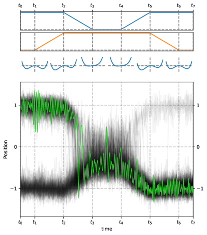
Figure 4: Erasure via an underdamped double-well potential: Protocol functions $b(t)$ (top panel, blue) and $c(t)$ (second panel, orange) are symmetric in time, guaranteeing the potential function (third panel) to evolve symmetrically in time. Due to the spatial asymmetry in the potential over the majority of the protocol, however, erasure to state L ($x<0$) typically occurs, evidenced by the evolution of the system position for $100$ randomly-chosen trajectories (bottom panel, black). The L and R states merge into one between times $t_{2}$ and $t_{3}$ and separate again between times $t_{4}$ and $t_{5}$. A single trajectory (bottom panel, green) shows the typical behavior of falling into the $x<0$ region by time $t_{3}$ and remaining there when the L state is reintroduced for the rest of the protocol.

We simulate the motion of the particle with underdamped Langevin dynamics:

$$dq =vdt$$

$$mdv =-\left(\frac{\partial}{\partial q}V(q,t)+\lambda v\right)dt+\sqrt{2k_{\text{B}}T\lambda}\,r(t)\sqrt{dt}~{},$$

where $k_{\text{B}}$ is Boltzmann’s constant, $\lambda$ is the coupling between the thermal environment and particle, $m$ is the particle’s mass, and $r(t)$ is a memoryless Gaussian random variable with $\langle r(t)\rangle=0$ and $\langle r(t)r(t^{\prime})\rangle=\delta(t-t^{\prime})$. The particle is initialized to be in global equilibrium over the initial potential $V(\cdot,0)$. Figure 4 (bottom panel) shows $100$ randomly-chosen resultant trajectories for a choice of process parameters.

The work done on a single particle over the course of the protocol with trajectory $\{q(t)\}_{t}$ is [5]:

$$W=\int_{0}^{\tau}dt\frac{\partial V(q,t)}{\partial t}\Big{|}_{q=q(t)}~{}.$$

Figure 5 shows the net average work over time for an erasure process, comparing it to (i) the Landauer bound, (ii) the exact bound of Eq. (5), and (iii) the approximate bound of Eq. (6). Notice that the final net average work lies above all three, as it should and that the time-symmetric bounds presented here are tighter than Landauer’s.

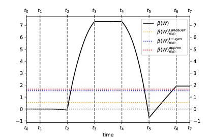
Figure 5: Average work in $k_{\text{B}}T$ over time for an erasure (black). Calculated from the simulation-estimated values $\epsilon_{L}$ and $\epsilon_{R}$, Landauer’s bound is given by the dashed yellow line and our approximate and exact bounds (Eqs. (6) and (5)) are given in dashed red and blue lines, respectively.

We repeat this comparison for an array of different parameters for the erasure protocol. As described in App. A, we vary features of the dynamics—including mass $m$, temperature $T$, coupling to the heat bath $\lambda$, duration of control $\tau$, maximum depth of the potential energy wells, and maximum tilt between the wells. Nondimensionalization reduces the relevant parameters to just four, allowing us to explore a broad swathe of possible physical erasures with 735 different protocols. For each protocol, we simulate 100,000 trajectories to estimate the work cost and errors $\epsilon_{\text{R}}$ and $\epsilon_{\text{L}}$ of the operation.

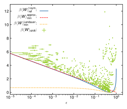
Figure 6: Reference bound $\langle W\rangle_{\text{ref}}^{t\text{-sym}}$ (blue line) lower bounds all of the shifted works $\langle W\rangle_{\text{shift}}$ (green markers), often quite tightly. The approximate bound $\langle W\rangle_{\text{min}}^{\text{approx}}$ (red dashed line) rapidly converges with decreasing error to $\langle W\rangle_{\text{ref}}^{t\text{-sym}}$. Time-asymmetric protocols can do better, needing only to satisfy Landauer’s bound $\langle W\rangle_{\text{min}}^{\text{Landauer}}$ (orange dotted line).

Figure 6 compares the work spent for each of the 735 erasure protocols to the sampled maximum error $\epsilon=\max(\epsilon_{\text{L}},\epsilon_{\text{R}})$. Each protocol corresponds to a green cross, whose vertical position corresponds to the shifted work $\langle W\rangle_{\text{shift}}$, which accounts for inhomogeneities in the error rate. Note that the exact bound $\langle W\rangle_{\text{min}}^{t\text{-sym}}$ from Eq. (5) reduces to a simple relationship between work and error tolerance $\epsilon$ when the errors are homogeneous $\epsilon_{\text{R}}=\epsilon_{\text{L}}=\epsilon$:

$$\langle W\rangle^{t\text{-sym}}_{\text{ref}}=\left(\frac{1}{2}-\epsilon\right)\ln\frac{1-\epsilon}{\epsilon}~{},$$

which we plot with the blue curve in Fig. 6. The cost of inhomogeneities in the error is evaluated by the difference between this reference bound and the exact work bound. This cost is added to the calculated work for each protocol to determine the shifted work:

$$\langle W\rangle_{\text{shift}}=\langle W\rangle+\langle W\rangle^{t\text{-sym}}_{\text{ref}}-\langle W\rangle^{t\text{-sym}}_{\text{min}}~{},$$

such that the vertical distance between $\langle W\rangle_{\text{shift}}$ and $\langle W\rangle_{\text{ref}}^{t\text{-sym}}$ in Fig. 6 gives the true difference $\langle W\rangle-\langle W\rangle_{\text{min}}^{t\text{-sym}}$ between the average sampled work and exact bound for the simulated protocol.

Figure 6 shows that the shifted average works for all of the simulated protocols in green, including error bars, all lay above the reference work bound in blue. Thus, we see that all simulated protocols satisfy the bound $\langle W\rangle\geq\langle W\rangle_{\text{min}}^{t\text{-sym}}$. Furthermore, many simulated protocols end up quite close to their exact bound. There are protocols with small errors, but they have larger average works. The error–dissipation tradeoff is clear.

The error–dissipation tradeoff is further illustrated in Fig. 6 by the red line, which describes the low-$\epsilon$ asymptotic bound $\langle W\rangle_{\text{min}}^{\text{approx}}$ given by Eq. (6). In this semi-log plot, it rather quickly becomes an accurate approximation for small error.

Finally, Fig. 6 plots the Landauer bound $\langle W\rangle_{\text{min}}^{\text{Landauer}}$ as a dotted orange line. It is calculated using the final probability of the R mesostate. The bound is weaker than that set by $\langle W\rangle_{\text{ref}}^{t\text{-sym}}$. As $\epsilon\to 0$, the gap between $\langle W\rangle_{\text{ref}}^{t\text{-sym}}$ and $\langle W\rangle_{\text{min}}^{\text{Landauer}}$ in Fig. 6 relentlessly increases. The stark difference in the energy scale of the time-symmetric bounds developed here and that of the looser Landauer bound shows a marked tightening of thermodynamic bounds on computation.

Notably, the protocol Landauer originally proposed to erase a bit requires significantly more work than his bound $k_{\text{B}}T\ln 2$ to reliably erase a bit. This extra cost is a direct consequence of his protocol’s time symmetry. It turns out that time-asymmetric protocols for bit erasure have been used in experiments that more nearly approach Landauer’s bound [34, 35]. Although, it is not clear to what extent time asymmetry was an intentional design constraint in their construction, since there was no general theoretical guidance until now for why time-symmetry or asymmetry should matter. Figures 6 and 3 confirm that Ref. [35]’s time-asymmetric protocol for bit erasure—where the barrier is lowered before the tilt, but then raised before untilting—is capable of reliable erasure that is more thermodynamically efficient than any time-symmetric protocol could ever be.

These underdamped simulations drive home the point that our bounds are independent of the details of the dynamics used for computation. Our results are very general in that regard. As long as the system starts metastable and is then driven by a time-symmetric protocol, the error–dissipation tradeoff quantifies the minimal dissipation that will be incurred (for a desired level of computational accuracy) by the time the system relaxes again to metastability.

IV Conclusion

We adapted Ref. [12]’s thermodynamic analysis of time-symmetric protocols to give a detailed analysis of the trade-offs between accuracy and dissipation encountered in erasing information.

Reference [12] showed that time symmetry and metastability together imply a generic error–dissipation tradeoff. The minimal work expected for a computation $\mathcal{C}$ is the average nonreciprocity. In the low-error limit—where the probability of error must be much less than unity ($\epsilon\ll 1$)—the minimum work diverges according to:

$$\beta\langle W\rangle_{\text{min}}^{\text{approx}}=\bigl{\langle}\bigl{[}\!\!\bigl{[}\mathcal{C}(\mathcal{C}(\mathcal{M}_{0}))\neq\mathcal{M}_{0}\bigr{]}\!\!\bigr{]}\bigr{\rangle}_{\mathcal{M}_{0}}\ln(\epsilon^{-1})$$

Of all of this work, only the meager Landauer cost $\Delta\operatorname{H}(\mathcal{M}_{t})$, which saturates to some finite value as $\epsilon\to 0$, can be thermodynamically recovered in principle. Thus, irretrievable dissipation scales as $\ln(\epsilon^{-1})$. The reciprocity coefficient $\bigl{\langle}\bigl{[}\!\!\bigl{[}\mathcal{C}(\mathcal{C}(\mathcal{M}_{0}))\neq\mathcal{M}_{0}\bigr{]}\!\!\bigr{]}\bigr{\rangle}_{\mathcal{M}_{0}}$ depends only on the deterministic computation to be approximated. This points out likely energetic inefficiencies in current instantiations of reliable computation. It also suggests that time-asymmetric control may allow more efficient computation—but only when time-asymmetry is a free resource, in contrast to modern computer architecture.

The results here verified these general conclusions for erasure, showing in detail how tight the bounds can be and, for high-reliability thermodynamic computing, how they overwhelm Landauer’s. Despite the almost universal focus on information erasure as a proxy for all of computing, we now see that there is a wide diversity of costs in thermodynamic computing. Looking to the future, these costs must be explored in detail if we are to design and build more capable and energy efficient computing devices. Beyond engineering and sustainability concerns, explicating Landauer’s Stack will go a long way to understanding the fundamental physics of computation—one of Landauer’s primary goals [36]. In this way, we now better appreciate the suite of thermodynamic costs—what we called Landauer’s Stack—that underlies modern computing.

Appendix A Langevin Simulations of Erasure

To help simulate a wide variety of protocols, we first nondimensionalize the equations of motion, using variables:

$$q^{\prime} =\sqrt{\frac{2a}{b_{0}}}q~{},\;t^{\prime}=\frac{2ak_{\text{B}}T}{b_{0}\lambda}t~{},\;v^{\prime}=\frac{\lambda}{k_{\text{B}}T}\sqrt{\frac{b_{0}}{2a}}v~{},~{}\text{and}$$

$$V^{\prime} =\frac{1}{k_{\text{B}}T}V~{}.$$

Note that the position scale $\sqrt{b_{0}/2a}$ is the distance from zero to either well minima in the default potential $V(\cdot,0)=V(\cdot,\tau)$. Substitution then provides the following nondimensional equations:

$$dq^{\prime} =v^{\prime}dt^{\prime}$$

$$m^{\prime}dv^{\prime} =-\left(\frac{\partial}{\partial q^{\prime}}V^{\prime}(q^{\prime},t^{\prime})+v^{\prime}\right)dt^{\prime}+\sqrt{2}r(t^{\prime})\sqrt{dt^{\prime}}~{},$$

with:

$$m^{\prime} =\frac{2amk_{\text{B}}T}{b_{0}\lambda^{2}}~{},$$

which is the first nondimensional parameter to specify an erasure process.

The nondimensional potential can be expressed as:

$$V^{\prime}(q^{\prime},t^{\prime}) =\alpha\Big{(}q^{\prime 4}-2b_{f}^{\prime}(t^{\prime})q^{\prime 2}+\zeta c_{f}^{\prime}(t^{\prime})q^{\prime}\Big{)}~{},$$

where:

$$\alpha=\frac{b_{0}^{2}}{4ak_{\text{B}}T}\;~{}\text{and}~{}\;\zeta=c_{0}\sqrt{\frac{2a}{b_{0}^{3}}}$$

are two more nondimensional parameters to specify and:

$$b_{f}^{\prime}(t^{\prime})=b_{f}\left(\frac{2ak_{\text{B}}T}{b_{0}\lambda}t\right)\;~{}\text{and}~{}\;c_{f}^{\prime}(t^{\prime})=c_{f}\left(\frac{2ak_{\text{B}}T}{b_{0}\lambda}t\right)$$

simply express $b_{f}$ and $c_{f}$ with the nondimensional time as input. The fourth and final nondimensional parameter is the nondimensional total time:

$$\tau^{\prime}=\frac{2ak_{\text{B}}T}{b_{0}\lambda}\tau~{}.$$

To explore the space of possible underdamped erasure dynamics, we simulate $735$ different protocols, determined by all combinations of the following values for the four nondimensional parameters: $m^{\prime}\in\{0.25,1.0,4.0\}$, $\alpha\in\{2,4,7,10,12\}$, $\zeta\in\{0.1,0.2,0.3,0.4,0.5,0.6,0.7\}$, and $\tau^{\prime}\in\{4,8,16,32,64,128,256\}$. $100,000$ trials of each parameter set were simulated. For the simulations of Figs. 4 and 5, we set $m^{\prime}=1$, $\alpha=7$, $\zeta=0.4$, and $\tau^{\prime}=100$. Figure 6 shows that the (error, work) pairs obtained for these various dynamics fill in the region allowed by our time-symmetric bounds. These bounds can indeed be tight, but it is quite possible to waste more energy if the computation is not tuned for energetic efficiency.

To update particle position and velocity each time step, we used the fourth-order Runge-Kutta integration for the deterministic portion of the equations of motion and a simple Euler method in combination with a Gaussian number generator for the stochastic portion. To determine the time step size, we considered a range of possible time steps for $81$ of the possible $735$ parameter sets and looked for convergence of the sampled average works and maximum errors $\epsilon$, again using $100,000$ trials per parameter set.

The maximum errors were stable over the whole range of tested step sizes. Looking with decreasing step size, the final step size of $0.0025$ was chosen when the average works stopped fluctuating within $5\sigma$ of their statistical errors for all $81$ parameter sets. The error bars presented for the average works in Fig. 6 were then generously set to be $5$ times the estimated statistical errors, which were each obtained by dividing the sampled standard deviation by the square root of the number of trials. Error bars for the maximum errors were set to be the statistical errors of $\epsilon_{\text{L}}$ or $\epsilon_{\text{R}}$, depending on which was the maximum, whose statistical errors were obtained by assuming binomial statistics.

References

- [1] R. Landauer. Irreversibility and heat generation in the computing process. IBM J. Res. Develop., 5(3):183–191, 1961.
- [2] J. M. R. Parrondo, J. M. Horowitz, and T. Sagawa. Thermodynamics of information. Nature Physics, 11(2):131–139, February 2015.
- [3] A. B. Boyd, D. Mandal, and J. P. Crutchfield. Identifying functional thermodynamics in autonomous Maxwellian ratchets. New J. Physics, 18:023049, 2016.
- [4] A. Gomez-Marin, J. M. R. Parrondo, and C. Van den Broeck. Lower bounds on dissipation upon coarse graining. Phys. Rev. E, 78(1):011107, 2008.
- [5] S. Deffner and C. Jarzynski. Information processing and the second law of thermodynamics: An inclusive, Hamiltonian approach. Phys. Rev. X, 3:041003, 2013.
- [6] J. Li, J. M. Horowitz, T. R. Gingrich, and N. Fakhri. Quantifying dissipation using fluctuating currents. Nature Comm., 10(1):1–9, 2019.
- [7] S. Still. Thermodynamic cost and benefit of memory. Phys. Rev. Let., 124(5):050601, 2020.
- [8] M. Gopalkrishnan. A cost/speed/reliability tradeoff to erasing. In C. S. Calude and M. J. Dinneen, editors, Unconventional Computation and Natural Computation, volume 9252 of Lecture Notes in Computer Science, pages 192–201, Berlin, 2015. Springer-Verlag.
- [9] S. Lahiri, J. Sohl-Dickstein, and S. Ganguli. A universal tradeoff between power, precision and speed in physical communication. arXiv:1603.07758.
- [10] A. B. Boyd, A. Patra, C. Jarzynski, and J. P. Crutchfield. Shortcuts to thermodynamic computing: The cost of fast and faithful information processing. arXiv:1812.11241.
- [11] A. B. Boyd, D. Mandal, and J. P. Crutchfield. Thermodynamics of modularity: Structural costs beyond the landauer bound. Phys. Rev. X, 8(031036), August 2018.
- [12] P. M. Riechers, A. B. Boyd, G. W. Wimsatt, and J. P. Crutchfield. Balancing error and dissipation in computing. Physical Review Research, 2(3):033524, 2020.
- [13] A. B. Boyd, D. Mandal, P. M. Riechers, and J. P. Crutchfield. Transient dissipation and structural costs of physical information transduction. Phys. Rev. Lett., 118:220602, 2017.
- [14] P. M. Riechers and J. P. Crutchfield. Fluctuations when driving between nonequilibrium steady states. J. Stat. Phys., 168(4):873–918, 2017.
- [15] S. Loomis and J. P. Crutchfield. Thermodynamically-efficient local computation and the inefficiency of quantum memory compression. Phys. Rev. Res., 2(2):023039, 2019.
- [16] Technology Working Group. The International Technology Roadmap for Semiconductors 2.0: 2015, Executive Summary. Technical report, Semiconductor Industry Association, 2015.
- [17] T. Conte et al. Thermodynamic computing. arxiv:1911.01968.
- [18] Technology Working Group. The International Roadmap for Devices and Systems: 2020, Executive Summary. Technical report, Institute of Electrical and Electronics Engineers, 2020.
- [19] Technology Working Group. The International Roadmap for Devices and Systems: 2020, More Moore. Technical report, Institute of Electrical and Electronics Engineers, 2020.
- [20] Technology Working Group. The International Roadmap for Devices and Systems: 2020, Beyond CMOS. Technical report, Institute of Electrical and Electronics Engineers, 2020.
- [21] J. Shalf. The future of computing beyond Moore’s law. Phil. Trans. Roy. Soc., 378:20190061, 2020.
- [22] R. Klages, W. Just, and C. Jarzynski, editors. Nonequilibrium Statistical Physics of Small Systems: Fluctuation Relations and Beyond. Wiley, New York, 2013.
- [23] T. Sagawa. Thermodynamics of information processing in small systems. Prog. Theo. Phys., 127(1):1–56, 2012.
- [24] A. Berut, A. Arakelyan, A. Petrosyan, S. Ciliberto, R. Dillenschneider, and E. Lutz. Experimental verification of Landauer’s principle linking information and thermodynamics. Nature, 483:187–190, 2012.
- [25] J. L. England. Dissipative adaptation in driven self-assembly. Nature Nanotech., 10(11):919, 2015.
- [26] O.-P. Saira, M. H. Matheny, R. Katti, W. Fon, G. Wimsatt, S. Han, J. P. Crutchfield, and M. L. Roukes. Nonequilibrium thermodynamics of erasure with superconducting flux logic. Phys. Rev. Res., 2:013249, 2020.
- [27] C. H. Bennett. Thermodynamics of computation—A review. Intl. J. Theo. Phys., 21:905, 1982.
- [28] C. Jarzynski. Hamiltonian derivation of a detailed fluctuation theorem. J. Stat. Phys., 98(1-2):77–102, 2000.
- [29] G. E. Crooks. Entropy production fluctuation theorem and the nonequilibrium work relation for free energy differences. Phys. Rev. E, 60:2721, 1999.
- [30] B. Schroeder, E. Pinheiro, and W.-D. Weber. Dram errors in the wild: A large-scale field study. SIGMETRICS/Performance’09, Seattle, WA, June:1–12, 2009.
- [31] T. M. Cover and J. A. Thomas. Elements of Information Theory. Wiley-Interscience, New York, second edition, 2006.
- [32] Y. Jun, M. Gavrilov, and J. Bechhoefer. High-precision test of Landauer’s principle. Phys. Rev. Lett., 113:190601, 2014.
- [33] J. Hong, B. Lambson, S. Dhuey, and J. Bokor. Experimental test of Landauer’s principle in single-bit operations on nanomagnetic memory bits. Sci. Adv., 2:e1501492, 2016.
- [34] R. Dillenschneider and E. Lutz. Memory erasure in small systems. Phys. Rev. Lett., 102:210601, May 2009.
- [35] Y. Jun, M. Gavrilov, and J. Bechhoefer. High-precision test of Landauer’s principle in a feedback trap. Phys. Rev. Lett., 113:190601, Nov 2014.
- [36] R. Landauer. Private communication with J. P. Crutchfield, 1981.