Inference in Regression Discontinuity Designs under Monotonicity

Abstract

We provide an inference procedure for the sharp regression discontinuity design (RDD) under monotonicity, with possibly multiple running variables. Specifically, we consider the case where the true regression function is monotone with respect to (all or some of) the running variables and assumed to lie in a Lipschitz smoothness class. Such a monotonicity condition is natural in many empirical contexts, and the Lipschitz constant has an intuitive interpretation. We propose a minimax two-sided confidence interval (CI) and an adaptive one-sided CI. For the two-sided CI, the researcher is required to choose a Lipschitz constant where she believes the true regression function to lie in. This is the only tuning parameter, and the resulting CI has uniform coverage and obtains the minimax optimal length. The one-sided CI can be constructed to maintain coverage over all monotone functions, providing maximum credibility in terms of the choice of the Lipschitz constant. Moreover, the monotonicity makes it possible for the (excess) length of the CI to adapt to the true Lipschitz constant of the unknown regression function. Overall, the proposed procedures make it easy to see under what conditions on the underlying regression function the given estimates are significant, which can add more transparency to research using RDD methods.

1 Introduction

Recently, there has been growing interest in honest and minimax optimal inference methods in regression discontinuity designs (Armstrong and Kolesár, 2018a; Armstrong and Kolesár, 2020b; Imbens and Wager, 2019; Kolesár and Rothe, 2018; Noack and Rothe, 2020). This approach requires a researcher to specify a function space where she believes the regression function to lie in, and the inference procedures follow once this function space is chosen. The methods proposed in the literature essentially use bounds on the second derivatives to specify the function space. This is motivated by the popularity of local linear regression methods in practice, which is often justified by imposing local bounds on the second derivative of the regression function. However, choosing a reasonable bound on the second derivative can be difficult in practice.

We address this concern by considering the problem of conducting inference for the sharp regression discontinuity (RD) parameter under monotonicity and a Lipschitz condition. Specifically, the regression function is assumed to be monotone in all or some of the running variables, with a bounded first derivative. Monotonicity naturally arises in many regression discontinuity design (RDD) contexts, which is well documented by Babii and Kumar (2020). The Lipschitz constant, or the bound on the first derivative, has an intuitive interpretation, since this is a bound on how much the outcome can change if the running variable is changed by a single unit. Hence, if the researcher reports the inference results along with the Lipschitz constant used to run the proposed procedure, it is easy to see under what (interpretable) conditions on the regression function the researcher has obtained such results. We exploit the combination of the monotonicity and the Lipschitz continuity restrictions to construct a confidence interval (CI) which is efficient and maintains correct coverage uniformly over a potentially large and more interpretable function space.

We provide a minimax two-sided CI and an adaptive one-sided CI. For the two-sided CI, the researcher is required to choose a bound on the first derivative of the true regression function. The bound is the only tuning parameter, and the resulting CI has uniform coverage and obtains the minimax optimal length over the class of regression functions under consideration. Moreover, by exploiting monotonicity, the CI has a significantly shorter length than minimax CIs constructed under no such shape restriction. To our knowledge, this paper is the first to consider a minimax optimal procedure when the regression function is assumed to be monotone.

The one-sided CI can be constructed to maintain coverage over all monotone functions, providing maximum credibility in terms of the choice of the Lipschitz constant. Due to monotonicity, the resulting CI still has finite excess length as long as the true regression function has a bounded first derivative, where this bound is allowed to be arbitrarily large and unknown. This is in contrast with minimax CIs constructed without the monotonicity condition, in which case the length must be infinity to cover all functions. Moreover, our proposed one-sided CI adapts to the underlying smoothness class, resulting in a shorter CI when the true regression function has a smaller first derivative bound. This enables the researcher to conduct non-conservative inference for the RD parameter, at the same time maintaining honest coverage over a significantly larger space of regression functions. The cost of such adaptation is that we can only construct either a one-sided lower or upper CI depending on the treatment allocation rule, but not both. We characterize this relationship between the treatment allocation rules and the direction of the adaptive one-sided CI we can construct.

Our approach, especially the two-sided CI, is closely related to the literature on honest inference in RDDs. By working with second derivative bounds, the inference procedures in the literature are based on local linear regression estimators, which is in line with the more conventional methods used in the RDD setting. However, it is rather difficult to evaluate the validity of a second derivative bound specified by a researcher. While it seems rather innocuous to ignore regression functions with kinks, thus with infinite second derivatives, it is not clear how large or how small the second derivative should be to be considered as “too large” or “too small”. For this reason, the literature often recommends a sensitivity analysis to strengthen the credibility of the inference result. However, the credibility gain from the sensitivity analysis is limited when the smoothness parameter is not easy to interpret. For example, it is hard to judge whether the maximum value considered in the sensitivity analysis is large enough or not.

In contrast, the bound on the first derivative can be chosen based on more straightforward empirical reasoning, since the first derivative has an intuitive interpretation of a partial effect. For example, if an outcome variable $y$ and a running variable $x$ are current and previous test scores, the class of regression functions whose values increase no more than one standard deviation of $y$ in response to 1/10 standard deviation increase in $x$ can be regarded as reasonable. Armstrong and Kolesár (2020a) take a similar approach of specifying Lipschitz constants in their empirical application, in an inference problem for average treatment effects under a different setting. By imposing a bound on the first derivative, our procedure is based on a Nadaraya–Watson type estimator, with the boundary bias correctly accounted for.

The possibility of forming an adaptive one-sided CI in RDD settings under monotonicity was first considered in Armstrong (2015) and Armstrong and Kolesár (2018b). The difference is that these papers are concerned with adapting to Hölder exponents $\beta\in(0,1]$ while fixing the Lipschitz constant. Here, we fix $\beta=1$ and adapt to the Lipschitz constant. When $\beta=1$, what governs the performance of an adaptive CI is the size of the constant multiplied to the rate of convergence, not the rate itself. This is in contrast to the setting considered in Armstrong (2015) and Armstrong and Kolesár (2018b), which primarily discuss rate-adaptation. In this paper, we provide a procedure which makes the magnitude of the multiplying constant reasonably small.

Babii and Kumar (2020) also consider an RDD setting with a monotone regression function. They introduce an inference procedure based on an isotonic regression estimator, conveying a similar message to ours that the monotonicity restriction can lead to a more efficient inference procedure. Our approach differs from theirs in several key aspects: 1) we explicitly focus on maintaining uniform coverage and optimizing the length of the CI, 2) we consider the Lipschitz class while they consider the Hölder class with exponent $\beta>1/2$, and 3) our procedure can be used in settings with multiple running variables.

The general treatment of the dimension of the running variables in this paper allows a researcher to use our procedure in the setting with more than one running variables, referred to as the multi-score RDD by Cattaneo et al. (2020). This setting has also been considered by Imbens and Wager (2019). Our paper is the first to consider the space of monotone regression functions in this setting, and the gain from monotonicity is especially significant for the case with multiple running variables, as we show later in this paper. We allow the regression function to be monotone with respect to only some of the variables as well, which broadens the scope of application of our procedure.

The rest of the paper is organized as follows. Section 2 describes the setting and the form of optimal kernels and bandwidths under this setting. Section 3 introduces the minimax two-sided CI, and Section 4 the adaptive one-sided CI. Section 5 provides results from simulation studies to demonstrate the efficacy of the proposed procedures. Section 6 revisits the empirical analysis by Lee (2008). Section 7 concludes by discussing possible extensions.

2 Setting

We observe i.i.d. observations $\left\{\left(y_{i},x_{i}\right)\right\}_{i=1}^{n}$, where $y_{i}\in\mathbb{R}$ is an outcome variable, and $x_{i}\ \mathcal{\in X}\subset\mathbb{R}^{d}$ is either a scalar or a vector of running variables. We take $\mathcal{X}$ to be a hyperrectangle in $\mathbb{R}^{d}$, and let $\mathcal{X}_{t}$ and $\mathcal{X}_{c}$ be connected sets with nonempty interiors that form a partition of $\mathcal{X}$. The subscripts $t$ and $c$ correspond to “treatment” and “control” groups, respectively, throughout this paper. We write $x_{i}\in\mathcal{X}_{t}$ and $x_{i}\in\mathcal{X}_{c}$ to indicate that individual $i$ belongs to the treatment and the control groups, respectively. When $d=1$, our setting corresponds to the standard sharp RD design with a single cutoff point.

Let $\mathbbm{1}(\cdot)$ denote the indicator function. Then, our setting can be written as a nonparametric regression model

$$y_{i}=f(x_{i})+u_{i},\hskip 15.0ptf(x)=f_{t}(x)\mathbbm{1}\left\{x\in\mathcal{X}_{t}\right\}+f_{c}(x)\mathbbm{1}\left\{x\in\mathcal{X}_{c}\right\},$$ (1)

where the random variable $u_{i}$ is independent across $i$. Here, $f_{t}$ and $f_{c}$ denote mean outcome functions for the treated and the control groups, respectively. So $f$ corresponds to the mean outcome function for the observed outcome, which we refer to as the “regression function” throughout the paper.

Our parameter of interest is a treatment effect parameter at a boundary point, $\in\mathcal{B}:=\partial\mathcal{X}_{t}\cap\partial\mathcal{X}_{c}$, defined as

$$L_{RD}f := \lim_{x\to x_{0},x\in\mathcal{X}_{t}}f(x)-\lim_{x\to x_{0},x\in\mathcal{X}_{c}}f(x).$$

When $d=1$, $L_{RD}f$ corresponds to the conventional sharp RD parameter. On the other hand, when $d>1$, $L_{RD}f$ is the sharp RD parameter at a particular cutoff point in $\mathcal{B}$. This type of parameter is also considered in Imbens and Wager (2019) and Cattaneo et al. (2020) when they analyze the RD design with multiple running variables. Without loss of generality, we set $x_{0}=0$ since we can always relabel $\tilde{x}_{i}=x_{i}-x_{0}$.

Remark 1 (More than two treatment status).

Our framework can also handle the setting where individuals are assigned to more than two treatments based on the values of the multiple running variables, which was analyzed by Papay et al. (2011). For example, when $d=2$ with two cutoff points $c_{1},c_{2}$, four different treatment status are possible depending on whether $x_{i}\geq c_{i}$ for $i=1,2$. Let $\{\mathcal{X}_{j}\}_{j=1}^{4}$ be the partition of $\mathcal{X}$, where $j=1,...,4$ index the different treatment status. Then, if we are interested in the treatment effect regarding the first and the second treatments, we can let $\widetilde{\mathcal{X}}=\mathcal{X}_{1}\bigcup\mathcal{X}_{2}$, and apply our method with $\widetilde{\mathcal{X}}$ instead of $\mathcal{X}$, with $\mathcal{X}_{t}=\mathcal{X}_{1}$ and $\mathcal{X}_{c}=\mathcal{X}_{2}$.

2.1 Function space

We consider the framework where a researcher is willing to specify some $C>0$ such that

$$\left|f_{q}(x)-f_{q}(z)\right|\leq C\cdot||x-z||\text{ for all }x,z\in\mathcal{X}_{q},\text{ for each }q\in\{t,c\},$$ (2)

for some norm $||\cdot||$ on $\mathbb{R}^{d}$. In other words, the mean potential outcome functions are Lipschitz continuous with a Lipschitz constant $C$, with respect to the norm $||\cdot||$. While the norm can be understood as an absolute value when $d=1$, the choice of the norm can give different interpretations when $d>1$. We allow a general class of norms, only requiring that $||x||$ is increasing in the absolute value of each element of $x$. We say the regression function $f$ defined in (1) has a Lipschitz constant $C$ if $f_{t}$ and $f_{c}$ satisfy (2).

In addition to the Lipschitz continuity, the researcher assumes that the mean potential outcome functions are monotone with respect to the running variables. Formally, letting $z_{(s)}$ denote the $s$th component of the running variable $z\in\mathbb{R}^{d}$, and letting $\mathcal{V}\subseteq\{1,...,d\}$ be an index set for monotone variables, the researcher assumes that

$$f_{q}(x)\geq f_{q}(z)\text{ if }x_{(s)}\geq z_{(s)}\text{ for all }s\in\mathcal{V}\text{ and }x_{(t)}=z_{(t)}\text{ for all }t\notin\mathcal{V},$$ (3)

for all $q\in\{t,c\}$. We use $\mathcal{F}(C)$ to denote the space of functions on $\mathbb{R}^{d}$ which satisfy (2) and (3) separately on $\mathcal{X}_{t}$ and $\mathcal{X}_{c}$.

We discuss the practical implications of our framework. First, there are abundant settings where such a monotonicity condition is reasonable. See Appendix C of our paper as well as Appendix A.3 of Babii and Kumar (2020) for examples of RDDs with monotone running variables. One reason for the prevalence of monotonicity is due to the nature of policy design. For example, students with lower test scores are assigned to summer schools since policymakers are worried that students with lower test scores will show lower academic achievement in the future—they believe the average future academic achievement (an outcome variable) is monotone in current test scores (running variables).

Next, our framework with Lipschitz continuity differs from the previous approaches specifying a bound on the second derivative. For example, Armstrong and Kolesár (2018a) consider the following locally smooth function space:

$$f_{t},f_{c}\in\mathcal{F}_{T,p}:=\Big{\{}g:\ \Big{\lvert}g(x)-\sum\nolimits_{j=0}^{p}g^{(j)}(0)x^{j}/j!\Big{\rvert}\leq C|x|^{p}\ \forall x\in\mathcal{X}\Big{\}},$$

and set $p=2$ in their empirical application. Similarly, Imbens and Wager (2019) impose a global smoothness assumption that $\left\lVert\nabla^{2}f_{q}\right\rVert\leq C$ for $q\in\{t,c\}$, where $\left\lVert\nabla^{2}f_{q}\right\rVert$ denotes the operator norm of the Hessian matrix. In contrary, we consider situations where a researcher has a belief on the size of the first, rather than the second, derivative.

The main advantage of working with the first derivative is the interpretability of the function space. The function space over which the coverage is uniform should be easy to interpret, in the sense that the researcher herself or a policymaker analyzing the inference procedure can evaluate whether the functions not belonging to the function space can be safely disregarded as “extreme”.

For this purpose, the size of the first derivative provides a reasonable criterion. To be concrete, let us consider Lee (2008) analyzing the effect of the incumbency on the election outcome, where the outcome variable is the difference in the percentage of votes between two parties in the current election, and the running variable is the same quantity in the previous election. Then, a mean potential outcome function whose maximum slope is as large as $C=50$ seems unreasonable—this roughly implies that a very small increase in the vote percentage difference in an election, say 0.1%, predicts a large increase in the vote percentage difference in a consequent election, 5%. Similarly, if a researcher presents a CI for the incumbency effect parameter which has valid coverage over a space of functions with their first derivatives bounded by $C=0.5$, the policymaker evaluating the analysis might find the function space too restrictive.

In comparison, it seems relatively more difficult to evaluate the validity of a given bound on the second derivative. Previous papers have proposed heuristic arguments to set the bound on the second derivative. For example, Armstrong and Kolesár (2018a) choose the smoothness parameter so that the reduction in the prediction MSE from using the true conditional mean rather than its Taylor approximation is not too large. While this gives an alternative interpretation of their smoothness constant, the prediction MSE does not have an interpretation which can be connected to empirical examples being considered. Imbens and Wager (2019) suggests estimating the curvatures of $f_{t}$ and $f_{c}$ using quadratic functions and multiplying a constant such as 2 or 3 to the estimates, but we can expect that this procedure would not yield uniform coverage without further restrictions on the function space, as pointed out in their paper. Armstrong and Kolesár (2020b) formally derive an additional condition on the function space which enables a data-driven estimation of the smoothness parameter, but they warn that this additional assumption may be difficult to justify. Instead of setting a single bound, one may choose to conduct a sensitivity analysis, which is recommended by Armstrong and Kolesár (2018a) and Imbens and Wager (2019). However, a sensitivity analysis is more meaningful when the smoothness parameter the researcher is varying has an intuitive meaning.

A possible drawback of having to specify a Lipschitz constant is that our procedure does not ensure coverage when the mean potential functions are linear or close to linear with slopes larger than the smoothness constant set a priori. For the case of the minimax two-sided CI, we can view this as a price we pay by maintaining validity for functions with arbitrarily large second derivatives. On the other hand, our adaptive procedure can be used to construct a one-sided CI which adapts to the degree of Lipschitz smoothness. The adaptive procedure enables the researcher to set a very large value of the smoothness parameter or even set it to infinity (so that the coverage is over all monotone functions) and to obtain a shorter CI if the true regression function has a smaller first derivative bound. This is possible due to the monotonicity assumption, which is plausible in many RDD applications.

Remark 2 (Lipschitz continuity under general dimension).

When $d>1$, it can be more reasonable to assume that a researcher has a belief on the size of the partial derivative of the mean potential outcome functions. That is, there exist $C_{1},...,C_{d}>0$ such that

$$\left|f_{q}(x)-f_{q}(z)\right|\leq C_{s}|x_{(s)}-z_{(s)}|\text{ for all }x,z\in\mathcal{X}\text{ s.t. }x_{-s}=z_{-s},$$ (4)

for each $q\in\{c,t\}$ and $s\in\{1,\dots,d\}$. Here, $x_{-s}$ denotes the elements in $x\in\mathbb{R}^{d}$ excluding its $s$th component. It is easy to show that under (4), the original Lipschitz continuity assumption (2) holds with $C=1$ and $||\cdot||$ being a weighted $\ell_{1}$ norm on $\mathbb{R}^{d}$, $||z||=\sum_{s=1}^{d}C_{s}|z_{(s)}|$. Moreover, (2) holding with $C=1$ and the weighted $\ell_{1}$ norm also implies (4). Therefore, a researcher assuming (4) can equivalently assume (2) with this weighted $\ell_{1}$ norm. This approach is also used in Armstrong and Kolesár (2020a) in the context of inference for average treatment effects under unconfoundedness.

Remark 3 (RDDs without monotonicity).

By taking $\mathcal{V}=\emptyset$, our procedure can be used to construct a minimax CI for the RD parameter without the monotonicity assumption. While other alternatives such as Armstrong and Kolesár (2018a) and Imbens and Wager (2019) can be used to deal with this setting, our procedure is still useful to researchers who prefer imposing bounds on the first derivative rather than the second derivative, perhaps due to better interpretability.

2.2 Optimal kernel and bandwidths

Our procedures depend on certain kernel functions and bandwidths that depend on the Lipschitz parameter. We first introduce some notations. Given some $z\in\mathbb{R}^{d}$ and the index set $\mathcal{V}$, we define $\left(z\right)_{\mathcal{V}+}$ to be an element in $\mathbb{R}^{d}$ where its $s$th element is given by

$$\left(z\right)_{\mathcal{V}+(s)}:=\max\left\{z_{(s)},0\right\}\mathbbm{1}(s\in\mathcal{V})+z_{(s)}\mathbbm{1}(s\notin\mathcal{V}),\hskip 5.0pts=1,...,d.$$

Similarly, we define $(z)_{\mathcal{V}-}:=-\left(-z\right)_{\mathcal{V}+}$. When $a$ is a scalar, we use square brackets $[a]_{+}$ to denote $\max\{a,0\}$. In addition, we define $\sigma(x_{i}):=\text{Var}^{1/2}[u_{i}|x_{i}]$, and given an estimator $\widehat{L}$ of $L_{RD}f$, we write $\text{bias}_{f}(\widehat{L})$ to denote $E_{f}[\widehat{L}-L_{RD}f]$ and $\text{sd}(\widehat{L})$ to denote $\text{Var}^{1/2}(\widehat{L})$.

The minimax procedure is based on the following kernel function

$$K(z):=\left[1-(\left\lVert(z)_{\mathcal{V}+}\right\rVert+\left\lVert(z)_{\mathcal{V}-}\right\rVert)\right]_{+}.$$ (5)

In the adaptive procedure, different bandwidths are used for each coordinates, depending on the signs of the coordinates. To make the use of different bandwidths clear, for $h=(h_{1},h_{2})\in\mathbb{R}^{2}$, we define

$$K(z,h):=\left[1-(\left\lVert(z/h_{1})_{\mathcal{V}+}\right\rVert+\left\lVert(z/h_{2})_{\mathcal{V}-}\right\rVert)\right]_{+}.$$

The optimal bandwidths used in estimation is based on the following two functions $\omega_{t}(\delta_{t};C_{1},C_{2})$ and $\omega_{c}(\delta_{c};C_{1},C_{2})$, defined to be the solutions to the following equation:

$$\sum_{x_{i}\in\mathcal{X}_{q}}\left[\omega_{q}(\delta_{q};C_{1},C_{2})-C_{1}\left\lVert(x_{i})_{\mathcal{V}+}\right\rVert-C_{2}\left\lVert(x_{i})_{\mathcal{V}-}\right\rVert\right]_{+}^{2}/\sigma^{2}(x_{i})=\delta_{q}^{2},\text{ for each }q\in\{t,q\},$$

given a pair of non-negative numbers $(\delta_{t},\delta_{c})$, and $\sigma^{2}(x):=\text{Var}[u_{i}|x_{i}=x]$. Moreover, given some scalar $\delta\geq 0$, we define $\delta_{t}^{*}(\delta;C_{1},C_{2})$ and $\delta_{c}^{*}(\delta;C_{2},C_{1})$ to be solutions to

$$\sup_{\delta_{t}^{*}\geq 0,\delta_{c}^{*}\geq 0,(\delta_{t}^{*})^{2}+(\delta_{c}^{*})^{2}=\delta^{2}}\omega_{t}\left(\delta_{t}^{*};C_{1},C_{2}\right)+\omega_{c}\left(\delta_{c}^{*};C_{2},C_{1}\right).$$

Based on these definitions, we introduce the following shorthand notations to be used throughout this paper; for $q\in\{t,c\}$, $\delta\geq 0$, $(C_{1},C_{2})\in\mathbb{R}^{2}_{+}$, $h\in\mathbb{R}^{2}_{+}$, we define

$$\omega_{q}^{*}(\delta;C_{1},C_{2}) :=\omega_{q}(\delta_{q}^{*}(\delta;C_{1},C_{2});C_{1},C_{2}),$$

$$a_{q}(h;C_{1},C_{2}) :=\frac{1}{2}\cdot\frac{\sum_{x_{i}\in\mathcal{X}_{q}}K(x_{i},h)\left[C_{1}\left\lVert(x_{i})_{\mathcal{V}+}\right\rVert-C_{2}\left\lVert(x_{i})_{\mathcal{V}-}\right\rVert\right]/\sigma^{2}(x_{i})}{\sum_{x_{i}\in\mathcal{X}_{q}}K(x_{i},h)/\sigma^{2}(x_{i})},$$

$$s(\delta,h;C_{1},C_{2},\sigma^{2}(\cdot)) :=\frac{\delta/\omega_{t}^{*}\left(\delta;C_{1},C_{2}\right)}{\sum_{x_{i}\in\mathcal{X}_{t}}K(x_{i},h)/\sigma^{2}(x_{i})}.$$

Moreover, for $q\in\{t,c\}$, $\delta\geq 0$, and $C_{1},h_{1}\in\mathbb{R}$, we define

$$\omega_{q}^{*}(\delta;C_{1}) :=\omega_{q}^{*}(\delta;C_{1},C_{1}),$$

$$a_{q}(h_{1};C_{1}) :=a_{q}(h_{1},h_{1};C_{1},C_{1}),$$

$$s(\delta,h_{1};C_{1},\sigma^{2}(\cdot)) :=s(\delta,h_{1},h_{1};C_{1},C_{1},\sigma^{2}(\cdot)).$$

The forms of the optimal kernel and the bandwidth presented in this section result from solving modulus of continuity problems considered in Donoho and Liu (1991) and Donoho (1994) in the context of minimax optimal inference, and in Cai and Low (2004) and Armstrong and Kolesár (2018a) in the context of the adaptive inference. While we only make the connection specifically to our setting when we prove the validity of our procedure in Appendix A, interested readers may refer to the aforementioned papers for a more general discussion.

3 Minimax Two-sided CI

We first consider the case where the researcher is comfortable specifying a Lipschitz constant and/or the empirical context requires a two-sided CI. In this case, we recommend a minimax affine CI, which is the CI whose worst-case expected length is the shortest among all CIs based on affine estimators (Donoho, 1994). We refer to such a CI as the minimax CI for brevity.

The minimax CI is constructed based on an affine estimator $\widehat{L}^{\text{mm}}:=a+\sum_{i=1}^{n}w_{i}y_{i}$ with non-negative weights $(w_{i})_{i=1}^{n}$ and half-length $\chi^{\text{mm}}$, i.e.,

$$CI^{\text{mm}}=\left[\widehat{L}^{\text{mm}}-\chi^{\text{mm}},\widehat{L}^{\text{mm}}+\chi^{\text{mm}}\right].$$

The half-length $\chi^{\text{mm}}$ is non-random and calibrated to maintain correct coverage uniformly over the function space $\mathcal{F}(C)$:

$$\inf_{f\in\mathcal{F}(C)}P_{f}\left(L_{RD}f\in CI^{\text{mm}}\right)\geq 1-\alpha.$$ (6)

Note that

$$P_{f}\left(L_{RD}f\in CI^{\text{mm}}\right)=P_{f}\left(\left|\frac{\widehat{L}^{\text{mm}}-L_{RD}f}{\text{sd}(\widehat{L}^{\text{mm}})}\right|\leq\frac{\chi^{\text{mm}}}{\text{sd}(\widehat{L}^{\text{mm}})}\right).$$

Under the assumption that the error term $u_{i}$ has a Gaussian distribution, the random variable $({\widehat{L}^{\text{mm}}-L_{RD}f})/{\text{sd}(\widehat{L}^{\text{mm}})}$ is normally distributed with mean equal to $\text{bias}_{f}(\widehat{L}^{\text{mm}})/{\text{sd}(\widehat{L}^{\text{mm}})}$ and with unit variance. Hence, the quantiles of the random variable $|({\widehat{L}^{\text{mm}}-L_{RD}f})/{\text{sd}(\widehat{L}^{\text{mm}})}|$ is maximized over $f\in\mathcal{F}(C)$ when $|\text{bias}_{f}(\widehat{L}^{\text{mm}})|$ is the largest. Therefore, if we define $\text{cv}_{\alpha}(t)$ to be $1-\alpha$ quantile of $|Z|$, with $Z\sim N(t,1)$, the smallest possible value of $\chi^{\text{mm}}$ that guarantees the coverage requirement (6) is given by

$$\chi^{\text{mm}}=\text{cv}_{\alpha}\left(\frac{\sup_{f\in\mathcal{F}(C)}\lvert\text{bias}_{f}(\widehat{L}^{\text{mm}})\rvert}{\text{sd}(\widehat{L}^{\text{mm}})}\right)\text{sd}(\widehat{L}^{\text{mm}}).$$ (7)

It remains to derive the form of the estimator $\widehat{L}^{\text{mm}}$ such that $\chi^{\text{mm}}$ is minimized. We take $\widehat{L}^{\text{mm}}$ to be the difference between two re-centered kernel regression estimators, say $\widehat{L}^{\text{mm}}_{t}-\widehat{L}^{\text{mm}}_{c}$, where

$$\widehat{L}^{\text{mm}}_{q}:=\frac{\sum_{x_{i}\in\mathcal{X}_{q}}K(x_{i}/h_{q})y_{i}/\sigma^{2}(x_{i})}{\sum_{x_{i}\in\mathcal{X}_{q}}K(x_{i}/h_{q})/\sigma^{2}(x_{i})}-a_{q},\text{ for each }q\in\{t,c\},$$ (8)

for the kernel function $K(\cdot)$ defined in (5). Note that $\widehat{L}^{\text{mm}}_{t}$ and $\widehat{L}^{\text{mm}}_{c}$ correspond to estimators of $f_{t}(0)$ and $f_{c}(0)$, respectively. Regarding the form of the optimal kernel function $K$, $K(z)$ is the usual triangular kernel when $d=1$, whose optimality is discussed in Donoho (1994) and Armstrong and Kolesár (2020b). Here, we derive the optimal kernel for multi-dimensional cases as well, for any given norm and under partial or full monotonicity.

A notable difference from the previous inference methods in RDDs is that the estimator $\widehat{L}_{q}^{\text{mm}}$ is a Nadaraya-Watson estimator instead of a local linear estimator. This difference naturally arises because we work under the assumption of bounded first derivatives. In general, the local linear estimator is preferred due to the well-known issue of bias at the boundary for Nadaraya-Watson type estimators. In the context of honest inference, however, the worst-case bias is explicitly corrected for.

For the optimal choices of bandwidths $(h_{t},h_{c})$ and the centering terms $(a_{t},a_{c})$, we can show that the minimax two-sided CI can be obtained by taking

$$h_{q}=h_{q}(\delta)={\omega_{q}^{*}\left(\delta;C\right)}/{C}\text{ for each }q\in\{t,c\},$$ (9)

for a suitable choice of $\delta\geq 0$, by applying the result of Donoho (1994) to our setting. Next, from the form of (7), the centering terms should be chosen such that

$$\sup_{f\in\mathcal{F}(C)}\text{bias}_{f}(\widehat{L}^{\text{mm}})=-\inf_{f\in\mathcal{F}(C)}\text{bias}_{f}(\widehat{L}^{\text{mm}}),$$

to minimize $\chi^{\text{mm}}$, i.e., the worst-case negative and positive biases should be balanced. We can show that this can be achieved if we choose

$$a_{q}:=a_{q}(h_{q};C),\text{ for each }q\in\{t,c\}.$$ (10)

Note that this quantity depends on $\delta$ when $(h_{t},h_{c})$ depends on $\delta$.

Now, let $\widehat{L}^{\text{mm}}(\delta)$ be the above kernel regression estimator with the bandwidth $(h_{t}(\delta),h_{c}(\delta))$ and centering terms $(a_{t},a_{c})$ as defined above. Under these choices of bandwidths and centering terms, we have

$$\begin{aligned} \text{sd}(\widehat{L}^{\text{mm}}(\delta))&=s(\delta,h_{t}(\delta);C,\sigma^{2}(\cdot)),\\ \sup_{f\in\mathcal{F}(C)}\text{bias}_{f}(\widehat{L}^{\text{mm}}(\delta))&=-\inf_{f\in\mathcal{F}(C)}\text{bias}_{f}(\widehat{L}^{\text{mm}}(\delta))\\ &=\frac{1}{2}\left(C(h_{t}(\delta)+h_{c}(\delta))-\delta\,\text{sd}(\widehat{L}^{\text{mm}}(\delta))\right).\end{aligned}$$ (11)

Then, we choose the optimal value of $\delta$ by plugging in (11) into (7), and calculate the value of $\delta$ that minimizes the half-length $\chi^{\text{mm}}$, say $\delta^{*}$, yielding the value of the shortest half-length. Plugging $\delta=\delta^{*}$ into the bandwidth and centering term formulas also yields the form of the estimator corresponding to this half-length. Procedure 1 summarizes our discussion on the construction of the minimax CI.

Procedure 1 Minimax Affine CI.

1. Choose a value $C$ such that the Lipschitz continuity in (2) is satisfied, with a suitable choice of a norm $||\cdot||$ on $\mathbb{R}^{d}$ when $d>1$. 2. Calculate the form of the estimator using (8) with the bandwidth and the centering term given by (9) and (10), as functions of $\delta$. 3. Using (11), find the value of $\delta$ which minimizes the half-length (7), say $\delta^{*}$. 4. Calculate the value of the estimator and the half-length by plugging in $\delta^{*}$, which gives the final form of the CI.

The following is the main theoretical result regarding the minimax procedure. While we consider an idealized setting with Gaussian errors and known conditional variances, such exact finite sample results can be translated into asymptotic results under non-Gaussian errors with unknown variances following similar arguments given by Armstrong and Kolesár (2018c). In Section 5, we discuss in more detail how to plug in consistent estimators of the conditional variances.

Assumption 1.

$\{x_{i}\}_{i=1}^{n}$ is nonrandom and $u_{i}\sim N(0,\sigma^{2}(x_{i})),\text{ where }\sigma^{2}(\cdot)$ is known.

Theorem 3.1.

Under Assumption 1, we have

$$\inf_{f\in\mathcal{F}(C)}P_{f}\left(L_{RD}f\in CI^{\text{\emph{mm}}}\right)=1-\alpha.$$

Moreover, $CI^{\text{\emph{mm}}}$ is the shortest among all (fixed-length) affine CIs with uniform coverage.

From (9), we can see that there is a one-to-one relationship between the size of the bandwidth and the Lipschitz constant $C$ chosen by a researcher. So choosing $C$ is not necessarily an additional burden to the researcher if a bandwidth has to be chosen anyway. While there also exist various data-driven bandwidth choice methods, our way of choosing the bandwidth makes it clear the relationship between the bandwidth and the function space over which the resulting CI has uniform coverage, at the same time achieving the minimax optimal length.

It is useful to discuss the case with $d=1$ to illustrate the role of the monotonicity restriction in the minimax optimal inference. Intuitively, under monotonicity, we do not have to worry about the bias caused by functions with negative slopes, so it is optimal to use a larger bandwidth than in the case without monotonicity in order to reduce the standard error. Using our kernel function and bandwidth formulas above, we can calculate how much larger the bandwidth should be under monotonicity. When $\mathcal{V}=\{1\}$, the kernel function in (5) is given by $K_{1}(z)=[1-|z|]_{+}$, while when $\mathcal{V}=\emptyset$, the kernel function is given by $K_{0}(z)=[1-2|z|]_{+}=K_{1}(z/(1/2))$. Therefore, if we fix the kernel function to be $K(z)=K_{1}(z)$, the bandwidth ratio between the one under $\mathcal{V}=\{1\}$ and the one under $\mathcal{V}=\emptyset$ is given by

$$\frac{2\omega_{q}^{*}(\delta;C,\{1\})}{\omega_{q}^{*}(\delta;C,\emptyset)},\text{ for each }q\in\{t,c\},\ \delta\geq 0,$$

where $\omega_{q}^{*}(\delta;C,\mathcal{V})$ denotes the value of $\omega_{q}^{*}(\delta;C)$ when the monotonicity restriction holds for the index set $\mathcal{V}$. Following Kwon and Kwon (2020), we can show that the above quantity is approximately $2^{2/3}\approx 1.6$ for large $n$. So if we believe the mean potential outcome functions are monotone, it is optimal to use a bandwidth about 60% larger than what should be used without monotonicity.

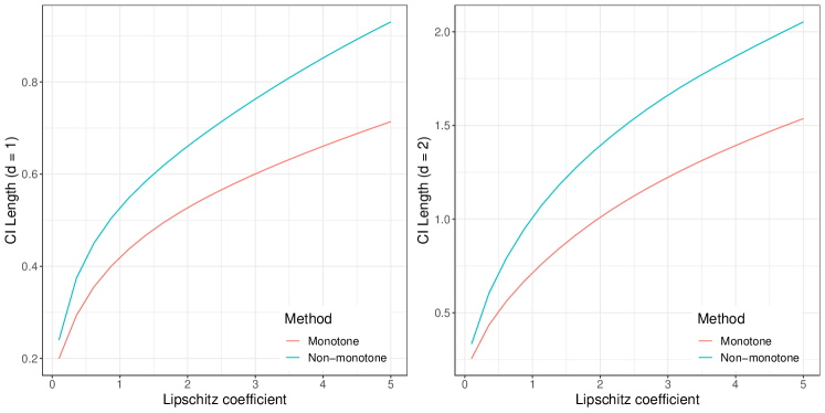
Figure 1: Comparison of the minimax lengths with and without monotonicity. For the design of the running variable(s), 500 observations were generated from the uniform distribution over $[-1,1]^{d}$, for $d=1,2$. When $d=2$, we set $\mathcal{V}=\{1,2\}$ and used the $l_{1}$ norm. The lengths were calculated for $\sigma(x)=1$.

By a similar argument, the length of the minimax CI becomes shorter when we only consider the space of monotone functions. Since the length of the CI is a fixed quantity, we can easily compare its length under the shape restriction to the one without it. Figure 1 considers the cases with $d=1$ and $2$, for the treatment design where individuals are treated when the values of all the running variables are negative. The CI which does not take into account monotonicity can be as much as 30% longer for $d=1$ and 40% longer for $d=2$. Considering the prevalence of RDDs with monotone regression functions, this efficiency gain demonstrates the importance of incorporating the shape restriction when constructing minimax CIs.

4 Adaptive One-sided CI

A prominent feature of the minimax two-sided is that it is a fixed-length CI, in the sense that its length is determined before observing the realization of the outcome $\left\{y_{i}\right\}_{i=1}^{n}$. The length of the CI depends on the Lipschitz constant $C$ chosen by the researcher, and the larger the value of $C$, the longer the CI is. Hence, the minimax CI may become too wide to use in the case where a researcher desires to strengthen the credibility of the inference result by setting a conservative value of the Lipschitz constant. In an extreme case where a researcher wishes to set $C=\infty$, the CI is necessarily the entire real line, providing no information.

To deal with this issue, we provide a method to construct an adaptive one-sided CI. The CI can be made to maintain coverage over a function space with a large Lipschitz constant $C$, even allowing for $C=\infty$. Moreover, as long as the true regression function lies in a smoother class, the length of the CI does not depend on $C$ when $d=1$ and nearly so when $d>1$. In Section 4.1, we discuss this property in more detail, and provide a simple condition on the relationship between the treatment allocation rule and the direction of monotonicity under which such a property holds. This property ensures that a researcher can strengthen the credibility of the inference result by considering a large function space without ending up with an uninformative CI.

Furthermore, the one-sided CI can be made to utilize the information about the smoothness of the unknown regression function $f$ contained in the observed outcome $\{y_{i}\}_{i=1}^{n}$. By using this information, the length of the CI is adjusted accordingly, unlike the minimax optimal CI whose length is fixed regardless of the values of the observed outcome. The CIs possessing this type of property are called adaptive CIs, following Cai and Low (2004). This property further improves the usefulness of the proposed one-sided CI; the length of the CI is not only (nearly) independent of $C$ but shrinks when the true regression function has a smaller first derivative bound.

We focus our discussion on the construction of adaptive lower CIs and related treatment allocation rules. In many RDD applications, researchers are often interested in how significantly larger than 0 the true treatment effect is. In this context, a lower one-sided CI provides useful information. The upper CI can be dealt with in an analogous manner, but requires different (or “opposite”) treatment allocation rules. Lastly, the “length” of a one-sided CI refers to the distance between the true parameter $L_{RD}f$ and its endpoint, referred to as the “excess length” in Armstrong and Kolesár (2018a).

4.1 Conditions on treatment allocation

In this section, we describe in more detail the treatment allocation rules under which it is possible to construct a lower CI with uniform coverage over $\mathcal{F}(C)$, but with length that does not necessarily increase with $C$. Specifically, given a smaller Lipschitz constant $C^{\prime}$ such that $0\leq C^{\prime}<C$, we ask when it is possible to construct a lower CI whose worst-case expected length over $\mathcal{F}(C^{\prime})$ does not grow with $C$. This property ensures that more credibility does not necessarily lead to wider CIs.

To give an intuition, we first describe the argument in a simple setting, where there is a single running variable with the cutoff point $x=0$. Consider a lower CI $[\widehat{L}-\chi^{L},\infty)$ constructed by subtracting a constant $\chi^{L}$ from a linear estimator $\widehat{L}$. In order to maintain uniform coverage over a function space $\mathcal{F}(C)$, we must have

$$\chi^{L}=\sup_{f\in\mathcal{F}(C)}\text{bias}_{f}(\widehat{L})+\text{sd}(\widehat{L})\cdot z_{1-\alpha}.$$

Note that the estimator $\widehat{L}$ we consider is given as the difference between estimators for $f_{t}(0)$ and $f_{c}(0)$, say $\hat{f}_{t}(0)-\hat{f}_{c}(0)$.

Now, suppose individuals receive some treatment if and only if $x_{i}<0$. A key property under this design is that $\hat{f}_{t}(0)$ always has a negative bias if $f_{t}(x)$ is increasing, since $\hat{f}_{t}(0)$ is calculated only using observations with $x_{i}<0$. Similarly, $\hat{f}_{c}(0)$ always has positive bias when $f_{c}(x)$ is increasing. Therefore, the bias of $\widehat{L}$ over $f\in\mathcal{F}(C)$ is always negative, regardless of the value of $C$ specified by the researcher. Hence, a one-sided lower CI that maintains uniform coverage over $\mathcal{F}(C)$ can be formed to be independent of $C$. We can also easily see that this argument no longer holds when the individual $i$ is treated if and only if $x_{i}\geq 0$, in which case the maximum bias over $f\in\mathcal{F}(C)$ increases with $C$.

We now state this idea formally, including the case where $d>1$. Given some $\widetilde{C}>0$, let $\mathcal{L}_{\alpha}(\widetilde{C})$ denote the set of lower CIs (as functions of $\{y_{i}\}_{i=1}^{n}$ and $\{x_{i}\}_{i=1}^{n}$) with uniform coverage probability $1-\alpha$ over $\mathcal{F}(\widetilde{C})$, i.e,

$$CI\in\mathcal{L}_{\alpha}(\widetilde{C})\Longleftrightarrow\inf_{f\in\mathcal{F}(\widetilde{C})}P(L_{RD}f\in CI)\geq 1-\alpha.$$

Now, consider the following quantity:

$$\ell(C^{\prime};C):=\inf_{[\hat{c},\infty)\in\mathcal{L}_{\alpha}(C)}\sup_{f\in\mathcal{F}(C^{\prime})}E[L_{RD}f-\hat{c}],$$ (12)

where $C^{\prime}\leq C$. This is the worst-case expected length of a CI 1) which has correct uniform coverage over $\mathcal{F}(C)$ and 2) whose worst-case expected length is the smallest over $\mathcal{F}(C^{\prime})$. Armstrong and Kolesár (2018a) calculate this quantity in terms of the modulus of continuity defined in Appendix A. The question we ask here is under what conditions the quantity $\ell(C^{\prime};C)$ can be viewed as independent of $C$. In other words, we characterize when it is possible to construct a one-sided lower CI whose length does not grow with $C$ when the regression function belongs to a smoother function space.

Lemma 4.1.

Suppose both $\mathcal{X}_{t}$ and $\mathcal{X}_{c}$ are non-empty, and Assumption 1 holds. Then, given a pair of Lipschitz constants $(C^{\prime},C)$ such that $C^{\prime}<C$, there exists some constant $A(C^{\prime})$, independent of $C$, such that

$$\ell(C^{\prime};C)\leq A(C^{\prime}),$$

if and only if the followings hold: 1) there exists $x_{i}\in\mathcal{X}_{t}$ such that $x_{i}\in(-\infty,0]^{d}$, 2) there exists $x_{i}\in\mathcal{X}_{c}$ such that $x_{i}\in[0,\infty)^{d}$, and 3) the regression function is fully monotone, i.e., $\mathcal{V}=\{1,...,d\}$.

Under the conditions provided in Lemma 4.1, the researcher can construct a one-sided CI whose worst-case expected length is not too large if the true regression function belongs to a smoother space $\mathcal{F}(C^{\prime})$, while maintaining a stringent coverage requirement by specifying a large $C$. When $d=1$, it is possible to take $A(C^{\prime})=\ell(C^{\prime};C^{\prime})$ with the inequality in Lemma 4.1 holding with equality, as suggested by the intuition discussed above. That is, $C$ does not affect the size of $\ell(C^{\prime};C)$ at all when $d=1$. On the other hand, when $d>1$, the same property does not hold unless we have observations only over $[0,\infty)^{d}$ and $(-\infty,0]^{d}$, which is usually not the case in practice. Therefore, specifying a larger $C$ translates into a longer CI (by giving less weights to observations outside $[0,\infty)^{d}\cup(-\infty,0]^{d}$) when $d>1$. However, there is an upper bound on how much this length can grow with $C$. This upper bound is independent of $C$, and thus the worst-case length of the CI is nearly independent of $C$.

In words, the conditions in Lemma 4.1 imply that “the more disadvantaged group should get treated.” Such RDD settings can be easily found in the education literature where students or schools with lower academic performance receive some kind of support (Chay et al., 2005; Chiang, 2009; Jacob and Lefgren, 2004; Leuven et al., 2007; Matsudaira, 2008), in the environmental economics literature where counties with high pollution levels are exposed to some environmental regulations (Chay and Greenstone, 2005; Greenstone and Gallagher, 2008), and in poverty programs which provide funds to those in need (Ludwig and Miller, 2007). Lastly, we note that when the mean potential outcome functions are decreasing rather than increasing, we may simply switch the conditions for $\mathcal{X}_{t}$ and $\mathcal{X}_{c}$ in Lemma 4.1.

4.2 Class of adaptive procedures

Under treatment allocation rules considered in the previous section, it is possible to construct a one-sided CI that is optimal for a single function space $\mathcal{F}(C^{\prime})$ for some $C^{\prime}$, with its length independent or nearly independent of the larger Lipschitz constant $C$. Ideally, we would use a one-sided CI that performs well over a range of function spaces, corresponding to a range of Lipschitz constants $C^{\prime}\in[\underline{C},\overline{C}]$ for some specified bounds $\underline{C}$ and $\overline{C}$. To this end, we define a class of adaptive procedures so that our procedure is based on multiple CIs which solve the optimization problem (12) for different values of Lipschitz constants $C^{\prime}\in\{C_{j}\}_{j=1}^{J}$, with $\underline{C}\leq C_{1}<\cdots<C_{J}\leq\overline{C}$. For now, we assume $(C_{j})_{j=1}^{J}$ are given. We discuss how to choose this sequence of Lipschitz constants in a way that is optimal later on.

To introduce our procedure, we first characterize the solution to (12), applying the general result of Armstrong and Kolesár (2018a) to our setting. Given a value of $C^{\prime}$, it turns out that the lower CI which solves (12) is based on a linear estimator $\widehat{L}(C^{\prime}):=a(C^{\prime})+\sum_{i=1}^{n}w_{i}(C^{\prime})y_{i}$ for non-negative weights $w_{i}(C^{\prime})$ and a centering constant $a(C^{\prime})$. Given some $\tau\in(0,1)$, the endpoint of the lower CI which maintains the uniform coverage probability $1-\tau$ over $\mathcal{F}(C^{\prime})$, takes the form of

$$\hat{c}^{L}_{\tau}(C^{\prime})=\widehat{L}_{\tau}(C^{\prime})-\underset{f\in\mathcal{F}\left(C\right)}{\sup}\text{bias}_{f}(\widehat{L}_{\tau}(C^{\prime}))-z_{1-\tau}\,\text{sd}(\widehat{L}_{\tau}(C^{\prime})).$$ (13)

Here, we make the dependence on $\tau$ explicit because we later choose a suitable $\tau<\alpha$ when $J>1$.

For the estimator, we take $\widehat{L}_{\tau}(C^{\prime})$ to be the difference between two kernel regression estimators, say $\widehat{L}_{t,\tau}(C^{\prime})-\widehat{L}_{c,\tau}(C^{\prime})$, where

$$\widehat{L}_{q,\tau}(C^{\prime}):=\frac{\sum_{x_{i}\in\mathcal{X}_{q}}K(x_{i},h_{q,\tau}(C^{\prime}))y_{i}/\sigma^{2}(x_{i})}{\sum_{x_{i}\in\mathcal{X}_{q}}K(x_{i},h_{q,\tau}(C^{\prime}))/\sigma^{2}(x_{i})},\text{ for each }q\in\{t,c\}.$$

The optimal bandwidths are given by

$$\begin{aligned} h_{t,\tau}(C^{\prime})&=\omega_{t}^{*}\left(z_{1-\tau};C,C^{\prime}\right)\cdot\left({1}/{C},{1}/{C^{\prime}}\right)\text{ and}\\ h_{c,\tau}(C^{\prime})&=\omega_{c}^{*}\left(z_{1-\tau};C^{\prime},C\right)\cdot\left({1}/{C^{\prime}},{1}/{C}\right),\end{aligned}$$ (14)

which completes the definition of the estimator $\widehat{L}_{\tau}(C^{\prime})$. The worst-case bias and the standard deviation of $\widehat{L}_{\tau}(C^{\prime})$ are given by

$$\begin{aligned} \text{sd}(\widehat{L}_{\tau}(C^{\prime}))&=s(z_{1-\tau},h_{t,\tau}(C^{\prime});C,C^{\prime},\sigma^{2}(\cdot))\\ \sup_{f\in\mathcal{F}(C)}\text{bias}(\widehat{L}_{\tau}(C^{\prime}))&=a_{t}(h_{t,\tau}(C^{\prime});C,C^{\prime})-a_{c}(h_{c,\tau}(C^{\prime}),C^{\prime},C)\\[-5.16663pt] &+\frac{1}{2}[\omega_{t}^{*}\left(z_{1-\tau};C,C^{\prime}\right)+\omega_{c}^{*}\left(z_{1-\tau};C^{\prime},C\right)-z_{1-\tau}\,\text{sd}(\widehat{L}_{\tau}(C^{\prime}))],\end{aligned}$$ (15)

which concludes the form of the one-sided CI which solves (12).

The CI $\left[\hat{c}_{\tau}^{L}(C^{\prime}),\infty\right)$ is in terms of the worst-case excess length over $\mathcal{F}(C^{\prime})$ for a single Lipschitz constant $C^{\prime}$. We construct a CI which performs well over a collection of function spaces by taking intersection of CIs in the form of $\left[\hat{c}_{\tau}^{L}(C^{\prime}),\infty\right)$ for different values of $C^{\prime}$. Note that taking the intersection “picks out” the shortest CI among multiple CIs formed. This is roughly equivalent to inferring from the data the true function space where the regression function belongs to, and using the CI which performs well over that function space.

The value of $\tau$ should be calibrated so that the resulting CI maintains correct coverage probability $1-\alpha$ after taking the intersection. Suppose we have a collection of $J$ CIs $\left\{\left[\hat{c}_{\tau}^{L}(C_{j}),\infty\right)\right\}_{j=1}^{J}$. A simple procedure to take the intersection of such CIs is to use a Bonferroni procedure and take $\tau=\alpha/J$. This procedure, however, is conservative since the correlations among the estimators $\widehat{L}_{\tau}(C_{1}),...,\widehat{L}_{\tau}(C_{J})$ are positive, and highly so when $C_{j}$ and $C_{k}$ are close. To calibrate the value of $\tau$ taking into account such positive correlation, let $(V_{j,\tau})_{j=1}^{J}$ denote a $J$-dimensional multivariate normal random variable centered at zero, unit variance, and with covariance terms given as

$$\begin{aligned} \text{Cov}(V_{j,\tau},V_{k,\tau})=&\frac{\sum_{x_{i}\in\mathcal{X}_{t}}K(x_{i},h_{t,\tau}(C_{j}))K(x_{i},h_{t,\tau}(C_{k}))/\sigma^{2}(x_{i})}{z_{1-\tau}^{2}/\omega_{t}^{*}\left(z_{1-\tau};C,C_{j}\right)\omega_{t}^{*}\left(z_{1-\tau};C,C_{k}\right)}\\ &+\frac{\sum_{x_{i}\in\mathcal{X}_{c}}K(x_{i},h_{c,\tau}(C_{j}))K(x_{i},h_{c,\tau}(C_{k}))/\sigma^{2}(x_{i})}{z_{1-\tau}^{2}/\omega_{c}^{*}\left(z_{1-\tau};C_{j},C\right)\omega_{c}^{*}\left(z_{1-\tau};C_{k},C\right)}.\end{aligned}$$ (16)

Then, we can show that if we take $\tau^{*}$ to be the value of $\tau$ that solves

$$P\left(\max_{1\leq j\leq J}V_{j,\tau}>z_{1-\tau},\right)=\alpha,$$ (17)

then the resulting CI obtained by taking the intersection has correct coverage. Regarding the solution to the above equation, we can actually show that $\text{Cov}(V_{j,\tau},V_{k,\tau})$ does not depend on $\tau$ as $n\to\infty$, which implies that $\max_{1\leq j\leq J}V_{j,\tau^{*}}$ converges in distribution to a random variable $V_{\max}$ which does not dependent on $\tau$. The following is the main theoretical result for our intersection CI.

Theorem 4.2.

Given $\{C_{1},...,C_{J}\}$, $C$ and $\alpha\in(0,1)$, let $\tau^{*}$ be defined as in (17). Then, under Assumption 1, if we let $\hat{c}:=\max_{1\leq j\leq J}\hat{c}_{\tau^{*}}^{L}(C_{j})$, we have

$$\inf_{f\in\mathcal{F}(C)}P_{f}\left(L_{RD}f\in[\hat{c},\infty)\right)\geq 1-\alpha.$$

The next result, which is immediate from Armstrong and Kolesár (2018a), shows that the class of adaptive procedures we consider is a reasonable one. It basically states that each of the CIs $[\hat{c}_{\tau^{*}}^{L}(C_{j}),\infty)$ is an optimal CI when $f\in\mathcal{F}(C_{j})$, except that it covers the true parameter with probability $1-\tau^{*}$ instead of $1-\alpha$, which is the price we pay to adapt to multiple Lipschitz classes.

Corollary 4.3.

Under Assumption 1, $[\hat{c}_{\tau^{*}}^{L}(C_{j}),\infty)$ solves

$$\inf_{[\hat{c},\infty)\in\mathcal{L}_{\tau^{*}}(C)}\sup_{f\in\mathcal{F}(C_{j})}E_{f}[L_{RD}f-\hat{c}].$$

Again, considering the simple case where $d=1$ and $\mathcal{V}=\{1\}$ provides an intuition behind our adaptive procedure. Under this simple case, $\widehat{L}_{q,\tau}(C^{\prime})$ is simply a kernel regression estimator with kernel $K(z)=[1-|z|]_{+}$ and bandwidths

$$h_{t,\tau}(C^{\prime})=\omega_{t}^{*}\left(z_{1-\tau};C,C^{\prime}\right)/C^{\prime},\quad h_{c,\tau}(C^{\prime})=\omega_{c}^{*}\left(z_{1-\tau};C^{\prime},C\right)/C^{\prime}.$$ (18)

Applying results of Kwon and Kwon (2020), we can show that these quantities are approximately $c\times(C^{\prime})^{-2/3}$ for some constant $c$ for large $n$. This implies that we construct estimators with varying bandwidth sizes, and compare the lengths of resulting one-sided CIs. The estimator with a smaller bandwidth is the one constructed to perform well when the Lipschitz constant of the regression function is large, and vice versa for the estimator with a larger bandwidth. This is because when the Lipschitz constant of the regression function is large, the excess length of a one-sided CI is reduced by taking a smaller bandwidth to decrease the absolute size of the bias. On the other hand, when the Lipschitz constant of the regression function is small, reducing the standard deviation by taking a larger bandwidth matters more in reducing the excess length of a one-sided CI. This idea is similar to the bandwidth snooping procedure suggested by Armstrong and Kolesár (2018b). The results therein focus on the case with a single running variable and adapting to the Hölder exponent.

Remark 4 (Specifying $C$).

When $d=1$, the worst-case bias is 0 under the treatment allocation rules in Section 4.1. Therefore, a researcher can set $C=\infty$ and not worry about correct coverage. On the other hand, when $d>1$, the size of $C$ governs how large weights should be on observations outside $[0,\infty)^{d}$ and $(-\infty,0]^{d}$. A larger $C$ puts smaller weights on those observations, leading to a wider CI, with $C=\infty$ corresponding to using observations only in $[0,\infty)^{d}$ and $(-\infty,0]^{d}$. However, the length of the adaptive CI shrinks when the true regression function has a smaller first derivative bound even if $C$ is set to be a large number, alleviating the concern that large $C$ might lead to a less informative CI.

Remark 5 (Adaptation in multi-dimensional RDDs).

Consider the setting of Remark 2, where the Lipschitz continuity is specified by the weighted $\ell_{1}$-norm with Lipschitz constants $C_{1},...,C_{d}$. Then, our adaptive procedure allows one to consider different values of $C$ other than $C=1$. Note that this takes $C_{1}/C_{s}$ given for $s=2,...,d$. Adapting to different values of $C_{1}/C_{s}$ is an interesting extension that we did not pursue here.

4.3 Choice of an adaptive procedure

In this section, we discuss the choice of Lipschitz constants $(C_{j})_{j=1}^{J}$ to conclude our definition of the adaptive one-sided CI. The choice of function spaces to adapt to is especially relevant in our setting unlike the previous literature on adaptive inference. The previous literature has mostly focused on rate-adaptation, the problem of how to construct a CI which shrinks at an optimal rate. For example, Armstrong (2015) and Armstrong and Kolesár (2018b) discuss adaptive testing and construction of adaptive CIs for the RD parameter, which adapt to Hölder exponents $\beta\in(0,1]$. In this case, since different Hölder exponents imply different convergence rates, adapting to the entire continuum of Hölder exponents is in some sense always optimal. On the other hand, when we fix $\beta=1$ and try to adapt to Lipschitz constants, the convergence rate is always $n^{1/(2+d)}$, and what matters is the actual length of CIs, not their rate of convergence.

The optimal but infeasible adaptive CI is given as $CI=[\hat{c},\infty)$ such that

$$\sup_{f\in\mathcal{F}(C^{\prime})}E[L_{RD}f-\hat{c}]=\ell(C^{\prime};C),$$

for all $C^{\prime}\in[\underline{C},\overline{C}]$, where $\ell(C^{\prime};C)$ is defined in (12). This is infeasible since the form of CI which is optimal over $\mathcal{F}(C^{\prime})$ is different from the one which is optimal over $\mathcal{F}(C^{\prime\prime})$ for $C^{\prime}\neq C^{\prime\prime}$. Instead, our aim is to construct a CI $[\hat{c},\infty)$ such that

$$\ell^{\text{adpt}}(C^{\prime}):=\sup_{f\in\mathcal{F}(C^{\prime})}E[L_{RD}f-\hat{c}]$$

is close to $\ell(C^{\prime};C)$ over $C^{\prime}\in\left[\underline{C},\overline{C}\right]$ given some $\left(\underline{C},\overline{C}\right)$, when $\ell^{\text{adpt}}(C^{\prime})$ and $\ell(C^{\prime};C)$ are viewed as a function of $C^{\prime}$.

Procedure 2 Adaptive One-sided CI.

1. Choose $C$ so that the Lipschitz continuity in (2) is satisfied, with a suitable choice of a norm $||\cdot||$ on $\mathbb{R}^{d}$ when $d>1$. - When $d=1$, we can set $C=\infty$; see Remark 4 in Section 4.2. 2. Choose values of $\underline{C}$ and $\overline{C}$ such that $0\leq\underline{C}<\overline{C}\leq C$, which is the region where the adaptive CI will be close to optimal. - A reasonable value of $\underline{C}$ can be estimated; see Appendix B. 3. Let $\mathcal{C}(J)$ be the equidistant grid of size $J$ over $\left[\underline{C},\overline{C}\right]$. Starting from $J=2$, increase $J$ by $1$ until $\lvert\Delta(\mathcal{C}(J))-\Delta(\mathcal{C}(J-1))\rvert\leq\varepsilon$, for a tolerance level $\varepsilon$. 4. Let $J^{*}$ be the value of $J$ we stopped at in Step 3. We use $\mathcal{C}(J^{*})=(C_{j})_{j=1}^{J^{\ast}}$ as the sequence of Lipschitz constants to construct the adaptive CI. 5. Using (13), (14), (15), and (17), finally obtain the adaptive one-sided CI, $$\Big{[}\max_{1\leq j\leq J}\hat{c}_{\tau^{*}}^{L}(C_{j}),\infty\Big{)}.$$

By restricting the class of one-sided CIs to those considered in Section 4.2, we can show that there is a measure of distance between $\ell^{\text{adpt}}(\cdot)$ and $\ell(\cdot;C)$ which is both reasonable and easy to calculate. To be specific, let $\mathcal{C}=(C_{j})_{j=1}^{J}$ denote some sequence of Lipschitz constants to be used to construct our adaptive CI, and denote the endpoint of the CI with $\hat{c}(\mathcal{C})$. Then, write

$$\ell^{\text{adpt}}(C^{\prime};\mathcal{C}):=\sup_{f\in\mathcal{F}(C^{\prime})}E[L_{RD}f-\hat{c}(\mathcal{C})].$$

Consider the following quantity measuring the “distance” between $\ell^{\text{adpt}}(\cdot;\mathcal{C})$ and $\ell(\cdot;C)$:

$$\Delta(\mathcal{C}):=\sup_{C^{\prime}\in\left[\underline{C},\overline{C}\right]}\frac{\ell^{\text{adpt}}(C^{\prime};\mathcal{C})}{\ell(C^{\prime};C)}.$$ (19)

Note that this criterion is consistent with the previous literature which compares the performances of different confidence intervals using a ratio measure (Cai and Low, 2004; Armstrong and Kolesár, 2018a). Specifically, $\Delta(\mathcal{C})$ satisfies

$$\ell^{\text{adpt}}(C^{\prime};\mathcal{C})\leq\Delta(\mathcal{C})\ell(C^{\prime};C),\ \forall C^{\prime}\in\left[\underline{C},\overline{C}\right].$$

This is the precisely the notion of adaptive CIs introduced in Cai and Low (2004). Since the rates of $\ell^{\text{adpt}}(C^{\prime};\mathcal{C})$ and $\ell(C^{\prime};C)$ are the same under our setting, the choice of an adaptive procedure should be based on the size of the constant $\Delta(\mathcal{C})$.

An advantage from focusing on the class of adaptive CIs proposed in Section 4.2 is that it is easy to evaluate $\Delta(\mathcal{C})$ as shown in the following proposition.

Proposition 4.4.

We have $\ell^{\text{adpt}}(C^{\prime};\mathcal{C})=E\min_{j\leq J}U_{j}$, where $U:=(U_{1},\dots,U_{J})^{\prime}$ is a Gaussian random vector with known mean and variance. Furthermore, we have

$$\ell(C^{\prime};C)=\omega_{t}^{*}(z_{1-\alpha},C,C^{\prime})+\omega_{c}^{*}(z_{1-\alpha},C^{\prime},C).$$

Based on the discussion so far, we recommend choosing $\{C_{j}\}_{j=1}^{J}$ based on the value of $\Delta(\mathcal{C})$. When calculating this value, searching for all possible sequences $\mathcal{C}$ is infeasible in practice. Instead, we suggest taking $\mathcal{C}=\mathcal{C}(J)$ to be the equidistant grid of size $J$ on $\left[\underline{C},\overline{C}\right]$ and calculating $\Delta(\mathcal{C}(J))$ for different values of $J$. Our simulation study (not reported) suggests that the gain from increasing $J$ becomes very small after some threshold. Hence, a computationally attractive procedure is to increase the value of $J$ until the additional gain from using $J+1$ instead of $J$ is smaller than a tolerance parameter. In the simulation designs of Section 5, the largest value of $\Delta(\mathcal{C}(J^{*}))$ across all scenarios is less than 1.07, where $J^{*}$ is the value of $J$ obtained by the method described above. That is, the worst-case length of the adaptive CI is at most $7$% longer than the worst-case length of the CI that we would have used if we knew the true Lipschitz constant, in the data generating processes considered in Section 5.

Note that our procedure requires a researcher to specify the values of $\underline{C}$ and $\overline{C}$. For $\underline{C}$, while it can be set to 0, a reasonable value of $\underline{C}$ can be estimated from the data as discussed in Appendix B. The value of $\overline{C}$ defines a region for Lipschitz constants where the adaptive CI is intended to perform well. Therefore, a researcher may choose $\overline{C}$ to be some non-conservative potential value of the Lipschitz constant of the regression function. As discussed above, the coverage probability is not affected whatever the value of $\overline{C}$ is, so it will not be a burdensome task for a researcher to choose $\overline{C}$. Procedure 2 summarizes the steps for constructing the adaptive one-sided CI, including the choice of the Lipschitz spaces to adapt to.

5 Monte Carlo Simulations

	$x_{i}\sim\text{unif}(-1,1)$	Constant variance	$C$ is small
Design 1	YES	YES	YES
Design 2	NO	YES	YES
Design 3	YES	NO	YES
Design 4	NO	NO	YES
Design 5	YES	YES	NO
Design 6	NO	YES	NO
Design 7	YES	NO	NO
Design 8	NO	NO	NO

Table 1: Simulation design specifications

We investigate the performance of our minimax and adaptive procedures via a simulation study. We focus on the case where $d=1$ with individuals being treated if $x_{i}<0$. We restrict the support of $x_{i}$ to be $[-1,1]$. For a given true sharp RDD parameter $\theta\equiv L_{RD}f$, we consider the following designs.

1. Linear design: $f_{1c}(x)=Cx$, $f_{1t}(x)=f_{1c}(x)+\theta$. We have $|f_{1q}^{\prime}(x)|=C$, and $|f_{1q}^{\prime\prime}(x)|=0$ for all $x\in[-1,1]$ and $q\in\{t,c\}$.

2. Modified specification of Armstrong and Kolesár (2018c): given some “knots” $(b_{1},b_{2})$ such that $0<b_{1}<b_{2}$, define

   $$f_{2c}(x)=\frac{3C}{2}(x^{2}-2(x-b_{1})_{+}^{2}+2(x-b_{2})_{+}^{2}),\hskip 15.0ptf_{2t}(x)=-f_{2c}(-x)+\theta.$$

   If $b_{1}\geq b_{2}/2$, both functions are increasing. Taking $(b_{1},b_{2})=(1/3,2/3)$ gives $|f_{2q}^{\prime}(x)|\leq C$, and $|f_{2q}^{\prime\prime}(x)|=3C$ for all $x\in[-1,1]$ and $q\in\{t,c\}$. We also have $|f_{2q}^{\prime}(0)|=0$.

3. Modified specification of Babii and Kumar (2020): define

   $$f_{3c}(x)=\frac{C}{4}(x^{3}+x),\hskip 15.0ptf_{3t}(x)=f_{3c}(x)+\theta.$$

   We have $|f_{3q}^{\prime}(x)|\leq C$ and $|f_{3q}^{\prime\prime}(x)|=3C/2$ for all $x\in[-1,1]$ and $q\in\{t,c\}$. We also have $|f_{3q}^{\prime}(0)|=C/4$ and $|f_{3q}^{\prime\prime}(0)|=0$.

4. Nonzero first and second derivatives at $0$: define

   $$f_{4c}(x)=C((3x+1)^{1/3}-1),\hskip 15.0ptf_{4t}(x)=-f_{4c}(-x)+\theta.$$

   We have $|f_{4q}^{\prime}(x)|\leq C$, and $|f_{4q}^{\prime\prime}(x)|\leq 2C$ for all $x\in[-1,1]$ and $q\in\{t,c\}$. We also have $|f_{4q}^{\prime}(0)|=C$ and $|f_{4q}^{\prime\prime}(0)|=2C$.

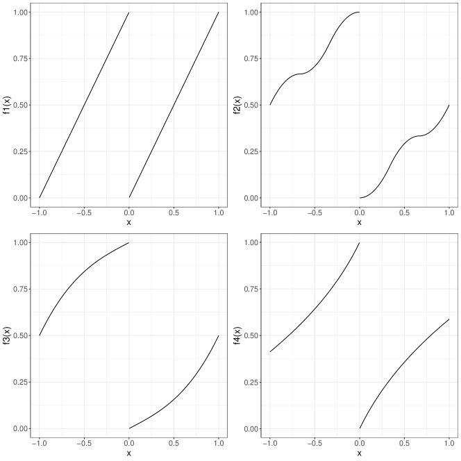
Figure 4: Regression function values on $x\in[-1,1]$.

For the running variables, we consider $x_{i}\sim\text{unif}(-1,1)$ and $x_{i}\sim 2\times\text{Beta}(2,2)-1$. The latter is used by Babii and Kumar (2020), and gives more observations around the cutoff. Finally, we consider both homoskedastic and heteroskedastic designs, $\sigma_{1}(x)=1$ and $\sigma_{2}(x)=\phi(x)/\phi(0)$, where $\phi(x)$ is the standard normal pdf. The sample size is $n=500$. Figure 4 in Appendix D provides plots for the four regression functions.

We estimate the conditional variance based on local constant kernel regression, where the initial bandwidth is chosen based on Silverman’s rule of thumb. This is to avoid using a bandwidth selection method based on local linear regression to ensure that our proposed method works even when the second derivative is very large. After the estimators are calculated based on the estimated conditional variance, we construct the CIs following Armstrong and Kolesár (2020b), who use a simple way to estimate the variance by

$$\hat{\sigma}(x_{i})^{2}=\frac{J}{J+1}\left(y_{i}-\frac{1}{J}\sum_{i=1}^{J}y_{j(i)}\right)^{2},$$

for some fixed $J$, where $j(i)$ denotes the index for the closest observation to $i$ (with the same treatment status). The default value in their implementation is $J=3$, which we follow.

	$f=f_{1}$			$f=f_{2}$
	Length:	RBC	Minimax	Length:	RBC	Minimax
	RBC/MM	coverage	coverage	RBC/MM	coverage	coverage
Design 1	1.094	0.925	0.968	1.097	0.924	0.942
Design 2	1.112	0.938	0.979	1.115	0.941	0.949
Design 3	1.082	0.926	0.968	1.085	0.924	0.942
Design 4	1.099	0.936	0.979	1.103	0.940	0.950
Design 5	1.128	0.925	0.919	1.148	0.930	0.945
Design 6	1.137	0.938	0.934	1.162	0.941	0.951
Design 7	1.117	0.926	0.920	1.139	0.927	0.945
Design 8	1.125	0.936	0.935	1.153	0.941	0.952

Table 2: Comparison between RBC and minimax; $f\in\{f_{1},f_{2}\}$

5.1 Minimax procedure

First, we investigate the performance of the minimax procedure described in Section 3. We consider different combinations of specifications on the running variable, the variance function, and the value of $C$: 1) $x_{i}$ follows either a uniform or a Beta distribution, 2) the variance function is given by either $\sigma^{2}\times\sigma_{2}^{1}(x)$ or $\sigma^{2}\times\sigma_{2}^{2}(x)$ (where $\sigma^{2}=1/4$), and 3) the true value of $C$ is either small ($C=1$) or large ($C=3$). For the minimax two-sided CI, we consider the case where we correctly specify the Lipschitz constant in all cases, setting $C=3$. The results were calculated with $1,000$ repetitions. The definition of each design is given in Table 1.

	$f=f_{3}$			$f=f_{4}$
	Length:	RBC	Minimax	Length:	RBC	Minimax
	RBC/MM	coverage	coverage	RBC/MM	coverage	coverage
Design 1	1.090	0.925	0.949	1.093	0.924	0.968
Design 2	1.109	0.937	0.951	1.111	0.938	0.977
Design 3	1.078	0.925	0.949	1.081	0.924	0.968
Design 4	1.096	0.936	0.953	1.098	0.936	0.977
Design 5	1.094	0.923	0.962	1.119	0.920	0.930
Design 6	1.112	0.937	0.971	1.132	0.935	0.947
Design 7	1.082	0.924	0.961	1.107	0.924	0.930
Design 8	1.099	0.936	0.971	1.119	0.933	0.947

Table 3: Comparison between RBC and minimax; $f\in\{f_{3},f_{4}\}$

We measure the performance of the minimax procedure by comparing it to one of the robust bias correction (RBC) procedures by Calonico et al. (2015). We report ratios of the average length of the CI between the RBC and the minimax procedure, as well as their respective coverage probabilities. For the robust bias correction procedure, we use the default implementation provided the R package rdrobust.

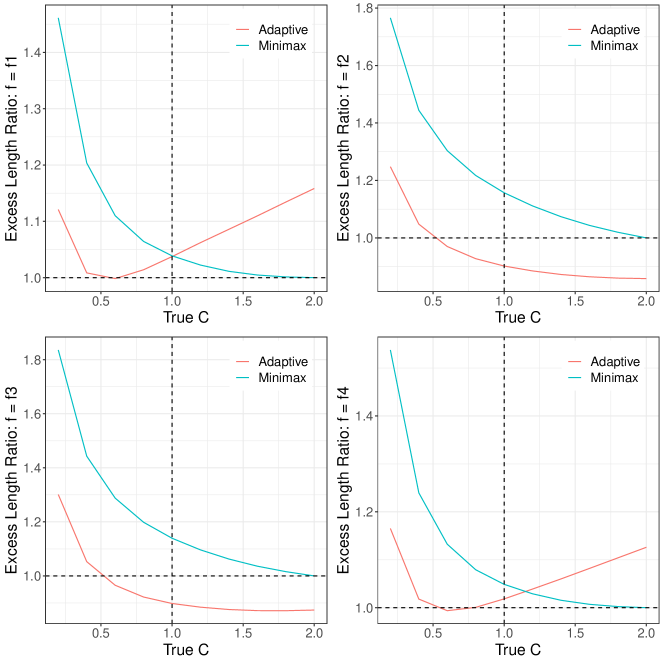
Figure 2: Performance comparison of one-sided CIs

Tables 2 and 3 display the results. For each regression function, the first column shows the ratio of the length of the CIs, and the second and the third columns show the coverage probabilities of the RBC and the minimax procedures. Despite the fact that the minimax CIs are shorter than the RBC CIs, the coverage probabilities of the minimax CIs are closer to the nominal level than the RBC CIs. However, the length comparison here should not be interpreted as the superiority of our procedure over the RBC method, since the lengths are sensitive to the choice of $C$ and to the form of the true regression function. Rather, as we have discussed so far, the relative advantage of our procedure is the use of a more transparent function space, and incorporating the monotonicity of the regression function.

5.2 Adaptive procedure

Next, we compare the performance of the one-sided CI to two benchmarks, the minimax and the oracle one-sided CIs. Specifically, we consider regression functions $f_{1},...,f_{4}$ and vary the value of $C\in[C_{l},C_{u}]$ which determines their smoothness. For each $C\in[C_{l},C_{u}]$, the oracle procedure adapts to a single Lipschitz constant $C$, as if we know the true Lipschitz constant, which is infeasible in practice. On the other hand, the minimax procedure adapts to the largest Lipschitz constant $C_{u}$; this procedure is nearly optimal (among feasible procedures) when we do not have monotonicity, as shown in Armstrong and Kolesár (2018a). Both the oracle and the minimax procedures take monotonicity into account.

We take $(C_{l},C_{u})=(1/5,2)$ and consider only Design 1. For the adaptive procedure, we take $(\underline{C},\overline{C})=(1/5,1)$. We expect that the performance of the adaptive procedure will be better over $C\in[1/5,1]$ than over $C\in[1,2]$.

Figure 2 shows the relative excess lengths of the minimax and adaptive CIs compared to the oracle procedure. First, we note that the adaptive CIs are at most 30% longer than the oracle procedure, while the minimax CIs are sometimes as much as 83% longer than the oracle. Second, for the case of $f=f_{2}$ and $f=f_{3}$, the adaptive CIs are sometimes even shorter than the oracle. This is because the derivatives of such regression functions near $x=0$ are smaller than $C$, although their maximum derivatives are $C$ globally. This shows that the adaptive CI adapts to the local smoothness of the regression function, which is another advantage of using the adaptive procedure.

6 Empirical Illustration

In this section, we revisit the analysis by Lee (2008). The running variable $x_{i}\in[-100,100]$ is the Democratic margin of victory in each election, and the outcome variable $y_{i}\in[0,100]$ is the Democratic vote share in the next election. The treatment is the incumbency of the Democratic party, with the cutoff given by 0. Therefore, a positive treatment effect indicates that there is an electoral advantage to incumbent candidates.

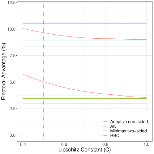
Figure 3: Lee (2008) example. The red line (Minimax two-sided) plots our minimax optimal CI, while the blue line (RBC) and the green line (AK) plot the CIs constructed using the methods of Calonico et al. (2015) and Armstrong and Kolesár (2018a), respectively. The purple line (Adaptive one-sided) plots the adaptive one-sided upper CI with $C=\infty$. The vertical dotted line indicates $C=1/2$, our preferred specification.

This empirical application nicely fits the setting we consider in this paper. For monotonicity, it is plausible to assume that a party’s vote share increases on average in that party’s previous vote share. Moreover, for Lipschitz continuity, it is plausible that a unit increase in the previous election vote share can predict the vote share increase in the next election by no more than a single unit. This reflects the viewpoint that the previous election vote share is a noisy measure of a party’s popularity in the current election. Since $x_{i}$ is the vote margin instead of the vote share, this translates to setting $C=1/2$.

Figure 3 plots the CIs constructed from our minimax optimal procedure for different values of $C\in[0.4,1]$, which includes our preferred specification $C=1/2$. We also include CIs using the robust bias correction method of Calonico et al. (2015) and the minimax CI using a second derivative bound as in Armstrong and Kolesár (2018a). For the latter, the bound on second derivative is set as $M=1/10$, which is the largest bound used in their empirical analysis. The nominal coverage probability is $0.95$ for all CIs. The CIs obtained by the robust bias correction and the second derivative bound are given by $[3.44,8.38]$ and $[2.95,8.96]$, respectively. Our CI has a larger lower bound and upper bound compared to other methods. Especially, at our preferred specification $C=1/2$, the CI is given by $[5.03,9.66]$, implying a potentially larger size of incumbents’ electoral advantage compared to other inference methods. At this specification, our CI is also relatively shorter than others. For the same dataset, Babii and Kumar (2020) give a CI of $[6.6,26.5]$, whose upper bound is larger than other procedures.

As discussed above, since the Lipschitz constant C has a clear interpretation, a sensitivity analysis varying the values of the Lipschitz constant is especially useful in strengthening the credibility of the inference results. Specifically, we can calculate the size of the smoothness parameter under which the effect of incumbency becomes insignificant. It turns out that our minimax CI contains $0$ when $C$ is larger than 16. The first derivative bound $C=16$ roughly implies that one unit increase in the previous election vote share can predict as much as a 32 unit increase in the next election vote share, which is quite a large amount. Therefore, we conclude that the significance of the incumbency effect is robust over a reasonable set of assumptions on the unknown regression function.

Given that various CIs considered here are obtained from different assumptions on the regression function, it would be an interesting exercise to see what we can infer about the RD parameter under a minimal assumption. To this end, we construct an adaptive one-sided CI which maintains coverage over all monotone functions. The discussion in Section 4.1 implies that we can construct an adaptive upper CI in this empirical setting. We take $(\underline{C},\overline{C})=(0.1,0.5)$, reflecting the belief that the true Lipschitz constant is likely to be less than $0.5$. To make the one-sided CI comparable with the other two-sided CIs, the nominal coverage probability of the upper CI is set as $0.975$, and the resulting upper bound is 10.52%. While this upper CI maintains coverage over all monotone functions, the resulting upper bound is not significantly greater than the upper bounds of the other CIs, which reflects the adaptive nature of the upper CI.

7 Conclusion

In this paper, we proposed a minimax two-sided CI and an adaptive one-sided CI when the regression function is assumed to be monotone and has bounded first derivative. We showed our procedure achieves uniform coverage under easy-to-interpret conditions and can be used to construct either a two-sided CI with a minimax optimal length or a one-sided one whose excess length adapts to the smoothness of the unknown regression function. There are two extensions that we find interesting.

Fuzzy RDDs. There are various RDD applications where compliance to a treatment status is only partial. Therefore, it would be of interest to extend our approach to the fuzzy RDD setting, for example, by making monotonicity and Lipschitz continuity assumptions on the treatment propensity $p(x)=P(t_{i}=1|x_{i}=x)$, where $t_{i}$ is the treatment indicator for individual $i$. This approach will complement the minimax optimal approaches to fuzzy RDDs using second derivative bounds by Armstrong and Kolesár (2020b) and Noack and Rothe (2020).

Weigthed CATE. In multi-score RDDs, Imbens and Wager (2019) suggest estimating the weighted average of conditional treatment effects over different boundary points to make inference more precise. Since the weighted average parameter is a linear functional of the regression function, we can also adjust our framework to conduct inference on the parameter. On the other hand, a closed-form solution might not exist, and how to computationally construct the confidence interval for the weighted average parameter under our setting seems to be an interesting research question.

Appendix A Lemmas and Proofs

In this section, we collect auxiliary lemmas and omitted proofs. Before presenting the results, we state the following definition.

Definition 1.

Given two Lipschitz constants $C_{1}$ and $C_{2}$, and some positive constant $\delta\geq 0$, we define

$$\omega\left(\delta;C_{1},C_{2}\right) := \underset{f_{1}\in\mathcal{F}(C_{1}),\ f_{2}\in\mathcal{F}(C_{2})}{\sup}L_{RD}f_{2}-L_{RD}f_{1}$$ (20)

$$\text{s.t.}\sum_{i=1}^{n}\left(\frac{f_{2}(x_{i})-f_{1}(x_{i})}{\sigma(x_{i})}\right)^{2}\leq\delta^{2}.$$

The quantity $\omega\left(\delta;C_{1},C_{2}\right)$ is called the ordered modulus of continuity of $\mathcal{F}(C_{1})$ and $\mathcal{F}(C_{2})$ for the parameter $L_{RD}f$.

A.1 Lemmas

Lemma A.1.

Given some pair of numbers $C,C^{\prime}\geq 0$ and $\delta\geq 0$, define $\omega_{q}(\delta;C,C^{\prime})$ for each $q\in\{t,c\}$ to be the solution to the following equation

$$\sum_{x_{i}\in\mathcal{X}_{q}}\left[\omega_{q}(\delta;C,C^{\prime})-C\left\lVert(x_{i})_{\mathcal{V}+}\right\rVert-C^{\prime}\left\lVert(x_{i})_{\mathcal{V}-}\right\rVert\right]_{+}^{2}/\sigma^{2}(x_{i})=\delta^{2}.$$

Then, we have

$$\omega_{q}(\delta;C,C^{\prime})=\underset{f_{1}\in\mathcal{F}(C),f_{2}\in\mathcal{F}(C^{\prime})}{\sup}f_{2}(0)-f_{1}(0)$$

$$\text{s.t. }\sum_{x_{i}\in\mathcal{X}_{q}}\left(\frac{f_{2}(x_{i})-f_{1}(x_{i})}{\sigma(x_{i})}\right)^{2}\leq\delta^{2}.$$ (21)

Proof.

See Kwon and Kwon (2020). ∎

Lemma A.2.

Given some pair $C_{1},C_{2}\geq 0$ and $\delta\geq 0$, we have

$$\omega\left(\delta;C_{1},C_{2}\right)=\omega_{t}\left(\delta_{t}^{*}\left(\delta;C_{1},C_{2}\right);C_{1},C_{2}\right)+\omega_{c}\left(\delta_{c}^{*}\left(\delta;C_{2},C_{1}\right);C_{2},C_{1}\right).$$

Proof of Lemma A.2.

Noting that

$$L_{RD}f_{2}-L_{RD}f_{1} = \left(f_{2,t}(0)-f_{2,c}(0)\right)-\left(f_{1,t}(0)-f_{1,c}(0)\right)$$

$$= \left(f_{2,t}(0)-f_{1,t}(0)\right)+\left(f_{1,c}(0)-f_{2,c}(0)\right),$$

$\omega\left(\delta;C_{1},C_{2}\right)$ is obtained by solving the following problem:

$$\sup_{f_{1,t},f_{1,c},f_{2,t},f_{2,c}}\left(f_{2,t}(0)-f_{1,t}(0)\right)+\left(f_{1,c}(0)-f_{2,c}(0)\right)$$

s.t. $$\sum_{i=1}^{n}\left(\mathbbm{1}\left\{x_{i}\in\mathcal{X}_{t}\right\}\left(\frac{f_{2,t}(x_{i})-f_{1,t}(x_{i})}{\sigma(x_{i})}\right)^{2}+\mathbbm{1}\left\{x_{i}\in\mathcal{X}_{c}\right\}\left(\frac{f_{1,c}(x_{i})-f_{2,c}(x_{i})}{\sigma(x_{i})}\right)^{2}\right)\leq\delta^{2},$$

$$f_{1,t},f_{1,c}\in\Lambda_{+,\mathcal{V}}\left(C_{1}\right),f_{2,t},f_{2,c}\in\Lambda_{+,\mathcal{V}}\left(C_{2}\right).$$

Using the definitions for $\omega_{t}\left(\delta_{t};C_{1},C_{2}\right)$ and $\omega_{c}\left(\delta_{c};C_{1},C_{2}\right)$, and Lemma A.1, we can write

$$\omega\left(\delta;C_{1},C_{2}\right)=\sup_{\delta_{t}\geq 0,\delta_{c}\geq 0,\delta_{t}^{2}+\delta_{c}^{2}=\delta^{2}}\omega_{t}\left(\delta_{t};C_{1},C_{2}\right)+\omega_{c}\left(\delta_{c};C_{2},C_{1}\right),$$

which concludes the proof. ∎

Lemma A.3.

Given some $\left(C_{1},C_{2}\right)\in\mathbb{R}_{+}^{2}$ and $\delta\geq 0$, write $\delta_{t}^{*}:=\delta_{t}^{*}(\delta;C_{1},C_{2})$, $\delta_{c}^{*}:=\delta_{c}^{*}(\delta;C_{2},C_{1})$. Then, we can find $\left(f_{\delta,1}^{*},f_{\delta,2}^{*}\right)\in\mathcal{F}\left(C_{1}\right)\times\mathcal{F}\left(C_{2}\right)$, which satisfy the following three conditions: (i) $L_{RD}f_{\delta,2}^{*}-L_{RD}f_{\delta,1}^{*}=\omega\left(\delta;C_{1},C_{2}\right)$, (ii) $\left\lVert\frac{f_{\delta,2}^{*}-f_{\delta,1}^{*}}{\sigma}\right\rVert_{2}^{2}=\delta^{2}$, and (iii) when we write

$$f_{\delta,2}^{*} = f_{\delta,2,t}^{*}\mathbbm{1}\left\{x\in\mathcal{X}_{t}\right\}+f_{\delta,2,c}^{*}\mathbbm{1}\left\{x\in\mathcal{X}_{c}\right\}$$

$$f_{\delta,1}^{*} = f_{\delta,1,t}^{*}\mathbbm{1}\left\{x\in\mathcal{X}_{t}\right\}+f_{\delta,1,c}^{*}\mathbbm{1}\left\{x\in\mathcal{X}_{c}\right\},$$

$\left(f_{\delta,1,t}^{*},f_{\delta,2,t}^{*}\right)\in\mathcal{F}\left(C_{1}\right)\times\mathcal{F}\left(C_{2}\right)$ and $\left(f_{\delta,1,c}^{*},f_{\delta,2,c}^{*}\right)\in\mathcal{F}\left(C_{1}\right)\times\mathcal{F}\left(C_{2}\right)$ satisfy

$$f_{\delta,2,t}^{*}-f_{\delta,1,t}^{*} = \left[\omega_{t}\left(\delta_{t}^{*};C_{1},C_{2}\right)-C_{1}\left\lVert(x)_{\mathcal{V}+}\right\rVert-C_{2}\left\lVert(x)_{\mathcal{V}-}\right\rVert\right]_{+}$$ (22)

$$f_{\delta,1,c}^{*}-f_{\delta,2,c}^{*} = \left[\omega_{c}\left(\delta_{c}^{*};C_{2},C_{1}\right)-C_{1}\left\lVert(x)_{\mathcal{V}-}\right\rVert-C_{2}\left\lVert(x)_{\mathcal{V}+}\right\rVert\right]_{+},$$ (23)

$$f_{\delta,1,t}^{*}(0)+f_{\delta,2,t}^{*}(0) = \omega_{t}\left(\delta_{t}^{*};C_{1},C_{2}\right)$$ (24)

$$f_{\delta,1,c}^{*}(0)+f_{\delta,2,c}^{*}(0) = \omega_{c}\left(\delta_{c}^{*};C_{2},C_{1}\right),$$ (25)

and

$$\left(f_{\delta,2,t}^{*}-f_{\delta,1,t}^{*}\right)\left(f_{\delta,1,t}^{*}+f_{\delta,2,t}^{*}\right)$$

$$= \left(f_{\delta,2,t}^{*}-f_{\delta,1,t}^{*}\right)\left(\omega_{t}\left(\delta_{t}^{*};C_{1},C_{2}\right)+C_{1}\left\lVert(x)_{\mathcal{V}+}\right\rVert-C_{2}\left\lVert(x)_{\mathcal{V}-}\right\rVert\right)$$ (26)

$$\left(f_{\delta,1,c}^{*}-f_{\delta,2,c}^{*}\right)\left(f_{\delta,1,c}^{*}+f_{\delta,2,c}^{*}\right)$$

$$= \left(f_{\delta,1,c}^{*}-f_{\delta,2,c}^{*}\right)\left(\omega_{c}\left(\delta_{c}^{*};C_{2},C_{1}\right)+C_{2}\left\lVert(x)_{\mathcal{V}+}\right\rVert-C_{1}\left\lVert(x)_{\mathcal{V}-}\right\rVert\right).$$ (27)

Proof.

Kwon and Kwon (2020) show that if we let

$$f_{\delta,1,t}^{*}(x) = \begin{cases}C_{1}\left\lVert(x)_{\mathcal{V}+}\right\rVert&\text{if }C_{1}\leq C_{2}\\ \text{min}\left\{\omega_{t}\left(\delta_{t},C_{1},C_{2}\right)-C_{2}\left\lVert(x)_{\mathcal{V}-}\right\rVert,\ C_{1}\left\lVert(x)_{\mathcal{V}+}\right\rVert\right\}&\text{otherwise},\end{cases}$$

$$f_{\delta,2,t}^{*}(x) = \begin{cases}\text{max}\left\{\omega_{t}\left(\delta_{t},C_{1},C_{2}\right)-C_{2}\left\lVert(x)_{\mathcal{V}-}\right\rVert,\ C_{1}\left\lVert(x)_{\mathcal{V}+}\right\rVert\right\}&\text{if }C_{1}\leq C_{2}\\ \omega_{t}\left(\delta_{t},C_{1},C_{2}\right)-C_{2}\left\lVert(x)_{\mathcal{V}-}\right\rVert&\text{otherwise},\end{cases}$$

we have $\left(f_{\delta,1,t}^{*},f_{\delta,2,t}^{*}\right)\in\mathcal{F}\left(C_{1}\right)\times\mathcal{F}\left(C_{2}\right)$ and these functions solve (21) for $q=t$, $C=C_{1}$, and $C^{\prime}=C_{2}$. Likewise, if we let

$$f_{\delta,1,c}^{*}(x) = \begin{cases}\text{max}\left\{\omega_{c}\left(\delta_{c},C_{2},C_{1}\right)-C_{1}\left\lVert(x)_{\mathcal{V}-}\right\rVert,\ C_{2}\left\lVert(x)_{\mathcal{V}+}\right\rVert\right\}&\text{if }C_{2}\leq C_{1}\\ \omega_{c}\left(\delta_{c},C_{2},C_{1}\right)-C_{1}\left\lVert(x)_{\mathcal{V}-}\right\rVert&\text{otherwise},\end{cases}$$

$$f_{\delta,2,c}^{*}(x) = \begin{cases}C_{2}\left\lVert(x)_{\mathcal{V}+}\right\rVert&\text{if }C_{2}\leq C_{1}\\ \text{min}\left\{\omega_{c}\left(\delta_{c},C_{2},C_{1}\right)-C_{1}\left\lVert(x)_{\mathcal{V}-}\right\rVert,\ C_{2}\left\lVert(x)_{\mathcal{V}+}\right\rVert\right\}&\text{otherwise,}\end{cases}$$

we have $\left(f_{\delta,1,c}^{*},f_{\delta,2,c}^{*}\right)\in\mathcal{F}\left(C_{1}\right)\times\mathcal{F}\left(C_{2}\right)$ and these functions solve (21) for $q=c$, $C=C_{2}$, and $C^{\prime}=C_{1}$. Then, the equations (22) – (27) in the statement of this lemma follow from the above formulas and Lemma A.2. ∎

Lemma A.4.

Given some $\left(C_{1},C_{2}\right)\in\mathbb{R}^{2}$ and $\delta\geq 0$, let $\omega^{\prime}\left(\delta;C_{1},C_{2}\right)=\frac{\partial}{\partial\delta}\omega\left(\delta;C_{1},C_{2}\right)$ and write $\delta_{t}^{*}:=\delta_{t}^{*}(\delta;C_{1},C_{2})$, $\delta_{c}^{*}:=\delta_{c}^{*}(\delta;C_{2},C_{1})$. Then, we have

$$\omega^{\prime}\left(\delta;C_{1},C_{2}\right) = \frac{\delta}{\sum_{x_{i}\in\mathcal{X}_{t}}\left[\omega_{t}\left(\delta_{t}^{*};C_{1},C_{2}\right)-C_{1}\left\lVert(x)_{\mathcal{V}+}\right\rVert-C_{2}\left\lVert(x)_{\mathcal{V}-}\right\rVert\right]_{+}/\sigma^{2}(x_{i})}$$

$$= \frac{\delta}{\sum_{x_{i}\in\mathcal{X}_{c}}\left[\omega_{c}\left(\delta_{c}^{*};C_{2},C_{1}\right)-C_{1}\left\lVert(x)_{\mathcal{V}-}\right\rVert-C_{2}\left\lVert(x)_{\mathcal{V}+}\right\rVert\right]_{+}/\sigma^{2}(x_{i})}.$$

Proof.

Note that $f\in\mathcal{F}(C)$ implies $f+z\in\mathcal{F}(C)$ for any $z\in\mathbb{R}$ and $C\geq 0$. Moreover, letting $\iota_{t}(x):=\mathbbm{1}\left\{x\in\mathcal{X}_{t}\right\}$, we have $L_{RD}\left(\iota_{t}\right)=1$. Then, Lemma B.3 in Armstrong and Kolesár (2016) implies that

$$\frac{\omega^{\prime}\left(\delta;C_{1},C_{2}\right)}{\delta} = \frac{1}{\sum_{i=1}^{n}\left(f_{\delta,2}^{*}(x_{i})-f_{\delta,1}^{*}(x_{i})\right)\mathbbm{1}\left\{x\in\mathcal{X}_{t}\right\}/\sigma^{2}(x_{i})}$$

$$= \frac{1}{\sum_{x_{i}\in\mathcal{X}_{t}}\left(f_{\delta,2,t}^{*}(x_{i})-f_{\delta,1,t}^{*}(x_{i})\right)/\sigma^{2}(x_{i})},$$

where $f_{\delta,j}^{*}(x_{i})$ and $f_{\delta,j,t}^{*}(x_{i})$ for $j=1,2$ are as defined in Lemma A.3. Then, using (22) in Lemma A.3, we get the first equality in the statement of this lemma. Likewise, if we define $\iota_{c}(x)=-\mathbbm{1}\left\{x\in\mathcal{X}_{c}\right\}$, we have $L_{RD}\left(\iota_{c}\right)=1$, and Lemma B.3 in Armstrong and Kolesár (2016) implies that

$$\frac{\omega^{\prime}\left(\delta;C_{1},C_{2}\right)}{\delta} = \frac{1}{\sum_{x_{i}\in\mathcal{X}_{c}}\left(f_{\delta,1,c}^{*}(x_{i})-f_{\delta,2,c}^{*}(x_{i})\right)/\sigma^{2}(x_{i})},$$

where $f_{\delta,j,c}^{*}(x_{i})$ for $j=1,2$ are as defined in Lemma A.3. Then, using (23) in Lemma A.3, we get the second equality in the statement of this lemma. ∎

Lemma A.5.

Given some pair $(C_{2},C_{1})$ such that $C_{2}\geq C_{1}\geq 0$, and for some $\delta>0$, write $\delta_{t}^{*}:=\delta_{t}^{*}(\delta;C_{2},C_{1})$, $\delta_{c}^{*}:=\delta_{c}^{*}(\delta;C_{1},C_{2})$, and

$$h_{t,\delta}=\omega_{t}^{*}(\delta,C_{2},C_{1})\cdot\left(\frac{1}{C_{2}},\frac{1}{C_{1}}\right),\hskip 15.0pth_{c,\delta}=\omega_{c}^{*}(\delta,C_{1},C_{2})\cdot\left(\frac{1}{C_{1}},\frac{1}{C_{2}}\right).$$

Then, we have

$$\sum_{x_{i}\in\mathcal{X}_{t}}K(x_{i},h_{t,\delta})^{2}/\sigma^{2}(x_{i}) =(\delta_{t}^{*}/\omega_{t}^{*}(\delta,C_{2},C_{1}))^{2},$$

$$\sum_{x_{i}\in\mathcal{X}_{c}}K(x_{i},h_{c,\delta})^{2}/\sigma^{2}(x_{i}) =(\delta_{c}^{*}/\omega_{c}^{*}(\delta,C_{1},C_{2}))^{2}.$$

Proof.

Using notations in Lemma A.3, we can write

$$\sum_{x_{i}\in\mathcal{X}_{t}}K\left(x_{i},h_{t,\delta}\right)^{2}/\sigma^{2}(x_{i})=\frac{1}{(\omega_{t}^{*}(\delta,C_{2},C_{1}))^{2}}\sum_{x_{i}\in\mathcal{X}_{t}}{\left(f_{\delta,2,q}^{*}(x_{i})-f_{\delta,1,q}^{*}(x_{i})\right)^{2}}/{\sigma^{2}(x_{i})}.$$

Now, by definitions of $f_{\delta,1,t}^{*}$ and $f_{\delta,2,t}^{*}$, we have $\sum_{x_{i}\in\mathcal{X}_{t}}\left(f_{\delta,2,t}^{*}(x_{i})-f_{\delta,1,t}^{*}(x_{i})\right)^{2}/\sigma^{2}(x_{i})=\delta_{t}^{*2}$, which gives the desired result for the first equation of this lemma. The second equation follows from the analogous reasoning. ∎

A.2 Proofs of main results

Proof of Lemma 4.1.

Consider a lower confidence interval $[\hat{c},\infty)\in\mathcal{L}_{\alpha}(C)$. Then, Theorem 3.1 of Armstrong and Kolesár (2018a) implies that

$$\sup_{f\in\mathcal{F}(C^{\prime})}E[L_{RD}f-\hat{c}]\geq\omega(z_{1-\alpha},C,C^{\prime}),$$

when Assumption 1 holds. The same theorem also implies that there exists $[\hat{c},\infty)\in\mathcal{L}_{\alpha}(C)$ such that it exactly achieves the lower bound above. Therefore, it remains to analyze the conditions where $\omega(z_{1-\alpha},C,C^{\prime})$ is bounded by some $A(C^{\prime})$.

Now, Lemma A.2 implies that we can write

$$\omega(z_{1-\alpha},C,C^{\prime})=\omega_{t}\left(\delta_{t}^{*},C,C^{\prime}\right)+\omega_{c}\left(\delta_{c}^{*},C^{\prime},C\right),$$

where $\left(\delta_{t}^{*},\delta_{c}^{*}\right)$ solve

$$\sup_{\delta_{t}\geq 0,\delta_{c}\geq 0,\delta_{t}^{2}+\delta_{c}^{2}=z_{1-\alpha}^{2}}\omega_{t}\left(\delta_{t},C,C^{\prime}\right)+\omega_{c}\left(\delta_{c},C,C^{\prime}\right).$$

Due to Lemma A.1, $b_{t}=\omega_{t}\left(\delta_{t}^{*},C,C^{\prime}\right)$ solves

$$\sum_{x_{i}\in\mathcal{X}_{t}}\left[b_{t}-C\left\lVert(x_{i})_{\mathcal{V}+}\right\rVert-C^{\prime}\left\lVert(x_{i})_{\mathcal{V}-}\right\rVert\right]_{+}^{2}/\sigma^{2}(x_{i})=(\delta_{t}^{*})^{2}.$$ (28)

We first consider sufficiency. Define $\underline{\mathcal{X}}_{t}:=(-\infty,0]^{d}\cap\mathcal{X}_{t}$. Notice that for any given $b\in\mathbb{R}$, we have

$$\sum_{x_{i}\in\mathcal{X}_{t}}\left[b-C\left\lVert(x_{i})_{\mathcal{V}+}\right\rVert-C^{\prime}\left\lVert(x_{i})_{\mathcal{V}-}\right\rVert\right]_{+}^{2}/\sigma^{2}(x_{i})$$

$$\geq \sum_{x_{i}\in\underline{\mathcal{X}}_{t}}\left[b-C\left\lVert(x_{i})_{\mathcal{V}+}\right\rVert-C^{\prime}\left\lVert(x_{i})_{\mathcal{V}-}\right\rVert\right]_{+}^{2}/\sigma^{2}(x_{i}).$$

Therefore, given some $\delta_{t}\geq 0$, if $b_{t}^{\prime}=b_{t}^{\prime}(\delta_{t})$ solves

$$\sum_{x_{i}\in\underline{\mathcal{X}_{t}}}\left[b_{t}^{\prime}-C\left\lVert(x_{i})_{\mathcal{V}+}\right\rVert-C^{\prime}\left\lVert(x_{i})_{\mathcal{V}-}\right\rVert\right]_{+}^{2}/\sigma^{2}(x_{i})=\delta_{t}^{2},$$

$b_{t}^{\prime}\geq\omega_{t}\left(\delta_{t},C,C^{\prime}\right)$ will hold. This implies that

$$\omega_{t}\left(\delta_{t}^{*},C,C^{\prime}\right)\leq\omega_{t}\left(z_{1-\alpha},C,C^{\prime}\right)\leq b_{t}^{\prime}(z_{1-\alpha}),$$

where the first inequality is due to the constraint that $\delta_{t}^{*}\geq 0,\delta_{c}^{*}\geq 0$ and $(\delta_{t}^{*})^{2}+(\delta_{c}^{*})^{2}=z_{1-\alpha}^{2}$. Note that $x_{i}\in\underline{\mathcal{X}}_{t}$ implies

$$\sum_{x_{i}\in\underline{\mathcal{X}}_{t}}\left[b_{t}^{\prime}-C\left\lVert(x_{i})_{\mathcal{V}+}\right\rVert-C^{\prime}\left\lVert(x_{i})_{\mathcal{V}-}\right\rVert\right]_{+}^{2}/\sigma^{2}(x_{i})=\sum_{x_{i}\in\underline{\mathcal{X}}_{t}}\left[b_{t}^{\prime}-C^{\prime}\left\lVert(x_{i})_{\mathcal{V}-}\right\rVert\right]_{+}^{2}/\sigma^{2}(x_{i}),$$

using the assumption that $\mathcal{V}=\{1,...,d\}$. This implies that $b_{t}^{\prime}(z_{1-\alpha})$ is a function of the data and $C^{\prime}$. Likewise, if we define $\overline{\mathcal{X}}_{c}:=[0,\infty)^{d}\cap\mathcal{X}_{c}$, and $b_{c}^{\prime}=b_{c}^{\prime}(\delta_{c})$ to be the solution to

$$\sum_{x_{i}\in\overline{\mathcal{X}}_{c}}\left[b_{c}^{\prime}-C^{\prime}\left\lVert(x_{i})_{\mathcal{V}+}\right\rVert\right]_{+}^{2}/\sigma^{2}(x_{i})=\delta_{c}^{2},$$

$b_{c}^{\prime}(z_{1-\alpha})$ is a function of the data and $C^{\prime}$. Therefore, we can set $A(C^{\prime})=b_{t}^{\prime}(z_{1-\alpha})+b_{c}^{\prime}(z_{1-\alpha})$.

Next, let us consider necessity. First, suppose $(-\infty,0]^{d}\cap\mathcal{X}_{t}=\emptyset$. Then, since every term in the summation in (28) depends on $C$, increasing $C$ should necessarily increase the size of $b_{t}$. Therefore, $\omega(z_{1-\alpha},C,C^{\prime})$ cannot be bounded by a term independent of $C$. The same reasoning applies to the case with $[0,\infty)^{d}\cap\mathcal{X}_{c}=\emptyset$, and to the case where $\mathcal{V}\subsetneq\{1,...,d\}$, which concludes the proof. ∎

Proof of Theorem 3.1.

First, given some $\delta\geq 0$, consider the optimization problem

$$\omega\left(\delta;C\right) := \underset{f_{1}\in\mathcal{F}(C),f_{2}\in\mathcal{F}(C)}{\sup}L_{RD}f_{2}-L_{RD}f_{1}$$ (29)

$$\text{s.t.}\left\lVert\frac{f_{2}-f_{1}}{\sigma}\right\rVert_{2}^{2}\leq\delta^{2}.$$

Denote the solutions to (29) by $\left(f_{\delta,1}^{*},f_{\delta,2}^{*}\right)$. Define

$$\widetilde{L}(\delta) := \frac{\omega^{\prime}\left(\delta;C,C\right)}{\delta}\sum_{i=1}^{n}\frac{\left(f_{\delta,2}^{*}(x_{i})-f_{\delta,1}^{*}(x_{i})\right)y_{i}}{\sigma^{2}(x_{i})}$$

$$-\frac{\omega^{\prime}\left(\delta;C,C\right)}{2\delta}\sum_{i=1}^{n}\left[\frac{\left(f_{\delta,2}^{*}(x_{i})-f_{\delta,1}^{*}(x_{i})\right)\left(f_{\delta,1}^{*}(x_{i})+f_{\delta,2}^{*}(x_{i})\right)}{\sigma^{2}(x_{i})}\right]$$

$$+L_{RD}\left(\frac{f_{\delta,1}^{*}+f_{\delta,2}^{*}}{2}\right).$$

Under these definitions, We can show

$$\text{sd}\left(\widetilde{L}(\delta)\right) =\omega^{\prime}\left(\delta;C,C\right)$$

$$\sup_{f\in\mathcal{F}(C)}{\text{bias}}\left(\widetilde{L}(\delta)\right) =\frac{1}{2}\left(\omega\left(\delta;C,C\right)-\delta\omega^{\prime}\left(\delta;C,C\right)\right).$$

Define

$$\widetilde{\chi}(\delta)=\text{cv}_{\alpha}\left(\frac{1}{2}\left(\frac{\sup_{f\in\mathcal{F}(C)}{\text{bias}}\left(\widetilde{L}(\delta)\right)}{\text{sd}\left(\widetilde{L}(\delta)\right)}\right)\right)\cdot\text{sd}\left(\widetilde{L}(\delta)\right).$$

Then, the result of Donoho (1994) implies that the minimax affine optimal CI is given by $\left[\widetilde{L}(\delta)-\widetilde{\chi}(\delta),\widetilde{L}(\delta)+\widetilde{\chi}(\delta)\right]$, when $\delta$ is chosen to minimize $\widetilde{\chi}(\delta)$. Thus. the proof is done if we can show 1) $\widetilde{L}(\delta)$ has the same form as $\widehat{L}^{\text{mm}}$, and 2) $\text{sd}\left(\widetilde{L}(\delta)\right)$ and $\sup_{f\in\mathcal{F}(C)}{\text{bias}}\left(\widetilde{L}(\delta)\right)$ and are given as (11).

For the first claim, recall that we can write for $j=1,2$

$$f_{\delta,j}^{*}(x)=f_{\delta,j,t}^{*}(x)\mathbbm{1}\left\{x\in\mathcal{X}_{t}\right\}+f_{\delta,j,c}^{*}(x)\mathbbm{1}\left\{x\in\mathcal{X}_{c}\right\}.$$

Therefore, we have

$$\widetilde{L}(\delta) = \frac{\omega^{\prime}\left(\delta;C,C\right)}{\delta}\sum_{x_{i}\in\mathcal{X}_{t}}\frac{\left(f_{\delta,2,t}^{*}(x_{i})-f_{\delta,1,t}^{*}(x_{i})\right)y_{i}}{\sigma^{2}(x_{i})}$$

$$= -\frac{\omega^{\prime}\left(\delta;C,C\right)}{\delta}\sum_{x_{i}\in\mathcal{X}_{c}}\frac{\left(f_{\delta,1,c}^{*}(x_{i})-f_{\delta,2,c}^{*}(x_{i})\right)y_{i}}{\sigma^{2}(x_{i})}$$

$$-\frac{\omega^{\prime}\left(\delta;C,C\right)}{2\delta}\sum_{x_{i}\in\mathcal{X}_{t}}\left[\frac{\left(f_{\delta,2,t}^{*}(x_{i})-f_{\delta,1,t}^{*}(x_{i})\right)\left(f_{\delta,2,t}^{*}(x_{i})+f_{\delta,1,t}^{*}(x_{i})\right)}{\sigma^{2}(x_{i})}\right]$$

$$+\frac{\omega^{\prime}\left(\delta;C,C\right)}{2\delta}\sum_{x_{i}\in\mathcal{X}_{c}}\left[\frac{\left(f_{\delta,1,c}^{*}(x_{i})-f_{\delta,2,c}^{*}(x_{i})\right)\left(f_{\delta,1,c}^{*}(x_{i})+f_{\delta,2,c}^{*}(x_{i})\right)}{\sigma^{2}(x_{i})}\right]$$

$$+\frac{f_{\delta,1,t}^{*}(0)+f_{\delta,2,t}^{*}(0)}{2}-\frac{f_{\delta,1,c}^{*}(0)+f_{\delta,2,c}^{*}(0)}{2}.$$

Defining

$$\widetilde{L}_{t}(\delta) = \frac{\omega^{\prime}\left(\delta;C,C\right)}{\delta}\sum_{x_{i}\in\mathcal{X}_{t}}\frac{\left(f_{\delta,2,t}^{*}(x_{i})-f_{\delta,1,t}^{*}(x_{i})\right)y_{i}}{\sigma^{2}(x_{i})}$$

$$-\frac{\omega^{\prime}\left(\delta;C,C\right)}{2\delta}\sum_{x_{i}\in\mathcal{X}_{t}}\left[\frac{\left(f_{\delta,2,t}^{*}(x_{i})-f_{\delta,1,t}^{*}(x_{i})\right)\left(f_{\delta,2,t}^{*}(x_{i})+f_{\delta,1,t}^{*}(x_{i})\right)}{\sigma^{2}(x_{i})}\right]$$

$$+\frac{f_{\delta,1,t}^{*}(0)+f_{\delta,2,t}^{*}(0)}{2},$$

and

$$\widetilde{L}_{c}(\delta) = \frac{\omega^{\prime}\left(\delta;C,C\right)}{\delta}\sum_{x_{i}\in\mathcal{X}_{c}}\frac{\left(f_{\delta,1,c}^{*}(x_{i})-f_{\delta,2,c}^{*}(x_{i})\right)y_{i}}{\sigma^{2}(x_{i})}$$

$$-\frac{\omega^{\prime}\left(\delta;C,C\right)}{2\delta}\sum_{x_{i}\in\mathcal{X}_{c}}\left[\frac{\left(f_{\delta,1,c}^{*}(x_{i})-f_{\delta,2,c}^{*}(x_{i})\right)\left(f_{\delta,1,c}^{*}(x_{i})+f_{\delta,2,c}^{*}(x_{i})\right)}{\sigma^{2}(x_{i})}\right]$$

$$+\frac{f_{\delta,1,c}^{*}(0)+f_{\delta,2,c}^{*}(0)}{2},$$

we can see $\widetilde{L}(\delta)=\widetilde{L}_{t}(\delta)-\widetilde{L}_{c}(\delta)$ holds.

Now, using the equations (22), (24) and (26) in Lemma A.3, and the first representation of $\frac{\omega^{\prime}\left(\delta;C,C\right)}{\delta}$ in Lemma A.4, we get

$$\widetilde{L}_{t}(\delta) = \frac{\sum_{x_{i}\in\mathcal{X}_{t}}\left[\omega_{t}\left(\delta_{t}^{*};C,C\right)-C\left\lVert(x)_{\mathcal{V}+}\right\rVert-C\left\lVert(x)_{\mathcal{V}-}\right\rVert\right]_{+}y_{i}/\sigma^{2}(x_{i})}{\sum_{x_{i}\in\mathcal{X}_{t}}\left[\omega_{t}\left(\delta_{t}^{*};C,C\right)-C\left\lVert(x)_{\mathcal{V}+}\right\rVert-C\left\lVert(x)_{\mathcal{V}-}\right\rVert\right]_{+}/\sigma^{2}(x_{i})}$$

$$-\frac{1}{2}\sum_{x_{i}\in\mathcal{X}_{t}}\left[\frac{\left[\omega_{t}\left(\delta_{t}^{*};C,C\right)-C\left\lVert(x)_{\mathcal{V}+}\right\rVert-C\left\lVert(x)_{\mathcal{V}-}\right\rVert\right]_{+}}{\sum_{x_{i}\in\mathcal{X}_{t}}\left[\omega_{t}\left(\delta_{t}^{*};C,C\right)-C\left\lVert(x)_{\mathcal{V}+}\right\rVert-C\left\lVert(x)_{\mathcal{V}-}\right\rVert\right]_{+}/\sigma^{2}(x_{i})}\right.$$

$$\left.\times\left(\omega_{t}\left(\delta_{t}^{*};C,C\right)+C\left\lVert(x)_{\mathcal{V}+}\right\rVert-C\left\lVert(x)_{\mathcal{V}-}\right\rVert\right)/\sigma^{2}(x_{i})\right]$$

$$+\frac{\omega_{t}\left(\delta_{t}^{*};C,C\right)}{2},$$

$$= \frac{\sum_{x_{i}\in\mathcal{X}_{t}}K(x_{i}/h_{t})y_{i}/\sigma^{2}(x_{i})}{\sum_{x_{i}\in\mathcal{X}_{t}}K(x_{i}/h_{t})/\sigma^{2}(x_{i})}+a_{t}(\delta).$$

Similarly, for $\widetilde{L}_{c}(\delta)$, using the equations (23), (25), and (27) in Lemma A.3, and the second representation of $\frac{\omega^{\prime}\left(\delta;C,C\right)}{\delta}$ in Lemma A.4, we can get

$$\widetilde{L}_{c}(\delta)=\frac{\sum_{x_{i}\in\mathcal{X}_{c}}K(x_{i}/h_{c})y_{i}/\sigma^{2}(x_{i})}{\sum_{x_{i}\in\mathcal{X}_{c}}K(x_{i}/h_{c})/\sigma^{2}(x_{i})}+a_{c}(\delta),$$

which establishes the claim that $\widetilde{L}(\delta)$ has the same form as $\widehat{L}^{\text{mm}}$.

Next, for the second claim about the standard deviation and the worst-case bias, it is sufficient to show

$$\omega^{\prime}\left(\delta;C,C\right) = \frac{\delta/(Ch_{t}(\delta))}{\sum_{x_{i}\in\mathcal{X}_{t}}K\left(x_{i}/h_{t}(\delta)\right)/\sigma^{2}(x_{i})},$$

$$\omega\left(\delta;C,C\right) = C(h_{t}(\delta)+h_{c}(\delta)).$$

First, the first equation follows from Lemma A.4. Next, $\omega\left(\delta;C,C\right)=\omega_{t}\left(\delta_{t}^{*}(\delta;C);C\right)+\omega_{c}\left(\delta_{c}^{*}(\delta;C);C\right)$ follows from Lemma A.2, which implies the second equation, which concludes the proof. ∎

Proof of Theorem 4.2.

Given some $f\in\mathcal{F}(C)$ and $j\in\{1,...,J\}$, we can write

$$P_{f}\left(L_{RD}f<\hat{c}_{\tau}^{L}(C_{j})\right) = P_{f}\left(\hat{c}_{\tau}^{L}(C_{j})-L_{RD}f>0\right)$$

$$= P_{f}\left(\frac{\hat{c}_{\tau}^{L}(C_{j})-L_{RD}f}{\omega^{\prime}\left(z_{1-\tau},C,C_{j}\right)}>0\right)$$

$$= P_{f}\left(\frac{\hat{c}_{\tau}^{L}(C_{j})-L_{RD}f}{\omega^{\prime}\left(z_{1-\tau},C,C_{j}\right)}+z_{1-\tau}>z_{1-\tau}\right)$$

$$\equiv P_{f}\left(\widetilde{V}_{j,\tau}>z_{1-\tau}\right),$$

where $\omega^{\prime}\left(z_{1-\tau},C,C_{j}\right)$ is as defined in Therefore, defining $CI^{L}(\tau):=\left[\underset{1\leq j\leq J}{\max}\hat{c}_{\tau}^{L}(C_{j}),\infty\right)$, we have

$$P_{f}\left(L_{RD}f\notin CI^{L}(\tau)\right) = P_{f}\left(\exists j\text{ s.t. }L_{RD}f<\hat{c}_{\tau}^{L}(C_{j})\right)$$

$$= P_{f}\left(\underset{1\leq j\leq J}{\text{max}}\widetilde{V}_{j,\tau}>z_{1-\tau}\right).$$

Now, we want to find the largest value of $\tau$ such that

$$\underset{f\in\mathcal{F}(C)}{\text{sup}}P_{f}\left(\underset{1\leq j\leq J}{\text{max}}\widetilde{V}_{j,\tau}>z_{1-\tau}\right)\leq\alpha,$$ (30)

therefore satisfying the coverage requirement. First, it easy to see that $\left(\widetilde{V}_{1,\tau},...,\widetilde{V}_{J,\tau}\right)$ has a multivariate normal distribution. Next, note that the quantiles of $\underset{1\leq j\leq J}{\text{max}}\widetilde{V}_{j,\tau}$ is increasing in each of $E_{f}\widetilde{V}_{1,\tau},...,E_{f}\widetilde{V}_{j,\tau}$. Moreover, the variances and covariances of $\left(\widetilde{V}_{1,\tau},...,\widetilde{V}_{J,\tau}\right)$ do not depend on the true regression function $f$, by the construction of $\hat{c}_{\tau}^{L}(C_{j})$. This means that the quantiles of $\underset{1\leq j\leq J}{\text{max}}\widetilde{V}_{j,\tau}$ are smaller than those of $\underset{1\leq j\leq J}{\text{max}}V_{j,\tau}$, where $\left(V_{1,\tau},...,V_{J,\tau}\right)$ has a multivariate normal distribution with a mean given by $EV_{j,\tau}=\underset{f\in\mathcal{F}(C)}{\text{sup}}E_{f}\widetilde{V}_{j,\tau}$ for $j=1,...,J$, and with the same covariance matrix as $\left(\widetilde{V}_{1,\tau},...,\widetilde{V}_{J,\tau}\right)$. Therefore, if we take $\tau$ so that $z_{1-\tau}$ is the $1-\alpha$th quantile of $\underset{1\leq j\leq J}{\text{max}}V_{j,\tau}$, (30) is satisfied. Therefore, it remains to show $\left(V_{j,\tau}\right)_{j=1}^{J}$ is a multivariate normal distribution with zero means, unit variances, and covariances as given in (16).

For the mean, by definition of $\hat{c}_{\tau}^{L}(C_{j})$, we have

$$\underset{f\in\mathcal{F}(C)}{\text{sup}}E_{f}\left[\hat{c}_{\tau}^{L}(C_{j})-L_{RD}f\right] =-z_{1-\tau}\text{sd}(\widehat{L}_{\tau}(C_{j}))$$

$$=-z_{1-\tau}\omega^{\prime}(z_{1-\tau},C,C_{j}),$$

where the last line follows from the discussion in Armstrong and Kolesár (2018a). Hence, we get $EV_{j,\tau}=0$. Moreover, this also implies $\text{Var}(\widehat{L}_{\tau}(C_{j}))=1$. For the covariance, we have

$$\text{Cov}\left(\widehat{L}_{\tau}(C_{j}),\widehat{L}_{\tau}(C_{k})\right)$$

$$= \text{Cov}\left(\widehat{L}_{t,\tau}(C_{j})-\widehat{L}_{c,\tau}(C_{j}),\widehat{L}_{t,\tau}(C_{k})-\widehat{L}_{c,\tau}(C_{k})\right)$$

$$= \text{Cov}\left(\widehat{L}_{t,\tau}(C_{j}),\widehat{L}_{t,\tau}(C_{k})\right)+\text{Cov}\left(\widehat{L}_{c,\tau}(C_{j}),\widehat{L}_{c,\tau}(C_{k})\right),$$

where the last line follows from the independence assumption, and we can show

$$\text{Cov}\left(\frac{\widehat{L}_{t,\tau}(C_{j})}{\omega^{\prime}\left(z_{1-\tau},C,C_{j}\right)},\frac{\widehat{L}_{t,\tau}(C_{k})}{\omega^{\prime}\left(z_{1-\tau},C,C_{k}\right)}\right)$$

$$= \frac{\sum_{x_{i}\in\mathcal{X}_{t}}K\left(x_{i},h_{t,\tau}(C_{j})\right)K\left(x_{i},h_{t,\tau}(C_{k})\right)/\sigma^{2}(x_{i})}{\sum_{x_{i}\in\mathcal{X}_{t}}K\left(x_{i},h_{t,\tau}(C_{j})\right)/\sigma^{2}(x_{i})\sum_{x_{i}\in\mathcal{X}_{t}}K\left(x_{i},h_{t,\tau}(C_{k})\right)/\sigma^{2}(x_{i})}$$

$$\times\frac{1}{\omega^{\prime}\left(z_{1-\tau},C,C_{j}\right)\omega^{\prime}\left(z_{1-\tau},C,C_{k}\right)}$$

$$= \frac{\omega_{t}^{*}(z_{1-\tau};C,C_{j})\omega_{t}^{*}(z_{1-\tau};C,C_{k})}{z_{1-\tau}^{2}}\sum_{x_{i}\in\mathcal{X}_{t}}K\left(x_{i},h_{t,\tau}(C_{j})\right)K\left(x_{i},h_{t,\tau}(C_{k})\right)/\sigma^{2}(x_{i}),$$

where the last equality follows from Lemma A.4 and the definition of $K\left(x_{i},h_{t,\tau}(C_{j})\right)$. Likewise, we can show

$$\text{Cov}\left(\widehat{L}_{c,\tau}(C_{j}),\widehat{L}_{c,\tau}(C_{k})\right)$$

$$= \frac{\omega_{c}^{*}(z_{1-\tau};C_{j},C)\omega_{c}^{*}(z_{1-\tau};C_{k},C)}{z_{1-\tau}^{2}}\sum_{x_{i}\in\mathcal{X}_{t}}K\left(x_{i},h_{c,\tau}(C_{j})\right)K\left(x_{i},h_{c,\tau}(C_{k})\right)/\sigma^{2}(x_{i}),$$

which proves that the covariance term has the same form as in (16). ∎

Proof of Proposition 4.4.

The last statement is immediate from Lemma A.2 of our paper and Theorem 3.1 of Armstrong and Kolesár (2018a), so we focus on the former statement.

First, we state the means and the covariance matrix of $U_{j}$’s. Given $\mathcal{C}=\left\{C_{1},...,C_{J}\right\}$, let $\tau^{*}=\tau^{*}(\mathcal{C})$ be the value of $\tau$ that solves (17). Then, we have

$$EU_{j}= \frac{\sum_{x_{i}\in\mathcal{X}_{t}}K(x_{i},h_{t,\tau^{*}}(C_{j}))C^{\prime}\left|\left|(x_{i})_{\mathcal{V}-}\right|\right|/\sigma^{2}(x_{i})}{\sum_{x_{i}\in\mathcal{X}_{t}}K(x_{i},h_{t,\tau^{*}}(C_{j}))/\sigma^{2}(x_{i})}$$

$$+\frac{\sum_{x_{i}\in\mathcal{X}_{c}}K(x_{i},h_{c,\tau^{*}}(C_{j}))C^{\prime}\left|\left|(x_{i})_{\mathcal{V}+}\right|\right|/\sigma^{2}(x_{i})}{\sum_{x_{i}\in\mathcal{X}_{c}}K(x_{i},h_{c,\tau^{*}}(C_{j}))/\sigma^{2}(x_{i})}$$

$$+z_{1-\tau^{*}}\text{\emph{sd}}(\widehat{L}_{\tau^{*}}(C_{j}))+\sup_{f\in\mathcal{F}(C)}\text{\emph{bias}}(\widehat{L}_{\tau^{*}}(C_{j})),$$

and

$$\text{\emph{Cov}}(U_{j},U_{k})= \frac{\sum_{x_{i}\in\mathcal{X}_{t}}K(x_{i},h_{t,\tau^{*}}(C_{j}))K(x_{i},h_{t,\tau^{*}}(C_{k}))/\sigma^{2}(x_{i})}{\sum_{x_{i}\in\mathcal{X}_{t}}K(x_{i},h_{t,\tau^{*}}(C_{j}))/\sigma^{2}(x_{i})\sum_{x_{i}\in\mathcal{X}_{t}}K(x_{i},h_{t,\tau^{*}}(C_{k}))/\sigma^{2}(x_{i})}$$

$$+\frac{\sum_{x_{i}\in\mathcal{X}_{c}}K(x_{i},h_{c,\tau^{*}}(C_{j}))K(x_{i},h_{c,\tau^{*}}(C_{k}))/\sigma^{2}(x_{i})}{\sum_{x_{i}\in\mathcal{X}_{c}}K(x_{i},h_{c,\tau^{*}}(C_{j}))/\sigma^{2}(x_{i})\sum_{x_{i}\in\mathcal{X}_{c}}K(x_{i},h_{c,\tau^{*}}(C_{k}))/\sigma^{2}(x_{i})}.$$

To prove the statement in the proposition, define

$$f^{*}_{C^{\prime}}(x):=-C^{\prime}\left|\left|(x)_{\mathcal{V}-}\right|\right|1(x\in\mathcal{X}_{t})+C^{\prime}\left|\left|(x)_{\mathcal{V}+}\right|\right|1(x\in\mathcal{X}_{c}).$$

Then, we show

$$\ell^{\text{adpt}}(C^{\prime};\mathcal{C}) = \underset{f\in\mathcal{F}(C^{\prime})}{\sup}E_{f}\underset{1\leq j\leq J}{\min}\left(L_{RD}f-\hat{c}_{\tau^{*}}^{L}(C_{j})\right)$$

$$=: \underset{f\in\mathcal{F}(C^{\prime})}{\sup}E_{f}\underset{1\leq j\leq J}{\min}\left(Z_{j}(f)\right)$$

$$= E_{f^{*}_{C^{\prime}}}\underset{1\leq j\leq J}{\min}\left(Z_{j}\left(f^{*}_{C^{\prime}}\right)\right)$$

$$= E_{f^{*}_{C^{\prime}}}\underset{1\leq j\leq J}{\min}-\hat{c}_{\tau^{*}}^{L}(C_{j}).$$

The first and the last equalities hold by definition (since $L_{RD}f^{*}_{C^{\prime}}=0$), so what we have to show is the second to last equality.

It is sufficient to show that for each $j\in\{1,...,J\}$,

$$\underset{f\in\mathcal{F}(C^{\prime})}{\sup}E_{f}\left(L_{RD}f-\hat{c}_{\tau^{*}}^{L}(C_{j})\right) = E_{f^{*}_{C^{\prime}}}\left(L_{RD}f^{*}_{C^{\prime}}-\hat{c}_{\tau^{*}}^{L}(C_{j})\right)$$

$$= E_{f^{*}_{C^{\prime}}}\left(\hat{c}_{\tau^{*}}^{L}(C_{j})\right).$$

Note that $\left(Z_{j}(f)\right)_{j=1}^{J}$ has a multivariate normal distribution with some mean vector $\left(\mu_{j}(f)\right)_{j=1}^{J}$ and a variance matrix which does not depend on $f$. This implies if $f^{*}_{C^{\prime}}$ maximizes $\mu_{j}(f)$ for all $j=1,...,J$, it also maximizes $E_{f}\;\underset{1\leq j\leq J}{\min}\left(Z_{j}\left(f\right)\right)$.

For a shorthand notation, define

$$\chi^{L}_{\tau}(C^{\prime}):=\sup_{f\in\mathcal{F}(C)}\text{bias}_{f}\left(\widehat{L}_{\tau}(C^{\prime})\right)+z_{1-\tau}\text{sd}\left(\widehat{L}_{\tau}(C^{\prime})\right).$$

Now, note that we can write

$$\underset{f\in\mathcal{F}(C^{\prime})}{\sup}E_{f}\left(L_{RD}f-\hat{c}_{\tau^{*}}^{L}(C_{j})\right) =\underset{f\in\mathcal{F}(C^{\prime})}{\sup}E_{f}\left(L_{RD}f-\widehat{L}_{\tau^{*}}(C_{j})+\chi^{L}_{\tau^{*}}(C_{j})\right)$$

$$=\underset{f\in\mathcal{F}(C^{\prime})}{\sup}E_{f}\left(L_{RD}f-\widehat{L}_{\tau^{*}}(C_{j})\right)+\chi^{L}_{\tau^{*}}(C_{j}),$$

since $\chi^{L}_{\tau^{*}}(C_{j})$ is a fixed quantity. The first term in the last line can be written as

$$\underset{f\in\mathcal{F}(C^{\prime})}{\sup}E_{f}\left(L_{RD}f-\widehat{L}_{\tau^{*}}(C_{j})\right)$$

$$=\ \underset{f_{t,},f_{c}\in\mathcal{F}(C^{\prime})}{\sup}E_{f}\left[\left(f_{t}(0)-\frac{\sum_{x_{i}\in\mathcal{X}_{t}}K(x_{i},h_{t,\tau^{*}}(C_{j}))y_{i}/\sigma^{2}(x_{i})}{\sum_{x_{i}\in\mathcal{X}_{t}}K(x_{i},h_{t,\tau^{*}}(C_{j}))/\sigma^{2}(x_{i})}\right)\right.$$

$$-\left.\left(f_{c}(0)-\frac{\sum_{x_{i}\in\mathcal{X}_{c}}K(x_{i},h_{c,\tau^{*}}(C_{j}))y_{i}/\sigma^{2}(x_{i})}{\sum_{x_{i}\in\mathcal{X}_{c}}K(x_{i},h_{c,\tau^{*}}(C_{j}))/\sigma^{2}(x_{i})}\right)\right]$$

$$=\ \underset{f_{t}\in\mathcal{F}(C^{\prime})}{\sup}E_{f_{t}}\left(f_{t}(0)-\frac{\sum_{x_{i}\in\mathcal{X}_{t}}K(x_{i},h_{t,\tau^{*}}(C_{j}))f_{t}(x_{i})/\sigma^{2}(x_{i})}{\sum_{x_{i}\in\mathcal{X}_{t}}K(x_{i},h_{t,\tau^{*}}(C_{j}))/\sigma^{2}(x_{i})}\right)$$

$$-\underset{f_{c}\in\mathcal{F}(C^{\prime})}{\text{inf}}E_{f_{c}}\left(f_{c}(0)-\frac{\sum_{x_{i}\in\mathcal{X}_{c}}K(x_{i},h_{c,\tau^{*}}(C_{j}))f_{c}(x_{i})/\sigma^{2}(x_{i})}{\sum_{x_{i}\in\mathcal{X}_{c}}K(x_{i},h_{c,\tau^{*}}(C_{j}))/\sigma^{2}(x_{i})}\right).$$

Note that $f_{t}(0)$ and $f_{c}(0)$ can be normalized to 0 since if we consider $\widetilde{f}_{t}=f_{t}+v$ for some $v\in\mathbb{R}$,

$$\widetilde{f}_{t}(0)-\frac{\sum_{x_{i}\in\mathcal{X}_{t}}K(x_{i},h_{t,\tau^{*}}(C_{j}))\widetilde{f}_{t}(x_{i})/\sigma^{2}(x_{i})}{\sum_{x_{i}\in\mathcal{X}_{t}}K(x_{i},h_{t,\tau^{*}}(C_{j}))/\sigma^{2}(x_{i})}$$

$$=\ f_{t}(0)+v-\frac{\sum_{x_{i}\in\mathcal{X}_{t}}K(x_{i},h_{t,\tau^{*}}(C_{j})/\sigma^{2}(x_{i}))\left(f_{t}(x_{i})+v\right)/\sigma^{2}(x_{i})}{\sum_{x_{i}\in\mathcal{X}_{t}}K(x_{i},h_{t,\tau^{*}}(C_{j}))/\sigma^{2}(x_{i})}$$

$$=\ f_{t}(0)-\frac{\sum_{x_{i}\in\mathcal{X}_{t}}K(x_{i},h_{t,\tau^{*}}(C_{j}))f_{t}(x_{i})/\sigma^{2}(x_{i})}{\sum_{x_{i}\in\mathcal{X}_{t}}K(x_{i},h_{t,\tau^{*}}(C_{j}))/\sigma^{2}(x_{i})},$$

and likewise for $f_{c}$. Therefore, we have

$$\underset{f_{t}\in\mathcal{F}(C^{\prime})}{\sup}E_{f_{t}}\left(f_{t}(0)-\frac{\sum_{x_{i}\in\mathcal{X}_{t}}K(x_{i},h_{t,\tau^{*}}(C_{j}))f_{t}(x_{i})/\sigma^{2}(x_{i})}{\sum_{x_{i}\in\mathcal{X}_{t}}K(x_{i},h_{t,\tau^{*}}(C_{j}))/\sigma^{2}(x_{i})}\right)$$

$$=\ -\underset{f_{t}\in\mathcal{F}(C^{\prime}),f_{t}(0)=0}{\inf}\frac{\sum_{x_{i}\in\mathcal{X}_{t}}K(x_{i},h_{t,\tau^{*}}(C_{j}))f_{t}(x_{i})/\sigma^{2}(x_{i})}{\sum_{x_{i}\in\mathcal{X}_{t}}K(x_{i},h_{t,\tau^{*}}(C_{j}))/\sigma^{2}(x_{i})}.$$

Kwon and Kwon (2020) show that the minimizer to this problem is given by

$$f_{t}^{*}(x)=-C^{\prime}\left|\left|(x)_{\mathcal{V}-}\right|\right|.$$

Likewise, we have

$$-\underset{f_{c}\in\mathcal{F}(C^{\prime})}{\text{inf}}E_{f_{c}}\left(f_{c}(0)-\frac{\sum_{x_{i}\in\mathcal{X}_{c}}K(x_{i},h_{c,\tau^{*}}(C_{j}))f_{c}(x_{i})/\sigma^{2}(x_{i})}{\sum_{x_{i}\in\mathcal{X}_{c}}K(x_{i},h_{c,\tau^{*}}(C_{j}))/\sigma^{2}(x_{i})}\right)$$

$$=\ \underset{f_{c}\in\mathcal{F}(C^{\prime}),f_{c}(0)=0}{\text{sup}}\frac{\sum_{x_{i}\in\mathcal{X}_{c}}K(x_{i},h_{c,\tau^{*}}(C_{j}))f_{c}(x_{i})/\sigma^{2}(x_{i})}{\sum_{x_{i}\in\mathcal{X}_{c}}K(x_{i},h_{c,\tau^{*}}(C_{j}))/\sigma^{2}(x_{i})}.$$

Again by Kwon and Kwon (2020), the maximizer is given by

$$f_{c}^{*}(x)=C^{\prime}\left|\left|(x)_{\mathcal{V}+}\right|\right|.$$

Therefore, the worst case expected length is achieved when $f=f^{*}_{C^{\prime}}$. Lastly, it is easy to see that $-\hat{c}_{j}^{L}$’s are jointly normally distributed with the mean and the covariance given in the lemma when $f=f^{*}_{C^{\prime}}$, which establishes our claim. ∎

Appendix B Unbiased estimator for $\underline{C}$

As in Armstrong and Kolesár (2018c), we can estimate the lower bound of $C$ using the data. We first explain the possibility for the case with $d=1$. Suppose $\mathcal{X}_{t}=\left[x_{\min},0\right]$ and $\mathcal{X}_{c}=\left(0,x_{\max}\right]$.

First, note that for any $x_{2}\geq x_{1}\geq 0$, we have

$$f_{c}\left(x_{2}\right)-f_{c}\left(x_{1}\right)\leq C\left(x_{2}-x_{1}\right).$$ (31)

Let $n_{c}:=\sum_{i=1}^{n}\mathbbm{1}\left\{x_{i}\in\mathcal{X}_{c}\right\}$, and set $a_{m}^{c}>0$ such that $\sum_{i=1}^{n}\mathbbm{1}\left\{x_{i}\in\mathcal{X}_{c},\hskip 2.0ptx_{i}\leq a_{m}^{c}\right\}=n_{c}/2$. Then, we have

$$\frac{1}{n_{c}/2}\left[\sum_{i=1}^{n}f_{c}\left(x_{i}\right)\mathbbm{1}\left\{x_{i}\in\mathcal{X}_{c},\hskip 2.0ptx_{i}>a_{m}^{c}\right\}-\sum_{i=1}^{n}f_{c}\left(x_{i}\right)\mathbbm{1}\left\{x_{i}\in\mathcal{X}_{c},\hskip 2.0ptx_{i}\leq a_{m}^{c}\right\}\right]$$ (32)

$$\leq \frac{C}{n_{c}/2}\sum_{i=1}^{n}x_{i}\mathbbm{1}\left\{x_{i}\in\mathcal{X}_{c},\hskip 2.0ptx_{i}>a_{m}^{c}\right\},$$ (33)

so that we have

$$C\geq\frac{\frac{1}{n_{c}/2}\left[\sum_{i=1}^{n}f_{c}\left(x_{i}\right)\mathbbm{1}\left\{x_{i}\in\mathcal{X}_{c},\hskip 2.0ptx_{i}>a_{m}^{c}\right\}-\sum_{i=1}^{n}f_{c}\left(x_{i}\right)\mathbbm{1}\left\{x_{i}\in\mathcal{X}_{c},\hskip 2.0ptx_{i}\leq a_{m}^{c}\right\}\right]}{\frac{1}{n_{c}/2}\left[\sum_{i=1}^{n}x_{i}\mathbbm{1}\left\{x_{i}\in\mathcal{X}_{c},\hskip 2.0ptx_{i}>a_{m}^{c}\right\}-\sum_{i=1}^{n}x_{i}\mathbbm{1}\left\{x_{i}\in\mathcal{X}_{c},\hskip 2.0ptx_{i}\leq a_{m}^{c}\right\}\right]}.$$ (34)

We estimate the RHS of (34), denoted by $\mu_{c}$, by

$$\hat{\mu}_{c}:=\frac{\frac{1}{n_{c}/2}\left[\sum_{i=1}^{n}y_{i}\mathbbm{1}\left\{x_{i}\in\mathcal{X}_{c},\hskip 2.0ptx_{i}>a_{m}^{c}\right\}-\sum_{i=1}^{n}y_{i}\mathbbm{1}\left\{x_{i}\in\mathcal{X}_{c},\hskip 2.0ptx_{i}\leq a_{m}^{c}\right\}\right]}{\frac{1}{n_{c}/2}\left[\sum_{i=1}^{n}x_{i}\mathbbm{1}\left\{x_{i}\in\mathcal{X}_{c},\hskip 2.0ptx_{i}>a_{m}^{c}\right\}-\sum_{i=1}^{n}x_{i}\mathbbm{1}\left\{x_{i}\in\mathcal{X}_{c},\hskip 2.0ptx_{i}\leq a_{m}^{c}\right\}\right]}.$$ (35)

We can easily see that $\hat{\mu}_{c}$ is an unbiased estimator of $\mu_{c}$.

Likewise, we can form a lower bound estimator using the data in $\mathcal{X}_{t}$ by

$$\hat{\mu}_{t}:=\frac{\frac{1}{n_{t}/2}\left[\sum_{i=1}^{n}y_{i}\mathbbm{1}\left\{x_{i}\in\mathcal{X}_{t},\hskip 2.0ptx_{i}>a_{m}^{t}\right\}-\sum_{i=1}^{n}y_{i}\mathbbm{1}\left\{x_{i}\in\mathcal{X}_{t},\hskip 2.0ptx_{i}\leq a_{m}^{t}\right\}\right]}{\frac{1}{n_{t}/2}\left[\sum_{i=1}^{n}x_{i}\mathbbm{1}\left\{x_{i}\in\mathcal{X}_{t},\hskip 2.0ptx_{i}>a_{m}^{t}\right\}-\sum_{i=1}^{n}x_{i}\mathbbm{1}\left\{x_{i}\in\mathcal{X}_{t},\hskip 2.0ptx_{i}\leq a_{m}^{t}\right\}\right]},$$ (36)

where $n_{t}:=\sum_{i=1}^{n}\mathbbm{1}\left\{x_{i}\in\mathcal{X}_{t}\right\}$ and $a_{m}^{t}<0$ was set so that $\sum_{i=1}^{n}\mathbbm{1}\left\{x_{i}\in\mathcal{X}_{t},\hskip 2.0ptx_{i}\leq a_{m}^{t}\right\}=n_{t}/2$. In the dataset of Lee (2008), it turns out that $\hat{\mu}_{c}=0.353$ and $\hat{\mu}_{t}=0.355$.

We can use similar reasoning for the case with $d>1$. For example, when $d=d_{+}$, we use inequality

$$f_{c}\left(x_{2}\right)-f_{c}\left(x_{1}\right)\leq C\left\lVert x_{2}-x_{1}\right\rVert,$$ (37)

for any $x_{1},x_{2}$ such that $x_{2r}\geq x_{1r}$ for all $r=1,...,d$. Find two subsets of $\mathcal{X}_{c}$ , say $\mathcal{X}_{c1}$ and $\mathcal{X}_{c2}$ so that 1) $x_{2}\in\mathcal{X}_{c2}$ and $x_{1}\in\mathcal{X}_{c1}$ implies $x_{2r}\geq x_{1r}$ for all $r=1,...,d$, and 2) the number of observations in each set is equal to $\tilde{n}_{c}/2$. Index $x_{i}$’s so that $x_{1},...,x_{\tilde{n}_{c}/2}\in\mathcal{X}_{c1}$ and $x_{\tilde{n}_{c}/2+1},...,x_{\tilde{n}_{c}}\in\mathcal{X}_{c2}$. Define some one-to-one mapping $j$ from $\left\{1,2,...,\frac{\tilde{n}_{c}}{2}\right\}$ to $\left\{\frac{\tilde{n}_{c}}{2}+1,\frac{\tilde{n}_{c}}{2}+2,...,\tilde{n}_{c}\right\}.$ Then, we have

$$C\geq\frac{\sum_{i=1}^{\tilde{n}_{c}/2}\left[f_{c}\left(x_{j(i)}\right)-f_{c}\left(x_{i}\right)\right]}{\sum_{i=1}^{\tilde{n}_{c}/2}\left\lVert x_{j(i)}-x_{i}\right\rVert}.$$ (38)

Again, the lower bound can be estimated by replacing $f_{c}\left(x_{i}\right)$ by $y_{i}$.

Appendix C Examples of Multi-score RDD

In this section, we discuss RDD applications with monotone multiple running variables. When presenting these empirical applications, we categorize the class of RD designs we consider into the following three cases, depending on how the running variables relate to the assignment of the treatment. While our framework can potentially cover a much larger class of models, these three settings seem to be the ones that appear most frequently in empirical studies. We let $x_{i}\in\mathbb{R}^{d}$ be the value of running variable for an individual $i$, and denote the $s$th element of $x_{i}$ by $x_{i(s)}$ for $s=1,...,d$.

1. MRO (Multiple Running variables with “OR” conditions): An individual $i$ is treated if there exists some $s\in\left\{1,...,d\right\}$ such that $x_{i(s)}>0$ (or $\leq 0$).

2. MRA (Multiple Running variables with “AND” conditions): An individual $i$ is treated if $x_{i(s)}>0$ (or $\leq 0$) for all $s=1,...,d$.

3. WAV (Weighted AVerage of multiple running variables): There are multiple running variables, and the treatment status is determined by some weighted average of those running variables. Hence, an individual $i$ is treated if $\sum_{s=1}^{d}w_{s}x_{i(s)}>0$ (or $\leq 0$) for some positive weights $w_{1},...,w_{d}$. While we can view this design as an RD design with a single running variable $\widetilde{x}_{i}=\sum_{s=1}^{d}w_{s}x_{i(s)}$, we may obtain richer information by considering this design as a multi-dimensional RD design. For example, consider an RD design where an individual $i$ is treated if the average of the normalized math and reading scores is greater than 0. Then, we can consider treatment effect parameters at different cutoff points, e.g. (math $=0$, reading $=0$), (math $=-1$, reading $=1$), or (math $=1$, reading $=-1$).

Below we list empirical examples which correspond to the MRO, MRA or WAV settings when $d>1$.

Jacob and Lefgren (2004) and Matsudaira (2008) consider the effect of mandatory summer school on academic achievements in later years. In their empirical context, summer school attendance is required if a student’s math score or reading score is below a certain threshold, and thus this example corresponds to the MRO case. The outcome variable is the math or the reading score in the next year. It seems plausible to assume any test score in the next year is increasing on average in the test scores of former years, so we can impose monotonicity in this example. Alternatively, the monotone relationship between different test subjects (e.g., the reading score in the previous exam as a running variable and the math score in next exam as an outcome variable) might be questionable, in which case we can impose a partial monotonicity restriction.

Papay et al. (2010) consider the effect of a student’s failing a high school exit exam (Massachusetts Comprehensive Assessment System) on the probability of high school graduation. Since there are two portions of the exam, mathematics and English, this setting can be also viewed as the MRO case. It seems reasonable to assume that the graduation probability is increasing in the exam scores, so we may impose monotonicity in this example as well.

Kane (2003) investigates the impact of the college price subsidy on college enrollment decision. To be eligible for the subsidy in one such program run by California called “Cal Grant A”, the applicant’s high school GPA had to be above a certain cutoff while her income and assets had be below certain cutoffs. Hence, this example falls into the MRA case. It seems plausible that the college enrollment probability is increasing in the high school GPA, while it can be debatable whether the income and the asset levels have monotone relationships with the outcome. So in this example we may assume either full or partial monotonicity depending on empirical researchers’ belief.

Van der Klaauw (2002) analyzes the effect of financial aid offers on students’ college enrollment decisions. In that paper, an East Coast college offers a financial aid if a student’s weighted average of SAT score and GPA exceeds some threshold level, so this example corresponds to the WAV setting. It seems also plausible to assume the enrollment probability is increasing on average with respect to the SAT and GPA scores.

Chay et al. (2005) investigate the effect of a government program that allocated specific resources on the academic performance of schools. The resource was allocated to schools whose average of mathematics and language scores of their students falls below some cutoff point, corresponding to the WAV setting. It seems reasonable to assume that academic scores of a school are increasing in the previous test scores of its students on average.

Leuven et al. (2007) evaluate the effect of government subsidies to schools on academic achievements. In Netherlands, the subsidy was provided to schools with more than 70% of disadvantaged pupils, where the proportion is calculated as the sum of ethnic minority students and students with parents whose education level is no more than secondary school. So this example corresponds to the WAV setting. If we can argue that the academic achievement metrics of a school are decreasing in its proportion of disadvantaged pupils, we may impose the monotonicity assumption.

For more examples of RDD with multiple running variables, the reader is referred to Papay et al. (2011) and Wong et al. (2013). We also note that all of the three settings discussed above become the standard single-dimensional RD design when $d=1$.

Appendix D Auxiliary Figure for Section 5

References

- Armstrong (2015) Armstrong, T. (2015): “Adaptive testing on a regression function at a point,” The Annals of Statistics, 43, 2086–2101.
- Armstrong and Kolesár (2020a) Armstrong, T. and M. Kolesár (2020a): “Finite-sample optimal estimation and inference on average treatment effects under unconfoundedness,” .
- Armstrong and Kolesár (2016) Armstrong, T. B. and M. Kolesár (2016): “Optimal inference in a class of regression models,” working paper.
- Armstrong and Kolesár (2018a) ——— (2018a): “Optimal inference in a class of regression models,” Econometrica, 86, 655–683.
- Armstrong and Kolesár (2018b) ——— (2018b): “A simple adjustment for bandwidth snooping,” The Review of Economic Studies, 85, 732–765.
- Armstrong and Kolesár (2018c) ——— (2018c): “Supplement to ’Optimal inference in a class of regression models’,” Econometrica Supplemental Material, 85.
- Armstrong and Kolesár (2020b) ——— (2020b): “Simple and honest confidence intervals in nonparametric regression,” Quantitative economics, 11, 1–39.
- Babii and Kumar (2020) Babii, A. and R. Kumar (2020): “Isotonic regression discontinuity designs,” .
- Cai and Low (2004) Cai, T. T. and M. G. Low (2004): “An adaptation theory for nonparametric confidence intervals,” The Annals of statistics, 32, 1805–1840.
- Calonico et al. (2015) Calonico, S., M. D. Cattaneo, and R. Titiunik (2015): “rdrobust: An R Package for Robust Nonparametric Inference in Regression-Discontinuity Designs.” R J., 7, 38.
- Cattaneo et al. (2020) Cattaneo, M. D., N. Idrobo, and R. Titiunik (2020): A practical introduction to regression discontinuity designs: Extensions, Cambridge University Press (to appear).
- Chay and Greenstone (2005) Chay, K. Y. and M. Greenstone (2005): “Does air quality matter? Evidence from the housing market,” Journal of political Economy, 113, 376–424.
- Chay et al. (2005) Chay, K. Y., P. J. McEwan, and M. Urquiola (2005): “The central role of noise in evaluating interventions that use test scores to rank schools,” American Economic Review, 95, 1237–1258.
- Chiang (2009) Chiang, H. (2009): “How accountability pressure on failing schools affects student achievement,” Journal of Public Economics, 93, 1045–1057.
- Dell (2010) Dell, M. (2010): “The persistent effects of Peru’s mining mita,” Econometrica, 78, 1863–1903.
- Donoho (1994) Donoho, D. L. (1994): “Statistical Estimation and Optimal Recovery,” Annals of Statistics, 22, 238–270.
- Donoho and Liu (1991) Donoho, D. L. and R. C. Liu (1991): “Geometrizing rates of convergence, III,” The Annals of Statistics, 668–701.
- Greenstone and Gallagher (2008) Greenstone, M. and J. Gallagher (2008): “Does hazardous waste matter? Evidence from the housing market and the superfund program,” The Quarterly Journal of Economics, 123, 951–1003.
- Imbens and Wager (2019) Imbens, G. and S. Wager (2019): “Optimized regression discontinuity designs,” Review of Economics and Statistics, 101, 264–278.
- Jacob and Lefgren (2004) Jacob, B. A. and L. Lefgren (2004): “Remedial education and student achievement: A regression-discontinuity analysis,” Review of economics and statistics, 86, 226–244.
- Kane (2003) Kane, T. J. (2003): “A quasi-experimental estimate of the impact of financial aid on college-going,” Tech. rep., National Bureau of Economic Research.
- Keele and Titiunik (2015) Keele, L. J. and R. Titiunik (2015): “Geographic boundaries as regression discontinuities,” Political Analysis, 23, 127–155.
- Kolesár and Rothe (2018) Kolesár, M. and C. Rothe (2018): “Inference in regression discontinuity designs with a discrete running variable,” American Economic Review, 108, 2277–2304.
- Kwon and Kwon (2020) Kwon, K. and S. Kwon (2020): “Adaptive Inference in Multivariate Nonparametric Regression Models Under Monotonicity,” Working paper.
- Lee (2008) Lee, D. S. (2008): “Randomized experiments from non-random selection in US House elections,” Journal of Econometrics, 142, 675–697.
- Leuven et al. (2007) Leuven, E., M. Lindahl, H. Oosterbeek, and D. Webbink (2007): “The effect of extra funding for disadvantaged pupils on achievement,” The Review of Economics and Statistics, 89, 721–736.
- Ludwig and Miller (2007) Ludwig, J. and D. L. Miller (2007): “Does Head Start improve children’s life chances? Evidence from a regression discontinuity design,” The Quarterly journal of economics, 122, 159–208.
- Matsudaira (2008) Matsudaira, J. D. (2008): “Mandatory summer school and student achievement,” Journal of Econometrics, 142, 829–850.
- Noack and Rothe (2020) Noack, C. and C. Rothe (2020): “Bias-aware inference in fuzzy regression discontinuity designs,” arXiv preprint arXiv:1906.04631.
- Papay et al. (2010) Papay, J. P., R. J. Murnane, and J. B. Willett (2010): “The consequences of high school exit examinations for low-performing urban students: Evidence from Massachusetts,” Educational Evaluation and Policy Analysis, 32, 5–23.
- Papay et al. (2011) Papay, J. P., J. B. Willett, and R. J. Murnane (2011): “Extending the regression-discontinuity approach to multiple assignment variables,” Journal of Econometrics, 161, 203–207.
- Van der Klaauw (2002) Van der Klaauw, W. (2002): “Estimating the effect of financial aid offers on college enrollment: A regression–discontinuity approach,” International Economic Review, 43, 1249–1287.
- Wong et al. (2013) Wong, V. C., P. M. Steiner, and T. D. Cook (2013): “Analyzing regression-discontinuity designs with multiple assignment variables: A comparative study of four estimation methods,” Journal of Educational and Behavioral Statistics, 38, 107–141.