A $\bar{\partial}$-steepest descent method for oscillatory Riemann-Hilbert problems

Abstract

We study the long-time asymptotic behavior of oscillatory Riemann-Hilbert problems (RHPs) arising in the mKdV hierarchy (reducing from the AKNS hierarchy). Our analysis is based on the idea of $\bar{\partial}$-steepest descent. We consider RHPs generated from the inverse scattering transform of the AKNS hierarchy with weighted Sobolev initial data. The asymptotic formula for three regions of the spatial and temporal dependent variables are presented in details.

1 Introduction

The long-time behavior of solutions of the initial-value problem for nonlinear evolution integrable PDEs has been studied extensively. It is well-known that the long-time asymptotic analysis for the integrable PDEs can be, via inverse scattering, formulated as a problem of finding asymptotics of certain oscillatory RHPs. A countless number of papers (see e.g. [19, 32] and the references therein) have been devoted to studying the asymptotic behavior of a certain type of oscillatory 2 by 2 matrix RHPs, which is also the main subject of the current study. The most influential is the nonlinear steepest descent method (or the Deift-Zhou method), which was published in Annals of mathematics [14] in 1993. Before the Deift-Zhou work, A.R.Its [22] proposed a direct method, via an isomonodromic deformation, to study the asymptotics of a RHP arising in studying the long-time behavior of the nonlinear Schrödinger (NLS) equation. Ten years after the Deift-Zhou method was published, Deift and Zhou extended their method to study the long-time behavior of the defocusing NLS equation on some weight Sobolev space. Between 1993 and 2003, the Deift-Zhou method had been applied to not only the long-time behavior of integrable systems, but also equilibrium measure for logarithmic potentials [12], the strong asymptotics of orthogonal polynomials [13] and many other other fields in mathematical physics. Shortly after the Deift-Zhou 2003 paper, McLaughlin and Miller [29] proposed another generalization to the Deift-Zhou method: the so-called $\bar{\partial}$-steepest descent. This method was first applied to studying the long-time asymptotics of the defocusing NLS equation in 2008 [17], see also its extension version [18]. Comparing to the Deift-Zhou method, the $\bar{\partial}$-steepest descent method provides a more elementary way and more tractable way of analyzing the error terms. Since then, the $\bar{\partial}$-steepest descent method has been applied to many long-time asymptotic studies for nonlinear integrable PDEs, such as the focusing NLS equation [5], the KdV equation [21], the mKdV equation[7], the sine-Gordon equation[8], the fifth order mKdV equation [23] and many others. It is worth mentioning that the mKdV and fifth-order mKdV equations belong to the mKdV hierarchy we will consider in the current work. In fact, by carefully checking [7] and [23], we find there are many similar analyses which motivate us to study the whole mKdV hierarchy at once.

In the current paper, we will study an oscillatory 2 by 2 matrix RHP arising in studying the long-time asymptotics of the mKdV hierarchy. We will discuss the defocusing case (i.e., without solitons). The focusing case will be treated somewhere else in the future. The main analysis is based on the idea of $\bar{\partial}$-steepest descent [17, 29].

In the study of Cauchy initial-value problems of integrable systems by means of inverse scattering, the following RHP appears:

Riemann-Hilbert problem 1.1.

Looking for a 2 by 2 matrix-valued function $m(z)$ such that

1. $m$ is analytic off the real line $\mathbb{R}$;

2. for $z\in\mathbb{R}$, we have

   $$m_{+}=m_{-}v_{\theta}(z),\quad z\in\mathbb{R},$$ (1)

   where $m_{\pm}(z)=\lim_{\epsilon\rightarrow 0^{+}}m(z\pm i\epsilon),z\in\mathbb{R}$, and the jump reads

   $$v_{\theta}(z)=\begin{pmatrix}1-|R(z)|^{2}&-\bar{R}(z)e^{-2it\theta}\\ R(z)e^{2it\theta}&1\end{pmatrix},$$ (2)

   where $R(z)$ is the reflection coefficient in performing inverse scattering with given initial data, see, e.g., (20), and $\theta=\theta(z;x/t)$ is a polynomial of $z$ with coefficients depends on $x/t$;

3. $m(z)=I+\mathcal{O}(z^{-1}),\quad z\rightarrow\infty.$

In this paper, we consider the following defocusing mKdV type reduction of the AKNS hierarchy (shortly, we call it the mKdV hierarchy): Fixing $n$ as an positive odd integer, we consider

$$\psi_{x}(x,t;z) =\left(-iz\sigma_{3}+\begin{pmatrix}0&q(x,t)\\ q(x,t)&0\end{pmatrix}\right)\psi(x,t;z),$$ (3)

$$\psi_{t}(x,t;z) =\left(\sum_{k=0}^{n}Q_{k}(x,t)z^{k}\right)\psi(x,t;z),$$ (4)

where $\sigma_{3}=\text{diag}(1,-1)$, $q(x,t)$ is the potential which solves a certain $1+1$ dimensional integrable equation, and $Q_{k}$ is determined by certain recursion relation (for details, see [1]).

In the case of the mKdV hierarchy, $Q_{n}(x,t)$ is a constant with respect to $x,t$. The corresponding nonlinear integrable PDE is worked out by the the zero curvature condition, which is also equivalent to $\psi_{xt}=\psi_{tx}$. In this paper, we will study the Cauchy initial-value problem for integrable PDEs generated from the defocusing mKdV hierarchy, with the initial data belonging to $H^{1,1}(\mathbb{R})=\{f\in L^{2}|f^{\prime}\in L^{2},xf\in L^{2}\}$. Due to Zhou’s result [33], after direct scattering, the reflection coefficient $R(z)$ also belongs to $H^{1,1}(\mathbb{R})$. By performing the time evolution, we arrive at the RHP 1.1. The first part (oscillating region) of the analysis is slightly more general than the one in the AKNS hierarchy, by making the following assumptions on the phase function:

1. $\theta$ is a real polynomial of degree $n$ with respect to $z$, with coefficients depends on $x/t$;

2. $\theta^{\prime}(z_{j})=0,\theta^{\prime\prime}(z_{j})\neq 0$ for $j=1,\cdots,l$, where $l$ denotes the number of real stationary phase points.

Remark 1.2.

For the defocusing mKdV hierarchy case, $n$ in the first assumption corresponds to the $\frac{n-1}{2}$th member of the hierarchy. Since in mKdV hierarchy, $n$ is an odd number, say $n=2k-1,k\in\mathbb{Z}_{+}$, we will only need to study the phase function of the type: $c_{1}z+c_{2}z^{2k+1},\ k\in\mathbb{Z}_{+},$ and $c_{1},c_{2}$ are some constants. The purpose of the second assumption includes the case of linear combination of several members in the mKdV hierarchy, which is again integrable. In such situation, we will see a generic polynomial of $z$ with coefficients depends on $x/t$.

1.1 Main results

Before we establish the main results, we first introduce some notations. Let’s denote the weighted Sobolev space by

$$H^{k,j}(\mathbb{R}):=\{f(x)\in L^{2}(\mathbb{R}):\partial_{x}^{s}f\in L^{2}(\mathbb{R}),\ s=1,\cdots,k,\ x^{j}f(x)\in L^{2}(\mathbb{R})\},$$

with norm

$$\|f\|_{H^{k,j}}:=\left(\|f\|^{2}_{L^{2}}+\sum_{l=1}^{k}\|\partial_{x}^{l}f\|^{2}_{L^{2}}+\sum_{m=1}^{j}\|x^{m}f\|^{2}_{L^{2}}\right)^{1/2}.$$

Next we define the meaning of the long-time behavior in the three regions we are concerned with as follows.

1. Long-time behavior of the potential in the oscillating region means taking the $t\rightarrow\infty$ limit of $q(x,t)$ along the ray $x=-ct,c>0,t\rightarrow\infty$.

2. Long-time behavior of the potential in the fast decaying region means taking the $t\rightarrow\infty$ limit of $q(x,t)$ along the ray $x=ct,c>0,t\rightarrow\infty$.

3. Long-time behavior of the potential in the Painlevé region means taking the $t\rightarrow\infty$ limit of $q(x,t)$ along the curve $x=c(nt)^{1/n},c\neq 0,\,t\rightarrow\infty$, where $n$ is the degree of the polynomial phase function $\theta$.

Theorem 1.3.

In the oscillating region, provided that the initial data $q(x,0)\in H^{n-1,1}(\mathbb{R},dx)$, the long-time behavior for the potentials $q(x,t)$ reads

$$q(x,t) =q_{as}(x,t)+\mathcal{O}(t^{-3/4}),t\rightarrow\infty,$$ (5)

where

$$q_{as}(x,t) =-2i\sum_{j=1}^{l}\frac{|\eta(z_{j})|^{1/2}}{\sqrt{2t\theta^{\prime\prime}(z_{j})}}e^{i\varphi(t)},$$

$$\varphi(t) =\frac{\pi}{4}-\arg\Gamma(-i\eta(z_{j}))$$

$$-2t\theta(z_{j})-\frac{\eta(z_{j})}{2}\log|2t\theta^{\prime\prime}(z_{j})|+2\arg(\delta_{j})+\arg(R_{j}),$$

and the phase function $\theta$ will depend only on $z$ along any ray in the oscillating region, $\{z_{j}\}_{j=1}^{l}$ are the real stationary phase points of the phase function, and

$$\delta(z) =\exp{\left(\frac{1}{2\pi i}\int_{D_{-}}\frac{\log(1-|R(s)|^{2})}{s-z}\text{ds}\right)},z\in\mathbb{C}\backslash D_{-},$$

$$D_{-} =\{z\in\mathbb{R}:\theta^{\prime}(z)<0\},$$

$$\eta(z) =-\frac{1}{2\pi}\log(1-|R(z)|^{2}),$$

$$R_{j} =R(z_{j}),\quad j=1,..,l,$$

$$\delta_{j} =\lim_{\begin{subarray}{c}z=z_{j}+\rho e^{i\phi},\\ \rho\rightarrow 0,\\ \text{fix }\phi\in(0,\pi/2)\end{subarray}}\delta(z)(z-z_{j})^{i\eta(z_{j})}.$$

Here $R(z)$ is the reflection coefficient generated from the standard inverse scattering procedure, see equation (20).

Corollary 1.4.

For the case of the AKNS hierarchy, in the oscillating region, the phase function $\theta(z)=\frac{x}{t}z+cz^{n},c>0$ and has just two real stationary phase points: $z_{\pm}=\pm\left|-\frac{x}{nct}\right|^{\frac{1}{n-1}}$, and then the long-time asymptotics for the potentials in the AKNS hierarchy are merely a special case of Theorem 1.3.

Theorem 1.5.

In the fast decay region, the long-time behavior for the potential reads

$$q(x,t)=\mathcal{O}(t^{-1}),\quad t\rightarrow\infty.$$ (6)

Theorem 1.6.

In the Painlevé region, the long-time behavior for the potential reads

$$q(x,t)=(nt)^{-\frac{1}{n}}u_{n}(x(nt)^{-\frac{1}{n}})+\mathcal{O}(t^{-\frac{3}{2n}}),\quad t\rightarrow\infty,$$ (7)

where $u_{n}$ solves the $n^{th}$ member of the Painlevé II hierarchy.

1.2 Outline

In section 2, we simply review the inverse scattering for the AKNS hierarchy. In section 3, we summarize the idea of the $\bar{\partial}$-steepest descent method following [18, 7]. In the following sections we first discuss the long-time behavior of the potential in the oscillating region. The general workflow is shown in Fig.5. The first step (see section 4) is so-called conjugation by which one can simultaneously factorize the jump matrix to lower/upper triangle and upper/lower triangle. The next step (see section 5) is so called lenses-opening. In each interval where $\theta$ is monotonic, we can deform those intervals into new contours which are off the real line and the exponential terms will decay as $t$ goes to infinity on the new contours. The core idea of this step of the $\bar{\partial}$-steepest descent is to use Stokes’ theorem to transfer contour integrals to double integrals, while in the original Deift-Zhou’s method, this step is done by first performing rational approximation then analytic continuation. After lenses-opening, we will end up at a mixed $\bar{\partial}$-RHP. Next, from section 6 and section 7, we will first approximate the pure RHP. Three main steps of approximating the pure RHP are so-called localization, phase reduction and contribution separation, which lead to an exact solvable model RHP (also called Its’ isomonodromy problem). Due to the exact solvability of the model RHP and the small norm theory, one can establish the existence and uniqueness of the pure RHP part of the mixed $\bar{\partial}$-RHP. The last step (see section 8) is to estimate the errors by analyze the pure $\bar{\partial}$-problem which dominates the errors generated by approximating the pure RHP. Undo all the steps, we will eventually prove Theorem 1.3. Then, in section 10, we will study the long-time behavior of the potential in the fast decaying region. Following similar analysis, we end up proving Theorem 1.5. The final section (see section 11) is devoted to proving Theorem 1.5. In that section, we first give an algorithm to generate the Painlevé II hierarchy. Following the method of $\bar{\partial}$-steepest descent, we represent the long-time behavior of the potential by the solution to a member of the Painlevé II hierarchy.

2 Inverse scattering transform and Riemann-Hilbert problem in $L^{2}$

In this section, we simply review the inverse scattering transform for the AKNS hierarchy in a certain weighted $L^{2}$ Sobolev space. For more details, we direct readers to Zhou’s paper [33].

The AKNS hierarchy is the integrable hierarchy associated with the following spectral problem:

$$\psi_{x}(x,t;z)=(-iz\sigma_{3}+Q(x,t))\psi(x,t;z),$$ (8)

where $\sigma_{3}=\begin{pmatrix}1&0\\ 0&-1\end{pmatrix}$ and $Q(x,t)=\begin{pmatrix}0&q(x,t)\\ r(x,t)&0\end{pmatrix}$.

In the current paper, we only consider the defocusing type reduction:

$$r(x,t)=q(x,t)\in\mathbb{R},$$

and we assume $q(x,t=0)\in H^{n-1,1}(\mathbb{R},dx)$. For $t=0$, we are looking for solutions (so-called Jost solutions) of equation (8) in $H^{1,1}(\mathbb{R},dx)$, which satisfy the following boundary conditions at infinity:

$$\psi_{\pm}=e^{ixz\sigma_{3}}+o(1),\quad x\rightarrow\pm\infty.$$ (9)

The scattering matrix $S(z)$ is then defined as

$$S(z):=\psi_{+}\psi_{-}^{-1}.$$ (10)

It is well known that $S$ enjoys the following properties: for $z\in\mathbb{R}$,

$$S(z)=\begin{pmatrix}a(z)&\bar{b}(z)\\ b(z)&\bar{a}(z)\end{pmatrix},$$ (11)

where $a,b$ can be represented in terms of the initial data and the eigenfunctions $\psi$. To find such representations, we consider

$$\mu^{(\pm)}=\psi_{\pm}e^{-izx\sigma_{3}}.$$ (12)

Then the spectral problem (8) becomes:

$$(\mu^{(\pm)})_{x}=iz[\sigma_{3},\mu^{(\pm)}]+Q\mu^{(\pm)}.$$ (13)

Then the representations of $a,b$ read

$$a(z) =\mu^{(+)}_{11}(x\rightarrow-\infty)=1-\int_{\mathbb{R}}q(y)\mu_{21}^{(+)}(y,z)dy,$$ (14)

$$b(z) =\mu^{(+)}_{12}(x\rightarrow-\infty)=-\int_{\mathbb{R}}e^{2iyz}q(y)\mu_{22}^{(+)}(y,z)dy.$$ (15)

From the above representations, it is straightforward to show that $a(z)=1+\mathcal{O}(1/z)$ and $b(z)=\mathcal{O}(1/z)$ as $z\rightarrow\infty$, and $a(z)$ can be analytically extended to the upper half plane.

Now, setting

$$m_{+}(x,z) =(\mu_{1}^{(+)}(x,z)/a(z),\mu_{2}^{(-)}(x,z)),\ \operatorname{Im}{z}\geq 0,$$ (16)

$$m_{-}(x,z) =(\mu_{1}^{(-)}(x,z),\mu_{2}^{(+)}(x,z)/\bar{a}(z)),\ \operatorname{Im}{z}\leq 0,$$ (17)

we can then define the jump matrix on the real line by

$$v(z)=e^{-izx\text{ ad}\sigma_{3}}(m_{-}^{-1}m_{+}).$$ (18)

A direct computation shows

$$v(z)=\begin{pmatrix}1-|R(z)|^{2}&-\bar{R}(z)\\ R(z)&1\end{pmatrix},$$ (19)

where

$$R(z)=\frac{b(z)}{a(z)}.$$ (20)

The deformation of the spectral problem (8) with respect to $t$ is governed by the following equation:

$$\psi_{t}(x,t;z) =\left(\sum_{k=0}^{n}Q_{k}(x,t)z^{k}\right)\psi(x,t;z).$$ (21)

To generate isospectral flow, $\psi$ need to satisfy the compatiblity condition, i.e., $\psi_{xt}=\psi_{tx}$. By this condition, one can uniquely determine $Q_{k}$ if the integration constants are assumed to be all zeros. One can systematically determines the $Q_{k}$’s via associated Lie algebra techniques, see for example [24]. Through the Lie algebra, one can show the AKNS hierarchy is integrable, i.e, there are infinite many conservation laws. Moreover, using the powerful trace identity [31], one can easily show the bi-Hamiltonian structure of the AKNS hierarchy. Moreover, under the same framework, one can show that any linear combinations of the time-evolution problem are also integrable.

The compatibility condition of (8) and (21) generates integrable PDEs, including the defocusing nonlinear Schrödinger equation, the modified KdV equation, the fifth-order modified KdV equation. Due to the decaying of the potential $Q$, it is easy to show the time evolution of the jump matrix $v$ is trivial. Formally speaking, since $S\psi_{-}=\psi_{+}$, taking derivatives with respect to $t$ on both sides leads to

$$S_{t}\psi_{-}+S\psi_{-,t}=\psi_{+,t},$$

then by the time evolution equation on $\psi$, we have

$$S_{t}\psi_{-}+S\left(\sum_{k=0}^{n}Q_{k}(x,t)z^{k}\right)\psi_{-} =\left(\sum_{k=0}^{n}Q_{k}(x,t)z^{k}\right)\psi_{+}$$

$$=\left(\sum_{k=0}^{n}Q_{k}(x,t)z^{k}\right)S\psi_{-},$$

letting $x\rightarrow-\infty$, and since for the case of AKNS flows, all coefficients of $z^{k},k=0,\cdots,n-1,$ will vanish, we arrive at (see, e.g., [25, 28]):

$$S_{t}=[Q_{n}z^{n},S].$$

It is of our current interest that $Q_{n}=-icz^{n}\sigma_{3}$ for some positive constant $c$. Therefore, we have the time evolution for the scattering matrix

$$S(z;t)=e^{-icz^{n}t\text{ ad }{\sigma_{3}}}S(z),$$ (22)

where $e^{\text{ ad }{\sigma_{3}}}(\cdot):=e^{\sigma_{3}}(\cdot)e^{-\sigma_{3}}.$ This implies the time evolution of the jump matrix $v(z)$ (see (19)), and we have

$$v_{\theta}(z):=e^{-it\theta(z;x,t)\text{ ad }{\sigma_{3}}}v(z),$$ (23)

where (in the case of the AKNS hierarchy) $\theta(z;x,t)=\frac{x}{t}z+cz^{n}$ for some positive constant $c$.

Finally, we formulate the direct scattering problem as a Riemann-Hilbert problem as follows:

Riemann-Hilbert problem 2.1.

Looking for a 2 by 2 matrix-valued functions $m(z;x,t)$ such that

1. $m(z)$ is analytic in $\mathbb{C}\backslash\mathbb{R}$;

2. $m_{+}=m_{-}v_{\theta},\quad z\in\mathbb{R}$;

3. $m=I+m_{1}(x,t)/z+\mathcal{O}(1/z^{2})$, $z\rightarrow\infty$;

where $v_{\theta}$ is defined in equation (23) and $m_{\pm}=\lim_{\epsilon\downarrow 0}m(z\pm i\epsilon)$.

From the equation (13), and the definition of the jump matrix $v$, we can recover the potential by

$$\begin{split}q(x,t)&=-2i\lim_{z\rightarrow\infty}[z(m-I)]_{12}\\ &=-2i(m_{1}(x,t))_{12}.\end{split}$$ (24)

In the following sections, we will perform the $\bar{\partial}$-steepest descent method and study the asymptotic behavior for $t$ being sufficiently large.

3 Overview of the strategies

In this section, we will simply review the idea of Deift-Zhou’s nonlinear steepest descent method and its variation, the $\bar{\partial}$-steepest descent method. In general, the key step in both methods is to deform the RHP. After the deformation, the new RHP is expected to be approximable locally as $t$ goes to $\infty$. Next, we will explain the main ideas of both methods. The notations in this section are used in this section only.

Let us consider the following RHP on $\mathbb{R}_{+}$:

$$M_{+}(z) =M_{-}(z)e^{-it\theta(z)\text{ ad }{\sigma_{3}}}V(z),\quad z\in\mathbb{R}_{+},$$

$$M(z) \rightarrow I,\quad z\rightarrow\infty.$$

The main idea of Deift-Zhou’s method is to find a factorization of $V(z)$, say, $V(z)=V_{-}(z)V_{+}(z)$, such that $V_{\pm}(z)$ can be approximated by $\tilde{V}_{\pm}(z)$ which are analytic in the sectors $\Omega_{+}$ and $\Omega_{-}$ respectively, see Fig.1.

Figure 1: Contour deformation

By introducing a new analytic function $\tilde{M}$ as follows:

$$\tilde{M}|_{\Omega} =M,$$

$$\tilde{M}|_{\Omega_{+}} =M\tilde{V}_{+}^{-1},$$

$$\tilde{M}|_{\Omega_{-}} =M\tilde{V}_{-},$$

we arrive at a new RHP:

$$\tilde{M}_{+} =\tilde{M}_{-}\tilde{V},\quad z\in\mathbb{R}_{+}\cup\Sigma_{1}\cup\Sigma_{2},$$

$$\tilde{V} =\begin{cases}\tilde{V}_{+},\quad z\in\Sigma_{1},\\ \tilde{V}_{-},\quad z\in\Sigma_{2},\\ \tilde{V}_{-}^{-1}V_{-}V_{+}\tilde{V}_{+}^{-1},\quad z\in\mathbb{R}_{+}.\end{cases}$$

Also, we want to guarantee that based on the signatures of the phase function $\operatorname{Re}{(i\theta(z))}$ in each sector, the new jumps converge rapidly to the identity away from $O$ as $t\rightarrow\infty$. Usually, one needs to deform the RHP several times. Eventually, the initial RHP can be approximated locally by the following fairly simple model RHP:

$$M^{\sharp}_{+} =M^{\sharp}_{-}e^{-it\tilde{\theta}(z)\text{ ad }{\sigma_{3}}}V(0),\quad z\in\mathbb{R}_{+},$$

$$M^{\sharp} \rightarrow I,\quad z\rightarrow\infty,$$

where $\tilde{\theta}(z)$ is a certain rational approximation to $\theta(z)$ near $z=0$. This model RHP can be solved explicitly and by undoing all deformations, one can track all errors in the middle steps.

The Deift-Zhou method of analyzing errors is heavily based on the harmonic analysis for the Cauchy operators on contours, however, the $\bar{\partial}$-steepest descent method transfers the error estimation to some fairly simple estimations of certain double integrals. A natural way of connecting the contour integrals to the double integrals is to use Stokes’ theorem (or the Cauchy-Green theorem): for any $C^{1}(\mathbb{R}^{2}\rightarrow\mathbb{C})$ function $f(z):=f(z,\bar{z})$, we have

$$\int_{\partial\Omega}f(z)dz=2i\int_{\Omega}\frac{\partial f(z)}{\partial\bar{z}}dxdy,$$

where $z=x+iy$. So in the $\bar{\partial}$-steepest descent theory, we try to find an interpolation, say $E(z)$, between the old contour and the new one. Such an $E$ satisfies

$$E(z)=\begin{cases}V_{+}(0),\quad z\in\Sigma_{1}^{-},\\ V_{-}(0),\quad z\in\Sigma_{2}^{+},\\ V_{+}(z),\quad z\in\mathbb{R}_{+}^{+},\\ V_{-}(z),\quad z\in\mathbb{R}_{+}^{-},\\ I,\quad z\in\Sigma_{1}^{+}\cup\Sigma_{2}^{-},\end{cases}$$

where all contours are orientated from $O$ to $\infty$ and $\Gamma^{\pm}$ mean the limit from left/right, and it is $C^{1}$ in $\overline{\Omega_{+}\cup\Omega_{-}}$. Also, we want $e^{it\tilde{\theta}(z)\text{ ad }{\sigma_{3}}}V_{\pm}(0)$ go to 0 as $t\rightarrow\infty$. Now, let us set $\hat{M}=M(z)E(z)$, we obtain the so-called $\bar{\partial}$-RHP:

1. (The RHP) $\hat{M}_{+}=\hat{M}_{-}e^{-it{\theta}(z)\text{ ad }{\sigma_{3}}}\hat{V}(z),\quad z\in\Sigma_{1}\cup\Sigma_{2}$, where

   $$\hat{V}(z)=\begin{cases}e^{-it{\theta}(z)\text{ ad }{\sigma_{3}}}V_{+}(0),\quad z\in\Sigma_{1},\\ e^{-it{\theta}(z)\text{ ad }{\sigma_{3}}}V_{-}(0),\quad z\in\Sigma_{2}.\end{cases}$$

2. (The $\bar{\partial}$-problem) For any $z\in\mathbb{C}$, we have

   $$\bar{\partial}\hat{M}=\hat{M}E^{-1}\bar{\partial}{E}.$$

The deformation of the RHP follows from Deift-Zhou’s method, but the error estimations here are transferred to a dbar problem, which turns out to be equivalent to some singular integral equation with respect to the area measure. Then through some fairly simple estimates on the double integrals, one will obtain the same error estimates as the Deift-Zhou method. In the following sections, we will apply the $\bar{\partial}$-steepest descent to the defocusing mKdV type reduction of the AKNS hierarchy.

4 Conjugation

In this section, we will factorize the jump matrix (as defined by equation (2) ) in a way that it can be used for deforming the RHP. It is easy to see that the jump matrix enjoys the following two kinds of factorization:

$$v_{\theta}(z)=\begin{cases}\begin{pmatrix}1&-\bar{R}(z)e^{-2it\theta}\\ 0&1\end{pmatrix}\begin{pmatrix}1&0\\ R(z)e^{2it\theta}&1\end{pmatrix},\\ \begin{pmatrix}1&0\\ \frac{R(z)}{1-|R(z)|^{2}}e^{2it\theta}&1\end{pmatrix}(1-|R|^{2})^{\sigma_{3}}\begin{pmatrix}1&-\frac{\bar{R}(z)}{1-|R|^{2}}e^{-2it\theta}\\ 0&1\end{pmatrix}.\end{cases}$$ (25)

In the light of the main ideas we described in the last section, we want to remove the middle term in the second factorization. By doing so, we can eventually find the proper factorization based on the signatures of the $\operatorname{Re}(i\theta)$. Due to our assumptions on $\theta$, near a stationary phase point (say $|z-z_{j}|<\epsilon$, for some small positive $\epsilon$), $\theta=\theta(z_{j})+\frac{\theta^{\prime\prime}(z_{j})}{2}(z-z_{j})^{2}+\mathcal{O}(|z-z_{j}|^{3})$. If $\theta^{\prime\prime}(z_{j})>0$, then $\operatorname{Re}(i\theta(z))$ is negative in the line (I): $\{z=z_{j}+re^{i\alpha},r\in(-\epsilon,\epsilon)\text{ with fixed }\alpha\in(0,\pi/2)\}$, and it is positive in the line (II): $\{z=z_{j}+re^{i\alpha},r\in(-\epsilon,\epsilon)\text{ with fixed }\alpha\in(-\pi/2,0)\}$. On the line (I), notice that $e^{2it\theta}$ decays to 0 as $t\rightarrow\infty$, we can deform the jump on the contour right to the stationary phase point using the first factorization. With the same argument on the line (II), we can deform the jump on the contour left to the stationary phase point using the second factorization. If $\theta^{\prime\prime}(z_{j})<0$, notice now $e^{2it\theta}$ decays to 0 as $t\rightarrow\infty$ on the line (II), and thus we need the second factorization for the jump on the contour right to the stationary phase point and the first factorization for the jump on the contour left to the stationary phase point. Motivated by the above arguments, we denote $D_{\pm}=\{z\in\mathbb{R}:\pm\theta^{\prime}(z)>0\}$

To eliminate the diagonal matrix in the second factorization, we introduce a scalar RHP:

$$\begin{split}\delta_{+}&=\delta_{-}[(1-|R|^{2})\chi_{D_{-}}+\chi_{D_{+}}],\quad z\in\mathbb{R},\\ \delta(z)&=1+\mathcal{O}(z^{-1}),\quad z\rightarrow\infty.\end{split}$$ (26)

Then by conjugating the initial RHP, we arrive at a new RHP:

Riemann-Hilbert problem 4.1.

Looking for a 2 by 2 matrix-valued function $m^{[1]}(z;x,t)$ such that

1. $m^{[1]}_{+}=m^{[1]}_{-}\delta_{-}^{\sigma_{3}}v_{\theta}\delta_{+}^{-\sigma_{3}},\quad z\in\mathbb{R};$

2. $m^{[1]}=I+\mathcal{O}(z^{-1}),\quad z\rightarrow\infty.$

By denoting $v_{\theta}^{[1]}:=\delta_{-}^{\sigma_{3}}v_{\theta}\delta_{+}^{-\sigma_{3}}$, the new jump matrix reads

$$v_{\theta}^{[1]}(z)=\begin{cases}\begin{pmatrix}1&-\bar{R}(z)\delta^{2}(z)e^{-2it\theta}\\ 0&1\end{pmatrix}\begin{pmatrix}1&0\\ R(z)\delta^{-2}e^{2it\theta}&1\end{pmatrix},\quad z\in D_{+},\\ \begin{pmatrix}1&0\\ \frac{R(z)\delta^{-2}_{-}e^{2it\theta}}{1-|R|^{2}}&1\end{pmatrix}\begin{pmatrix}1&-\frac{\bar{R}(z)\delta_{+}^{2}(z)e^{-2it\theta}}{1-|R|^{2}}\\ 0&1\end{pmatrix},\quad z\in D_{-}.\end{cases}$$ (27)

The scalar RHP (26) has been carefully studied in the literature (see for example [4] Lemma 23.3, [15], [32] and [19]). Here we just list some of the properties. First, the solution to the RHP (26) can be represented as follows:

$$\log{(\delta(z))}=(C_{D_{-}}(\log(1-|R|^{2})))(z),z\in\mathbb{C}\backslash D_{-},$$ (28)

where the Cauchy operator $(C_{D_{-}}f)(z)=\frac{1}{2\pi i}\int_{D_{-}}\frac{f(s)}{s-z}ds$ . Since we assume $R(z)\in H^{1,1}_{1}(\mathbb{R},dz)=H^{1,1}\cap\{f:|f|<1\}$, one can show $\log(1-|R|^{2})$ is in $H^{1,0}$, and then by the Sobolev embedding, we know it is also Hölder continuous with index $1/2$. Then, by the Privalov-Plemelj theorem, which says that Cauchy operator perseveres Hölder continuity with index less than 1, one can show $\log(\delta(z))$ is Hölder continuous with index $1/2$ except for the end points. Next we study the behavior near those points.

Let us denote

$$\eta(z)=-\frac{1}{2\pi}\log(1-|R(z)|^{2}),\quad z\in\mathbb{R}.$$ (29)

We will prove the following proposition.

First we define a tent function supported on the interval $[-\epsilon,\epsilon]$,

$$s_{\epsilon}(z)=\begin{cases}0,\quad|z|\geq\epsilon\\ -\frac{1}{\epsilon}z+1,\quad 0<z<\epsilon,\\ \frac{1}{\epsilon}z+1,\quad-\epsilon<z\leq 0.\end{cases}$$ (30)

Proposition 4.2.

For each $\epsilon>0$, and $\epsilon\leq\frac{1}{3}\min_{j\neq k}|z_{j}-z_{k}|,$ there exists a neighborhood $I=I(\epsilon)$ such that the identity

$$\log(\delta(z)) =i\int_{D_{-}\backslash I}\frac{\eta(s)}{s-z}ds+i\sum_{j=1}^{l}\left[\eta(z_{j})(1+\log(z-z_{j}))\right]\varepsilon_{j}$$

$$+i\sum_{j=1}^{l}{\int_{I\cap D_{-}}\frac{\eta(s)-\eta_{j}(s)}{s-z}ds}$$

$$+i\sum_{j=1}^{l}\frac{1}{\epsilon}\eta(z_{j})[(z-z_{j})\log(z-z_{j})-(z-z_{j}+\varepsilon_{j}\epsilon)\log(z-z_{j}+\varepsilon_{j}\epsilon)]$$

is true, where $\varepsilon_{j}=\text{sgn}(\theta^{\prime\prime}(z_{j}))$, $\eta_{j}(z)=\eta(z_{j})s_{\epsilon}(z-z_{j})$ and see (29) for the definition of $\eta$. As for the logarithm function, the branch is chosen such that $\text{argument}\in(-\pi,\pi)$.

Proof.

Let $I=\cup_{j=1}^{l}(I_{j+}\cup I_{j-})$, where $I_{j\pm}=\{z:0<\pm(z-z_{j})<\epsilon\}$. Now we have

$$\log(\delta(z)) =i\int_{D_{-}\backslash I}\frac{\eta(s)}{s-z}ds$$

$$+i\sum_{j=1}^{l}(\int_{I_{j-}\cap D_{-}}+\int_{I_{j+}\cap D_{-}}\frac{\eta(s)}{s-z}ds).$$

For each $j$, we have

$$\int_{I_{j-}}\frac{\eta(s)}{s-z}ds=\int_{I_{j-}}\frac{\eta(s)-\eta_{j}(s)}{s-z}ds+\int_{I_{j-}}\frac{\eta_{j}(s)}{s-z}ds.$$

The first integral on the right hand side is the non-tangential limit as $z\rightarrow z_{j}$ and the second one generates a logarithm singularity near $z_{j}$. In fact, direct computation shows

$$\int_{I_{j-}}\frac{\eta_{j}(s)}{s-z}ds =\eta(z_{j})+\frac{1}{\epsilon}[(z-z_{j})\log(z-z_{j})-(z-z_{j}+\epsilon)\log(z-z_{j}+\epsilon)]\eta(z_{j})$$

$$+\eta(z_{j})\log(z-z_{j}).$$

Similarly, for $I_{j+}$,

$$\int_{I_{j+}}\frac{\eta_{j}(s)}{s-z}ds =-\eta(z_{j})+\frac{1}{\epsilon}[(z-z_{j})\log(z-z_{j})-(z-z_{j}-\epsilon)\log(z-z_{j}-\epsilon)]$$

$$-\eta(z_{j})\log(z-z_{j}).$$

And note that only one of the $I_{j\pm}\cap D_{-}$ is nonempty, which depends on the sign of the second derivative of the phase function $\theta$. By assembling all together, the proof is done. ∎

Remark 4.3.

The proposition tells us how the function $\delta(z)$ behavior near the saddle points. Near the saddle points $z_{j}$, $\delta(z)$ has a mild singularity $(z-z_{j})^{i\eta(z_{j})}$. Fortunately, those singularities are bounded along any ray off $\mathbb{R}$ and hence in some sense they do not affect asymptotics much. It is worth mentioning that one can ignore the mild singularity by introducing an auxiliary function, see Lemma 3.1 in [18].

5 Lenses opening

The purpose of lens-opening is to deform the RHP on the real line to a new RHP on new contours such that jumps on the new contours will rapidly decay to $I$ as $t\rightarrow\infty$. We first study the signature of $\operatorname{Im}{\theta}$ near the saddle point $z_{j}$.

Figure 2: Notations for studying signatures of $\operatorname{Im}(\theta(z))$ near $z_{j}$

Let us denote $I_{j+}=[z_{j},\frac{z_{j}+z_{j+1}}{2}]$ and $I_{j-}=[\frac{z_{j}+z_{j-1}}{2},z_{j}]$. Two cases need to be discussed. The first case is $\theta^{\prime\prime}(z_{j})>0$, and so we have $I_{j\pm}\subset D_{\pm}$. The second case is $\theta^{\prime\prime}(z_{j})<0$, and then we have $I_{j\pm}\subset D_{\mp}$.

Recall the factorization of the conjugated jump matrix $v^{[1]}_{\theta}$, to deform it from $I_{j+}$ to $\Sigma_{j,1}$, we need make sure the exponential term $e^{2it\theta(z)}$ decays rapidly to $I$ on $\Sigma_{j,1}$, and thus we need to discuss $\operatorname{Re}(i\theta)$ on $\Sigma_{j,1}$. Considering a Taylor approximation of $\theta(z)$ near $z_{j}$, we have $\theta(z)=\theta(z_{j})+\varepsilon_{j}A_{j}(z-z_{j})^{2}+O(|z-z_{j}|^{3})$, where $A_{j}=\left|\frac{\theta^{\prime\prime}(z_{j})}{2}\right|$ and $\varepsilon_{j}=\text{sgn}\{\theta^{\prime\prime}(z_{j})\}$.

Let $z=z_{j}+u+iv=z_{j}+\rho e^{i\phi}$. Then $\operatorname{Im}(\theta(z))=\varepsilon_{j}A_{j}\rho^{2}\sin(2\phi)+O(\rho^{3})$, where $\phi\in(0,\alpha]$ is fixed. Now we define the regions $\Omega_{j,n},\ n=1,\cdots,6,$ as follows:

$$\begin{split}\Omega_{j,1}&=\left\{z=z_{j}+\rho e^{i\phi},\phi\in(0,\alpha],\rho\in(0,\frac{|z_{j}-z_{j+1}|}{2\cos{\alpha}}),\operatorname{Re}z\in I^{\varepsilon_{j}}_{j+}\right\},\\ \Omega_{j,3}&=\left\{z=z_{j}+\rho e^{i\phi},\phi\in[\pi-\alpha,\pi),\rho\in(0,\frac{|z_{j}-z_{j-1}|}{2\cos{\alpha}}),\operatorname{Re}z\in I^{\varepsilon_{j}}_{j-}\right\},\\ \Omega_{j,2}&=\mathbb{C}^{+}\backslash(\Omega_{j,1}\cup\Omega_{j,3}),\\ \Omega_{j,4}&=\left\{z=z_{j}+\rho e^{i\phi},\phi\in(\pi,\pi+\alpha],\rho\in(0,\frac{|z_{j}-z_{j-1}|}{2\cos{\alpha}}),\operatorname{Re}z\in I^{\varepsilon_{j}}_{j-}\right\},\\ \Omega_{j,6}&=\left\{z=z_{j}+\rho e^{i\phi},\phi\in[-\alpha,0),\rho\in(0,\frac{|z_{j}-z_{j+1}|}{2\cos{\alpha}}),\operatorname{Re}z\in I^{\varepsilon_{j}}_{j+}\right\},\\ \Omega_{j,5}&=\mathbb{C}^{-}\backslash(\Omega_{j,4}\cup\Omega_{j,6}),\end{split}$$ (31)

where

$$I^{\varepsilon_{j}}_{j\pm}=\begin{cases}I_{j\pm},\quad\varepsilon_{j}=1,\\ I_{j\mp},\quad\varepsilon_{j}=-1.\end{cases}$$

Since the number of real saddle points is finite, we can always choose a sufficiently small $\alpha$, such that for each $j$, $e^{2it\theta}$ decays to 0 in $\Omega_{j,1}\cup\Omega_{j,4}$ and $e^{-2it\theta}$ decays to 0 in $\Omega_{j,3}\cup\Omega_{j,6}$.

Now we are in the position to open the lenses. First we introduce a bounded smooth function $\mathcal{K}$ defined on $[0,2\pi]$ such that

$$\begin{split}\mathcal{K}(0)=1,\\ \mathcal{K}(\alpha)=0,\\ \text{Period of }\mathcal{K}\text{ is $\pi$},\\ \mathcal{K}\text{ is even function}.\end{split}$$ (32)

Consider $\varepsilon_{j}=1$ first. Then the $\bar{\partial}$ extension functions are as follows. Let $z-z_{j}=u+iv=\rho e^{i\phi}$,and for the case $\varepsilon_{j}=1$, we set

$$\begin{split}E_{j,1}(z)&=\mathcal{K}(\phi)R(u+z_{j})\delta^{-2}(z)\\ &+[1-\mathcal{K}(\phi)]R(z_{j})\delta_{j}^{-2}(z-z_{j})^{-2i\varepsilon_{j}\eta(z_{j})},\quad z\in\Omega_{j,1},\\ E_{j,3}(z)&=\mathcal{K}(\pi-\phi)(-\frac{\bar{R}(u+z_{j})}{1-|R(u+z_{j})|^{2}}\delta_{+}^{2}(z))\\ &+[1-\mathcal{K}(\pi-\phi)](-\frac{\bar{R}(z_{j})}{1-|R(z_{j})|^{2}}\delta_{j}^{2}(z-z_{j})^{2i\varepsilon_{j}\eta(z_{j})}),\quad z\in\Omega_{j,3},\\ E_{j,4}(z)&=\mathcal{K}(\pi+\phi)(\frac{R(z_{j}+u)}{1-|R(z_{j}+u)|^{2}}\delta_{-}^{-2}(z))\\ &+[1-\mathcal{K}(\pi+\phi)](\frac{R(z_{j})}{1-|R(z_{j})|^{2}}\delta_{j}^{-2}(z-z_{j})^{-2i\varepsilon_{j}\eta(z_{j})}),\quad z\in\Omega_{j,4},\\ E_{j,6}(z)&=\mathcal{K}(-\phi)(-\bar{R}(z_{j}+u)\delta^{2}(z))\\ &+[1-\mathcal{K}(-\phi)](-\bar{R}(z_{j})\delta_{j}^{2}(z-z_{j})^{2i\varepsilon_{j}\eta(z_{j})}),\quad z\in\Omega_{j,6},\\ \end{split}$$ (33)

where

$$\delta_{j}=\lim_{\begin{subarray}{c}z=z_{j}+\rho e^{i\phi},\\ \rho\rightarrow 0,\\ \phi\in(0,\pi/2)\end{subarray}}\delta(z)(z-z_{j})^{i\eta(z_{j})}.$$

For the case $\varepsilon_{j}=-1$, one only needs to switch the index $1$ with $3$ and $4$ with $6$. For the sake of simplicity, in what follows, we focus just on the case $\varepsilon_{j}=1$. The extension functions can be considered as interpolations between jumps on the old and new contours. Using the extension functions $E_{j,k},k=1,3,4,6$, we can construct the lens-opening matrices $O(z)$ as follows:

$$O(z)=\begin{cases}O_{j,n}(z)=\begin{pmatrix}1&0\\ (-1)^{n}E_{j,n}e^{2it\theta(z)}&1\end{pmatrix},\quad z\in\Omega_{j,n},\quad n=1,4,\\ O_{j,m}(z)=\begin{pmatrix}1&(-1)^{m}E_{j,m}e^{-2it\theta(z)}\\ 0&1\end{pmatrix},\quad z\in\Omega_{j,m},\quad m=3,6,\\ O_{j,k}(z)=I,\quad z\in\Omega_{j,k},\quad k=2,5.\end{cases}$$ (34)

Then lens-opening is performed by multiplying $O(z)$ to the right of the matrix $m^{[1]}$. Let us denote $m^{[2]}(z)=m^{[1]}(z)O(z),z\in\mathbb{C}\backslash\mathbb{R}$. Due to the lacking of analyticity of $O(z)$ (in fact, since we only assume $R(z)\in C^{1}(\mathbb{R})$, $O(z)$ is also just in $C^{1}(\mathbb{R}^{2})$), we arrive at the following mixed $\bar{\partial}$-Riemann-Hilbert problem($\bar{\partial}$-RHP):

Mixed $\bar{\partial}$-Riemann-Hilbert problem 5.1.

Looking for a 2 by 2 matrix-valued function $m^{[2]}$ such that

1. The RHP

   • $m^{[2]}(z)\in C^{1}(\mathbb{R}^{2}\Sigma)$;

   • $m^{[2]}_{+}=m^{[2]}_{-}v^{[2]}_{\theta},\quad z\in\cup_{j=1,...,l,k=1,2,3,4}\Sigma_{j,k},$ where the jump matrices read

     $$v^{[2]}_{\theta}=\begin{cases}O_{j,1}^{-1},\quad z\in\Sigma_{j,1},\\ O_{j,3}^{-1},\quad z\in\Sigma_{j,2},\\ O_{j,4},\quad z\in\Sigma_{j,3},\\ O_{j,6},\quad z\in\Sigma_{j,4};\end{cases}$$ (35)

   • $m^{[2]}(z)=I+\mathcal{O}(z^{-1}),\quad z\rightarrow\infty$.

2. The $\bar{\partial}$-problem

   For $z\in\mathbb{C}$, we have

   $$\bar{\partial}m^{[2]}(z)=m^{[2]}(z)\bar{\partial}O(z).$$ (36)

To close this section, we state a bound estimate for $\bar{\partial}E_{j,k}$, which will be used in later sections.

Lemma 5.2.

For $j=1\cdots l,\,k=1,2,3,4$, and $z\in\Omega_{j,k},u=\operatorname{Re}(z-z_{j})$,

$$|\bar{\partial}E_{j,k}(z)|\leq c(|z-z_{j}|^{-1/2}+|R^{\prime}(u+z_{j})|).$$ (37)

Proof.

In the polar coordinates, $\bar{\partial}=\frac{e^{i\phi}}{2}(\partial_{\rho}+i\rho^{-1}\partial_{\phi})$. For $z$ in any ray starting from $z_{j}$ and off the real line, we have

$$\bar{\partial}E_{j,1}(z) =\frac{ie^{i\phi}\mathcal{K}^{\prime}(\phi)}{2\rho}[R(u+z_{j})\delta^{-2}(z)-R(z_{j})\delta^{-2}_{j}(z-z_{j})^{-2i\eta(z_{j})}]$$

$$+\mathcal{K}(\phi)R^{\prime}(u+z_{j})\delta^{-2}(z).$$

From Proposition 4.2, we know $|\delta(z)-\delta_{j}(z-z_{j})^{i\eta(z_{j})}|\leq c|z-z_{j}|^{1/2}$. Also since

$$\delta(z)^{-1}=e^{-C_{D_{-}}(\log{(1-|R|^{2})})},$$

it is evident that $\delta(z)^{-1}$ is bounded. Therefore

$$|\delta^{-2}(z)-\delta^{-2}_{j}(z-z_{j})^{-2i\eta(z_{j})}|\leq c|z-z_{j}|^{1/2}.$$

And we have

$$|R(u+z_{j}) \delta^{-2}(z)-R(z_{j})\delta^{-2}_{j}(z-z_{j})^{-2i\eta(z_{j})}|$$

$$\leq|R(u+z_{j})-R(z_{j})||\delta^{-2}(z)|$$

$$+|\delta^{-2}(z)-\delta^{-2}_{j}(z-z_{j})^{-2i\eta(z_{j})}||R(z_{j})|$$

$$\leq c|\int_{z_{j}}^{u+z_{j}}R^{\prime}(s)ds|+c|z-z_{j}|^{1/2}$$

by Cauchy-Schwartz inequality

$$\leq c\|R^{\prime}\|_{L^{2}}|z-z_{j}|^{1/2}+c|z-z_{j}|^{1/2}$$

$$\leq c|z-z_{j}|^{1/2}.$$

Therefore

$$\begin{split}|\bar{\partial}E_{j,1}(z)|&\leq c\rho^{-1}|z-z_{j}|^{1/2}+c|R^{\prime}(u+z_{j})|\\ &\leq c(|z-z_{j}|^{-1/2}+|R^{\prime}(u+z_{j})|).\end{split}$$ (38)

Here we have use the fact that $u\leq\rho$, which implies $|z-z_{j}|^{1/2}/\rho=u^{1/2}/\rho\leq u^{-1/2}$. Noting also that $\sup|R|<1$, we have $\frac{R}{1-|R|^{2}}\leq\frac{R}{1-\sup|R|}$, and thus all the estimates for $E_{j,1}$ can be smoothly moved to $E_{j,k},k=3,4,6$. ∎

6 Separate contributions and phase reduction

The RHP and the mixed $\bar{\partial}$-RHP we have discussed above are global. In this section, we shall approximate the global RHP by performing two steps: (1) separate contributions from each stationary phase point, (2) phase reduction. Before that, let us first consider two saddle points $z_{j},z_{j+1}$, and discuss $\varepsilon_{j}=1=-\varepsilon_{j+1}$ for example. We will first remove the vertical segments, see Fig.(3):

$$\Sigma_{j+\frac{1}{2}}:=\Omega_{j,1}\cap\Omega_{j+1,3}\cup\Omega_{j,6}\cap\Omega_{j+1,4}\backslash\mathbb{R},$$

where $\Omega_{j,\cdot}$’s are defined in 31.

Figure 3: Jumps in a small triangular region.

Recall the constructions of $E_{j,1}$ and $E_{j+1,3}$ (see (33)), the boundary value of $m^{[2]}(z)$ on $\Sigma_{j+\frac{1}{2}}$ from $\Omega_{j,1}$ is

$$m^{[1]}(z_{j+1/2}+iv)O_{j,1}(z_{j+1/2}+iv),$$

while from $\Omega_{j+1,3}$ it is

$$m^{[1]}(z_{j+1/2}+iv)O_{j+1,3}(z_{j+1/2}+iv).$$

Both correspond to locally increasing parts of the phase function, and thus correspond to an upper/lower factorization. So the jump on the new contour $\Sigma_{j+1/2}$ is $O_{j+1,3}O^{-1}_{j,1}(z)$, $z=z_{j+\frac{1}{2}}+iv$, where the nontrivial entry is (regarding the property of $\mathcal{K}$ and definitions of those matrix $O_{j,k}$, see (32) and (34) ):

$$(1-\mathcal{K}(\phi)) [R(z_{j})\delta_{j}^{-2}(z_{j+1/2}-z_{j}+iv)^{-2i\eta(z_{j})}$$

$$-R(z_{j+1})\delta_{j+1}^{-2}(z_{j+1/2}-z_{j+1}+iv)^{-2i\eta(z_{j+1})}]e^{2it\theta(z_{j+1/2}+iv)},$$

with $v\in(0,(z_{j+1/2}-z_{j})\tan(\alpha))$ and $\phi=\arg{(z-z_{j})}$.

Note that

$$|(z_{j+1/2}-z_{j}+iv)^{-2i\eta(z_{j})}| =e^{2\eta(z_{j})\phi}\leq e^{2\eta(z_{j})\alpha}.$$

and

$$|e^{2it\theta(z_{j+1/2}+iv)}|\leq ce^{-2tdv},\quad d=(z_{j+1}-z_{j})/2.$$

Thus we have, for any $z\in\Sigma_{j+\frac{1}{2}}$,

$$O_{j+1,3}O^{-1}_{j,1}-I=\mathcal{O}(e^{-ct}),\quad t\rightarrow\infty,$$

where $c$ is some generic positive constant. Since the jump is close to $I$, by a small norm theory, the solution will also be close to $I$. In fact, we have the following estimate for the potential

$$|\lim_{z\rightarrow\infty}z (m^{[2]}|_{\Sigma_{j+\frac{1}{2}}}-I)|$$

$$\leq\frac{1}{2\pi}\int_{0}^{d\tan{(\alpha)}}\left|m^{[2]}_{-}(z_{j+1/2}+is)\right|\left|O_{j+1,3}O_{j,1}^{-1}(z_{j+1/2}+is)-I\right|\text{ds}$$

$$\leq\frac{1}{2\pi}\int_{0}^{d\tan{(\alpha)}}\left|m^{[2]}_{-}(z_{j+1/2}+is)\right|e^{-2tsd}\text{ds}$$

$$\leq\frac{1}{2\pi}\|m^{[1]}|_{\Sigma_{j+\frac{1}{2},3}}\|_{\infty}\|O_{j+1,3}\|_{\infty}\int_{0}^{d\tan{(\alpha)}}e^{-2tsd}\text{ds}$$

$$=\mathcal{O}(t^{-1}),$$

where we assume $m^{[1]}$, as a solution to the conjugated RHP, exists. So it is analytic in a neighborhood of $\Sigma_{j+\frac{1}{2}}$ and hence it is bounded on $\Sigma_{j+\frac{1}{2}}$. By the definition (see (33)) of $O_{j+1,3}$, it is continuous in $\Sigma_{j+\frac{1}{2}}$ and does not blow up at the endpoints of $\Sigma_{j+\frac{1}{2}}$. So $\|O_{j+1,3}\|_{\infty}$ is also finite. Therefore, we can remove all those vertical segments by paying a price of error $\mathcal{O}(t^{-1})$, which will be dominated by the error generated by the $\bar{\partial}$-problem (it is $\mathcal{O}(t^{-3/4})$, we will show it in a moment.) Let us denote the new RHP by $\tilde{m}^{[2]}$. To make it clear, we note that the jumps for $\tilde{m}^{[2]}$ are

$$\tilde{v}^{[2]}(z)=\begin{cases}v^{[2]}(z),\quad z\in\cup_{j=1,..,l,k=1,2,3,4}\Sigma_{j,k},\\ I,\quad z\in\cup_{j=1,..,l}\Sigma_{j+\frac{1}{2}}\cup\mathbb{R}.\end{cases}$$

Next, we will show that the RHP for $\tilde{m}^{[2]}$ can be localized to each saddle point. For example, near $z_{j}$, along the segment $\Sigma_{j,1}:z=z_{j}+u+iv,\arg{z}=\alpha$, we have

$$|E_{j,1}e^{2it\theta}|\leq ce^{-2t\tan(\alpha)u^{2}}$$

It is well-known [14, 19] that the $|E_{j,1}e^{2it\theta}|\leq ce^{-2t\tan(\alpha)u^{2}}$, where let $u\geq u_{0}>0$, and then the jump matrix will go to $I$ with decaying rate at $\mathcal{O}(e^{-ct}),c>0$, as $t\rightarrow\infty$. The RHP is localized in the small neighborhoods of those stationary phase points. Note that near each $z_{j}$, we have

$$\theta(z)=\theta(z_{0})+\frac{\theta^{\prime\prime}(z_{0})(z-z_{0})^{2}}{2}+\mathcal{O}{(|z-z_{j}|^{3})}.$$

By a similar argument of Lemma 3.35 in [16] or subsection 8.2 in [19] for the phase reduction, the error generated by reducing the phase function $\theta$ to $\theta(z_{0})+\frac{\theta^{\prime\prime}(z_{0})(z-z_{0})^{2}}{2}$ will be bounded by $\mathcal{O}{(t^{-1})}$. Both analysis of the mentioned references are based on the analysis of the so-called Beals-Coifman operator [3]. Now we shall simply describe it here. For the sake of simplicity, we only consider the RHP on the contour $\Sigma_{j,1}$ (for more details, we direct the interested reader to [15]):

Riemann-Hilbert problem 6.1.

Looking for 2 by 2 matrix-valued function $\tilde{m}^{[2]}$ such that

1. $\tilde{m}(z)$ is analytic off $\Sigma_{j,1}$;

2. $\tilde{m}_{+}=\tilde{m}_{-}v^{[2]},\quad z\in\Sigma_{j,1};$

3. $\tilde{m}=I+\mathcal{O}(z^{-1}),\quad z\rightarrow\infty$.

Since $E_{j,1}|_{\Sigma_{j,1}}$ is analytic near $\Sigma_{j,1}$ for $z$ away from $z_{j}$, and enjoys a factorization:

$$(I-w^{-})^{-1}(I+w^{+}),$$

where

$$w^{-} =I-(v^{[2]})^{-1}=(v^{[2]})-I,$$

$$w^{+} =0,$$

and the superscribes $\pm$ indicate the analyticitiy in the left/right neighborhood of the the contour.

Following the definition in [3], we define the Beals-Coifman operator, for any $f\in L^{2}(\Sigma_{j,1})$, as follows:

$$C_{w}(f)=C_{+}(fw^{-})+C_{-}(fw^{+}),$$

where $C$ means the usual Cauchy operator, i.e.,

$$Cf(z)=\frac{1}{2\pi i}\int_{\Sigma_{j,1}}\frac{f(s)}{s-z}\text{ds},$$

and $C_{\pm}$ means the non-tangential limits from left/right side.

The following proposition, which plays a fundamental role in Deift-Zhou’s method, is well-known.

Proposition 6.2 (see also proposition 2.11 in [15]).

If $\mu\in I+L^{2}$ solves the singular integral equation:

$$\mu=I+C_{w}(\mu).$$ (39)

Then the (unique) solution to the RHP for $\tilde{m}$ reads

$$\tilde{m}=I+C(\mu w).$$ (40)

Then follow the localization principle in [14, 19, 32], and the simple argument on the vertical segments, we arrive at a new RHP on the new contours: fixing $\rho_{0}>0$ small, define

$$\Sigma_{j,1}^{o} :=\{z:z=z_{j}+\rho e^{i\alpha},\rho\in(0,\rho_{0})\},$$

$$\Sigma_{j,2}^{o} :=\{z:z=z_{j}+\rho e^{i(\pi-\alpha)},\rho\in(0,\rho_{0})\},$$

$$\Sigma_{j,3}^{o} :=\{z:z=z_{j}-\rho e^{i\alpha},\rho\in(0,\rho_{0})\},$$

$$\Sigma_{j,4}^{o} :=\{z:z=z_{j}+\rho e^{i(\alpha-\pi)},\rho\in(0,\rho_{0})\}.$$

Then with the new contour (see Fig.4) $\Sigma^{o}=\cup_{j=1,..,l,k=1,2,3,4}\Sigma_{j,k}^{o}$, the new RHP reads as follows:

Riemann-Hilbert problem 6.3.

Looking for a 2 by 2 matrix-valued function $\hat{m}^{[2]}$ such that

1. $\hat{m}^{[2]}_{+}=\hat{m}^{[2]}_{-}\hat{v}^{[2]},\quad z\in\Sigma^{o},$ with $\hat{v}^{[2]}=\tilde{v}^{[2]}|_{\Sigma^{0}};$

2. $\hat{m}^{[2]}=I+\mathcal{O}(z^{-1}),\quad z\rightarrow\infty.$

Figure 4: New contours, dashed line segments are those deleted parts.

Moreover, since the potential of the mKdV hierarchy can be recovered by the formula (LABEL:potential_recover_formula), which can also be written as the Beals-Coifman solution:

$$q_{RHP}(x,t)=-\frac{1}{2\pi i}\int_{\Sigma}((I-C_{w})^{-1}I)w(s)\text{ds}.$$ (41)

Then, by localization, we have

$$\int_{\Sigma}((I-C_{w})^{-1}I)w(s)\text{ds}=\int_{\Sigma^{o}}((I-C_{w})^{-1}I)w(s)\text{ds}+\mathcal{O}(t^{-1}),\quad t\rightarrow\infty,$$ (42)

where $\Sigma$ is the the contour before localization and $w$ can be easily defined in each cross since the jumps are all triangle matrices and all entries in the diagonal are one. Let us denote

$$q^{o}_{RHP}(x,t)=-\frac{1}{2\pi i}\int_{\Sigma^{o}}((I-C_{w})^{-1}I)w(s)\text{ds}.$$ (43)

Then from the localization principal, we have

$$q_{RHP}(x,t)=q^{o}_{RHP}(x,t)+\mathcal{O}(t^{-1}),\quad t\rightarrow\infty.$$ (44)

Moreover, we define the RHP ($m^{[3]}$) which corresponds to the local Beals-Coifman solution (i.e. $q^{o}_{RHP}$) as follows:

Riemann-Hilbert problem 6.4.

Looking for a 2 by 2 matrix-valued function $m^{[3]}$ such that

1. $m^{[3]}_{+}=m^{[3]}_{-}v^{[3]}(z),\quad z\in\Sigma^{o}$, with jump matrix reads $v^{[3]}=\hat{v}^{[2]}\upharpoonright_{\Sigma^{o}};$

2. $m^{[3]}=I+\mathcal{O}{(z^{-1})},\quad z\rightarrow\infty$.

However, the integral $\int_{\Sigma^{o}}((I-C_{w})^{-1}I)w(s)\text{ds}$ is still hard to compute, and following the Deift-Zhou method, we need to separate the contributions from each stationary phase point. Thus, we need the following important lemma.

Lemma 6.5 (see equation (3.64) or proposition 3.66 in [14]).

As $t\rightarrow\infty$,

$$\int_{\Sigma^{o}}(\left(1-C_{w}\right)^{-1}I)w=\sum_{j=1}^{l}\int_{\Sigma^{o}_{j}}((1-C_{w_{j}})^{-1}I)w_{j}+\mathcal{O}(t^{-1}),$$ (45)

where $w_{j}$ is the factorization data supported on $\Sigma^{o}_{j}=\cup_{k=1}^{4}\Sigma^{o}_{j,k}$, $w=\sum_{j=1}^{l}w_{j}$ and $\Sigma^{o}=\cup_{j}^{l}\Sigma^{o}_{j}$.

Proof.

First, recall the following observation by Varzugin [32],

$$(1-C_{w})(1+\sum_{j}C_{w_{j}}(1-C_{w_{j}})^{-1})=1-\sum_{j\neq k}C_{w_{j}}C_{w_{k}}(1-C_{w_{k}})^{-1}.$$

With the hints from this observation, we need to estimate the norms of $C_{w_{j}}C_{w_{k}}$ from $L^{\infty}$ to $L^{2}$ and from $L^{2}$ to $L^{2}$. Also from next section (with a small norm argument), we know $(1-C_{w_{j}})^{-1}$ are uniformly bounded in $L^{2}$ sense. Now let us focus on the contour $\Sigma^{o}_{j,1}$, and $\varepsilon=1$. Then the nontrivial entry of the factorization data is $E_{j,1}(z)e^{-2it\theta(z)},z\in\Sigma^{o}_{j,1}$, and thus we have

$$|w_{j}\upharpoonright_{\Sigma^{o}_{j,1}}|\leq ce^{-2t\tan(\alpha)u^{2}},$$

which implies that $\|w_{j}\upharpoonright_{\Sigma^{o}_{j,1}}\|_{L^{1}}=\mathcal{O}(t^{-1/2})$ and $\|w_{j}\upharpoonright_{\Sigma^{o}_{j,1}}\|_{L^{2}}=\mathcal{O}(t^{-1/4})$. Then following exactly the same steps in the proof of [14], Lemma 3.5, we have for $j\neq k$

$$\|C_{w_{j}}C_{w_{k}}\|_{L^{2}(\Sigma^{o})} =\mathcal{O}(t^{-1/2}),$$

$$\|C_{w_{j}}C_{w_{k}}\|_{L^{\infty}\rightarrow L^{2}(\Sigma^{o})} =\mathcal{O}(t^{-3/4}).$$

Then use the resolvent identities and the Cauchy-Schwartz inequality,

$$((1-C_{w})^{-1}I) =I+\sum_{j=1}^{l}C_{w_{j}}(1-C_{w_{j}})^{-1}I$$

$$+[1+\sum_{j=1}^{l}C_{w_{j}}(1-C_{w_{j}})^{-1}][1-\sum_{j\neq k}C_{w_{j}}C_{w_{k}}(1-C_{w_{k}})^{-1}]^{-1}$$

$$(\sum_{j\neq k}C_{w_{j}}C_{w_{k}}(1-C_{w_{k}})^{-1})I$$

$$=I+\sum_{j=1}^{l}C_{w_{j}}(1-C_{w_{j}})^{-1}I+ABDI,$$

where

$$A :=1+\sum_{j=1}^{l}C_{w_{j}}(1-C_{w_{j}})^{-1},$$

$$B :=[1-\sum_{j\neq k}C_{w_{j}}C_{w_{k}}(1-C_{w_{k}})^{-1}]^{-1},$$

$$D :=\sum_{j\neq k}C_{w_{j}}C_{w_{k}}(1-C_{w_{k}})^{-1},$$

and thus

$$|\int_{\Sigma^{o}}ABDIw| \leq\|A\|_{L^{2}}\|B\|_{L^{2}}\|D\|_{L^{\infty}\rightarrow L^{2}}\|w\|_{L^{2}}$$

$$\leq ct^{-3/4}t^{-1/4}=\mathcal{O}{(t^{-1})}.$$

Then applying the restriction lemma ([14], Lemma 2.56), we have

$$\int_{\Sigma^{o}}(I+C_{w_{j}}(1-C_{w_{j}})^{-1}I)w\upharpoonright_{\Sigma^{o}_{j}} =\int_{\Sigma^{o}_{j}}(I+C_{w_{j}}(1-C_{w_{j}})^{-1}I)w$$

$$=\int_{\Sigma^{o}_{j}}((1-C_{w_{j}})^{-1}I)w_{j}.$$

Therefore, the proof is done. ∎

7 A model Riemann-Hilbert problem

In the previous section, we have reduce the global RHP to $l$ local RHPs near each stationary phase point due to Lemma 6.5. In fact, near each stationary phase point, we need to compute the integral $\int_{\Sigma_{j}^{o}}((1-C_{w_{j}})^{-1}I)w_{j}$, which is equivalent to a local RHP. In this section, we will approximate the local RHPs by a model RHP which can be solved explicitly by solving a parabolic-cylinder equation. Consider the following RHP:

Riemann-Hilbert problem 7.1.

Looking for a 2 by 2 matrix-valued function $P(\xi;R)$ such that

1. $P_{+}(\xi;R)=P_{-}(\xi;R)J(\xi),\xi\in\mathbb{R}$, where

   $$J(\xi)=\begin{pmatrix}1-|R|^{2}&-\bar{R}\\ R&1\end{pmatrix}$$

   is a constant matrix with respect to $\xi$ and the constant $R$ satisfies $|R|<1$;

2. $P(\xi;R)=\xi^{i\eta\sigma_{3}}e^{-i\frac{\xi^{2}}{4}\sigma_{3}}(I+P_{1}\xi^{-1}+\mathcal{O}(\xi^{-2})),\quad\xi\rightarrow\infty$, where $P_{1}=\begin{pmatrix}0&\beta\\ \bar{\beta}&0\end{pmatrix}$.

Then by Liouville’s argument, $P^{\prime}P^{-1}$ is analytic and thus

$$P^{\prime}(\xi)=(-\frac{i\xi}{2}\sigma_{3}-\frac{i}{2}[\sigma_{3},P_{1}])P(\xi),$$ (46)

which can be solved in terms of the parabolic-cylinder equation, and apply the asymptotics formulas we can eventually determine that

$$\beta=\frac{\sqrt{2\pi}e^{i\pi/4}e^{-\pi\eta/2}}{R\Gamma(-a)},$$ (47)

where

$$a=i\eta,$$ (48)

with $\eta=-\frac{1}{2\pi}\log{(1-|R|^{2})}$.

The above result has been presented in the literature in many ways. Here we follows the representations in [14]. Next, we will connect this model RHP to the original RHP. Recall, near stationary phase point $z_{j}$, we need to estimate integral $\int_{\Sigma_{j}^{o}}((1-C_{w_{j}})^{-1}I)(w_{j+}+w_{j-})$, which is equivalent to solve the following RHP ($m^{[3,j]},\quad j=1,\cdots,l$):

1. $m^{[3,j]}_{+}(z)=m^{[3,j]}_{-}(z)v^{[3,j]}(z),z\in\Sigma_{j}^{o}$. The jump matrix reads

   $$v^{[3,j]}(z)=\begin{cases}\begin{pmatrix}1&0\\ R_{j}^{\sharp}(z-z_{j})^{-2i\eta(z_{j})}e^{-it\theta^{\prime\prime}(z_{j})(z-z_{j})^{2}}&1\end{pmatrix},z\in\Sigma_{j,1}^{o},\\ \begin{pmatrix}1&-\frac{\bar{R}_{j}^{\sharp}}{1-|R^{\sharp}_{j}|^{2}}(z-z_{j})^{2i\eta(z_{j})}e^{it\theta^{\prime\prime}(z_{j})(z-z_{j})^{2}}\\ 0&1\end{pmatrix},z\in\Sigma_{j,2}^{o},\\ \begin{pmatrix}1&0\\ \frac{R_{j}^{\sharp}}{1-|R^{\sharp}_{j}|^{2}}(z-z_{j})^{2i\eta(z_{j})}e^{-it\theta^{\prime\prime}(z_{j})(z-z_{j})^{2}}&1\end{pmatrix},z\in\Sigma_{j,3}^{o},\\ \begin{pmatrix}1&-\bar{R}_{j}^{\sharp}(z-z_{j})^{-2i\eta(z_{j})}e^{it\theta^{\prime\prime}(z_{j})(z-z_{j})^{2}}\\ 0&1\end{pmatrix},z\in\Sigma_{j,4}^{o},\end{cases}$$ (49)

   where $R_{j}^{\sharp}=R_{j}\delta^{-2}_{j}e^{-2it\theta(z_{j})}$;

2. $m^{[3,j]}=I+\mathcal{O}(z^{-1}),\quad z\rightarrow\infty.$

Set $\xi=(2t\theta^{\prime\prime}(z_{j}))^{1/2}(z-z_{j})$ and by closing lenses, we arrive at an equivalent RHP on the real line:

1. $m^{[4,j]}(\xi)_{+}=m^{[4]}_{-}v^{[4,j]}(\xi),\xi\in\Sigma_{j}^{p}$. The new jump is

   $$v^{[4,j]}(\xi)=(2\theta^{\prime\prime}(z_{j})t)^{-\frac{i\eta(z_{j})}{2}\text{ ad }\sigma_{3}}\xi^{i\eta(z_{j})\text{ ad }\sigma_{3}}e^{-\frac{i\xi^{2}}{4}\text{ ad }\sigma_{3}}\begin{pmatrix}1-|R_{j}^{\sharp}|^{2}&-\bar{R}_{j}^{\sharp}\\ R_{j}^{\sharp}&1\end{pmatrix};$$ (50)

2. $m^{[4,j]}=I+\mathcal{O}(\xi^{-1}),\xi\rightarrow\infty.$

Comparing with the model RHP, we observe that $m^{[4,j]}(\xi)(2\theta^{\prime\prime}(z_{j})t)^{-\frac{i\eta(z_{j})}{2}\sigma_{3}}\xi^{i\eta(z_{j})\sigma_{3}}e^{-\frac{i\xi^{2}}{4}\sigma_{3}}$ solves the model RHP, which leads to

$$m^{[4]}_{1,12} =\frac{\sqrt{2\pi}e^{i\pi/4}e^{-\pi\eta(z_{j})/2}}{R^{\sharp}_{j}\Gamma(-i\eta(z_{j}))},$$ (51)

$$m^{[4]}_{1,21} =\frac{-\sqrt{2\pi}e^{-i\pi/4}e^{-\pi\eta(z_{j})/2}}{\bar{R}^{\sharp}_{j}\Gamma(i\eta(z_{j}))}.$$ (52)

Changing the variable $\xi$ back to $z$, we have

$$m^{[3,j]}_{1,12}(t) =(2t\theta^{\prime\prime}(z_{j}))^{-\frac{1}{2}-\frac{i\eta(z_{j})}{2}}\frac{\sqrt{2\pi}e^{i\pi/4}e^{-\pi\eta(z_{j})/2}}{R_{j}^{\sharp}\Gamma(-i\eta(z_{j}))},$$

$$m^{[3,j]}_{1,21}(t) =-(2t\theta^{\prime\prime}(z_{j}))^{-\frac{1}{2}+\frac{i\eta(z_{j})}{2}}\frac{\sqrt{2\pi}e^{-i\pi/4}e^{-\pi\eta(z_{j})/2}}{\bar{R}_{j}^{\sharp}\Gamma(i\eta(z_{j}))}.$$

Noting that $R^{\sharp}_{j}=R_{j}\delta^{-2}_{j}e^{2it\theta(z_{j})}$, one can rewrite in a neat way:

$$m^{[3,j]}_{1,12}(t)=\frac{|\eta(z_{j})|^{1/2}}{\sqrt{2t\theta^{\prime\prime}(z_{j})}}e^{i\varphi(t)},$$

$$m^{[3,j]}_{1,21}(t)=\frac{|\eta(z_{j})|^{1/2}}{\sqrt{2t\theta^{\prime\prime}(z_{j})}}e^{-i\varphi(t)},$$

where the phase is

$$\varphi(t)=\frac{\pi}{4}-\arg\Gamma(-i\eta(z_{j}))-2t\theta(z_{j})-\frac{\eta(z_{j})}{2}\log|2t\theta^{\prime\prime}(z_{j})|+2\arg(\delta_{j})+\arg(R_{j}).$$

Here we have used the fact that $|\beta|^{2}=\eta$. Denoting

$$q_{as}(x,t)=-2i\sum_{j=1}^{l}\frac{|\eta(z_{j})|^{1/2}}{\sqrt{2t\theta^{\prime\prime}(z_{j})}}e^{i\varphi(t)},$$ (53)

then the connection formula (43) and Lemma 6.5 lead to

$$q^{o}_{RHP}(x,t)=q_{as}(x,t)+\mathcal{O}(t^{-1}),\quad t\rightarrow\infty.$$ (54)

8 Errors from the pure $\bar{\partial}$-problem

In this section, we will discuss the error generated from the pure $\bar{\partial}$-problem of $m^{[2]}$. Let us denote

$$E(z)=m^{[2]}({m}^{[2]}_{RHP})^{-1},$$ (55)

where $m^{[2]}_{RHP}$ denotes the solution to the pure RHP part of $m^{[2]}$. Assuming the existence (which we will be provided in the next section), and by the normalization condition, we have

$$E(z)=1+(m_{1}^{[2]}-{m}^{[2]}_{RHP,1})z^{-1}+\mathcal{O}(z^{-2}),\quad z\rightarrow\infty.$$ (56)

Due to the procedure of localization and separation of the contributions, we can approximate $m^{[2]}_{RHP}$ by $\hat{m}^{[2]}$, and the error of approximating the potential is of $\mathcal{O}(t^{-1})$ as $t\rightarrow\infty$. Thus, by the equation(LABEL:potential_recover_formula),

$$q(x,t)=q_{RHP}(x,t)+\mathcal{O}(t^{-1})+\lim_{z\rightarrow\infty}z(E-I),\quad t\rightarrow\infty.$$ (57)

Moreover, from this construction (equation (55)), there is no jump on the contours $\Sigma_{j,k},k=1,2,3,4,$ but only a pure $\bar{\partial}$-problem is left due to the non-analyticity. The $\bar{\partial}$-problem reads

$$\bar{\partial}E=EW,$$ (58)

where

$$W(z)=m^{[2]}_{RHP}\bar{\partial}O(z)(m^{[2]}_{RHP})^{-1}.$$ (59)

From the normalization condition of $m^{[2]}_{RHP}$, we see it is uniformly bounded by $\frac{c}{1-\sup{R}}$. And to estimate the errors of recovering the potential, one actually needs to estimate $\lim_{z\rightarrow\infty}z(E-I)$, where the limit can be chosen along any rays that are not parallel to $\mathbb{R}$. For simplicity, we will take the imaginary axis. The $\bar{\partial}$-problem is equivalent to the following Fredholm integral equation by a simple application of the generalized Cauchy integral formula:

$$E(z)=I-\frac{1}{\pi}\int_{\mathbb{C}}\frac{E(s)W(s)}{s-z}dA(s).$$ (60)

In the following, we will show for each fixed $z\in\mathbb{C}$, $\mathcal{K}_{W}(E)(z):=\int_{\mathbb{C}}\frac{E(s)W(s)}{s-z}dA(s)$ is bounded and then by the dominated convergence theorem, we will show $\lim_{z\rightarrow\infty}z(E-I)=\mathcal{O}(t^{-3/4})$. First of all, since $m^{[3]}$ is uniformly bounded, upon settng $z=z_{j}+u+iv$, we have

$$\|W\|_{\infty}\lesssim\begin{cases}|\bar{\partial}E_{j,k}|e^{-2t\theta^{\prime\prime}(z_{j})uv},z\in\Omega_{j,k},k=1,4,\\ |\bar{\partial}E_{j,k}|e^{2t\theta^{\prime\prime}(z_{j})uv},z\in\Omega_{j,k},k=3,6,\\ \end{cases},$$ (61)

where $0\leq a\lesssim b$ means there exists $C>0$ such that $a\leq Cb$. Then we have

$$\mathcal{K}_{W}(E)\leq\|E\|_{\infty}\int_{\mathbb{C}}\frac{\|W(s)\|_{\infty}}{|s-z|}dA(s).$$ (62)

We claim the following lemma:

Lemma 8.1.

Let $\Omega=\{s:s=\rho e^{i\phi},\rho\geq 0,\phi\in[0,\pi/4]\}$, and $z\in\Omega$. Then

$$\int_{\Omega}\frac{|u^{2}+v^{2}|^{-1/4}e^{-tuv}}{|u+iv-z|}dudv=\mathcal{O}(t^{-1/4}).$$ (63)

Proof.

Since there are two singularities of the integrand at $z$ and $(0,0)$. In the first case, set $z\neq 0$, and let $d=dist(z,0)$. We split $\Omega$ into three parts: $\Omega_{1}\cup\Omega_{2}\cup\Omega_{3}$, where $\Omega_{1}=\{s:|s|<d/3\}\cap\Omega$ , $\Omega_{2}=\{s:|s-z|<d/3\}\cap\Omega$ and $\Omega_{3}=\Omega\backslash(\Omega_{1}\cup\Omega_{2})$. In the region $\Omega_{1}$, $|s-z|\geq 2d/3$, and thus

$$\begin{split}|\int_{\Omega_{1}}\frac{|u^{2}+v^{2}|^{-1/4}e^{-tuv}}{|u+iv-z|}dudv|&\leq\frac{3}{2d}\int_{0}^{\infty}\int_{0}^{u}\frac{e^{-tuv}}{(u^{2}+v^{2})^{1/4}}dvdu\\ &\text{ substituted $v=wu$}\\ &\leq\frac{3}{2d}\int_{0}^{\infty}\int_{0}^{1}\frac{e^{-tu^{2}w}}{(1+w^{2})^{1/4}}u^{1/2}dwdu\\ &\leq\frac{3}{2d}\int_{0}^{\infty}\int_{0}^{1}e^{-tu^{2}w}u^{1/2}dwdu\\ &=\frac{3}{2d}\int_{0}^{\infty}\frac{1-e^{-tu^{2}}}{tu^{3/2}}du\\ &=\frac{3}{2d}\frac{1}{2}t^{-3/4}\int_{0}^{\infty}\frac{1-e^{-u}}{u^{5/4}}du\\ &=\frac{3}{d}\Gamma(3/4)t^{-3/4}.\end{split}$$ (64)

In the region $\Omega_{2}$, $|s|^{-1/2}\leq(2d/3)^{-1/2}$, we have

$$|\int_{\Omega_{1}}\frac{|u^{2}+v^{2}|^{-1/4}e^{-tuv}}{|u+iv-z|}dudv| \leq\sqrt{\frac{3}{2d}}\int_{\Omega_{2}}\frac{e^{-tuv}}{((u-x)^{2}+(v-y)^{2})^{1/2}}dvdu$$

$$\leq\sqrt{\frac{3}{2d}}\int_{0}^{d/3}\int_{0}^{2\pi}e^{-t(x+\rho\cos(\theta))(y+\rho\sin(\theta))}d\theta d\rho$$

$$\leq\frac{2\pi}{3}\sqrt{\frac{3d}{2}}e^{-txy}.$$

While in the region $\Omega_{3}$,

$$|\int_{\Omega_{3}}\frac{|u^{2}+v^{2}|^{-1/4}e^{-tuv}}{|u+iv-z|}dudv| \leq\int_{0}^{\infty}\int_{0}^{u}e^{-tuv}dvdu=\mathcal{O}(t^{-1}).$$

Now consider $z=0$. We have

$$|\int_{\Omega}\frac{e^{-tuv}}{(u^{2}+v^{2})^{3/4}}dA(u,v)| =\int_{0}^{\infty}\int_{0}^{u}\frac{e^{-tuv}}{(u^{2}+v^{2})^{3/4}}dvdu$$

$$=\int_{0}^{\infty}\int_{0}^{1}\frac{e^{-tu^{2}w}}{(1+w^{2})^{3/4}u^{1/2}}dwdu$$

$$\leq\int_{0}^{\infty}\int_{0}^{1}\frac{e^{-tu^{2}w}}{u^{1/2}}dwdu$$

$$=\int_{0}^{\infty}\frac{1-e^{-tu^{2}}}{tu^{5/2}}du$$

$$=\int_{0}^{\infty}\frac{1-e^{-u}}{tt^{-5/4}u^{5/4}}t^{-1/2}\frac{1}{2}u^{-\frac{1}{2}}du$$

$$=\frac{1}{2}t^{-1/4}\int_{0}^{\infty}\frac{1-e^{-u}}{u^{7/4}}du$$

$$=\frac{3}{8}t^{-1/4}\Gamma(1/4).$$

By assembling all together, the proof is done. ∎

Remark 8.2.

The essential fact that makes the above true is the rapid decay of the exponential factor in the region. And the lemma also tells us that those mild singularities, which have rational order growth, can be absorbed by the exponential factor. Back to our situation, after some elementary transformations (translation and rotation), the estimation of $\int_{\mathbb{C}}\frac{\|W(s)\|_{\infty}}{|s-z|}dA(s)$ will eventually reduce to a similar situation discussed in the above lemma.

Based on Lemma 8.1, we know that when $t$ is sufficiently large, $\|\mathcal{K}_{W}\|<1$ and thus the resolvent is uniformly bounded, and we obtain the following estimate by taking a standard Neumann series, for some sufficiently large $t_{0}$,

$$\|E-I\|_{\infty}=\|\mathcal{K}_{W}(1-\mathcal{K}_{W})^{-1}I\|_{\infty}\leq\frac{ct^{-1/4}}{1-ct^{-1/4}}\leq ct^{-1/4},\quad t>t_{0}.$$ (65)

Now since for each $z\in\Omega_{j,k}$, we have $|\bar{\partial}E_{j,k}(z)|\leq c(|z-z_{j}|^{-1/2}+|R^{\prime}(u+z_{j})|),$ and apply the dominated convergence theorem, we have

$$\lim_{z\rightarrow\infty}|z(E-I)| \leq\frac{1}{\pi}\sum_{j=1}^{l}\sum_{k=1}^{4}\|E\|_{L^{\infty}}\int_{\Omega_{j,k}}\|W\|_{\infty}ds,$$

and use the Lemma 8.1 again, we will eventually have:

$$E_{1}=\lim_{z\rightarrow\infty}|z(E-I)|=\mathcal{O}(t^{-3/4}).$$ (66)

9 Asymptotics representation

First, we summarize all the steps as following (see Fig.5):

1. Initial RHP $m^{[0]}=m$, see RHP 2.1.

2. Conjugate initial RHP to obtain $m^{[1]}=m^{[0]}\delta^{\sigma_{3}}$, see RHP 4.1.

3. Open lenses to obtain a mixed $\bar{\partial}$-RHP 5.1.

4. Approximate the RHP part $m^{[2]}_{RHP}$ of $m^{[2]}$ by removing $\Sigma_{j+\frac{1}{2}}$ (see RHP 6.1), localization (see RHP 6.3), reducing the phase function and separating the contributions (see RHP 6.4). The error term is $\mathcal{O}(t^{-1})$. Note those exponential decaying errors are absorbed by $\mathcal{O}(t^{-1})$.

5. Comparing $m^{[2]}$ and $m^{[2]}_{RHP}$ and computing the error by analysis a pure $\bar{\partial}$-problem. The error term is $\mathcal{O}(t^{-3/4})$.

Figure 5: Steps of the $\bar{\partial}$-steepest method.

Now by undoing all the steps, we arrive at:

$$m^{[0]}(z)=E(z)m^{[2]}_{RHP}(z)O^{-1}(z)\delta^{-\sigma_{3}}.$$

Since $O(z)$ uniformly converges to $I$ as $z\rightarrow\infty$, and $\delta^{-\sigma_{3}}$ is a diagonal matrix, they do not affect the recovering of the potential. Thus we obtain

$$q(x,t) =-2i(m^{[2]}_{RHP,1,12}+E_{1,12})$$

$$=q_{RHP}(x,t)-2iE_{1,12}$$

by (44),(54)

$$=q_{as}(x,t)+\mathcal{O}(t^{-1})-2iE_{1,12}$$

by (66)

$$=q_{as}(x,t)+\mathcal{O}(t^{-1})+\mathcal{O}(t^{-3/4})$$

$$=q_{as}(x,t)+\mathcal{O}(t^{-3/4}),$$

where $q_{as}(x,t)$ is given by equation (53).

Remark 9.1.

Note that due to the analysis in the section 7, according to Proposition 2.6 and Proposition 2.11 of [15], together with the small norm theory, the existence and uniqueness of the model RHP implies, via the estimates of the corresponding Beals-Coifman operators, the existence and uniqueness of RHP 6.4. Similarly, we obtain the existence and uniqueness of $\tilde{m}^{[2]}$, $\hat{m}^{[2]}$ and eventually $m^{[2]}_{RHP}$.

Remark 9.2.

From equation (53), we know $q_{as}$ is $\mathcal{O}(t^{-1/2})$ as $t\rightarrow\infty$ in the region $x<0$ and consider the limit along the ray $x=-ct$ for some positive constant $c$.

10 Fast decaying region

In this section and the next section, we will focus only on the case of the defocusing mKdV flow. In this case, the phase function reads

$$\theta(z;x,t)=\frac{x}{t}z+cz^{n},\quad n\text{ is an odd positive integer.}$$

In the previous sections, we have derived the asymptotic solutions to the defocusing mKdV flow in the oscillating region, namely, along the ray $x=-\nu t,\ \nu>0,\ t\rightarrow\infty$. In this section, we consider the long-time behavior along the ray $x=\nu t,\ \nu>0,\ t\rightarrow\infty$, which we call it the fast decaying region as we will soon prove in this region, the solution decay like $\mathcal{O}(t^{-1})$, which is faster than the leading term in the oscillating region, i.e., $\mathcal{O}(t^{-1/2})$, as $t\rightarrow\infty$.

In the fast decaying region, the phase function enjoys the following properties:

1. There exits $\epsilon=\epsilon(n,\nu)>0$ such that $\pm\operatorname{Im}(\theta)>0$ in the strips $\{z:\pm\operatorname{Im}(z)\in(0,\epsilon)\}$, respectively.

2. There exits $M\in(0,1/\epsilon)$ such that $\operatorname{Im}(\theta)\geq nvu^{n-1}$ for $|u|\geq M\epsilon$ and $\operatorname{Im}(\theta)\geq v(1-(M\epsilon)^{2})$ for $|u|\leq M\epsilon$. Here $z=u+iv$.

First we will formulate the RHP as follows:

Riemann-Hilbert problem 10.1.

Given $R(z)\in H^{1,1}(\mathbb{R})$, looking for a 2 by 2 matrix-value function $m$ such that

1. $m_{+}=m_{-}e^{-it\theta(z)\text{ ad }{\sigma_{3}}}v(z),z\in\mathbb{R},$ where the jump matrix is given by

   $$v(z)=\begin{pmatrix}1-|R|^{2}&-\bar{R}\\ R&1\\ \end{pmatrix}=\begin{pmatrix}1&-\bar{R}\\ 0&1\\ \end{pmatrix}\begin{pmatrix}1&0\\ R&1\\ \end{pmatrix};$$ (67)

2. $m=I+\mathcal{O}(z^{-1}),\quad z\rightarrow\infty$.

Theorem 10.2.

For the above RHP, the solution $m$ enjoys the following asymptotics as $t\rightarrow\infty$:

$$m_{1}(t)=\mathcal{O}(t^{-1}).$$ (68)

where $m=I+m_{1}(t)/z+\mathcal{O}(z^{-2}),\ z\rightarrow\infty$.

Figure 6: $\bar{\partial}$-extension for the case of the fast decaying region. Here we only draw the case when $n=5$. For generic odd $n$, there are $\frac{n-1}{2}$ curves of $\operatorname{Im}{\theta}=0$ in the upper and in the lower half plane.

Proof.

In the light of $\bar{\partial}$-steepest descent, to open the lens, we multiple a smooth function $O(z)$ to $m$, where $O(z)$ is given by

$$O(z)=\begin{cases}\begin{pmatrix}1&0\\ \frac{{-R}(\operatorname{Re}{z})e^{2it\theta(z)}}{1+(\operatorname{Im}{z})^{2}}&1\\ \end{pmatrix},\quad z\in{\Omega}_{1},\\ \begin{pmatrix}1&\frac{\bar{R}(\operatorname{Re}{z})e^{-2it\theta(z)}}{1+(\operatorname{Im}{z})^{2}}\\ 0&1\\ \end{pmatrix},\quad z\in\Omega^{*}_{1},\\ I,\quad z\in\mathbb{C}\backslash(\Omega_{1}\cup\Omega^{*}_{1}),\end{cases}$$

where (see Fig.6)

$$\Omega_{1} =\{z:\operatorname{Im}{z}\in(0,\epsilon)\},$$

$$\Omega^{*}_{1} =\{z:\operatorname{Im}{z}\in(-\epsilon,0)\}.$$

Let us denote $\Sigma_{1}=\{z:\operatorname{Im}{z}=\epsilon\}$, see Fig.6, and let

$$\tilde{m}=mO,\quad z\in\mathbb{C}.$$

Now as usual, we obtain a $\bar{\partial}$-RHP, due to the exponential decaying of the off-diagonal term, and the jump matrix of the RHP part will approach $I$. Hence by a small norm argument, we know the solution will close to $I$ as $z\rightarrow\infty$. Denote the solution to the pure RHP by $m^{\sharp}$, and small norm theory leads to $m^{\sharp}=I+\mathcal{O}(e^{-c(\epsilon)t}),c(\epsilon)>0,z\rightarrow\infty$. Next, consider

$$E=\tilde{m}(m^{\sharp})^{-1}.$$ (69)

By direct computation one can show $E$ doesn’t have any jump on $\Sigma_{1}$ and it satisfies a pure $\bar{\partial}$-problem:

$$\bar{\partial}E=EW,$$ (70)

where

$$W=\begin{cases}\begin{pmatrix}0&m^{\sharp}e^{-2it\theta(z)}\bar{\partial}(\frac{\bar{R}(\operatorname{Re}{z})}{1+(\operatorname{Im}{z})^{2}})(m^{\sharp})^{-1}\\ 0&0\end{pmatrix},\quad z\in\Omega_{1},\\ \begin{pmatrix}0&0\\ m^{\sharp}e^{2it\theta(z)}\bar{\partial}(\frac{-{R}(\operatorname{Re}{z})}{1+(\operatorname{Im}{z})^{2}})(m^{\sharp})^{-1}&0\end{pmatrix},\quad z\in\Omega_{1}^{*},\\ 0,\quad z\in\mathbb{C}\backslash(\Omega_{1}\cup\Omega_{1}^{*}),\end{cases}$$

where $\bar{\partial}=\frac{1}{2}(\partial_{\operatorname{Re}{z}}+i\partial_{\operatorname{Im}{z}})$.

Since $R,\bar{R}\in H^{1,1}$, $\bar{\partial}(\frac{\bar{R}(\operatorname{Re}{z})}{1+(\operatorname{Im}{z})^{2}}),\bar{\partial}(\frac{-{R}(\operatorname{Re}{z})}{1+(\operatorname{Im}{z})^{2}})$ are uniformly bounded by some non-negative $L^{2}(\mathbb{R})$ function $f(\operatorname{Re}{z})$. Note that $m^{\sharp}$ is uniformly close to $I$, and setting $z=u+iv$, and considering $z\in\Omega_{1}$ first, we have

$$\|W\|_{\infty}\leq f(u)e^{-t\operatorname{Im}{\theta(u,v)}},\forall u\in\mathbb{R},v\in(0,\epsilon).$$

By the same procure as the one in section 8, the error of approximating $m$ by the identity matrix is given by the following integral (since there is only one non-trivial entry of $W$):

$$\Delta:=\int_{0}^{\epsilon}\int_{\mathbb{R}}f(u)e^{-t\operatorname{Im}{\theta}}dudv.$$ (71)

Split the $u$ into two regions: (1) $|u|\leq M\epsilon$, (2) $|u|\geq M\epsilon$. And denote them by $\Delta_{1}$, $\Delta_{2}$ respectively. Then $\Delta=\Delta_{1}+\Delta_{2}$. And

$$\Delta_{1} \leq\int_{0}^{\epsilon}\int_{-M\epsilon}^{M\epsilon}f(u)e^{-tv(1-M^{2}\epsilon^{2})}dudv$$

by Cauchy-Schwartz

$$\leq\|f\|_{L^{2}(\mathbb{R})}(2M\epsilon)^{1/2}\frac{1-e^{-t\epsilon(1-M^{2}\epsilon^{2})}}{t(1-M^{2}\epsilon^{2})}$$

$$=\mathcal{O}(t^{-1}).$$

On the other hand,

$$\Delta_{2} \leq\int_{0}^{\epsilon}\int_{|u|\geq M\epsilon}f(u)e^{-ntvu^{n-1}}dudv$$

$$=\int_{|u|\geq M\epsilon}f(u)\int_{0}^{\epsilon}e^{-ntvu^{n-1}}dvdu$$

$$\leq t^{-1}\|f\|_{L^{2}}(\int_{|u|\geq M\epsilon}(\frac{1-e^{-ntvu^{n-1}}}{nu^{n-1}})^{2}du)^{1/2}$$

$$\leq t^{-1}\|f\|_{L^{2}}\frac{n}{n-2}(M\epsilon)^{-(n-2)}$$

$$=\mathcal{O}(t^{-1}).$$

Similarly, we can prove that for $z\in\Omega_{1}^{*}$, we also have the error estimate $\mathcal{O}(t^{-1})$. Assembling all together, we conclude that the error term is $\mathcal{O}(t^{-1})$, and $m_{1}=\mathcal{O}(t^{-1})$, as $t\rightarrow\infty.$ ∎

11 Painlevé region

In this section, we first derive the Painlevé II hierarchy based on some RHP. Then, we will connect the long-time behavior of the mKdV hierarchy in the so-called Painlevé region to solutions of the Painlevé II hierarchy.

11.1 Painlevé II hierarchy

As mentioned in [2], the mKdV equation is can be transferred to the Painlevé II equation. The authors in [2] also suggest the connection between integrable PDEs with Painlevé equations. In [10], the authors explicitly derived the Painlevé II hierarchy from self-symmetry reduction of the mKdV hierarchy (see page 59 of [10]. And also [11]). In this section, we will provide a slight different (as comparing to [11]) algorithm based on Riemann-Hilbert problems to generate the Painlevé II hierarchy. Let’s denote $\Theta(x,z)=xz+\frac{c}{n}z^{n}$, and suppose $Y$ solves the following RHP:

$$Y_{+} =Y_{-}e^{i\Theta\sigma_{3}}v_{0}e^{-i\Theta\sigma_{3}},\quad z\in\Sigma_{n},$$

$$Y =I+\mathcal{O}(z^{-1}),\quad z\rightarrow\infty.$$

where the contour $\Sigma_{n}$ consists of all stokes lines $\{z:\operatorname{Im}{\Theta(z)}=0\}$ and $v_{0}$ is a constant 2 by 2 matrix that is independent of $x,z$.

Now let $\tilde{Y}=Ye^{i\Theta\sigma_{3}}$, and we arrive at a new RHP:

$$\tilde{Y}_{+} =\tilde{Y}_{-}v_{0},\quad z\in\Sigma_{n},$$

$$\tilde{Y} =(I+\mathcal{O}(z^{-1}))e^{i\Theta\sigma_{3}},\quad z\rightarrow\infty.$$

Since $v_{0}$ is constant, it is easily to check, by Louisville’s argument, that both $\partial_{z}\tilde{Y}\tilde{Y}^{-1}$ and $\partial_{x}\tilde{Y}\tilde{Y}^{-1}$ are polynomial of $z$. Hence we obtain the following two differential equations:

$$\partial_{x}\tilde{Y}\tilde{Y}^{-1} =A(x,z),$$ (72)

$$\partial_{z}\tilde{Y}\tilde{Y}^{-1} =B(x,z).$$ (73)

If we assume

$$Y =I+\sum_{j=1}^{n-1}{Y_{j}(x)z^{-j}}+\mathcal{O}(z^{-n}),\quad z\rightarrow\infty,$$ (74)

$$\underline{Y} =Y^{-1}=I+\sum_{j=1}^{n-1}{\underline{Y}_{j}(x)z^{-j}}+\mathcal{O}(z^{-n}),\quad z\rightarrow\infty,$$ (75)

then a direct computation shows

$$A =i[Y_{1},\sigma_{3}]+iz\sigma_{3},$$

$$B =ix\sigma_{3}+icz^{n-1}\sigma_{3}+icz^{n-2}[Y_{1},\sigma_{3}]$$

$$+\sum_{k=2}^{n-1}icz^{n-1-k}(Y_{k}\sigma_{3}+\sigma_{3}\underline{Y}_{k}+\sum_{j=1}^{k-1}Y_{k-j}\sigma_{3}\underline{Y}_{j}).$$

Since $Y_{x,z}=Y_{z,x}$, we have

$$A_{z}-B_{x}+[A,B]=0.$$ (76)

Set

$$Y_{j}=\begin{pmatrix}p_{j}(x)&u_{j}(x)\\ v_{j}(x)&q_{j}(x)\end{pmatrix},\quad j=1,..,n-2,$$ (77)

where $p_{j},q_{j},u_{j},v_{j}$ are smooth functions of $x$. To guarantee (76), all the coefficients of $z$ must vanish. Those equations can be solved recursively. Eventually, by eliminating $u_{j},v_{j},j=2,..,n-2$, and let $v_{1}=u_{1}$, we will arrive at a nonlinear ODE of $u_{1}$, which turns out to be a member of the hierarchy of Painlevé II equations . We list the first few of them:

$$n=3 :-8cu^{3}+cu_{xx}-4xu=0,$$

$$n=5 :-24cu^{5}+10cu^{2}u_{xx}+10cuu_{x}^{2}-\frac{c}{4}u_{xxxx}-4xu=0,$$

$$n=7 :-80cu^{7}+70cu^{4}u_{xx}+140cu^{3}u_{x}^{2}-\frac{7cu^{2}u_{xxxx}}{2}$$

$$+(-\frac{21}{2}cu^{2}_{xx}-14cu_{x}u_{xxx}-4x)u+\frac{c}{16}u_{xxxxxx}-\frac{35}{2}cu_{x}^{2}u_{xx}=0.$$

In the current article, we focus only on the odd members. In fact, $n=3$ corresponds to the mKdV equation, $n=5$ corresponds to the 5th order mKdV, and so on. In the following subsection, we will show how to connect the long-time asymptotics behavior of the mKdV hierarchy to the solutions to the Painlevé II hierarchy.

11.2 Painlevé Region

Recall the phase functions of the AKNS hierarchy of mKdV type equations are

$$\theta(z;x,t)=xz+ctz^{n},\quad n\,\text{is odd}.$$ (78)

By the Painlevé region we mean a collection of all the curves $x=s(nt)^{1/n},s\neq 0$, by rescaling $z\rightarrow(nt)^{-\frac{1}{n}}\xi$, we have

$$\Theta(\xi)=s\xi+\frac{c}{n}\xi^{n}.$$ (79)

Now the modulus of the stationary phase points of (78) is

$$|z_{0}|=\left|-\frac{x}{ct}\right|^{\frac{1}{n-1}}=\mathcal{O}(t^{-\frac{1}{n}}),$$

and however, after scaling, the modulus of the stationary phase points of $\Theta(\xi)$ is

$$\xi_{0}=|z_{0}|t^{\frac{1}{n}},$$ (80)

which is fixed as $t\rightarrow\infty$. A direct computation shows for any odd $n$, one can always perform lens-opening to the rays $\{z\in\mathbb{R}:|z|>|\xi_{0}|\}$, due to the signature of $\operatorname{Re}(i\theta)$, see Fig.7.

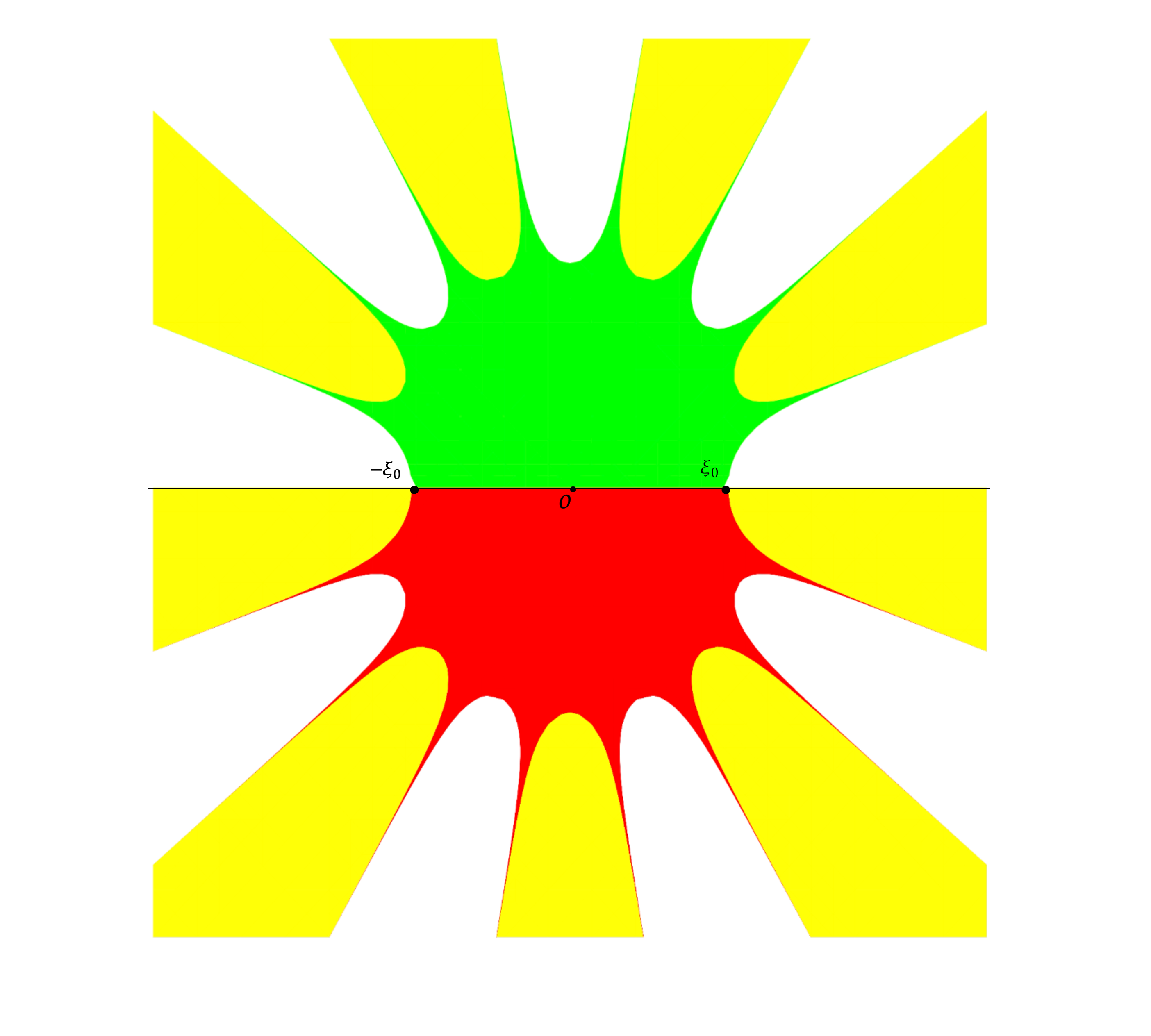
Figure 7: Signature of $\operatorname{Re}(i\theta)$. The green region: $\operatorname{Re}(i\theta)>0$ when $x<0$; The red region: $\operatorname{Re}(i\theta)>0$ when $x>0$; The yellow region: the overlapping region of red and green; The white region: $\operatorname{Re}(i\theta)<0$. Here we only plot the signatures of $\operatorname{Re}{(i\theta)}$ for $n=9$. Other odd $n$, the region plot looks very similar.

Note that

$$e^{-i\theta(z)\text{ ad }\sigma_{3}}v(z) =e^{-i\Theta(\xi)\text{ ad }\sigma_{3}}v(\xi)$$

$$=\begin{pmatrix}1-|R|^{2}&-\bar{R}e^{-2i\Theta}\\ Re^{2i\Theta}&1\end{pmatrix}$$

$$=\begin{pmatrix}1&-\bar{R}e^{-2i\Theta}\\ 0&1\end{pmatrix}\begin{pmatrix}1&0\\ Re^{2i\Theta}&1\end{pmatrix}.$$

We can deform the the contour $\{z\in\mathbb{R}:|z|>|\xi_{0}|\}$ as before and get the deformed contour as follows (see Fig.8): Fix a positive constant $\alpha<\frac{\pi}{n}$,

$$\Sigma_{0} =\{z\in\mathbb{R}:-\xi_{0}\leq z\leq\xi_{0}\},$$

$$\Sigma_{1} =\{z:z=\xi_{0}+\rho e^{i\alpha},\rho\in(0,\infty)\},$$

$$\Sigma_{2} =\{z:z=-\xi_{0}+\rho e^{-i\alpha},\rho\in(-\infty,0)\},$$

$$\Sigma_{3} =\{z:z=-\xi_{0}+\rho e^{i\alpha},\rho\in(-\infty,0)\},$$

$$\Sigma_{4} =\{z:z=\xi_{0}+\rho e^{-i\alpha},\rho\in(0,\infty)\},$$

and we define the regions as follows:

$$\Omega_{1} =\{z:z=\xi_{0}+\rho e^{i\phi},\rho\in(0,\infty),\phi\in(0,\alpha)\},$$

$$\Omega_{2} =\mathbb{C}^{+}\backslash(\Omega_{1}\cup\Omega_{3}),$$

$$\Omega_{3} =\{z:z=-\xi_{0}+\rho e^{-i\phi},\rho\in(-\infty,0),\phi\in(-\alpha,0)\},$$

$$\Omega_{4} =\{z:z=-\xi_{0}+\rho e^{i\phi},\rho\in(-\infty,0),\phi\in(0,\alpha)\},$$

$$\Omega_{5} =\mathbb{C}^{-}\backslash(\Omega_{4}\cup\Omega_{6}),$$

$$\Omega_{6} =\{z:z=\xi_{0}+\rho e^{i\phi},\rho\in(0,\infty),\phi\in(-\alpha,0)\}.$$

Figure 8: Contour for $\bar{\partial}$-RHP.

As before, set the original RHP as $m^{[1]}$ with jump $e^{-i\theta(z)\text{ ad }\sigma_{3}}v(z)$. After re-scaling and $\bar{\partial}$-lenses opening, we set $m^{[2]}(\xi)=m^{[1]}O(\gamma)$, where the lenses opening matrix is

$$O(\gamma)=\begin{cases}\begin{pmatrix}1&0\\ -E_{+}e^{2i\Theta(\gamma)}&1\end{pmatrix},\quad\gamma\in\Omega_{1}\cup\Omega_{3},\\ \begin{pmatrix}1&-E_{-}e^{-2i\Theta(\gamma)}\\ 0&1\end{pmatrix},\quad\gamma\in\Omega_{4}\cup\Omega_{6},\\ I,\quad\gamma\in\Omega_{2}\cup\Omega_{5},\end{cases}$$ (81)

where

$$E_{+}(\gamma) =\mathcal{K}(\phi)R\left((nt)^{-\frac{1}{n}}\xi\right)+(1-\mathcal{K}(\phi))R(\tilde{\xi}_{0}(nt)^{-\frac{1}{n}}),$$

$$E_{-} (\gamma)=\overline{E_{+}(\gamma)},$$

$$\gamma =\begin{cases}\xi_{0}+\rho e^{i\phi},\quad\text{if }\gamma\in\Omega_{1}\cup\Omega_{6},\\ -\xi_{0}+\rho e^{i\phi},\quad\text{if }\gamma\in\Omega_{3}\cup\Omega_{4},\end{cases}$$

$$\xi =\operatorname{Re}(\gamma),$$

$$\tilde{\xi}_{0} =\begin{cases}\xi_{0},\quad\text{if }\gamma\in\Omega_{1}\cup\Omega_{6},\\ -\xi_{0},\quad\text{if }\gamma\in\Omega_{3}\cup\Omega_{4}.\end{cases}$$

Now we arrive at the following $\bar{\partial}$-RHP:

Mixed $\bar{\partial}$-Riemann-Hilbert problem 11.1.

1. Looking for a 2 by 2 matrix-valued function $m^{[2]}$ such that

2. The RHP:

   (1.a) $m^{[2]}(\gamma)\in C^{1}(\mathbb{R}^{2}\backslash\Sigma)$ and $m^{[2]}(z)=I+\mathcal{O}(\gamma^{-1}),\gamma\rightarrow\infty$;

   (1.b) the jumps on $\Sigma_{1}$ and $\Sigma_{2}$ are $e^{-i\Theta(\xi)\text{ ad }\sigma_{3}}v_{+}$, and the jumps on $\Sigma_{3}$ and $\Sigma_{4}$ are $e^{-i\Theta(\xi)\text{ ad }\sigma_{3}}v_{-}$, where

   $$v_{=}\begin{pmatrix}1&\bar{R}\\ 0&1\end{pmatrix},\quad v_{+}=\begin{pmatrix}1&0\\ R&1\end{pmatrix}.$$

   The jump on $\Sigma_{0}$ is $e^{-i\Theta\text{ ad }\sigma_{3}}v((nt)^{-\frac{1}{n}}\xi),$, and the jumps on $\{z\in\mathbb{R}:|z|>|\xi_{0}|\}$ is $I$.

3. The $\bar{\partial}$-problem:

   For $z\in\mathbb{C}$, we have

   $$\bar{\partial}m^{[2]}(\xi)=m^{[2]}(\xi)\bar{\partial}O(\xi).$$ (82)

Again, we will need the following lemma in order to estimate errors from the $\bar{\partial}$-problem.

Lemma 11.2.

For $\gamma\in\Omega_{1,3,4,6}$, $\xi=\operatorname{Re}\gamma$,

$$|\bar{\partial}E_{\pm}(\gamma)|\leq(nt)^{-\frac{1}{n}}|(nt)^{-\frac{1}{n}}(\xi-\xi_{0})|^{-\frac{1}{2}}\|R\|_{H^{1,0}}+(nt)^{-\frac{1}{n}}|R^{\prime}((nt)^{-\frac{1}{n}}\xi)|.$$ (83)

Proof.

For brevity, we only prove for the region $\Omega_{1}$. Using the polar coordinates, we have

$$|\bar{\partial}E_{+}(\gamma)| =\left|\frac{ie^{i\phi}}{2\rho}\mathcal{K}^{\prime}(\phi)\left[R\left((nt)^{-\frac{1}{n}}\xi\right)-R(\xi_{0}(nt)^{-\frac{1}{n}})\right]+\mathcal{K}(\phi)R^{\prime}\left((nt)^{-\frac{1}{n}}\xi\right)(nt)^{-\frac{1}{n}}\right|$$

by Cauchy-Schwartz inequality

$$\leq\left|\frac{\|R\|_{H^{1,0}}|(nt)^{-\frac{1}{n}}\xi-\xi_{0}(nt)^{-\frac{1}{n}}|^{1/2}}{\gamma-\xi_{0}}\right|+(nt)^{-\frac{1}{n}}\left|R^{\prime}\left((nt)^{-\frac{1}{n}}\xi\right)\right|$$

$$\leq(nt)^{-\frac{1}{n}}|(nt)^{-\frac{1}{n}}(\xi-\xi_{0})|^{-\frac{1}{2}}\|R\|_{H^{1,0}}+(nt)^{-\frac{1}{n}}|R^{\prime}((nt)^{-\frac{1}{n}}\xi)|.$$

Similarly, we can prove for other regions. ∎

Next, consider a pure RHP $m^{[3]}$ which satisfies exactly the RHP part of $\bar{\partial}$-RHP($m^{[2]}$). $m^{[3]}$ can be approximated by the RHP corresponding to a special solution of the Painlevé II hierarchy. Since for $\gamma\in\Omega_{1}$,

$$\left|\left(R(\xi(nt)^{-\frac{1}{n}})-R(0)\right)e^{2i\Theta(\gamma)}\right|$$

$$\leq|\xi(nt)^{-\frac{2}{n}}|^{\frac{1}{2}}\|R\|_{H^{1,0}}e^{2\operatorname{Re}{i\Theta(\gamma)}}$$

$$\leq(nt)^{-\frac{1}{n}}|\operatorname{Re}\gamma|^{\frac{1}{2}}\|R\|_{H^{1,0}}e^{2\operatorname{Re}{i\Theta(\gamma)}},$$

it is evident that

$$\|Re^{2i\Theta}-R(0)e^{2i\Theta}\|_{L^{\infty}\cap L^{1}\cap L^{2}}\leq c(nt)^{-\frac{1}{n}}.$$ (84)

Let $m^{[4]}$ solves the RHP formed by replacing $R(\pm\xi_{0}(nt)^{-1/n})$ and its complex conjugate in the jumps of $m^{[3]}$ along $\Sigma_{k},k=1,2,3,4$ by $R(0)$ and $\bar{R}(0)$ respectively. Then, by the small norm theory, the errors between the corresponding potential is given by

$$error_{3,4} =\lim_{\gamma\rightarrow\infty}|\gamma(m^{[4]}_{12}-m^{[3]}_{12})|$$

$$\leq c\int_{\Sigma}|(R(\operatorname{Re}(s)(nt)^{-\frac{1}{n}})-R(0))e^{2i\Theta(s)}|ds$$

$$\leq c(nt)^{-\frac{1}{n}}.$$

Then since now the jumps are all analytic, we can perform an analytic deformation and arrive at the green contours as show in Fig.9. Let’s denote the new RHP by $m^{[5]}(\gamma)$, and we arrive at the following RHP:

Riemann-Hilbert problem 11.3.

Looking for a 2 by 2 matrix-valued function $m^{[5]}$ such that

1. $m^{[5]}$ is analytic off the contours $\cup_{k=1,2,3,4}\Sigma_{k}^{[5]}$;

2. $m^{[5]}_{+}=m^{[5]}_{-}v^{[5]},\quad z\in\cup_{k=1,2,3,4}\Sigma_{k}^{[5]},$ where

   $$v^{[5]}=\begin{cases}\begin{pmatrix}1&0\\ R(0)e^{2i\Theta(\gamma)}&1\end{pmatrix},\quad\gamma\in\Sigma_{1}^{[5]}\cup\Sigma_{2}^{[5]},\\ \begin{pmatrix}1&\bar{R}(0)e^{-2i\Theta(\gamma)}\\ 0&1\end{pmatrix},\quad\gamma\in\Sigma_{3}^{[5]}\cup\Sigma_{4}^{[5]}.\end{cases}$$

Here the new contours (see Fig.9) are

$$\Sigma_{1}^{[5]} =\{z:z=\rho e^{i\alpha},\rho\in(0,\infty)\},$$

$$\Sigma_{2}^{[5]} =\{z:z=\rho e^{-i\alpha},\rho\in(-\infty,0)\},$$

$$\Sigma_{3}^{[5]} =\{z:z=\rho e^{i\alpha},\rho\in(-\infty,0)\},$$

$$\Sigma_{4}^{[5]} =\{z:z=\rho e^{-i\alpha},\rho\in(0,\infty)\}.$$

Figure 9: Contour for $m^{[4]}$(Green part).

Then according to the previous subsection, the $(1,2)$ entry of the solution $m^{[5]}$, similarly the solution $m^{[4]}$, is the solution to the Painlevé II hierarchy, i.e.,

$$m^{[4]}_{12}(\gamma)=m^{[5]}_{12}(\gamma),$$ (85)

Hence we have $P^{II}_{k}(s)=\lim_{\gamma\rightarrow\infty}\gamma m^{[5]}_{12}$ where $P^{II}_{k}$ solves the $k^{th}$ equation in the Painlevé II hierarchy, where $k=\frac{n-1}{2}$.

Now let’s consider the error generated from the $\bar{\partial}$-extension. Recall that the error $E$ satisfies a pure $\bar{\partial}$-problem:

$$\bar{\partial}E =EW,$$

$$W =m^{[3]}\bar{\partial}O(m^{[3]})^{-1}.$$

As before, the $\bar{\partial}$-equation is equivalent to an integral equation which reads

$$E(z)=I+\frac{1}{\pi}\int_{\mathbb{C}}\frac{E(s)W(s)}{z-s}\text{d}A(s)=I+\mathcal{K}(E).$$

As before, we can show that the resolvent always exists for large $t$. So we only need to estimate the true error which is: $\lim_{z\rightarrow\infty}z(E-I)$. In fact, we have

$$\lim_{z\rightarrow\infty}|z(E-I)| =|\int_{\mathbb{C}}EWds|$$

$$\leq c\|E\|_{\infty}\int_{\Omega}|\bar{\partial}O|ds.$$

For the sake of simplicity, we only estimate the integral on the right hand side in the region of the top right corner. Note there is only one entry which is nonzero in $\bar{\partial}O$, which is one of the $E_{\pm}$ and we split the integral into two parts in the obvious way, i.e.,

$$\int_{\Omega}|\bar{\partial}O|ds \leq I_{1}+I_{2}$$

$$=\int_{\Omega}(nt)^{-\frac{1}{2n}}|\operatorname{Re}{s}-\xi_{0}|\|R\|_{H^{1,0}}e^{2\operatorname{Re}{i\Theta(s)}}ds$$

$$+\int_{\Omega}(nt)^{-\frac{1}{nt}}|R^{\prime}((nt)^{-\frac{1}{n}}s)|e^{2\operatorname{Re}{i\Theta(s)}}ds.$$

As we know from previous sections, $e^{\operatorname{Re}{2i\Theta(s)}}\leq ce^{-2|\Theta^{\prime\prime}(\xi_{0})|uv}$ in the region $\{z=u+iv:u>\xi_{0},0<v<\alpha u\}$ for some small $\alpha$ , where $s=u+iv+\xi_{0}$. Then we have

$$I_{1} \leq(nt)^{-\frac{1}{2n}}\int_{\Omega}|\operatorname{Re}{s}-\xi_{0}|^{-1/2}e^{-cuv}dudv$$

$$\leq(nt)^{-\frac{1}{2n}}\int_{0}^{\infty}\int_{0}^{\alpha u}u^{-1/2}e^{-cuv}dudv$$

$$\leq C(nt)^{-\frac{1}{2n}}\int_{0}^{\infty}\frac{1-e^{-2\alpha|\Theta^{\prime\prime}(\xi_{0})|}}{u^{3/2}}du$$

$$=\mathcal{O}\left((nt)^{-\frac{1}{2n}}\right),$$

and

$$I_{2} \leq(nt)^{-\frac{1}{n}}\int|R^{\prime}((nt)^{-\frac{1}{2n}}\operatorname{Re}{s})|e^{-cuv}dudv$$

by Cauchy-Schwartz inequality

$$\leq(nt)^{-\frac{1}{n}}\|R\|_{H^{1,0}}\int_{0}^{\infty}(\int_{\alpha v}^{\infty}e^{-2cuv}du)^{1/2}dv$$

$$\leq(nt)^{-\frac{1}{n}}\|R\|_{H^{1,0}}\int_{0}^{\infty}\frac{e^{-c\alpha v^{2}}}{\sqrt{2\alpha cv}}dc$$

$$=\mathcal{O}((nt)^{-\frac{1}{n}}).$$

Thus, we arrive at

$$\bar{\partial}\text{Error}=\mathcal{O}((nt)^{-\frac{1}{2n}}).$$ (86)

And we undo all the deformations, we obtain

$$m^{[1]}((nt)^{-\frac{1}{n}}\gamma) =m^{[2]}(\gamma)O^{-1}(\gamma)$$

$$=(1+\frac{\mathcal{O}{(t^{\frac{1}{2n}})}}{\gamma})m^{[3]}(\gamma)O^{-1}(\gamma)$$

$$=(1+\frac{\mathcal{O}{(t^{\frac{1}{2n}})}}{\gamma})(1+\frac{\mathcal{O}{(t^{\frac{1}{2n}})}}{\gamma})m^{[4]}(\gamma)O^{-1}(\gamma)$$

$$=(1+\frac{\mathcal{O}{(t^{\frac{1}{2n}})}}{\gamma})(1+\frac{\mathcal{O}{(t^{\frac{1}{2n}})}}{\gamma})m^{[5]}(\gamma)O^{-1}(\gamma).$$

It can also be rewritten in terms of the variable $z$:

$$m^{[1]}(z)=\left(1+\frac{\mathcal{O}{(t^{-1/(2n)}})}{z(nt)^{1/n}}\right)m^{[5]}((nt)^{1/n}z)+\mathcal{O}{(z^{-2})},\quad z\rightarrow\infty.$$

Since $m^{[5]}$ corresponds to the RHP for the Painlevé II hierarchy, we have

$$m^{[5]}(\gamma)=I+\frac{m_{1}^{[5]}(s)}{\gamma}+\mathcal{O}(\gamma^{-1}),$$

where $\gamma=z(nt)^{1/n}$.

Thus,

$$m^{[1]}(z) =\left(1+\frac{\mathcal{O}{(t^{-\frac{1}{2n}})}}{z(nt)^{1/n}}\right)\left(1+\frac{m_{1}^{[5]}(s)}{z(nt)^{1/n}}+\mathcal{O}(z^{-2})\right)$$

$$=I+\frac{m_{1}^{[5]}(s)}{z(nt)^{1/n}}+\frac{\mathcal{O}{(t^{-\frac{1}{2n}})}}{z(nt)^{1/n}}+\mathcal{O}(z^{-2}).$$

Since $m_{1}^{[5]}(s)$ is connected to solutions of the Painlevé II hierarchy, we conclude that

$$q(x,t) =\lim_{z\rightarrow\infty}z(m^{[1]}-I)$$

$$=(nt)^{-\frac{1}{n}}u_{n}(x(nt)^{-\frac{1}{n}})+\mathcal{O}{(t^{-\frac{3}{2n}})},$$

where $u_{n}$ solves the $\frac{n-1}{2}$th equation of the Painlevé II hierarchy. The odd integer $n$ corresponds to the $\frac{n-1}{2}$th member in the mKdV hierarchy.

Remark 11.4.

As for the asymptotics for the Painlevé II equation, we refer the readers to the classical book [20]. There are also some recent works related to Painlevé II hierarchy, see for example [30],[9],[6].

References

[1]
M. A. Ablowitz and P. A. Clarkson.
Solitons, Nonlinear Evolution Equations and Inverse Scattering.
London Mathematical Society Lecture Note Series. Cambridge University
Press, 1991.
[2]
M. J. Ablowitz and H. Segur.
Exact Linearization of a Painlevé Transcendent.
Phys. Rev. Lett., 38:1103–1106, May 1977.
[3]
R. Beals and R. R. Coifman.
Scattering and inverse scattering for first order systems.
Communications on Pure and Applied Mathematics, 37(1):39–90,
1984.
[4]
R. Beals, P. Deift, and C. Tomei.
Direct and inverse scattering on the line.
American Mathematical Society, 1988.
[5]
M. Borghese, R. Jenkins, and K. D.-R. McLaughlin.
Long time asymptotic behavior of the focusing nonlinear
Schrödinger equation.
Annales de l’Institut Henri Poincaré C, Analyse non
linéaire, 35(4):887–920, 2018.
[6]
M. Cafasso, T. Claeys, and M. Girotti.
Fredholm Determinant Solutions of the Painlevé II Hierarchy and
Gap Probabilities of Determinantal Point Processes.
International Mathematics Research Notices, 2021(4):2437–2478,
09 2019.
[7]
G. Chen and J. Liu.
Long-time asymptotics of the modified KdV equation in weighted
Sobolev spaces, 2019.
arXiv: 1903.03855.
[8]
G. Chen, J. Liu, and B. Lu.
Long-time asymptotics and stability for the sine-Gordon equation,
2020.
arXiv: 2009.04260.
[9]
T. Claeys, I. Krasovsky, and A. Its.
Higher-order analogues of the Tracy-Widom distribution and the
Painlevé II hierarchy.
Communications on Pure and Applied Mathematics, 63(3):362–412,
2010.
[10]
P. Clarkson, N. Joshi, and M. Mazzocco.
The Lax pair for the mKdV hierarchy.
Théories Asymptotiques Et équations De Painlevé, Sémin.
Congr, 14:53–64, 01 2006.
[11]
P. A. Clarkson, N. Joshi, and A. Pickering.
Bäcklund transformations for the second Painlevé hierarchy: a
modified truncation approach.
Inverse Problems, 15(1):175–187, jan 1999.
[12]
P. Deift, T. Kriecherbauer, and K.-R. McLaughlin.
New results on the equilibrium measure for logarithmic potentials in
the presence of an external field.
Journal of approximation theory, 95(3):388–475, 1998.
[13]
P. Deift, T. Kriecherbauer, K. T.-R. McLaughlin, S. Venakides, and X. Zhou.
Strong asymptotics of orthogonal polynomials with respect to
exponential weights.
Communications on Pure and Applied Mathematics,
52(12):1491–1552, 1999.
[14]
P. Deift and X. Zhou.