Multidimensional Persistence Module Classification via Lattice-Theoretic Convolutions

Abstract

Multiparameter persistent homology has been largely neglected as an input to machine learning algorithms. We consider the use of lattice-based convolutional neural network layers as a tool for the analysis of features arising from multiparameter persistence modules. We find that these show promise as an alternative to convolutions for the classification of multidimensional persistence modules.

1 Introduction

Persistent homology has the ability to discern both the global topology [10] and local geometry [5] of finite metric spaces (e.g. embedded weighted graphs, point clouds in $\mathbb{R}^{d}$) making it a befitting feature for the purposes of training a neural network. Single-dimensional homological persistence has drawn recent attention in deep learning [12, 21, 3]. This is, in part, due to a wide range of efficient software libraries [19, 11, 2] for computing persistent homology, as well as a growing cookbook of recipes for featurizing barcodes from single dimensional persistence, including persistence images [1], persistence landscapes [4], and more exotic methods [13].

Multidimensional persistence generalizes single-dimensional persistent homology in order to tackle filtrations parameterized in multiple dimensions. Unfortunately, there is no complete compact barcode-like characterization of multidimensional persistence modules [7]. We must make do with incomplete invariants. There are various algebraic invariants; in this paper we will use the Hilbert function and the multi-graded Betti numbers, both of which are $\mathbb{N}$-valued functions on the parameter space. The Hilbert function is nothing more than the pointwise (topological) Betti numbers, and the multi-graded Betti numbers have a geometric interpretation in terms of births and deaths [14]. The rank invariant, another invariant, is shown to be complete in the case of single dimensional persistence [7]; due to its difficulty to compute it is not considered here.

Multidimensional persistence suffers two hindrances to its usefulness in machine learning. First, software for computing multidimensional persistence is scarce. To the authors’ knowledge, RIVET is the only available software for computing multidimensional persistence [16]; RIVET specializes to $2$-dimensional persistence and is focused on interactive visualization rather than machine-interpretable output. Second, there has been only very recent and preliminary activity [23, 8] focusing on extraction of suitable features for multidimensional persistent homology. A full-fledged deep learning pipeline for multidimensional persistence waits in the wings.

We hope to ignite further interest in filling both of these gaps. In this paper, we propose a naive featurization of multidimensional persistence modules based on the aforementioned invariants, and design an architecture for classifying these persistence modules. This architecture employs a lattice-theoretic notion of convolution, thereby respecting the order relation of the parameters of the persistence module. We implement our model and compare the performance of our proposed lattice-convolutional architecture with a (simplified) standard convolutional architecture.

Related work

Very recent advances have been made to featurize multidimensional persistence modules via landscapes [23] and images [8]. Our naive approach at featurizing $2$-dimensional persistence modules has the advantage of being readily computable with existing software [16]. Persistence modules supported on lattices are a popular object of study as of late. By leveraging Möbius inversion, these persistence modules are shown to generate a stable persistence diagram [17] as well as factor through a convenient category with pseudo-inverses [15].

2 Backgound

Space constraints require that this section be laconic. For a primer on persistent homology, see [10, 6]; for multiparameter persistent homology, see [16]. An introduction to lattices may be found in [9].

2.1 Rips complexes and persistent homology

Let $(\mathcal{M},d)$ be a finite metric space. The Vietoris-Rips complex of $\mathcal{M}$ at scale $r$ is the abstract simplicial complex $\text{Rips}_{r}(\mathcal{M})$ whose simplices are subsets of $\mathcal{M}$ of diameter at most $r$. There is a natural inclusion $\text{Rips}_{r}(\mathcal{M})\to\text{Rips}_{r^{\prime}}(\mathcal{M})$ for $r\leq r^{\prime}$.

Applying the simplicial homology functor (with coefficients in a field $k$) $H_{i}$ to $\text{Rips}_{r}(\mathcal{M})$ produces a sequence of vector spaces $PH_{i}(r)$. The inclusions $\text{Rips}_{r}(\mathcal{M})\to\text{Rips}_{r^{\prime}}(\mathcal{M})$ induce maps $PH_{i}(r)\to PH_{i}(r^{\prime})$, producing the data of a persistence module. This structure can be compactly described as a functor from $\mathbb{R}$, viewed as a category via its standard order structure, to the category $\operatorname{\mathbf{Vect}}_{k}$ of vector spaces over $k$. The simplicity of the category $\mathbb{R}$ gives these persistence modules simple structure: they decompose as direct sums of interval modules $I_{[a,b)}$, which have $I_{[a,b)}(r)=k$ for $a\leq r<b$ and zero otherwise. The maps are the identity where possible and the zero map otherwise.

2.2 Multiparameter persistence

The Rips construction produces a filtration of simplicial complexes from a finite metric space; it is natural to consider the behavior of the homology functor over a pair of coherent filtrations. Consider a finite metric space $(\mathcal{M},d)$ and a filtration function $\rho:\mathcal{M}\to\mathbb{R}$. This data specifies a bifiltration of simplicial complexes given by

$$\mathbb{X}_{r,t}=\text{Rips}_{r}\{x\in\mathcal{M}\mid\rho(x)\leq t\}.$$

There is a natural inclusion $\mathbb{X}_{r,t}\hookrightarrow\mathbb{X}_{r^{\prime},t^{\prime}}$ whenever $(r,t)\leq(r^{\prime},t^{\prime})$ in the lattice $\mathbb{R}\times\mathbb{R}$. Composing with the homology functor produces a 2-parameter persistence module

$$PH_{i}:\mathbb{R}_{+}\times\mathbb{R}\to\operatorname{\mathbf{Vect}};\quad(r,t)\mapsto H_{i}(X_{r,t}).$$

While there does not exist a complete discrete invariant for $PH_{i}$, we can extract meaningful features. Two particularly informative types of features are the Hilbert function

$$\text{Hilb}:\mathbb{R}_{+}\times\mathbb{R}\to\mathbb{Z}_{+};\quad(r,t)\mapsto\dim(PH_{i}(r,t)),$$

and the multi-graded Betti numbers $\xi_{j}:\mathbb{R}_{+}\times\mathbb{R}\to\mathbb{Z}_{+}$, for $j=0,1,2$. For $PH_{i}$ as above, the Hilbert function counts the number of connected components ($i=0$), cycles ($i=1$), or higher dimensional voids ($i>1$) of the complex $\mathbb{X}_{r,t}$ at each $(r,t)\in\mathbb{R}_{+}\times\mathbb{R}$. The multi-graded Betti numbers, on the other hand, capture information about births and deaths of homology classes.

2.3 Lattice-theoretic signal processing

Classical signal processing proceeds by constructing filters for space- or time-indexed signals using convolutional operators. These implicitly rely on the algebraic properties of the underlying space, in particular the existence of well-behaved translation operators. This fact is exploited in the general framework of algebraic signal processing [22] and extended to more general domains by the theory of graph signal processing [18]. We here describe a similar extension to signals on a finite lattice proposed in [20].

A lattice $L$ is a partially ordered set in which every pair of elements $x,y$ has a greatest lower bound (the meet $x\wedge y$) and a least upper bound (the join $x\vee y$). These operations and their properties produce an algebraic characterization of lattices; the ordering can be recovered from the algebra and vice versa. The key insight of [20] is that the meet and join operations on a lattice define two “shift operators” that can be exploited to define convolutional filters for signals on a lattice.

That is, for two signals $f,g:L\to\mathbb{R}$, where $L$ is a lattice, we define

$$(f*_{\wedge}g)(x)=\sum_{a\in L}f(x\wedge a)g(a)\;\;\text{and}\;\;(f*_{\vee}g)(x)=\sum_{a\in L}f(x\vee a)g(a).$$

A nice class of examples of lattices are given by the sets $\mathbb{R}^{n}$ viewed as partially ordered sets, with the ordering $(x_{1},\ldots,x_{n})\leq(y_{1},\ldots,y_{n})$ whenever $x_{i}\leq y_{i}$ for all $1\leq i\leq n$. These are, of course, the indexing sets for persistent homology, suggesting that lattice convolutions over $\mathbb{R}^{n}$ or its finite sublattices may be useful in processing data coming from multiparameter persistence computations.

3 Lattice Convolutional Neural Networks

Convolutions over $\mathbb{R}^{2}$ (with its abelian group structure) have served as an easily parameterized and efficient set of linear operations adapted to the structure of images. Their extreme utility in computer vision problems is owed to the translation equivariance properties of images: humans naturally recognize an image translated via an additive reparameterization as equivalent to the original.

The data of a multidimensional persistence module is also indexed by $\mathbb{R}^{n}$ or a regular finite subset thereof, but its natural algebraic structure is not that of an abelian group. Rather, with its partial order structure, the indexing set is a lattice. In processing signals associated with a persistence module, it may be useful to take this structure into account rather than imposing the abelian group structure implied by standard convolutions.

To this end, we construct a lattice convolution-based neural network layer suitable for use with features originating from multidimensional persistence modules. To the authors’ knowledge, such an architecture has not previously been described, although a special case (where the underlying lattice is a power set) has been implemented in [24]. We specialize the convolutions described in Section 2.3 to the particular case of regular finite sublattices of $\mathbb{R}^{2}$. These may be represented (up to isomorphism) as $L=[m]\times[n]$, where $[n]$ is the ordered set $\{0,1,\dots,n\}$. The meet and join operations are easily computed elementwise:

$$(r,t)\wedge(r^{\prime},t^{\prime})=(\min(r,r^{\prime}),\min(t,t^{\prime}));\quad(r,t)\vee(r^{\prime},t^{\prime})=(\max(r,r^{\prime}),\max(t,t^{\prime})).$$

A lattice convolution layer takes as input an $N_{\text{in}}$-dimensional signal $f:[m]\times[n]\to\mathbb{R}^{N_{\text{in}}}$ and outputs an $N_{\text{out}}$-dimensional signal $[m]\times[n]\to\mathbb{R}^{N_{\text{out}}}$. The layer’s parameters are given by a function $g:[m]\times[n]\to\mathbb{R}^{N_{\text{out}}\times N_{\text{in}}}$. If we label the entries of $f(x,y)$ by $f_{i}$ and the entries of $g(x,y)$ by $g^{i}_{j}$, the layer then acts by

$$\text{MeetConv}(f)(x,y)^{j}=\sum_{i}(f_{i}\ast_{\wedge}g^{i}_{j})(x,y)=\sum_{i}\sum_{(a,b)\in[m]\times[n]}f_{i}(x\wedge a,y\wedge b)g^{i}_{j}(a,b)$$

in the case of convolution with respect to the meet operation, and

$$\text{JoinConv}(f)(x,y)^{j}=\sum_{i}(f_{i}\ast_{\vee}g^{i}_{j})(x,y)=\sum_{i}\sum_{(a,b)\in[m]\times[n]}f_{i}(x\vee a,y\vee b)g^{i}_{j}(a,b)$$

in the case of convolution with respect to the join operation.

Remark

Traditional convolutional neural networks are useful in part because the convolution kernels (here the functions $g$) can have very small support, reducing the number of parameters that must be learned. In the standard convolutional setting, these kernels are implicitly supported in a neighborhood of the origin, but the location of the kernel is not usually explicitly specified. In the lattice setting, we do need to specify where the kernel resides. In the abelian group case, the kernel is supported near the identity, and similarly, when we treat our domain as a lattice, the kernel should be supported near the neutral element of the operation. That is, for a meet convolution, $g$ should be supported at the maximum $(m,n)$, and for a join convolution, $g$ should be supported at the minimum $(0,0)$. This ensures that the convolution operators are capable of preserving information at every point of the space. For instance, if $g(0,0)\neq 0$, then $(f\ast_{\vee}g)(x,y)$ is a sum of terms including $f(x,y)g(0,0)$, so all information from one layer can be passed to the next layer. A bit more is necessary to avoid degenerate convolutions. A kernel supported in a geometrically small neighborhood of the neutral element results in trivial receptive fields for most neurons. For example, if $(x,y)$ is greater than the maximal element of the support of $g$, $(f\ast_{\vee}g)(x,y)$ is simply a scalar multiple of $f(x,y)$. As a result, we hypothesize that the appropriate support sets for lattice-convolutional kernels are evenly-spaced sublattices including both $(0,0)$ and $(m,n)$.

4 Experiments

We use a portion of the Princeton ModelNet dataset [25] as a source of finite metric spaces. This dataset consists of hundreds of 3-dimensional CAD models representing objects from 10 classes. We sample points from the 3D models to produce finite metric spaces embedded in $\mathbb{R}^{3}$. We then compute the corresponding multidimensional persistence modules, from which we produce features used as an input to a convolutional neural net classifier.

The pipline thus begins with a 3D polyhedral model, of which $3000$ vertices are sampled to produce a point cloud in $\mathbb{R}^{3}$. This point cloud then produces a bifiltered simplicial complex, whose degree-$0$ persistent homology we calculate using RIVET [16], sampled at a discrete grid of $40\times 40$ points, producing lattice-indexed signals given by the Hilbert function and the multi-graded Betti numbers $\xi_{0},\xi_{1},\xi_{2}$; four features in total. These are then passed to the classifier, which produces a class prediction, in this case one of 10 possible household objects.

As the filter function on these data sets, we use the codensity function

$$\rho_{\text{codense}}(x;k)=\left(\frac{1}{k}\sum_{y\in N_{k}(x)}d(x,y)\right)^{-1},$$

where $N_{k}(x)$ is the set of the $k$ nearest neighbors to $x$; we select $k=100$.

Remark

The name codensity is appropriate because the points in the densest regions of $\mathcal{M}$ appear earlier in the filtration. A folk theorem is that the 2-parameter persistent homology of a Rips/codensity bifiltration is stable (w.r.t. interleaving distance) under non-Hausdorff noise (e.g. adding or removing a small number of point samples).

We compare the performance of two convolutional networks on this classification task. One uses the lattice-convolution based layers described in Section 3, and the other uses standard convolutional layers. Each has three convolutional layers followed by two fully connected layers. The lattice-based convolution layers are of the form $\alpha\cdot\text{MeetConv}(x)+(1-\alpha)\cdot\text{JoinConv}(x)$ for a hyperparameter $\alpha\in[0,1]$. We set $\alpha=\frac{1}{2}$. All convolution kernels have dimension $4\times 4$, hidden convolution layers have 16 features, and the final convolution layer has 8 features. The first two convolution layers are followed by max-pooling layers with a $2\times 2$ kernel. For the lattice convolutional layers, the support of the kernel lay in an evenly spaced $4\times 4$ grid of points in $[m]\times[n]$, while the standard convolutional layers had a traditional contiguously supported kernel. The inner fully connected layer has 32 features. We use a cross entropy loss function with a softmax in the final layer. The lattice-based convolutional architecture is summarized in Figure 1. The networks are trained using the Adam gradient algorithm with learning rate $2\times 10^{-4}$ for 300 epochs. We reserve 10% of the data for testing. Results are shown in Figure 2.

The lattice convolutional network slightly underperforms the standard convolutional classifier. This is somewhat disappointing, and perhaps indicates that the relevant information encoded in degree-0 persistent homology is best captured with a geometric notion of locality in $\mathbb{R}^{2}$. This work has by no means exhausted the possibilities for lattice convolutions in multidimensional persistence, but does suggest circumspection in evaluating their future use.

5 Discussion

Our proposed featurization for persistence modules is rather naive, but well adapted to the use of lattice convolutions as a data processing method. The lattice convolutional neural network shows promise as a method for classifying features arising from a multiparameter persistence module. The algebraic perspective on partially ordered sets, exemplified by lattices, may also offer approaches to featurizing more complex invariants of persistence modules. In particular, the incidence algebra may offer a natural way to represent the rank invariant [7] in a way amenable to convolution-like operations. We hope with these brief experiments to inspire further work on featurizing multidimensional persistence for use in machine learning algorithms.

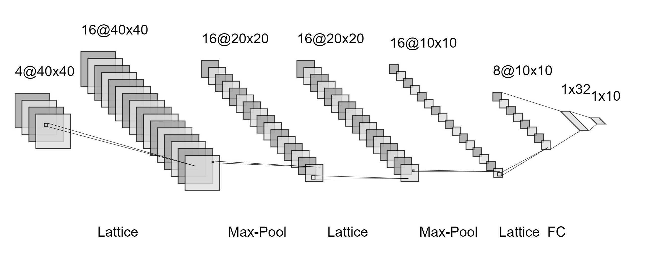
Figure 1: The architecture of our lattice-based convolutional neural network.

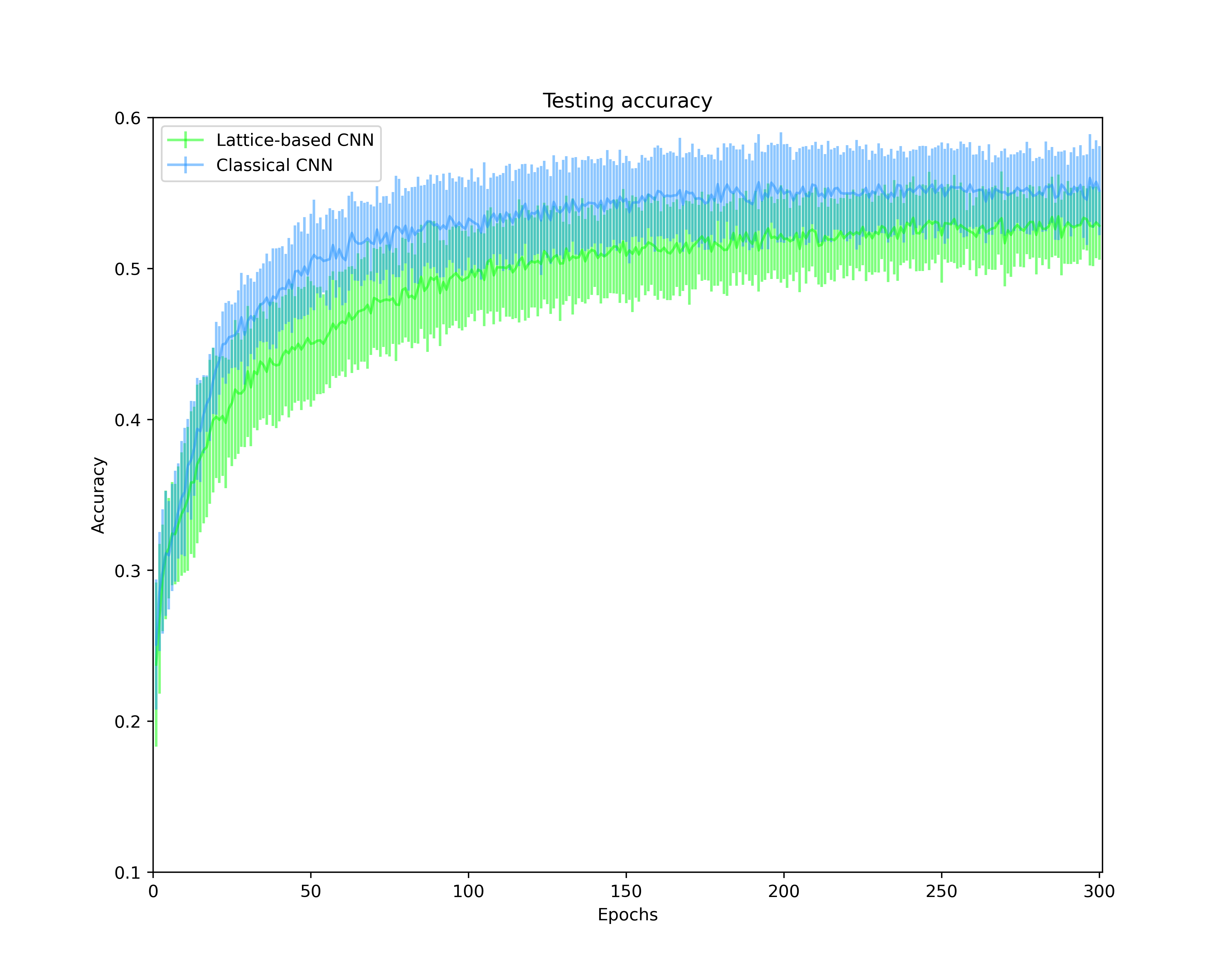
Figure 2: Comparison learning curves for the lattice neural network and standard convolutional neural network.

References

- [1] Henry Adams, Tegan Emerson, Michael Kirby, Rachel Neville, Chris Peterson, Patrick Shipman, Sofya Chepushtanova, Eric Hanson, Francis Motta, and Lori Ziegelmeier. Persistence Images: A Stable Vector Representation of Persistent Homology. Journal of Machine Learning Research, 18, 2017.
- [2] Ulrich Bauer. Ripser: Efficient computation of Vietoris-Rips persistence barcodes. arXiv:1908.02518 [cs, math], August 2019.
- [3] Rickard Brüel-Gabrielsson, Bradley J. Nelson, Anjan Dwaraknath, Primoz Skraba, Leonidas J. Guibas, and Gunnar Carlsson. A Topology Layer for Machine Learning. arXiv:1905.12200 [cs, math, stat], April 2020.
- [4] Peter Bubenik. Statistical Topological Data Analysis using Persistence Landscapes. Journal of Machine Learning Research, 16, 2015.
- [5] Peter Bubenik, Michael Hull, Dhruv Patel, and Benjamin Whittle. Persistent homology detects curvature. Inverse Problems, 36(2):025008, January 2020.
- [6] Gunnar Carlsson. Topology and data. Bulletin of the American Mathematical Society, 46:255–308, 2009.
- [7] Gunnar Carlsson and Afra Zomorodian. The Theory of Multidimensional Persistence. Discrete & Computational Geometry, 42(1):71–93, July 2009.
- [8] Mathieu Carrière and Andrew Blumberg. Multiparameter persistence image for topological machine learning. Advances in Neural Information Processing Systems, 33, 2020.
- [9] Brian A Davey and Hilary A Priestley. Introduction to lattices and order. Cambridge University Press, 2002.
- [10] Robert Ghrist. Barcodes: The persistent topology of data. Bulletin of the American Mathematical Society, 45:61–75, 2008.
- [11] Gregory Henselman and Robert Ghrist. Matroid filtrations and computational persistent homology. arXiv:1606.00199 [math], October 2017.
- [12] Christoph Hofer, Roland Kwitt, Marc Niethammer, and Andreas Uhl. Deep learning with topological signatures. In I. Guyon, U. V. Luxburg, S. Bengio, H. Wallach, R. Fergus, S. Vishwanathan, and R. Garnett, editors, Advances in Neural Information Processing Systems 30, pages 1634–1644. Curran Associates, Inc., 2017.
- [13] Sara Kališnik. Tropical Coordinates on the Space of Persistence Barcodes. Foundations of Computational Mathematics, 19(1):101–129, February 2019.
- [14] Kevin P. Knudson. A refinement of multi-dimensional persistence. Homology, Homotopy and Applications, 10(1):259–281, 2008.
- [15] Sanjeevi Krishnan and Crichton Ogle. Invertibility in category representations. pages 1–16.
- [16] Michael Lesnick and Matthew Wright. Interactive visualization of 2-d persistence modules. arXiv:1512.00180 [cs, math], December 2015.
- [17] Alexander McCleary and Amit Patel. Edit Distance and Persistence Diagrams Over Lattices. pages 1–17, 2020.
- [18] A. Ortega, P. Frossard, J. Kovačević, J. M. F. Moura, and P. Vandergheynst. Graph signal processing: Overview, challenges, and applications. Proceedings of the IEEE, 106(5):808–828, May 2018.
- [19] Nina Otter, Mason A. Porter, Ulrike Tillmann, Peter Grindrod, and Heather A. Harrington. A roadmap for the computation of persistent homology. EPJ Data Science, 6(1):17, August 2017.
- [20] Markus Pueschel. A discrete signal processing framework for meet/join lattices with applications to hypergraphs and trees. May 2019.
- [21] Chi Seng Pun, Kelin Xia, and Si Xian Lee. Persistent-Homology-based Machine Learning and its Applications – A Survey. arXiv:1811.00252 [math], November 2018.
- [22] Markus Puschel and JosÉ M. F. Moura. Algebraic Signal Processing Theory: Foundation and 1-D Time. IEEE Transactions on Signal Processing, 56(8):3572–3585, August 2008.
- [23] Oliver Vipond. Multiparameter persistence landscapes. Journal of Machine Learning Research, 21(61):1–38, 2020.
- [24] Chris Wendler, Markus Püschel, and Dan Alistarh. Powerset Convolutional Neural Networks. In H. Wallach, H. Larochelle, A. Beygelzimer, F. d\textquotesingle Alché-Buc, E. Fox, and R. Garnett, editors, Advances in Neural Information Processing Systems 32, pages 929–940. Curran Associates, Inc., 2019.
- [25] Zhirong Wu, Shuran Song, Aditya Khosla, Fisher Yu, Linguang Zhang, Xiaoou Tang, and Jianxiong Xiao. 3D ShapeNets: A deep representation for volumetric shapes. In 2015 IEEE Conference on Computer Vision and Pattern Recognition (CVPR), pages 1912–1920, Boston, MA, USA, June 2015. IEEE.