Preserving general physical properties in model reduction of dynamical systems via constrained-optimization projection

Alexander Schein schein@mhpc.mw.tum.de Kevin T. Carlberg ktcarlb@uw.edu Matthew J. Zahr mzahr@nd.edu Technical University of Munich Sandia National Laboratories University of Washington University of Notre Dame
Abstract

Model-reduction techniques aim to reduce the computational complexity of simulating dynamical systems by applying a (Petrov–)Galerkin projection process that enforces the dynamics to evolve in a low-dimensional subspace of the original state space. Frequently, the resulting reduced-order model (ROM) violates intrinsic physical properties of the original full-order model (FOM) (e.g., global conservation, Lagrangian structure, state-variable bounds) because the projection process does not generally ensure preservation of these properties. However, in many applications, ensuring the ROM preserves such intrinsic properties can enable the ROM to retain physical meaning and lead to improved accuracy and stability properties. In this work, we present a general constrained-optimization formulation for projection-based model reduction that can be used as a template to enforce the ROM to satisfy specific properties on the kinematics and dynamics. We introduce constrained-optimization formulations at both the time-continuous (i.e., ODE) level, which leads to a constrained Galerkin projection, and at the time-discrete level, which leads to a least-squares Petrov–Galerkin (LSPG) projection, in the context of linear multistep schemes. We demonstrate the ability of the proposed formulations to equip ROMs with desired properties such as global energy conservation and bounds on the total variation.

keywords:
projection-based model reduction , Galerkin projection , least-squares Petrov–Galerkin projection , constrained optimization

1 Introduction

Serving as a bridge to overcome the prohibitive computational cost of simulating large-scale, parameterized dynamical systems in time-critical scenarios, projection-based model reduction has gained popularity and yielded successes across problems in many applications, including fluid dynamics, structural dynamics, and reacting flows. In the context of proper orthogonal decomposition (POD) [26] or reduced-basis method [25] approaches, a computationally costly offline stage is first executed in which the parameterized dynamical system, or full-order model (FOM), is simulated at multiple parameter instances. Then, the state snapshots arising from these training simulations are employed to construct a low-dimensional affine trial subspace of the original state space; recent approaches have also investigated constructing low-dimension nonlinear trial manifolds [18] from these snapshots. A parameterized dynamical system of lower dimension, called the reduced-order model (ROM) is computed by performing a (Petrov–)Galerkin projection process of the original dynamical system onto this subspace; as a result, the ROM’s solution is restricted to evolve in the low-dimensional trial subspace. If the FOM operators are nonlinear in the state or non-affine in the parameters, then an additional ‘hyper-reduction’ approximation is required to ensure the resulting ROM simulation incurs an operation count that is independent of the FOM state-space dimension. Computational-cost savings are achieved in the online stage by simulating the low-cost ROM at new parameter instances.

The ROM approximation typically does not preserve important intrisic properties of the dynamical system, e.g., global conservation and hyperbolicity in the context of (semi-discretized) conservation laws [8] and energy conservation in the context of solid dynamics [3, 12]. Failure of the ROM to preserve these properties not only raises questions about the physical interpretability of the resulting solution, it also has been attributed to large state-space errors and lack of stability [9], which has motivated research on structure-preserving model reduction for different classes of dynamical systems. One class of such approaches derives governing equations for the ROM in a manner that preserves the structure of the original dynamical system, for example by preserving Lagrangian structure [9, 16], the principle of virtual work [12, 13], (Port-)Hamilton structure [24, 1, 23], the principle of mass conservation [19], or positivity of contact forces in adhesion-free normal contact [4]. Researchers have pursued several works on structure-preserving model reduction in computational fluid dynamics. Refs. [29, 2] investigate conservative ROMs for fluid flows based on preservation of operator skew-symmetry. In Ref. [21], the authors enhance a previously introduced strategy for projection-based ROM construction with data-driven correction by physically motivated constraints ensuring energy dissipation by the correction, while Ref. [20] proposes a data-driven regression model with an energy-conservation constraint on the nonlinear operator of the Navier–Stokes equations. Ref. [28] proposes a technique to preserve the stability property of an equilibrium point at the origin by applying a physically interpretable energy-based inner product for construction of a compressible flow projection-based ROM. Ref. [5] constructs a projection-based ROM incorporating a power balance constraint aiming at physical representation of the incompressible flow energy cascade, and Ref. [22] demonstrates energy conservation by a Stokes extension of boundary conditions.

Another strategy that is gaining increasing attention is the incorporation of equality and inequality constraints that explicitly impose desired behavior in the kinematics and dynamics, such as bounds on the coefficients of POD modes [14], bounds on the temperature of a reacting flow [15], boundary-condition constraints [6], conservation constraints for finite-volume models [8, 17], constraints on the gas void fraction for bubbling fluidized beds [27], and constraints on aerodynamic coefficients (lift, drag, moment) for steady flows [32].

To our knowledge, all existing approaches for structure-preserving model reduction focus on enforcing problem-specific properties on the ROM solution; there is no general model-reduction formulation that can be applied to enforce a variety of structure-preserving constraints. As such, researchers currently must re-derive a structure-preserving projection scheme for each problem of interest. The goal of this work is to fill this gap by developing a general projection-based model-reduction formulation that can be employed to enforce a variety of general constraints; as such, it may be used as a template to define a particular instance of a structure-preserving ROM. Our approach comprises a novel constrained-optimization-based formulation applicable to dynamical systems expressed as systems of parameterized ordinary differential equations (ODEs). The formulation supports the following:

  • 1.

    Constrained Galerkin and least-squares Petrov–Galerkin (LSPG) projection. We propose two different constrained-optimization formulations: one that operates on the (time-continuous) parameterized system of ODEs (i.e., Galerkin projection), and one that operates on the (time-discrete) parameterized system (i.e., least-squares Petrov–Galerkin projection) [7].

  • 2.

    Equality and inequality constraints. Given that desired ROM properties might associate with both equality (e.g., conservation of energy) and inequality (e.g., diminishing total variation in time) constraints, the proposed formulation incorporates both of these types of constraints.

  • 3.

    Constraints on both kinematics and dynamics. Given that desired ROM properties might involve both dynamics constraints that act on both the state and velocity (e.g., vanishing sum of ODE-residual entries) and kinematics constraints that act exclusively on the state (e.g., bounded state total variation), our formulation supports both types of constraints.

Additionally, we employ this formulation to derive four different problem-specific constraints and perform numerical experiments on a number of parameterized dynamical systems that result from the semi-discretization of partial differential equations: 1D Burgers’ equation, 1D Euler equations, and the 2D diffusion equation. These numerical experiments demonstrate that the proposed formulation can be used to derive structure-preserving ROMs that can be equipped with the desired properties.

Because the focus of this paper is on developing a novel projection scheme for model reduction, we do not directly consider hyper-reduction in this initial work; the reader is referred to Ref. [8], which derived hyper-reduction approaches for conservative reduced-order models that can be considered a specific instance of the present framework.111Unsurprisingly, the key idea is that any nonlinear terms that appear in either the objective function or constraints must be approximated via hyper-reduction in order to realize computational-cost reduction. As such, we employ the general purpose optimization and root finding functionality from the package SciPy optimize [30] in the numerical results.

The remainder of this paper is organized as follows. Section 2 formulates the parameterized dynamical system that defines the FOM and introduces the class of linear multistep schemes we consider for temporal discretization. Section 3 recalls traditional Galerkin and LSPG projections and their associated (unconstrained) minimization problems. Section 4 introduces the proposed constrained-optimization formulations at both the time-continuous and time-discrete levels. Section 5 derives specific exemplary constraints using this general framework. Section 6 presents three numerical experiments that employ these constraints. Finally, Section 7 concludes the paper.

2 Full-order model

We begin by introducing the FOM, which corresponds to a parameterized system of ordinary differential equations (ODEs):

𝒙˙=𝒇(𝒙,t;𝝁),𝒙(0;𝝁)=𝒙0(𝝁),formulae-sequence˙𝒙𝒇𝒙𝑡𝝁𝒙0𝝁superscript𝒙0𝝁{\dot{\boldsymbol{x}}}={\boldsymbol{f}}({\boldsymbol{x}},t;{\boldsymbol{\mu}}),\qquad{\boldsymbol{x}}(0;{\boldsymbol{\mu}})={\boldsymbol{x}}^{0}({\boldsymbol{\mu}}), (1)

where t[0,T]𝑡0𝑇t\in[0,T] denotes the time with T+𝑇subscriptT\in\mathbb{R_{+}} denoting the final time, 𝝁𝒟𝝁𝒟{\boldsymbol{\mu}}\in\mathcal{D} denotes a vector of parameters that lives in a parameter domain 𝒟nμ𝒟superscriptsubscript𝑛𝜇\mathcal{D}\subset\mathbb{R}^{n_{\mu}}, 𝒙:[0,T]×𝒟N:𝒙0𝑇𝒟superscript𝑁{\boldsymbol{x}}:[0,T]\times\mathcal{D}\to\mathbb{R}^{N} denotes the time-dependent, parameterized dynamical-system state (i.e., FOM ODE solution) implicitly defined as the solution to equation (1), 𝒙0:𝒟N:superscript𝒙0𝒟superscript𝑁{\boldsymbol{x}}^{0}:\mathcal{D}\to\mathbb{R}^{N} denotes the initial condition, and 𝒇:N×[0,T]×nμN:𝒇superscript𝑁0𝑇superscriptsubscript𝑛𝜇superscript𝑁{\boldsymbol{f}}:\mathbb{R}^{N}\times[0,T]\times\mathbb{R}^{n_{\mu}}\to\mathbb{R}^{N} denotes the velocity. As expressed in equation (1), we typically drop the arguments (t;𝝁)𝑡𝝁(t;{\boldsymbol{\mu}}) from the state 𝒙(t;𝝁)𝒙𝑡𝝁{\boldsymbol{x}}(t;{\boldsymbol{\mu}}) and its time derivative 𝒙˙(t;𝝁)˙𝒙𝑡𝝁{\dot{\boldsymbol{x}}}(t;{\boldsymbol{\mu}}) for notational convenience. In residual form, we can express equation (1) as

𝒓(𝒙˙,𝒙,t;𝝁)=𝟎,𝒓˙𝒙𝒙𝑡𝝁0{\boldsymbol{r}}({\dot{\boldsymbol{x}}},{\boldsymbol{x}},t;{\boldsymbol{\mu}})={\boldsymbol{0}}, (2)

where

𝒓:(𝒗,𝝃,τ;𝝂)𝒗𝒇(𝝃,τ;𝝂):𝒓maps-to𝒗𝝃𝜏𝝂𝒗𝒇𝝃𝜏𝝂{\boldsymbol{r}}:({\boldsymbol{v}},{\boldsymbol{\xi}},\tau;{\boldsymbol{\nu}})\mapsto{\boldsymbol{v}}-{\boldsymbol{f}}({\boldsymbol{\xi}},\tau;{\boldsymbol{\nu}}) (3)

with 𝒓:N×N×[0,T]×nμN:𝒓superscript𝑁superscript𝑁0𝑇superscriptsubscript𝑛𝜇superscript𝑁{\boldsymbol{r}}:\mathbb{R}^{N}\times\mathbb{R}^{N}\times[0,T]\times\mathbb{R}^{n_{\mu}}\to\mathbb{R}^{N} denoting the time-continuous residual.

Computing a numerical solution to equation (1) requires introducing a time-discretization method. In this work, we consider the class of linear multistep schemes [7]. Application of a linear multistep scheme to (1) yields the time-discrete dynamical system (OΔΔ\DeltaE) corresponding to a sequence of algebraic equations

𝒓n(𝒙n;𝝁)=𝟎,n=1,,NT,formulae-sequencesuperscript𝒓𝑛superscript𝒙𝑛𝝁0𝑛1subscript𝑁𝑇{\boldsymbol{r}}^{n}({\boldsymbol{x}}^{n};{\boldsymbol{\mu}})={\boldsymbol{0}},\quad n=1,\ldots,N_{T}, (4)

where

𝒓n:(𝝃;𝝂)α0𝝃Δtβ0𝒇(𝝃,tn;𝝂)+j=1kαj𝒙njΔtj=1kβj𝒇(𝒙nj,tnj;𝝂),n=1,,NT\begin{split}{\boldsymbol{r}}^{n}:({\boldsymbol{\xi}};{\boldsymbol{\nu}})\mapsto\alpha_{0}{\boldsymbol{\xi}}&-\Delta t\beta_{0}{\boldsymbol{f}}({\boldsymbol{\xi}},t^{n};{\boldsymbol{\nu}})+\sum_{j=1}^{k}\alpha_{j}{\boldsymbol{x}}^{n-j}-\Delta t\sum_{j=1}^{k}\beta_{j}{\boldsymbol{f}}({\boldsymbol{x}}^{n-j},t^{n-j};{\boldsymbol{\nu}}),\quad n=1,\ldots,N_{T}\end{split} (5)

with 𝒓n:N×nμN:superscript𝒓𝑛superscript𝑁superscriptsubscript𝑛𝜇superscript𝑁{\boldsymbol{r}}^{n}:\mathbb{R}^{N}\times\mathbb{R}^{n_{\mu}}\to\mathbb{R}^{N}, n=1,,NT𝑛1subscript𝑁𝑇n=1,\ldots,N_{T} denoting the time-discrete residual and Δt=T/NTΔ𝑡𝑇subscript𝑁𝑇\Delta t=T/N_{T} denoting the times step (assumed to be constant for notational simplicity). Selection of the coefficients αjsubscript𝛼𝑗\alpha_{j}, j=0,,k𝑗0𝑘j=0,\ldots,k with j=0kαj=0superscriptsubscript𝑗0𝑘subscript𝛼𝑗0\sum_{j=0}^{k}\alpha_{j}=0 and βjsubscript𝛽𝑗\beta_{j}, j=0,,k𝑗0𝑘j=0,\ldots,k returns a particular linear multistep scheme; the case β0=0subscript𝛽00\beta_{0}=0 yields an explicit scheme. Solving equation (4) yields the parameterized time-discrete dynamical-system state (i.e., FOM OΔΔ\DeltaE solution) 𝒙n(𝝁)𝒙((n)Δt;𝝁)superscript𝒙𝑛𝝁𝒙𝑛Δ𝑡𝝁{\boldsymbol{x}}^{n}({\boldsymbol{\mu}})\approx{\boldsymbol{x}}((n)\Delta t;{\boldsymbol{\mu}}), n=1,,NT𝑛1subscript𝑁𝑇n=1,\ldots,N_{T}.

3 Unconstrained dimensional reduction

We now review traditional Galerkin and LSPG projection schemes and recall their associated (unconstrained) minimization properties that we will build upon to define the proposed formulation.

3.1 Low-dimensional-subspace approximation

Given a low-dimensional subspace spanned by the columns of the orthogonal reduced-order basis matrix 𝚽Vp(N)𝚽subscript𝑉𝑝superscript𝑁{\boldsymbol{\Phi}}\in V_{p}(\mathbb{R}^{N}), where Vm(n)subscript𝑉𝑚superscript𝑛V_{m}(\mathbb{R}^{n}) denotes the set of orthogonal n×m𝑛𝑚n\times m real-valued matrices (the Stiefel manifold) and pNmuch-less-than𝑝𝑁p\ll N, projection-based ROMs approximate the kinematics of the problem by restricting the state to reside a low-dimensional affine subspace, which leads to the time-continuous ROM state and velocity

𝒙~(t,𝝁)~𝒙𝑡𝝁\displaystyle{\tilde{\boldsymbol{x}}}(t,{\boldsymbol{\mu}}) 𝒙ref(𝝁)+𝚽𝒙^(t,𝝁),absentsubscript𝒙ref𝝁𝚽^𝒙𝑡𝝁\displaystyle\coloneqq{\boldsymbol{x}}_{\mathrm{ref}}({\boldsymbol{\mu}})+{\boldsymbol{\Phi}}{\hat{\boldsymbol{x}}}(t,{\boldsymbol{\mu}}), (6)
𝒙~˙(t,𝝁)˙~𝒙𝑡𝝁\displaystyle\dot{{\tilde{\boldsymbol{x}}}}(t,{\boldsymbol{\mu}}) =𝚽𝒙^˙(t,𝝁),absent𝚽˙^𝒙𝑡𝝁\displaystyle={\boldsymbol{\Phi}}\dot{{\hat{\boldsymbol{x}}}}(t,{\boldsymbol{\mu}}), (7)

respectively, with 𝒙~,𝒙~˙:[0,T]×nμN:~𝒙˙~𝒙0𝑇superscriptsubscript𝑛𝜇superscript𝑁{\tilde{{\boldsymbol{x}}}},\dot{\tilde{{\boldsymbol{x}}}}:[0,T]\times\mathbb{R}^{n_{\mu}}\to\mathbb{R}^{N}; 𝒙ref:𝝁N:subscript𝒙ref𝝁superscript𝑁\boldsymbol{x}_{\mathrm{ref}}:{\boldsymbol{\mu}}\rightarrow\mathbb{R}^{N} denoting a reference state; and 𝒙^:[0,T]×nμp:^𝒙0𝑇superscriptsubscript𝑛𝜇superscript𝑝{\hat{\boldsymbol{x}}}:[0,T]\times\mathbb{R}^{n_{\mu}}\to\mathbb{R}^{p} and 𝒙^˙:[0,T]×nμp:˙^𝒙0𝑇superscriptsubscript𝑛𝜇superscript𝑝\dot{{\hat{\boldsymbol{x}}}}:[0,T]\times\mathbb{R}^{n_{\mu}}\to\mathbb{R}^{p} denoting the time-continuous generalized coordinates for the state and velocity, respectively. The time-discrete ROM state then satisfies

𝒙~n(𝝁)superscript~𝒙𝑛𝝁\displaystyle{\tilde{\boldsymbol{x}}}^{n}({\boldsymbol{\mu}}) 𝒙ref(𝝁)+𝚽𝒙^n(𝝁),n=1,,NTformulae-sequenceabsentsubscript𝒙ref𝝁𝚽superscript^𝒙𝑛𝝁𝑛1subscript𝑁𝑇\displaystyle\coloneqq{\boldsymbol{x}}_{\mathrm{ref}}({\boldsymbol{\mu}})+{\boldsymbol{\Phi}}{\hat{\boldsymbol{x}}}^{n}({\boldsymbol{\mu}}),\quad n=1,\ldots,N_{T} (8)

with 𝒙~n:nμN:superscript~𝒙𝑛superscriptsubscript𝑛𝜇superscript𝑁{\tilde{\boldsymbol{x}}}^{n}:\mathbb{R}^{n_{\mu}}\to\mathbb{R}^{N}, n=1,,NT𝑛1subscript𝑁𝑇n=1,\ldots,N_{T} and 𝒙^n:nμp:superscript^𝒙𝑛superscriptsubscript𝑛𝜇superscript𝑝{\hat{\boldsymbol{x}}}^{n}:\mathbb{R}^{n_{\mu}}\to\mathbb{R}^{p}, n=1,,NT𝑛1subscript𝑁𝑇n=1,\ldots,N_{T} denoting the time-discrete generalized coordinates for the state. One convenient choice for the reference state comprises 𝒙ref(𝝁)=𝒙0(𝝁)subscript𝒙ref𝝁superscript𝒙0𝝁\boldsymbol{x}_{\mathrm{ref}}({\boldsymbol{\mu}})={\boldsymbol{x}}^{0}({\boldsymbol{\mu}}), which implies that the initial condition can be exactly satisfied by setting 𝒙^(0,𝝁)=𝒙^0(𝝁)=𝟎^𝒙0𝝁superscript^𝒙0𝝁0{\hat{\boldsymbol{x}}}(0,{\boldsymbol{\mu}})={\hat{\boldsymbol{x}}}^{0}({\boldsymbol{\mu}})={\boldsymbol{0}}.

3.2 Galerkin projection

Given the kinematic approximation (6)–(8), Galerkin projection derives the dynamics of the ROM by setting the (time-continuous) velocity to be the minimizer of the time-continuous residual (3) over the trial subspace given the current state, time, and parameters, i.e.,

𝒙^˙argmin𝒗^p𝒓(𝚽𝒗^,𝒙ref(𝝁)+𝚽𝒙^,t;𝝁)2.\dot{{\hat{\boldsymbol{x}}}}\in\arg\min_{{\hat{\boldsymbol{v}}}\in\mathbb{R}^{p}}\left\lVert{\boldsymbol{r}}({\boldsymbol{\Phi}}{\hat{\boldsymbol{v}}},\boldsymbol{x}_{\mathrm{ref}}({\boldsymbol{\mu}})+{\boldsymbol{\Phi}}{\hat{\boldsymbol{x}}},t;{\boldsymbol{\mu}})\right\rVert_{2}. (9)

One can show that necessary stationarity conditions for the solution to (9) are equivalent to the familiar low-dimensional Galerkin ODE system

𝒙^˙=𝚽T𝒇(𝒙ref(𝝁)+𝚽𝒙^,t;𝝁).˙^𝒙superscript𝚽𝑇𝒇subscript𝒙ref𝝁𝚽^𝒙𝑡𝝁\dot{{\hat{\boldsymbol{x}}}}={\boldsymbol{\Phi}}^{T}{\boldsymbol{f}}(\boldsymbol{x}_{\mathrm{ref}}({\boldsymbol{\mu}})+{\boldsymbol{\Phi}}{\hat{\boldsymbol{x}}},t;{\boldsymbol{\mu}}). (10)

Application of a linear multistep scheme to numerically solve equation (10) yields the time-discrete Galerkin OΔΔ\DeltaE

𝒓^Gn(𝒙^n;𝝁)=𝟎,n=1,,NT,formulae-sequencesubscriptsuperscript^𝒓𝑛𝐺superscript^𝒙𝑛𝝁0𝑛1subscript𝑁𝑇{\hat{\boldsymbol{r}}}^{n}_{G}(\hat{\boldsymbol{x}}^{n};{\boldsymbol{\mu}})={\boldsymbol{0}},\quad n=1,\ldots,N_{T}, (11)

where

𝒓^Gn:(𝝃^;𝝂)α0𝝃^Δtβ0𝚽T𝒇(𝒙ref(𝝂)+𝚽𝝃^,tn;𝝂)+j=1kαi𝒙^njΔtj=1kβj𝚽T𝒇(𝒙ref(𝝂)+𝚽𝒙^nj,tnj;𝝂),n=1,,NT\begin{split}{\hat{\boldsymbol{r}}}^{n}_{G}&:({\hat{\boldsymbol{\xi}}};{\boldsymbol{\nu}})\mapsto\alpha_{0}{\hat{\boldsymbol{\xi}}}-\Delta t\beta_{0}{\boldsymbol{\Phi}}^{T}{\boldsymbol{f}}(\boldsymbol{x}_{\mathrm{ref}}({\boldsymbol{\nu}})+{\boldsymbol{\Phi}}{\hat{\boldsymbol{\xi}}},t^{n};{\boldsymbol{\nu}})\\ &+\sum_{j=1}^{k}\alpha_{i}\hat{\boldsymbol{x}}^{n-j}-\Delta t\sum_{j=1}^{k}\beta_{j}{\boldsymbol{\Phi}}^{T}{\boldsymbol{f}}(\boldsymbol{x}_{\mathrm{ref}}({\boldsymbol{\nu}})+{\boldsymbol{\Phi}}\hat{\boldsymbol{x}}^{n-j},t^{n-j};{\boldsymbol{\nu}}),\quad n=1,\ldots,N_{T}\end{split} (12)

with 𝒓^Gn:p×nμp:subscriptsuperscript^𝒓𝑛𝐺superscript𝑝superscriptsubscript𝑛𝜇superscript𝑝{\hat{\boldsymbol{r}}}^{n}_{G}:\mathbb{R}^{p}\times\mathbb{R}^{n_{\mu}}\to\mathbb{R}^{p}, n=1,,NT𝑛1subscript𝑁𝑇n=1,\ldots,N_{T} denoting the time-discrete Galerkin residual. Solving equation (11) yields the parameterized time-discrete Galerkin state 𝒙^n(𝝁)superscript^𝒙𝑛𝝁{\hat{\boldsymbol{x}}}^{n}({\boldsymbol{\mu}}), n=1,,NT𝑛1subscript𝑁𝑇n=1,\ldots,N_{T}.

3.3 Least-squares Petrov–Galerkin projection

Given the kinematic approximation (6)–(8), LSPG projection [7] derives the ROM dynamics by posing a time-discrete optimization problem. That is, it computes the time-discrete ROM state as the minimizer of the time-discrete residual (5) such that

𝒙^nargmin𝝃^p𝒓n(𝒙ref(𝝁)+𝚽𝝃^;𝝁)2,n=1,,NT.\begin{split}{\hat{\boldsymbol{x}}}^{n}\in&\arg\min_{{\hat{\boldsymbol{\xi}}}\in\mathbb{R}^{p}}\left\lVert{\boldsymbol{r}}^{n}(\boldsymbol{x}_{\mathrm{ref}}({\boldsymbol{\mu}})+{\boldsymbol{\Phi}}{\hat{\boldsymbol{\xi}}};{\boldsymbol{\mu}})\right\rVert_{2},\quad n=1,\ldots,N_{T}.\end{split} (13)

One can show that necessary stationarity conditions for the solution to (13) correspond to the LSPG OΔΔ\DeltaE

𝒓^Ln(𝒙^n;𝝁)=𝟎,n=1,,NT,formulae-sequencesubscriptsuperscript^𝒓𝑛𝐿superscript^𝒙𝑛𝝁0𝑛1subscript𝑁𝑇{\hat{\boldsymbol{r}}}^{n}_{L}({\hat{\boldsymbol{x}}}^{n};{\boldsymbol{\mu}})={\boldsymbol{0}},\quad n=1,\ldots,N_{T}, (14)

where

𝒓^Ln:(𝝃^;𝝂)𝚽T[𝒓n𝝃(𝒙ref(𝝂)+𝚽𝝃^;𝝂)]T𝒓n(𝒙ref(𝝂)+𝚽𝝃^;𝝂),n=1,,NT:superscriptsubscript^𝒓𝐿𝑛formulae-sequencemaps-to^𝝃𝝂superscript𝚽𝑇superscriptdelimited-[]superscript𝒓𝑛𝝃subscript𝒙ref𝝂𝚽^𝝃𝝂𝑇superscript𝒓𝑛subscript𝒙ref𝝂𝚽^𝝃𝝂𝑛1subscript𝑁𝑇{\hat{\boldsymbol{r}}}_{L}^{n}:({\hat{\boldsymbol{\xi}}};{\boldsymbol{\nu}})\mapsto{\boldsymbol{\Phi}}^{T}\left[\frac{\partial{\boldsymbol{r}}^{n}}{\partial{\boldsymbol{\xi}}}(\boldsymbol{x}_{\mathrm{ref}}({\boldsymbol{\nu}})+{\boldsymbol{\Phi}}{\hat{\boldsymbol{\xi}}};{\boldsymbol{\nu}})\right]^{T}{\boldsymbol{r}}^{n}(\boldsymbol{x}_{\mathrm{ref}}({\boldsymbol{\nu}})+{\boldsymbol{\Phi}}{\hat{\boldsymbol{\xi}}};{\boldsymbol{\nu}}),\quad n=1,\ldots,N_{T} (15)

with 𝒓^Ln:p×nμp:subscriptsuperscript^𝒓𝑛𝐿superscript𝑝superscriptsubscript𝑛𝜇superscript𝑝{\hat{\boldsymbol{r}}}^{n}_{L}:\mathbb{R}^{p}\times\mathbb{R}^{n_{\mu}}\to\mathbb{R}^{p}, n=1,,NT𝑛1subscript𝑁𝑇n=1,\ldots,N_{T} denoting the time-discrete LSPG OΔΔ\DeltaE residual.

4 Constrained Galerkin and LSPG projection

This section introduces the proposed constrained Galerkin and LSPG projection techniques. We begin by defining general kinematic and dynamic equality and inequality constraints in Section 4.1. Section 4.2 and 4.3 derive the Galerkin and LSPG projection techniques, respectively.

4.1 General constraint formulation

We introduce a general set of constraints

𝒄¯(𝒙,t;𝝁)¯𝒄𝒙𝑡𝝁\displaystyle{\bar{\boldsymbol{c}}}({\boldsymbol{x}},t;{\boldsymbol{\mu}}) =𝟎,t[0,T],𝝁𝒟,formulae-sequenceabsent0formulae-sequencefor-all𝑡0𝑇for-all𝝁𝒟\displaystyle={\boldsymbol{0}},\quad\forall t\in[0,T],\ \forall{\boldsymbol{\mu}}\in\mathcal{D}, (16)
𝒄(𝒙˙,𝒙,t;𝝁)𝒄˙𝒙𝒙𝑡𝝁\displaystyle{\boldsymbol{c}}({\dot{\boldsymbol{x}}},{\boldsymbol{x}},t;{\boldsymbol{\mu}}) =𝟎,t[0,T],𝝁𝒟,formulae-sequenceabsent0formulae-sequencefor-all𝑡0𝑇for-all𝝁𝒟\displaystyle={\boldsymbol{0}},\quad\forall t\in[0,T],\ \forall{\boldsymbol{\mu}}\in\mathcal{D}, (17)
𝒅¯(𝒙,t;𝝁)¯𝒅𝒙𝑡𝝁\displaystyle{\bar{\boldsymbol{d}}}({\boldsymbol{x}},t;{\boldsymbol{\mu}}) 𝟎,t[0,T],𝝁𝒟,formulae-sequenceabsent0formulae-sequencefor-all𝑡0𝑇for-all𝝁𝒟\displaystyle\geq{\boldsymbol{0}},\quad\forall t\in[0,T],\ \forall{\boldsymbol{\mu}}\in\mathcal{D}, (18)
𝒅(𝒙˙,𝒙,t;𝝁)𝒅˙𝒙𝒙𝑡𝝁\displaystyle{\boldsymbol{d}}({\dot{\boldsymbol{x}}},{\boldsymbol{x}},t;{\boldsymbol{\mu}}) 𝟎,t[0,T],𝝁𝒟,formulae-sequenceabsent0formulae-sequencefor-all𝑡0𝑇for-all𝝁𝒟\displaystyle\geq{\boldsymbol{0}},\quad\forall t\in[0,T],\ \forall{\boldsymbol{\mu}}\in\mathcal{D}, (19)

where 𝟎absent0\geq{\boldsymbol{0}} denotes componentwise inequality. Equations (16)-(19) can be categorized as either equality or inequality constraints and as either kinematic constraints on the state or dynamic constraints on the velocity (given the state), i.e.,

  • 1.

    kinematic equality constraints

    𝒄¯:(𝝃,τ;𝝂)𝒄¯(𝝃,τ;𝝂):N×[0,T]×nμnc¯,:¯𝒄maps-to𝝃𝜏𝝂¯𝒄𝝃𝜏𝝂:superscript𝑁0𝑇superscriptsubscript𝑛𝜇superscriptsubscript𝑛¯𝑐\displaystyle\begin{split}{\bar{\boldsymbol{c}}}:&({\boldsymbol{\xi}},\tau;{\boldsymbol{\nu}})\mapsto{\bar{\boldsymbol{c}}}({\boldsymbol{\xi}},\tau;{\boldsymbol{\nu}})\\ :&\mathbb{R}^{N}\times[0,T]\times\mathbb{R}^{n_{\mu}}\to\mathbb{R}^{n_{\bar{c}}},\end{split} (20)
  • 2.

    dynamic equality constraints

    𝒄:(𝒗,𝝃,τ;𝝂)𝒄(𝒗,𝝃,τ;𝝂):N×N×[0,T]×nμnc,:𝒄maps-to𝒗𝝃𝜏𝝂𝒄𝒗𝝃𝜏𝝂:superscript𝑁superscript𝑁0𝑇superscriptsubscript𝑛𝜇superscriptsubscript𝑛𝑐\displaystyle\begin{split}{\boldsymbol{c}}:&({\boldsymbol{v}},{\boldsymbol{\xi}},\tau;{\boldsymbol{\nu}})\mapsto{\boldsymbol{c}}({\boldsymbol{v}},{\boldsymbol{\xi}},\tau;{\boldsymbol{\nu}})\\ :&\mathbb{R}^{N}\times\mathbb{R}^{N}\times[0,T]\times\mathbb{R}^{n_{\mu}}\to\mathbb{R}^{n_{c}},\end{split} (21)
  • 3.

    kinematic inequality constraints

    𝒅¯:(𝝃,τ;𝝂)𝒅¯(𝝃,τ;𝝂):N×[0,T]×nμnd¯,:¯𝒅maps-to𝝃𝜏𝝂¯𝒅𝝃𝜏𝝂:superscript𝑁0𝑇superscriptsubscript𝑛𝜇superscriptsubscript𝑛¯𝑑\displaystyle\begin{split}{\bar{\boldsymbol{d}}}:&({\boldsymbol{\xi}},\tau;{\boldsymbol{\nu}})\mapsto{\bar{\boldsymbol{d}}}({\boldsymbol{\xi}},\tau;{\boldsymbol{\nu}})\\ :&\mathbb{R}^{N}\times[0,T]\times\mathbb{R}^{n_{\mu}}\to\mathbb{R}^{n_{\bar{d}}},\end{split} (22)
  • 4.

    dynamic inequality constraints

    𝒅:(𝒗,𝝃,τ;𝝂)𝒅(𝒗,𝝃,τ;𝝂):N×N×[0,T]×nμnd.:𝒅maps-to𝒗𝝃𝜏𝝂𝒅𝒗𝝃𝜏𝝂:superscript𝑁superscript𝑁0𝑇superscriptsubscript𝑛𝜇superscriptsubscript𝑛𝑑\displaystyle\begin{split}{\boldsymbol{d}}:&({\boldsymbol{v}},{\boldsymbol{\xi}},\tau;{\boldsymbol{\nu}})\mapsto{\boldsymbol{d}}({\boldsymbol{v}},{\boldsymbol{\xi}},\tau;{\boldsymbol{\nu}})\\ :&\mathbb{R}^{N}\times\mathbb{R}^{N}\times[0,T]\times\mathbb{R}^{n_{\mu}}\to\mathbb{R}^{n_{d}}.\end{split} (23)

Specific instances representable by our general constraint set can be found in literature. Table 2 states examples of such constraints.

Remark 4.1.

The purpose of this work is to augment standard minimum-residual reduced-order models with general kinematic and dynamic constraints to enforce structure preservation or other desired properties. However, it is possible to add constraints that render the optimization problem infeasible, which can happen if the optimization problem becomes overconstrained or the reduced basis precludes feasibility, i.e., there is no solution in the reduced subspace that satisfies the constraints. Both of these issues are problem-dependent and are beyond the scope of this work.

4.2 Constrained Galerkin projection

As can be seen from equation (9), Galerkin projection corresponds to solving a time-continuous optimization problem for the velocity generalized coordinates. As such, we must linearize the kinematic constraints such that they are enforced to first order by the computed velocity. The associated linearizations of constraints (16) and (18) are

𝒄¯𝝃(𝒙,t;𝝁)𝒙˙+𝒄¯τ(𝒙,t;𝝁)¯𝒄𝝃𝒙𝑡𝝁˙𝒙¯𝒄𝜏𝒙𝑡𝝁\displaystyle\frac{\partial{\bar{\boldsymbol{c}}}}{\partial{\boldsymbol{\xi}}}({\boldsymbol{x}},t;{\boldsymbol{\mu}}){\dot{\boldsymbol{{\boldsymbol{x}}}}}+\frac{\partial{\bar{\boldsymbol{c}}}}{\partial\tau}({\boldsymbol{x}},t;{\boldsymbol{\mu}}) =𝟎,t[0,T],𝝁𝒟,formulae-sequenceabsent0formulae-sequencefor-all𝑡0𝑇for-all𝝁𝒟\displaystyle={\boldsymbol{0}},\hskip 94.0pt\forall t\in[0,T],\ \forall{\boldsymbol{\mu}}\in\mathcal{D}, (24)
𝒅¯𝝃(𝒙,t;𝝁)𝒙˙+𝒅¯τ(𝒙,t;𝝁)¯𝒅𝝃𝒙𝑡𝝁˙𝒙¯𝒅𝜏𝒙𝑡𝝁\displaystyle\frac{\partial{\bar{\boldsymbol{d}}}}{\partial{\boldsymbol{\xi}}}({\boldsymbol{x}},t;{\boldsymbol{\mu}}){\dot{\boldsymbol{{\boldsymbol{x}}}}}+\frac{\partial{\bar{\boldsymbol{d}}}}{\partial\tau}({\boldsymbol{x}},t;{\boldsymbol{\mu}}) 𝟎if𝒅¯(𝒙,t;𝝁)=𝟎,t[0,T],𝝁𝒟,formulae-sequenceabsent0formulae-sequenceif¯𝒅𝒙𝑡𝝁0formulae-sequencefor-all𝑡0𝑇for-all𝝁𝒟\displaystyle\geq{\boldsymbol{0}}\qquad\mathrm{if}\ {\bar{\boldsymbol{d}}}({\boldsymbol{x}},t;{\boldsymbol{\mu}})={\boldsymbol{0}},\quad\forall t\in[0,T],\ \forall{\boldsymbol{\mu}}\in\mathcal{D}, (25)

respectively. Note that the condition on inequality (25) arises from the need to enforce the constraint to first order only if the constraint is active.

Recalling the definitions of the ROM state (6) and velocity (7), we introduce the set of general Galerkin projection constraints

𝒄¯Gsubscript¯𝒄𝐺\displaystyle{\bar{\boldsymbol{c}}}_{G} :(𝒗^,𝝃^,τ;𝝂)𝒄¯𝝃(𝒙ref(𝝂)+𝚽𝝃^,τ;𝝂)𝚽𝒗^+𝒄¯τ(𝒙ref(𝝂)+𝚽𝝃^,τ;𝝂),:absentmaps-to^𝒗^𝝃𝜏𝝂¯𝒄𝝃subscript𝒙ref𝝂𝚽^𝝃𝜏𝝂𝚽^𝒗¯𝒄𝜏subscript𝒙ref𝝂𝚽^𝝃𝜏𝝂\displaystyle:({\hat{\boldsymbol{v}}},{\hat{\boldsymbol{\xi}}},\tau;{\boldsymbol{\nu}})\mapsto\frac{\partial{\bar{\boldsymbol{c}}}}{\partial{\boldsymbol{\xi}}}(\boldsymbol{x}_{\mathrm{ref}}({\boldsymbol{\nu}})+{\boldsymbol{\Phi}}{\hat{\boldsymbol{\xi}}},\tau;{\boldsymbol{\nu}}){\boldsymbol{\Phi}}{\hat{\boldsymbol{v}}}+\frac{\partial{\bar{\boldsymbol{c}}}}{\partial\tau}(\boldsymbol{x}_{\mathrm{ref}}({\boldsymbol{\nu}})+{\boldsymbol{\Phi}}{\hat{\boldsymbol{\xi}}},\tau;{\boldsymbol{\nu}}), (26)
𝒄Gsubscript𝒄𝐺\displaystyle{\boldsymbol{c}}_{G} :(𝒗^,𝝃^,τ;𝝂)𝒄(𝚽𝒗^,𝒙ref(𝝂)+𝚽𝝃^,τ;𝝂),:absentmaps-to^𝒗^𝝃𝜏𝝂𝒄𝚽^𝒗subscript𝒙ref𝝂𝚽^𝝃𝜏𝝂\displaystyle:({\hat{\boldsymbol{v}}},{\hat{\boldsymbol{\xi}}},\tau;{\boldsymbol{\nu}})\mapsto{\boldsymbol{c}}({\boldsymbol{\Phi}}{\hat{\boldsymbol{v}}},\boldsymbol{x}_{\mathrm{ref}}({\boldsymbol{\nu}})+{\boldsymbol{\Phi}}{\hat{\boldsymbol{\xi}}},\tau;{\boldsymbol{\nu}}), (27)
𝒅¯Gsubscript¯𝒅𝐺\displaystyle{\bar{\boldsymbol{d}}}_{G} :(𝒗^,𝝃^,τ;𝝂)𝒅¯𝝃(𝒙ref(𝝂)+𝚽𝝃^,τ;𝝂)𝚽𝒗^+𝒅¯τ(𝒙ref(𝝂)+𝚽𝝃^,τ;𝝂),:absentmaps-to^𝒗^𝝃𝜏𝝂¯𝒅𝝃subscript𝒙ref𝝂𝚽^𝝃𝜏𝝂𝚽^𝒗¯𝒅𝜏subscript𝒙ref𝝂𝚽^𝝃𝜏𝝂\displaystyle:({\hat{\boldsymbol{v}}},{\hat{\boldsymbol{\xi}}},\tau;{\boldsymbol{\nu}})\mapsto\frac{\partial{\bar{\boldsymbol{d}}}}{\partial{\boldsymbol{\xi}}}(\boldsymbol{x}_{\mathrm{ref}}({\boldsymbol{\nu}})+{\boldsymbol{\Phi}}{\hat{\boldsymbol{\xi}}},\tau;{\boldsymbol{\nu}}){\boldsymbol{\Phi}}{\hat{\boldsymbol{v}}}+\frac{\partial{\bar{\boldsymbol{d}}}}{\partial\tau}(\boldsymbol{x}_{\mathrm{ref}}({\boldsymbol{\nu}})+{\boldsymbol{\Phi}}{\hat{\boldsymbol{\xi}}},\tau;{\boldsymbol{\nu}}), (28)
𝒅Gsubscript𝒅𝐺\displaystyle{\boldsymbol{d}}_{G} :(𝒗^,𝝃^,τ;𝝂)𝒅(𝚽𝒗^,𝒙ref(𝝂)+𝚽𝝃^,τ;𝝂),:absentmaps-to^𝒗^𝝃𝜏𝝂𝒅𝚽^𝒗subscript𝒙ref𝝂𝚽^𝝃𝜏𝝂\displaystyle:({\hat{\boldsymbol{v}}},{\hat{\boldsymbol{\xi}}},\tau;{\boldsymbol{\nu}})\mapsto{\boldsymbol{d}}({\boldsymbol{\Phi}}{\hat{\boldsymbol{v}}},\boldsymbol{x}_{\mathrm{ref}}({\boldsymbol{\nu}})+{\boldsymbol{\Phi}}{\hat{\boldsymbol{\xi}}},\tau;{\boldsymbol{\nu}}), (29)

with 𝒄¯G,𝒄G,𝒅¯G,𝒅G:p×p×[0,T]×nμγ:subscript¯𝒄𝐺subscript𝒄𝐺subscript¯𝒅𝐺subscript𝒅𝐺superscript𝑝superscript𝑝0𝑇superscriptsubscript𝑛𝜇superscript𝛾{\bar{\boldsymbol{c}}}_{G},{\boldsymbol{c}}_{G},{\bar{\boldsymbol{d}}}_{G},{\boldsymbol{d}}_{G}:\mathbb{R}^{p}\times\mathbb{R}^{p}\times[0,T]\times\mathbb{R}^{n_{\mu}}\to\mathbb{R}^{\gamma}, γ{nc¯,nc,nd¯,nd}𝛾subscript𝑛¯𝑐subscript𝑛𝑐subscript𝑛¯𝑑subscript𝑛𝑑\gamma\in\{n_{\bar{c}},n_{c},n_{\bar{d}},n_{d}\} all velocity dependent.

As a result, the time-continuous constrained Galerkin ODE system is

𝒙^˙=𝒇^(𝒙^,t;𝝁)˙^𝒙^𝒇^𝒙𝑡𝝁\dot{\hat{\boldsymbol{x}}}={\hat{\boldsymbol{f}}}({\hat{\boldsymbol{x}}},t;{\boldsymbol{\mu}}) (30)

with the velocity 𝒇^:(𝝃^,τ;𝝂)𝒇^(𝝃^,τ;𝝂):^𝒇maps-to^𝝃𝜏𝝂^𝒇^𝝃𝜏𝝂{\hat{\boldsymbol{f}}}:({\hat{\boldsymbol{\xi}}},\tau;{\boldsymbol{\nu}})\mapsto{\hat{\boldsymbol{f}}}({\hat{\boldsymbol{\xi}}},\tau;{\boldsymbol{\nu}}), 𝒇^:p×[0,T]×nμp:^𝒇superscript𝑝0𝑇superscriptsubscript𝑛𝜇superscript𝑝{\hat{\boldsymbol{f}}}:\mathbb{R}^{p}\times[0,T]\times\mathbb{R}^{n_{\mu}}\to\mathbb{R}^{p} corresponding to the solution of the optimization problem

minimize𝒗^p𝒓(𝚽𝒗^,𝒙ref(𝝂)+𝚽𝝃^,τ;𝝂)2subjectto𝒄¯G(𝒗^,𝝃^,τ;𝝂)=𝟎𝒄G(𝒗^,𝝃^,τ;𝝂)=𝟎𝒅¯G(𝒗^,𝝃^,τ;𝝂)𝟎if𝒅¯(𝒙ref(𝝂)+𝚽𝝃^,τ;𝝂)=𝟎𝒅G(𝒗^,𝝃^,τ;𝝂)𝟎.\begin{split}&\underset{{\hat{\boldsymbol{v}}}\in\mathbb{R}^{p}}{\mathrm{minimize\ \ }}\left\lVert{\boldsymbol{r}}({\boldsymbol{\Phi}}{\hat{\boldsymbol{v}}},\boldsymbol{x}_{\mathrm{ref}}({\boldsymbol{\nu}})+{\boldsymbol{\Phi}}{\hat{\boldsymbol{\xi}}},\tau;{\boldsymbol{\nu}})\right\rVert_{2}\\ &\mathrm{subject\ to}\qquad{\bar{\boldsymbol{c}}}_{G}({\hat{\boldsymbol{v}}},{\hat{\boldsymbol{\xi}}},\tau;{\boldsymbol{\nu}})={\boldsymbol{0}}\\ &\hskip 60.0pt{\boldsymbol{c}}_{G}({\hat{\boldsymbol{v}}},{\hat{\boldsymbol{\xi}}},\tau;{\boldsymbol{\nu}})={\boldsymbol{0}}\\ &\hskip 59.0pt{\bar{\boldsymbol{d}}}_{G}({\hat{\boldsymbol{v}}},{\hat{\boldsymbol{\xi}}},\tau;{\boldsymbol{\nu}})\geq{\boldsymbol{0}}\qquad\mathrm{if}\ {\bar{\boldsymbol{d}}}(\boldsymbol{x}_{\mathrm{ref}}({\boldsymbol{\nu}})+{\boldsymbol{\Phi}}{\hat{\boldsymbol{\xi}}},\tau;{\boldsymbol{\nu}})={\boldsymbol{0}}\\ &\hskip 59.0pt{\boldsymbol{d}}_{G}({\hat{\boldsymbol{v}}},{\hat{\boldsymbol{\xi}}},\tau;{\boldsymbol{\nu}})\geq{\boldsymbol{0}}.\end{split} (31)

The resulting time-discretized constrained Galerkin OΔΔ\DeltaE is

𝒓Gn(𝒙^n;𝝁)=𝟎,n=1,,NT,formulae-sequencesubscriptsuperscript𝒓𝑛𝐺superscript^𝒙𝑛𝝁0𝑛1subscript𝑁𝑇{\boldsymbol{r}}^{n}_{G}(\hat{\boldsymbol{x}}^{n};{\boldsymbol{\mu}})={\boldsymbol{0}},\quad n=1,\ldots,N_{T}, (32)

where

𝒓Gn:(𝝃^;𝝂)α0𝝃^Δtβ0𝒇^(𝝃^,tn;𝝂)+j=1kαj𝒙^njΔtj=1kβj𝒇^(𝒙^nj,tnj;𝝂),n=1,,NT:subscriptsuperscript𝒓𝑛𝐺formulae-sequencemaps-to^𝝃𝝂subscript𝛼0^𝝃Δ𝑡subscript𝛽0^𝒇^𝝃superscript𝑡𝑛𝝂superscriptsubscript𝑗1𝑘subscript𝛼𝑗superscript^𝒙𝑛𝑗Δ𝑡superscriptsubscript𝑗1𝑘subscript𝛽𝑗^𝒇superscript^𝒙𝑛𝑗superscript𝑡𝑛𝑗𝝂𝑛1subscript𝑁𝑇{\boldsymbol{r}}^{n}_{G}:({\hat{\boldsymbol{\xi}}};{\boldsymbol{\nu}})\mapsto\alpha_{0}{\hat{\boldsymbol{\xi}}}-\Delta t\beta_{0}{\hat{\boldsymbol{f}}}({\hat{\boldsymbol{\xi}}},t^{n};{\boldsymbol{\nu}})+\sum_{j=1}^{k}\alpha_{j}\hat{\boldsymbol{x}}^{n-j}-\Delta t\sum_{j=1}^{k}\beta_{j}{\hat{\boldsymbol{f}}}(\hat{\boldsymbol{x}}^{n-j},t^{n-j};{\boldsymbol{\nu}}),\quad n=1,\ldots,N_{T} (33)

with 𝒓Gn:p×nμp:subscriptsuperscript𝒓𝑛𝐺superscript𝑝superscriptsubscript𝑛𝜇superscript𝑝{\boldsymbol{r}}^{n}_{G}:\mathbb{R}^{p}\times\mathbb{R}^{n_{\mu}}\to\mathbb{R}^{p}, n=1,,NT𝑛1subscript𝑁𝑇n=1,\ldots,N_{T} denoting the constrained Galerkin OΔΔ\DeltaE residual.

Remark 4.2.

The conditional statement “if𝐝¯(𝐱ref(𝛎)+𝚽𝛏^,τ;𝛎)=𝟎if¯𝐝subscript𝐱ref𝛎𝚽^𝛏𝜏𝛎0\mathrm{if}\ {\bar{\boldsymbol{d}}}(\boldsymbol{x}_{\mathrm{ref}}({\boldsymbol{\nu}})+{\boldsymbol{\Phi}}{\hat{\boldsymbol{\xi}}},\tau;{\boldsymbol{\nu}})={\boldsymbol{0}}” in optimization problem (LABEL:eq:constrained_Galerkin_projection_optimization_problem) is employed to identify active constraints from the time-continuous perspective. In practice, strict fulfillment of the associated kinematic inequality constraint can only be guaranteed for infinitesimally small time steps. Once time discretization is introduced in (32), finite time steps and limited machine precision imply that strict satisfaction of the kinematic inequality will likely fail in practice. To address this, we trigger activation of the constraint by admitting potential violation; that is, the conditional statement in optimization problem (LABEL:eq:constrained_Galerkin_projection_optimization_problem) after time discretization reads “if𝐝¯(𝐱ref(𝛎)+𝚽𝛏^,τ;𝛎)𝟎if¯𝐝subscript𝐱ref𝛎𝚽^𝛏𝜏𝛎0\mathrm{if}\ {\bar{\boldsymbol{d}}}(\boldsymbol{x}_{\mathrm{ref}}({\boldsymbol{\nu}})+{\boldsymbol{\Phi}}{\hat{\boldsymbol{\xi}}},\tau;{\boldsymbol{\nu}})\leq{\boldsymbol{0}}”. As a consequence, slight constraint violations due to time discretization and finite precision will be accepted by the numerical solution.

4.3 Constrained least-squares Petrov–Galerkin projection

The LSPG projection ROM (13) corresponds to solving a time-discrete optimization problem for the state generalized coordinates. As such, we must discretize the dynamic constraints to convert them into constraints that depend on the state only. To achieve this, we apply the same underlying time-discretization scheme used to discretize the velocity in the governing ODE. In the case of linear multistep schemes, the discretized dynamic constraints can be derived by substituting the time-continuous velocity with its time-discrete variant

𝒗¯nq:(𝝃;𝝂)1Δtβq(α0𝝃+j=1kαj𝒙njΔtj=1+qkβj𝒇(𝒙nj,tnj;𝝂)),n=1,,NT:superscript¯𝒗𝑛𝑞formulae-sequencemaps-to𝝃𝝂1Δ𝑡subscript𝛽𝑞subscript𝛼0𝝃superscriptsubscript𝑗1𝑘subscript𝛼𝑗superscript𝒙𝑛𝑗Δ𝑡superscriptsubscript𝑗1𝑞𝑘subscript𝛽𝑗𝒇superscript𝒙𝑛𝑗superscript𝑡𝑛𝑗𝝂𝑛1subscript𝑁𝑇{\bar{\boldsymbol{v}}}^{n-q}:({\boldsymbol{\xi}};{\boldsymbol{\nu}})\mapsto\frac{1}{\Delta t\beta_{q}}(\alpha_{0}{\boldsymbol{\xi}}+\sum_{j=1}^{k}\alpha_{j}{\boldsymbol{x}}^{n-j}-\Delta t\sum_{j=1+q}^{k}\beta_{j}{\boldsymbol{f}}({\boldsymbol{x}}^{n-j},t^{n-j};{\boldsymbol{\nu}})),\quad n=1,\ldots,N_{T} (34)

with 𝒗¯nq:N×nμN:superscript¯𝒗𝑛𝑞superscript𝑁superscriptsubscript𝑛𝜇superscript𝑁{\bar{\boldsymbol{v}}}^{n-q}:\mathbb{R}^{N}\times\mathbb{R}^{n_{\mu}}\to\mathbb{R}^{N} and q=0𝑞0q=0 for β00subscript𝛽00\beta_{0}\neq 0 (implicit time integration) and q=1𝑞1q=1 for β0=0subscript𝛽00\beta_{0}=0 (explicit time integration). As a consequence, we can express the set of general LSPG constraints as

𝒄¯Lnsuperscriptsubscript¯𝒄𝐿𝑛\displaystyle{\bar{\boldsymbol{c}}}_{L}^{n} :(𝝃^;𝝂)𝒄¯(𝒙ref(𝝂)+𝚽𝝃^,tn;𝝂),:absentmaps-to^𝝃𝝂¯𝒄subscript𝒙ref𝝂𝚽^𝝃superscript𝑡𝑛𝝂\displaystyle:({\hat{\boldsymbol{\xi}}};{\boldsymbol{\nu}})\mapsto{\bar{\boldsymbol{c}}}(\boldsymbol{x}_{\mathrm{ref}}({\boldsymbol{\nu}})+{\boldsymbol{\Phi}}{\hat{\boldsymbol{\xi}}},t^{n};{\boldsymbol{\nu}}), (35)
𝒄Lnsuperscriptsubscript𝒄𝐿𝑛\displaystyle{\boldsymbol{c}}_{L}^{n} :(𝝃^;𝝂)𝒄(𝒗¯nq(𝒙ref(𝝂)+𝚽𝝃^;𝝂),𝒙ref(𝝂)+𝚽𝝃^qn,tnq;𝝂),:absentmaps-to^𝝃𝝂𝒄superscript¯𝒗𝑛𝑞subscript𝒙ref𝝂𝚽^𝝃𝝂subscript𝒙ref𝝂𝚽subscriptsuperscript^𝝃𝑛𝑞superscript𝑡𝑛𝑞𝝂\displaystyle:({\hat{\boldsymbol{\xi}}};{\boldsymbol{\nu}})\mapsto{\boldsymbol{c}}({\bar{\boldsymbol{v}}}^{n-q}(\boldsymbol{x}_{\mathrm{ref}}({\boldsymbol{\nu}})+{\boldsymbol{\Phi}}{\hat{\boldsymbol{\xi}}};{\boldsymbol{\nu}}),\boldsymbol{x}_{\mathrm{ref}}({\boldsymbol{\nu}})+{\boldsymbol{\Phi}}{\hat{\boldsymbol{\xi}}}^{n}_{q},t^{n-q};{\boldsymbol{\nu}}), (36)
𝒅¯Lnsuperscriptsubscript¯𝒅𝐿𝑛\displaystyle{\bar{\boldsymbol{d}}}_{L}^{n} :(𝝃^;𝝂)𝒅¯(𝒙ref(𝝂)+𝚽𝝃^,tn;𝝂),:absentmaps-to^𝝃𝝂¯𝒅subscript𝒙ref𝝂𝚽^𝝃superscript𝑡𝑛𝝂\displaystyle:({\hat{\boldsymbol{\xi}}};{\boldsymbol{\nu}})\mapsto{\bar{\boldsymbol{d}}}(\boldsymbol{x}_{\mathrm{ref}}({\boldsymbol{\nu}})+{\boldsymbol{\Phi}}{\hat{\boldsymbol{\xi}}},t^{n};{\boldsymbol{\nu}}), (37)
𝒅Lnsuperscriptsubscript𝒅𝐿𝑛\displaystyle{\boldsymbol{d}}_{L}^{n} :(𝝃^;𝝂)𝒅(𝒗¯nq(𝒙ref(𝝂)+𝚽𝝃^;𝝂),𝒙ref(𝝂)+𝚽𝝃^qn,tnq;𝝂),:absentmaps-to^𝝃𝝂𝒅superscript¯𝒗𝑛𝑞subscript𝒙ref𝝂𝚽^𝝃𝝂subscript𝒙ref𝝂𝚽subscriptsuperscript^𝝃𝑛𝑞superscript𝑡𝑛𝑞𝝂\displaystyle:({\hat{\boldsymbol{\xi}}};{\boldsymbol{\nu}})\mapsto{\boldsymbol{d}}({\bar{\boldsymbol{v}}}^{n-q}(\boldsymbol{x}_{\mathrm{ref}}({\boldsymbol{\nu}})+{\boldsymbol{\Phi}}{\hat{\boldsymbol{\xi}}};{\boldsymbol{\nu}}),\boldsymbol{x}_{\mathrm{ref}}({\boldsymbol{\nu}})+{\boldsymbol{\Phi}}{\hat{\boldsymbol{\xi}}}^{n}_{q},t^{n-q};{\boldsymbol{\nu}}), (38)

with 𝒄¯Ln,𝒄Ln,𝒅¯Ln,𝒅Ln:p×nμγ,γ{nc¯,nc,nd¯,nd}:superscriptsubscript¯𝒄𝐿𝑛superscriptsubscript𝒄𝐿𝑛superscriptsubscript¯𝒅𝐿𝑛superscriptsubscript𝒅𝐿𝑛formulae-sequencesuperscript𝑝superscriptsubscript𝑛𝜇superscript𝛾𝛾subscript𝑛¯𝑐subscript𝑛𝑐subscript𝑛¯𝑑subscript𝑛𝑑{\bar{\boldsymbol{c}}}_{L}^{n},{\boldsymbol{c}}_{L}^{n},{\bar{\boldsymbol{d}}}_{L}^{n},{\boldsymbol{d}}_{L}^{n}:\mathbb{R}^{p}\times\mathbb{R}^{n_{\mu}}\to\mathbb{R}^{\gamma},\ \gamma\in\{n_{\bar{c}},n_{c},n_{\bar{d}},n_{d}\} and q=0𝑞0q=0 for β00subscript𝛽00\beta_{0}\neq 0 and q=1𝑞1q=1 for β0=0subscript𝛽00\beta_{0}=0. For notational convenience we introduced

𝝃^qn={𝝃^forq=0𝒙^n1forq=1,{\hat{\boldsymbol{\xi}}}^{n}_{q}=\left\{\begin{aligned} {\hat{\boldsymbol{\xi}}}\quad&\mathrm{for}\ q=0\\ {\hat{\boldsymbol{x}}}^{n-1}\quad&\mathrm{for}\ q=1,\end{aligned}\right. (39)

resolving either to the optimization variable 𝝃^^𝝃{\hat{\boldsymbol{\xi}}} or to the fixed generalized-coordinates state of the previous time step 𝒙^n1superscript^𝒙𝑛1{\hat{\boldsymbol{x}}}^{n-1}.

Then, the time-discrete LSPG ROM solution 𝒙^nsuperscript^𝒙𝑛\hat{\boldsymbol{x}}^{n}, n=1,,NT𝑛1subscript𝑁𝑇n=1,\ldots,N_{T} corresponds to the solution to the optimization problem

minimize𝝃^p𝒓n(𝒙ref(𝝁)+𝚽𝝃^;𝝁)2subjectto𝒄¯Ln(𝝃^;𝝁)=𝟎𝒄Ln(𝝃^;𝝁)=𝟎𝒅¯Ln(𝝃^;𝝁)𝟎𝒅Ln(𝝃^;𝝁)𝟎.\begin{split}&\underset{{\hat{\boldsymbol{\xi}}}\in\mathbb{R}^{p}}{\mathrm{minimize\ \ }}\left\lVert{\boldsymbol{r}}^{n}(\boldsymbol{x}_{\mathrm{ref}}({\boldsymbol{\mu}})+{\boldsymbol{\Phi}}{\hat{\boldsymbol{\xi}}};{\boldsymbol{\mu}})\right\rVert_{2}\\ &\mathrm{subject\ to}\quad{\bar{\boldsymbol{c}}}_{L}^{n}({\hat{\boldsymbol{\xi}}};{\boldsymbol{\mu}})={\boldsymbol{0}}\\ &\hskip 50.0pt{\boldsymbol{c}}_{L}^{n}({\hat{\boldsymbol{\xi}}};{\boldsymbol{\mu}})={\boldsymbol{0}}\\ &\hskip 49.0pt{\bar{\boldsymbol{d}}}_{L}^{n}({\hat{\boldsymbol{\xi}}};{\boldsymbol{\mu}})\geq{\boldsymbol{0}}\\ &\hskip 49.0pt{\boldsymbol{d}}_{L}^{n}({\hat{\boldsymbol{\xi}}};{\boldsymbol{\mu}})\geq{\boldsymbol{0}}.\\ \end{split} (40)
Remark 4.3.

The introduction of the state-to-velocity mapping into the dynamic constraints (36) and (38) is consistent with the time discretization of the FOM. As such, the time-discrete residual (5) can be written in terms of the time-continuous residual (3) as

𝒓n(𝒙n;𝝁)=Δtβq𝒓(𝒗¯nq(𝒙n;𝝁),𝒙nq,tnq;𝝁),superscript𝒓𝑛superscript𝒙𝑛𝝁Δ𝑡subscript𝛽𝑞𝒓superscript¯𝒗𝑛𝑞superscript𝒙𝑛𝝁superscript𝒙𝑛𝑞superscript𝑡𝑛𝑞𝝁{\boldsymbol{r}}^{n}({\boldsymbol{x}}^{n};{\boldsymbol{\mu}})=\Delta t\beta_{q}{\boldsymbol{r}}({\bar{\boldsymbol{v}}}^{n-q}({\boldsymbol{x}}^{n};{\boldsymbol{\mu}}),{\boldsymbol{x}}^{n-q},t^{n-q};{\boldsymbol{\mu}}), (41)

with q=0𝑞0q=0 for β00subscript𝛽00\beta_{0}\neq 0 and q=1𝑞1q=1 for β0=0subscript𝛽00\beta_{0}=0, compare with time discretization of the dynamic constraints (36) and (38).

Remark 4.4.

The unconstrained projections require solving a nonlinear system of size p𝑝p, where the dominant cost comes from evaluating the reduced residual and Jacobian and solving the (dense) linear system at each nonlinear iteration. In contrast, the constrained projections require solving an optimization problem in p𝑝p variables and M=nc¯+nc+nd¯+nd𝑀subscript𝑛¯𝑐subscript𝑛𝑐subscript𝑛¯𝑑subscript𝑛𝑑M=n_{\bar{c}}+n_{c}+n_{\bar{d}}+n_{d} constraints. The dominant cost comes from evaluating the residual and its Jacobian, evaluating the constraints and their Jacobian; the system that must be solved (which is usually dense) depends on the optimization solver used. For example, for penalty and augmented Lagrangian methods, the constrained optimization problem is solved by solving a sequence of unconstrained optimization problems whose objective incorporates the original objective function and constraints. The unconstrained problem is usually solved using quasi-Newton methods, which results in a dense linear system of size p𝑝p. The cost per iteration of such methods for the constrained projection is similar to a nonlinear iteration for the unconstrained projection (depending on the cost of constraint evaluations); however, the constrained problem usually requires more iterations to converge. On the other hand, sequential quadratic programming and primal-dual interior point methods result in higher-dimensional linear systems, which increases the cost per iteration, but they usually converge more rapidly. In this work, M3𝑀3M\leq 3 so the increased cost per iteration (relative to the unconstrained projection) is negligible.

Remark 4.5.

The main step required to incorporate hyper-reduction into the constrained model reduction formulation is acceleration of the discrete residual and Jacobian evaluations, which can be achieved using standard techniques [3, 10, 12]. This is the only step required if the constraints can be evaluated at a cost independent of the FOM dimension N𝑁N (or reduces as such when the model order reduction ansatz is used, e.g., polynomial in 𝐱𝐱{\boldsymbol{x}} and 𝐱˙˙𝐱\dot{{\boldsymbol{x}}}). In the case where the constraint evaluations scale with N𝑁N (e.g., non-polynomial dependence on 𝐱𝐱{\boldsymbol{x}} and 𝐱˙˙𝐱\dot{{\boldsymbol{x}}}), hyper-reduction must be incorporated into the constraint functions; see Ref. [4] in the context of contact mechanics and Ref. [8] in the context of fluid mechanics. A general procedure to hyper-reduce constraint functions will be considered in future work.

5 Specific constraints

The general formulation of kinematic/dynamic equality/inequality constraints presented in Section 4.1 can be employed as a template for defining problem-specific constraints. In this section we derive such specific constraints, which will be enforced in the numerical examples in Section 6.

5.1 Constraint on the sum of residual entries (dynamic equality)

By definition, the time-continuous FOM solution satisfies constraints

𝑪𝒓(𝒙˙,𝒙,t;𝝁)=𝟎𝑪𝒓˙𝒙𝒙𝑡𝝁0{\boldsymbol{C}}{\boldsymbol{r}}(\dot{{\boldsymbol{x}}},{\boldsymbol{x}},t;{\boldsymbol{\mu}})={\boldsymbol{0}} (42)

and the time-discrete FOM solution satisfies

𝑪𝒓n(𝒙n;𝝁)=Δtβq𝑪𝒓(𝒗¯nq(𝒙n;𝝁),𝒙nq,tnq;𝝁)=𝟎,n=1,,NTformulae-sequence𝑪superscript𝒓𝑛superscript𝒙𝑛𝝁Δ𝑡subscript𝛽𝑞𝑪𝒓superscript¯𝒗𝑛𝑞superscript𝒙𝑛𝝁superscript𝒙𝑛𝑞superscript𝑡𝑛𝑞𝝁0𝑛1subscript𝑁𝑇{\boldsymbol{C}}{\boldsymbol{r}}^{n}({\boldsymbol{x}}^{n};{\boldsymbol{\mu}})=\Delta t\beta_{q}{\boldsymbol{C}}{\boldsymbol{r}}({\bar{\boldsymbol{v}}}^{n-q}({\boldsymbol{x}}^{n};{\boldsymbol{\mu}}),{\boldsymbol{x}}^{n-q},t^{n-q};{\boldsymbol{\mu}})={\boldsymbol{0}},\quad n=1,\ldots,N_{T} (43)

for any matrix 𝑪nC×N𝑪superscriptsubscript𝑛𝐶𝑁{\boldsymbol{C}}\in\mathbb{R}^{n_{C}\times N}. This type of dynamic equality constraint can be employed to enforce conservation in the case of FOMs associating with finite-volume discretizations of conservation laws [8]. We also consider this type of constraint matrix, and particularly focus on cases where the matrix is composed exclusively of 0 and 1 entries. In this case, equation (42) and (43) return a vector of sums of selected residual entries, in the following we will refer to this type of constraint as a sum-of-residual-entries (rsum) constraint.

The Galerkin projection constraint corresponding to optimization problem (LABEL:eq:constrained_Galerkin_projection_optimization_problem) reads

𝒄G,rsum(𝒗^,𝝃^,τ;𝝂)=𝟎subscript𝒄𝐺rsum^𝒗^𝝃𝜏𝝂0{\boldsymbol{c}}_{G,\mathrm{rsum}}({\hat{\boldsymbol{v}}},{\hat{\boldsymbol{\xi}}},\tau;{\boldsymbol{\nu}})={\boldsymbol{0}} (44)

using

𝒄G,rsum:(𝒗^,𝝃^,τ;𝝂)𝑪𝒓(𝚽𝒗^,𝒙ref(𝝂)+𝚽𝝃^,τ;𝝂):subscript𝒄𝐺rsummaps-to^𝒗^𝝃𝜏𝝂𝑪𝒓𝚽^𝒗subscript𝒙ref𝝂𝚽^𝝃𝜏𝝂{\boldsymbol{c}}_{G,\mathrm{rsum}}:({\hat{\boldsymbol{v}}},{\hat{\boldsymbol{\xi}}},\tau;{\boldsymbol{\nu}})\mapsto{\boldsymbol{C}}{\boldsymbol{r}}({\boldsymbol{\Phi}}{\hat{\boldsymbol{v}}},\boldsymbol{x}_{\mathrm{ref}}({\boldsymbol{\nu}})+{\boldsymbol{\Phi}}{\hat{\boldsymbol{\xi}}},\tau;{\boldsymbol{\nu}}) (45)

with 𝒄G,rsum:p×p×[0,T]×nμnC:subscript𝒄𝐺rsumsuperscript𝑝superscript𝑝0𝑇superscriptsubscript𝑛𝜇superscriptsubscript𝑛𝐶{\boldsymbol{c}}_{G,\mathrm{rsum}}:\mathbb{R}^{p}\times\mathbb{R}^{p}\times[0,T]\times\mathbb{R}^{n_{\mu}}\to\mathbb{R}^{n_{C}}.

The LSPG projection constraint corresponding to optimization problem (40) reads

𝒄L,rsumn(𝝃^;𝝁)=𝟎,n=1,,NTformulae-sequencesubscriptsuperscript𝒄𝑛𝐿rsum^𝝃𝝁0𝑛1subscript𝑁𝑇{\boldsymbol{c}}^{n}_{L,\mathrm{rsum}}({\hat{\boldsymbol{\xi}}};{\boldsymbol{\mu}})={\boldsymbol{0}},\quad n=1,\ldots,N_{T} (46)

using

𝒄L,rsumn(𝝃^;𝝂)𝑪𝒓n(𝒙ref(𝝂)+𝚽𝝃^;𝝂)=Δtβq𝑪𝒓(𝒗¯nq(𝒙ref(𝝂)+𝚽𝝃^;𝝂),𝒙nq,tnq;𝝂)maps-tosubscriptsuperscript𝒄𝑛𝐿rsum^𝝃𝝂𝑪superscript𝒓𝑛subscript𝒙ref𝝂𝚽^𝝃𝝂Δ𝑡subscript𝛽𝑞𝑪𝒓superscript¯𝒗𝑛𝑞subscript𝒙ref𝝂𝚽^𝝃𝝂superscript𝒙𝑛𝑞superscript𝑡𝑛𝑞𝝂{\boldsymbol{c}}^{n}_{L,\mathrm{rsum}}({\hat{\boldsymbol{\xi}}};{\boldsymbol{\nu}})\mapsto{\boldsymbol{C}}{\boldsymbol{r}}^{n}(\boldsymbol{x}_{\mathrm{ref}}({\boldsymbol{\nu}})+{\boldsymbol{\Phi}}{\hat{\boldsymbol{\xi}}};{\boldsymbol{\nu}})=\Delta t\beta_{q}{\boldsymbol{C}}{\boldsymbol{r}}({\bar{\boldsymbol{v}}}^{n-q}(\boldsymbol{x}_{\mathrm{ref}}({\boldsymbol{\nu}})+{\boldsymbol{\Phi}}{\hat{\boldsymbol{\xi}}};{\boldsymbol{\nu}}),{\boldsymbol{x}}^{n-q},t^{n-q};{\boldsymbol{\nu}}) (47)

with 𝒄L,rsumn:p×nμnC:subscriptsuperscript𝒄𝑛𝐿rsumsuperscript𝑝superscriptsubscript𝑛𝜇superscriptsubscript𝑛𝐶{\boldsymbol{c}}^{n}_{L,\mathrm{rsum}}:\mathbb{R}^{p}\times\mathbb{R}^{n_{\mu}}\to\mathbb{R}^{n_{C}}, n=1,,NT𝑛1subscript𝑁𝑇n=1,\ldots,N_{T}.

5.2 Constraint on diminishing total variation (dynamic inequality)

Another useful property that holds for scalar conservation laws is diminishing total variation (referred to as tvd-constraint in the following). For the case of a 1D problem, the total variation of the solution—in the case of the state 𝒙𝒙{\boldsymbol{x}} corresponding to the value of the solution on a 1D uniformly spaced grid—can be expressed as

TV(𝒙)=i=1N1|[𝒙]i+1[𝒙]i|,𝑇𝑉𝒙subscriptsuperscript𝑁1𝑖1subscriptdelimited-[]𝒙𝑖1subscriptdelimited-[]𝒙𝑖TV({\boldsymbol{x}})=\sum^{N-1}_{i=1}|[{\boldsymbol{x}}]_{i+1}-[{\boldsymbol{x}}]_{i}|, (48)

where [𝒙]isubscriptdelimited-[]𝒙𝑖[{\boldsymbol{x}}]_{i} denotes the i𝑖ith component of the vector 𝒙𝒙{\boldsymbol{x}}. Non-increasing total variation can be expressed as the dynamic inequality constraint

ddtTV(𝒙)0,𝑑𝑑𝑡𝑇𝑉𝒙0\frac{d}{dt}TV({\boldsymbol{x}})\leq 0, (49)

which is equivalent to

i=1N1sgn([𝒙]i+1[𝒙]i)([𝒙˙]i+1[𝒙˙]i)0,subscriptsuperscript𝑁1𝑖1sgnsubscriptdelimited-[]𝒙𝑖1subscriptdelimited-[]𝒙𝑖subscriptdelimited-[]˙𝒙𝑖1subscriptdelimited-[]˙𝒙𝑖0-\sum^{N-1}_{i=1}\mathop{\mathrm{sgn}}([{\boldsymbol{x}}]_{i+1}-[{\boldsymbol{x}}]_{i})([\dot{{\boldsymbol{x}}}]_{i+1}-[\dot{{\boldsymbol{x}}}]_{i})\geq 0, (50)

wherein we introduced the sign-function sgn(x)=ddx|x|forx0sgn𝑥𝑑𝑑𝑥𝑥for𝑥0\mathop{\mathrm{sgn}}(x)=\frac{d}{dx}|x|\ \mathrm{for}\ x\neq 0. The Galerkin projection constraint corresponding to optimization problem (LABEL:eq:constrained_Galerkin_projection_optimization_problem) reads

dG,tvd(𝒗^,𝝃^,;𝝂)0subscript𝑑𝐺tvd^𝒗^𝝃𝝂0d_{G,\mathrm{tvd}}({\hat{\boldsymbol{v}}},{\hat{\boldsymbol{\xi}}},\bullet;{\boldsymbol{\nu}})\geq 0 (51)

using

dG,tvd:(𝒗^,𝝃^,;𝝂)i=1N1sgn([𝒙ref(𝝂)+𝚽𝝃^]i+1[𝒙ref(𝝂)+𝚽𝝃^]i)([𝚽𝒗^]i+1[𝚽𝒗^]i):subscript𝑑𝐺tvdmaps-to^𝒗^𝝃𝝂subscriptsuperscript𝑁1𝑖1sgnsubscriptdelimited-[]subscript𝒙ref𝝂𝚽^𝝃𝑖1subscriptdelimited-[]subscript𝒙ref𝝂𝚽^𝝃𝑖subscriptdelimited-[]𝚽^𝒗𝑖1subscriptdelimited-[]𝚽^𝒗𝑖\begin{split}d_{G,\mathrm{tvd}}:({\hat{\boldsymbol{v}}},{\hat{\boldsymbol{\xi}}},\bullet;{\boldsymbol{\nu}})\mapsto-\sum^{N-1}_{i=1}\mathop{\mathrm{sgn}}([\boldsymbol{x}_{\mathrm{ref}}({\boldsymbol{\nu}})+{\boldsymbol{\Phi}}{\hat{\boldsymbol{\xi}}}]_{i+1}-[\boldsymbol{x}_{\mathrm{ref}}({\boldsymbol{\nu}})+{\boldsymbol{\Phi}}{\hat{\boldsymbol{\xi}}}]_{i})([{\boldsymbol{\Phi}}{\hat{\boldsymbol{v}}}]_{i+1}-[{\boldsymbol{\Phi}}{\hat{\boldsymbol{v}}}]_{i})\end{split} (52)

with dG,tvd:p×p×nμ:subscript𝑑𝐺tvdsuperscript𝑝superscript𝑝superscriptsubscript𝑛𝜇d_{G,\mathrm{tvd}}:\mathbb{R}^{p}\times\mathbb{R}^{p}\times\mathbb{R}^{n_{\mu}}\to\mathbb{R} and \bullet indicating an unused argument of the template constraint (19).

The LSPG projection constraint corresponding to optimization problem (40) reads

dL,tvdn(𝝃^;𝝂)0,n=1,,NTformulae-sequencesubscriptsuperscript𝑑𝑛𝐿tvd^𝝃𝝂0𝑛1subscript𝑁𝑇d^{n}_{L,\mathrm{tvd}}({\hat{\boldsymbol{\xi}}};{\boldsymbol{\nu}})\geq 0,\quad n=1,\ldots,N_{T} (53)

using

dL,tvdn(𝝃^;𝝂)i=1N1sgn([𝒙ref(𝝂)+𝝃^qn]i+1[𝒙ref(𝝂)+𝝃^qn]i)([𝒗¯nq(𝒙ref(𝝂)+𝚽𝝃^;𝝂)]i+1[𝒗¯nq(𝒙ref(𝝂)+𝚽𝝃^;𝝂)]i)maps-tosubscriptsuperscript𝑑𝑛𝐿tvd^𝝃𝝂subscriptsuperscript𝑁1𝑖1sgnsubscriptdelimited-[]subscript𝒙ref𝝂subscriptsuperscript^𝝃𝑛𝑞𝑖1subscriptdelimited-[]subscript𝒙ref𝝂subscriptsuperscript^𝝃𝑛𝑞𝑖subscriptdelimited-[]superscript¯𝒗𝑛𝑞subscript𝒙ref𝝂𝚽^𝝃𝝂𝑖1subscriptdelimited-[]superscript¯𝒗𝑛𝑞subscript𝒙ref𝝂𝚽^𝝃𝝂𝑖\begin{split}d^{n}_{L,\mathrm{tvd}}({\hat{\boldsymbol{\xi}}};{\boldsymbol{\nu}})\mapsto-\sum^{N-1}_{i=1}&\mathop{\mathrm{sgn}}([\boldsymbol{x}_{\mathrm{ref}}({\boldsymbol{\nu}})+{\hat{\boldsymbol{\xi}}}^{n}_{q}]_{i+1}-[\boldsymbol{x}_{\mathrm{ref}}({\boldsymbol{\nu}})+{\hat{\boldsymbol{\xi}}}^{n}_{q}]_{i})\\ &([{\bar{\boldsymbol{v}}}^{n-q}(\boldsymbol{x}_{\mathrm{ref}}({\boldsymbol{\nu}})+{\boldsymbol{\Phi}}{\hat{\boldsymbol{\xi}}};{\boldsymbol{\nu}})]_{i+1}-[{\bar{\boldsymbol{v}}}^{n-q}(\boldsymbol{x}_{\mathrm{ref}}({\boldsymbol{\nu}})+{\boldsymbol{\Phi}}{\hat{\boldsymbol{\xi}}};{\boldsymbol{\nu}})]_{i})\end{split} (54)

with dL,tvdn:p×nμ:subscriptsuperscript𝑑𝑛𝐿tvdsuperscript𝑝superscriptsubscript𝑛𝜇d^{n}_{L,\mathrm{tvd}}:\mathbb{R}^{p}\times\mathbb{R}^{n_{\mu}}\to\mathbb{R}, n=1,,NT𝑛1subscript𝑁𝑇n=1,\ldots,N_{T}.

5.3 Constraint on total variation bound (kinematic inequality)

In some cases, schemes enforce a bound on the total variation rather than enforcing a strict total-variation-diminishing constraint due to local degeneracy to first order at critical points. Assuming a given bound b𝑏b is enforced on the total variation, a total variation bounding constraint (referred to as tvb-constraint in the following)—in the case of the state 𝒙𝒙{\boldsymbol{x}} corresponding to the value of the solution on a 1D uniformly spaced grid—reads

TV(𝒙)b.𝑇𝑉𝒙𝑏TV({\boldsymbol{x}})\leq b. (55)

As a consequence, the Galerkin projection constraint corresponding to optimization problem (LABEL:eq:constrained_Galerkin_projection_optimization_problem) reads

d¯G,tvd(𝒗^,𝝃^,;𝝂)0ifTV(𝒙ref(𝝂)+𝚽𝝃^)b=0.formulae-sequencesubscript¯𝑑𝐺tvd^𝒗^𝝃𝝂0if𝑇𝑉subscript𝒙ref𝝂𝚽^𝝃𝑏0\bar{d}_{G,\mathrm{tvd}}({\hat{\boldsymbol{v}}},{\hat{\boldsymbol{\xi}}},\bullet;{\boldsymbol{\nu}})\geq 0\quad\mathrm{if}\ TV(\boldsymbol{x}_{\mathrm{ref}}({\boldsymbol{\nu}})+{\boldsymbol{\Phi}}{\hat{\boldsymbol{\xi}}})-b=0. (56)

The LSPG projection constraint corresponding to optimization problem (40) reads

d¯L,tvbn(𝝃^;𝝂)0,n=1,,NTformulae-sequencesuperscriptsubscript¯𝑑𝐿tvb𝑛^𝝃𝝂0𝑛1subscript𝑁𝑇\bar{d}_{L,\mathrm{tvb}}^{n}({\hat{\boldsymbol{\xi}}};{\boldsymbol{\nu}})\geq 0,\quad n=1,\ldots,N_{T} (57)

using

d¯L,tvbn:(𝝃^;𝝂)bTV(𝒙ref(𝝂)+𝚽𝝃^):superscriptsubscript¯𝑑𝐿tvb𝑛maps-to^𝝃𝝂𝑏𝑇𝑉subscript𝒙ref𝝂𝚽^𝝃\bar{d}_{L,\mathrm{tvb}}^{n}:({\hat{\boldsymbol{\xi}}};{\boldsymbol{\nu}})\mapsto b-TV(\boldsymbol{x}_{\mathrm{ref}}({\boldsymbol{\nu}})+{\boldsymbol{\Phi}}{\hat{\boldsymbol{\xi}}}) (58)

and d¯L,tvbn:p×nμ:superscriptsubscript¯𝑑𝐿tvb𝑛superscript𝑝superscriptsubscript𝑛𝜇\bar{d}_{L,\mathrm{tvb}}^{n}:\mathbb{R}^{p}\times\mathbb{R}^{n_{\mu}}\to\mathbb{R}, n=1,,NT𝑛1subscript𝑁𝑇n=1,\ldots,N_{T}.

5.4 Constraint on conservation of energy (dynamic equality)

We assume the existence of a history-independent mapping E𝐸E returning the system energy e𝑒e from the current state

e=E(𝒙)𝑒𝐸𝒙e=E({\boldsymbol{x}}) (59)

using

E:𝝃E(𝝃):𝐸maps-to𝝃𝐸𝝃E:{\boldsymbol{\xi}}\mapsto E({\boldsymbol{\xi}}) (60)

with E:N:𝐸superscript𝑁E:\mathbb{R}^{N}\to\mathbb{R}. Energy conservation (ec) is expressed as the dynamic equality constraint

ddtE(𝒙)=S(t;𝝁)dd𝑡𝐸𝒙𝑆𝑡𝝁\frac{\mathrm{d}}{\mathrm{d}t}E({\boldsymbol{x}})=S(t;{\boldsymbol{\mu}}) (61)

or equivalently

E𝝃(𝒙)T𝒙˙S(t;𝝁)=0,𝐸𝝃superscript𝒙𝑇˙𝒙𝑆𝑡𝝁0\frac{\partial E}{\partial{\boldsymbol{\xi}}}({\boldsymbol{x}})^{T}{\dot{\boldsymbol{x}}}-S(t;{\boldsymbol{\mu}})=0, (62)

wherein we introduced a state-independent source S:[0,T]×nμ:𝑆0𝑇superscriptsubscript𝑛𝜇S:[0,T]\times\mathbb{R}^{n_{\mu}}\to\mathbb{R} (e.g., a heat source).

The Galerkin projection constraint corresponding to optimization problem (LABEL:eq:constrained_Galerkin_projection_optimization_problem) reads

cG,ec(𝒗^,𝝃^,τ;𝝂)=0subscript𝑐𝐺𝑒𝑐^𝒗^𝝃𝜏𝝂0c_{G,ec}({\hat{\boldsymbol{v}}},{\hat{\boldsymbol{\xi}}},\tau;{\boldsymbol{\nu}})=0 (63)

using

cG,ec:(𝒗^,𝝃^,τ;𝝂)E𝝃(𝒙ref(𝝂)+𝚽𝝃^)T𝚽𝒗^S(τ;𝝂):subscript𝑐𝐺𝑒𝑐maps-to^𝒗^𝝃𝜏𝝂𝐸𝝃superscriptsubscript𝒙ref𝝂𝚽^𝝃𝑇𝚽^𝒗𝑆𝜏𝝂c_{G,ec}:({\hat{\boldsymbol{v}}},{\hat{\boldsymbol{\xi}}},\tau;{\boldsymbol{\nu}})\mapsto\frac{\partial E}{\partial{\boldsymbol{\xi}}}(\boldsymbol{x}_{\mathrm{ref}}({\boldsymbol{\nu}})+{\boldsymbol{\Phi}}{\hat{\boldsymbol{\xi}}})^{T}{\boldsymbol{\Phi}}{\hat{\boldsymbol{v}}}-S(\tau;{\boldsymbol{\nu}}) (64)

with cG,ec:p×p×[0,T]×nμ:subscript𝑐𝐺𝑒𝑐superscript𝑝superscript𝑝0𝑇superscriptsubscript𝑛𝜇c_{G,ec}:\mathbb{R}^{p}\times\mathbb{R}^{p}\times[0,T]\times\mathbb{R}^{n_{\mu}}\to\mathbb{R}.

The LSPG projection constraint corresponding to optimization problem (40) reads

cL,ecn(𝝃^;𝝂)=0,n=1,,NTformulae-sequencesuperscriptsubscript𝑐𝐿𝑒𝑐𝑛^𝝃𝝂0𝑛1subscript𝑁𝑇c_{L,ec}^{n}({\hat{\boldsymbol{\xi}}};{\boldsymbol{\nu}})=0,\quad n=1,\ldots,N_{T} (65)

using

cL,ecn:(𝝃^;𝝂)E𝝃(𝒙ref(𝝂)+𝚽𝝃^qn)T𝒗¯nq(𝒙ref(𝝂)+𝚽𝝃^;𝝂)S(tnq;𝝂):superscriptsubscript𝑐𝐿𝑒𝑐𝑛maps-to^𝝃𝝂𝐸𝝃superscriptsubscript𝒙ref𝝂𝚽subscriptsuperscript^𝝃𝑛𝑞𝑇superscript¯𝒗𝑛𝑞subscript𝒙ref𝝂𝚽^𝝃𝝂𝑆superscript𝑡𝑛𝑞𝝂c_{L,ec}^{n}:({\hat{\boldsymbol{\xi}}};{\boldsymbol{\nu}})\mapsto\frac{\partial E}{\partial{\boldsymbol{\xi}}}(\boldsymbol{x}_{\mathrm{ref}}({\boldsymbol{\nu}})+{\boldsymbol{\Phi}}{\hat{\boldsymbol{\xi}}}^{n}_{q})^{T}{\bar{\boldsymbol{v}}}^{n-q}(\boldsymbol{x}_{\mathrm{ref}}({\boldsymbol{\nu}})+{\boldsymbol{\Phi}}{\hat{\boldsymbol{\xi}}};{\boldsymbol{\nu}})-S(t^{n-q};{\boldsymbol{\nu}}) (66)

with cL,ecn:p×nμ:superscriptsubscript𝑐𝐿𝑒𝑐𝑛superscript𝑝superscriptsubscript𝑛𝜇c_{L,ec}^{n}:\mathbb{R}^{p}\times\mathbb{R}^{n_{\mu}}\to\mathbb{R} and q=0𝑞0q=0 for β00subscript𝛽00\beta_{0}\neq 0 and q=1𝑞1q=1 for β0=0subscript𝛽00\beta_{0}=0 for n=1,,NT𝑛1subscript𝑁𝑇n=1,\ldots,N_{T}.

6 Numerical experiments

We now present several numerical examples demonstrating the performance and flexibility of the proposed formulation to enforce physical properties across a range of problems. We begin by comparing a constrained and unconstrained projection of FOM solutions onto a low-dimensional subspace. Next, we investigate the performance of the proposed constrained Galerkin and LSPG projection methods for a 1D Burgers’ flow problem, a 1D Euler flow problem, and a 2D diffusion problem.

6.1 Error metrics

We employ several error metrics to assess the discrepancy between the time-discrete FOM solution 𝒙nsuperscript𝒙𝑛{\boldsymbol{x}}^{n}, n=1,,NT𝑛1subscript𝑁𝑇n=1,\ldots,N_{T} and the time-discrete ROM solution 𝒙~n=𝒙ref(𝝁)+𝚽𝒙^nsuperscript~𝒙𝑛subscript𝒙ref𝝁𝚽superscript^𝒙𝑛{\tilde{\boldsymbol{x}}}^{n}=\boldsymbol{x}_{\mathrm{ref}}({\boldsymbol{\mu}})+{\boldsymbol{\Phi}}{\hat{\boldsymbol{x}}}^{n}, n=1,,NT𝑛1subscript𝑁𝑇n=1,\ldots,N_{T}. In particular, we consider the following metrics:

  • 1.

    the relative state error at time step n𝑛n:

    εxn𝒙n(𝒙ref(𝝁)+𝚽𝒙^n)2/𝒙n2,n=1,,NT,formulae-sequencesuperscriptsubscript𝜀𝑥𝑛subscriptdelimited-∥∥superscript𝒙𝑛subscript𝒙ref𝝁𝚽superscript^𝒙𝑛2subscriptdelimited-∥∥superscript𝒙𝑛2𝑛1subscript𝑁𝑇\varepsilon_{x}^{n}\coloneqq\left\lVert{\boldsymbol{x}}^{n}-(\boldsymbol{x}_{\mathrm{ref}}({\boldsymbol{\mu}})+{\boldsymbol{\Phi}}{\hat{\boldsymbol{x}}}^{n})\right\rVert_{2}/\left\lVert{\boldsymbol{x}}^{n}\right\rVert_{2},\quad n=1,\ldots,N_{T}, (67)
  • 2.

    the violation of the Galerkin projection rsum-constraint at time step n𝑛n:

    εG,rsumn𝑪𝒓(𝚽𝒇^(𝒙^n,tn;𝝁),𝒙ref(𝝁)+𝚽𝒙^n,tn;𝝁)2,n=1,,NT,formulae-sequencesuperscriptsubscript𝜀𝐺rsum𝑛subscriptdelimited-∥∥𝑪𝒓𝚽^𝒇superscript^𝒙𝑛superscript𝑡𝑛𝝁subscript𝒙ref𝝁𝚽superscript^𝒙𝑛superscript𝑡𝑛𝝁2𝑛1subscript𝑁𝑇\varepsilon_{G,\mathrm{rsum}}^{n}\coloneqq\left\lVert{\boldsymbol{C}}{\boldsymbol{r}}({\boldsymbol{\Phi}}{\hat{\boldsymbol{f}}}(\hat{\boldsymbol{x}}^{n},t^{n};{\boldsymbol{\mu}}),\boldsymbol{x}_{\mathrm{ref}}({\boldsymbol{\mu}})+{\boldsymbol{\Phi}}\hat{\boldsymbol{x}}^{n},t^{n};{\boldsymbol{\mu}})\right\rVert_{2},\quad n=1,\ldots,N_{T}, (68)
  • 3.

    the violation of the LSPG projection rsum-constraint at time step n𝑛n:

    εL,rsumn𝑪𝒓n(𝒙ref(𝝁)+𝚽𝒙^n;𝝁)2,n=1,,NT,formulae-sequencesuperscriptsubscript𝜀𝐿rsum𝑛subscriptdelimited-∥∥𝑪superscript𝒓𝑛subscript𝒙ref𝝁𝚽superscript^𝒙𝑛𝝁2𝑛1subscript𝑁𝑇\varepsilon_{L,\mathrm{rsum}}^{n}\coloneqq\left\lVert{\boldsymbol{C}}{\boldsymbol{r}}^{n}(\boldsymbol{x}_{\mathrm{ref}}({\boldsymbol{\mu}})+{\boldsymbol{\Phi}}{\hat{\boldsymbol{x}}}^{n};{\boldsymbol{\mu}})\right\rVert_{2},\quad n=1,\ldots,N_{T}, (69)
  • 4.

    the violation of the tvd-constraint at time step n𝑛n:

    εtvnmax(0,TV(𝒙ref(𝝁)+𝚽𝒙^n)TV(𝒙ref(𝝁)+𝚽𝒙^n1)),n=1,,NT,formulae-sequencesuperscriptsubscript𝜀tv𝑛max0𝑇𝑉subscript𝒙ref𝝁𝚽superscript^𝒙𝑛𝑇𝑉subscript𝒙ref𝝁𝚽superscript^𝒙𝑛1𝑛1subscript𝑁𝑇\varepsilon_{\mathrm{tv}}^{n}\coloneqq\mathrm{max}(0,TV(\boldsymbol{x}_{\mathrm{ref}}({\boldsymbol{\mu}})+{\boldsymbol{\Phi}}{\hat{\boldsymbol{x}}}^{n})-TV(\boldsymbol{x}_{\mathrm{ref}}({\boldsymbol{\mu}})+{\boldsymbol{\Phi}}{\hat{\boldsymbol{x}}}^{n-1})),\quad n=1,\ldots,N_{T}, (70)
  • 5.

    the violation of the tvb-constraint at time step n𝑛n:

    εtvbnmax(0,TV(𝒙ref(𝝁)+𝚽𝒙^n)b),superscriptsubscript𝜀tvb𝑛0𝑇𝑉subscript𝒙ref𝝁𝚽superscript^𝒙𝑛𝑏\varepsilon_{\mathrm{tvb}}^{n}\coloneqq\max(0,TV(\boldsymbol{x}_{\mathrm{ref}}({\boldsymbol{\mu}})+{\boldsymbol{\Phi}}{\hat{\boldsymbol{x}}}^{n})-b), (71)

    with the upper total variation bound b𝑏b,

  • 6.

    the absolute deviation of system energy from the initial condition 𝒙0superscript𝒙0{\boldsymbol{x}}^{0} at time step n𝑛n:

    εden|E(𝒙ref(𝝁)+𝚽𝒙^n)E(𝒙0)|,n=1,,NT,formulae-sequencesuperscriptsubscript𝜀de𝑛𝐸subscript𝒙ref𝝁𝚽superscript^𝒙𝑛𝐸superscript𝒙0𝑛1subscript𝑁𝑇\varepsilon_{\mathrm{de}}^{n}\coloneqq|E(\boldsymbol{x}_{\mathrm{ref}}({\boldsymbol{\mu}})+{\boldsymbol{\Phi}}{\hat{\boldsymbol{x}}}^{n})-E({\boldsymbol{x}}^{0})|,\quad n=1,\ldots,N_{T}, (72)
  • 7.

    the global relative state error:

    εxn=1NT𝒙n(𝒙ref(𝝁)+𝚽𝒙^n)22n=1NT𝒙n22subscript𝜀𝑥superscriptsubscript𝑛1subscript𝑁𝑇subscriptsuperscriptdelimited-∥∥superscript𝒙𝑛subscript𝒙ref𝝁𝚽superscript^𝒙𝑛22superscriptsubscript𝑛1subscript𝑁𝑇subscriptsuperscriptdelimited-∥∥superscript𝒙𝑛22\varepsilon_{x}\coloneqq\frac{\sqrt{\sum_{n=1}^{N_{T}}\left\lVert{\boldsymbol{x}}^{n}-(\boldsymbol{x}_{\mathrm{ref}}({\boldsymbol{\mu}})+{\boldsymbol{\Phi}}{\hat{\boldsymbol{x}}}^{n})\right\rVert^{2}_{2}}}{\sqrt{\sum_{n=1}^{N_{T}}\left\lVert{\boldsymbol{x}}^{n}\right\rVert^{2}_{2}}} (73)
  • 8.

    the mean global violation of the Galerkin projection rsum-constraint:

    εG,rsum1NTn=1NT(εG,rsumn)2,subscript𝜀𝐺rsum1subscript𝑁𝑇subscriptsuperscriptsubscript𝑁𝑇𝑛1superscriptsubscriptsuperscript𝜀𝑛𝐺rsum2\varepsilon_{G,\mathrm{rsum}}\coloneqq\frac{1}{N_{T}}\sqrt{\sum^{N_{T}}_{n=1}\left(\varepsilon^{n}_{G,\mathrm{rsum}}\right)^{2}}, (74)
  • 9.

    the mean global violation of the LSPG projection rsum-constraint:

    εL,rsum1NTn=1NT(εL,rsumn)2,subscript𝜀𝐿rsum1subscript𝑁𝑇subscriptsuperscriptsubscript𝑁𝑇𝑛1superscriptsubscriptsuperscript𝜀𝑛𝐿rsum2\varepsilon_{L,\mathrm{rsum}}\coloneqq\frac{1}{N_{T}}\sqrt{\sum^{N_{T}}_{n=1}\left(\varepsilon^{n}_{L,\mathrm{rsum}}\right)^{2}}, (75)
  • 10.

    the mean global violation of the tvd-constraint:

    εtv1NTn=1NTεtvn,subscript𝜀tv1subscript𝑁𝑇subscriptsuperscriptsubscript𝑁𝑇𝑛1superscriptsubscript𝜀tv𝑛\varepsilon_{\mathrm{tv}}\coloneqq\frac{1}{N_{T}}\sum^{N_{T}}_{n=1}\varepsilon_{\mathrm{tv}}^{n}, (76)
  • 11.

    the mean global violation of the tvb-constraint:

    εtvb1NTn=1NTεtvbn,subscript𝜀tvb1subscript𝑁𝑇subscriptsuperscriptsubscript𝑁𝑇𝑛1superscriptsubscript𝜀tvb𝑛\varepsilon_{\mathrm{tvb}}\coloneqq\frac{1}{N_{T}}\sum^{N_{T}}_{n=1}\varepsilon_{\mathrm{tvb}}^{n}, (77)
  • 12.

    and the mean global absolute deviation of system energy from the initial condition 𝒙0superscript𝒙0{\boldsymbol{x}}^{0}:

    εde1NTn=1NTεden.subscript𝜀de1subscript𝑁𝑇subscriptsuperscriptsubscript𝑁𝑇𝑛1superscriptsubscript𝜀de𝑛\varepsilon_{\mathrm{de}}\coloneqq\frac{1}{N_{T}}\sum^{N_{T}}_{n=1}\varepsilon_{\mathrm{de}}^{n}. (78)

6.2 Nonlinear solution strategies

We apply the following solution methods for solving the nonlinear systems and optimization problems that arise at each time step of the considered models.

  • 1.

    FOMs are solved using Newton’s method
    (termination criterion: 𝒓n(𝒙n)2<1010subscriptdelimited-∥∥superscript𝒓𝑛superscript𝒙𝑛2superscript1010\left\lVert{\boldsymbol{r}}^{n}({\boldsymbol{x}}^{n})\right\rVert_{2}<10^{-10} or 𝒓n(𝒙n)2/𝒓n(𝒙n1)2<106subscriptdelimited-∥∥superscript𝒓𝑛superscript𝒙𝑛2subscriptdelimited-∥∥superscript𝒓𝑛superscript𝒙𝑛12superscript106\left\lVert{\boldsymbol{r}}^{n}({\boldsymbol{x}}^{n})\right\rVert_{2}/\left\lVert{\boldsymbol{r}}^{n}({\boldsymbol{x}}^{n-1})\right\rVert_{2}<10^{-6} ).

  • 2.

    All constrained optimization problems are solved using gradient-based optimization methods with the objective gradient and constraint Jacobians derived analytically and implemented. In this work, we apply the general purpose optimization functionality provided by scipy.optimize.minimize (method=’SLSQP’ and method=’trust-constr’) available in the SciPy [30] (version 1.3.0) scientific computing library of the Python programming language. For problem-specific optimizer settings see Section 6.3 to 6.6.

  • 3.

    The time-discretized Galerkin projection residual (33) is defined implicitly, given that the velocity 𝒇^(𝝃,τ;𝝂)^𝒇𝝃𝜏𝝂{\hat{\boldsymbol{f}}}({\boldsymbol{\xi}},\tau;{\boldsymbol{\nu}}) is the solution of optimization problem (LABEL:eq:constrained_Galerkin_projection_optimization_problem). In case of an implicit time stepping scheme, Newton’s method would require the evaluation of residual derivatives, including differentiation of the velocity 𝒇^(𝝃,τ;𝝂)^𝒇𝝃𝜏𝝂{\hat{\boldsymbol{f}}}({\boldsymbol{\xi}},\tau;{\boldsymbol{\nu}}). To avoid this, we apply derivative-free general purpose root finding functionality provided by scipy.optimize.root (method=’hybr’ with parameters maxfev=100, xtol=106superscript10610^{-6}) available in the SciPy scientific computing library mentioned above to solve the Galerkin OΔΔ\DeltaE (32) in the case of implicit time integration.

6.3 Kinematics assessment: orthogonal projection vs. constrained projection

In order to demonstrate the potential benefit of kinematic constraints alone, we project the FOM solution onto a low-dimensional subspace using two projection approaches: (1) orthogonal 2superscript2\ell^{2}-projection, and (2) kinematically constrained orthogonal projection using tvb-constraints. The arising optimization problems are solved by scipy.optimize.minimize functionality (method=’trust-constr’ with parameters maxiter=250, gtol=106superscript10610^{-6}, xtol=106superscript10610^{-6}, barrier_tol=106superscript10610^{-6}, cf. Section 6.2).

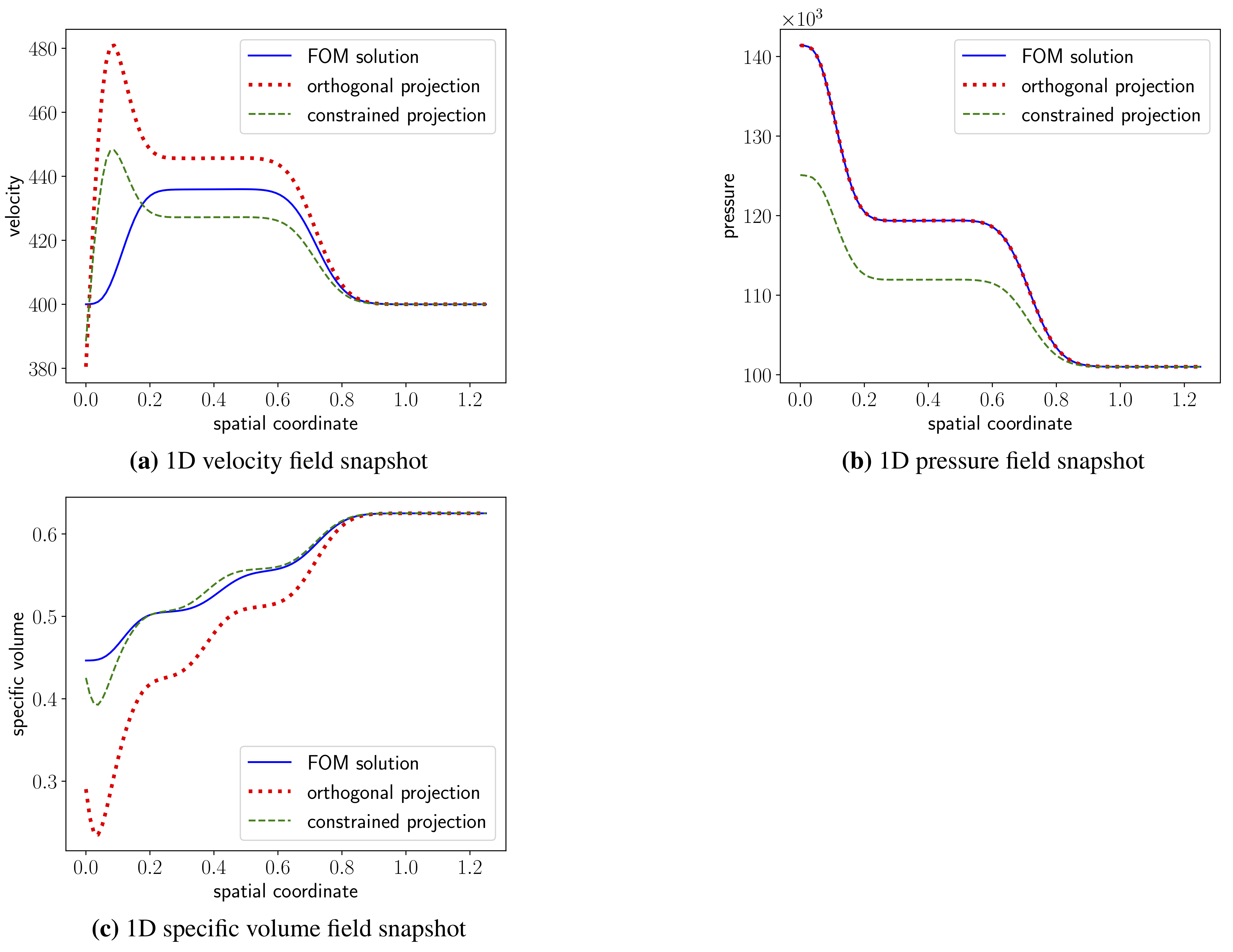
Figure 1 shows a solution snapshot 𝒙n300superscript𝒙𝑛superscript300{\boldsymbol{x}}^{n}\in\mathbb{R}^{300} (blue curve) of the 1D Euler equations (at the parametric configuration 𝝁=(1.6,1.4)𝝁1.61.4{\boldsymbol{\mu}}=(1.6,1.4) and n=200𝑛200n=200, see Section 6.5 for the problem setup), incorporating the velocity field u𝑢u, the pressure field p𝑝p as well as the specific volume field v𝑣v. Additionally, we plot the orthogonal 2superscript2\ell^{2}-projection of this solution onto the affine subspace {𝚽𝒗^+𝒙ref(𝝁)|𝒗^20}conditional-set𝚽^𝒗subscript𝒙ref𝝁^𝒗superscript20\{{\boldsymbol{\Phi}}{\hat{\boldsymbol{v}}}+\boldsymbol{x}_{\mathrm{ref}}({\boldsymbol{\mu}})\,|\,{\hat{\boldsymbol{v}}}\in\mathbb{R}^{20}\} (red curve) using a reduced-order basis 𝚽V20(300)𝚽subscript𝑉20superscript300{\boldsymbol{\Phi}}\in V_{20}(\mathbb{R}^{300}) (which is computed from the first 20 POD modes of the FOM solution at parametric configuration 𝝁=(1.1,1.1)𝝁1.11.1{\boldsymbol{\mu}}=(1.1,1.1) ); the resulting solution 𝒙^n20superscript^𝒙𝑛superscript20{\hat{\boldsymbol{x}}}^{n}\in\mathbb{R}^{20} comprises the solution to the optimization problem

minimize𝝃^20𝚽𝝃^+𝒙ref(𝝁)𝒙n2.\underset{{\hat{\boldsymbol{\xi}}}\in\mathbb{R}^{20}}{\mathrm{minimize\ \ }}\left\lVert{\boldsymbol{\Phi}}{\hat{\boldsymbol{\xi}}}+\boldsymbol{x}_{\mathrm{ref}}{{\boldsymbol{(}}{\boldsymbol{\mu}})}-{\boldsymbol{x}}^{n}\right\rVert_{2}. (79)
Remark 6.1.

The orthogonal-projection optimization problem (79) can be equivalently written as 𝐱^n=𝚽T(𝐱n𝐱ref(𝛍))superscript^𝐱𝑛superscript𝚽𝑇superscript𝐱𝑛subscript𝐱ref𝛍{\hat{\boldsymbol{x}}}^{n}={\boldsymbol{\Phi}}^{T}({\boldsymbol{x}}^{n}-\boldsymbol{x}_{\mathrm{ref}}({\boldsymbol{\mu}})) due to orthogonality of the basis matrix 𝚽𝚽{\boldsymbol{\Phi}}.

Examination of Figure 1 reveals that the absolute values of the pressure field are several orders of magnitude larger than the velocity field, which in turn exhibits values several orders of magnitude larger than the specific-volume field. As a consequence, the orthogonal 2superscript2\ell^{2}-projection yields an approximation that accurately reproduces the pressure field, but effectively neglects the velocity and specific-volume field.

We observe significant over- and undershoots of the orthogonal projection for velocity and specific volume field. To avoid this, we constrain the projection with a field-specific tvb-constraint of shape (57), choosing the upper bound b𝑏b as 150% of the total variation of the FOM snapshot, that is, the tvb-constrained projection reads

minimize𝝃^20𝚽𝝃^+𝒙ref(𝝁)𝒙n2subjecttoc¯L,tvbn,u(𝝃^;𝝁)0c¯L,tvbn,p(𝝃^;𝝁)0c¯L,tvbn,v(𝝃^;𝝁)0,\begin{split}&\underset{{\hat{\boldsymbol{\xi}}}\in\mathbb{R}^{20}}{\mathrm{minimize\ \ }}\left\lVert{\boldsymbol{\Phi}}{\hat{\boldsymbol{\xi}}}+\boldsymbol{x}_{\mathrm{ref}}({\boldsymbol{\mu}})-{\boldsymbol{x}}^{n}\right\rVert_{2}\\ &\mathrm{subject\ to}\quad\bar{c}_{L,\mathrm{tvb}}^{n,u}({\hat{\boldsymbol{\xi}}};{\boldsymbol{\mu}})\geq 0\\ &\hskip 50.0pt\bar{c}_{L,\mathrm{tvb}}^{n,p}({\hat{\boldsymbol{\xi}}};{\boldsymbol{\mu}})\geq 0\\ &\hskip 50.0pt\bar{c}_{L,\mathrm{tvb}}^{n,v}({\hat{\boldsymbol{\xi}}};{\boldsymbol{\mu}})\geq 0,\end{split} (80)

wherein we introduced c¯L,tvbn,u,c¯L,tvbn,psuperscriptsubscript¯𝑐𝐿tvb𝑛𝑢superscriptsubscript¯𝑐𝐿tvb𝑛𝑝\bar{c}_{L,\mathrm{tvb}}^{n,u},\bar{c}_{L,\mathrm{tvb}}^{n,p} and c¯L,tvbn,vsuperscriptsubscript¯𝑐𝐿tvb𝑛𝑣\bar{c}_{L,\mathrm{tvb}}^{n,v} as the tvb-constraint (57) applied to the individual 1D fields u𝑢u, p𝑝p and v𝑣v.

The reconstruction using tvb-constrained projection is depicted in Figure 1 (green curve). Table 1 depicts relative errors as well as violations of the 150% tvb-constraint obtained by the two investigated projections. We observe an improvement in velocity and specific volume field accuracy at an expense of the pressure field reconstruction accuracy, oscillations in velocity and specific volume field could be reduced.

orthogonal projection constrained projection
error velocity pressure specific volume total error velocity pressure specific volume total error
εxnsuperscriptsubscript𝜀x𝑛\varepsilon_{\mathrm{x}}^{n} 4.9% 0.073% 12.4% 0.019% 2.7% 6.1% 2.3% 6.1%
εtvbnsuperscriptsubscript𝜀tvb𝑛\varepsilon_{\mathrm{tvb}}^{n} 73.66 0 0.18 - 0 0 0 -
Table 1: Relative state errors and violation of the tvb-constraint for projection of Euler equations solution snapshot on an affine subspace.
Refer to caption
Figure 1: Exemplary FOM solution snapshot of 1D Euler flow, unconstrained orthogonal projection and tvb-constrained projection on the span of a given reduced-order basis.

6.4 Burgers’ equation

We demonstrate the performance of the proposed formulation on the source-free and inviscid Burgers’ equation

u(z,t;𝝁)t+u(z,t;𝝁)u(z,t;𝝁)z=0,(z,t)[0,L]×[0,T]formulae-sequence𝑢𝑧𝑡𝝁𝑡𝑢𝑧𝑡𝝁𝑢𝑧𝑡𝝁𝑧0for-all𝑧𝑡0𝐿0𝑇\frac{\partial u(z,t;{\boldsymbol{\mu}})}{\partial t}+u(z,t;{\boldsymbol{\mu}})\frac{\partial u(z,t;{\boldsymbol{\mu}})}{\partial z}=0,\quad\forall(z,t)\in[0,L]\times[0,T] (81)

with the parameterized initial condition

u(0,z;𝝁)=ui(z;𝝁)μ2cos(2πμ1100z)+(μ2+1),z(0,L]formulae-sequence𝑢0𝑧𝝁subscript𝑢𝑖𝑧𝝁subscript𝜇22𝜋subscript𝜇1100𝑧subscript𝜇21for-all𝑧0𝐿u(0,z;{\boldsymbol{\mu}})=u_{i}(z;{\boldsymbol{\mu}})\equiv\mu_{2}\cos\left(\frac{2\pi\mu_{1}}{100}z\right)+(\mu_{2}+1),\quad\forall z\in\ (0,L] (82)

and the Dirichlet boundary condition

u(0,t;𝝁)=ui(0;𝝁),t[0,T].formulae-sequence𝑢0𝑡𝝁subscript𝑢𝑖0𝝁for-all𝑡0𝑇u(0,t;{\boldsymbol{\mu}})=u_{i}(0;{\boldsymbol{\mu}}),\quad\forall t\in[0,T]. (83)

Here, u(z,t;𝝁)𝑢𝑧𝑡𝝁u(z,t;{\boldsymbol{\mu}}) denotes the solution of interest, z[0,L]𝑧0𝐿z\in[0,L] denotes the spatial coordinate (with L=100𝐿100L=100 being the right boundary), t[0,T]𝑡0𝑇t\in[0,T] denotes time (with T=30𝑇30T=30 the final time) and 𝝁(μ1,μ2)𝝁subscript𝜇1subscript𝜇2{\boldsymbol{\mu}}\equiv(\mu_{1},\mu_{2}) denote initial-condition parameters corresponding to the frequency and the amplitude (and height), respectively. The parametric domain bounds are given by μ1[0.8;1.2]subscript𝜇10.81.2\mu_{1}\in[0.8;1.2], μ2[0.2;0.6]subscript𝜇20.20.6\mu_{2}\in[0.2;0.6].

6.4.1 Discretization and offline training

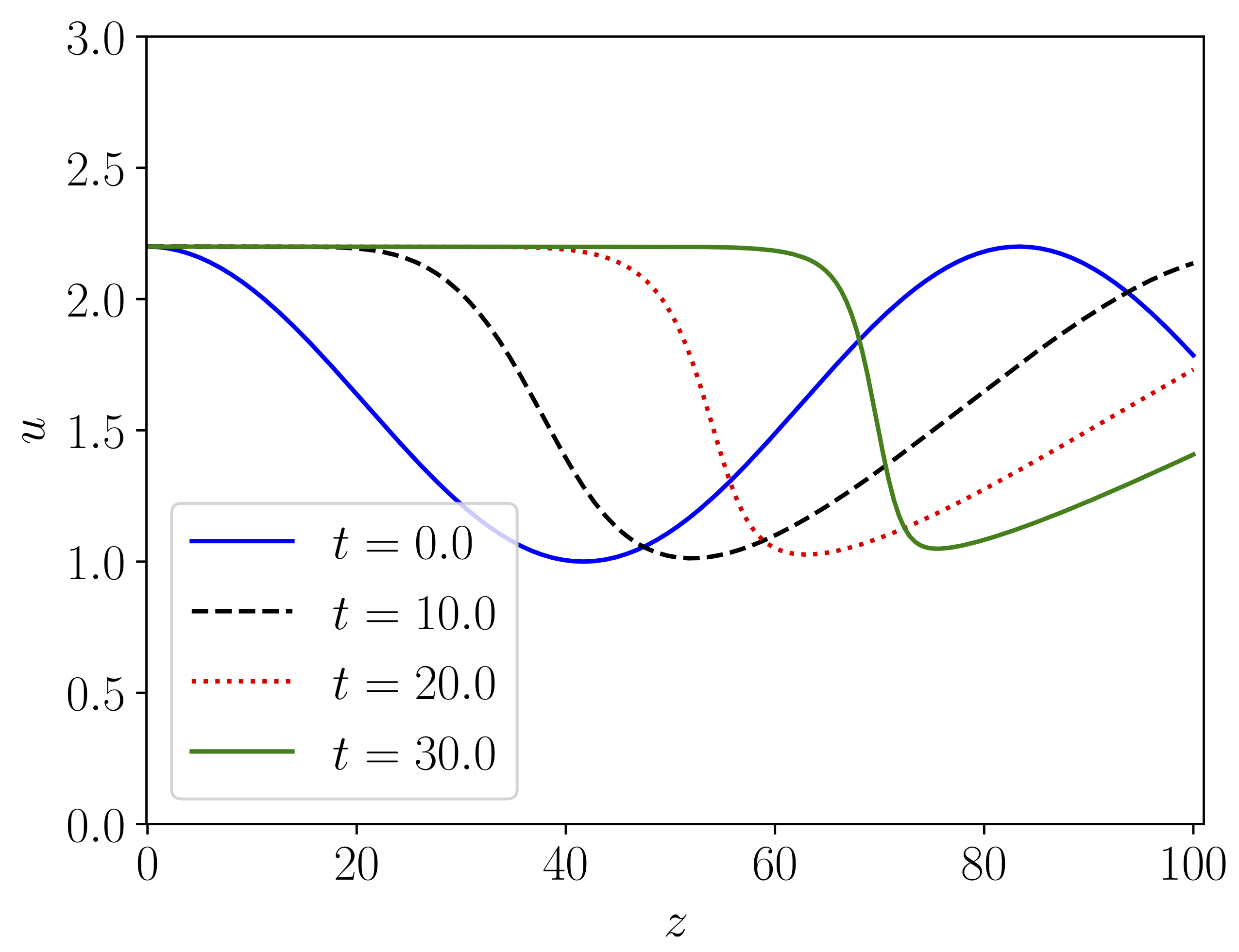
We apply a finite-volume scheme with an upwind flux on a uniformly spaced grid, yielding a model with N=200𝑁200N=200 (i.e., 200 control volumes) degrees of freedom. We apply a backward Euler time discretization with NT=150subscript𝑁𝑇150N_{T}=150 time instances such that Δt=0.2Δ𝑡0.2\Delta t=0.2. Figure 2 depicts the solution at several time steps for a specific parameter instance.
Refer to caption
Figure 2: Numerical solution of Burgers’ equation at different time steps. The depicted solution corresponds to a parametrization of 𝝁=(1.2,0.6)𝝁1.20.6{\boldsymbol{\mu}}=(1.2,0.6).

Training simulations are evaluated on the training set

𝒟train{𝝁traini}i=1ntrain,withntrain=4formulae-sequencesubscript𝒟trainsuperscriptsubscriptsuperscriptsubscript𝝁train𝑖𝑖1subscript𝑛trainwithsubscript𝑛train4\mathcal{D}_{\mathrm{train}}\equiv\{{\boldsymbol{\mu}}_{\mathrm{train}}^{i}\}_{i=1}^{n_{\mathrm{train}}},\quad\mathrm{with}\ n_{\mathrm{train}}=4 (84)

resulting from all combination of μ1{0.8,1.2}subscript𝜇10.81.2\mu_{1}\in\{0.8,1.2\} and μ2{0.2,0.6}subscript𝜇20.20.6\mu_{2}\in\{0.2,0.6\}. The reduced-order basis 𝚽Vp(200)𝚽subscript𝑉𝑝superscript200{\boldsymbol{\Phi}}\in V_{p}(\mathbb{R}^{200}) is computed from the first p𝑝p POD modes of the accumulated snapshot matrix.

6.4.2 Applied constraints

We apply a rsum-constraint of the forms (44) and (46) for constrained Galerkin and LSPG projection, respectively, with a single equality constraint over the sum of all residual entries, that is 𝑪=[1,1,,1]𝑪111{\boldsymbol{C}}=[1,1,\ldots,1] with 𝑪1×200𝑪superscript1200{\boldsymbol{C}}\in\mathbb{R}^{1\times 200}. This constraint can be interpreted as global conservation under certain assumptions, see Ref. [8] for a detailed discussion. Furthermore, given that the Burgers’ equation under consideration is source-free, the numerical solution of the FOM is total variation diminishing, such that we enforce an inequality constraint of the forms (51) and (53) for constrained Galerkin and LSPG projection, respectively.

6.4.3 Results

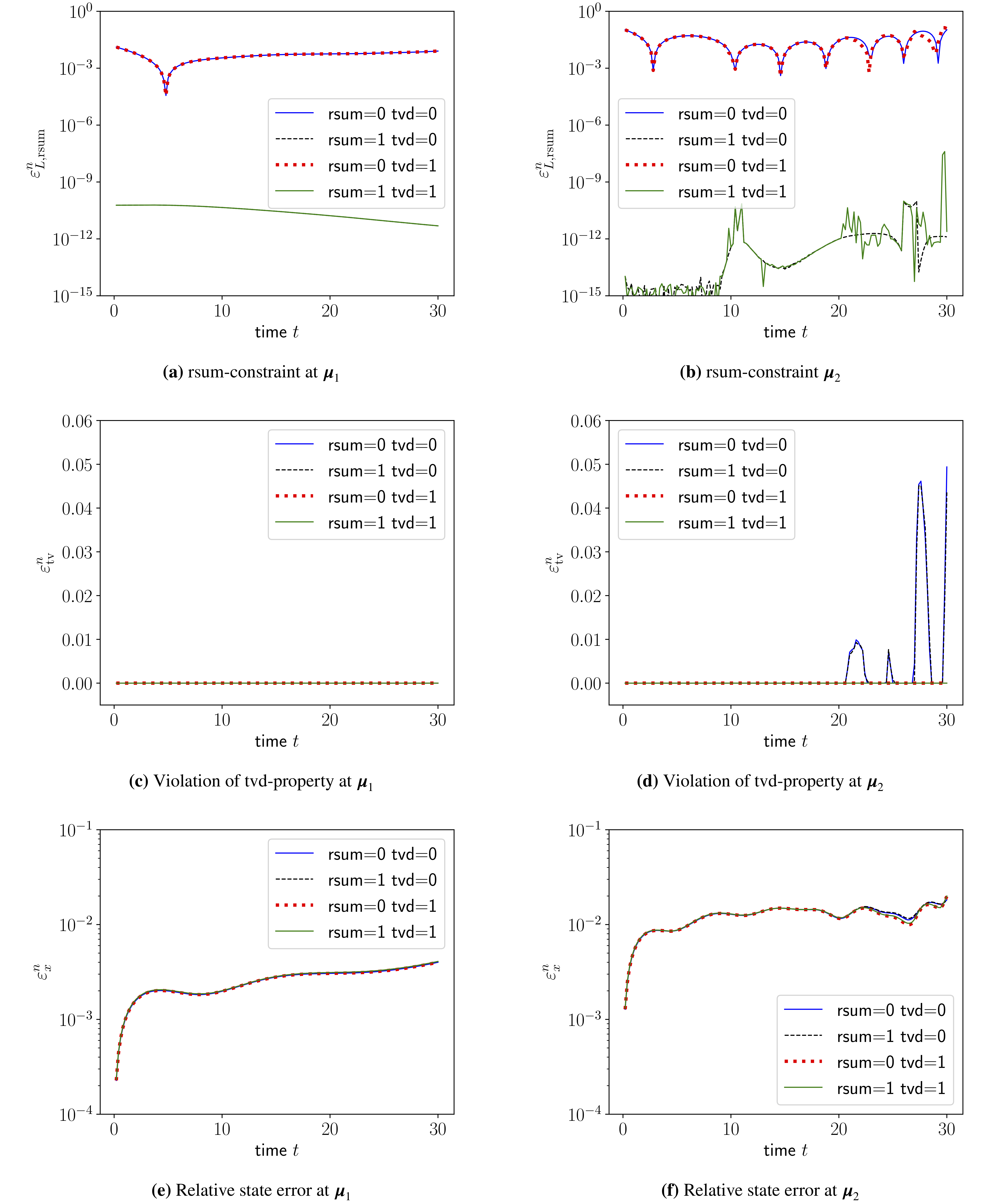
All results reported in this section were produced using the functionality of scipy.optimize.minimize (method=’SLSQP’ with parameters maxiter=100,  ftol=1010superscript101010^{-10}, cf. Section 6.2). Figures 5 and 6 depict error metrics for the Burgers’ flow choosing a reduced dimension of p=10𝑝10p=10. Every model is evaluated at two online parametric configurations, namely 𝝁1=(0.9,0.3)𝒟trainsubscript𝝁10.90.3subscript𝒟train{\boldsymbol{\mu}}_{1}=(0.9,0.3)\not\in\mathcal{D}_{\mathrm{train}} and 𝝁2=(1.3,0.7)𝒟trainsubscript𝝁21.30.7subscript𝒟train{\boldsymbol{\mu}}_{2}=(1.3,0.7)\not\in\mathcal{D}_{\mathrm{train}}. Note that 𝝁1subscript𝝁1{\boldsymbol{\mu}}_{1} and 𝝁2subscript𝝁2{\boldsymbol{\mu}}_{2} correspond to configurations with different complexity in the sense that 𝝁1subscript𝝁1{\boldsymbol{\mu}}_{1} is a setting within the bounds of the training set 𝒟trainsubscript𝒟train\mathcal{D}_{\mathrm{train}} while 𝝁2subscript𝝁2{\boldsymbol{\mu}}_{2} resides outside the training set bounds.

The global rsum-constraint, which can be found in subfigures (a) and (b) indicates that with rsum being in use the corresponding error metrics εG,rsumnsubscriptsuperscript𝜀𝑛𝐺rsum\varepsilon^{n}_{G,\mathrm{rsum}} and εL,rsumnsubscriptsuperscript𝜀𝑛𝐿rsum\varepsilon^{n}_{L,\mathrm{rsum}} decrease locally by several orders of magnitude and achieve near machine precision; this implies that these constraints were feasible.

The violation of the tvd-constraint is depicted in subfigures (c) and (d). Configuration 𝝁1subscript𝝁1{\boldsymbol{\mu}}_{1} fulfills the tvd-constraint for every combination of constraints, even the simple unconstrained ROM is tvd. This changes for configuration 𝝁2subscript𝝁2{\boldsymbol{\mu}}_{2}, for which the unconstrained ROM can not maintain diminishing total variation over the entire time of simulation. Turning the tvd-constraint on yields a regain of the desired property, forcing the ROM to inherit the tvd-property from the FOM. This implies that the tvd-constraint was indeed feasible. Subfigures (e) and (f) indicate that the constraints do not have a negative effect on the state error.

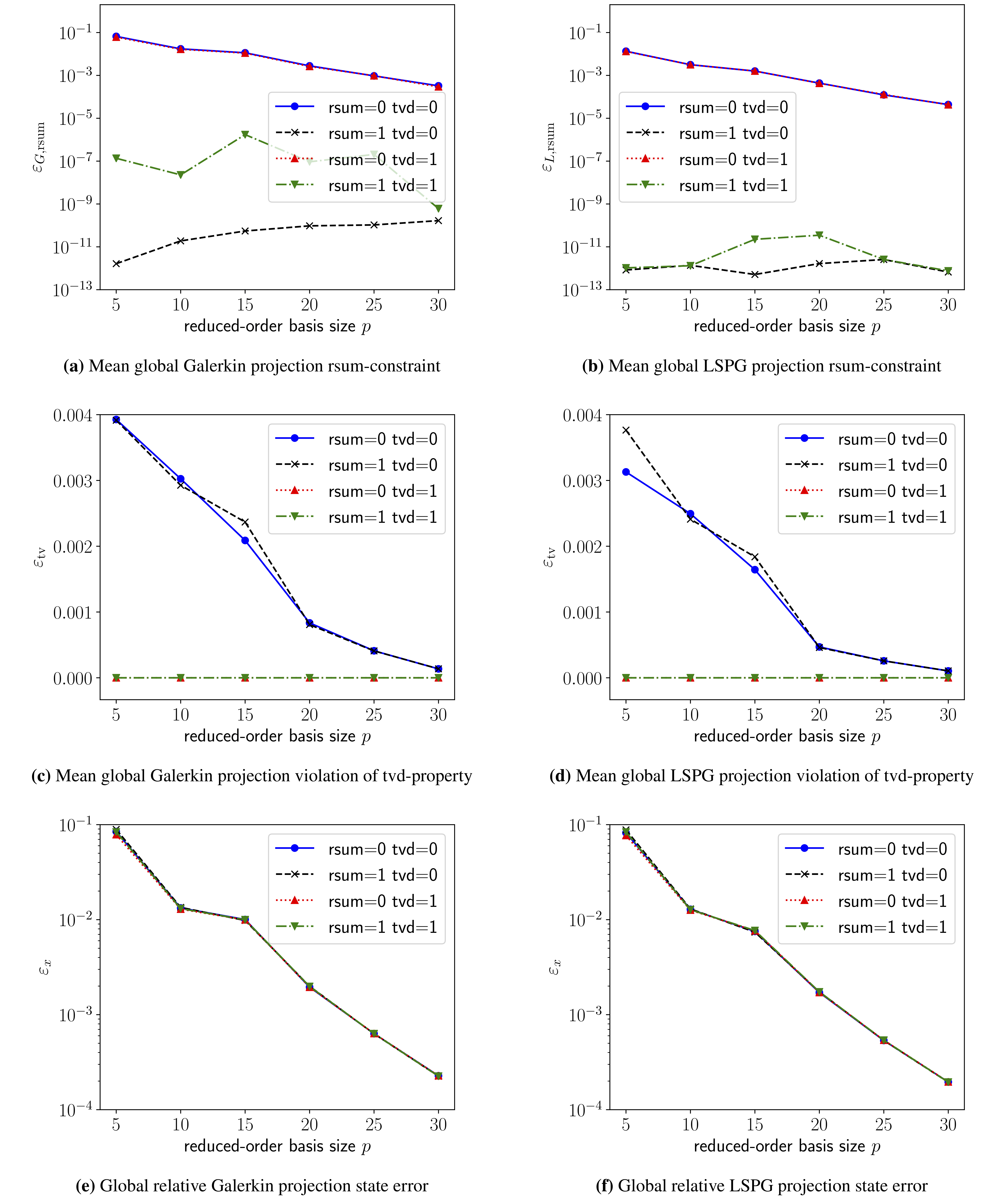
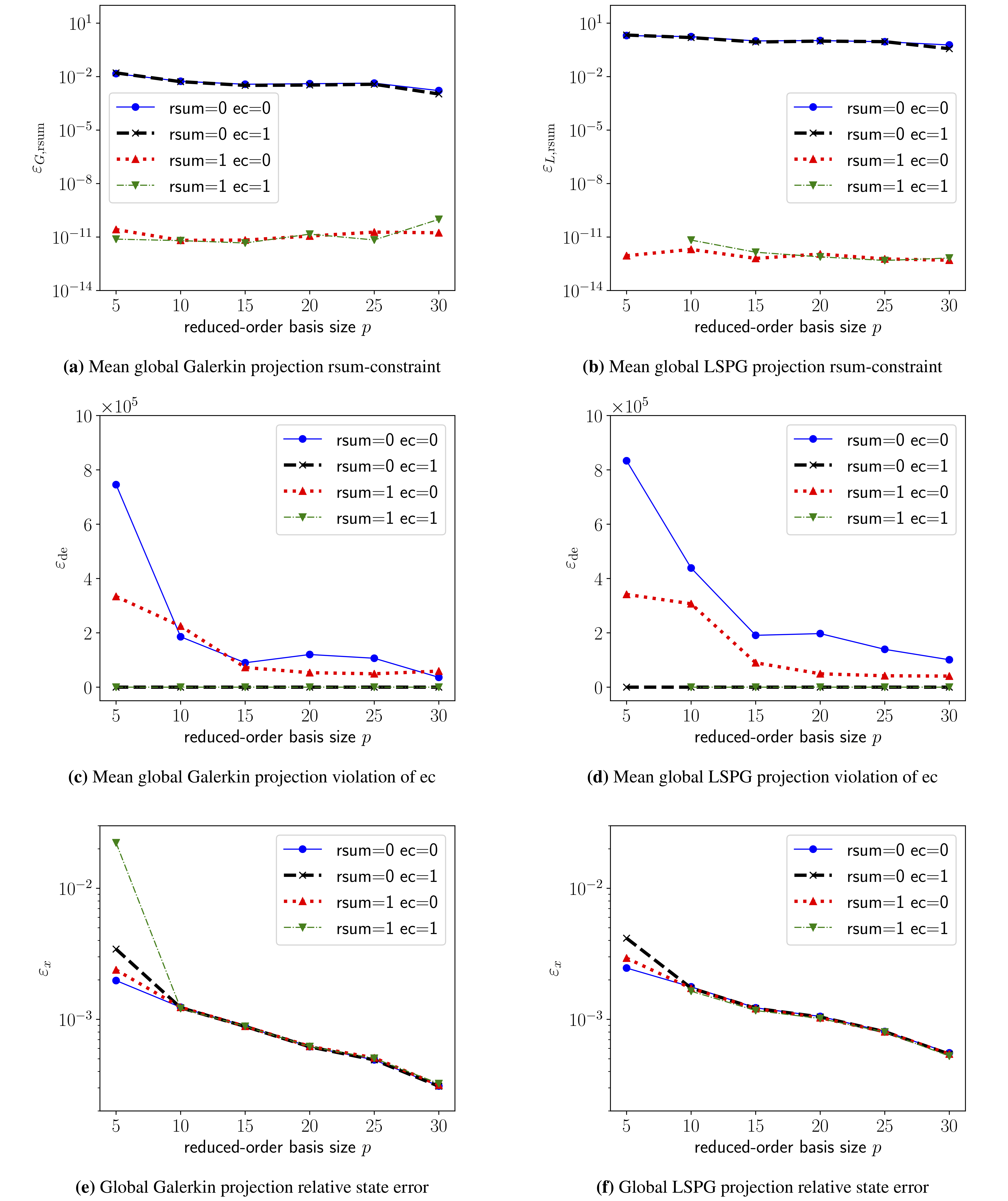
Figure 7 depicts error metrics for 𝝁2subscript𝝁2{\boldsymbol{\mu}}_{2} over a variable reduced-order basis size p𝑝p. A refinement in p𝑝p results in decreasing error metrics for the unconstrained models. However, the rsum- as well as the tvd-constraint yield better accuracy in the corresponding error metrics over the entire range, especially for small basis dimensions.

6.5 Euler equations

We now present an ideal gas flow described by the 1D Euler equations

u(z,t;𝝁)t+u(z,t;𝝁)u(z,t;𝝁)z+v(z,t;𝝁)p(z,t;𝝁)z𝑢𝑧𝑡𝝁𝑡𝑢𝑧𝑡𝝁𝑢𝑧𝑡𝝁𝑧𝑣𝑧𝑡𝝁𝑝𝑧𝑡𝝁𝑧\displaystyle\frac{\partial u(z,t;{\boldsymbol{\mu}})}{\partial t}+u(z,t;{\boldsymbol{\mu}})\frac{\partial u(z,t;{\boldsymbol{\mu}})}{\partial z}+v(z,t;{\boldsymbol{\mu}})\frac{\partial p(z,t;{\boldsymbol{\mu}})}{\partial z} =0,(z,t)[0,L]×[0,T],formulae-sequenceabsent0for-all𝑧𝑡0𝐿0𝑇\displaystyle=0,\quad\forall(z,t)\in[0,L]\times[0,T], (85)
p(z,t;𝝁)t+u(z,t;𝝁)p(z,t;𝝁)z+γp(z,t;𝝁)u(z,t;𝝁)z𝑝𝑧𝑡𝝁𝑡𝑢𝑧𝑡𝝁𝑝𝑧𝑡𝝁𝑧𝛾𝑝𝑧𝑡𝝁𝑢𝑧𝑡𝝁𝑧\displaystyle\frac{\partial p(z,t;{\boldsymbol{\mu}})}{\partial t}+u(z,t;{\boldsymbol{\mu}})\frac{\partial p(z,t;{\boldsymbol{\mu}})}{\partial z}+\gamma p(z,t;{\boldsymbol{\mu}})\frac{\partial u(z,t;{\boldsymbol{\mu}})}{\partial z} =0,(z,t)[0,L]×[0,T],formulae-sequenceabsent0for-all𝑧𝑡0𝐿0𝑇\displaystyle=0,\quad\forall(z,t)\in[0,L]\times[0,T], (86)
v(z,t;𝝁)t+u(z,t;𝝁)v(z,t;𝝁)zv(z,t;𝝁)u(z,t;𝝁)z𝑣𝑧𝑡𝝁𝑡𝑢𝑧𝑡𝝁𝑣𝑧𝑡𝝁𝑧𝑣𝑧𝑡𝝁𝑢𝑧𝑡𝝁𝑧\displaystyle\frac{\partial v(z,t;{\boldsymbol{\mu}})}{\partial t}+u(z,t;{\boldsymbol{\mu}})\frac{\partial v(z,t;{\boldsymbol{\mu}})}{\partial z}-v(z,t;{\boldsymbol{\mu}})\frac{\partial u(z,t;{\boldsymbol{\mu}})}{\partial z} =0,(z,t)[0,L]×[0,T],formulae-sequenceabsent0for-all𝑧𝑡0𝐿0𝑇\displaystyle=0,\quad\forall(z,t)\in[0,L]\times[0,T], (87)

where the solution is composed of the velocity field u(z,t;𝝁)𝑢𝑧𝑡𝝁u(z,t;{\boldsymbol{\mu}}), the pressure field p(z,t;𝝁)𝑝𝑧𝑡𝝁p(z,t;{\boldsymbol{\mu}}), and the mass-specific volume field v(z,t;𝝁)𝑣𝑧𝑡𝝁v(z,t;{\boldsymbol{\mu}}); here, γ𝛾\gamma denotes the isentropic exponent. Parametrization in terms of the 2D parameter vector 𝝁(μ1,μ2)𝝁subscript𝜇1subscript𝜇2{\boldsymbol{\mu}}\equiv(\mu_{1},\mu_{2}) is introduced within the initial condition as well as the boundary condition. The initial condition reads

u(z,0;𝝁)=u0,p(z,0;𝝁)=p0,v(z,0;𝝁)=1μ1,z(0,L],formulae-sequence𝑢𝑧0𝝁subscript𝑢0formulae-sequence𝑝𝑧0𝝁subscript𝑝0formulae-sequence𝑣𝑧0𝝁1subscript𝜇1for-all𝑧0𝐿\displaystyle u(z,0;{\boldsymbol{\mu}})=u_{0},\quad p(z,0;{\boldsymbol{\mu}})=p_{0},\quad v(z,0;{\boldsymbol{\mu}})=\frac{1}{\mu_{1}},\quad\forall z\in(0,L], (88)

and we denote the boundary condition by

u(0,t;𝝁)=udbc=u0,p(0,t;𝝁)=pdbc=p0μ2,v(0,t;𝝁)=vdbc=1μ1μ2,t[0,T].formulae-sequence𝑢0𝑡𝝁subscript𝑢dbcsubscript𝑢0𝑝0𝑡𝝁subscript𝑝dbcsubscript𝑝0subscript𝜇2𝑣0𝑡𝝁subscript𝑣dbc1subscript𝜇1subscript𝜇2for-all𝑡0𝑇\displaystyle u(0,t;{\boldsymbol{\mu}})=u_{\mathrm{dbc}}=u_{0},\quad p(0,t;{\boldsymbol{\mu}})=p_{\mathrm{dbc}}=p_{0}\mu_{2},\quad v(0,t;{\boldsymbol{\mu}})=v_{\mathrm{dbc}}=\frac{1}{\mu_{1}\mu_{2}},\quad\forall t\in[0,T]. (89)

The parametrization can be physically interpreted as

μ1subscript𝜇1\displaystyle\mu_{1} =ρ0,μ2=pdbcp0=ρdbcρ0.formulae-sequenceabsentsubscript𝜌0subscript𝜇2subscript𝑝dbcsubscript𝑝0subscript𝜌dbcsubscript𝜌0\displaystyle=\rho_{0},\qquad\mu_{2}=\frac{p_{\mathrm{dbc}}}{p_{0}}=\frac{\rho_{\mathrm{dbc}}}{\rho_{0}}. (90)

That is, μ1subscript𝜇1\mu_{1} corresponds to the initial density of the fluid, while μ2subscript𝜇2\mu_{2} corresponds to the ratio of the pressure boundary condition and the initial pressure value and at the same time the ratio of the density boundary condition and the initial density. Consequently, the described setup can be interpreted as a 1D model of a tube, which is continuously traversed by an ideal gas, while at a specific instance in time (t=0𝑡0t=0), a sudden change in the fluid properties appears at the inlet of the tube.

The constants introduced are set to γ=1.4𝛾1.4\gamma=1.4, u0=400mssubscript𝑢0400m𝑠u_{0}=400\frac{\mathrm{m}}{s}, p0=101000Pasubscript𝑝0101000Pap_{0}=101000\mathrm{Pa}, L=1.25m𝐿1.25mL=1.25\mathrm{m} and T=0.001s𝑇0.001sT=0.001\mathrm{s}, and the parametric domain bounds are given by μ1[1.1kgm3;1.6kgm3]subscript𝜇11.1kgsuperscriptm31.6kgsuperscriptm3\mu_{1}\in[1.1\frac{\mathrm{kg}}{\mathrm{m}^{3}};1.6\frac{\mathrm{kg}}{\mathrm{m}^{3}}], μ2[1.1;1.4]subscript𝜇21.11.4\mu_{2}\in[1.1;1.4]. Given that the speed of sound is c=p0ρ0γ<u0𝑐subscript𝑝0subscript𝜌0𝛾subscript𝑢0c=\sqrt{\frac{p_{0}}{\rho_{0}}\gamma}<u_{0} (recall that ρ0=μ1subscript𝜌0subscript𝜇1\rho_{0}=\mu_{1}), the flow under consideration is classified as supersonic.
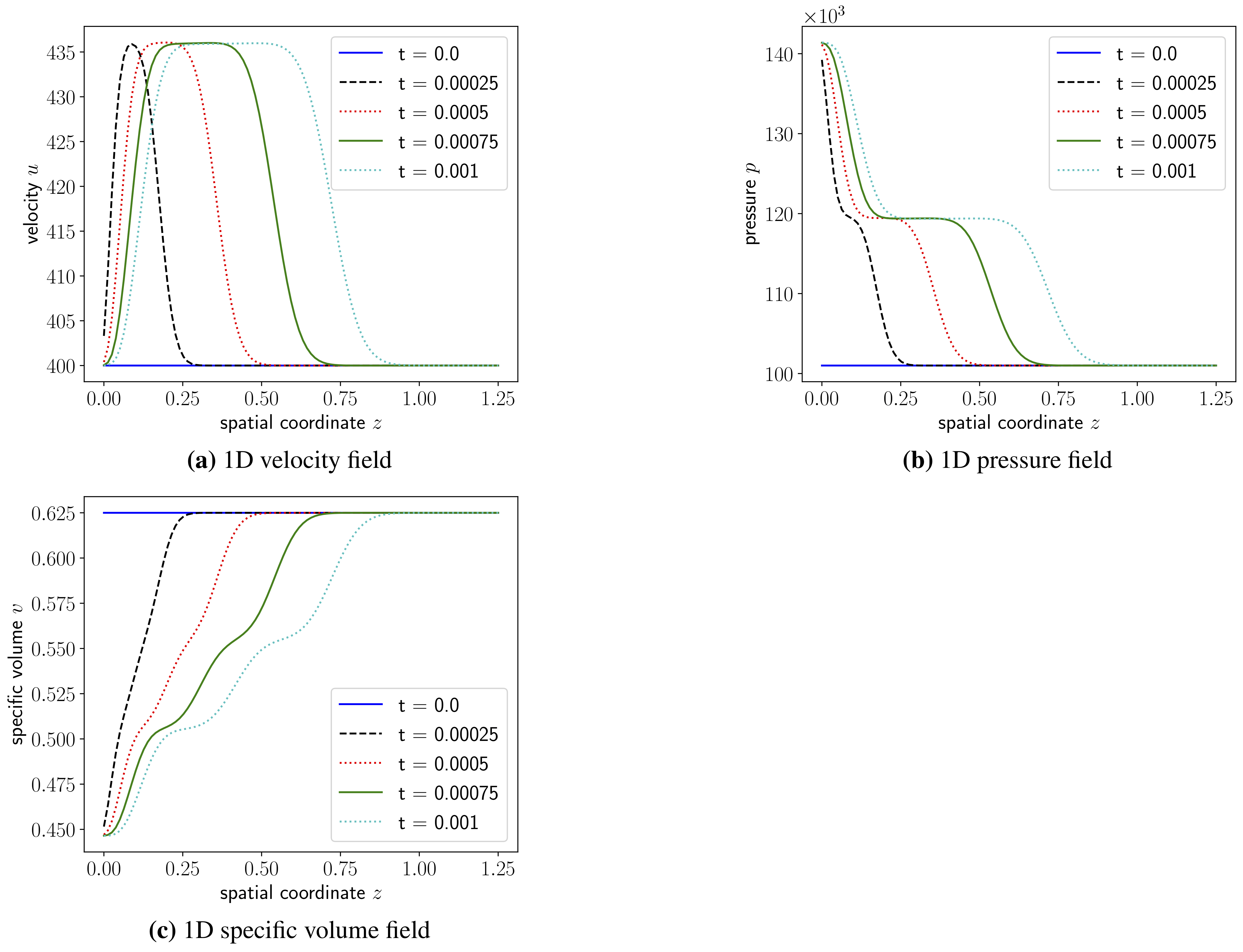
Refer to caption
Figure 3: Numerical solution of Euler equations at different time steps. The depicted solution corresponds to a parametrization of 𝝁=(1.6,1.4)𝝁1.61.4{\boldsymbol{\mu}}=(1.6,1.4).

6.5.1 Discretization and offline training

We apply a finite-difference spatial discretization scheme on a uniform grid with backward finite differences and N=300𝑁300N=300 (i.e., 100 degrees of freedom for u,p,v𝑢𝑝𝑣u,p,v each) and NTsubscript𝑁𝑇N_{T} time steps (NT=200subscript𝑁𝑇200N_{T}=200 and NT=600subscript𝑁𝑇600N_{T}=600 will be considered further down below). Time stepping is performed with the explicit Euler method, see Figure 3 for an exemplary solution at several time steps for a specific parameter instance.

Training simulations are evaluated on the training set

𝒟train{𝝁traini}i=1ntrain,withntrain=4formulae-sequencesubscript𝒟trainsuperscriptsubscriptsuperscriptsubscript𝝁train𝑖𝑖1subscript𝑛trainwithsubscript𝑛train4\mathcal{D}_{\mathrm{train}}\equiv\{{\boldsymbol{\mu}}_{\mathrm{train}}^{i}\}_{i=1}^{n_{\mathrm{train}}},\quad\mathrm{with}\ n_{\mathrm{train}}=4 (91)

resulting from all combination of μ1{1.1,1.6}subscript𝜇11.11.6\mu_{1}\in\{1.1,1.6\} and μ2{1.1,1.4}subscript𝜇21.11.4\mu_{2}\in\{1.1,1.4\}. A reduced-order basis 𝚽Vp(300)𝚽subscript𝑉𝑝superscript300{\boldsymbol{\Phi}}\in V_{p}(\mathbb{R}^{300}) is computed from the first p𝑝p POD modes of the training simulation snapshots.

Remark 6.2.

Unconstrained Galerkin and LSPG projection ROMs are equivalent for time discretization by an explicit linear multistep scheme, see Ref. [7]. As a consequence, we depict only one curve for both unconstrained projections in B.

6.5.2 Applied constraints

We apply a quantity-specific tvb-constraint of the forms (56) and (57). By quantity-specific we mean that total variation is bounded for each quantity (u𝑢u, p𝑝p and v𝑣v) independently, which results in three inequality constraints. Three total variation bounds (one for each quantity) are computed as 120 % of the quantity-specific maximum total variation values of all training simulation snapshots.

Remark 6.3.

Estimating a total variation bound from training simulation snapshots can be seen as a consistent extension of the snapshot collection method for the construction of a low-dimensional solution subspace, which corresponds to kinematically constraining the space of all admissible solution states. In this context, a total variation bound computed from solution snapshots simply corresponds to further kinematically constraining the state.

6.5.3 Results

All results reported in this section were produced using the functionality of scipy.optimize.minimize (method=’trust-constr’ with parameters maxiter=250, gtol=106superscript10610^{-6}, xtol=106superscript10610^{-6}, barrier_tol=106superscript10610^{-6} for Galerkin projection and method=’SLSQP’ with parameters maxiter=250, ftol=106superscript10610^{-6} for LSPG projection, cf. Section 6.2). Figures 8 and 9 depict results collected from constrained and unconstrained Galerkin and LSPG projections choosing a reduced dimension of p=20𝑝20p=20. Plots in the left column are computed from 200 time steps, while plots in the right column are computed from a finer discretization in time using 600 time steps. Figure 8 illustrates relative state errors (67) for the three quantities (velocity εx,unsubscriptsuperscript𝜀𝑛𝑥𝑢\varepsilon^{n}_{x,u}, pressure εx,pnsubscriptsuperscript𝜀𝑛𝑥𝑝\varepsilon^{n}_{x,p}, specific volume εx,vnsubscriptsuperscript𝜀𝑛𝑥𝑣\varepsilon^{n}_{x,v}) involved in the solution of the Euler equations. The presence of the tvb-constraint improves the state errors. On closer inspection, the plots show an overlap of constrained and unconstrained curves up to a certain point in time, at which the curves split. This observation can be explained by inspecting Figure 9, which depicts quantity-specific total variations as well as the applied total variation bound. As a result, the curves in Figure 8 overlap until the tvb-constraint is active. When the unconstrained curve crosses the total variation bound, state errors start to separate.

Also the total variations in Figure 9 overlap initially and split, when the tvb-constraint becomes active. However, tvb-constrained curves (especially pronounced for velocity and pressure) still run above the total variation bound for the Galerkin projection, such that the tvb-constraint (55) is not fulfilled. We reference Remark 4.2 for the explanation of this behavior, highlighting that the constraint violation at hand is a consequence of time discretization. Using a finer discretization in time (600 instead of 200 time steps) results in lower constraint violation for the Galerkin projection, which can be seen from right column plots of Figure 9. For the LSPG projection, the applied total variation bound is strictly respected for 200 as well as 600 time steps.

Figure 10 depicts mean global error metrics. Discussing the unconstrained ROM first, we observe an initial increase of the state error for all quantities with a peak at p=20𝑝20p=20, followed by a sudden decrease with increasing reduced-order basis size until p=30𝑝30p=30. The tvb-constraint violation plots explain the peak at p=20𝑝20p=20, showing that the unconstrained ROM solution becomes oscillatory. A further increase in p𝑝p until p=30𝑝30p=30 leads to a rather accurate ROM, which reflects in the state space error as well as the tvb-constraint violation plots. For further increase in p𝑝p, the unconstrained ROM again becomes oscillatory at p=35𝑝35p=35 and eventually unstable at p=40𝑝40p=40.

In contrast, both tvb-constrained Galerkin and LSPG projection ROMs show only slight (Galerkin projection) or no (LSPG projection) violation of the tvb-constraint over all evaluated reduced-order basis sizes and also achieve a stable solution, when the unconstrained ROM becomes unstable (p=40𝑝40p=40).

We observe that state errors for some p𝑝p-values are slightly worse with tvb-constraint activated, while the tvb-constraint is almost fulfilled by the unconstrained curve (p=25𝑝25p=25 and p=30𝑝30p=30). The conclusion from the current example is that the tvb-constraint is helpful when the unconstrained ROM severely violates that property, while it can become harmful (for the state error) when the unconstrained ROM is sufficiently accurate by itself.

6.6 Diffusion equation

We solve a nonlinear, non-homogeneous diffusion equation of the shape

ρcθ(t,y,z;𝝁)t(λ(θ)θ(t,y,z;𝝁))=s(t,y,z;𝝁),(t,y,z)[0,T]×[0,L]×[0,L]formulae-sequence𝜌𝑐𝜃𝑡𝑦𝑧𝝁𝑡𝜆𝜃𝜃𝑡𝑦𝑧𝝁𝑠𝑡𝑦𝑧𝝁for-all𝑡𝑦𝑧0𝑇0𝐿0𝐿\rho c\frac{\partial\theta(t,y,z;{\boldsymbol{\mu}})}{\partial t}-\nabla\cdot(\lambda(\theta)\nabla\theta(t,y,z;{\boldsymbol{\mu}}))=s(t,y,z;{\boldsymbol{\mu}}),\quad\forall(t,y,z)\in[0,T]\times[0,L]\times[0,L] (92)

with the initial condition

θ(0,y,z;𝝁)=300,(y,z)[0,L]×[0,L],formulae-sequence𝜃0𝑦𝑧𝝁300for-all𝑦𝑧0𝐿0𝐿\theta(0,y,z;{\boldsymbol{\mu}})=300,\quad\forall(y,z)\in[0,L]\times[0,L], (93)

adiabatic boundary conditions

θ(t,y,z;𝝁)𝒏=0,(t,z,y)[0,T]×{0,L}×{0,L},formulae-sequence𝜃𝑡𝑦𝑧𝝁𝒏0for-all𝑡𝑧𝑦0𝑇0𝐿0𝐿\nabla\theta(t,y,z;{\boldsymbol{\mu}})\cdot{\boldsymbol{n}}=0,\quad\forall(t,z,y)\in[0,T]\times\{0,L\}\times\{0,L\}, (94)

a parameterized source

s(t,y,z;𝝁)=μ1δ(y(0.5+μ4sin(2πμ3t))δ(z0.2)s1+μ2δ(y(0.5μ4sin(2πμ3t))δ(z0.5)s2,s(t,y,z;{\boldsymbol{\mu}})=\underbrace{\mu_{1}\delta(y-(0.5+\mu_{4}\sin(2\pi\mu_{3}t))\delta(z-0.2)}_{s_{1}}+\underbrace{\mu_{2}\delta(y-(0.5-\mu_{4}\sin(2\pi\mu_{3}t))\delta(z-0.5)}_{s_{2}}, (95)

and a temperature dependent heat conductivity given by

λ(θ)=(θ300)+50.𝜆𝜃𝜃30050\lambda(\theta)=(\theta-300)+50. (96)

Therein we introduced the area density ρ=8000kg/m2𝜌8000kgsuperscriptm2\rho=8000\ \mathrm{kg}/\mathrm{m}^{2}, mass-specific heat capacity c=500J/(kgK)𝑐500JkgKc=500\ \mathrm{J}/(\mathrm{kg\ K}), temperature θ[K]𝜃delimited-[]K\theta\ [\mathrm{K}], thermal conductivity λ[W/(mK)]𝜆delimited-[]WmK\lambda[\mathrm{W}/(\mathrm{m\ K})], the time t[0,T]𝑡0𝑇t\in[0,T] (with T=10000s𝑇10000sT=10000\ \mathrm{s} being the end time) and spatial coordinates (y,z)[0,L]×[0,L]𝑦𝑧0𝐿0𝐿(y,z)\in[0,L]\times[0,L] (with L=1m𝐿1mL=1\ \mathrm{m} describing the domain size). The parameterized source s𝑠s consists of two dirac delta δ𝛿\delta pulses s1subscript𝑠1s_{1} and s2subscript𝑠2s_{2}, which are moving in y𝑦y-direction in time. Thereby μ1[W/m2]subscript𝜇1delimited-[]Wsuperscriptm2\mu_{1}\ [\mathrm{W}/\mathrm{m}^{2}] and μ2[W/m2]subscript𝜇2delimited-[]Wsuperscriptm2\mu_{2}\ [\mathrm{W}/\mathrm{m}^{2}] are the source strengths, μ3[1/s]subscript𝜇3delimited-[]1s\mu_{3}\ [1/\mathrm{s}] is the moving frequency and μ4[m]subscript𝜇4delimited-[]m\mu_{4}\ [\mathrm{m}] the amplitude.

6.6.1 Discretization and offline training

We apply a central finite difference scheme for spatial discretization on a uniform grid yielding N=1089𝑁1089N=1089 degrees of freedom (33 in each coordinate axis), and employ the implicit Euler time discretization method with NT=100subscript𝑁𝑇100N_{T}=100 time steps. Figure 4 depicts an exemplary solution at parameter instance 𝝁=(106,106,104,0.2)𝝁superscript106superscript106superscript1040.2{\boldsymbol{\mu}}=(-10^{6},10^{6},10^{-4},0.2) including a source and a sink (negative source strength).

Training simulations are evaluated on the training set

𝒟train{𝝁traini}i=1ntrain,withntrain=8formulae-sequencesubscript𝒟trainsuperscriptsubscriptsuperscriptsubscript𝝁train𝑖𝑖1subscript𝑛trainwithsubscript𝑛train8\mathcal{D}_{\mathrm{train}}\equiv\{{\boldsymbol{\mu}}_{\mathrm{train}}^{i}\}_{i=1}^{n_{\mathrm{train}}},\quad\mathrm{with}\ n_{\mathrm{train}}=8 (97)

resulting from all combinations of (μ1,μ2){(1.1×106,0.9×106),(106,106)},μ3{5×105,15×105},μ4{0.1,0.3}formulae-sequencesubscript𝜇1subscript𝜇21.1superscript1060.9superscript106superscript106superscript106formulae-sequencesubscript𝜇35superscript10515superscript105subscript𝜇40.10.3(\mu_{1},\mu_{2})\in\{(-1.1\times 10^{6},0.9\times 10^{-6}),(-10^{6},10^{-6})\},\mu_{3}\in\{5\times 10^{-5},15\times 10^{-5}\},\mu_{4}\in\{0.1,0.3\} and the reduced-order basis 𝚽Vp(1089)𝚽subscript𝑉𝑝superscript1089{\boldsymbol{\Phi}}\in V_{p}(\mathbb{R}^{1089}) is computed from the first p𝑝p POD modes of the accumulated snapshot matrix.
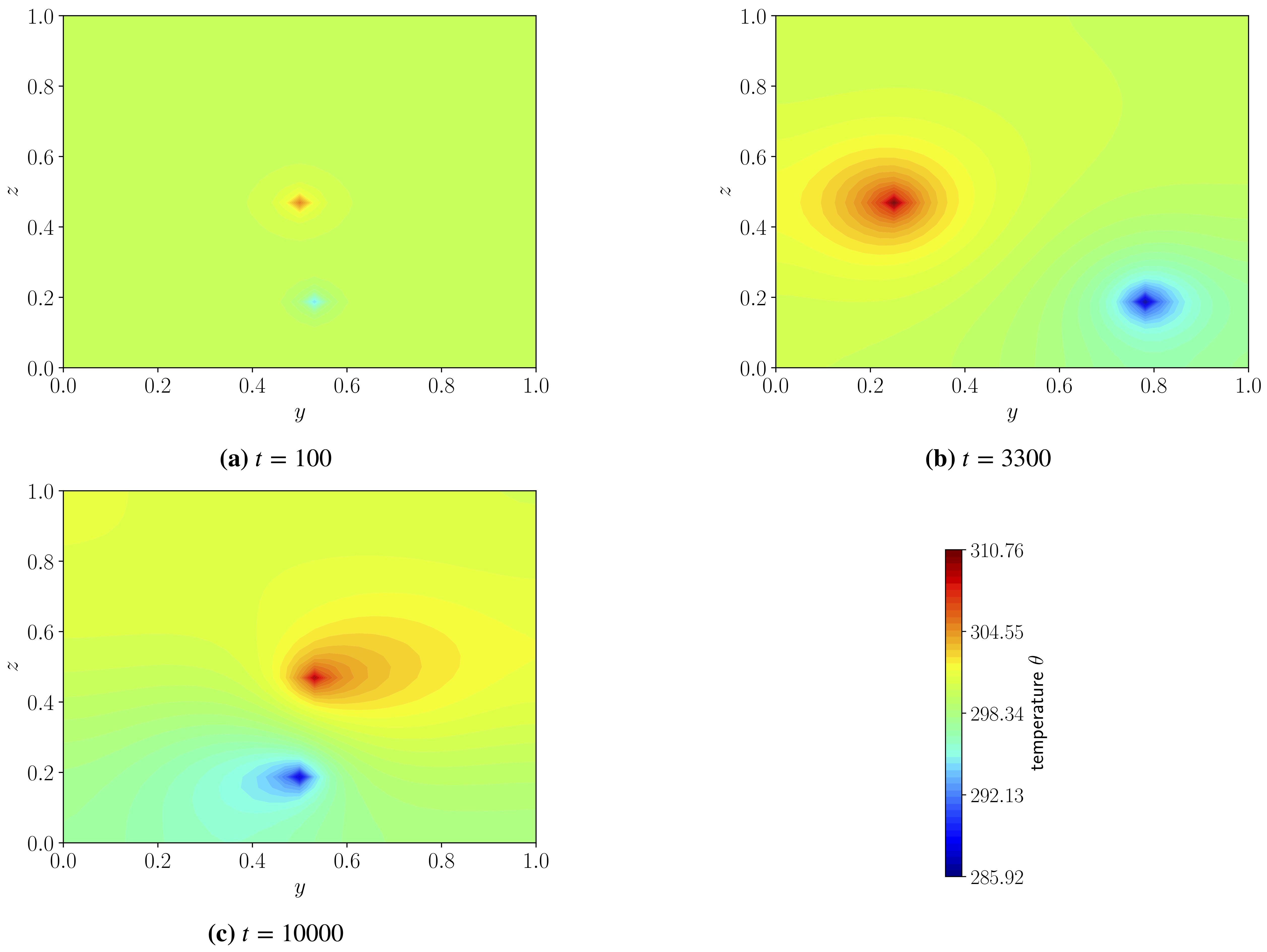
Refer to caption
Figure 4: Numerical solution of nonlinear diffusion equation at different time steps. The depicted solution corresponds to a parametrization of 𝝁=(106,106,104,0.2)𝝁superscript106superscript106superscript1040.2{\boldsymbol{\mu}}=(-10^{6},10^{6},10^{-4},0.2).

6.6.2 Applied constraints

We investigate the performance of the proposed reduced-order models for the exemplary parametrization

𝝁=(106,106,104,0.2)𝝁superscript106superscript106superscript1040.2{\boldsymbol{\mu}}=(-10^{6},10^{6},10^{-4},0.2) (98)

applying a rsum-constraint of the forms (44) and (46) and an ec-constraint of the forms (63) and (65). The rsum-constraint is set to two equality constraints overlapping in 100 elements, that is

𝑪=[100111110000 1]2×1089.𝑪delimited-[]100subscript1111100001superscript21089{\boldsymbol{C}}=\left[\begin{array}[]{l}1\ \ \ldots\\ 0\ldots 0\end{array}\right.\underbrace{\begin{array}[]{l}1\ldots 1\\ 1\ldots 1\end{array}}_{100}\left.\begin{array}[]{l}0\ldots 0\\ \ldots\ \ 1\end{array}\right]\in\mathbb{R}^{2\times 1089}. (99)

The ec-constraint resolves to a simple form in case of the investigated computational example. The global energy of the computational domain in the continuous setting results from

e=0101ρcθ(t,y,z;𝝁)𝑑y𝑑z=ρc0101θ(t,y,z;𝝁)𝑑y𝑑z.𝑒superscriptsubscript01superscriptsubscript01𝜌𝑐𝜃𝑡𝑦𝑧𝝁differential-d𝑦differential-d𝑧𝜌𝑐superscriptsubscript01superscriptsubscript01𝜃𝑡𝑦𝑧𝝁differential-d𝑦differential-d𝑧e=\int_{0}^{1}\int_{0}^{1}\rho c\theta(t,y,z;{\boldsymbol{\mu}})\ dydz=\rho c\int_{0}^{1}\int_{0}^{1}\theta(t,y,z;{\boldsymbol{\mu}})\ dydz. (100)

Assuming 𝒙(t;𝝁)𝒙𝑡𝝁{\boldsymbol{x}}(t;{\boldsymbol{\mu}}) to be a numerical approximation of the (spatially uniform) discretized temperature field θ(t,y,z;𝝁)𝜃𝑡𝑦𝑧𝝁\theta(t,y,z;{\boldsymbol{\mu}}), global energy (100) can be expressed as

e=E(𝒙)=αρc𝟏T𝒙,𝑒𝐸𝒙𝛼𝜌𝑐superscript1𝑇𝒙e=E({\boldsymbol{x}})=\alpha\rho c{\boldsymbol{1}}^{T}{\boldsymbol{x}}, (101)

wherein α𝛼\alpha is a proportionality constant depending on the spatial discretization (in our case α=1Nm2=11089m2𝛼1𝑁superscriptm211089superscriptm2\alpha=\frac{1}{N}\mathrm{m}^{2}=\frac{1}{1089}\mathrm{m}^{2}) and 𝟏1{\boldsymbol{1}} is a vector of ones. Additionally, source and sink in (98) are of the same absolute strength, which (recalling the adiabatic boundary condition (94)) results in a vanishing energy intake S(t;𝝁)𝑆𝑡𝝁S(t;{\boldsymbol{\mu}}) such that energy conservation (62) can be expressed as

αρc𝟏T𝒙˙=0𝛼𝜌𝑐superscript1𝑇˙𝒙0\alpha\rho c{\boldsymbol{1}}^{T}{\dot{\boldsymbol{x}}}=0 (102)

or simply

𝟏T𝒙˙=0.superscript1𝑇˙𝒙0{\boldsymbol{1}}^{T}{\dot{\boldsymbol{x}}}=0. (103)

6.6.3 Results

All results reported in this section were produced using the functionality of scipy.optimize.minimize (method=’SLSQP’ with parameters maxiter=100, ftol=1010superscript101010^{-10}, cf. Section 6.2). Figure 11 depicts the violation of the rsum-constraint (68), (69), the deviation of system energy from its initial state (72) and the relative state error (67) for both Galerkin projection and LSPG projection at the parametric configuration (98) and a reduced dimension of p=10𝑝10p=10. Note that in case of the present example, energy conservation corresponds to a constant system energy, such that energy deviation from the initial state can be interpreted as a violation of conservation of energy. As a result, the rsum-constraint decreases the corresponding error metric by several orders of magnitude to nearly zero, implying feasibility of the rsum-constraint. Similarly, the error in energy conservation drops to nearly zero whenever the ec-constraint is activated, also implying feasibility of this constraint. However, both of these constraints have negligible effect on the state error in this particular case.

Figure 12 reports global error metrics as a function of ROM dimension p𝑝p. In all cases, the state error decreases monotonically with increased basis dimension. For any reduced dimension, enforcing the appropriate constraint has a more substantial effect on satisfying the rsum-constraint and ec-constraint than simply increasing the basis dimension. For constrained Galerkin projection, we observe an increased state error for p=5𝑝5p=5 with rsum- and ec-constraint activated. Obviously the three constraints (two for rsum, one for ec) restrict the five-dimensional solution space in a way that shows a negative impact on the state error. However, we emphasize that this effect vanishes as the ROM dimension increases.

7 Conclusion

This work proposed a novel constrained-optimization formulation model reduction of dynamical systems. In particular, the work proposed both constrained Galerkin and LSPG projection methods that can handle arbitrary kinematic and dynamic constraints of both equality and inequality type. This general framework can be used as a template to enforce particular problem-specific physical properties. This work presented several such examples, including a zero “sum-of-residual-entries” constraint (which can be used to enforce conservation for finite-volume models [8], a total variation diminishing constraint, a total variation bounding constraint, and an energy-conservation constraint. In three numerical examples, we demonstrated that the proposed framework can indeed be applied in a flexible way to enforce these desired constraints.

Future work will investigate applying the proposed formulation to large-scale dynamical-system models, as well as the realization of computational speedup, which will require including hyper-reduction of the objective and constraints as needed (as in Ref. [8]), and may also entail developing problem-specific optimizers (e.g., as demonstrated in Refs. [32, 31, 11, 6]). In addition, we will pursue the extension of the proposed method to nonlinear trial manifolds as described in Ref. [18]; this is straightforward, as it amounts to replacing the state and velocity kinematic approximations in equations (6)–(7) with the non-linear trial manifold counterparts

𝒙~(t,𝝁)~𝒙𝑡𝝁\displaystyle{\tilde{\boldsymbol{x}}}(t,{\boldsymbol{\mu}}) 𝒙ref(𝝁)+𝒈(𝒙^(t,𝝁)),absentsubscript𝒙ref𝝁𝒈^𝒙𝑡𝝁\displaystyle\coloneqq{\boldsymbol{x}}_{\mathrm{ref}}({\boldsymbol{\mu}})+{\boldsymbol{g}}({\hat{\boldsymbol{x}}}(t,{\boldsymbol{\mu}})), (104)
𝒙~˙(t,𝝁)˙~𝒙𝑡𝝁\displaystyle\dot{{\tilde{\boldsymbol{x}}}}(t,{\boldsymbol{\mu}}) =𝒈(𝒙^(t,𝝁))𝒙^˙(t,𝝁),absent𝒈^𝒙𝑡𝝁˙^𝒙𝑡𝝁\displaystyle=\nabla{\boldsymbol{g}}({{\hat{\boldsymbol{x}}}}(t,{\boldsymbol{\mu}}))\dot{{\hat{\boldsymbol{x}}}}(t,{\boldsymbol{\mu}}), (105)

with 𝒈:pN:𝒈superscript𝑝superscript𝑁{\boldsymbol{g}}:\mathbb{R}^{p}\rightarrow\mathbb{R}^{N} a continuously differentiable nonlinear operator (e.g., computed via an autoencoder).

The generality of the proposed formulation yields both strengths and weaknesses. Its generality enables it to be used as a template for enforcing a wide variety of physical constraints; however, efficient solvability of the resulting specific ROM formulation remains the responsibility of the end user and may be viewed as a weakness. In our numerical experiments, we identified two situations that can potentially lead to increased state errors if the ROM is constrained. The first situation might occur when the unconstrained ROM is already highly accurate and fulfills the constraints with reasonable accuracy without explicit enforcement. The second situation may occur when the ROM is very low-dimensional (relative to the number of constraints), such that the constraints significantly reduce the number of effective degrees of freedom relative to the unconstrained case. In the case of conservation constraints, we refer the reader to Ref. [8], which performed a detailed study of the effect of different errors on the number of constraints and subspace dimension.

Acknowledgments

The authors thank Danielle Maddix, Irina Tezaur, Remmelt Ammerlaan, Anran Lu, Yiwen Guo, and Kexin Yu for discussions on this work and related early investigations. This work was sponsored by Sandia’s Advanced Simulation and Computing (ASC) Verification and Validation (V&V) Program and by the Air Force Office of Scientific Research (AFOSR) under award number FA9550-20-1-0236 (MZ). This paper describes objective technical results and analysis. Any subjective views or opinions that might be expressed in the paper do not necessarily represent the views of the U.S. Department of Energy or the United States Government. Sandia National Laboratories is a multimission laboratory managed and operated by National Technology & Engineering Solutions of Sandia, LLC, a wholly owned subsidiary of Honeywell International Inc., for the U.S. Department of Energy’s National Nuclear Security Administration under contract DE-NA0003525.

References

  • [1] B. Afkham and J. Hesthaven, Structure preserving model reduction of parametric hamiltonian systems, SIAM Journal on Scientific Computing, 39 (2017), pp. A2616–A2644.
  • [2] B. M. Afkham, N. Ripamonti, Q. Wang, and J. S. Hesthaven, Conservative model order reduction for fluid flow, in Quantification of Uncertainty: Improving Efficiency and Technology, Springer, 2020, pp. 67–99.
  • [3] S. An, T. Kim, and D. James, Optimizing cubature for efficient integration of subspace deformations, ACM Transactions on Graphics (TOG), 27 (2008), p. 165.
  • [4] M. Balajewicz, D. Amsallem, and C. Farhat, Projection-based model reduction for contact problems, International Journal for Numerical Methods in Engineering, 106 (2016), pp. 644–663.
  • [5] M. J. Balajewicz, E. H. Dowell, and B. R. Noack, Low-dimensional modelling of high-reynolds-number shear flows incorporating constraints from the navier-stokes equation, Journal of Fluid Mechanics, 729 (2013), p. 285.
  • [6] C. Cao, C. Nie, S. Pan, J. Cai, and K. Qu, A constrained reduced-order method for fast prediction of steady hypersonic flows, Aerospace Science and Technology, 91 (2019), pp. 679–690.
  • [7] K. Carlberg, M. Barone, and H. Antil, Galerkin v. least-squares petrov–galerkin projection in nonlinear model reduction, Journal of Computational Physics, 330 (2017), pp. 693–734.
  • [8] K. Carlberg, Y. Choi, and S. Sargsyan, Conservative model reduction for finite-volume models, Journal of Computational Physics, 371 (2018), pp. 280–314.
  • [9] K. Carlberg, R. Tuminaro, and P. Boggs, Preserving Lagrangian structure in nonlinear model reduction with application to structural dynamics, SIAM Journal on Scientific Computing, 37 (2015), pp. B153–B184.
  • [10] S. Chaturantabut and D. Sorensen, Nonlinear model reduction via discrete empirical interpolation, SIAM Journal on Scientific Computing, 32 (2010), pp. 2737–2764.
  • [11] A. Corrigan, A. D. Kercher, and D. A. Kessler, A moving discontinuous galerkin finite element method for flows with interfaces, International Journal for Numerical Methods in Fluids, 89 (2019), pp. 362–406.
  • [12] C. Farhat, P. Avery, T. Chapman, and J. Cortial, Dimensional reduction of nonlinear finite element dynamic models with finite rotations and energy-based mesh sampling and weighting for computational efficiency, International Journal for Numerical Methods in Engineering, 98 (2014), pp. 625–662.
  • [13] C. Farhat, T. Chapman, and P. Avery, Structure-preserving, stability, and accuracy properties of the energy-conserving sampling and weighting method for the hyper reduction of nonlinear finite element dynamic models, International Journal for Numerical Methods in Engineering, 102 (2015), pp. 1077–1110.
  • [14] L. Fick, Y. Maday, A. Patera, and T. Taddei, A stabilized pod model for turbulent flows over a range of reynolds numbers: Optimal parameter sampling and constrained projection, Journal of Computational Physics, 371 (2018), pp. 214–243.
  • [15] C. Huang, K. Duraisamy, and C. L. Merkle, Investigations and improvement of robustness of reduced-order models of reacting flow, AIAA Journal, 57 (2019), pp. 5377–5389.
  • [16] S. Lall, P. Krysl, and J. Marsden, Structure-preserving model reduction for mechanical systems, Physica D: Nonlinear Phenomena, 184 (2003), pp. 304–318.
  • [17] K. Lee and K. Carlberg, Deep conservation: A latent dynamics model for exact satisfaction of physical conservation laws, arXiv preprint arXiv:1909.09754, (2019).
  • [18] K. Lee and K. T. Carlberg, Model reduction of dynamical systems on nonlinear manifolds using deep convolutional autoencoders, Journal of Computational Physics, 404 (2020), p. 108973.
  • [19] C. Lehrenfeld and S. Rave, Mass conservative reduced order modeling of a free boundary osmotic cell swelling problem, Advances in Computational Mathematics, (2019).
  • [20] J.-C. Loiseau and S. Brunton, Constrained sparse galerkin regression, Journal of Fluid Mechanics, 838 (2018), pp. 42–67.
  • [21] M. Mohebujjaman, L. G. Rebholz, and T. Iliescu, Physically constrained data-driven correction for reduced-order modeling of fluid flows, International Journal for Numerical Methods in Fluids, 89 (2019), pp. 103–122.
  • [22] M. Mohebujjaman, L. G. Rebholz, X. Xie, and T. Iliescu, Energy balance and mass conservation in reduced order models of fluid flows, Journal of Computational Physics, 346 (2017), pp. 262–277.
  • [23] L. Peng and K. Mohseni, Symplectic model reduction of hamiltonian systems, SIAM Journal on Scientific Computing, 38 (2016), pp. A1–A27.
  • [24] R. Polyuga and A. van der Schaft, Structure preserving model reduction of port-hamiltonian systems by moment matching at infinity, Automatica, 46 (2010), pp. 665–672.
  • [25] A. Quarteroni, G. Rozza, and A. Manzoni, Certified reduced basis approximation for parametrized partial differential equations and applications, Journal of Mathematics in Industry, 1 (2011), pp. 1–49.
  • [26] M. Rathinam and L. Petzold, A new look at proper orthogonal decomposition, SIAM Journal on Numerical Analysis, 41 (2003), pp. 1893–1925.
  • [27] S. Reddy, B. Freno, P. Cizmas, S. Gokaltun, D. McDaniel, and G. Dulikravich, Constrained reduced-order models based on proper orthogonal decomposition, Computer Methods in Applied Mechanics and Engineering, 321 (2017), pp. 18–34.
  • [28] C. W. Rowley, T. Colonius, and R. M. Murray, Model reduction for compressible flows using pod and galerkin projection, Physica D: Nonlinear Phenomena, 189 (2004), pp. 115–129.
  • [29] B. Sanderse, Non-linearly stable reduced-order models for incompressible flow with energy-conserving finite volume methods, Journal of Computational Physics, 421 (2020), p. 109736.
  • [30] P. Virtanen, R. Gommers, T. E. Oliphant, et al., Scipy 1.0: Fundamental algorithms for scientific computing in python, Nature Methods, 17 (2020), pp. 261–272.
  • [31] M. J. Zahr, A. Shi, and P.-O. Persson, Implicit shock tracking using an optimization-based high-order discontinuous galerkin method, Journal of Computational Physics, 410 (2020), p. 109385.
  • [32] R. Zimmermann, A. Vendl, and S. Görtz, Reduced-order modeling of steady flows subject to aerodynamic constraints, AIAA journal, 52 (2014), pp. 255–266.

Appendix A Burgers’ equation
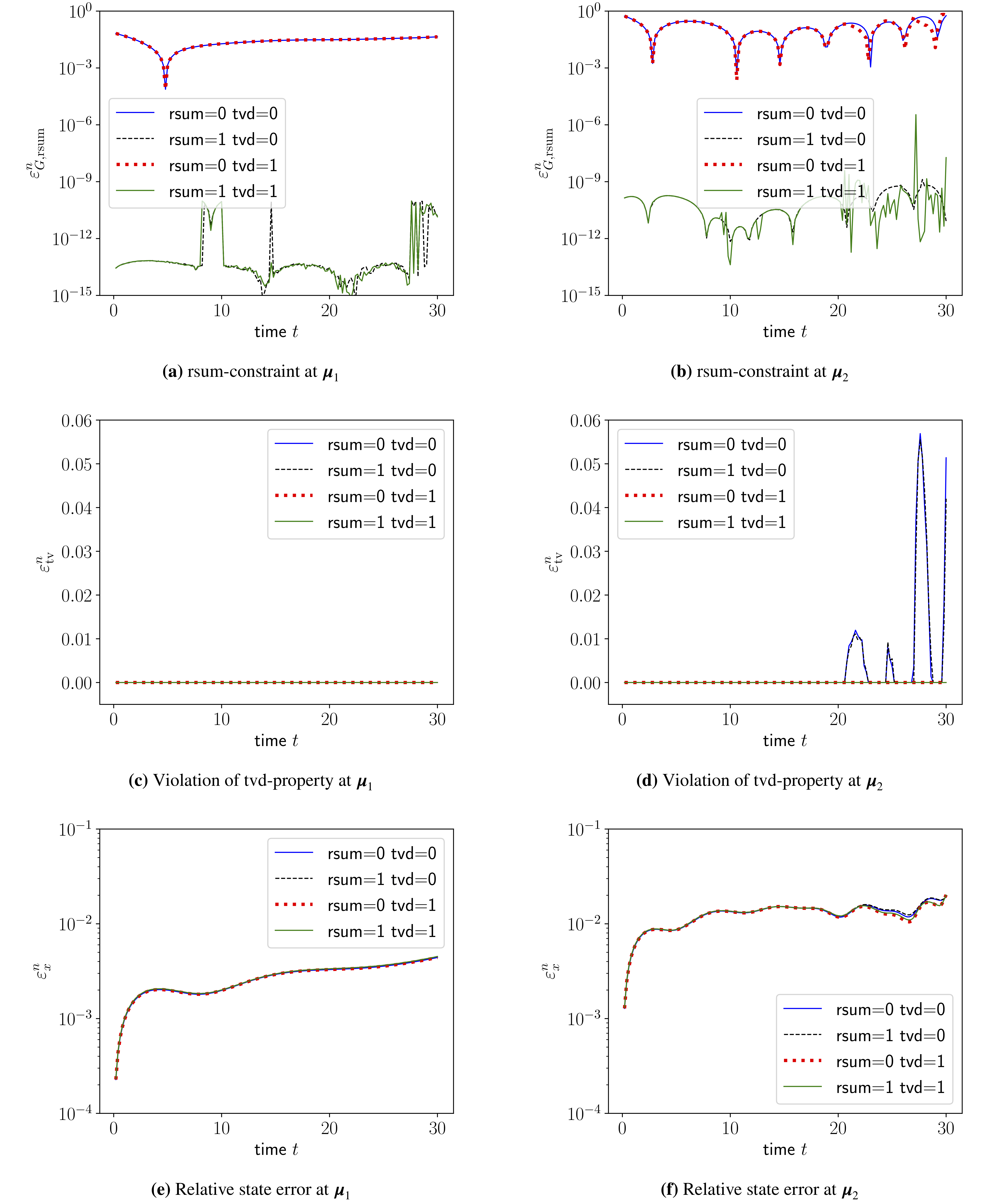
Refer to caption
Figure 5: 1D Burgers’ equation. Error metrics for the Galerkin projection (10 degrees of freedom) evaluated at 𝝁1=(0.9,0.3)subscript𝝁10.90.3{\boldsymbol{\mu}}_{1}=(0.9,0.3) and 𝝁2=(1.3,0.7)subscript𝝁21.30.7{\boldsymbol{\mu}}_{2}=(1.3,0.7). rsum = 0/1 and tvd = 0/1 denote the sum-of-residual-entries constraint and total variation diminishing constraint being not in use / in use.
Refer to caption
Figure 6: 1D Burgers’ equation. Error metrics for the LSPG projection (10 degrees of freedom) evaluated at 𝝁1=(0.9,0.3)subscript𝝁10.90.3{\boldsymbol{\mu}}_{1}=(0.9,0.3) and 𝝁2=(1.3,0.7)subscript𝝁21.30.7{\boldsymbol{\mu}}_{2}=(1.3,0.7). rsum = 0/1 and tvd = 0/1 denote the sum-of-residual-entries constraint and total variation diminishing constraint being not in use / in use.
Refer to caption
Figure 7: 1D Burgers’ equation. Galerkin projection (left column) and LSPG projection (right column) global error metrics over variable reduced-order basis size evaluated at 𝝁2=(1.3,0.7)subscript𝝁21.30.7{\boldsymbol{\mu}}_{2}=(1.3,0.7). rsum = 0/1 and tvd = 0/1 denote the sum-of-residual-entries constraint and total variation diminishing constraint being not in use / in use.

Appendix B Euler equations

Refer to caption
Figure 8: 1D Euler equations. State errors for Galerkin projection (20 degrees of freedom) evaluated at 𝝁=(1.25,1.5)𝝁1.251.5{\boldsymbol{\mu}}=(1.25,1.5). Left column plots were produced with 200 time steps and right column plots with 600 time steps. tvb = 0/1 denotes the total variation bounding constraint being not in use / in use. Unconstrained GP and LSPG are equivalent due to explicit discretization in time.
Refer to caption
Figure 9: 1D Euler equations. State total variations for Galerkin projection (GP) and LSPG projection (LSPG) (20 degrees of freedom) evaluated at 𝝁=(1.25,1.5)𝝁1.251.5{\boldsymbol{\mu}}=(1.25,1.5). Left column plots were produced with 200 time steps and right column plots with 600 time steps. tvb = 0/1 denotes the total variation bounding constraint being not in use / in use. Unconstrained GP and LSPG are equivalent due to explicit discretization in time.
Refer to caption
Figure 10: 1D Euler equations. Galerkin projection (GP) and LSPG projection (LSPG) global state errors (left column) and mean global total variation bounding constraint violation (right column) at 600 time steps. tvb = 0/1 denotes the total variation bounding constraint being not in use / in use. The unconstrained projection ROM (tvb=0) was unstable for p=40𝑝40p=40. Unconstrained GP and LSPG are equivalent due to explicit discretization in time.

Appendix C Diffusion equation

Refer to caption
Figure 11: 2D diffusion problem. Error metrics for the Galerkin projection (left column plots) and LSPG projection (right column plots) (10 degrees of freedom) evaluated at 𝝁=(106,106,104,0.2)𝝁superscript106superscript106superscript1040.2{\boldsymbol{\mu}}=(10^{6},-10^{6},10^{-4},0.2) with 100 time steps. rsum = 0/1 and ec = 0/1 denote the sum-of-residual-entries constraint and energy conservation constraint being not in use / in use.
Refer to caption
Figure 12: 2D diffusion problem. Galerkin projection (left column) and LSPG projection (right column) global error metrics over variable basis size evaluated at 𝝁=(106,106,104,0.2)𝝁superscript106superscript106superscript1040.2{\boldsymbol{\mu}}=(10^{6},-10^{6},10^{-4},0.2) with 100 time steps . rsum = 0/1 and ec = 0/1 denote the sum-of-residual-entries constraint and energy conservation constraint being not in use / in use. The simulation rsum=1, ec=1, p=5𝑝5p=5 in case of the LSPG projection failed to converge and is therefore not depicted.

Appendix D Problem-specific constraints

nomenclature interpretation constraint reference
𝜽𝜽\displaystyle{\boldsymbol{\theta}} :discretized temperature field:absentdiscretized temperature field\displaystyle:\text{discretized temperature field}  θl subscript𝜃𝑙\displaystyle \theta_{l} :lower temperature bound:absentlower temperature bound\displaystyle:\text{lower temperature bound}  θu subscript𝜃𝑢\displaystyle \theta_{u} :upper temperature bound:absentupper temperature bound\displaystyle:\text{upper temperature bound} bounded temperature to physical range min(𝜽)θl0𝜽subscript𝜃𝑙0\displaystyle\min({\boldsymbol{\theta}})-\theta_{l}\geq 0 θumax(𝜽)0subscript𝜃𝑢𝜽0\displaystyle\theta_{u}-\max({\boldsymbol{\theta}})\geq 0 Ref. [15]
𝑪¯¯𝑪\displaystyle{\bar{\boldsymbol{C}}} :subdomain conservation matrix:absentsubdomain conservation matrix\displaystyle:\ \text{subdomain conservation matrix} 𝒓𝒓\displaystyle{\boldsymbol{r}} :time-continuous  residual:absenttime-continuous  residual\displaystyle:\ \text{time-continuous \ residual}  𝒓n superscript𝒓𝑛\displaystyle {\boldsymbol{r}}^{n} :time-discrete residual:absenttime-discrete residual\displaystyle:\ \text{time-discrete residual} conservation in finite-volume models 𝑪¯𝒓¯𝑪𝒓\displaystyle{\bar{\boldsymbol{C}}}{\boldsymbol{r}} =𝟎absent0\displaystyle={\boldsymbol{0}} 𝑪¯𝒓n¯𝑪superscript𝒓𝑛\displaystyle{\bar{\boldsymbol{C}}}{\boldsymbol{r}}^{n} =𝟎absent0\displaystyle={\boldsymbol{0}} Ref. [8]
CL,(target)subscript𝐶𝐿target\displaystyle C_{L,(\mathrm{target})} :(target)liftcoefficient:absenttargetliftcoefficient\displaystyle:\mathrm{(target)\ lift\ coefficient} CD,(target)subscript𝐶𝐷target\displaystyle C_{D,(\mathrm{target})} :(target)dragcoefficient:absenttargetdragcoefficient\displaystyle:\mathrm{(target)\ drag\ coefficient} fulfillment of aerodynamic constraints CLCL,targetsubscript𝐶𝐿subscript𝐶𝐿target\displaystyle C_{L}-C_{L,\mathrm{target}} =0absent0\displaystyle=0 CDCD,targetsubscript𝐶𝐷subscript𝐶𝐷target\displaystyle C_{D}-C_{D,\mathrm{target}} =0absent0\displaystyle=0 Ref. [32]
𝝀::𝝀absent\displaystyle{\boldsymbol{\lambda}}: Lagrange multipliers (in solid mechanics contact problem) positivity of contact forces in solid mechanics contact problem 𝝀𝟎𝝀0{\boldsymbol{\lambda}}\geq{\boldsymbol{0}} Ref. [4]
K𝐾\displaystyle K :kinetic energy:absentkinetic energy\displaystyle:\text{kinetic energy} 𝒖𝒖\displaystyle{\boldsymbol{u}} :velocity field:absentvelocity field\displaystyle:\text{velocity field} ν𝜈\displaystyle\nu :kinematic viscosity:absentkinematic viscosity\displaystyle:\text{kinematic viscosity} kinetic energy balance in incompressible flows (under given modeling assumptions, see Ref. [29]) dKdt+ν𝒖2=0𝑑𝐾𝑑𝑡𝜈superscriptdelimited-∥∥𝒖20\frac{dK}{dt}+\nu\left\lVert\nabla{\boldsymbol{u}}\right\rVert^{2}=0 Ref. [29]
𝒙^lsubscript^𝒙𝑙\displaystyle{\hat{\boldsymbol{x}}}_{l} :lower bounds on generalized coordinates:absentlower bounds on generalized coordinates\displaystyle:\ \text{lower bounds on generalized coordinates} 𝒙^usubscript^𝒙𝑢\displaystyle{\hat{\boldsymbol{x}}}_{u} :upper bounds on generalized coordinates:absentupper bounds on generalized coordinates\displaystyle:\ \text{upper bounds on generalized coordinates} bounded ROM solution by hyper-parameters estimated from FOM 𝒙^𝒙^l^𝒙subscript^𝒙𝑙\displaystyle{\hat{\boldsymbol{x}}}-{\hat{\boldsymbol{x}}}_{l} 𝟎absent0\displaystyle\geq{\boldsymbol{0}} 𝒙^u𝒙^subscript^𝒙𝑢^𝒙\displaystyle{\hat{\boldsymbol{x}}}_{u}-{\hat{\boldsymbol{x}}} 𝟎absent0\displaystyle\geq{\boldsymbol{0}} Ref. [14]
Table 2: Examples for constraints (with references) representable by the general constraint set (16) - (19). Note, that the constraint on bounded generalized coordinates (last row) is not directly representable by our general constraint set, which is defined independently from the ROM solution. We nevertheless include the constraint on bounded generalized coordinates, recalling that the generalized coordinates are expressible in terms of the FOM state 𝒙^=𝚽T(𝒙𝒙ref(𝝁))^𝒙superscript𝚽𝑇𝒙subscript𝒙ref𝝁{\hat{\boldsymbol{x}}}={\boldsymbol{\Phi}}^{T}({\boldsymbol{x}}-\boldsymbol{x}_{\mathrm{ref}}({\boldsymbol{\mu}})).