Simulation-efficient marginal posterior estimation with swyft: stop wasting your precious time

Abstract

We present algorithms (a) for nested neural likelihood-to-evidence ratio estimation, and (b) for simulation reuse via an inhomogeneous Poisson point process cache of parameters and corresponding simulations. Together, these algorithms enable automatic and extremely simulator efficient estimation of marginal and joint posteriors. The algorithms are applicable to a wide range of physics and astronomy problems and typically offer an order of magnitude better simulator efficiency than traditional likelihood-based sampling methods. Our approach is an example of likelihood-free inference, thus it is also applicable to simulators which do not offer a tractable likelihood function. Simulator runs are never rejected and can be automatically reused in future analysis. As functional prototype implementation we provide the open-source software package swyft.

1 Introduction

Parametric stochastic simulators are ubiquitous in the physical sciences [1, 2, 3]. However, performing parameter inference based on simulator runs using Markov chain Monte Carlo is inconvenient or even impossible if the model parameter space is large or the likelihood function is intractable. This problem is addressed by so-called likelihood-free inference [4] or simulation-based inference [5, 6, 7, 8, 9] techniques. Among those, sequential neural ratio estimation based on amortized approximate likelihood-to-evidence ratios (SNRE-AALR) [7] is closest to our method.

We propose Nested Ratio Estimation (NRE), which approximates the likelihood-to-evidence ratio in a sequence of rounds. Loosely inspired by the contour sorting method of nested sampling [10, 11, 12], the scheme alternates between sampling from a constrained prior and estimating likelihood-to-evidence ratios. It allows for efficient estimation of any marginal posteriors of interest. Furthermore, we propose an algorithm that we call iP3 sample caching, which facilitates simulator efficiency by automatizing the reuse of previous simulator runs through resampling of cached simulations.

The primary use case for these algorithms is the calculation of arbitrary, low-dimensional marginal posteriors, typically in one or two dimensions. In physics and astronomy, such marginals serve as the basis for scientific conclusions by constraining individual model parameters within uncertainty bounds. We implement a multi-target training regime where all marginal posteriors of interest can be learned simultaneously. We find that learning is simplified when one calculates each marginal distribution directly rather than computing the full joint posterior and marginalizing numerically. Furthermore, the method facilitates effortless marginalization over arbitrary numbers of nuisance parameters, increasing its utility in high-dimensional parameter regimes–even to simulators with a tractable, yet high-dimensional, likelihood [13].

2 Proposed methods

Nested Ratio Estimation (NRE).

We operate in the context of simulation-based inference where our simulator $\mathbf{g}$ is a nonlinear function mapping a vector of parameters $\boldsymbol{\theta}=(\theta_{1},\dots,\theta_{d})\in\mathbb{R}^{d}$ and a stochastic latent state $\mathbf{z}$ to an observation $\mathbf{x}=\mathbf{g}(\boldsymbol{\theta},\mathbf{z})$. The likelihood function is therefore $p(\mathbf{x}|\boldsymbol{\theta})=\int\delta(\mathbf{x}-\mathbf{g}(\boldsymbol{\theta},\mathbf{z}))\,p(\mathbf{z}|\boldsymbol{\theta})\,d\mathbf{z}$, with $\delta(\cdot)$ denoting the Dirac delta. Consider a factored prior $p(\boldsymbol{\theta})=p_{1}(\theta_{1})\cdots p_{d}(\theta_{d})$ over the parameters, the joint posterior is given via Bayes’ rule as $p(\boldsymbol{\theta}|\mathbf{x})=p(\mathbf{x}|\boldsymbol{\theta})p(\boldsymbol{\theta})/p(\mathbf{x})$, where $p(\mathbf{x})$ is the evidence.

Our goal is to compute the marginal posterior, $p(\boldsymbol{\vartheta}|\mathbf{x})$, where $\boldsymbol{\vartheta}$ are the parameters of interest. We denote all other parameters by $\boldsymbol{\eta}$, such that $\boldsymbol{\theta}=(\boldsymbol{\vartheta},\boldsymbol{\eta})$. The marginal posterior is obtained from the joint distribution $p(\boldsymbol{\vartheta},\boldsymbol{\eta}|\mathbf{x})\equiv p(\boldsymbol{\theta}|\mathbf{x})$ by integrating over all components of $\boldsymbol{\eta}$,

$$p(\boldsymbol{\vartheta}|\mathbf{x})\equiv\int p(\boldsymbol{\vartheta},\boldsymbol{\eta}|\mathbf{x})d\boldsymbol{\eta}=\int\frac{p(\mathbf{x}|\boldsymbol{\vartheta},\boldsymbol{\eta})}{p(\mathbf{x})}p(\boldsymbol{\theta})d\boldsymbol{\eta}=\frac{p(\mathbf{x}|\boldsymbol{\vartheta})}{p(\mathbf{x})}p(\boldsymbol{\vartheta})\;,$$ (1)

where we used Bayes’ rule and defined the marginal likelihood $p(\mathbf{x}|\boldsymbol{\vartheta})$ in the last step.

Just like in SNRE-AALR, we focus on a specific observation of interest, $\mathbf{x}_{0}$. Only parameter values $\boldsymbol{\theta}$ that could have plausibly generated observation $\mathbf{x}_{0}$ will significantly contribute to the integrals in Eq. (1). For implausible values the likelihood $p(\mathbf{x}_{0}|\boldsymbol{\theta})$ will be negligible. We denote priors that are suitably constrained to plausible parameter values by $\tilde{p}(\theta_{1},\dots,\theta_{d})$. Similarly, $\tilde{\square}$ indicates quantities $\square$ that are calculated using the constrained prior. Therefore, a judiciously chosen constrained prior, accurately approximates the marginal posterior in place of our true prior beliefs,

$$p(\boldsymbol{\vartheta}|\mathbf{x}_{0})=\frac{p(\mathbf{x}_{0}|\boldsymbol{\vartheta})}{p(\mathbf{x}_{0})}p(\boldsymbol{\vartheta})\simeq\frac{\tilde{p}(\mathbf{x}_{0}|\boldsymbol{\vartheta})}{\tilde{p}(\mathbf{x}_{0})}\tilde{p}(\boldsymbol{\vartheta})\;.$$ (2)

The increased probability that constrained priors assign to the plausible parameter region cancels when dividing by the constrained evidence $\tilde{p}(\mathbf{x})$. We define the marginal likelihood-to-evidence ratio

$$\tilde{r}(\mathbf{x},\boldsymbol{\vartheta})\equiv\frac{\tilde{p}(\mathbf{x}|\boldsymbol{\vartheta})}{\tilde{p}(\mathbf{x})}=\frac{\tilde{p}(\mathbf{x},\boldsymbol{\vartheta})}{\tilde{p}(\mathbf{x})\tilde{p}(\boldsymbol{\vartheta})}=\frac{\tilde{p}(\boldsymbol{\vartheta}|\mathbf{x})}{\tilde{p}(\boldsymbol{\vartheta})}\;,$$ (3)

which is sufficient to evaluate the marginal posterior in Eq. (1), and which we will now estimate. Under the assumption of equal class population, it is known [7, 14] that one can recover density ratios using binary classification to distinguish between samples from two distributions. Our binary classification problem is to distinguish positive samples, $(\mathbf{x},\boldsymbol{\vartheta})\sim\tilde{p}(\mathbf{x},\boldsymbol{\vartheta})=p(\mathbf{x}|\boldsymbol{\vartheta})\tilde{p}(\boldsymbol{\vartheta})$, drawn jointly, and negative samples, $(\mathbf{x},\boldsymbol{\vartheta})\sim\tilde{p}(\mathbf{x})\tilde{p}(\boldsymbol{\vartheta})$, drawn marginally. The binary classifier $\sigma(f_{\phi}(\mathbf{x},\boldsymbol{\vartheta}))$ performs optimally when $f_{\phi}(\mathbf{x},\boldsymbol{\vartheta})=\log\tilde{r}(\mathbf{x},\boldsymbol{\vartheta})$, where $\sigma(\cdot)$ is the sigmoid function and $f_{\phi}$ is a neural network parameterized by $\phi$. The associated binary cross-entropy loss function [7] used to train the ratio $\tilde{r}(\boldsymbol{\vartheta},\mathbf{x}_{0})$ via stochastic gradient descent is given by

$$\ell=-\int\left[\tilde{p}(\mathbf{x}|\boldsymbol{\vartheta})\tilde{p}(\boldsymbol{\vartheta})\ln\sigma(f_{\phi}(\mathbf{x},\boldsymbol{\vartheta}))+\tilde{p}(\mathbf{x})\tilde{p}(\boldsymbol{\vartheta})\ln\sigma(-f_{\phi}(\mathbf{x},\boldsymbol{\vartheta}))\right]d\mathbf{x}\,d\boldsymbol{\vartheta}\;.$$ (4)

We propose to iteratively improve marginal posterior estimates in $R$ rounds by employing posterior estimates from previous rounds to define constrained priors. In each round $r$, we estimate all 1-dim marginal posteriors, using $d$ instances of the above marginal likelihood-to-evidence ratio estimation in parallel by setting $\boldsymbol{\vartheta}=(\theta_{i})$ for $i=1,\dots,d$. To this end, we utilize the factorized constrained prior, $\tilde{p}^{(r)}(\boldsymbol{\theta})=\tilde{p}^{(r)}_{1}(\theta_{1})\cdots\tilde{p}^{(r)}_{d}(\theta_{d})$, which is defined recursively by a cutoff criterion,

$$\tilde{p}^{(r)}_{i}(\theta_{i})\propto p_{i}(\theta_{i})\Theta_{H}\left[\frac{\tilde{r}^{(r-1)}_{i}(\mathbf{x},\theta_{i})}{\max_{\theta_{i}}\tilde{r}^{(r-1)}_{i}(\mathbf{x},\theta_{i})}-\epsilon\right],$$ (5)

where $\Theta_{H}$ denotes the Heaviside step function and $\epsilon$ denotes the minimum likelihood-ratio which passes through the threshold. We use $\tilde{p}^{(1)}(\boldsymbol{\theta})=p(\boldsymbol{\theta})$ as an initial prior in the iterative scheme.

In every round, each 1-dim posterior approximates a marginalization of the same underlying constrained posterior, allowing us to effectively reuse training data and train efficiently in a multi-target regime. The inference network is therefore divided into a featurizer $\mathbf{F}(\mathbf{x})$ with shared parameters and a set of $d$ independent Multi-layer Perceptons $\{\textrm{MLP}_{i}(\cdot,\cdot)\}_{i=1}^{d}$ which estimate individual 1-dim marginal posterior-to-prior ratios and do not share parameters, such that $f_{\phi,i}(\mathbf{x},\theta_{i})=\textrm{MLP}_{i}(\mathbf{F}(\mathbf{x}),\theta_{i})$. We estimate every 1-dim marginal simultaneously by concatenating the output of the classifiers such that $\mathbf{f}_{\phi}=(f_{\phi,1},\dots,f_{\phi,d})$.

This technique is valid as long as the excluded prior regions do not significantly affect the integrals in Eq. (1). For uncorrelated parameters, a sufficient criterion is that the impact on the marginal posteriors is small, which we guarantee through the iteration criterion Eq. (5). In the case of a very large number of strongly correlated parameters the algorithm can inadvertently cut away tails of the marginal posteriors. Decreasing $\epsilon$ mitigates this effect. Discussion is left for future study.

With this design, the posteriors from the final round can be used as an approximation of the true 1-dim marginal posteriors, $\tilde{p}^{(R)}(\theta_{i}|\mathbf{x}_{0})\approx p(\theta_{i}|\mathbf{x}_{0})$, while previous rounds were used to iteratively focus on relevant parts of the parameter space. The key result and value of NRE lies in the utility of our constrained prior from round $R$. The final constrained prior, $\tilde{p}^{(R)}(\boldsymbol{\theta})$, along with previously generated and cached samples, allows for estimation of any higher dimensional marginal posterior $\tilde{p}^{(R)}(\boldsymbol{\vartheta}|\mathbf{x}_{0})\approx p(\boldsymbol{\vartheta}|\mathbf{x}_{0})$ of interest by doing likelihood-to-evidence ratio estimation. The NRE algorithm is detailed in the supplementary material.

Inhomogeneous Poisson Point Process (iP3) Sample Caching.

Simulating $(\mathbf{x},\boldsymbol{\theta})\sim p(\mathbf{x}|\boldsymbol{\theta})p(\boldsymbol{\theta})$ can be extremely expensive. We develop a scheme to systematically reuse appropriate subsets of previous simulator runs. Our method samples $N\sim\text{Pois}(\hat{N})$ parameter vectors from an arbitrary distribution $p(\boldsymbol{\theta})$, where $\hat{N}$ is the expected number of samples. Taking $N$ samples from $p(\boldsymbol{\theta})$ is equivalent to drawing a single sample $\Theta\equiv\{\boldsymbol{\theta}^{(n)}\}_{n=1}^{N}$ from an inhomogenous Poisson point process (PPP) with intensity function $\lambda(\boldsymbol{\theta})=\hat{N}p(\boldsymbol{\theta})$. In this context, $\Theta$ is known as a set of points. This formulation provides convenient mathematical properties [15], at the low price of introducing variance in the number of samples drawn. The precise number of samples does not matter as long as $N\approx\hat{N}$, which is true in our regime of order $\geq 1000$.

We will need two properties of PPPs. Superposition: Given two independent PPPs with intensity functions $\lambda_{1}(\boldsymbol{\theta})$ and $\lambda_{2}(\boldsymbol{\theta})$, the sum yields another PPP with intensity function $\lambda(\boldsymbol{\theta})=\lambda_{1}(\boldsymbol{\theta})+\lambda_{2}(\boldsymbol{\theta})$. The union of two sets of points $\Theta=\Theta_{1}\cup\Theta_{2}$ from the individual PPPs is equivalent to a single set of points from the combined PPP. Thinning: Consider a PPP with intensity function $\lambda(\boldsymbol{\theta})$, and an arbitrary function $q(\boldsymbol{\theta}):\mathbb{R}^{d}\to[0,1]$. If we are interested in drawing from a PPP with intensity function $\lambda_{q}(\boldsymbol{\theta})=q(\boldsymbol{\theta})\lambda(\boldsymbol{\theta})$, we can achieve this by drawing a set of points $\Theta$ distributed like $\lambda(\boldsymbol{\theta})$ and then rejecting individual points $\boldsymbol{\theta}^{(n)}$ with probability $1-q(\boldsymbol{\theta}^{(n)})$.

We define a parameter cache by a set of points $\Theta_{sc}$ drawn from a PPP with intensity function $\lambda_{sc}(\boldsymbol{\theta})$. For every point $\boldsymbol{\theta}\in\Theta_{sc}$, a corresponding observation $\mathbf{x}$ is stored in an observation cache $\mathcal{X}_{sc}$. Our iP3 cache sampling algorithm that is responsible for maintaining the caches and sampling from a PPP with target intensity function $\lambda_{t}(\boldsymbol{\theta})=\hat{N}p(\boldsymbol{\theta})$ is written out in the supplementary material. It is summarized in two steps: First, consider all points $\boldsymbol{\theta}\in\Theta_{sc}$ from the cache and accept them with probability $\min(1,\lambda_{t}(\boldsymbol{\theta})/\lambda_{sc}(\boldsymbol{\theta}))$. The thinning operation yields a sample $\Theta_{1}$ from a PPP with intensity function $\lambda_{1}(\boldsymbol{\theta})=\min(\lambda_{t}(\boldsymbol{\theta}),\lambda_{sc}(\boldsymbol{\theta}))$. Second, draw a new set of points $\Theta_{p}$ from $\lambda_{t}(\boldsymbol{\theta})$, and accept each $\boldsymbol{\theta}\in\Theta_{p}$ with probability $\max(0,1-\lambda_{sc}(\boldsymbol{\theta})/\lambda_{t}(\boldsymbol{\theta}))$. This yields a sample $\Theta_{2}$ from a PPP with intensity function $\lambda_{2}(\boldsymbol{\theta})=\max(0,\lambda_{t}(\boldsymbol{\theta})-\lambda_{sc}(\boldsymbol{\theta}))$. Thanks to superposition, the union $\Theta_{1}\cup\Theta_{2}=\Theta_{t}$ yields a sample from the PPP with intensity function $\lambda_{t}(\boldsymbol{\theta})$–the sample we were looking for. We only need to run simulations on points from $\Theta_{1}$. Points in $\Theta_{2}$ already have corresponding observations in $\mathcal{X}_{sc}$ which we can reuse. Finally, the new parameters are appended to the set of points in the parameter cache, $\Theta_{sc}\to\Theta_{sc}\cup\Theta_{2}$. Similar for $\mathcal{X}_{sc}$. On the basis of the superposition principle, the intensity function of the $\Theta_{sc}$ cache is updated $\lambda_{sc}(\boldsymbol{\theta})\to\max(\lambda_{sc}(\boldsymbol{\theta}),\lambda_{t}(\boldsymbol{\theta}))$.

Storing and updating the parameter cache’s intensity function $\lambda_{sc}(\boldsymbol{\theta})$ can pose challenges when it is complex and high-dimensional. Our NRE implementation overcomes these challenges by learning marginal 1-dim posteriors, guaranteeing that the relevant target intensities always factorize, $\lambda_{t}(\boldsymbol{\theta})=\lambda_{t}(\theta_{1})\cdots\lambda_{t}(\theta_{d})$. Storage of and calculation with factorizable functions simplifies matters.

3 Experiments and discussion

Although NRE is applicable to scenarios where the likelihood is intractable, we focus on examples with tractable likelihoods in order to compare our results with the ground truth obtained by sampling techniques. In this case, ground truth results are provided by MultiNest [11, 16], a nested sampling tool widely used in the physics and astronomy community. Examples are of illustrative nature, a quantitative comparison between methods will be left for future study.

Experiments.

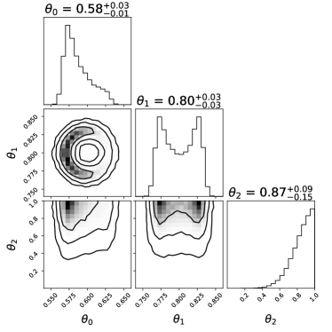
Consider a simulator $g(\boldsymbol{\theta},\mathbf{z})=(\theta_{0},\sqrt{(\theta_{0}-0.6)^{2}+(\theta_{1}-0.8)^{2}},\theta_{2})+\textbf{n}$, where n is drawn from a zero-mean multivariate Gaussian distribution with a diagonal covariance matrix, $\boldsymbol{\Sigma}=\textrm{diag}(0.03,0.005,0.2)$. The first task was to infer $\boldsymbol{\theta}$ for synthetic data generated by ground truth parameters $\boldsymbol{\theta}=(0.57,0.8,1.0)$. In our reported estimates, as seen in Fig. 1, MultiNest required 160722 simulations, while NRE obtained comparable marginal posteriors after only 20011 simulations divided across four rounds. A visualization of the cache $\Theta_{sc}$, utilized in NRE over four rounds, is presented in the supplementary material (see Fig.  3). The second task was to infer new parameters $\boldsymbol{\theta}=(0.55,0.8,1.0)$ with the same simulator. MultiNest required 171209 new simulator runs while iP3 sample caching reduced the number of additionally required simulator runs to only 3668 when performing NRE. NRE is efficient initially and enables hyper-efficient follow up studies.

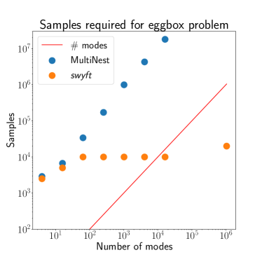
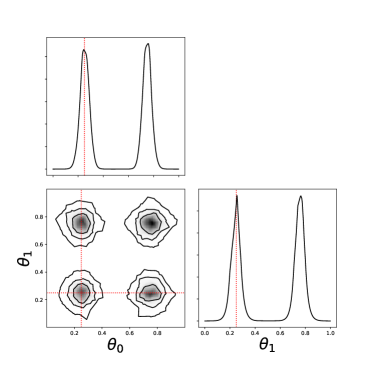
In our second experiment, the simulator gives rise to an “eggbox” posterior, with modes at $\theta_{i}=0.5\pm 0.25$, $i=0,\dots d-1$. The simulation model is $g_{i}(\boldsymbol{\theta},\mathbf{z})=\sin(\theta_{i}\cdot\pi)+n_{i}$, where $\mathbf{n}$ is a zero-mean Gaussian noise with standard deviation 0.1. For this model, the number of modes grows exponentially with the dimension of $\boldsymbol{\theta}$ as $2^{d}$. As such, the number of samples required for MultiNest scales exponentially with the dimension and quickly becomes infeasible, see Fig. 2. At $d=20$ there are over $10^{6}$ modes and MultiNest cannot solve the problem before memory constraints take over. We find that, with standard settings, MultiNest requires at least $10^{7}$ samples for $d=14$ to give reasonable results (which corresponds to $\sim 10^{3}$ samples per mode). On the other hand, our proposed method directly estimates marginal posteriors at almost constant simulator cost, with $2\times 10^{4}$ samples sufficient even for $d=20$ (much less than one sample per mode). Since we focus with NRE directly on marginal posteriors, resolving the exponentially large number of modes becomes unnecessary.

[]table[0.4] NRE/iP3 MultiNest Run 1 20011 160722 Run 2 3668 171209

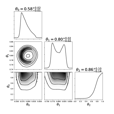
Table 1: Numbers of samples required by NRE/iP3 and MultiNest for first experiment. We infer posteriors for two instances of the problem. In the second instance, NRE/iP3 benefits from sample reuse while MultiNest cannot reuse any parameters or simulations.

Figure 1: Marginal posteriors produced by NRE/iP3 (left) and MultiNest (right) for Run 1 of our example. The contours for $68\%,~{}95\%,$ and $99.7\%$ credible regions are shown.

Figure 2: Left: scaling of simulator cost with respect to number of modes for the eggbox problem. For MultiNest, each mode must be sampled, leading to a rapid increase in simulator cost as a function of problem dimension. On the other hand, by directly evaluating the marginal posteriors, the proposed method is able to solve the problem at almost constant computational cost. Right: posteriors computed via a network for $d=20$ trained on $2\times 10^{4}$ samples. For ease of visualization, we show only the set of 1- and 2-dimensional marginal posteriors truncated to $\theta_{0},\theta_{1}$; marginal posteriors for all other parameter pairs look similar.

Discussion.

NRE with iP3 sample caching is meant as a significantly more flexible, and simulator efficient, alternative to the likelihood-based sampling tools commonly used in physics. In the above experiment we show that – without much tuning – our algorithms achieved similar accuracy to the widely used nested sampler MultiNest while reducing simulator calls by an order of magnitude. Furthermore, analysis of similar inference problems with usual sampling tools, like MultiNest, must start from scratch and redo many simulations; however, NRE with iP3 sample caching allows us to reuse simulator runs from previous analyses to further reduce simulation costs. NRE is applicable to simulators which do not have a tractable likelihood, significantly broadening the set of use-cases.

In our reference implementation of NRE with iP3 sample caching, the initial rounds are based on simultaneous learning of one dimensional marginal posteriors, implemented efficiently via multi-target training. Once converged, higher-dimensional marginals can be scrutinized in the relevant region after training a new likelihood ratio estimator on already-collected data. Empirically, using low dimensional marginals and constraining the prior to relevant regions of parameter space reduces the difficulty of the learning problem such that relatively simple neural networks are sufficient to estimate satisfactory marginal posteriors. In future work we will consider how to further capitalize on this learning problem simplification by using higher dimensional marginal priors and posteriors during the training rounds of NRE. The aim is to improve prediction across highly correlated parameters. As a product of these efforts, we offer an open source Python package which implements NRE and iP3 sample caching called swyft. It has a convenient API for use by machine learning non-specialists.

Broader Impact

The proposed algorithms aim at facilitating solutions to the "inverse problem" for simulator-based modeling in the limit of expensive simulator runs. Although we have physics and astronomy applications in mind, the underlying problem is rather common in the quantitative sciences. For example, benchmark problems include the Lotka–Volterra predator-prey model and the m/d/1 queue problems. Therefore, the breadth use cases must be considered and the software may be used to make modeling decisions which affect the lives of humans. We do not anticipate specific cases of misuse of the methods, but emphasize that the inference method is only as good as the simulator, and limited simulation models can lead to false conclusions. A problematic failure mode would be to choose a simulator which reinforces already held biases. Our method does not absolve the scientist of the responsibility on the choice of simulator. However, our algorithms do not directly penalize model complexity, and hence allow and encourage the construction of more realistic models.

Supplementary Material

Input : Simulator $p(\mathbf{x}|\boldsymbol{\theta})$, factorizable prior $p(\boldsymbol{\theta})$, real observation $\mathbf{x}_{0}$, parameter dimension $d$, classifiers $\{f_{\phi,i}(\mathbf{x},\theta_{i})\}_{i=1}^{d}$, rounds $R$, mean samples per round $\hat{N}$, likelihood cutoff $\epsilon$.

Init: Constrained prior $p^{(1)}(\boldsymbol{\theta})=p(\boldsymbol{\theta})$, caches $\mathcal{X}_{sc},\Theta_{sc}=\{\}$, intensity function $\lambda_{sc}(\boldsymbol{\theta})=0$.

for $r=1$ to $R$ do

       Sample points using Algorithm 2, the iP3 sample caching algorithm,

       $\{(\mathbf{x}^{(n)},\boldsymbol{\theta}^{(n)})\}_{n=1}^{N\sim\text{Pois}(\hat{N})}$, $\mathcal{X}_{sc}$, $\Theta_{sc}$, $\lambda_{sc}(\boldsymbol{\theta})$ = iP3 $(p(\mathbf{x}|\boldsymbol{\theta}),\hat{N},p^{(r)}(\boldsymbol{\theta}),\mathcal{X}_{sc},\Theta_{sc},\lambda_{sc}(\boldsymbol{\theta}))$.

       (Re-) initialize $\mathbf{f}_{\phi}=(f_{\phi,i})_{i=1}^{d}$.

       while $\mathbf{f}_{\phi}$ not converged do

             Extract mini-batch $\{(\mathbf{x}^{(b)},\boldsymbol{\theta}^{(b)})\}_{b=1}^{B}\subset\{(\mathbf{x}^{(n)},\boldsymbol{\theta}^{(n)})\}_{n=1}^{N\sim\text{Pois}(\hat{N})}$, $B\equiv 0\pmod{2}$.

             Randomly pair up all samples from the mini-batch $((\mathbf{x}^{(a,0)},\boldsymbol{\theta}^{(a,0)}),(\mathbf{x}^{(a,1)},\boldsymbol{\theta}^{(a,1)}))$ where $a=1,\dots,B/2$.

             Minimize $\mathcal{L}(\phi)=-\frac{1}{B}\sum_{a=1}^{B/2}\sum_{i=1}^{d}\sum_{j\in\{0,1\}}\sigma(f_{\phi,i}(\mathbf{x}^{(a,j)},\theta_{i}^{(a,j)}))+\sigma(-f_{\phi,i}(\mathbf{x}^{(a,j)},\theta_{i}^{(a,\neg j)}))$ using stochastic gradient descent or a variant.

            

       end while

      Constrain $p^{(r+1)}_{i}(\theta_{i})\propto p_{i}(\theta_{i})\,\Theta_{H}\left[\frac{\exp(f_{\phi,i}(\mathbf{x}_{0},\theta_{i}))}{\max_{\theta_{i}}\exp(f_{\phi,i}(\mathbf{x}_{0},\theta_{i}))}-\epsilon\right]$ in order to construct constrained prior $p^{(r+1)}(\boldsymbol{\theta})=p^{(r+1)}_{1}(\theta_{1})\cdots p^{(r+1)}_{d}(\theta_{d})$.

      

end for

Algorithm 1 Nested Ratio Estimation (NRE)

Input : Simulator $p(\mathbf{x}|\boldsymbol{\theta})$, mean samples per round $\hat{N}$, constrained prior $p(\boldsymbol{\theta})$,

observation cache $\mathcal{X}_{sc}$, parameter cache $\Theta_{sc}$, intensity function $\lambda_{sc}(\boldsymbol{\theta})$.

Output : Samples $\{(\mathbf{x}^{(n)},\boldsymbol{\theta}^{(n)}):(\mathbf{x}^{(n)},\boldsymbol{\theta}^{(n)})\sim p(\mathbf{x}|\boldsymbol{\theta})p(\boldsymbol{\theta})\,\forall n\}_{n=1}^{N\sim\text{Pois}(\hat{N})}$,

observation cache $\mathcal{X}_{sc}$, parameter cache $\Theta_{sc}$, parameter cache intensity function $\lambda_{sc}(\boldsymbol{\theta})$.

Init: Number of points $N\sim\text{Pois}(\hat{N})$, size of cache $M=|\Theta_{sc}|\ =|\mathcal{X}_{sc}|$, output set $\mathcal{O}=\{\}$, target intensity function $\lambda_{t}(\boldsymbol{\theta})=\hat{N}p(\boldsymbol{\theta})$.

for $m=1$ to $M$ do

       with probability $\min(1,\lambda_{t}(\boldsymbol{\theta})/\lambda_{sc}(\boldsymbol{\theta}))$ do

             Get observation by index $\mathbf{x}^{(m)}=\mathcal{X}_{sc}^{(m)}$.

             Get parameter vector by index $\boldsymbol{\theta}^{(m)}=\Theta_{sc}^{(m)}$.

             Append sample to output set $\mathcal{O}=\mathcal{O}\cup\{(\mathbf{x}^{(m)},\boldsymbol{\theta}^{(m)})\}$.

            

       end

      

end for

for $n=1$ to $N$ do

       Draw parameter sample $\boldsymbol{\theta}^{(n)}\sim p(\boldsymbol{\theta})$.

       with probability $\max(0,1-\lambda_{sc}(\boldsymbol{\theta})/\lambda_{t}(\boldsymbol{\theta}))$ do

             Simulate $\mathbf{x}^{(n)}\sim p(\mathbf{x}|\boldsymbol{\theta}^{(n)})$.

             Append sample to output set $\mathcal{O}=\mathcal{O}\cup\{(\mathbf{x}^{(n)},\boldsymbol{\theta}^{(n)})\}$.

            

       end

      

end for

Update parameter cache $\Theta_{sc}=\Theta_{sc}\cup\{\boldsymbol{\theta}^{(n)}\}_{n=1}^{|\mathcal{O}|\sim\text{Pois}(\hat{N})}$.

Update observation cache $\mathcal{X}_{sc}=\mathcal{X}_{sc}\cup\{\mathbf{x}^{(n)}\}_{n=1}^{|\mathcal{O}|\sim\text{Pois}(\hat{N})}$. (Note, both caches are sets indexed by the order in which elements were added to them. Duplicate elements are ignored.)

Update intensity function of parameter cache $\lambda_{sc}(\boldsymbol{\theta})=\max(\lambda_{sc}(\boldsymbol{\theta}),\lambda_{t}(\boldsymbol{\theta}))$.

return $\mathcal{O}$, $\mathcal{X}_{sc}$, $\Theta_{sc}$, $\lambda_{sc}(\boldsymbol{\theta})$.

Algorithm 2 Inhomogeneous Poisson Point Process (iP3) Sample Caching

Figure 3: Parameter cache $\Theta_{sc}$ contents for our first experiments. (See Table 1.) Samples added in the first and second runs are shown in blue and orange, respectively. The second run reuses samples computed during the first run. The evolution of the cache towards relevant parameter regimes is visible.

References

• [1] Nilanjan Banik, Gianfranco Bertone, JoΒ Bovy, and Nassim Bozorgnia. Probing the nature of dark matter particles with stellar streams. Journal of Cosmology and Astroparticle Physics, 2018(07):061–061, Jul 2018.
• [2] Richard Bartels, Suraj Krishnamurthy, and Christoph Weniger. Strong support for the millisecond pulsar origin of the galactic center gev excess. Physical Review Letters, 116(5), Feb 2016.
• [3] Aldo RodrΓ­guez-Puebla, Peter Behroozi, Joel Primack, Anatoly Klypin, Christoph Lee, and Doug Hellinger. Halo and subhalo demographics with planck cosmological parameters: Bolshoi–planck and multidark–planck simulations. Monthly Notices of the Royal Astronomical Society, 462(1):893–916, Jul 2016.
• [4] ScottΒ A Sisson, Yanan Fan, and Mark Beaumont. Handbook of approximate Bayesian computation. CRC Press, 2018.
• [5] George Papamakarios, David Sterratt, and Iain Murray. Sequential neural likelihood: Fast likelihood-free inference with autoregressive flows. In The 22nd International Conference on Artificial Intelligence and Statistics, pages 837–848. PMLR, 2019.
• [6] David Greenberg, Marcel Nonnenmacher, and Jakob Macke. Automatic posterior transformation for likelihood-free inference. In Proceedings of the 36th International Conference on Machine Learning, 2019.
• [7] Joeri Hermans, Volodimir Begy, and Gilles Louppe. Likelihood-free mcmc with amortized approximate ratio estimators. arXiv preprint arXiv:1903.04057, 2019.
• [8] Kyle Cranmer, Johann Brehmer, and Gilles Louppe. The frontier of simulation-based inference. Proceedings of the National Academy of Sciences, 2020.
• [9] Conor Durkan, Iain Murray, and George Papamakarios. On contrastive learning for likelihood-free inference. arXiv preprint arXiv:2002.03712, 2020.
• [10] John Skilling. Nested sampling for general bayesian computation. Bayesian Anal., 1(4):833–859, December 2006.
• [11] FΒ Feroz, MΒ P Hobson, and MΒ Bridges. MultiNest: an efficient and robust bayesian inference tool for cosmology and particle physics. Mon. Not. Roy. Astron. Soc. 398: 1601-1614,2009, September 2008.
• [12] WΒ J Handley, MΒ P Hobson, and AΒ N Lasenby. polychord : next-generation nested sampling. Mon. Not. R. Astron. Soc., 453(4):4384–4398, September 2015.
• [13] Adam Coogan, Konstantin Karchev, and Christoph Weniger. Targeted likelihood-free inference of dark matter substructure in strongly-lensed galaxies. arXiv preprint arXiv:2010.07032, 2020.
• [14] Kyle Cranmer, Juan Pavez, and Gilles Louppe. Approximating likelihood ratios with calibrated discriminative classifiers. arXiv preprint arXiv:1506.02169, 2015.
• [15] J.Β F.Β C. Kingman. Poisson Processes. Oxford University Press, 1993.
• [16] Buchner, J., Georgakakis, A., Nandra, K., Hsu, L., Rangel, C., Brightman, M., Merloni, A., Salvato, M., Donley, J., and Kocevski, D. X-ray spectral modelling of the agn obscuring region in the cdfs: Bayesian model selection and catalogue. A&A, 564:A125, 2014.
• [17] CharlesΒ R. Harris, K.Β Jarrod Millman, St’efanΒ J. vanΒ der Walt, Ralf Gommers, Pauli Virtanen, David Cournapeau, Eric Wieser, Julian Taylor, Sebastian Berg, NathanielΒ J. Smith, Robert Kern, Matti Picus, Stephan Hoyer, MartenΒ H. van Kerkwijk, Matthew Brett, Allan Haldane, JaimeΒ Fern’andez del R’ıo, Mark Wiebe, Pearu Peterson, Pierre G’erard-Marchant, Kevin Sheppard, Tyler Reddy, Warren Weckesser, Hameer Abbasi, Christoph Gohlke, and TravisΒ E. Oliphant. Array programming with NumPy. Nature, 585(7825):357–362, September 2020.
• [18] Pauli Virtanen, Ralf Gommers, TravisΒ E. Oliphant, Matt Haberland, Tyler Reddy, David Cournapeau, Evgeni Burovski, Pearu Peterson, Warren Weckesser, Jonathan Bright, StΓ©fanΒ J. van der Walt, Matthew Brett, Joshua Wilson, K.Β Jarrod Millman, Nikolay Mayorov, Andrew R.Β J. Nelson, Eric Jones, Robert Kern, Eric Larson, CΒ J Carey, Δ°lhan Polat, YuΒ Feng, EricΒ W. Moore, Jake VanderPlas, Denis Laxalde, Josef Perktold, Robert Cimrman, Ian Henriksen, E.Β A. Quintero, CharlesΒ R. Harris, AnneΒ M. Archibald, AntΓ΄nioΒ H. Ribeiro, Fabian Pedregosa, Paul van Mulbregt, and SciPy 1.0 Contributors. SciPy 1.0: Fundamental Algorithms for Scientific Computing in Python. Nature Methods, 17:261–272, 2020.
• [19] J.Β D. Hunter. Matplotlib: A 2d graphics environment. Computing in Science & Engineering, 9(3):90–95, 2007.
• [20] Adam Paszke, Sam Gross, Francisco Massa, Adam Lerer, James Bradbury, Gregory Chanan, Trevor Killeen, Zeming Lin, Natalia Gimelshein, Luca Antiga, Alban Desmaison, Andreas Kopf, Edward Yang, Zachary DeVito, Martin Raison, Alykhan Tejani, Sasank Chilamkurthy, Benoit Steiner, LuΒ Fang, Junjie Bai, and Soumith Chintala. Pytorch: An imperative style, high-performance deep learning library. In H.Β Wallach, H.Β Larochelle, A.Β Beygelzimer, F.Β dΒ AlchΓ©-Buc, E.Β Fox, and R.Β Garnett, editors, Advances in Neural Information Processing Systems 32, pages 8024–8035. Curran Associates, Inc., 2019.
• [21] Thomas Kluyver, Benjamin Ragan-Kelley, Fernando PΓ©rez, Brian Granger, Matthias Bussonnier, Jonathan Frederic, Kyle Kelley, Jessica Hamrick, Jason Grout, Sylvain Corlay, Paul Ivanov, DamiΓ‘n Avila, Safia Abdalla, Carol Willing, and Jupyter development team. Jupyter notebooks - a publishing format for reproducible computational workflows. In Fernando Loizides and Birgit Scmidt, editors, Positioning and Power in Academic Publishing: Players, Agents and Agendas, pages 87–90, Netherlands, 2016. IOS Press.