Experimental Detection of the Correlation Rényi Entropy in the Central Spin Model

Abstract

We propose and experimentally measure an entropy that quantifies the volume of correlations among qubits. The experiment is carried out on a nearly isolated quantum system composed of a central spin coupled and initially uncorrelated with 15 other spins. Due to the spin-spin interactions, information flows from the central spin to the surrounding ones forming clusters of multi-spin correlations that grow in time. We design a nuclear magnetic resonance experiment that directly measures the amplitudes of the multi-spin correlations and use them to compute the evolution of what we call correlation Rényi entropy. This entropy keeps growing even after the equilibration of the entanglement entropy. We also analyze how the saturation point and the timescale for the equilibration of the correlation Rényi entropy depend on the system size.

Which microscopic entropy can capture the changes undergone by an isolated quantum system that evolves in time? The von Neumann entropy for the entire density matrix of the system is not an appropriate choice, because it is constant in isolated systems. A common approach is to trace out part of the system and resort to the entanglement entropy, which quantifies the degree of entanglement between the traced-out part and the remaining subsystem. Despite the challenges presented by this quantity, it has been experimentally measured in a system with 3 superconducting qubits after tomographically reconstructing the evolved density matrix Neill et al. (2016), in a Bose-Hubbard system with 6 cold atoms and site-resolved number statistics Kaufman et al. (2016), and in a chain with 20 trapped ions where the entropy of subsystems with up to 10 ions is obtained through randomized measurements Brydges et al. (2019). The entanglement entropy is bounded by the quantum Fisher information. This quantity offers a way to detect the flow of information Lu et al. (2010); Gärttner et al. (2018) and has been experimentally measured with trapped ions Smith et al. (2016) and in nuclear magnetic resonance (NMR) Niknam et al. (2020).

Another entropy that has received more theoretical than experimental attention is the participation Rényi entropy, which measures the spread in time of a non-stationary state in the Hilbert space. The system is usually prepared in a certain basis vector and the entropy is computed by summing the squares (or larger powers) of the probabilities for finding the system in its initial quantum state and in each one of the other basis vectors Flambaum and Izrailev (2001). For both the participation Rényi entropy and the entanglement entropy, common questions include the conditions for linear or logarithmic growths in association with quantum chaos Asplund and Bernamonti (2014); Bianchi et al. (2018); Santos et al. (2012a); Vidmar and Rigol (2017); Borgonovi et al. (2019) or the transition to many-body localization Žnidarič et al. (2008); Bardarson et al. (2012); Torres-Herrera and Santos (2017); Lukin et al. (2019); DaumannARXIV , comparisons between their saturation values and thermodynamic entropies in studies of thermalization Santos et al. (2012b); Kaufman et al. (2016), and analytic predictions for the spread of entanglement Page (1993); Vidmar et al. (2017); Alba and Calabrese (2017); Calabrese (2020). One of the differences between the two entropies is that the participation Rényi entropy is extensive in the Hilbert space size of the composite system, while the maximum value of the entanglement entropy is not if the size of the subsystem does not change.

In this work, we propose a third alternative that we measure employing NMR techniques. NMR has been used to investigate questions in many-body quantum dynamics, such as many-body localization Wei et al. (2018), prethermalization Wei et al. (2019); Yin et al. (2020), and the scrambling of quantum information Niknam et al. (2020); Li et al. (2017); Sánchez et al. (2020). Our experiment demonstrates that NMR platforms are also testbeds for the analysis of entropy growth.

Our entropy quantifies the growth of the volume of correlations as information flows from a central spin (qubit) to its surrounding spins. As devices with ever larger numbers of qubits become operational, a detailed picture of how quantum information flows and how the dynamics saturates are essential for designing and controlling quantum processors. This understanding is also necessary for classical simulations, which become impracticable under a substantial growth of correlations.

Figure 1: Schematic illustration of the flow of information initially contained in the central spin (orange circle) to the surrounding 15 spins. Each shaded area indicates a cluster of correlated spins.

In our sample, the central spin is initially polarized and coupled with 15 unpolarized surrounding spins. This composite system is at room temperature and nearly isolated from external environments. The experiment employs two main ingredients available to solid-state NMR. One is the possibility to coherently average out the interactions among the surrounding spins, so that the remaining effective Hamiltonian contains only the interactions between those spins and the central one. Due to these couplings, as we sketch in Fig. 1, information that is initially concentrated in the central spin (orange circle) flows to the surroundings spins and give rise to clusters of multi-spin correlations (shades) that grow in time. The second important element of the experiment is the possibility to collectively rotate the spins and perform a basis transformation that allows us to monitor the growth of multi-spin correlations by probing only the central spin Ramanathan et al. (2003); Cho et al. (2005); Niknam et al. (2020).

We use the amplitudes of the multi-spin correlations to compute what we call correlation Rényi entropy. We find that after the saturation of the entanglement entropy, the correlation Rényi entropy keeps growing for times an order of magnitude longer, during which the larger clusters of multi-spin correlations build up. The experimental results show excellent agreement with our numerical simulations. We also perform a scaling analysis of the growth rate, the saturation value, and the equilibration time of the correlation Rényi entropy. Both the rate and the saturation point grow logarithmically as the size of the composite system increases, while the equilibration time is nearly independent of system size.

Experimental System.– We work with a polycrystalline solid made of an ensemble of Triphenylphosphine molecules. Each molecule has a central ³¹P nuclear spin coupled to ¹H spins via the heteronuclear dipolar interaction

$$\mathcal{H}_{\text{CS-B}}=\sum_{j}^{\text{N}}\omega_{j}\sigma_{\text{\tiny Z}}^{\text{CS}}\vbox{\hbox{$\scriptstyle\otimes$}}\sigma_{\text{\tiny Z}}^{j}\vbox{\hbox{$\scriptstyle\otimes$}}\mathds{1}^{\tiny\vbox{\hbox{$\scriptstyle\otimes$}}N-1},$$ (1)

where ‘CS’ stands for central spin, ‘B’ for the finite bath with $N=15$ surrounding spins, and $\sigma_{\text{\tiny Z}}^{j}$ is the Pauli matrix for the $j^{\text{th}}$ spin. The coupling constants $\omega_{j}$ are determined by the orientation and the distance of the bath spins from the central spin, the majority having values below 1200 Hz (see distribution in Niknam et al. (2020)).

Quantum information resides initially in the central spin, which is prepared in a polarized state $\rho^{\text{CS}}(0)=\sigma_{\text{\tiny X}}/2$  Not , while the surrounding spins are in a fully mixed state $\rho^{\text{B}}(0)=(\mathds{1}/2)^{\vbox{\hbox{$\scriptstyle\otimes$}}N}$. The homonuclear dipolar interactions among the bath spins are averaged out by applying the MREV-8 pulse sequence, which cancels the interactions up to the third order of the Magnus expansion, including pulse imperfection effects Haeberlen (1976); Rhim et al. (1973); Gerstein and Dybowski (1985). During the entire time span of our experiment, the effects of external environments are also under control Niknam et al. (2020), so that the evolution of the density matrix of the composite system, $\rho(T)=U_{\text{CS-B}}(T)\rho(0)U_{\text{CS-B}}^{\dagger}(T)$, is effectively described by the unitary propagator $U_{\text{CS-B}}(T)=\text{e}^{-i\mathcal{H}_{\tiny\text{CS-B}}T}$. As the CS-B system evolves under the ZZ interaction, information from the central spin gets shared with the bath spins giving rise to clusters of multi-spin correlations.

FID and Entanglement Entropy.– The loss of information from the central spin can be quantified with the free induction decay (FID),

$$\text{FID}(T)\!=\!\operatorname{Tr}\{\sigma_{\text{\tiny X}}^{\text{cs}}\rho^{\text{cs}}(T)\}\!=\!\frac{1}{2^{N+1}}\!\!\sum_{k=1}^{2^{N+1}}\cos(2\langle\phi_{k}|\mathcal{H}_{\text{CS-B}}|\phi_{k}\rangle t),$$ (2)

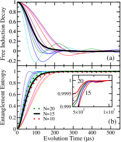
where $\rho^{\text{CS}}(T)=\operatorname{Tr}_{\text{B}}[\rho(T)]$ and $|\phi_{k}\rangle$ is one of the $2^{N+1}$ spin configurations in the $z$-direction, such as $|\uparrow\downarrow\downarrow\ldots\uparrow\rangle$. The results from numerical simulations for $N=15$ are shown in Fig. 2 (a). Thin lines correspond to representative random orientations of the molecules and the thick curve gives the average over 300 random realizations. The curve for the ensemble average is smooth and quickly saturates at $\overline{F}\sim 0$.

Figure 2: Free induction decay (a) and entanglement entropy (b) for a central spin coupled with 15 surrounding spins via the ZZ interaction in Eq. (1). Thin lines are obtained with random realizations of the coupling constants $\omega_{j}$, thick line gives the average over 300 orientations of the molecule. The dotted lines in (b) give the ensemble average for $N=10$ and $N=20$. Inset of panel (b): Averaged entangled entropy for $N=15,16,\ldots,20$ from bottom to top.

For our system, the entanglement entropy between the central spin and the bath is simply a function of the FID,

$$S_{\text{ent}}(T) = -\operatorname{Tr}\left\{\rho^{\text{CS}}(T)\text{log}_{2}[\rho^{\text{CS}}(T)]\right\}$$

$$= -[f^{+}(T)\text{log}_{2}f^{+}(T)+f^{-}(T)\text{log}_{2}f^{-}(T)],$$

where $f^{+,-}(T)=(1/2)\pm\text{FID}(T)$. In the main panel of Fig. 2 (b), the thin lines show the entanglement entropy for representative random orientations of the molecules with $N=15$ and the thick curve gives the ensemble average. Similarly to the FID, $S_{\text{ent}}(T)$ evolves quickly and then saturates at the maximum entropy value $\overline{S}_{\text{ent}}\sim 1$. For both quantities, the saturation of the dynamics happens at $T\sim 200\mu$s. In Fig. 2 (b), we also show with dotted lines ensemble averages for $N=10$ and $N=20$. The slope of $S_{\text{ent}}(T)$ increases with system size, which suggests that the saturation should happen earlier for larger spin baths. In what follows, we compare these timescales with the saturation time obtained for the correlation Rényi entropy.

Multi-Spin Correlations.– During the evolution of the total density matrix,

$$\!\rho(T)\! = \!\text{e}^{-i\mathcal{H}_{\tiny\text{CS-B}}T}\rho(0)\text{e}^{i\mathcal{H}_{\tiny\text{CS-B}}T}$$

$$\!=\! \!\rho(0)\!+\!iT[\rho(0)\!,\!\mathcal{H}_{\text{CS-B}}]\!-\!\frac{T^{2}}{2}\![[\rho(0)\!,\!\mathcal{H}_{\text{CS-B}}],\!\mathcal{H}_{\text{CS-B}}]+\!\ldots\!$$

$$\!=\! \!\mathsf{C}^{\mathsf{z}}_{0}(T)\sigma_{\text{\tiny X}}^{\text{CS}}\vbox{\hbox{$\scriptstyle\otimes$}}\mathds{1}^{\tiny\vbox{\hbox{$\scriptstyle\otimes$}}N}+\mathsf{C}^{\mathsf{z}}_{1}(T)\sum_{j}^{N}\sigma_{\text{\tiny Y}}^{\text{CS}}\vbox{\hbox{$\scriptstyle\otimes$}}\sigma_{\text{\tiny Z}}^{j}\vbox{\hbox{$\scriptstyle\otimes$}}\mathds{1}^{\tiny\vbox{\hbox{$\scriptstyle\otimes$}}N-1}$$

$$+ \mathsf{C}^{\mathsf{z}}_{2}(T)\sum_{j\neq k}^{N}\sigma_{\text{\tiny X}}^{\text{CS}}\vbox{\hbox{$\scriptstyle\otimes$}}\sigma_{\text{\tiny Z}}^{j}\vbox{\hbox{$\scriptstyle\otimes$}}\sigma_{\text{\tiny Z}}^{k}\vbox{\hbox{$\scriptstyle\otimes$}}\mathds{1}^{\tiny\vbox{\hbox{$\scriptstyle\otimes$}}N-2}+\cdots,$$

clusters of correlated spins build up and grow, each cluster having an amplitude $\mathsf{C}^{\mathsf{z}}_{m}(T)$. In this picture, $m$ represents the number of bath spins that get correlated with the central spin, as determined by the number of bath spin operators $\sigma_{\text{\tiny Z}}$ that appears in each term of Eq. (Experimental Detection of the Correlation Rényi Entropy in the Central Spin Model).

The uncorrelated term of amplitude $\mathsf{C}^{\mathsf{z}}_{0}(T)$ is the only one that survives the partial trace used to obtain $\rho^{\text{CS}}(T)$ in Eq. (2) and therefore the only one that contributes to $\text{FID}(T)$. This is also the case for the entanglement entropy, since both quantities are related. The decay of $\mathsf{C}^{\mathsf{z}}_{0}(T)$ describes the loss of information from the central spin, which causes the decline of the observable NMR signal and the growth of the entanglement entropy. However, to better understand the dynamics of the composite system, one needs a quantity that captures also the build-up of multi-spin correlations as determined by the higher orders terms with $m>0$.

To explain how we measure the higher order correlations, let us write the bath spin operators in terms of idempotent matrices ${\cal I}_{\pm}=\frac{1}{2}(\mathds{1}\pm\sigma_{\text{\tiny Z}})$ Somaroo et al. (1998). The first step in the production of correlations is to go from the term proportional to $\mathsf{C}^{\mathsf{z}}_{0}(T)$ in Eq. (Experimental Detection of the Correlation Rényi Entropy in the Central Spin Model) to the term proportional to $\mathsf{C}^{\mathsf{z}}_{1}(T)$, i.e. from $\sigma_{\text{\tiny X}}^{\text{CS}}\vbox{\hbox{$\scriptstyle\otimes$}}\mathds{1}=\sigma_{\text{\tiny X}}^{\text{CS}}({\cal I}_{+}^{j}+{\cal I}_{-}^{j})$, where there is no correlation, to

$$\sigma_{\text{\tiny Y}}^{\text{CS}}\sigma_{\text{\tiny Z}}^{j}=\sigma_{\text{\tiny Y}}^{\text{CS}}({\cal I}_{+}^{j}-{\cal I}_{-}^{j})=\sigma_{\text{\tiny Y}}^{\text{CS}}{\cal I}_{+}^{i}-\sigma_{\text{\tiny Y}}^{\text{CS}}{\cal I}_{-}^{i},$$

where there are two correlated terms, $\sigma_{\text{\tiny Y}}^{\text{CS}}{\cal I}_{+}^{i}$ with Hamming weight +1 and $\sigma_{\text{\tiny Y}}^{\text{CS}}{\cal I}_{-}^{i}$ with Hamming weight -1. As the evolution further proceeds to $\sigma_{\text{\tiny X}}^{\text{CS}}\sigma_{\text{\tiny Z}}^{j}\sigma_{\text{\tiny Z}}^{k}=\sigma_{\text{\tiny X}}^{\text{CS}}{\cal I}_{+}^{j}{\cal I}_{+}^{k}+\sigma_{\text{\tiny X}}^{\text{CS}}{\cal I}_{-}^{j}{\cal I}_{-}^{k}-\sigma_{\text{\tiny X}}^{\text{CS}}{\cal I}_{+}^{j}{\cal I}_{-}^{k}-\sigma_{\text{\tiny X}}^{\text{CS}}{\cal I}_{-}^{j}{\cal I}_{+}^{k},$ one gets four terms, one with Hamming weight + 2, one with -2, and two with Hamming weight zero. For $\sigma_{\text{\tiny Y}}^{\text{CS}}\sigma_{\text{\tiny Z}}^{j}\sigma_{\text{\tiny Z}}^{k}\sigma_{\text{\tiny Z}}^{l}$, there are 8 terms, one with Hamming weight +3, one -3, three +1, and three -1. And like this successively, each step presenting a binomial distribution of Hamming weights.

Our experiment is designed to directly measure the amplitudes $\mathsf{C}^{\mathsf{x}}_{n}(T)$ of all terms that have a given Hamming weight $n$. Clearly $\mathsf{C}^{\mathsf{x}}_{n}(T)=\mathsf{C}^{\mathsf{x}}_{-n}(T)$ and $\mathsf{C}^{\mathsf{x}}_{n}(T)\neq\mathsf{C}^{\mathsf{z}}_{m}(T)$. The explanation for the superscript x in $\mathsf{C}^{\mathsf{x}}_{n}(T)$ is given below.

The multi-spin correlations are found in the state of the composite system, while the NMR experiment probes only the central spin. To access the Hamming weights amplitudes, we then extend to our heteronuclear system, a basis-change technique that has been used to study multiple quantum coherences in homonuclear systems Baum et al. (1985); Ramanathan et al. (2003); Cho et al. (2005). The strategy consists in applying to the bath spins at time $T$ a collective rotation along the $x$-axis, that is described by the operator $R_{x}(\phi)=\exp\left(i\frac{\phi}{2}\sum_{j}\mathds{1}^{\text{CS}}\vbox{\hbox{$\scriptstyle\otimes$}}\mathds{1}^{1}\vbox{\hbox{$\scriptstyle\otimes$}}\cdots\vbox{\hbox{$\scriptstyle\otimes$}}\sigma_{\text{\tiny X}}^{j}\vbox{\hbox{$\scriptstyle\otimes$}}\cdots\vbox{\hbox{$\scriptstyle\otimes$}}\mathds{1}^{N}\right)$. This way, each Hamming weight $n$ gets encoded in the phase factor $e^{in\phi}$ according to

$$\rho_{\phi}(T)=R_{x}(\phi)\rho(T)R_{x}^{\dagger}(\phi)=\sum_{n}e^{in\phi}\mathsf{C}^{\mathsf{x}}_{n}(T)\rho_{n}^{\text{x}},$$ (5)

The amplitudes $\mathsf{C}^{\mathsf{x}}_{n}(T)$ of the multi-spin correlation orders in the $x$-quantization axis are identical to the amplitudes of all correlation terms characterized by the Hamming weight orders of ${\cal I}_{\pm}$ and denoted by $\rho_{n}^{\text{x}}$.

Next, we apply a $\pi$-pulse to the central spin to reverse the CS-B dynamics, $\rho_{\phi}(2T)\!=\!U_{\text{CS-B}}^{\dagger}(T)\rho_{\phi}(T)U_{\text{CS-B}}(T)$, and create the observable NMR signal at time $2T$, which is the overlap between the initial and final states of the central spin, $\text{SIG}_{\phi}(2T)=\operatorname{Tr}[\operatorname{Tr}_{B}[\rho_{\phi}(2T)].\sigma^{\text{\tiny CS}}_{\text{\tiny X}}]$. The encoding phase factors $e^{in\phi}$ are now contained in the observable signal. They are recorded for increments of rotation angle $\phi\in[0,2\pi]$. By performing a Fourier transform to the array of observed signals with various values of $\phi$, we obtain the squared-amplitudes (intensities) of the Hamming weights, $\mathsf{C}^{\mathsf{x}}_{n}(T)^{2}$, where $\sum_{n=-N}^{N}\mathsf{C}^{\mathsf{x}}_{n}(T)^{2}=1$.

Figure 3: Evolution of the intensities of Hamming weights $\mathsf{C}^{\mathsf{x}}_{n}(T)^{2}$ in (a) and for longer time in the inset, and the first and second order correlation Rényi entropies in (b). Symbols represent the experimental data and solid lines give the numerical results for $N=15$ averaged over 300 orientations of the molecule.

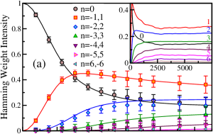
The evolution of the Hamming weights intensities is shown in Fig. 3 (a). The agreement between the experimental data and the numerical simulations for orders up to $n=-6,6$ is excellent. Higher order terms develop at even longer times and are more challenging to detect experimentally. This figure reveals the details of how information lost from the central spin gets shared with the surrounding qubits.

Correlation Rényi Entropies.– We use the Hamming weights intensities $\mathsf{C}^{\mathsf{x}}_{n}(T)^{2}$ to compute the correlation Rényi entropy. The first and second order correlation Rényi entropies are respectively defined as

$$S_{1} = -\sum_{n}\mathsf{C}^{\mathsf{x}}_{n}(T)^{2}\text{log}_{2}\mathsf{C}^{\mathsf{x}}_{n}(T)^{2},$$ (6)

$$S_{2} = -\text{log}_{2}\left(\sum_{n}\mathsf{C}^{\mathsf{x}}_{n}(T)^{4}\right).$$ (7)

They describe the growth of multi-spin correlations in the $x$-axis. Absence of correlations implies that $S_{1}^{\text{min}}=S_{2}^{\text{min}}=0$, while the homogeneous distribution of correlations among all orders, that is $\mathsf{C}^{\mathsf{x}}_{n}(T)^{2}=(2N+1)^{-1}$, leads to the maximum value, $S_{1}^{\text{max}}=S_{2}^{\text{max}}=\text{log}_{2}(2N+1)$.

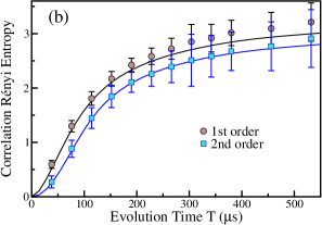
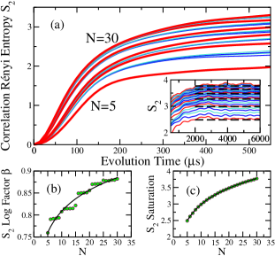
The experimental data for both entropies are compared with numerical simulations in Fig. 3 (b). One sees that the growth of $S_{1,2}$ is not complete during the timescale of our experiment. The correlation Rényi entropy keeps increasing for $T>500\mu$s, implying that the growth of the volume of correlations has not yet ceased and correlations of higher orders are still developing. In fact, as the simulations for different bath sizes in the inset of Fig. 4 (a) indicate, saturation happens at $T\sim 2000\mu$s. This contrasts with the entanglement entropy displayed in Fig. 2 (b), where the curves are already flat for times one order of magnitude shorter, at $T\sim 200\mu$s.

The discrepancy between the timescales for the equilibration of $S_{1,2}$ and $S_{\text{ent}}$ motivated us to have a closer look at the saturation of the entanglement entropy. By significantly zooming in the $y$-axis of Fig. 2 (b), we observe in the inset that $S_{\text{ent}}$ for different bath sizes actually keeps increasing for $T>500\mu$s. It is only because we have a detailed picture of the growth of the volume of correlations, that we could have expected the existence of this residual increase. The evolution of the entanglement entropy, just as the FID, reflects the loss of information from the central spin, as characterized by the decay of $\mathsf{C}^{\mathsf{z}}_{0}(T)$, and this decay happens simultaneously with the growth of the higher order correlations. While the necessary precision to detect the growth of $S_{\text{ent}}$ for $T>200\mu$s is experimentally unreachable, the experimental increase of $S_{1,2}$ at these long timescales is evident in Fig. 3 (b).

Equilibration.– The complete saturation of the correlation Rényi entropy takes place once the clusters of correlated spins stop growing, that is, when the Hamming weights intensities become constant, as seen in the inset of Fig. 3 (a). To estimate the timescale for the equilibration and how it depends on the bath size, we study numerically in Fig. 4 (a) the evolution of $S_{2}$ for baths ranging from $N=5$ to $N=30$.

Figure 4: In (a): Evolution of the correlation Rényi entropy $S_{2}$ for $N=5,\ldots 30$ averaged over 300 orientations of the molecules for $N=5,\ldots 24$ and over 100 or 20 realizations for the largest sizes. The thick red lines correspond to bath sizes that are multiples of 5. The inset in (a) shows the curves up to saturation and $\overline{S_{2}}$ is indicated with dashed lines. In (b): scaling analysis of the factor $\beta$ in $S_{2}(T)\sim-4.18+\beta\log_{2}(T)$ (symbols) fitted with $0.65+0.07\ln(N)$ (solid line). In (c): scaling analysis of the saturation values of $S_{2}$ (symbols) fitted with $1.34+0.71\ln(N)$ (solid line).

We compute the saturation value of the entropy, $\overline{S_{2}}$, by averaging the values of $S_{2}(T)$ for $T>5000\mu$s, when the curves are clearly flat, as seen in the inset of Fig. 4 (a). We then obtain the equilibration times $T_{eq}$ by verifying where each numerical curve of $S_{2}(T)$ first crosses its saturation point. We find that $T_{eq}=(2052.1\pm 163.7)\mu$s for $N=5\ldots 30$, while considering only larger bath sizes, $N\geq 15$, the fluctuations decrease and we get $T_{eq}=(2145.5\pm 39.4)\mu$s.

The fact that $T_{eq}$ is nearly independent of system size is likely a consequence of the fact that both the growth rate of $S_{2}(T)$ and also its saturation value scale as $\ln(N)$. We fit the evolution of $S_{2}$ in the interval $50\mu$s $<T<300\mu$s with the logarithmic function $\alpha+\beta\log_{2}(x)$, where $\alpha$ and $\beta$ are fitting constants. The fitting improves for larger system sizes and we find that the factor $\beta$ increases as $\ln(N)$, as shown in Fig. 4 (b). Since the bath is simulated using rings of 5 spins, similar to the physical sample in Fig. 1, whenever a new ring is introduced, $\beta$ surges with the addition of the first spins, which are closer and thus more strongly coupled with the central spin. As for $\overline{S_{2}}$, the scaling analysis in Fig. 4 (c) demonstrates that it also increases as $\ln(N)$.

Conclusion.– We introduced and experimentally measured the correlation Rényi entropy, which quantifies the volume of multi-spin correlations. The experimental resources needed to measure this entropy in the central spin model scales linearly with the size of the composite system. While the entanglement entropy, $S_{\text{ent}}$, quantifies the loss of information from the central spin, the correlation Rényi entropy, $S_{\text{1,2}}$, provides a more detailed picture of the dynamics of the composite system by capturing how that information gets shared among the bath spins. Most notably, the $S_{\text{1,2}}$ saturates at a time that is an order of magnitude larger than the saturation time for $S_{\text{ent}}$. The correlation Rényi entropy opens interesting perspectives for experimental detection of many-body correlations growth and the spread of quantum information in quantum devices. It may find applications in quantum error correction codes, where information is encoded in long-range quantum many-body states, and in studies of the propagation speed of correlations.