Determining the proton content with a quantum computer

Abstract

We present a first attempt to design a quantum circuit for the determination of the parton content of the proton through the estimation of parton distribution functions (PDFs), in the context of high energy physics (HEP). The growing interest in quantum computing and the recent developments of new algorithms and quantum hardware devices motivates the study of methodologies applied to HEP. In this work we identify architectures of variational quantum circuits suitable for PDFs representation (qPDFs). We show experiments about the deployment of qPDFs on real quantum devices, taking into consideration current experimental limitations. Finally, we perform a global qPDF determination from collider data using quantum computer simulation on classical hardware and we compare the obtained partons and related phenomenological predictions involving hadronic processes to modern PDFs.

I Introduction

Quantum computing is a new computation paradigm that exploits the laws of quantum mechanics to provide new strategies for addressing problems that are nowadays considered to be difficult. The first quantum algorithms showing any advantage over their classical counterparts date from the 1990s, being Shor’s algorithm for integer factorization and Grover’s search the most prominent ones [1, 2]. During the last decade, we have witnessed an impressively fast development of quantum computing, both for theoretical work and hardware implementation perspectives. Nevertheless, currently existing quantum devices are not powerful enough to run competitive quantum algorithms, with respect to the state of the art of the classical ones.

Recent achievements such as quantum supremacy [3] have introduced the so-called Noisy Intermediate-Scale Quantum (NISQ) stage [4]. NISQ devices suffer from errors due to decoherence, noisy gates and erratic read-out measurements, and thus, its performance is limited. However, even at this early stage, quantum technologies may provide useful tools for a broad range of applications. On the one hand, some standard fully determined algorithms are well suited for NISQ processors [5, 6, 7, 8, 9]. In particular, there also exist some examples of quantum algorithms designed to address some problems in high energy physics (HEP) [10, 11, 12, 13]. On the other hand, the approach usually taken to harness the computational power of these imperfect machines is based on hybrid methods combining quantum and classical resources. For example, variational algorithms can be created whose purpose is to optimize some quantity encoding a solution for a specific problem. Among the great variety of quantum variational algorithms it is possible to find examples in quantum chemistry [14, 15, 16, 17, 18], quantum simulation [19, 20, 21], combinatorial optimization [22], solving linear systems of equations [23, 24, 25] and state diagonalization  [26, 27]. Some of these examples are already characterized as Quantum Machine Learning (QML) applications, based on variational [28, 29, 30, 31, 32] and non-variational [33, 34, 35] approaches. Furthermore, QML is a field that is expected to surpass the current performance and ubiquity of classical Machine Learning (ML) when the current limitations of quantum devices will be overcome.

The QML approach to quantum computing is an interesting research topic which can be adapted and tested on research problems already addressed by ML techniques. Motivated by this idea, we propose to investigate the possibility to use quantum computing for the determination of parton distribution functions (PDFs). In perturbative QCD, PDFs are used to describe the non-perturbative structure of hadrons [36, 37]. These functions are typically determined by means of a supervised regression model which compares a wide set of experimental data with theoretical predictions computed with a PDF parametrization.

In this work we first propose the most suitable QML architecture for PDFs representation and then perform experiments about its deployment on real quantum devices, taking into account the current experimental limitations. Then, we adapt the NNPDF methodology [38, 39, 40, 41, 42, 43, 44], based on ML techniques, to operate in a QML environment, replacing Neural-Networks with quantum circuits.

The novel quantum circuit parametrization for PDFs, that we call qPDFs in the next paragraphs, follows the quantum model described in Ref. [28]. The model is constructed as a Parameterized Quantum Circuit (PQC) whose inner parameters depend both on PDF data and trainable parameters. A PQC whose parameters are trainable is known as a Variational Quantum Circuit (VQC). The circuit is applied to an initial quantum state, for instance the ground state $\ket{0}$, and the output state contains information on PDFs. The determination of the circuit parameters is done with standard classical optimization methods, using a predefined cost function.

There are different reasons for attempting a qPDFs determination. First, quantum computing is expected to have a reduced energy consumption when compared to an equivalent classical computer, and thus, we may expect saving power and reducing its environmental impact. Secondly, as we show in this work, the number of parameters needed to obtain an acceptable PDF fit is in average lower with quantum models in comparison to modern PDF models. Furthermore, the qPDF approach may take advantage from quantum entanglement, since the potential outstanding power of quantum computing emerges from there. Finally, quantum hardware may bring performance improvements in terms of running time for this model when compared to the standard ML approach since the number of operations needed to obtain an acceptable solution is lower and the model has an exact hardware representation. On the other hand, we consider the qPDF model presented in this work as proof-of-concept for future implementations, given that the performance of quantum simulation on classical hardware and the stability of real quantum device measurements are not competitive with the ML tools used by modern PDF determinations.

The paper is structured as follows. Sec. II provides an overall description of the quantum circuit model for PDFs, while in Sec. III we identify its best architecture. In Sec. IV we discuss about the deployment of qPDFs on real quantum devices. In Sec. V we integrate the qPDF model in the NNPDF fitting framework and perform a first global qPDF determination using data from experiments such as Tevatron or LHC. In Sec. VI we compute Higgs observable predictions using the qPDF fit. Finally, in Sec. VII we present our conclusion and future development directions.

II Quantum circuits for PDFs

Quantum circuits are mathematically defined as operations acting on an initial quantum state. Quantum computing usually makes use of quantum states constructed out of qubits, that is, binary states represented as $\ket{\psi}=\alpha\ket{0}+\beta\ket{1}$. The states of a quantum circuit are commonly defined by its number of qubits $n$, and, in general, the initial state of the circuit $\ket{\psi_{0}}$ is the zero state $\ket{0}^{\otimes n}$. A quantum circuit implements an inner unitary operation $\mathcal{U}$ to the initial state $\ket{\psi_{0}}$ to transform it into the final output state $\ket{\psi_{f}}$. For some algorithms, this $\mathcal{U}$ gate is fully determined [1, 2], while other algorithms define its inner operation by means of some fixed structure, so-called Ansatz, and tunable parameters $\mathcal{U}(\theta)$ [14, 23, 24]. Those are known as Parameterized Quantum Circuits (PQC). This kind of circuits is useful in the NISQ era of quantum computing, since they provide a great flexibility and allow to approximate unitary operations up to arbitrary precision [45, 46]. The parameters defining the PQCs can be trained using an optimization procedure known as a Variational Quantum Circuit (VQC). It is possible then to use classical computational resources to find the optimal configuration of a quantum circuit.

A VQC follows roughly three steps to solve a given problem, as schematically shown in Fig. 1. First, a PQC $\mathcal{U}(\theta)$ is constructed using a small set of single- and two-qubit parametric gates. The Ansatz of such circuit may follow a particular path exploiting the special features of the problem, or may also be a general one. After the Ansatz is applied to the circuit, we must perform some measurements on the output quantum state to extract information. Those measurements are used to evaluate a loss function $\mathcal{L}(\theta)$ encoding the problem. The loss function should reach its minimum as the problem is perfectly solved. The loss function $\mathcal{L}(\theta)$ is passed to a classical optimizer that looks for the value

$$\theta^{*}={\rm argmin}\left(\mathcal{L}(\theta)\right).$$ (1)

Classical optimizers need several function evaluations, thus when modifying the set of parameters $\theta$ the Ansatz $\mathcal{U}(\theta)$ is updated and new measurements are performed. Although the general scheme for variational circuits is pretty simple, lots of details can be deployed regarding the three pieces of this algorithm.

$$\Qcircuit@R=0.5em@C=0.3em{\lstick{\ket{0}}&\qw\multigate{2}{\mathcal{U}(\theta)}\qw\meter\cw\control\cw\\ \lstick{\ket{0}}\qw\ghost{\mathcal{U}(\theta)}\qw\meter\cw\control\cwx\cw\push{\Downarrow}\\ \lstick{\ket{0}}\qw\ghost{\mathcal{U}(\theta)}\qw\meter\cw\control\cwx\cw\\ \Uparrow\control\cwx\gate{\rm Classical\,Optimizer}\cw\dstick{\Leftarrow}\cw\gate{\mathcal{L}(\theta)}\cw\control\cwx\cw\\ }$$

Figure 1: Operational scheme of a Variational Quantum Circuit. A unitary gate $\mathcal{U}$, depending on some parameters $\theta$, transforms the initial $\ket{0}$ state into some output state. This state is measured and used to compute a loss function $\mathcal{L}(\theta)$. The classical optimizer performs an update on the parameters to minimize the value of $\mathcal{L}(\theta)$. New parameters are then sent to the quantum circuit and the loop starts again.

We propose a model based on the general framework of VQC to tackle the problem of fitting one or several PDFs flavours using quantum computers. In this case, the problem to be solved is mathematically reduced to approximate arbitrary one-dimensional functions within a certain target accuracy. That is, we define the PDF model to be parametrized by a VQC as

$${\rm qPDF}_{i}(x,Q_{0},\theta),$$ (2)

where $x$ is the momentum fraction of the incoming hadron carried by the given parton with flavour $i$ (quarks and gluon), so $0\leq x\leq 1$, at a fixed initial energy scale $Q_{0}$. Following this definition, we propose some superficial modifications to adjust the VQC to this particular problem.

First, we need to introduce the value of $x$ into the circuit. Thus, we modify the definition of the Ansatz to depend on $\theta$ and $x$, that is $\mathcal{U}(\theta)\rightarrow\mathcal{U}(\theta,x)$. This $x$ value is introduced as inner circuit parameters following the re-uploading procedure in Ref. [28]. The effect of the quantum circuit is then defined as

$$\mathcal{U}(\theta,x)\ket{0}^{\otimes n}=\ket{\psi(\theta,x)},$$ (3)

which produces a significant change in the output state, since it depends now on $x$ and not only on $\theta$. The key ingredient in this approach is that, as the variable $x$ serves as input several times in every circuit, it is possible to obtain non-linear mathematical structures that allow arbitrary fittings. The exact design of some $\mathcal{U}(\theta,x)$ Ansätze are further explained in Sec. III.2.

The second ingredient in our model is the way PDF information is extracted from the quantum circuit. We use the $Z$ Pauli gates to define a series of Hamiltonians to perform measurements with. Let us consider a $n$-qubit circuit to run our variational algorithm on. The set of Hamiltonians to build is

$$Z_{i}=\bigotimes_{j=0}^{n}Z^{\delta_{ij}},$$ (4)

where $\delta_{ij}$ is the Kronecker delta function.

The choice of this Hamiltonian is heuristic. This model creates as many Hamiltonians as qubits are available in the circuit, and those Hamiltonians are created by measuring a certain qubit with the $Z$ Pauli matrix, while all other qubits remain unmeasured. These observables measures the population of the states $\ket{0}$ and $\ket{1}$ of a particular qubit. The hamiltonian is proposed in order to encode the PDF functions within the probability of measuring a certain qubit in its excited state. Following the Hamiltonians previously stated, we can define the function

$$z_{i}(\theta,x)=\bra{\psi(\theta,x)}Z_{i}\ket{\psi(\theta,x)}.$$ (5)

The next step is to relate these $z_{i}$ functions to the PDF values. We associate each function $z_{i}(\theta,x)$ to only one parton $i$. That is, if the model aims to fit $n$ partons, the circuit width must be $n$ qubits. We define the qPDF model for flavour $i$ at a given $(x,Q_{0})$ as

$${\rm qPDF}_{i}(x,Q_{0},\theta)=\frac{1-z_{i}(\theta,x)}{1+z_{i}(\theta,x)}.$$ (6)

With this choice only positive values are available, although there is no upper bound. The reason to choose this particular definition is heuristic and is supported by empirical results detailed in a later section. It is, however, not a hard constraint, as it is possible to drop this positivity constraint with a simple re-scaling. A theoretical motivation can be drawn from the fact that PDF functions can be made non-negative [47] but their values may in principle grow to any real value, see for instance the gluon PDF in Fig. 4.

III Implementation

III.1 Workflow design

Figure 2: Schematic workflow for the implementation of qPDF.

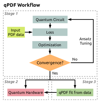
In order to achieve our goal to determine a set of PDFs based on quantum circuits, we have defined a workflow based on a step-by-step procedure composed by three stages: (1) the identification of the most adapted quantum circuit Ansatz for qPDF parametrization, (2) the feasibility study to deploy the qPDF model into real quantum devices, and finally, (3) the integration of the quantum circuit model in a global PDF fitting framework.

In Fig. 2 we show schematically the three stages we followed. Firstly, we perform simulations to identify the best model architecture and capacity to represent PDF-like functions. This stage is similar to the usual hyper-optimization tune performed in Machine Learning applications. However, in our context, we do not have a specific initial Ansatz assumption, thus empirical tests and fine-tune is required. These simulations are done by computing the exact wave-function of all quantum states involved in the middle steps of the algorithm using classical hardware. The expected values for Hamiltonians are also exactly computed and not measured. The model is then trained to fit PDF input data generated from the NNPDF3.1 set of PDFs [42]. In the next section we discuss the details of the procedure and identify the best model architecture for the qPDF determination.

The second stage studies the possibility to deploy the qPDF model in an actual quantum device. For this step, we introduce measurements and noise models, and identify the required number of shots and trials for an acceptable representation of PDFs.

Finally, as a third and last stage, we use this model in an actual PDF fit based on experimental data (mainly comprised of LHC measurements). We have integrated the qPDF model from stage 1 in the NNPDF fitting framework [38, 37]. This implementation opens the possibility to perform fits on the same datasets of modern PDF releases.

All calculations involving quantum circuits are performed using the quantum simulation tool Qibo [48, 49] on classical hardware. The qPDF model is publicly available through the Qibo API. The experimental implementation of this model was done using Qiskit [50] from the OpenQASM [51] code generated by Qibo. The processing of experimental data from the LHC experiments is done with the n3fit [38] code.

III.2 Ansatz determination

@R=.75em @C=.4em & 7U^l(θ_l, γ_l, x)           U(θ_l,0, x) 1 R_z(γ_l,7)
U^l(θ_l, γ_l, x)           U(θ_l,1, x) R_z(γ_l,0) 1
U^l(θ_l, γ_l, x)           U(θ_l,2, x) 1 R_z(γ_l,4)
U^l(θ_l, γ_l, x)           U(θ_l,3, x) R_z(γ_l,1) 1
U^l(θ_l, γ_l, x) =     U(θ_l,4, x) 1 R_z(γ_l,5)
U^l(θ_l, γ_l, x)           U(θ_l,5, x) R_z(γ_l,2) 1
U^l(θ_l, γ_l, x)           U(θ_l,6, x) 1 R_z(γ_l,6)
U^l(θ_l, γ_l, x)           U(θ_l,7, x) R_z(γ_l,3) -7

(a)     One layer

@R=.46em @C=.4em & 7U(x, θ, γ)           7U^0 ⋯ 7U^l ⋯ U^L-1_0
U(x, θ, γ)           U^0 ⋯ U^l ⋯ U^L-1_1
U(x, θ, γ)           U^0 ⋯ U^l ⋯ U^L-1_2
U(x, θ, γ)           U^0 ⋯ U^l ⋯ U^L-1_3
U(x, θ, γ) =     U^0 ⋯ U^l ⋯ U^L-1_4
U(x, θ, γ)           U^0 ⋯ U^l ⋯ U^L-1_5
U(x, θ, γ)           U^0 ⋯ U^l ⋯ U^L-1_6
U(x, θ, γ)           U^0 ⋯ U^l ⋯ U^L-1_7

(b)     Full Ansatz

Figure 3: On the left we show an example of one layer architecture. On the right we present the scheme of a full Ansatz circuit including 8 qubits and entangling gates. The $U^{l}(\theta_{l},\gamma_{l},x)$ from the left figure enters the full ansatz as $U^{l}$. Note that the last layer does not have any entangling gate.

We discuss now the different Ansätze that are considered in this work. Two main different kinds of Ansätze were designed. The first one, named Weighted Ansatz, is directly inherited from Ref. [28], and introduces the $x$ variable using the weights and biases scheme, similarly to Neural Networks. The second one, called Fourier Ansatz, inspired in Ref. [52], is related to harmonic analysis and uses linear and logarithmic scaling to satisfy all values of $x$ involved in PDF determination, in particular for small and large values of $x$, where experimental data suffers from larger uncertainties. The main difference between both Ansätze is the presence or absence of tunable weights.

In the Weighted case, the single-qubit gate serving as building block for the whole Ansatz is

$$U_{w}(\alpha,x)=R_{z}(\alpha_{3}\log(x)+\alpha_{4})R_{y}(\alpha_{1}x+\alpha_{2}),$$ (7)

where $\alpha$ is a four-component set of parameters. Notice that two different axis are involved in the definition of this gate. This is due to the fact that any two different Pauli matrices do not commute and leads to the rising of non-linear mathematical structures, allowing the approximation to be uniformly accurate [28, 53, 54]. The presence of both axis allows the possibility to introduce $x$ and $\log(x)$ dependencies to the same gate.

In the Fourier case, we define the gate

$$U_{f}(\alpha,x)=R_{y}(\alpha_{4})R_{z}(\alpha_{3})R_{y}(-\pi/2\log x)\\ R_{y}(\alpha_{2})R_{z}(\alpha_{1})R_{y}(\pi x)$$ (8)

where the values of the coefficients preceding the $x$ and $\log(x)$ depend on our dataset. For the specific PDF determination problem presented here, the values of $x$ are constrained to lie between $10^{-4}$ and $1$, thus the gates are evaluated at angles between $0$ and $2\pi$.

We use these single-qubit gates to construct layered Ansätze to fit the PDFs. The reason for this procedure is that we expect to cast more accurately the output quantum state as more layers are added to the quantum circuit. The layers have two pieces. First, a layer of as many single-qubit parallel gates as qubits is applied. Second, a set of entangling gates is added to the circuit. All entangling gates are controlled $R_{z}(\gamma)$ gates, where $\gamma$ is also a tunable parameter. Entangling gates connect one qubit with the next one and then with the previous one, or viceversa. All layers include the entangling pieces except for the last one. A scheme depicting the structure of such this circuit can be viewed in Fig. 3. The parameters entering in every gate are independent for all the other parameters, and all of them are to be optimized simultaneously. Note that single-qubit circuits cannot have any entanglement by definition.

For this first tuning stage, we drop the circuit layer with measurement gates and use simulated final states. The optimization procedure then uses the Pearson’s $\chi^{2}$ loss function [55] to compare the qPDF predictions to the target central values $f_{i}$ of NNPDF3.1 NNLO [42]. In this exercise we always consider a grid of $x$-points distributed between $[10^{-4},1]$ at $Q_{0}=1.65$ GeV and a maximum of 8 flavours for quarks, antiquarks and the gluon: $i\in\{\bar{s},\bar{u},\bar{d},g,d,u,s,c(\bar{c})\}$. The $\chi^{2}$ covariance matrix is set to a diagonal matrix containing the $\sigma_{f_{i}}(x,Q_{0})$ uncertainty of the target set.

Single-flavour fit		Multi-flavour fit
Layers (Parameters)	$\chi^{2}$	$\chi^{2}$	Layers (Parameters)
1 (32)	28.6328		1 (32)
2 (64)	1.0234	–	–
3 (96)	0.0388	0.1500	2 (72)
4 (128)	0.0212	0.0320	3 (112)
5 (160)	0.0158	0.0194	4 (152)
6 (192)	0.0155	0.0154	5 (192)

Table 1: Comparison of $\chi^{2}$ values for the Weighted Ansatz model between the average of all single-flavour fits (left) and the corresponding multi-flavour fit (right).

Single-flavour fit		Multi-flavour fit
Layers (Parameters)	$\chi^{2}$	$\chi^{2}$	Layers (Parameters)
1 (32)	900.694		1 (32)
2 (64)	57.2672	–	–
3 (96)	0.0410	47.4841	2 (72)
4 (128)	0.0232	0.0371	3 (112)
5 (160)	0.0165	0.0216	4 (152)
6 (192)	0.0156	0.0160	5 (192)

Table 2: Comparison of $\chi^{2}$ values for the Fourier Ansatz model between the average of all single-flavour fits (left) and the corresponding multi-flavour fit (right).

Figure 4: Multi-flavour qPDF fits using the Weighted Ansatz (orange curves) and the Fourier Ansatz (blue curves) with 5 layers and 8 qubits. The mean value and $1\sigma$ uncertainty of the target PDF data is shown by means of a solid black line and a shaded grey area.

Figure 5: Comparison between single-flavour fits (left) and multi-flavour fits (right) for the gluon, up and strange quarks PDFs. For the single-flavour fits the Weighted Ansatz (orange curves) and Fourier Ansatz (blue curves) are composed by 1 qubits and 6 layers. On the other hand for the multi-flavour fits, the Ansätze are composed by 8 qubits and 5 layers. The mean value and $1\sigma$ uncertainty of the target PDF data is shown by means of a solid black line and a shaded grey area.

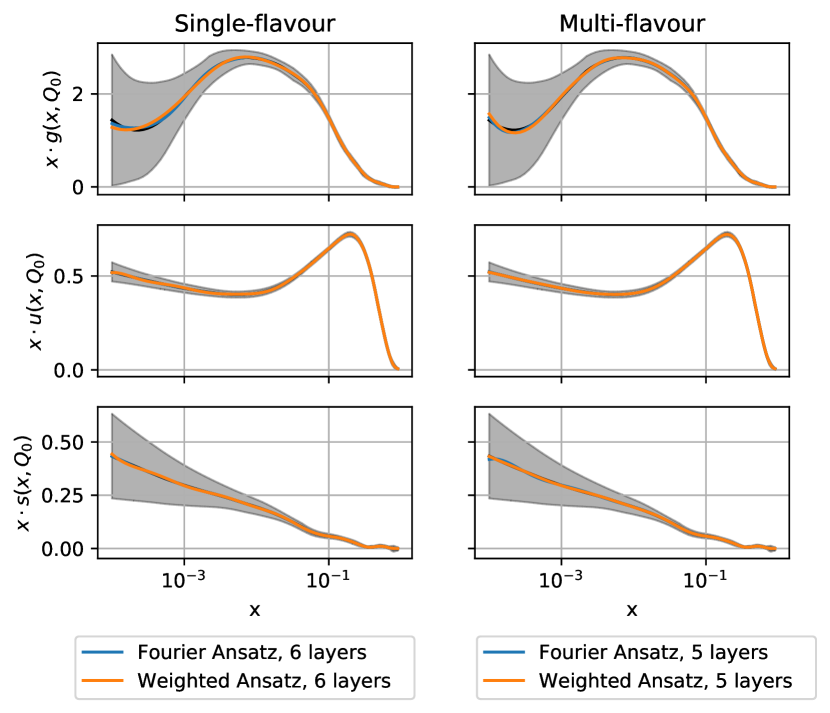
Results summarized in Tables 2 and 2 show the values for Pearson’s $\chi^{2}$ function both for the Weighted and the Fourier Ansätze respectively. In both cases, the left column shows an average fit for all the flavours in a one-by-one fashion, while the right column shows an optimization for all flavours simultaneously. These table compare the performance between circuits with similar number of parameters, that is, in every pair unentangled circuits have a larger number of layers than entangled circuits. The reason to compare circuits in this way is because entanglement is expected to improve the overall quality of the fits. The calculations were in this case made by simulating all the operations on quantum circuits, and the optimization procedure was done in two steps. First, the CMA genetic algorithm is used to find optimal solutions for single-flavour optimizations [56]. In the multi-flavour scenario we used the L-BFGS-B function from scipy [57, 58]. The multi-flavour optimizations start from the corresponding single-flavour results and add the entangling gates, allowing for a better fitting. In addition, some results for the final fitting are to be viewed in Figs. 4 and 5.

There are several interpretations that can be claimed from those results. First, it is clear that entanglement does not suffice to obtain good approximations. Entanglement can be understood as a quantum resource to extract the correlations between different qubits, which in this case encode the information of qPDFs within. On the other hand, every layer of variational gates provides a new step in non-linearity, which is necessary to represent arbitrary functions. Thus, entanglement may help to achieve better fittings, as seen in Tables 2 and 2 for models with the same number of layers. However, a sufficient number of layers is also mandatory. Secondly, data unveils the goodness of the Weighted Ansatz with respect to the Fourier one. Built-in weights grant the model a great representability, especially in the cases with a small number of layers.

As final Ansatz, we will retain the Weighted one with 5 layers both in the single-flavour and multi-flavour scenarios. For the sake of comparison, equivalent Fourier Ansätze are chosen. In the remainder of this work, we are using the 5-layers multi-flavour Weighted Ansatz. This circuit has got 5 layers of single-qubit gates and 4 layers of entangling gates interspersed with the single qubit layers, up to a total amount of 192 parameters, which is a manageable number. A detailed comparison in the number of parameters is deployed in Tab. 3. The entangling gates are controlled-$R_{z}$ gates with one inner parameters, and single-qubit gates are parameterized through the scheme $wx+b$, where $x$ is the variable for the PDFs. Logarithmic and linear scales are used together in the same quantum gate. This configuration is also the first one allowing for a path between all qubits of the circuit. Results depicted in Table 2 and Figs. 4 endorse the use of this Ansatz. In addition, tests run on both Ansätze reveiled that the Weighted Ansatz is easier to train using efficient gradient-based methods such as L-BFGS-B.

	Single-flavour		Multi-flavour
	Weighted	Fourier	Weighted	Fourier
Qubits $(q)$	1 (per flavour)		8
Layers $(l)$	5		5
Parameters	$2\cdot l\cdot q$ weights	$4\cdot l\cdot q$	$16\cdot l$ weights	$32\cdot l$
	$2\cdot l\cdot q$ biases		$16\cdot l$ biases
	No entanglement		$8(l-1)$ entangling

Table 3: Summary for the Ansätze chosen for this work. The preferred number of l ayers was chosen as a compromise between small $\chi^{2}$ and number of parameters. Results depicted in Tables 2 and 2 determine that the multi-flavour Weighted Ansatz is our best candidate model.

IV Experimental configuration

The previous section showed that a low-depth variational Ansatz is capable of expressing the full set of PDF functions, this section investigates how well that expressibility transfers to a realistic quantum computer. In order to understand the effects of noise on the model, the trained single-flavour model was compiled on the IBM Athens quantum processor [50]. In the single-flavour model, each qubit/parton is fit independently of the others, and therefore the circuit can be efficiently represented as a rotation of the Bloch sphere. This fact makes the single-flavour model robust to single-qubit gate errors. Each parton was evaluated at 20 logarithmically-spaced points between $10^{-4}<x<1$. At each point, the expectation value, $z_{i}=\langle\psi|Z_{i}|\psi\rangle$, is estimated using $8192$ shots. The evaluation of each point was repeated five times in order to probe the statistical uncertainty in estimation, it was found that the estimation was robust to statistical noise. Fig. 6 shows the comparison of running the experiment, and the simulation results. From this figure we deduce that the single-flavour model produces acceptable results on currently available quantum computers, and that the Qiskit noise simulation environment does a good job of predicting the outcome of the experiment.

Figure 6: Single-flavour fit for all flavours, using the Weighted Ansatz, for 5 layers and 8 qubits, that is one qubit per flavour. The red lines represent the prediction of the qPDF model with simulated noise from the IBM Athens processor [50]. Green points are the results of running the circuit on the Athens quantum processor. The mean value and $1\sigma$ uncertainty of the target PDF data is shown by means of a solid black line and a shaded grey area.

In order to gain an understanding of how the proposed multi-flavour model performs on a quantum computer, the optimized circuit was simulated with a realistic noise model. The first step of this simulation is to explicitly include the measurement gates in the circuit as can be seen in Fig. 3. Each qubit represents a particular parton, and therefore the qubits should be measured independently. The goal of the measurement is to estimate $z_{i}=\langle\psi|Z_{i}|\psi\rangle$, this is achieved in a given number of shots by subtracting the number of occurrences of measuring 1 from the number of occurrences of measuring 0, and normalizing by number of shots.

The ability of the circuit to reproduce the PDF was first simulated on an ideal quantum computer using Qiskit [50]. The simulation was performed with $8192$ shots as this value corresponds to the maximum number of shots permitted per run on IBM quantum processor. It was found that this number of shots was more than sufficient to converge the estimate of $\langle\psi|Z|\psi\rangle$, and thus accurately reconstruct the PDF. This is shown in Fig. 7.

Figure 7: Multi-flavour fit for all flavours, using the Weighted Ansatz, for 5 layers and 8 qubits, that is one qubit per flavour. Blue lines are the mean and the blue shadowed area the $1\sigma$ uncertainty of the circuit measurement results for an ideal noise free quantum device. The red curve refers to simulated circuit measurements using the noise model for the IBM Melbourne processor [50]. Similarly, green and orange curves show simulation results with noise reduced by 50% and 90% respectively. The mean value and $1\sigma$ uncertainty of the target PDF data is shown by means of a solid black line and a shaded grey area.

In order to simulate the effect of a realistic noise model, the IBM Melbourne quantum processor was chosen [50]. The Melbourne processor is the only device that is publicly available through the IBM Quantum Experience that has enough qubits to fit the optimized circuit. The 8 qubit optimized circuit was mapped onto Melbourne in such a way to minimize the $\chi^{2}$.

The errors on the Melbourne device were found to drastically deteriorate the estimation of the PDF as can be seen in Fig. 7. This analysis has shown that while it is possible in theory to fit a PDF using a quantum computer, the noise in the current state-of-the-art quantum processors is still too high to reconstruct the PDF accurately.

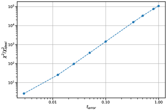
Another question that can be asked is, how robust must the quantum device be in order to have an acceptable representation of the PDF? To answer this question, a simplified version of the Melbourne device was created. In this simplified Melbourne, all the qubits and connections were taken to have identical noise characteristics, specifically all single gate, double gate, and readout errors were set to the best values from the real Melbourne processor. With this simplified device, the noise models can be uniformly scaled down to interpolate between an ideal quantum computer and a Melbourne-like device using a parameter $t_{\text{error}}$, where $t_{\text{error}}=0$ corresponds to an ideal quantum computer, and $t_{\text{error}}=1$ corresponds to the simplified Melbourne device. Fig. 8 shows what happens to the cost function $\chi^{2}$ as $t_{\text{error}}$ is varied.

Figure 8: The error as a function of the error interpolation parameter $t_{\text{error}}$. The $y$-axis is given as the ratio between the error, $\chi^{2}$, and the error on an ideal quantum computer, $\chi_{\text{ideal}}^{2}$.

V PDF determination from experimental data

In the previous sections we have described the process of finding a final Ansatz which can encode the full complexity of the physical PDFs by training to already known results. Furthermore, we have verified the possibility to deploy such model on real quantum devices. These steps correspond with stages 1 and 2 of our workflow (Fig. 2) where the PDF is treated as a known quantity. In reality, however, the only data that one has access to are the experimental measurements of physical observables performed at experiments (for instance, physical cross sections measured at the LHC).

The next stage of this work is to prove that this methodology can also replace the neural networks at the core of the NNPDF methodology for fitting PDFs. Although still far from being of practical usaged (see for instance Fig. 4) we show, in the simulator, that a hybrid VQE could indeed replace neural networks as an universal function approximator for complex problems such as the one posed by parton distribution functions.

In this final section we start by describing the NNPDF methodology and what changes are needed to its latest implementation (described in [38]) to perform a full fit. We use the NNPDF3.1 dataset which includes deep-inelastic scattering (DIS) and hadronic collider data. We end with a comparison between our resulting PDF (qPDF) and the latest NNPDF release (NNPDF3.1) and prove that the results are perfectly usable in an actual computation of physical observables.

V.1 The NNPDF fitting methodology

The two main aspect that define the NNPDF methodology are the Monte Carlo approach to the uncertainties of experimental measurements and the usage of Neural Networks (hence the name) to model the PDFs. In this section we outline some of the most relevant aspects of the NNPDF methodology, for a more in-depth review please consult [43].

The first step of the methodology is the generation of “data replicas”. This procedure propagates the experimental uncertainties into the PDF fit by leveraging the covariance matrices provided by the experiments by creating between 100 and 1000 artificial copies of the data as if they were produced by independent measurements.

The full PDF fitted in this methodology follows the functional form for each parton $i$:

$$f_{i}(x,Q_{0})=x^{-\alpha_{i}}(1-x)^{\beta_{i}}{\rm NN}_{i}(x),$$ (9)

where the fitted NN is prepended by a preprocessing factor per parton $x^{-\alpha}(1-x)^{\beta}$. This factor ensures the correct behaviour at very small (close to 0) and very large (close to 1) values of $x$, where there might not be enough experimental data to properly constraint the NN. This function constrains all free parameters that define the behaviour of the PDF. The functions defined in Eq. (9) however cannot be directly compared to experimental data, instead one would have to convolute them with the partonic cross section in order to obtain a physical prediction that can be compared to the result of an experiment,

$$P=\displaystyle\int\differential{x_{1}}\differential{x_{2}}f^{i}_{1}(x_{1},q^{2})f^{j}_{2}(x_{2},q^{2})|M_{ij}(\{p_{n}\})|^{2},$$ (10)

where $x_{1},x_{2}$ are the momentum fraction carried by the two colliding partons and the indices $i$ and $j$ run over all possible partons. $M_{ij}$ is the matrix element for the given processes and $\{p_{n}\}$ represents the phase space for a $n$-particles final state. Performing this integral numerically per training step, per experimental data point, would be completely impracticable. Instead the theoretical predictions are approximated as a product between the PDF model and a fastkernel table (FK table) encoding all the relevant information on the computation as described in Refs. [59, 60].

The optimization of the function defined in Eq. (9) consists then in the minimization of a $\chi^{2}$ defined as:

$$\chi^{2}=\sum_{i,j}^{N_{\rm dat}}(D-P)_{i}\sigma_{ij}^{-1}(D-P)_{j},$$ (11)

where $D_{i}$ and $P_{i}$ are respectively the $i$-nth data point from the training set and its theoretical prediction and $\sigma_{ij}$ is the experimental covariance matrix provided by the experimental collaborations.

This procedure is then repeated for each of the artificial replicas. Note that the theoretical predictions are always the same, so the only change between replicas is in the experimental data points. The final central value for the PDF is then the average over all replicas, while the error bands are given by taking the envelope that contains 68% of all replicas.

V.2 Qibo-based n3fit

The latest implementation of the latest iteration of the NNPDF methodology is described in Ref. [38]. This implementation is very modular and one can seamlessly swap the Tensorflow based backend by any other provider. Qibo, which is also partially based on Tensorflow can be easily integrated with the NNPDF methodology.

Note that all results in this section corresponds to the simulation of the quantum device on classical hardware. Such a simulation is very costly from a computational point of view which introduces a number of limitations that need to be addressed in order to produce results in reasonable time frames.

FK reduction: the definition of the quantum circuit depends on both the set of parameters $\theta$ and the value of the parton momentum fraction $x$ (see Eq. (3)) which means the circuits needs to be simulated once per value of $x$. The union of all FK tables for all physical observables (following Eq. (10)) amounts to several thousand values of $x$. Since such a large number of evaluations of the quantum circuit is impracticable, we introduce a further approximation where each partial FK table is mapped to a fixed set of 200 nodes in the x-grid. This simplification introduces an error to the total $\chi^{2}$ of the order of $\Delta\chi^{2}=0.14\pm 0.01$ when averaged over PDF members. This error on the cost function is however negligible for the accuracy reached in this work.

Positivity: in the fitting basis, as defined in section II, the PDF cannot go negative. Physical predictions however are computed in the flavour basis [61] where the rotation between basis can make some results go negative. However, physical observables (differential or total cross sections) cannot be. This physical constraint is included in NNPDF3.1 via fake pathological datasets. These have not been implemented for qPDF as they correspond to a fine-tuning of the methodology which is beyond the scope of this work.

Figure 9: Predictions for a toy $s\bar{s}$ initiated Drell-Yan process with qPDF and a simplified version of NNPDF3.1 where the positivity constraint has been removed.

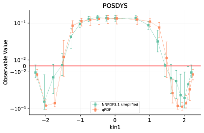
The removal of the positivity constraint from the fit introduces an unphysical distortion to the results as the PDF could produce negative predictions for physical predictions. Such results are unphysical because they would correspond to situations in which the probability of finding a particular phase space configuration is negative, which makes no sense. In Fig. 9 we compare the “negativity” between qPDF and a version of NNPDF3.1 with the positivity constraints removed. We observe that both fits behave similarly, proving such unphysical results are a consequence of the removal of the constraint rather than a problem in the qPDF methodology.

Momentum Sum Rule: the PDFs as defined in Eq. 9 are normalized such that [43],

$$\frac{\displaystyle\int_{0}^{1}dx\;x\,f_{g}(x,Q_{0})}{1-\displaystyle\int_{0}^{1}dxxf_{\Sigma}(x,Q_{0})}\simeq 1,$$ (12)

this equation is known as the momentum sum rule and it is imposed in n3fit through an integration over the whole range of x which is impracticable in this implementation for the reasons mentioned above. Instead, in qPDF these are only checked afterwards, finding a good agreement with the expected values (despite not being imposed at fitting time). Indeed, for qPDF the result for the average over all replicas is:

$$\frac{\displaystyle\int_{0}^{1}dx\;x\,f_{g}(x,Q_{0})}{1-\displaystyle\int_{0}^{1}dxxf_{\Sigma}(x,Q_{0})}=1.01\pm 0.01.$$ (13)

which is to be compared with the NNPDF3.1 result of $1.000\pm 0.001$, where the constraint was imposed at fit time.

V.3 qPDF

Once all ingredients are implemented, we are in a position to be able to run a NNPDF3.1-like fit using the new prescription based on the VQE and the Qibo library. As a base reference for the comparison we take the NNPDF3.1 NNLO fit [42], which is the latest release by the NNPDF collaboration. The plots comparing the NNPDF sets with qPDF are then produced using a reportengine [62] based internal NNPDF tool.

The dataset included in this fit correspond to that of NNPDF3.1, which is detailed in Section 2.1 of [42] and includes data from deep-inelastic scattering experiments, fixed-target Drell-Yan-like data and hadronic collider data from experiments at Tevatron and LHC.

Figure 10: $\chi^{2}/N$ per experiment grouping. There is a deterioration of the goodness of the fit (measured by the $\chi^{2}$) for some of the experiments for the central value. The goodness of the fit is very similar between the reference and qPDF for most of the experiments being considered.

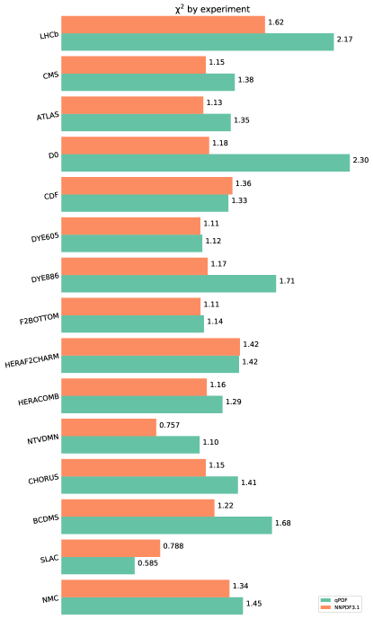
We can start by comparing the $\chi^{2}/N$ result for the datasets that have been considered in the fit, shown in Fig. 10. One would expect a perfect fit when $\chi^{2}/N=1$, however this is not the case even in the reference and it is due to a combination of missing higher order corrections (a lack of a better theory) or inconsistencies in the experimental results,

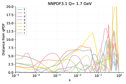
The similarity on the phenomenological results obtained by both fitting methodologies as shown in Fig. 10 is well understood as well by looking at the distance plots between the qPDF and the reference in Fig. 11,

$$d^{2}(f_{i},r_{i})=\frac{\langle f_{i}\rangle-\langle r_{i}\rangle}{\frac{1}{N_{f}}\sigma(f_{i})^{2}+\frac{1}{N_{r}}\sigma(r_{i})^{2}},$$ (14)

where $i$ is the flavour being considered and $f$ and $r$ corresponds to qPDF and the reference (NNPDF3.1) respectively. The central value is taken over the $N$ replicas of the set, generally of the order of 100.

Indeed, for most partons the difference between both fits are under the 1-$\sigma$ level (distance equal to 10 for 100 replicas) growing up to 2-$\sigma$ for the $u$ and $s$ quarks.

Figure 11: Distance (as defined by Eq. (14)) between qPDF and NNPDF3.1. When the distance is kept under $d(f_{i},r_{i})=10$ the two fits are 1-$\sigma$ compatible. All partons except for $u$ and $s$ are below or around the 1-$\sigma$ distance for the entire range considered. Note however, by comparing to Fig. 4 that the fits for both the $u$ and $s$ quarks are compatible in the most relevant regions for these particles.

(a)  Gluon pdf.

(b)  u quark pdf.

(c)  s quark pdf.

Figure 12: Fit results for the gluon and the $u$ and $s$ quarks. As previously seen in Fig. 4, qPDF is able to reproduce the features of NNPDF3.1. We now see this is also true when the fit performed by comparing to data and not by comparing directly to the goal function. The differences seen at low-x can be attributed to the lack of data in that region.

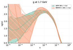
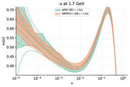
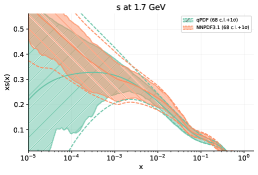
This point is clearly seen in Fig. 12 where we compare the published PDFs (with their corresponding error bars) for the gluon and the $d$ and $u$ quarks. We note that for these quark flavours the qPDF central result is almost always within the 1-$\sigma$ range of the reference, with an overlapping error band for the whole considered range.

(a)  Atlas jets data differential in rapidity [63].

(b)  CMS Z differential in rapidity for fixed value of $p_{T}$ [64].

(c)  LHCb, Z cross section differential in rapidity [65].

Figure 13: Theoretical predictions computed with the method describe in [60] in order to compare the same prediction with three different PDF sets. We note that the predictions for the qPDF set is compatible with both the experimental measurements and the released PDF set. The parton-level calculation has been performed with the NLOjet++ [66] and MCFM [67] tools.

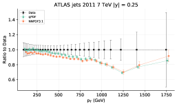
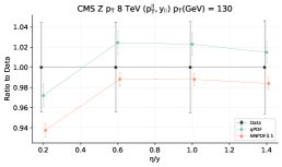
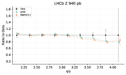
In Fig. 13 we show specifically a comparison between the reference NNPDF3.1 and qPDF for selected datasets, we also provide the LHAPDF-compatible PDF grid. We observe that the accuracy of the qPDF central value is similar to that of NNPDF3.1. Furthermore, the error bars for the predictions of both PDF set overlap with the experimental error bars, and, in some cases, also among themselves.

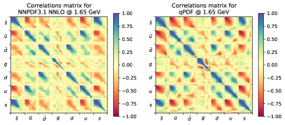
Finally, in Fig. 14 we compute the PDF correlations for NNPDF3.1 and qPDF replicas using Pearson’s coefficient in a fixed grid of 100 points distributed logarithmically in $x=[10^{-4},1]$.

This leads us to conclude that the methodology described in this paper can be used for regression problems to unknown functional forms such as the proton internal structure and produce results that are perfectly coherent, from a phenomenological point of view, with the state of the art. In addition we believe that with adequate tuning one could achieve the same level of accuracy of the classical approach.

We finalize this section by showing phenomenological results where the LHAPDF grids produced with this approach are used for a full fixed order prediction. In summary going back circle to the master equation, i.e., computing numerically Eq. (10) with no approximations using state of the art tools.

Figure 14: PDF correlation matrix for flavours in a grid of $x$ points for NNPDF3.1 NNLO (left) and the qPDF (right).

VI Phenomenological results

Channel	NNPDF3.1 NNLO	qPDF
$ggH$	$31.04\pm 0.30$ pb	$31.71\pm 0.51$ pb
$t\bar{t}H$	$0.446\pm 0.003$ pb	$0.464\pm 0.008$ pb
$WH$	$0.133\pm 0.002$ pb	$0.135\pm 0.002$ pb
$ZH$	$0.0181\pm 0.0002$ pb	$0.0184\pm 0.0002$ pb
VBF	$2.55\pm 0.03$ pb	$2.62\pm 0.04$ pb

Table 4: The cross-sections for Higgs production at 13 TeV in various channels at NLO using the settings described in the text. From top to bottom: gluon fusion, $t\bar{t}H$ production, $WH$ production, $ZH$ production and vector boson fusion. We have assumed a Standard Model Higgs boson with mass $m_{H}=125$ GeV.

In order to access the phenomenological implications of the qPDF fit, obtained in the previous section, we compute and compare predictions for the most common Higgs production channels.

The theoretical predictions are stored and computed with the PineAPPL [68, 69] interface to MadGraph5_aMC@NLO [70]. Cross-sections have been computed for the LHC Run II kinematics, with a center-of-mass energy of $\sqrt{s}=13$ TeV. In particular, we have generated NLO Higgs productions tables for total cross-sections for gluon-fusion, vector-boson fusion, associated production with $W$ and $Z$ bosons and associated production with top quark pairs. No Higgs decays are included, since we are only interested in the production dynamics. We have assumed a Standard Model Higgs boson with mass $m_{H}=125$ GeV, and lepton cuts $p_{T,\ell}>10$ GeV and $|\eta_{\ell}|<2.5$.

In Table 4 we present cross-section predictions for NNPDF3.1 NNLO and qPDF. We observe that results are compatible and close to each other.

VII Conclusion

In this work we proposed variational quantum circuit models for the representation of PDFs in the context of high energy physics (HEP). We have investigated and identified the most suitable Ansatz for the parametrization of PDFs and defined a qPDF architecture. Using quantum circuit simulation on classical hardware, we show that qPDFs are suitable for a global PDF determination.

We highlight some advantages of the qPDF model when compared to the standard machine learning methodology. Firstly, the availability of entanglement helps to reduce the number of parameters required to obtain a flexible PDF parametrization, in particular when compared to the number of parameters used by an equivalent neural networks approach. Secondly, from a hardware implementation point of view, the possibility to write the specific qPDF circuit in a quantum processor, using its primitives (gates), will accelerate the evaluations and training performance of PDFs. We expect that real quantum devices will be more efficient in terms of energy power than classical hardware based on hardware accelerators such as graphical process units (GPUs).

Furthermore, we propose a reconstruction method for evaluating the qPDF model in a real quantum device using measurements. This procedure brings all the difficulties that are typical of experimental quantum hardware, including noise, error corrections and decoherence. The implementation of accurate and stable qPDFs in a real quantum device still requires the development of hardware architecture with lower gate error tolerances in comparison to the current available machines.

On the other hand, our results should be considered as a proof-of-concept exercise, given that the quantum simulation performance are still not competitive with an equivalent machine learning implementation. The qPDF approach may show advantages when more precise quantum devices will be available.

Nevertheless, this is a first attempt to bridge the power of quantum machine learning algorithms into the complexity of PDF determination. We auspicate that the approach presented here will inspire new HEP applications which may benefit from quantum computing.