Multiple change point detection under serial dependence: Wild contrast maximisation and gappy Schwarz algorithm

Abstract

We propose a methodology for detecting multiple change points in the mean of an otherwise stationary, autocorrelated, linear time series. It combines solution path generation based on the wild contrast maximisation principle, and an information criterion-based model selection strategy termed gappy Schwarz algorithm. The former is well-suited to separating shifts in the mean from fluctuations due to serial correlations, while the latter simultaneously estimates the dependence structure and the number of change points without performing the difficult task of estimating the level of the noise as quantified e.g. by the long-run variance. We provide modular investigation into their theoretical properties and show that the combined methodology, named WCM.gSa, achieves consistency in estimating both the total number and the locations of the change points. The good performance of WCM.gSa is demonstrated via extensive simulation studies, and we further illustrate its usefulness by applying the methodology to London air quality data.

Keywords: data segmentation, wild binary segmentation, information criterion, autoregressive time series

1 Introduction

This paper proposes a new methodology for detecting possibly multiple change points in the piecewise constant mean of an otherwise stationary, linear time series. This is a well-known difficult problem in multiple change point analysis, whose challenge stems from the fact that change points can mask as natural fluctuations in a serially dependent process and vice versa. We briefly review the existing literature on multiple change point detection in the presence of serial dependence and situate our new proposed methodology in this context; see also Aue and Horváth, (2013) for a review.

One line of research extends the applicability of the test statistics developed for independent data, such as the CUSUM (Csörgő and Horváth,, 1997) and moving sum (MOSUM, Hušková and Slabý,; 2001) statistics, to time series setting. Their performance depends on the estimated level of noise quantified e.g. by the long-run variance (LRV), and the estimators of the latter in the presence of multiple change points have been proposed (Tecuapetla-Gómez and Munk,, 2017; Eichinger and Kirch,, 2018; Dette et al.,, 2020). The estimation of the LRV, even when the mean changes are not present, has long been noted as a difficult problem (Robbins et al.,, 2011); the popularly adopted kernel estimator of LRV tends to incur downward bias (den Haan and Levin,, 1997; Chan and Yau,, 2017), and can even take negative values when the LRV is small (Hušková and Kirch,, 2010). It becomes even more challenging in the presence of (possibly) multiple change points, and the estimators may be sensitive to the choice of tuning parameters which are often related to the frequency of change points. Self-normalisation of test statistics avoids direct estimation of this nuisance parameter (Shao and Zhang,, 2010; Pešta and Wendler,, 2020) but theoretical investigation into its validity is often limited to change point testing, i.e. when there is at most a single change point, with the exception of Wu and Zhou, (2020) and Zhao et al., (2022), both of which adopt local window-based procedures. Consistency of the methods utilising penalised least squares estimation (Lavielle and Moulines,, 2000) or Schwarz criterion (Cho and Kirch,, 2022) constructed without further parametric assumptions, has been established under general conditions permitting serial dependence and heavy-tails. Their consistency relies on the choice of the penalty, which in turn depends on the noise level.

The second line of research utilises particular linear or non-linear time series models such as the autoregressive (AR) model, and estimates the serial dependence and change point structures simultaneously. AR($1$)-type dependence has often been adopted to describe the serial correlations in this context: Chakar et al., (2017) and Romano et al., (2022) propose to minimise the penalised cost function for detection of multiple change points in the mean of AR($1$) processes via dynamic programming, and Fang and Siegmund, (2020) study a pseudo-sequential approach to change point detection in the level or slope of the data. Lu et al., (2010) investigate the problem of climate time series modelling by allowing for multiple mean shifts and periodic AR noise. Fryzlewicz, 2020b proposes to circumvent the need for accurate estimation of AR parameters through the use of a multi-resolution sup-norm (rather than the ordinary least squares) in fitting the postulated AR model, but this is only possible because the goal of the method is purely inferential and therefore different from ours. We also mention that Davis et al., (2006, 2008); Cho and Fryzlewicz, (2012); Bardet et al., (2012); Chan et al., (2014); Yau and Zhao, (2016); Korkas and Fryzlewicz, (2017), among others, study multiple change point detection under piecewise stationary, univariate time series models, and Safikhani and Shojaie, (2022); Cho and Korkas, (2022); Cho et al., (2022) under high-dimensional time series models.

We now describe our proposed methodology against this literature background and summarise its novelty and main contributions of this paper.

1. The first step of the proposed methodology constructs a sequence of candidate change point models by adopting the Wild Contrast Maximisation (WCM) principle: it iteratively locates the next most likely change point in the data between the previously proposed change point estimators, as the one maximising a given contrast (in our case, the absolute CUSUM statistic) in the data sections over a collection of intervals of varying lengths and locations. It produces a complete solution path to the change point detection problem as a decreasing sequence of max-CUSUMs corresponding to the successively proposed change point candidates. The WCM principle has successfully been applied to the problem of multiple change point detection in the presence of i.i.d. noise (Fryzlewicz,, 2014; Fryzlewicz, 2020a, ). We show that it is particularly useful under serial dependence by generating a large gap between the max-CUSUMs attributed to change points and those attributed to the fluctuations due to serial correlations. This motivates a new, ‘gappy’ model sequence generation procedure which, by considering only some of the candidate models along the solution path that correspond to large drops in the decreasing sequence of max-CUSUMs as serious contenders, systematically selects a small subset of model candidates. We justify this gappy model sequence generation theoretically and further demonstrate numerically how it substantially facilitates the subsequent model selection step.

2. The second step performs model selection on the sequence of candidate change point models generated in the first step. To this end, we propose a backward elimination strategy termed gappy Schwarz algorithm (gSa), a new application of Schwarz criterion (Schwarz,, 1978) constructed under a parametric, AR model assumption on the noise. Information criteria have been widely adopted for model selection in change point problems (Yao,, 1988; Kühn,, 2001). However, through its application on the gappy model sequence, our proposal differs from the conventional use of an information criterion in the change point literature which involve its global (Davis et al.,, 2006; Killick et al., 2012a, ; Romano et al.,, 2022) or local (Chan et al.,, 2014; Fryzlewicz,, 2014) minimisation. Rather than setting out to minimise Schwarz criterion, the Schwarz algorithm starts from the largest model in consideration and iteratively compares a pair of consecutive models by evaluating the reduction of the cost due to newly introduced change point estimators, offset by the increase of model complexity as measured by Schwarz criterion. This has the advantage over the direct minimisation of the information criterion on a solution path as it avoids the substantial technical challenges linked to dealing with under-specified models in the presence of serial dependence.

The two ingredients, WCM-based gappy model sequence generation and model selection via Schwarz algorithm, make up the WCM.gSa methodology. Throughout the paper, we highlight the important roles played by these two components and argue that WCM.gSa offers state-of-the-art performance in the problem of multiple change point detection under serially dependent noise. WCM.gSa is modular in the sense that each ingredient can be combined with alternative model selection or model sequence generation procedures, respectively. We provide separate theoretical analyses of the two steps so that they can readily be fed into the analysis of such modifications, as well as showing that the combined methodology, WCM.gSa, achieves consistency in estimating the total number and the locations of multiple change points.

The paper is organised as follows. In Sections 2 and 3, we introduce the two ingredients of WCM.gSa individually, and show its consistency in multiple change point detection in the presence of serial dependence. Section 4 summarises our numerical results and applies WCM.gSa to London air quality datasets. The Supplementary Appendix contains comprehensive simulation studies, an additional data application to central England temperature data, and the proofs of the theoretical results. The R software implementing WCM.gSa is available from the R package breakfast (Anastasiou et al.,, 2020).

2 Candidate model sequence generation via WCM principle

2.1 WCM principle and solution path generation

We consider the canonical change point model

$$X_{t}=f_{t}+Z_{t}=f_{0}+\sum_{j=1}^{q}f^{\prime}_{j}\cdot\mathbb{I}(t\geq\theta_{j}+1)+Z_{t},\quad t=1,\ldots,n.$$ (1)

Under model (1), the set $\Theta:=\{\theta_{1},\ldots,\theta_{q}\}$ with $\theta_{j}=\theta_{j,n}$, contains $q$ change points (with $\theta_{0}=0$ and $\theta_{q+1}=n$) at which the mean of $X_{t}$ undergoes changes of size $f^{\prime}_{j}$. We assume that the number of change points $q$ does not vary with the sample size $n$, and we allow serial dependence in the sequence of errors $\{Z_{t}\}_{t=1}^{n}$ with $\mathsf{E}(Z_{t})=0$.

A large number of multiple change point detection methodologies have been proposed for a variant of model (1) in which the errors $\{Z_{t}\}_{t=1}^{n}$ are independent. In particular, a popular class of multiscale methods aim to isolate change points for their detection by drawing a large number of sub-samples of the data living on sub-intervals of $[1,n]$. When a sufficient number of sub-samples are drawn, there exists at least one interval which is well-suited for the detection and localisation of each $\theta_{j},\,j=1,\ldots q$, whose location can be estimated as the maximiser of the series of CUSUM statistics computed on this interval. Methods in this category include the Wild Binary Segmentation (WBS, Fryzlewicz,; 2014), the Seeded Binary Segmentation (Kovács et al.,, 2023) and the WBS2 (Fryzlewicz, 2020a, ). All of the above are based on the WCM principle, i.e. the recursive maximisation of the contrast between the means of the data to the left and right of each putative change point as measured by the CUSUM statistic, over a large number of intervals, and their theoretical properties have been established assuming i.i.d. (sub-)Gaussianity on $\{Z_{t}\}_{t=1}^{n}$. We propose the term Wild Contrast Maximisation rather than, say, ‘wild CUSUM maximisation’ since, in other change point detection problems, the WCM principle can be applied with statistics other than CUSUM, e.g. generalised likelihood ratio tests.

In the remainder of this paper, we focus on WBS2, whose key feature is that for any given $0\leq s<e\leq n$, we identify the sub-interval $\{s_{\circ}+1,\ldots,e_{\circ}\}\subset\{s+1,\ldots,e\}$ and its inner point $k_{\circ}\in\{s_{\circ}+1,\ldots,e_{\circ}-1\}$, which obtains a local split of the data that yields the maximum CUSUM statistic. More specifically, let $\mathcal{R}_{s,e}$ denote a subset of $\mathcal{A}_{s,e}:=\{(\ell,r)\in\mathbb{Z}^{2}:\,s\leq\ell<r\leq e\text{ and }r-\ell>1\}$, selected either randomly or deterministically, with $|\mathcal{R}_{s,e}|=\min(R_{n},|\mathcal{A}_{s,e}|)$ for some given $R_{n}\leq n(n-1)/2$. Then, we identify $(s_{\circ},e_{\circ})\in\mathcal{R}_{s,e}$ that achieves the maximum absolute CUSUM statistic, as

$$(s_{\circ},k_{\circ},e_{\circ}) ={\arg\max}_{\begin{subarray}{c}(\ell,k,r):\,\ell<k<r\\ (\ell,r)\in\mathcal{R}_{s,e}\end{subarray}}\left|\mathcal{X}_{\ell,k,r}\right|,\quad\text{where}$$

$$\mathcal{X}_{\ell,k,r} =\sqrt{\frac{(k-\ell)(r-k)}{r-\ell}}\left(\frac{1}{k-\ell}\sum_{t=\ell+1}^{k}X_{t}-\frac{1}{r-k}\sum_{t=k+1}^{r}X_{t}\right).$$ (2)

Starting with $(s,e)=(0,n)$, recursively repeating the above operation over the segments defined by the thus-identified $k_{\circ}$, i.e. $\{s+1,\ldots,k_{\circ}\}$ and $\{k_{\circ}+1,\ldots,e\}$, generates a complete solution path that attaches an order of importance to $\{1,\ldots,n-1\}$ as change point candidates; see Algorithm 1 in Appendix A for the pseudo code of the WBS2 algorithm, and for how to to select $\mathcal{R}_{s,e}$ from $\mathcal{A}_{s,e}$ via deterministic sampling. Later in Section 3, we further assume that $\{Z_{t}\}_{t\in\mathbb{Z}}$ follows an AR model. Under such a model, we may replace the CUSUM statistic with the likelihood ratio test statistic but this tends to numerical instabilities since (i) the number of parameters to be estimated is greater for the likelihood ratio test statistic, while our interest lies in detecting mean shifts only, and (ii) the generation of the solution path involves computation of contrast statistics on short segments.

We denote by $\mathcal{P}_{0}$ the output generated by the WBS2: each element of $\mathcal{P}_{0}$ contains the triplet of the beginning and the end of the interval and the break that returns the maximum contrast (measured as in (2)) at a particular iteration, and the corresponding max-CUSUM statistic. The order of the sorted max-CUSUMs (in decreasing order) provides a natural ordering of the candidate change points, which gives rise to the following solution path $\mathcal{P}:=\{(s_{(m)},k_{(m)},e_{(m)},\mathcal{X}_{(m)}):\,m=1,\ldots,P\}$, where

$$\mathcal{X}_{(m)}:=|\mathcal{X}_{s_{(m)},k_{(m)},e_{(m)}}|\quad\text{satisfying}\quad\mathcal{X}_{(1)}\geq\mathcal{X}_{(2)}\geq\ldots\geq\mathcal{X}_{(P)}>0;$$ (3)

if $\mathcal{X}_{(m)}=0$ for some $m\leq|\mathcal{P}_{0}|$, then $(s_{(m)},k_{(m)},e_{(m)})$ is not associated with any change point and thus such entries are excluded from the solution path $\mathcal{P}$.

The WCM principle provides a good basis for model selection, i.e. selecting the correct number of change points. This is due to the iterative identification of the local split with the maximum contrast, which helps separate the large max-CUSUMs attributed to mean shifts, from those which are not. In the next section, we propose how to utilise the property of the solution path $\mathcal{P}$ generated according to the WCM principle.

2.2 Gappy candidate model sequence generation

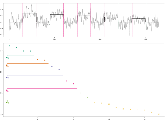
Figure 1: Top: a realisation from (M11) in Appendix D and the piecewise constant mean with $q=10$ change points. Vertical lines denote the change point estimators contained in the candidate model $\widehat{\Theta}_{4}$ which correctly estimates $\Theta$. Bottom: $\mathcal{Y}_{(m)},\,m=1,\ldots,22$ (those associated with $k_{(m)}$ corresponding to the $q$ change points are denoted by circles, the remainder by crosses), along with the sequence of nested models $\widehat{\Theta}_{l},\,l=1,\ldots,5$.

The solution path $\mathcal{P}$ consists of a sequence of candidate change point models $\mathcal{K}_{1}\subset\mathcal{K}_{2}\subset\ldots$ with $\mathcal{K}_{l}:=\{k_{(1)},\ldots,k_{(l)}\}$, which estimate the total number and locations of the mean shifts in $f_{t}$. In this section, we propose a ‘gappy’ candidate model sequence generation step which selects a subset of the above model sequence by discarding candidate models that are not likely to be the final model. More specifically, by the construction of WBS2, which iteratively identifies the local split of the data with the most contrast (max-CUSUM), we expect to observe a large gap between the CUSUM statistics $\mathcal{X}_{(m)}$ computed over those intervals $(s_{(m)},e_{(m)})$ that contain change points well within their interior, and the remaining CUSUMs. Therefore, for the purpose of model selection, we can exploit this large gap in $\mathcal{X}_{(m)},\,1\leq m\leq P$, or equivalently, in $\mathcal{Y}_{(m)}:=\log(\mathcal{X}_{(m)})$; we later show that under some assumptions on the size of changes and the level of noise, the large log-CUSUMs $\mathcal{Y}_{(m)}$ attributed to change points scale as $\log(n)$ while the rest scale as $\log\log(n)$.

For the identification of the large gap in $\mathcal{Y}_{(1)}\geq\ldots\geq\mathcal{Y}_{(P)}$, the simplest approach is to look for the largest difference $\mathcal{Y}_{(m)}-\mathcal{Y}_{(m+1)}$. However, this largest gap may not necessarily correspond to the difference between the max-CUSUMs attributed to mean shifts and spurious ones attributed to fluctuations in the errors, but simply be due to the heterogeneity in the change points (i.e. some changes being more pronounced and therefore easier to detect than others). Figure 1 illustrates this phenomenon where, due to the presence of mean shifts of heterogeneous magnitudes, gaps as large as that between $\mathcal{Y}_{(q)}$ and $\mathcal{Y}_{(q+1)}$ are observed between $\mathcal{Y}_{(m)}$ and $\mathcal{Y}_{(m+1)}$ for $m<q$, although $k_{(m)}$ and $k_{(m+1)}$ for both detect true change points. Therefore, we identify the $M$ largest gaps from $\mathcal{Y}_{(m)}-\mathcal{Y}_{(m+1)},\,1\leq m\leq P-1$, and denote the corresponding indices by $g_{1}<\ldots<g_{M}$ such that

$$\mathcal{Y}_{(g_{l})}-\mathcal{Y}_{(g_{l}+1)}>\mathcal{Y}_{(m)}-\mathcal{Y}_{(m+1)}\quad\text{for all}\quad m\neq g_{l},\,1\leq l\leq M.$$

This returns a sequence of nested models

$$\emptyset=\widehat{\Theta}_{0}\subset\widehat{\Theta}_{1}\subset\ldots\subset\widehat{\Theta}_{M}\subset\{0,\ldots,n-1\}\quad\text{with}\quad\widehat{\Theta}_{l}\setminus\widehat{\Theta}_{l-1}\neq\emptyset\quad\forall\,\,l=1,\ldots,M,$$ (4)

with $\widehat{\Theta}_{l}=\widehat{\Theta}_{l-1}\cup\{k_{(g_{l-1}+1)},\ldots,k_{(g_{l})}\}$. Theorem 2.1 below shows that the model sequence in (4) contains one which consistently detects all $q$ change points with high probability, as is the case in the toy example given in Figure 1. Typically, this gappy model sequence is much sparser than the sequence of all possible models from the solution path and therefore, intuitively, makes our model selection task easier than if we worked with the entire solution path of all nested models. We confirm this point numerically in the simulation studies reported in Appendix D.

2.3 Theoretical properties

In this section, we establish the theoretical properties of the sequence of nested change point models obtained from combining WBS2 with the gappy model sequence generation outlined in Sections 2.1–2.2. The following assumptions are, respectively, on the distribution of $\{Z_{t}\}_{t=1}^{n}$ and the size of changes under $H_{1}:\,q\geq 1$.

Assumption 2.1.

Let $\{Z_{t}\}_{t=1}^{n}$ be a sequence of random variables satisfying $\mathsf{E}(Z_{t})=0$ and $\mathsf{Var}(Z_{t})=\sigma_{Z}^{2}$ with $\sigma_{Z}\in(0,\infty)$. Also, let $\mathsf{P}(\mathcal{Z}_{n})\to 1$ with $\zeta_{n}$ satisfying $\sqrt{\log(n)}=O(\zeta_{n})$ and $\zeta_{n}=O(\log^{\kappa}(n))$ for some $\kappa\in[1/2,\infty)$, where

$\mathcal{Z}_{n}=\left\{\max_{0\leq s<e\leq n}(e-s)^{-1/2}\Big{|}\sum_{t=s+1}^{e}Z_{t}\Big{|}\leq\zeta_{n}\right\}$.

Remark 2.1.

Assumption 2.1 permits $\{Z_{t}\}_{t=1}^{n}$ to have heavier tails than sub-Gaussian such as sub-exponential or sub-Weibull (Vladimirova et al.,, 2020). Appendix G shows that linear time series with short-range dependence and sub-exponential innovations satisfy the assumption, using the Nagaev-type inequality derived in Zhang and Wu, (2017). Similar arguments can be made with the concentration inequalities shown in Doukhan and Neumann, (2007) for weakly dependent time series fulfilling $\mathsf{E}(|Z_{t}|^{k})\leq(k!)^{\nu}C^{k}$ for all $k\geq 1$ and some $\nu\geq 0$ and $C>0$, or in Merlevède et al., (2011) for geometrically strong mixing sequences with sub-exponential tails. Alternatively, under the invariance principle, if there exists (possibly after enlarging the probability space) a standard Wiener process $W(\cdot)$ such that $\sum_{t=1}^{\ell}Z_{t}-W(\ell)=O(\log^{\kappa^{\prime}}(\ell))$ a.s. with $\kappa^{\prime}\geq 1$, then Assumption 2.1 holds with $\zeta_{n}\asymp\log^{\kappa}(n)$ for any $\kappa>\kappa^{\prime}$, where we denote by $a_{n}\asymp b_{n}$ to indicate that $a_{n}=O(b_{n})$ and $b_{n}=O(a_{n})$. Such invariance principles have been derived for dependent data under weak dependence such as mixing (Kuelbs and Philipp,, 1980) and functional dependence measure (Berkes et al.,, 2014) conditions. The increase in $\zeta_{n}$ due to strong serial correlations or heavier tail behaviour, results in a stronger condition on the size of changes for their detection (see Assumptions 2.2 below), as well as possible worsening of the accuracy in change point location estimation (see Theorem 2.1 (i)).

Assumption 2.2.

Let $\delta_{j}=\min(\theta_{j}-\theta_{j-1},\theta_{j+1}-\theta_{j})$ and recall that $f^{\prime}_{j}=f_{\theta_{j}+1}-f_{\theta_{j}}$ for $j=1,\ldots,q$. Then, $\max_{1\leq j\leq q}|f^{\prime}_{j}|=O(1)$. Also, there exists some $c_{1}\in(0,1)$ such that $\min_{1\leq j\leq q}\delta_{j}\geq c_{1}n$, and for some $\varphi>0$, we have $\zeta_{n}^{2}/(\min_{1\leq j\leq q}(f^{\prime}_{j})^{2}\delta_{j})=O(n^{-\varphi})$.

Under Assumption 2.2, we assume that there are finitely many change points with the spacing between the change points increasing linearly in $n$. A similar condition can be found in the literature addressing the problems of change point detection in the presence of serial correlations, see e.g. in Zhao et al., (2022). The upper bound on $|f^{\prime}_{j}|$ is a technical assumption made to distinguish the problem of detecting change points from that of outlier detection, see Cho and Kirch, (2021) for further discussions.

Theorem 2.1.

Let Assumptions 2.1 and 2.2 hold. Suppose that $R_{n}$, the number of intervals at each iteration of WBS2, satisfies

$$R_{n}\geq\frac{9}{8}\left(\frac{n}{\min_{1\leq j\leq q}\delta_{j}}\right)^{2}+1.$$ (5)

Then, on $\mathcal{Z}_{n}$, the following statements hold for $n$ large enough and some $c_{2}\in(0,\infty)$.

1. Let $\widehat{\Theta}[q]=\{\widehat{\theta}_{j},\,1\leq j\leq q:\,\widehat{\theta}_{1}<\ldots<\widehat{\theta}_{q}\}$ denote the set of $q$ change point location estimators corresponding to the $q$ largest max-CUSUMs $\mathcal{X}_{(m)},\,1\leq m\leq q$, obtained as in (3). Then, $\max_{1\leq j\leq q}(f^{\prime}_{j})^{2}|\widehat{\theta}_{j}-\theta_{j}|\leq c_{2}\zeta_{n}^{2}$.

2. The sorted log-CUSUMs $\mathcal{Y}_{(m)}$ satisfy $\mathcal{Y}_{(m)}=\gamma_{m}\log(n)(1+o(1))$ for $m=1,\ldots,q$, while $\mathcal{Y}_{(m)}\leq\kappa_{m}\log\log(n)(1+o(1))$ for $m\geq q+1$, where $\{\gamma_{m}\}_{m=1}^{q}$ and $\{\kappa_{m}\}_{m\geq q+1}$ are non-increasing sequences with $0<\gamma_{m}\leq 1/2$.

Theorem 2.1 (i) establishes that for the solution path $\mathcal{P}$ obtained according to the WCM principle, the entries corresponding to the $q$ largest max-CUSUMs contain the estimators of all $q$ change points $\theta_{j}$ and further, the localisation rate attained by $\widehat{\theta}_{j}$ is minimax optimal up to a logarithmic factor $\zeta_{n}^{2}$ (see e.g. Verzelen et al., (2020)). Statement (ii) shows that the $q$ largest log-CUSUMs are of order $\log(n)$ and are thus distinguished from the rest of the log-CUSUMs bounded as $O(\log\log(n))$. In summary, Theorem 2.1 establishes that the sequence of nested change point models (4) contains the consistent model $\widehat{\Theta}[q]$ as a candidate model provided that $M$ is sufficiently large. We emphasise that Theorem 2.1 is not (yet) a full consistency result for our complete change point estimation procedure – this will be the objective of Section 3. Theorem 2.1 merely indicates that the solution path we obtain contains the correctly estimated model, hence it is in principle possible to extract it with the right model selection tool. Section 3 proposes such a tool.

3 Model selection with gSa

In this section, we discuss how to consistently estimate the number and the locations of change points by choosing an appropriate change point model from the sequence of nested candidate models (4). We propose a new backward elimination-type procedure, referred to as ‘gappy Schwarz algorithm’ (gSa), which makes use of the Schwarz criterion constructed under a parametric assumption imposing an AR structure on $\{Z_{t}\}_{t=1}^{n}$. The novelty of gSa is in the new way in which it applies Schwarz criterion, rather than in the formulation of the information criterion itself. We show the usefulness of gSa when change point model selection is performed simultaneously with the estimation of the serial dependence.

3.1 Schwarz criterion in the presence of autoregressive errors

We assume that $\{Z_{t}\}_{t\in\mathbb{Z}}$ in (1) is a stationary AR process of order $p$, i.e.

$$Z_{t} =\sum_{i=1}^{p}a_{i}Z_{t-i}+\varepsilon_{t}\quad\text{such that}\quad X_{t}=(1-a(B))f_{t}+\sum_{i=1}^{p}a_{i}X_{t-i}+\varepsilon_{t},$$ (6)

where $a(B)=\sum_{i=1}^{p}a_{i}B^{i}$ is defined with the backshift operator $B$. The innovations $\{\varepsilon_{t}\}_{t=1}^{n}$ satisfy $\mathsf{E}(\varepsilon_{t})=0$ and $\mathsf{Var}(\varepsilon_{t})=\sigma_{\varepsilon}^{2}\in(0,\infty)$, and are assumed to have no serial correlations; further assumptions on $\{\varepsilon_{t}\}_{t=1}^{n}$ are made in Assumption 3.1. We denote by $\mu^{\circ}_{j}:=(1-\sum_{i=1}^{p}a_{i})f_{\theta_{j}+1}$ the effective mean level over each interval $\theta_{j}+p+1\leq t\leq\theta_{j+1}$, for $j=0,\ldots,q$, and by $d_{j}=\mu^{\circ}_{j}-\mu^{\circ}_{j-1}$ the effective size of the mean shift correspondingly. Also recall that $\delta_{j}=\min(\theta_{j}-\theta_{j-1},\theta_{j+1}-\theta_{j})$.

In the model selection procedure, we do not assume that the AR order $p$ is known, and its data-driven choice is incorporated into the model selection methodology as described later. For now, suppose that it is set to be some integer $r\geq 0$, and that a change point model is given by a set of candidate change point estimators $\mathcal{A}=\{k_{j},\,1\leq j\leq m:\,k_{1}<\ldots<k_{m}\}\subset\{1,\ldots,n\}$. Then, Schwarz criterion (Schwarz,, 1978) is defined as

$$\text{SC}\left(\{X_{t}\}_{t=1}^{n},\mathcal{A},r\right) =\frac{n}{2}\log\left(\widehat{\sigma}_{n}^{2}\left(\{X_{t}\}_{t=1}^{n},\mathcal{A},r\right)\right)+(|\mathcal{A}|+r)\xi_{n},$$ (7)

where $\widehat{\sigma}_{n}^{2}(\{X_{t}\}_{t=1}^{n},\mathcal{A},r)$ denotes a measure of goodness-of-fit (its precise definition is given below), and a penalty is imposed on the model complexity determined by both the AR order and the number of change points; the requirement on the penalty parameter $\xi_{n}$ in relation to the distribution of $\{\varepsilon_{t}\}_{t\in\mathbb{Z}}$ is discussed in Assumption 3.4 below.

We adopt the residual sum of squares as $\widehat{\sigma}_{n}^{2}(\{X_{t}\}_{t=1}^{n},\mathcal{A},r)$, i.e.

$$\widehat{\sigma}_{n}^{2}(\{X_{t}\}_{t=1}^{n},\mathcal{A},r)=\frac{1}{n}\|\mathbf{Y}-\mathbf{X}\widehat{\bm{\beta}}\|^{2},\quad\text{where}\quad\mathbf{Y}=(X_{1},\ldots,X_{n})^{\top}\quad\text{and}$$

$$\mathbf{X}=\mathbf{X}(\mathcal{A},r)=\begin{bmatrix}\underbrace{\mathbf{L}(r)}_{n\times r}&\underbrace{\mathbf{R}(\mathcal{A})}_{n\times(m+1)}\end{bmatrix}=\left[\begin{array}[]{cccccccc}X_{0}&\cdots&X_{1-r}&1&0&0&\cdots&0\\ \vdots&&&&&&\\ X_{k_{1}-1}&\cdots&X_{k_{1}-r}&1&0&0&\cdots&0\\ X_{k_{1}}&\cdots&X_{k_{1}-r+1}&0&1&0&\cdots&0\\ \vdots&&&\vdots&&&\\ X_{n-1}&\cdots&X_{n-r}&0&0&0&\cdots&1\\ \end{array}\right].$$ (14)

For notational convenience, we assume that $X_{0},\ldots,X_{-r+1}$ are available and their means remain constant such that $\mathsf{E}(X_{t})=\mathsf{E}(X_{1})$ for $t\leq 0$; in practice, we can simply omit the first $p_{\max}$ observations when constructing $\mathbf{Y}$ and $\mathbf{X}$ above, where $p_{\max}$ denotes a pre-specified upper bound on the AR order. The matrix $\mathbf{X}$ is divided into the AR part contained in $\mathbf{L}(r)$ and the deterministic part in $\mathbf{R}(\mathcal{A})$ for modelling mean shifts. We propose to obtain the estimator of regression parameters denoted by $\widehat{\bm{\beta}}=\widehat{\bm{\beta}}(\mathcal{A},r)=(\widehat{\bm{\alpha}}(r)^{\top},\widehat{\bm{\mu}}(\mathcal{A})^{\top})^{\top}$ via least squares estimation, where $\widehat{\bm{\alpha}}(r)\in\mathbb{R}^{r}$ denotes the estimator of the AR parameters and $\widehat{\bm{\mu}}(\mathcal{A})\in\mathbb{R}^{|\mathcal{A}|+1}$ that of the segment-specific levels.

We select the typically unknown AR order $p$ as follows: AR models of varying orders $r\in\{0,\ldots,p_{\max}\}$, are fitted to the data from which we estimate $p$ by

$$\widehat{p}=\widehat{p}(\mathcal{A}) ={\arg\min}_{r\in\{0,\ldots,p_{\max}\}}\,\text{SC}\left(\{X_{t}\}_{t=1}^{n},\mathcal{A},r\right).$$ (15)

In our theoretical analysis, we fully address that the estimator $\widehat{p}(\mathcal{A})$ is used rather than the true AR order $p$.

3.2 gSa: sequential model selection

To demonstrate the main idea, we first address the simpler problem of determining between a given change point model $\mathcal{A}$ and the null model without any change points, and then describe the full procedure for model selection from a sequence of candidate models.

Suppose that the number and locations of mean shifts are consistently estimated by (a subset of) $\mathcal{A}$ in the sense made clear in Assumption 3.2 below, which includes the case of no change point ($q=0$) with the trivial subset $\emptyset\subset\mathcal{A}$. Then, the estimator $\widehat{\bm{\beta}}(\mathcal{A},\widehat{p})=(\widehat{\bm{\alpha}}(\widehat{p})^{\top},\widehat{\bm{\mu}}(\mathcal{A})^{\top})^{\top}$ can be shown to estimate the AR parameters sufficiently well with $\widehat{p}=\widehat{p}(\mathcal{A})$ returned by (15), and the criterion $\text{SC}(\{X_{t}\}_{t=1}^{n},\mathcal{A},\widehat{p})$ gives a suitable indicator of the goodness-of-fit of the change point model $\mathcal{A}$ offset by the increased model complexity. On the other hand, if any change point is ignored in fitting an AR model, the resultant AR parameter estimators over-compensate for the under-specification of mean shifts. In our numerical experiments (reported in Appendix D.3), this often leads to $\text{SC}(\{X_{t}\}_{t=1}^{n},\emptyset,\widehat{p}(\emptyset))$ having a smaller value than $\text{SC}(\{X_{t}\}_{t=1}^{n},\mathcal{A},\widehat{p})$ such that their direct comparison returns the null model even though there are multiple change points present and detected by $\mathcal{A}$.

Instead, we propose to compare $\text{SC}(\{X_{t}\}_{t=1}^{n},\mathcal{A},\widehat{p})$ against

$$\text{SC}_{0}\left(\{X_{t}\}_{t=1}^{n},\widehat{\bm{\alpha}}(\widehat{p})\right):=\frac{n}{2}\log\left(\frac{\left\|(\mathbf{I}-\bm{\Pi}_{\mathbf{1}})\left(\mathbf{Y}-\mathbf{L}(\widehat{p})\widehat{\bm{\alpha}}(\widehat{p})\right)\right\|^{2}}{n}\right)+\widehat{p}\,\xi_{n},$$

where $\mathbf{I}-\bm{\Pi}_{\mathbf{1}}$ denotes the projection matrix removing the sample mean from the right-multiplied vector. By having the plug-in estimator $\widehat{\bm{\alpha}}(\widehat{p})$ from $\widehat{\bm{\beta}}(\mathcal{A},\widehat{p})$ in its definition, $\text{SC}_{0}$ avoids the above-mentioned difficulty arising when evaluating Schwarz criterion at a change point model that under-specifies the number of change points. We conclude that the data is better described by the change point model $\mathcal{A}$ if

$$\text{SC}_{0}\left(\{X_{t}\}_{t=1}^{n},\widehat{\bm{\alpha}}(\widehat{p})\right)>\text{SC}(\{X_{t}\}_{t=1}^{n},\mathcal{A},\widehat{p}),$$ (16)

and if the converse holds, we prefer the null model over the change point model.

This Schwarz criterion-based model selection strategy is extended to be applicable with a sequence of nested change point models $\emptyset=\widehat{\Theta}_{0}\subset\widehat{\Theta}_{1}\subset\ldots\subset\widehat{\Theta}_{M}$ as in (4) even when $M>1$. Referred to as the gappy Schwarz algorithm (gSa) in the remainder of the paper, the proposed methodology performs a backward search along the sequence from the largest model $\widehat{\Theta}_{l}$ with $l=M$, sequentially evaluating whether the reduction in the goodness-of-fit (i.e. increase in the residual sum of squares) by moving from $\widehat{\Theta}_{l}$ to $\widehat{\Theta}_{l-1}$, is sufficiently offset by the decrease in model complexity. More specifically, let $s,e\in\widehat{\Theta}_{l-1}\cup\{0,n\}$ denote two candidates satisfying $\{s+1,\ldots,e-1\}\cap\widehat{\Theta}_{l-1}=\emptyset$, and suppose that $\mathcal{A}=\{s+1,\ldots,e-1\}\cap(\widehat{\Theta}_{l}\setminus\widehat{\Theta}_{l-1})$ is not empty (by definition, $\{s,e\}\subset\widehat{\Theta}_{l}\cup\{0,n\}$). In other words, $\mathcal{A}$ contains candidate estimators detected within the local environment $\{s+1,\ldots,e-1\}$, which appear in $\widehat{\Theta}_{l}$ but do not appear in the smaller models $\widehat{\Theta}_{l^{\prime}},\,l^{\prime}\leq l-1$. Then, we compare $\text{SC}(\{X_{t}\}_{t=s+1}^{e},\mathcal{A},\widehat{p}_{s:e})$ against $\text{SC}_{0}(\{X_{t}\}_{t=s+1}^{e},\widehat{\bm{\alpha}}_{s:e}(\widehat{p}_{s:e}))$ as in (16), with the least squares estimator of the AR parameters $\widehat{\bm{\alpha}}_{s:e}(\widehat{p}_{s:e})$ and its dimension $\widehat{p}_{s:e}$ obtained locally by minimising $\text{SC}(\{X_{t}\}_{t=s+1}^{e},\mathcal{A},r)$ over $r$ (see (15)). If $\text{SC}(\{X_{t}\}_{t=s+1}^{e},\mathcal{A},\widehat{p}_{s:e})<\text{SC}_{0}(\{X_{t}\}_{t=s+1}^{e},\widehat{\bm{\alpha}}_{s:e}(\widehat{p}_{s:e}))$, the change point estimators in $\mathcal{A}$ are deemed as not being spurious; if this is the case for all estimators in $\widehat{\Theta}_{l}\setminus\widehat{\Theta}_{l-1}$, we return $\widehat{\Theta}_{l}$ as the final model.

In our theoretical analysis, when $q\geq 1$, we assume that there exists some $1\leq l^{*}\leq M$ such that $\widehat{\Theta}_{l^{*}}$ correctly detects all change points and nothing else (see Assumption 3.2 below), which is guaranteed by the gappy candidate model sequence generation method described in Section 2. Then with high probability, we have $\text{SC}(\{X_{t}\}_{t=s+1}^{e},\mathcal{A},\widehat{p}_{s:e})<\text{SC}_{0}(\{X_{t}\}_{t=s+1}^{e},\widehat{\bm{\alpha}}_{s:e}(\widehat{p}_{s:e}))$ simultaneously in all local regions $\{s+1,\ldots,e\}$ overlapping with $\widehat{\Theta}_{l^{*}}\setminus\widehat{\Theta}_{l^{*}-1}$. On the other hand, when $l>l^{*}$, we expect to have $\text{SC}(\{X_{t}\}_{t=s+1}^{e},\mathcal{A},\widehat{p}_{s:e})\geq\text{SC}_{0}(\{X_{t}\}_{t=s+1}^{e},\widehat{\bm{\alpha}}_{s:e}(\widehat{p}_{s:e}))$ in all such regions as they contain spurious estimators. Therefore, sequentially examining the nested change point models from the largest model $\widehat{\Theta}_{M}$, gSa returns $\widehat{\Theta}_{l^{*}}$ as the final model with high probability. In its implementation, in the unlikely event of disagreement across the regions containing $\widehat{\Theta}_{l}\setminus\widehat{\Theta}_{l-1}$, we take a conservative approach and conclude that $\widehat{\Theta}_{l}$ contains spurious estimators, and update $l\to l-1$ to repeat the same procedure until some $\widehat{\Theta}_{l},\,l\geq 1$, is selected as the final model, or the null model $\widehat{\Theta}_{0}=\emptyset$ is reached. The full algorithmic description of gSa is provided in Appendix A.2.

In summary, gSa does not directly minimise Schwarz criterion but starting from the largest model, searches for the first largest model $\widehat{\Theta}_{l}$ in which all candidate estimators in $\widehat{\Theta}_{l}\setminus\widehat{\Theta}_{l-1}$ are deemed important as described above. By adopting $\text{SC}_{0}$ for model comparison, it avoids evaluating Schwarz criterion at a candidate model that under-estimates the number of change points (which may lead to loss of power). We show that gSa achieves model selection consistency in the next section.

3.3 Theoretical properties

For the theoretical analysis of gSa, we make a set of assumptions and remark on their relationship to those made in Section 2.3. Assumption 3.1 is imposed on the stochastic part of model (6).

Assumption 3.1.

1. The characteristic polynomial $a(z)=1-\sum_{i=1}^{p}a_{i}z^{i}$ has all of its roots outside the unit circle $|z|=1$.

2. $\{\varepsilon_{t}\}_{t\in\mathbb{Z}}$ is an ergodic and stationary martingale difference sequence with respect to an increasing sequence of $\sigma$-fields $\mathcal{F}_{t}$, such that $\varepsilon_{t}$ and $X_{t}$ are $\mathcal{F}_{t}$-measurable and $\mathsf{E}(\varepsilon_{t}|\mathcal{F}_{t-1})~{}=~{}0$.

3. There exists some $\Delta>0$ such that $\sup_{t}\mathsf{E}(|\varepsilon_{t}|^{2+\Delta}|\mathcal{F}_{t-1})<\infty$ a.s.

4. Let $\mathsf{P}(\mathcal{E}_{n})\to 1$ with $\omega_{n}$ satisfying $\sqrt{\log(n)}=O(\omega_{n})$ and $\omega_{n}^{2}=O(\min_{1\leq j\leq q}\delta_{j})$, where $\delta_{j}=\min(\theta_{j}-\theta_{j-1},\theta_{j+1}-\theta_{j})$ and

   $\mathcal{E}_{n}=\left\{\max_{0\leq s<e\leq n}(e-s)^{-1/2}\Big{|}\sum_{t=s+1}^{e}\varepsilon_{t}\Big{|}\leq\omega_{n}\right\}$.

Assumption 3.1 (i)–(iii) are taken from Lai and Wei, 1982a ; Lai and Wei, 1982b ; Lai and Wei, (1983), where the strong consistency in stochastic regression problems is established. In particular, Condition (i) implies that $\{Z_{t}\}_{t=1}^{n}$ is a short-memory linear process. The term $\omega_{n}$ in Condition (iv) gives a lower bound on the penalty parameter $\xi_{n}$ of Schwarz criterion, see Assumption 3.4. Theorem 1.2A of De la Peña, (1999) derives a Bernstein-type inequality for a martingale difference sequence satisfying $\mathsf{E}(|\varepsilon_{t}|^{k})\leq(k!/2)c_{\varepsilon}^{k}\mathsf{E}(\varepsilon_{t}^{2})$ for all $k\geq 3$ and some $c_{\varepsilon}\in(0,\infty)$, from which we readily obtain $\omega_{n}\asymp\log(n)$. Under a more stringent condition that $\{\varepsilon_{t}\}_{t\in\mathbb{Z}}$ is a sequence of i.i.d. sub-Gaussian random variables, it suffices to set $\omega_{n}\asymp\sqrt{\log(n)}$ (e.g. see Proposition 2.1 (a) of Cho and Kirch, (2022)); Appendix G considers i.i.d. sub-exponential $\{\varepsilon_{t}\}_{t\in\mathbb{Z}}$ for which $\omega_{n}\asymp\log(n)$.

Remark 3.1 (Links between Assumptions 2.1, 2.2 and 3.1).

Assumption 2.1 does not impose any parametric condition on the dependence structure of $\{Z_{t}\}_{t=1}^{n}$. For linear, short memory processes (implied by Assumption 3.1 (i)), Peligrad and Utev, (2006) show that the invariance principle for the linear process is inherited from that of the innovations. Then, as discussed in Remark 2.1, a logarithmic bound $\omega_{n}\asymp\log^{\kappa}(n)$ follows from $\sum_{t=1}^{\ell}\varepsilon_{t}-W(\ell)=O(\log^{\kappa^{\prime}}(n))$ for some $\kappa^{\prime}\in[1,\kappa)$, which in turn leads to $\zeta_{n}\asymp\omega_{n}$. In view of Assumptions 2.1 and 2.2, the condition that $\omega_{n}^{2}=O(\min_{1\leq j\leq q}\delta_{j})$ is a mild one.

We impose the following assumption on the sequence of nested candidate models $\widehat{\Theta}_{0}\subset\ldots\subset\widehat{\Theta}_{M}$, where $\widehat{\Theta}_{l}=\{\widehat{\theta}_{l,j},\,1\leq j\leq\widehat{q}_{l}:\,\widehat{\theta}_{l,1}<\ldots<\widehat{\theta}_{l,\widehat{q}_{l}}\}$ for $l\geq 1$. Recall that $d_{j}$ denotes the effective size of change defined below (6).

Assumption 3.2.

We assume that $\mathsf{P}(\mathcal{M}_{n})\to 1$ where $\mathcal{M}_{n}$ denotes the following event: for a given penalty $\xi_{n}$, we have $\xi_{n}(\min_{0\leq j\leq\widehat{q}_{M}}(\widehat{\theta}_{M,j+1}-\widehat{\theta}_{M,j}))^{-1}=o(1)$ and $\widehat{q}_{M}=|\widehat{\Theta}_{M}|$ is fixed for all $n$. Additionally, there exists some $\rho_{n}\geq 1$ satisfying $(\min_{1\leq j\leq q}d_{j}^{2}\delta_{j})^{-1}\rho_{n}\to 0$, such that under $H_{1}:\,q\geq 1$, there exists $l^{*}\in\{1,\ldots,M\}$ with

$$\widehat{q}_{l^{*}}=q\quad\text{and}\quad\max_{1\leq j\leq q}d_{j}^{2}\left|\widehat{\theta}_{l^{*},j}-\theta_{j}\right|\leq\rho_{n}.$$ (17)

By Theorem 2.1, we have the condition (17) satisfied by the gappy model sequence generated as in (4) with $\rho_{n}\asymp\zeta_{n}^{2}$, where $\zeta_{n}$ is defined in Assumption 2.1. We state this result as an assumption so that if gSa were to be applied with an alternative solution path algorithm other than WBS2, its statistical guarantee is still applicable if the latter satisfied Assumption 3.2. Since the serial dependence structure is learned from the data by fitting an AR model to each segment, the requirement on the minimum spacing of the largest model $\widehat{\Theta}_{M}$ is a natural one and it can be hard-wired into the solution path generation step.

Assumption 3.3 is on the size of changes determined by the effective magnitude of the mean shift $d_{j}$ under (6) and the distance between the change points $\delta_{j}$, and Assumption 3.4 on the choice of the penalty parameter $\xi_{n}$. In particular, the choice of $\xi_{n}$ connects the detectability of change points with the level of noise remaining in the data after accounting for the autoregressive dependence structure.

Assumption 3.3.

$\max_{1\leq j\leq q}|d_{j}|=O(1)$ and $D_{n}:=\min_{1\leq j\leq q}d_{j}^{2}\,\delta_{j}\to\infty$ as $n\to\infty$.

Assumption 3.4.

$\xi_{n}$ satisfies $D_{n}^{-1}\xi_{n}=o(1)$ and $\xi_{n}^{-1}\max(\omega_{n}^{2},\rho_{n})=o(1)$.

By Assumption 3.1 (i), the effective mean shift size $d_{j}$ is of the same order as $f^{\prime}_{j}=f_{\theta_{j}+1}-f_{\theta_{j}}$ since $d_{j}=(1-\sum_{i=1}^{p}a_{i})f^{\prime}_{j}$. Therefore, Assumption 3.3 on the detection lower bound formulated with $d_{j}$, together with Assumption 3.4, is closely related to Assumption 2.2 formulated with $f^{\prime}_{j}$. In fact, we can select $\xi_{n}$ such that Assumption 3.4 follows immediately from Assumption 2.2, recalling that the rate of localisation attained by the latter is $\rho_{n}\asymp\zeta_{n}^{2}$ and $\omega_{n}=O(\zeta_{n})$.

Theorem 3.1.

Let Assumptions 3.1–3.4 hold. Then, on $\mathcal{E}_{n}\cap\mathcal{M}_{n}$, gSa returns $\widehat{\Theta}=\{\widehat{\theta}_{j},\,1\leq j\leq\widehat{q}:\,\widehat{\theta}_{1}<\ldots<\widehat{\theta}_{\widehat{q}}\}$ satisfying

$\widehat{q}=q\quad\text{and}\quad\max_{1\leq j\leq q}d_{j}^{2}\left|\widehat{\theta}_{j}-\theta_{j}\right|\leq\rho_{n}$

for $n$ large enough.

Theorem 3.1 establishes that gSa achieves model selection consistency. Together, Theorems 2.1 and 3.1 lead to the consistency of WCM.gSa, the methodology combining WCM-based gappy model sequence generation and Schwarz criterion-based model selection steps. Once the number of change points and their locations are consistently estimated, we can further improve the location estimators in $\widehat{\Theta}$; Appendix B discusses a simple refinement procedure which achieves the minimax optimal localisation rate.

4 Numerical results

4.1 Simulation results

Appendix C discusses in detail the choice of the tuning parameters for WCM.gSa. We investigate the performance of WCM.gSa on simulated datasets, in comparison with DeCAFS (Romano et al.,, 2022), DepSMUCE (Dette et al.,, 2020) and SNCP (Zhao et al.,, 2022) (the latter two applied with significance level $\alpha=0.05$). Here, we present the results from three representative settings and defer the descriptions of the full simulation results (from thirteen scenarios with varying $n$, change point and serial dependence structures) and the competing methodologies to Appendix D, where we include DepSMUCE and SNCP applied with different choices of $\alpha$ as well as MACE proposed in Wu and Zhou, (2020). There, we also present additional numerical experiments motivating the use of gappy candidate model sequence generation, and investigating the case of very strong autocorrelations.

We generate $1000$ realisations under each setting where $\varepsilon_{t}\sim_{\mbox{\scriptsize{iid}}}\mathcal{N}(0,1)$. In addition to when $f_{t}$ undergoes mean shifts as described below, we also consider the case where $f_{t}$ remains constant to evaluate the size control performance.

1. $f_{t}$ undergoes $q=5$ change points at $(\theta_{1},\theta_{2},\theta_{3},\theta_{4},\theta_{5})=(100,300,500,550,750)$ with $n=1000$ and $(f_{0},f_{1}^{\prime},f_{2}^{\prime},f_{3}^{\prime},f_{4}^{\prime},f_{5}^{\prime})=(0,1,-1,2,-2,-1)$, and $\{Z_{t}\}_{t\in\mathbb{Z}}$ follows an MA($1$) model $Z_{t}=\varepsilon_{t}+b_{1}\varepsilon_{t-1}$ with $b_{1}=-0.9$.

2. $f_{t}$ undergoes $q=5$ change points $\theta_{j}$ as in (M1) with $n=1000$ and $(f_{0},f_{1}^{\prime},f_{2}^{\prime},f_{3}^{\prime},f_{4}^{\prime},f_{5}^{\prime})=(0,5,-3,6,-7,-3)$, and $\{Z_{t}\}_{t\in\mathbb{Z}}$ follows an ARMA($2$, $6$) model: $Z_{t}=0.75Z_{t-1}-0.5Z_{t-2}+\varepsilon_{t}+0.8\varepsilon_{t-1}+0.7\varepsilon_{t-2}+0.6\varepsilon_{t-3}+0.5\varepsilon_{t-4}+0.4\varepsilon_{t-5}+0.3\varepsilon_{t-6}$.

3. $f_{t}$ undergoes $q=15$ change points at $\theta_{j}=\lceil nj/16\rceil$ with $n=2000$, where the level parameters $f_{\theta_{j}+1}$ are generated uniformly as $(-1)^{j}\cdot f_{\theta_{j}+1}\sim_{\mbox{\scriptsize{iid}}}\mathcal{U}(1,2)$ for each realisation. $\{Z_{t}\}_{t\in\mathbb{Z}}$ follows an AR($1$) model: $Z_{t}=a_{1}Z_{t-1}+\sqrt{1-a_{1}^{2}}\varepsilon_{t}$ with $a_{1}=0.9$.

Table 1 summarises the simulation results; see Table LABEL:table:sim:h1 in Appendix for the full results where the exact definitions of RMSE and $d_{H}$ can be found. Overall, across the various scenarios, WCM.gSa performs well both when $q=0$ and $q\geq 1$. In particular, the proportion of the realisations where WCM.gSa detects spurious estimators in the absence of any mean shift is close to $0$. Controlling for the size, especially in the presence of serial correlations, is a difficult task and as shown below, competing methods fail to do so by a large margin in some scenarios. When $q\geq 1$, WCM.gSa performs well in most scenarios according to a variety of criteria, such as model selection accuracy measured by $|\widehat{q}-q|$ or the localisation accuracy measured by $d_{H}$. We highlight the importance of the gappy model sequence generation step of Section 2.2: see the results reported under ‘no gap’ which refers to a procedure that omits this step from WCM.gSa and applies the Schwarz criterion-based model selection procedure directly to the model sequence consisting of consecutive entries from the WBS2-generated solution path. It suffers from having to perform a large number of model comparison steps and tends to over-estimate the number of change points in some scenarios.

DepSMUCE occasionally suffers from a calibration issue; in order not to detect spurious change points, it requires $\alpha$ to be set conservatively but for improved detection power, a larger $\alpha$ is better. In addition, the estimator of the LRV proposed therein tends to under-estimate the LRV when it is close to zero as in (M1), or when there are strong autocorrelations as in (M3), thus incurring a large number of falsely detected change points. Similar sensitivity to the choice of $\alpha$ is observable from SNCP. In addition, it tends to return spurious change point estimators when $q=0$ in the presence of strong autocorrelations as in (M3), while under-detecting change points when $q\geq 1$ in some scenarios.

DeCAFS operates under the assumption that $\{Z_{t}\}_{t=1}^{n}$ is an AR($1$) process. Therefore, it is applied under model mis-specification in some scenarios, but still performs reasonably well in not returning false positives. The exception is (M3) where, in the presence of strong autocorrelations, it returns spurious estimators over $50\%$ of realisations even though the model is correctly specified in this scenario. Its detection accuracy suffers under model mis-specification in some scenarios such as (M1) and (M2) when compared to WCM.gSa, but DeCAFS tends to attain good MSE.

Table 1: We report the proportion of returning $\widehat{q}\geq 1$ when $q=0$ (size) and the summary of estimated change points when $q>1$ according to the distribution of $\widehat{q}-q$, relative MSE (RMSE) and the Hausdorff distance ($d_{H}$) over $1000$ realisations. Methods that control the size at $0.05$, and that achieve the best performance when $q>1$ according to different criteria, are highlighted in bold for each scenario.

			$\widehat{q}-q$
Model	Method	Size	$\geq-3$	$-2$	$-1$	$0$	$1$	$2$	$3\leq$	RMSE	$d_{H}$
(M1)	WCM.gSa	0.000	0.000	0.000	0.000	1.000	0.000	0.000	0.000	68.720	1.988
	no gap	0.000	0.000	0.000	0.000	1.000	0.000	0.000	0.000	68.720	1.988
	DepSMUCE	1.000	0.000	0.000	0.000	0.485	0.167	0.163	0.185	219.196	48.359
	DeCAFS	0.064	0.000	0.006	0.029	0.742	0.148	0.053	0.022	304.694	26.274
	SNCP	0.000	0.000	0.000	0.000	1.000	0.000	0.000	0.000	35.512	1.06
(M2)	WCM.gSa	0.001	0.000	0.000	0.019	0.873	0.092	0.014	0.002	4.907	34.627
	no gap	0.020	0.002	0.002	0.012	0.178	0.024	0.037	0.745	11.030	148.765
	DepSMUCE	0.031	0.052	0.385	0.429	0.134	0.000	0.000	0.000	18.567	145.406
	DeCAFS	0.099	0.006	0.035	0.137	0.773	0.049	0.000	0.000	3.891	61.517
	SNCP	0.084	0.117	0.293	0.372	0.215	0.002	0.001	0.000	15.428	166.724
(M3)	WCM.gSa	0.000	0.087	0.177	0.233	0.319	0.076	0.041	0.067	3.184	86.139
	no gap	0.058	0.000	0.000	0.000	0.000	0.000	0.000	1.000	4.498	92.759
	DepSMUCE	0.936	0.767	0.153	0.070	0.010	0.000	0.000	0.000	8.655	139.298
	DeCAFS	0.565	0.000	0.004	0.019	0.755	0.203	0.017	0.002	1.065	19.751
	SNCP	0.258	0.956	0.034	0.007	0.003	0.000	0.000	0.000	11.698	290.266

4.2 Nitrogen oxides concentrations in London

NO_x is a generic term for the nitrogen oxides that are the most relevant for air pollution, namely nitric oxide (NO) and nitrogen dioxide (NO₂). The main anthropogenic sources of NO_x are mobile and stationary combustion sources, and its acute and chronic health effects have been well-documented (Kampa and Castanas,, 2008). We analyse the daily average concentrations of NO₂ and NO_x measured (in $\mu$g$/$m³) at Marylebone Road in London, U.K., from September 1, 2000 to September 30, 2020; the datasets were retrieved from Defra (https://uk-air.defra.gov.uk/). The concentration measurements are positive integers and exhibit seasonality and weekly patterns as well as distinguished behaviour on bank holidays, since road traffic is the principal outdoor source of NO_x in a busy London road. To correct for possible heavy-tailedness of the raw measurements, we take the square root transform and further remove seasonal and weekly trends and bank holiday effects from the transformed data using a model trained on the observations from January 2004 to December 2010; for details of the pre-processing steps, see Appendix E.1. The resulting time series are plotted in Figure 2, where it is also seen that the thus-transformed data exhibit persistent autocorrelations.

We analyse the transformed time series from NO₂ and NO_x concentrations for change points in the level, with the tuning parameters for WCM.gSa chosen as recommended in Appendix C apart from $M$, the number of candidate models considered; given the large number of observations ($n=7139$), we allow for $M=10$ instead of the default choice $M=5$. The change points detected by WCM.gSa are plotted in Figure 2. For comparison, we also report the change points estimated by DepSMUCE and DeCAFS, see Table 2.

Figure 2 shows that a good deal of autocorrelations remain in the data after removing the estimated mean shifts, but the persistent autocorrelations are no longer observed. This supports the hypothesis that the (de-trended and transformed) NO₂ and NO_x concentrations over the period in consideration, can plausibly be accounted for by a model with short-range dependence and multiple mean shifts; we refer to Mikosch and Stărică, (2004), Berkes et al., (2006) Yau and Davis, (2012) and Norwood and Killick, (2018) for discussions on how weakly dependent time series with mean shifts may appear as a long-range dependent time series. In Appendix E.2, we further validate the set of change point estimators detected by WCM.gSa from the NO₂ time series, by attempting to remove the bulk of serial dependence from the data and then applying an existing procedure for change point detection for uncorrelated data.

Figure 2: First (third) panel: daily average concentrations of NO₂ (NO_x) after transformation and de-trending, plotted together with the change points detected by WCM.gSa (vertical lines) and estimated piecewise constant mean (bold lines). Second (fourth) panel: autocorrelation function of transformed and de-trended NO₂ (NO_x) without (left) and with (right) the time-varying mean adjusted.

Table 2: Change points detected from the daily average concentrations of NO₂ and NO_x measured at Marylebone Road in London from September 1, 2000 to September 30, 2020. Any location estimators commonly detected from both NO₂ and NO_x concentrations (within $10$ days from one another) by each method are highlighted in bold. For DepSMUCE, parameterised by the significance level $\alpha$, identical estimators are returned with either of $\alpha\in\{0.05,0.2\}$.

Method	NO2	NOx
WCM.gSa	2003-01-31, 2007-03-17, 2007-11-15,	2001-03-15, 2018-05-13,
	2008-10-26, 2010-07-25, 2018-10-13,	2019-03-22, 2020-03-18
	2019-03-30, 2020-03-18
DepSMUCE	2003-01-31, 2010-07-25,	2001-03-15, 2018-05-13,
	2018-10-14, 2020-03-18	2020-03-18
DeCAFS	2003-02-05, 2005-12-11, 2005-12-17	2001-11-07, 2001-11-09, 2005-12-08
	2007-04-25, 2007-05-05, 2007-12-10	2005-12-11, 2005-12-17, 2008-12-06
	2008-03-03, 2008-03-04, 2009-09-08	2008-12-08, 2018-05-13, 2020-03-18
	2009-09-20, 2012-10-20, 2012-10-27
	2018-10-14, 2020-03-18

In February 2003, a programme of traffic management measures was introduced in central London including the installation of particulate traps on most London buses and other heavy duty diesel vehicles, which convert NO in the exhaust stream to NO₂ and thus bring in the increase of primary NO₂ emissions from such vehicles (Air Quality Expert Group,, 2004). This accounts for the prominent increase in the concentration of NO₂ detected around January 2003 by WCM.gSa (also by DepSMUCE and DeCAFS) which, however, is not observed from NO_x, since the latter contains the combined concentrations of NO and NO₂. The two series share the common change point detected at the end of March 2019 (not detected by DepSMUCE or DeCAFS). The Ultra Low Emission Zone in central London was launched on 8 April 2019, which includes Marylebone Road where the measurements were taken, and its introduction coincides with the decline in the concentrations of both NO₂ and NO_x. Another common change point is detected on March 18, 2020 (also detected by DepSMUCE and DeCAFS) which confirms that the nation-wide COVID-19 lockdown on March 23, 2020 led to the substantial reduction of NO_x levels across the country (Higham et al.,, 2020).

Appendix A Algorithms

A.1 Wild Binary Segmentation 2 algorithm

Algorithm 1 provides a pseudo code for the Wild Binary Segmentation 2 (WBS2) algorithm proposed in Fryzlewicz, 2020a .

We remark that WBS2 as defined in Fryzlewicz, 2020a uses random sampling in line 7 of Algorithm 1, but our preference is for deterministic sampling as it generates reproducible results without having to fix a random seed. To obtain at least $\widetilde{R}$ intervals over an equispaced (or almost equispaced, if exactly equal spacing is not possible) grid on a generic interval $[s,e]$, we firstly select the smallest integer $\widetilde{K}$ for which the number of all intervals with start- and end-points in the set $\{1,\ldots,\widetilde{K}\}$ equals or exceeds $\widetilde{R}$. Next, we map (linearly with rounding) the integer grid $[1,\widetilde{K}]$ onto an integer grid within $[s,e]$, as $j\to[\frac{e-s}{\widetilde{K}-1}j+s-\frac{e-s}{\widetilde{K}-1}]$ for each $j\in\{1,\ldots,\widetilde{K}\}$, where $[\cdot]$ represents rounding to the nearest integer. We then use all start- and end-points on the resulting grid to obtain the required collection $(s_{m},e_{m})$ in line 7 of Algorithm 1.

Input: Data $\{X_{t}\}_{t=1}^{n}$, the number of intervals $R_{n}$

Function $\textnormal{{wbs2}}(\{X_{t}\}_{t=1}^{n},R_{n},s,e)$:

       if $e-s\leq 1$ then $\textnormal{{return}}\,\emptyset$

      

      Let $\mathcal{A}_{s,e}\leftarrow\{(\ell,r)\in\mathbb{Z}^{2}:\,s\leq\ell<r\leq e\text{ and }r-\ell>1\}$

      if $|\mathcal{A}_{s,e}|\leq R_{n}$ then

             $\widetilde{R}\leftarrow|\mathcal{A}_{s,e}|$ and set $\mathcal{R}_{s,e}\leftarrow\mathcal{A}_{s,e}$

       else

            $\widetilde{R}\leftarrow R_{n}$ and draw $\widetilde{R}$ elements from $\mathcal{A}_{s,e}$ deterministically over an equispaced grid, to form $\mathcal{R}_{s,e}=\{1\leq m\leq\widetilde{R}:\,(s_{m},e_{m})\}$

       end if

      

      Identify $(s_{\circ},k_{\circ},e_{\circ})=\arg\max_{(s_{m},k,e_{m}):\,1\leq m\leq\widetilde{R},\,s_{m}<k<e_{m}}|\mathcal{X}_{s_{m},k,e_{m}}|$

      return   $(s_{\circ},k_{\circ},e_{\circ},|\mathcal{X}_{s_{\circ},k_{\circ},e_{\circ}}|)\cup\textnormal{{wbs2}}(\{X_{t}\}_{t=1}^{n},R_{n},s,k_{\circ})\cup\textnormal{{wbs2}}(\{X_{t}\}_{t=1}^{n},R_{n},k_{\circ},e)$

$\mathcal{P}_{0}\leftarrow\textnormal{{wbs2}}(\{X_{t}\}_{t=1}^{n},R_{n},0,n)$

Output: $\mathcal{P}_{0}$

Algorithm 1 Wild Binary Segmentation 2

A.2 Gappy Schwarz algorithm

For each $l\geq 1$, we denote $\widehat{\Theta}_{l}=\{\widehat{\theta}_{l,j},\,1\leq j\leq\widehat{q}_{l}:\,\widehat{\theta}_{l,1}<\ldots<\widehat{\theta}_{l,\widehat{q}_{l}}\}$, and adopt the notational convention that $\widehat{\theta}_{l,0}=0$ and $\widehat{\theta}_{l,\widehat{q}_{l}+1}=n$. Initialised with $l=M$, gSa performs the following steps.

1. We identify $u\in\{0,\ldots,\widehat{q}_{l-1}\}$ with $\{\widehat{\theta}_{l-1,u}+1,\ldots,\widehat{\theta}_{l-1,u+1}-1\}\cap\widehat{\Theta}_{l}\neq\emptyset$; that is, the segment $\{\widehat{\theta}_{l-1,u}+1,\ldots,\widehat{\theta}_{l-1,u+1}-1\}$ defined by the consecutive elements of $\widehat{\Theta}_{l-1}$, has additional change points detected in $\widehat{\Theta}_{l}$ such that $\{\widehat{\theta}_{l-1,u}+1,\ldots,\widehat{\theta}_{l-1,u+1}-1\}\cap(\widehat{\Theta}_{l}\setminus\widehat{\Theta}_{l-1})\neq\emptyset$. By construction, the set of such indices, $\mathcal{I}_{l}:=\{u_{1},\ldots,u_{q^{\prime}_{l}}\}$, satisfies $|\mathcal{I}_{l}|\geq 1$. For each $u_{v},\,v=1,\ldots,q^{\prime}_{l}$, we repeat the following steps with a logical vector of length $q^{\prime}_{l}$, $\mathbf{F}\in\{\text{\tt TRUE},\text{\tt FALSE}\}^{q^{\prime}_{l}}$, initialised as $\mathbf{F}=(\text{\tt TRUE}.\ldots,\text{\tt TRUE})$.

   1. Setting $\mathcal{A}=\{\widehat{\theta}_{l-1,u_{v}}+1,\ldots,\widehat{\theta}_{l-1,u_{v}+1}-1\}\cap\widehat{\Theta}_{l}$, obtain $\widehat{p}$ that returns the smallest $\text{SC}(\{X_{t}\}_{t=\widehat{\theta}_{l-1,u_{v}}+1}^{\widehat{\theta}_{l-1,u_{v}+1}},\mathcal{A},r)$ over $r\in\{0,\ldots,p_{\max}\}$ as outlined in (15), and the corresponding AR parameter estimator $\widehat{\bm{\alpha}}(\widehat{p})$ via least squares estimation.

   2. If $\text{SC}(\{X_{t}\}_{t=\widehat{\theta}_{l-1,u_{v}}+1}^{\widehat{\theta}_{l-1,u_{v}+1}},\mathcal{A},\widehat{p})<\text{SC}_{0}(\{X_{t}\}_{t=\widehat{\theta}_{l-1,u_{v}}+1}^{\widehat{\theta}_{l-1,u_{v}+1}},\widehat{\bm{\alpha}}(\widehat{p}))$, update $F_{v}\leftarrow{\tt FALSE}$.

2. If some elements of $\mathbf{F}$ satisfy $F_{v}=\text{\tt TRUE}$ and $l>1$, update $l\leftarrow l-1$ and go to Step 1. If $F_{v}=\text{\tt FALSE}$ for all $v=1,\ldots,q^{\prime}_{l}$, return $\widehat{\Theta}_{l}$ as the set of change point estimators. Otherwise, return $\widehat{\Theta}_{0}=\emptyset$.

Theorem 3.1 shows that we have either $F_{v}=\text{\tt FALSE}$ for all $v=1,\ldots,q^{\prime}_{l}$ when the corresponding $\widehat{\Theta}_{l}=\widehat{\Theta}_{l^{*}}$ (see Assumption 3.2 for the definition of $\widehat{\Theta}_{l^{*}}$), or $F_{v}=\text{\tt TRUE}$ for all $v$ when $l>l^{*}$ and thus all $\widehat{\Theta}_{l}\setminus\widehat{\Theta}_{l-1}$ are spurious estimators. In implementing the methodology, we take a conservative approach in the above Step 2, to guard against the unlikely event where the output $\mathbf{F}$ contains mixed results.

Appendix B Refinement of change point estimators

Throughout this section, we condition on the event that $\widehat{\Theta}[q]$ is chosen at the model selection step, and discuss how the location estimators can further be refined; consistent model selection based on the estimators of change point locations returned directly by WBS2 (without any additional refinement), is discussed in Section 3.

By Theorem 2.1 and Assumption 2.2, each $\widehat{\theta}_{j},\,1\leq j\leq q$, is sufficiently close to the corresponding change point $\theta_{j}$ in the sense that $|\widehat{\theta}_{j}-\theta_{j}|\leq(f_{j}^{\prime})^{-2}\rho_{n}\leq c\delta_{j}$ for some $c\in(0,1/6)$ with probability tending to one, for $n$ large enough. Defining $\ell_{1}=0$, $r_{q}=n$,

$$\ell_{j}=\left\lfloor\frac{2}{3}\widehat{\theta}_{j-1}+\frac{1}{3}\widehat{\theta}_{j}\right\rfloor,\quad j=2,\ldots,q,\quad\text{and}\quad r_{j}=\left\lfloor\frac{1}{3}\widehat{\theta}_{j}+\frac{2}{3}\widehat{\theta}_{j+1}\right\rfloor,\quad j=1,\ldots,q-1,$$

we have each interval $(\ell_{j},r_{j})$ sufficiently large and contain a single change point $\theta_{j}$ well within its interior, i.e.

$$\min(\theta_{j}-\ell_{j},r_{j}-\theta_{j}) \geq(2/3-c)\delta_{j}>\delta_{j}/2,\quad\text{and}$$ (B.1)

$$\min(\ell_{j}-\theta_{j-1},\theta_{j+1}-r_{j}) \geq(1/3-c)\delta_{j}>0.$$ (B.2)

Then, we propose to further refine the location estimator $\widehat{\theta}_{j}$ by $\check{\theta}_{j}={\arg\max}_{\ell_{j}<k<r_{j}}\left|\mathcal{X}_{\ell_{j},k,r_{j}}\right|$, which generally improves the localisation rate. To see this, we impose the following assumption on the error distribution which, by its formulation, trivially holds under Assumption 2.1 with $\widetilde{\zeta}_{n}=\zeta_{n}$. However, we often have the assumption met with a much tighter bound as discussed in Remark B.1, which leads to the improvement in the localisation rate of the refined estimators $\check{\theta}_{j}$ as shown in Proposition B.1.

Assumption B.1.

For any sequence $1\leq a_{n}\leq\min_{1\leq j\leq q}(f_{j}^{\prime})^{2}\delta_{j}$ and some $\widetilde{\zeta}_{n}$ satisfying $\widetilde{\zeta}_{n}=O(\zeta_{n})$ (with $\zeta_{n}$ as in Assumption 2.1), let $\mathsf{P}(\widetilde{\mathcal{Z}}_{n})\to 1$ where

$$\widetilde{\mathcal{Z}}_{n} =\left\{\max_{1\leq j\leq q}\;\max_{(f_{j}^{\prime})^{-2}a_{n}\leq\ell\leq\theta_{j}-\theta_{j-1}}\frac{\sqrt{(f_{j}^{\prime})^{-2}a_{n}}}{\ell}\left|\sum_{t=\theta_{j}-\ell+1}^{\theta_{j}}Z_{t}\right|\leq\widetilde{\zeta}_{n}\right\}$$

$$\qquad\bigcap\left\{\max_{1\leq j\leq q}\;\max_{(f_{j}^{\prime})^{-2}a_{n}\leq\ell\leq\theta_{j+1}-\theta_{j}}\frac{\sqrt{(f_{j}^{\prime})^{-2}a_{n}}}{\ell}\left|\sum_{t=\theta_{j}+1}^{\theta_{j}+\ell}Z_{t}\right|\leq\widetilde{\zeta}_{n}\right\}.$$

Proposition B.1.

Let the assumptions of Theorem 2.1 and Assumption B.1 hold. Then, there exists $c_{3}\in(0,\infty)$ such that

$$\mathsf{P}\left(\max_{1\leq j\leq q}(f_{j}^{\prime})^{2}|\check{\theta}_{j}-\theta_{j}|\leq c_{3}(\widetilde{\zeta}_{n})^{2}\right)\geq\mathsf{P}\left(\mathcal{Z}_{n}\cap\widetilde{\mathcal{Z}}_{n}\right)\to 1.$$

Remark B.1.

When the number of change points $q$ is bounded, Assumption B.1 holds with $\widetilde{\zeta}_{n}$ diverging at an arbitrarily slow rate, provided that

$$\mathsf{E}\left|\sum_{t=l+1}^{r}Z_{t}\right|^{\nu}\leq C(r-l)^{\nu/2}\quad\text{for any}\quad-\infty<l<r<\infty$$ (B.3)

for some constant $C>0$ and $\nu>2$, see Proposition 2.1 (c.ii) of Cho and Kirch, (2022). The condition (B.3) is satisfied by many time series models, see Appendix B.2 in Kirch, (2006) and the references therein. On the other hand, Theorem 1 of Shao and Zhang, (2010) indicates that the lower bound $\sqrt{\log(n)}=O(\zeta_{n})$ cannot be improved. Therefore, Proposition B.1 shows that the extra step indeed improves upon the localisation rate attained by the WBS2 reported in Theorem 2.1 (i). In fact, for time series models satisfying (B.3), the refinement leads to $(f_{j}^{\prime})^{2}|\check{\theta}_{j}-\theta_{j}|=O_{p}(1)$, thus matching the minimax optimal rate of multiple change point localisation (see Proposition 6 of Verzelen et al., (2020)).

Appendix C Implementation and the choice of tuning parameters

In line with the condition (5) and Assumption 3.2, we set $Q_{n}=\lfloor\log^{1.9}(n)\rfloor$, which imposes an upper bound on the number of change points. In simulation studies where test signals with $n\geq 2000$ are considered, we select $M=5$, i.e. we generate a sequence of $M=5$ nested change point models (in addition to the null model) to be considered by the model selection methodology. In real data analysis in Section 4.2 with $n\approx 7000$, we select $M=10$. Generally, with greater $M$, there is more chance for the second stage gSa to ‘make a mistake’, since there are more candidate models in consideration. On the other hand, if $M$ is chosen too small, we may not have a candidate model that fulfils Assumption 3.2 as discussed in Section 2.2 when motivating the gappy model sequence generation. In view of this, we recommend to select $M$ based on the length of the data. By default, the number of intervals drawn by the deterministic sampling in Algorithm 1 is set at $R_{n}=100$, and the maximum AR order is set at $p_{\max}=10$ unless stated otherwise when input time series is short. To ensure that there are enough observations over each interval defined by two adjacent candidate change point estimators for numerical stability, we set the minimum spacing to be $\max(20,p_{\max}+\lceil\log(n)\rceil)$ and feed this into Algorithm 1 in the solution path generation. Finally, the penalty of SC is given by $\xi_{n}=\log^{1.01}(n)$ which is in accordance with Assumption 3.4 when the innovations $\{\varepsilon_{t}\}$ are distributed as (sub-)Gaussian random variables such that $\omega_{n}\asymp\sqrt{\log(n)}$ fulfils Assumption 3.1 (iv).

Appendix D Complete simulation studies

In this section, we present the complete simulation results summarised in Section 4.1 of the main text.

D.1 Set-up

We consider a variety of data generating processes for $\{X_{t}\}$; in the following, we assume $\varepsilon_{t}\sim_{\mbox{\scriptsize{iid}}}\mathcal{N}(0,\sigma_{\varepsilon}^{2})$ with $\sigma_{\varepsilon}=1$ unless stated otherwise. In addition to (M1)–(M3), we simulate datasets under the following scenarios. We also consider the case where $f_{t}=0$ in each setting, to evaluate the size control performance of the methods considered in the comparative simulation study (their descriptions are given below the list of data generating processes).

1. $f_{t}$ undergoes $q=5$ change points at $(\theta_{1},\theta_{2},\theta_{3},\theta_{4},\theta_{5})=(100,300,500,550,750)$ with $n=1000$ and $(f_{0},f_{1}^{\prime},f_{2}^{\prime},f_{3}^{\prime},f_{4}^{\prime},f_{5}^{\prime})=(0,1,-1,2,-2,-1)$, and $Z_{t}=\varepsilon_{t}$.

2. $f_{t}$ undergoes $q=2$ change points at $(\theta_{1},\theta_{2})=(75,125)$ with $n=200$ and $(f_{0},f_{1}^{\prime},f_{2}^{\prime})=(0,2.5,-2.5)$, and $\{Z_{t}\}_{t\in\mathbb{Z}}$ follows an ARMA($1,1$) model: $Z_{t}=a_{1}Z_{t-1}+\varepsilon_{t}+b_{1}\varepsilon_{t}$ with $a_{1}=0.5$, $b_{1}=0.3$ and $\sigma_{\varepsilon}=1/2.14285$.

3. $f_{t}$ undergoes $q=2$ change points at $(\theta_{1},\theta_{2})=(50,100)$ with $n=150$ and $(f_{0},f_{1}^{\prime},f_{2}^{\prime})=(0,2.5,-2.5)$, and $\{Z_{t}\}_{t\in\mathbb{Z}}$ follows an AR($1$) model: $Z_{t}=a_{1}Z_{t-1}+\varepsilon_{t}$ with $a_{1}=0.5$ and $\sigma_{\varepsilon}=\sqrt{1-a_{1}^{2}}$.

4. $f_{t}$ undergoes $q=2$ change points at $(\theta_{1},\theta_{2})=(100,200)$ with $n=300$ and $(f_{0},f_{1}^{\prime},f_{2}^{\prime})=(0,1,-1)$, and $\{Z_{t}\}_{t\in\mathbb{Z}}$ follows an ARMA($1$, $1$) model: $Z_{t}=a_{1}Z_{t-1}+\varepsilon_{t}+b_{1}\varepsilon_{t-1}$ with the ARMA parameters are generated as $a_{1},b_{1}\sim_{\mbox{\scriptsize{iid}}}\mathcal{U}(-0.9,0.9)$ for each realisation, and $\sigma_{\varepsilon}=\sqrt{(1-a_{1}^{2})/(1+a_{1}b_{1}+b_{1}^{2})}$.

5. $f_{t}$ undergoes $q=5$ change points at $(\theta_{1},\theta_{2},\theta_{3},\theta_{4},\theta_{5})=(100,300,500,550,750)$ with $n=1000$ and $(f_{0},f_{1}^{\prime},f_{2}^{\prime},f_{3}^{\prime},f_{4}^{\prime},f_{5}^{\prime})=(0,1,-1,2,-2,-1)$, and $\{Z_{t}\}_{t\in\mathbb{Z}}$ follows an MA($1$) model $Z_{t}=\varepsilon_{t}+b_{1}\varepsilon_{t-1}$ with $b_{1}=0.3$.

6. $f_{t}$ undergoes $q=5$ change points as in (M4) with $n=1000$ and $(f_{0},f_{1}^{\prime},f_{2}^{\prime},f_{3}^{\prime},f_{4}^{\prime},f_{5}^{\prime})=(0,3,-3,4,-4,-3)$, and $\{Z_{t}\}_{t\in\mathbb{Z}}$ follows an MA($4$) model: $Z_{t}=\varepsilon_{t}+0.9\varepsilon_{t-1}+0.8\varepsilon_{t-2}+0.7\varepsilon_{t-3}+0.6\varepsilon_{t-4}$.

7. $f_{t}$ undergoes $q=15$ change points at $\theta_{j}=\lceil nj/16\rceil$, $j=1,\ldots,15$ with $n=2000$, where the level parameters $f_{\theta_{j}+1}$ are generated uniformly as $(-1)^{j}\cdot f_{\theta_{j}+1}\sim_{\mbox{\scriptsize{iid}}}\mathcal{U}(1,2),\,j=0,\ldots,15$, for each realisation. $\{Z_{t}\}_{t\in\mathbb{Z}}$ follows an AR($1$) model as in (M6) with $a_{1}=0.5$.

8. $f_{t}$ undergoes $q=10$ change points at $\theta_{j}=150j$, $j=1,\ldots,10$ with $n=1650$ and $(f_{0},f^{\prime}_{1},f^{\prime}_{2},f^{\prime}_{3},f^{\prime}_{4},f^{\prime}_{5},f^{\prime}_{6},f^{\prime}_{7},f^{\prime}_{8},f^{\prime}_{9},f^{\prime}_{10})=(0,7,-7,6,-6,5,-5,4,-4,3,-3)$, and $\{Z_{t}\}_{t\in\mathbb{Z}}$ follows an ARMA($2$, $6$) model as in (M2).

9. $f_{t}$ is as in (M4) and $\{Z_{t}\}_{t\in\mathbb{Z}}$ follows a time-varying AR($1$) model: $Z_{t}=a_{1}(t)Z_{t-1}+\sigma(t)\varepsilon_{t}$ with $a_{1}(t)=0.5-0.2\cos(2\pi t/n)$ and $\sigma(t)=\sqrt{1-a_{1}(t)^{2}}$.

10. $f_{t}$ is as in (M4) and $\{Z_{t}\}_{t\in\mathbb{Z}}$ follows a time-varying AR($1$) model: $Z_{t}=a_{1}(t)Z_{t-1}+\sigma(t)\varepsilon_{t}$ where $a_{1}(t)$ is piecewise constant with change points at $\theta_{j},\,j=1,\ldots,q$ such that $a_{1}(t)=0.3\mathbb{I}_{t\leq\theta_{1}}+0.4\mathbb{I}_{\theta_{1}<t\leq\theta_{2}}+0.6\mathbb{I}_{\theta_{2}<t\leq\theta_{3}}+0.7\mathbb{I}_{\theta_{3}<t\leq\theta_{4}}+0.5\mathbb{I}_{\theta_{4}<t\leq\theta_{5}}+0.3\mathbb{I}_{t>\theta_{5}}$ and $\sigma(t)=\sqrt{1-a_{1}(t)^{2}}$.

Apart from Model (M4), all others model have serial correlations in $\{Z_{t}\}_{t=1}^{n}$. Models (M5) (motivated by an example in Wu and Zhou, (2020)), (M6) and (M7) consider relatively short time series with $n\in[150,300]$. Models (M2), (M8) and (M9) are taken from Dette et al., (2020). In (M1), the LRV is close to zero and thus its accurate estimation is difficult. Models (M3) and (M10) have a teeth-like signal containing frequent change points and the underlying $\{Z_{t}\}_{t\in\mathbb{Z}}$ has strong autocorrelations in (M3), and (M11) considers frequent, heterogeneous changes in the mean. In Models (M12) and (M13), the noise $\{Z_{t}\}_{t=1}^{n}$ has time-varying serial dependence structure.

We generate $1000$ realisations under each model. For each scenario, we additionally consider the case in which $f_{t}\equiv 0$ (thus $q=0$) in order to evaluate the proposed methodology on its size control. On each realisation, we apply the proposed WCM.gSa with the tuning parameters are selected as described in Section C. For comparison, we consider a procedure that omits the gappy model sequence generation step from WCM.gSa: referred to as ‘no gap’, it applies the SC-based model selection procedure directly to the model sequence consisting of consecutive entries from the WBS2-generated solution path.

We include DepSMUCE (Dette et al.,, 2020), DeCAFS (Romano et al.,, 2022), MACE (Wu and Zhou,, 2020) and SNCP (Zhao et al.,, 2022) in the simulation studies. DepSMUCE extends the SMUCE procedure (Frick et al.,, 2014) proposed for independent data, by estimating the LRV using a difference-type estimator. MACE is a multiscale moving sum-based procedure with self-normalisation-based scaling that accounts for serial correlations. SNCP is a time series segmentation methodology that combines self-normalisation and a nested local window-based algorithm, and is applicable to detect multiple change points in a broad class of parameters. Although not its primary objective, DeCAFS can be adopted for the problem of detecting multiple change points in the mean of an otherwise stationary AR($1$) process, and we adapt the main routine of its R implementation (Romano et al.,, 2020) to change point analysis under (1) as suggested by the authors. For DepSMUCE and MACE, we consider $\alpha\in\{0.05,0.2\}$ and for SNCP, $\alpha\in\{0.01,0.05,0.1\}$ as per the codes provided by the authors. MACE requires the selection of the minimum and the maximum bandwidths in the rescaled time $[0,1]$ and moreover, the latter, say $s_{\max}$, controls the maximum detectable number of change points to be $(2s_{\max})^{-1}$; we set $s_{\max}=\min(1/(3q),n^{-1/6})$ for fair comparison, which varies from one model to another. Other tuning parameters not mentioned here are chosen as recommended by the authors.

D.2 Results

Table LABEL:table:sim:h1 summarises the performance of different change point detection methodologies included in the comparative simulation study under the null model $H_{0}:\,q=0$ and the alternative $H_{1}:\,q>1$. More specifically, we report the proportion of falsely detecting one or more change points under $H_{0}$ (size), as well as the following statistics under $H_{1}$: the distribution of the estimated number of change points, the relative mean squared error (MSE):

$$\sum_{t=1}^{n}(\widehat{f}_{t}-f_{t})^{2}/\sum_{t=1}^{n}(\widehat{f}^{*}_{t}-f_{t})^{2}$$

where $\widehat{f}_{t}$ is the piecewise constant signal constructed with the set of estimated change point locations $\widehat{\Theta}$, and $\widehat{f}^{*}_{t}$ is an oracle estimator constructed with the true $\theta_{j}$, and the Hausdorff distance ($d_{H}$) between $\widehat{\Theta}$ and $\Theta$:

$$d_{H}(\widehat{\Theta},\Theta)=\max\left(\max_{\theta\in\Theta}\min_{\widehat{\theta}\in\widehat{\Theta}}|\theta-\widehat{\theta}|,\max_{\widehat{\theta}\in\widehat{\Theta}}\min_{\theta\in\Theta}|\widehat{\theta}-\theta|\right),$$

averaged over $1000$ realisations.

Overall, across the various scenarios, WCM.gSa performs well under both the null and the alternative scenarios. In particular, it keeps the size at bay under $H_{0}$ regardless of the underlying serial correlation structure; when the time series is sufficiently long ($n\geq 300$), the proportion of the events where WCM.gSa spuriously detects any change point under $H_{0}$ is strictly below $0.05$ (often below $0.01$). Even when the input time series is short as in (M6) with $n=150$, the proportion of such events is smaller than $0.1$. Controlling for the size under $H_{0}$, especially in the presence of serial correlations, is a difficult task and as shown below, other methods considered in the comparative study fail to do so by a large margin in some scenarios.

Under $H_{1}$, WCM.gSa performs well in most scenarios according to a variety of criteria, such as model selection accuracy measured by $|\widehat{q}-q|$ or the localisation accuracy measured by $d_{H}$. The results under (M12)–(M13) show that WCM.gSa is able to handle mild nonstationarities in $\{Z_{t}\}_{t=1}^{n}$. Without the gappy model sequence generation step, the procedure suffers from having to perform a large number of model comparison steps, and the ‘no gap’ procedure tends to over-estimate the number of change points when $q$ is large, or in the presence of mild nonstationarities in the noise. From this, we conclude that the gappy model sequence generation step plays an important role in final model selection by removing those candidate models that are not likely to be the one correctly detecting all change points from consideration.

DepSMUCE performs well for short series (see (M6)) or in the presence of weak serial correlations as in (M8), but generally suffers from a calibration issue. That is, in order not to detect spurious change points under $H_{0}$, it requires the tuning parameter to be set conservatively at $\alpha=0.05$; however, for improved detection power, $\alpha=0.2$ is a better choice. In addition, the estimator of the LRV proposed therein tends to under-estimate the LRV when it is close to zero as in (M1), or when there are strong autocorrelations as in (M3), thus incurring a large number of falsely detected change points under $H_{0}$.

Similar sensitivity to the choice of the level $\alpha$ is observable in the case of SNCP, and it tends to return spurious change point estimators when the time series is short as in (M5)–(M6), or when autocorrelations are strong as in (M3), and tends to under-estimate the number of change points generally with the exception of (M1).

DeCAFS operates under the assumption that $\{Z_{t}\}_{t=1}^{n}$ is an AR($1$) process. Therefore, it is applied under model mis-specification in some scenarios, but still performs reasonably well in not returning false positives under $H_{0}$. The exception is (M3) where, in the presence of strong autocorrelations, it returns spurious estimators over $50\%$ of realisations even though the model is correctly specified in this scenario. Its detection power suffers under model mis-specification in some scenarios such as (M2) and (M9) when compared to WCM.gSa, but DeCAFS tends to attain good MSE. MACE suffers from both size inflation and lack of power, possibly due to its sensitivity to choice of some tuning parameters such as the bandwidths.

Table D.1: We report the proportion of rejecting $H_{0}$ (by returning $\widehat{q}\geq 1$) under $H_{0}:\,q=0$ (size) and the summary of estimated change points under $H_{1}:\,q>1$ according to the distribution of $\widehat{q}-q$, relative MSE and the Hausdorff distance ($d_{H}$) over $1000$ realisations. Methods that control the size under $H_{0}$ (according to the specified $\alpha$ for DepSMUCE, MACE and SNCP, and at $0.05$ for WCM.gSa and DeCAFS), and that achieve the best performance under $H_{1}$ according to different criteria, are highlighted in bold for each scenario.

			$\widehat{q}-q$
Model	Method	Size	$\geq-3$	$-2$	$-1$	$0$	$1$	$2$	$3\leq$	RMSE	$d_{H}$
(M1)	WCM.gSa	0.000	0.000	0.000	0.000	1.000	0.000	0.000	0.000	68.720	1.988
	no gap	0.000	0.000	0.000	0.000	1.000	0.000	0.000	0.000	68.720	1.988
	DepSMUCE($0.05$)	1.000	0.000	0.000	0.000	0.485	0.167	0.163	0.185	219.196	48.359
	DepSMUCE($0.2$)	1.000	0.000	0.000	0.000	0.170	0.093	0.177	0.560	437.883	90.818
	DeCAFS	0.064	0.000	0.006	0.029	0.742	0.148	0.053	0.022	304.694	26.274
	MACE($0.05$)	0.222	0.000	0.000	0.922	0.078	0.000	0.000	0.000	1729.645	56.939
	MACE($0.2$)	0.515	0.000	0.000	0.805	0.187	0.008	0.000	0.000	1724.294	65.194
	SNCP($0.01$)	0.000	0.000	0.000	0.000	1.000	0.000	0.000	0.000	35.512	1.06
	SNCP($0.05$)	0.000	0.000	0.000	0.000	1.000	0.000	0.000	0.000	35.512	1.06
	SNCP($0.1$)	0.000	0.000	0.000	0.000	1.000	0.000	0.000	0.000	35.512	1.06
(M2)	WCM.gSa	0.001	0.000	0.000	0.019	0.873	0.092	0.014	0.002	4.907	34.627
	no gap	0.020	0.002	0.002	0.012	0.178	0.024	0.037	0.745	11.030	148.765
	DepSMUCE($0.05$)	0.031	0.052	0.385	0.429	0.134	0.000	0.000	0.000	18.567	145.406
	DepSMUCE($0.2$)	0.142	0.006	0.093	0.410	0.490	0.001	0.000	0.000	11.066	83.157
	DeCAFS	0.099	0.006	0.035	0.137	0.773	0.049	0.000	0.000	3.891	61.517
	MACE($0.05$)	0.682	0.767	0.157	0.064	0.012	0.000	0.000	0.000	40.977	316.419
	MACE($0.2$)	0.874	0.477	0.273	0.156	0.083	0.009	0.002	0.000	33.876	286.084
	SNCP($0.01$)	0.022	0.423	0.323	0.193	0.060	0.000	0.001	0.000	24.928	249.412
	SNCP($0.05$)	0.084	0.117	0.293	0.372	0.215	0.002	0.001	0.000	15.428	166.724
	SNCP($0.1$)	0.152	0.044	0.192	0.404	0.349	0.010	0.001	0.000	11.839	126.588
(M3)	WCM.gSa	0.000	0.087	0.177	0.233	0.319	0.076	0.041	0.067	3.184	86.139
	no gap	0.058	0.000	0.000	0.000	0.000	0.000	0.000	1.000	4.498	92.759
	DepSMUCE($0.05$)	0.936	0.767	0.153	0.070	0.010	0.000	0.000	0.000	8.655	139.298
	DepSMUCE($0.2$)	0.989	0.276	0.320	0.303	0.101	0.000	0.000	0.000	5.537	108.339
	DeCAFS	0.565	0.000	0.004	0.019	0.755	0.203	0.017	0.002	1.065	19.751
	MACE($0.05$)	1.000	0.053	0.059	0.084	0.129	0.169	0.170	0.336	7.092	126.325
	MACE($0.2$)	1.000	0.008	0.007	0.024	0.041	0.092	0.111	0.717	5.804	107.392
	SNCP($0.01$)	0.105	0.995	0.004	0.000	0.001	0.000	0.000	0.000	14.135	430.912
	SNCP($0.05$)	0.258	0.956	0.034	0.007	0.003	0.000	0.000	0.000	11.698	290.266
	SNCP($0.1$)	0.397	0.890	0.074	0.027	0.009	0.000	0.000	0.000	10.342	245.351
(M4)	WCM.gSa	0.000	0.000	0.000	0.002	0.994	0.003	0.001	0.000	4.881	7.892
	no gap	0.009	0.000	0.000	0.000	0.873	0.026	0.044	0.057	5.587	21.121
	DepSMUCE($0.05$)	0.006	0.000	0.000	0.104	0.896	0.000	0.000	0.000	6.671	22.699
	DepSMUCE($0.2$)	0.062	0.000	0.000	0.016	0.984	0.000	0.000	0.000	4.901	9.21
	DeCAFS	0.008	0.000	0.000	0.000	0.983	0.015	0.002	0.000	4.837	7.823
	MACE($0.05$)	0.558	0.681	0.242	0.062	0.013	0.002	0.000	0.000	97.279	311.77
	MACE($0.2$)	0.816	0.370	0.328	0.212	0.073	0.015	0.002	0.000	82.773	253.051
	SNCP($0.01$)	0.003	0.000	0.023	0.251	0.726	0.000	0.000	0.000	11.718	57.614
	SNCP($0.05$)	0.028	0.000	0.002	0.093	0.898	0.007	0.000	0.000	7.916	24.667
	SNCP($0.1$)	0.065	0.000	0.000	0.053	0.937	0.010	0.000	0.000	6.859	17.656
(M5)	WCM.gSa	0.080	0.000	0.000	0.000	0.884	0.086	0.015	0.015	2.753	4.583
	no gap	0.105	0.000	0.000	0.000	0.839	0.102	0.041	0.018	2.936	6.554
	DepSMUCE($0.05$)	0.028	0.000	0.000	0.000	1.000	0.000	0.000	0.000	2.051	0.166
	DepSMUCE($0.2$)	0.098	0.000	0.000	0.000	1.000	0.000	0.000	0.000	2.051	0.166
	DeCAFS	0.107	0.000	0.000	0.000	0.873	0.088	0.028	0.011	1.970	6.203
	MACE($0.05$)	0.482	0.000	0.006	0.115	0.761	0.114	0.004	0.000	24.515	11.421
	MACE($0.2$)	0.747	0.000	0.000	0.040	0.743	0.201	0.016	0.000	12.031	11.458
	SNCP($0.01$)	0.086	0.000	0.000	0.002	0.945	0.052	0.001	0.000	9.839	2.764
	SNCP($0.05$)	0.220	0.000	0.000	0.000	0.851	0.138	0.011	0.000	9.367	5.774
	SNCP($0.1$)	0.328	0.000	0.000	0.000	0.778	0.193	0.027	0.002	9.652	8.315
(M6)	WCM.gSa	0.067	0.000	0.000	0.000	0.865	0.119	0.016	0.000	5.993	4.782
	no gap	0.074	0.000	0.000	0.000	0.865	0.119	0.016	0.000	5.993	4.782
	DepSMUCE($0.05$)	0.025	0.000	0.006	0.202	0.792	0.000	0.000	0.000	14.038	9.14
	DepSMUCE($0.2$)	0.104	0.000	0.000	0.041	0.959	0.000	0.000	0.000	5.876	3.057
	DeCAFS	0.193	0.000	0.005	0.005	0.751	0.099	0.074	0.066	7.867	9.537
	MACE($0.05$)	0.621	0.000	0.143	0.433	0.391	0.033	0.000	0.000	41.943	25.549
	MACE($0.2$)	0.812	0.000	0.052	0.288	0.584	0.075	0.001	0.000	29.655	20.355
	SNCP($0.01$)	0.161	0.000	0.018	0.167	0.744	0.069	0.002	0.000	18.362	12.366
	SNCP($0.05$)	0.367	0.000	0.005	0.054	0.740	0.177	0.022	0.002	12.173	9.618
	SNCP($0.1$)	0.503	0.000	0.001	0.017	0.669	0.253	0.053	0.007	10.201	10.529
(M7)	WCM.gSa	0.027	0.000	0.102	0.001	0.852	0.025	0.009	0.011	13.490	7.821
	no gap	0.044	0.000	0.089	0.011	0.783	0.038	0.039	0.040	14.067	12.69
	DepSMUCE($0.05$)	0.266	0.000	0.091	0.196	0.565	0.030	0.031	0.087	202.355	29.781
	DepSMUCE($0.2$)	0.361	0.000	0.043	0.150	0.591	0.047	0.036	0.133	294.382	30.141
	DeCAFS	0.188	0.000	0.114	0.048	0.613	0.057	0.031	0.137	403.467	26.973
	MACE($0.05$)	0.303	0.000	0.266	0.283	0.423	0.026	0.002	0.000	60.194	34.062
	MACE($0.2$)	0.491	0.000	0.132	0.272	0.532	0.058	0.006	0.000	41.137	36.826
	SNCP($0.01$)	0.061	0.000	0.147	0.191	0.654	0.007	0.001	0.000	18.293	22.939
	SNCP($0.05$)	0.115	0.000	0.066	0.150	0.755	0.021	0.007	0.001	15.908	21.198
	SNCP($0.1$)	0.159	0.000	0.032	0.143	0.778	0.030	0.015	0.002	14.410	22.208
(M8)	WCM.gSa	0.000	0.000	0.000	0.012	0.972	0.016	0.000	0.000	5.053	16.36
	no gap	0.007	0.000	0.000	0.004	0.850	0.036	0.046	0.064	5.707	29.525
	DepSMUCE($0.05$)	0.007	0.006	0.117	0.472	0.405	0.000	0.000	0.000	15.523	114.702
	DepSMUCE($0.2$)	0.063	0.000	0.009	0.201	0.790	0.000	0.000	0.000	7.204	44.676
	DeCAFS	0.016	0.000	0.003	0.004	0.969	0.022	0.001	0.001	4.957	15.207
	MACE($0.05$)	0.565	0.816	0.141	0.036	0.006	0.001	0.000	0.000	64.459	338.846
	MACE($0.2$)	0.808	0.523	0.269	0.162	0.035	0.011	0.000	0.000	54.656	286.868
	SNCP($0.01$)	0.008	0.064	0.216	0.447	0.272	0.001	0.000	0.000	18.386	162.591
	SNCP($0.05$)	0.034	0.005	0.080	0.355	0.554	0.006	0.000	0.000	11.438	94.291
	SNCP($0.1$)	0.074	0.002	0.024	0.269	0.693	0.011	0.001	0.000	8.825	64.143
(M9)	WCM.gSa	0.003	0.000	0.001	0.003	0.926	0.059	0.008	0.003	4.776	21.35
	no gap	0.012	0.001	0.015	0.020	0.632	0.023	0.042	0.267	7.121	68.784
	DepSMUCE($0.05$)	0.020	0.051	0.233	0.546	0.170	0.000	0.000	0.000	16.374	87.334
	DepSMUCE($0.2$)	0.127	0.003	0.052	0.406	0.537	0.002	0.000	0.000	9.544	37.717
	DeCAFS	0.097	0.001	0.061	0.019	0.863	0.055	0.001	0.000	3.779	31.135
	MACE($0.05$)	0.670	0.779	0.167	0.041	0.012	0.001	0.000	0.000	49.668	334.816
	MACE($0.2$)	0.870	0.462	0.275	0.192	0.059	0.011	0.001	0.000	39.156	285.542
	SNCP($0.01$)	0.021	0.292	0.361	0.252	0.094	0.001	0.000	0.000	21.119	201.372
	SNCP($0.05$)	0.077	0.093	0.258	0.343	0.296	0.010	0.000	0.000	14.061	126.391
	SNCP($0.1$)	0.152	0.033	0.180	0.352	0.417	0.016	0.002	0.000	11.489	93.392
(M10)	WCM.gSa	0.000	0.000	0.000	0.008	0.982	0.006	0.003	0.001	2.425	5.485
	no gap	0.006	0.000	0.000	0.000	0.511	0.055	0.070	0.364	3.480	34.066
	DepSMUCE($0.05$)	0.020	0.118	0.332	0.380	0.170	0.000	0.000	0.000	20.085	85.553
	DepSMUCE($0.2$)	0.133	0.003	0.048	0.338	0.611	0.000	0.000	0.000	7.534	39.648
	DeCAFS	0.023	0.000	0.000	0.000	0.974	0.023	0.003	0.000	2.112	5.564
	MACE($0.05$)	0.902	0.917	0.049	0.026	0.007	0.000	0.001	0.000	61.743	232.45
	MACE($0.2$)	0.984	0.628	0.173	0.110	0.050	0.028	0.009	0.002	47.687	177.494
	SNCP($0.01$)	0.011	0.035	0.106	0.292	0.567	0.000	0.000	0.000	13.030	60.337
	SNCP($0.05$)	0.043	0.002	0.022	0.165	0.811	0.000	0.000	0.000	9.461	29.324
	SNCP($0.1$)	0.104	0.000	0.006	0.096	0.898	0.000	0.000	0.000	8.556	18.968
(M11)	WCM.gSa	0.001	0.080	0.360	0.252	0.287	0.013	0.006	0.002	5.435	180.548
	no gap	0.012	0.003	0.014	0.003	0.069	0.022	0.021	0.868	8.287	105.137
	DepSMUCE($0.05$)	0.022	0.912	0.081	0.007	0.000	0.000	0.000	0.000	15.463	351.082
	DepSMUCE($0.2$)	0.126	0.562	0.345	0.088	0.005	0.000	0.000	0.000	10.991	258.122
	DeCAFS	0.077	0.221	0.474	0.063	0.234	0.008	0.000	0.000	4.831	286.997
	MACE($0.2$)	0.839	0.994	0.005	0.000	0.001	0.000	0.000	0.000	32.807	565.07
	MACE($0.05$)	0.960	0.925	0.049	0.020	0.004	0.002	0.000	0.000	29.778	424.598
	SNCP($0.01$)	0.011	0.990	0.009	0.001	0.000	0.000	0.000	0.000	23.936	510.673
	SNCP($0.05$)	0.070	0.862	0.113	0.023	0.002	0.000	0.000	0.000	17.976	349.351
	SNCP($0.1$)	0.126	0.706	0.206	0.081	0.007	0.000	0.000	0.000	15.070	290.98
(M12)	WCM.gSa	0.002	0.000	0.002	0.061	0.718	0.151	0.048	0.020	5.828	50.476
	no gap	0.031	0.002	0.010	0.016	0.501	0.058	0.082	0.331	7.648	73.266
	DepSMUCE($0.05$)	0.074	0.155	0.450	0.350	0.045	0.000	0.000	0.000	16.612	232.209
	DepSMUCE($0.2$)	0.273	0.026	0.177	0.471	0.325	0.001	0.000	0.000	10.426	139.304
	DeCAFS	0.081	0.009	0.079	0.074	0.717	0.094	0.023	0.004	5.727	82.021
	MACE($0.05$)	0.675	0.790	0.161	0.043	0.005	0.001	0.000	0.000	33.749	327.001
	MACE($0.2$)	0.873	0.537	0.249	0.151	0.050	0.012	0.001	0.000	28.311	304.191
	SNCP($0.01$)	0.020	0.645	0.224	0.103	0.028	0.000	0.000	0.000	24.165	303.019
	SNCP($0.05$)	0.081	0.265	0.324	0.286	0.122	0.003	0.000	0.000	16.420	218.013
	SNCP($0.1$)	0.152	0.131	0.283	0.363	0.217	0.006	0.000	0.000	13.713	166.677
(M13)	WCM.gSa	0.001	0.000	0.002	0.043	0.831	0.089	0.030	0.005	5.442	38.565
	no gap	0.023	0.000	0.008	0.007	0.613	0.056	0.086	0.230	6.880	57.405
	DepSMUCE($0.05$)	0.053	0.093	0.381	0.423	0.103	0.000	0.000	0.000	16.547	202.408
	DepSMUCE($0.2$)	0.205	0.012	0.113	0.445	0.430	0.000	0.000	0.000	9.754	112.529
	DeCAFS	0.041	0.003	0.043	0.049	0.834	0.059	0.012	0.000	5.069	50.936
	MACE($0.05$)	0.646	0.819	0.133	0.044	0.003	0.001	0.000	0.000	38.863	329.921
	MACE($0.2$)	0.855	0.543	0.255	0.141	0.051	0.008	0.002	0.000	32.993	301.344
	SNCP($0.01$)	0.015	0.470	0.304	0.175	0.051	0.000	0.000	0.000	22.871	280.454
	SNCP($0.05$)	0.064	0.161	0.282	0.375	0.179	0.003	0.000	0.000	15.759	184.029
	SNCP($0.1$)	0.134	0.077	0.209	0.397	0.311	0.005	0.001	0.000	12.778	137.346

D.3 Motivation for the use of $\text{SC}_{0}$

If any change point is ignored in fitting an AR model, the information criterion SC tends to over-compensate for the under-specification of mean shifts, which makes direct minimisation of SC unreliable as a model selection method. To illustrate this and motivate the use of $\text{SC}_{0}$ in gSa, we present a simulation study with datasets generated under the models (M9) and (M11) in Section D.1. Here, our aim is to compare a change point model $\widehat{\Theta}_{1}$ (correctly detecting all $q$ change points) and the null model $\widehat{\Theta}_{0}=\emptyset$ using two different approaches – one adopted in gSa comparing $\text{SC}_{0}\left(\{X_{t}\}_{t=1}^{n},\widehat{\bm{\alpha}}(\widehat{p})\right)$ and $\text{SC}(\{X_{t}\}_{t=1}^{n},\widehat{\Theta}_{1},\widehat{p})$ with $\widehat{p}=\widehat{p}(\widehat{\Theta}_{1})$ (‘Method 1’), and the other selecting the model minimising SC by comparing $\text{SC}(\{X_{t}\}_{t=1}^{n},\widehat{\Theta}_{0},\widehat{p}(\widehat{\Theta}_{0}))$ and $\text{SC}(\{X_{t}\}_{t=1}^{n},\widehat{\Theta}_{1},\widehat{p})$ (‘Method 2’). In both scenarios, the errors do not follow an AR model of a finite order so we select $\widehat{p}(\widehat{\Theta}_{0})$ and $\widehat{p}(\widehat{\Theta}_{1})$ as described in (15).

For the choice of $\widehat{\Theta}_{1}$, we consider the no bias case $\widehat{\Theta}_{1}=\{\theta_{j},\,1\leq j\leq q\}$ and the biased case $\widehat{\Theta}_{1}=\{\theta_{j}+s_{j}\cdot\lambda_{j},\,1\leq j\leq q\}$, where $s_{j}\sim_{\mbox{\scriptsize{iid}}}\text{Uniform}\{-1,1\}$ and $\lambda_{j}\sim_{\mbox{\scriptsize{iid}}}\text{Poisson}(5)$; the latter case reflects that the best localisation rate in change point problems is $O_{p}(1)$. The result is summarised in Table D.2 where we report the size (proportion of selecting $\widehat{\Theta}_{1}$ over $\widehat{\Theta}_{0}$ when there is no change point), as well as the power (proportion of correctly selecting $\widehat{\Theta}_{1}$) out of $1000$ realisations. From the results, we conclude that Method 1, which adopts $\text{SC}_{0}$ as a proxy of the goodness-of-fit adjusted by model complexity under the no change point model, works well both in controlling the size and attaining good power. In comparison, Method 2 suffers from loss of power due to the bias in AR parameter estimators in the presence of mean shifts, and its performance worsens when the change point estimators do not exactly coincide with the true locations, which is often the case in change point problems when the magnitude of the jumps is small.

Table D.2: Size and power of Methods 1 and 2 under the models (M9) and (M11) when the change point model is specified without any bias in change point estimators (‘no bias’) and with bias.

	(M9)				(M11)
	No bias		Bias		No bias		Bias
	Size	Power	Size	Power	Size	power	Size	Power
Method 1	0	1	0	1	0	1	0	0 0.989
Method 2	0	0.876	0	0.202	0	0.793	0	0.015

D.4 Impact of the degree of serial correlations

To investigate the performance of WCM.gSa in the presence of strong serial correlations, we perform additional simulations.

D.4.1 Performance of WBS2

We examine the performance of the first step method (WBS2), in locating the estimators detecting the $q$ change points as the first $q$ entries of the solution path $\mathcal{P}$ (see the descriptions around (3)). To see this, we consider the model $X_{t}=f_{t}+Z_{t}$, where $f_{t}$ is generated as in (M3) (with $n=2000$ and $q=15$) and $Z_{t}=a_{1}Z_{t-1}+\sqrt{1-a_{1}^{2}}\varepsilon_{t}$ with $a_{1}\in\{0.9,0.95,0.99\}$ and $\varepsilon\sim_{\mbox{\scriptsize{iid}}}\mathcal{N}(0,1)$. As $a_{1}$ increases, the long-run variance of $\{Z_{t}\}_{t\in\mathbb{Z}}$ also increases as $(1+a_{1})/(1-a_{1})$. With $q$ known, on each realisation, we take $\widehat{\Theta}=\{k_{(1)},\ldots,k_{(q)}\}=\{\widehat{\theta}_{j},\,1\leq j\leq q:\,\widehat{\theta}_{1}<\ldots<\widehat{\theta}_{q}\}$ from the WBS2 algorithm ($k_{(m)}$ corresponds to the change point estimator associated with the $m$-th largest CUSUM value $\mathcal{X}_{(m)}$, see Eq (3) for the notations). Then, we evaluate how well $\widehat{\Theta}$ estimates $\Theta=\{\theta_{j},\,1\leq j\leq q\}$ by reporting the average and the maximum of $|\widehat{\theta}_{j}-\theta_{j}|,\,1\leq j\leq q$, averaged over $100$ realisations; we also report the standard deviation of the outputs. For comparison, we also report the results from the least squares estimation with the known $q$ as investigated by Lavielle and Moulines, (2000), using the Segment Neighbourhood (SegNeigh) algorithm implemented in the R package changepoint (Killick et al., 2012b, ).

Table D.3: We report the average and maximum errors in change point location estimation averaged over $100$ realisations and the corresponding standard error.

		Average		Maximum
$a_{1}$	Method	Mean	SE	Mean	SE
$0.9$	WCM.gSa	5.500	14.729	28.300	30.204
	SegNeigh	6.395	15.506	32.570	37.548
$0.95$	WCM.gSa	11.277	24.631	48.120	50.521
	SegNeigh	14.209	30.532	56.390	67.026
$0.99$	WCM.gSa	9.794	21.483	35.900	49.913
	SegNeigh	16.647	28.665	53.890	64.687

Table D.3 shows that WBS2 performs better than the least squares estimation method in estimating the locations of the change points, regardless of the degree of serial correlations. With increasing $a_{1}$, the estimation accuracy tends to decrease as expected, but its increase from $a_{1}=0.95$ to $a_{1}=0.99$ slightly improves the results for both methods.

D.4.2 Performance of WCM.gSa

We further explore the impact of strong serial correlations by considering the following case: $f_{t}$ undergoes $q=3$ change points at $\theta_{j}=\lceil nj/4\rceil$, $j=1,\ldots,15$ with $n=1000$ where the level parameters satisfy $f_{\theta_{j}+1}=(-1)^{j}\cdot 0.5$, and $\{Z_{t}\}$ follows an AR($1$) model: $Z_{t}=a_{1}Z_{t-1}+\sqrt{1-a_{1}^{2}}\varepsilon_{t}$ with $a_{1}\in\{0.9,0.95,0.99\}$ and $\varepsilon_{t}\sim_{\mbox{\scriptsize{iid}}}\mathcal{N}(0,1)$. With the choice of scaling for the innovations, we keep $\mathsf{Var}(Z_{t})=1$ across all scenarios while he long-run variance of $\{Z_{t}\}_{t\in\mathbb{Z}}$ increases with $a_{1}$ as $(1+a_{1})/(1-a_{1})$. For comparison, we also include DeCAFS (Romano et al.,, 2022), DepSMUCE (Dette et al., (2020), with $\alpha=0.2$) and SNCP (Zhao et al., (2022), with $\alpha=0.05$) which are shown to perform reasonably well in our numerical experiments. Table D.4 report the summary of the same performance metrics as those reported in Table 1 which include the proportion of returning $\widehat{q}\geq 1$ when $q=0$ under the heading ‘size’, on $100$ realisations.

WCM.gSa is the only method that controls the size when $a_{1}=0.9$, and it also correctly estimates $q=3$ with the smallest Hausdorff distance ($d_{H}$) when there are mean shifts present in the data. By comparison, it continues to control the size reasonably well when $a_{1}=0.95$, since all other methods return false positives from over $60\%$ of the realisations. With $a_{1}$ very close to $1$, change point detection becomes highly challenging for all methods and they all return several spurious estimators, some far from true change points, as evidenced by large values of $d_{H}$.

Table D.4: We report the proportion of rejecting $H_{0}$ (by returning $\widehat{q}\geq 1$) under $H_{0}:\,q=0$ (size) and the summary of estimated change points under $H_{1}:\,q>1$ according to the distribution of $\widehat{q}-q$, relative MSE and the Hausdorff distance ($d_{H}$) over $100$ realisations.

			$\widehat{q}-q$
$a_{1}$	Method	Size	$\geq-3$	$-2$	$-1$	$0$	$1$	$2$	$3\leq$	RMSE	$d_{H}$
$0.9$	WCM.gSa	0.020	0.000	0.000	0.000	0.840	0.050	0.080	0.030	3.558	26.5
	DeCAFS	0.520	0.000	0.000	0.000	0.560	0.350	0.070	0.020	1.669	75.41
	DepSMUCE	0.990	0.000	0.000	0.000	0.260	0.410	0.260	0.070	4.948	94.05
	SNCP	0.460	0.000	0.000	0.110	0.650	0.190	0.040	0.010	8.647	68.3
$0.95$	WCM.gSa	0.130	0.050	0.000	0.000	0.620	0.140	0.070	0.120	3.078	58.82
	DeCAFS	0.650	0.000	0.000	0.000	0.570	0.310	0.090	0.030	1.316	68.3
	DepSMUCE	1.000	0.000	0.000	0.000	0.000	0.100	0.260	0.640	4.886	152.74
	SNCP	0.840	0.000	0.020	0.060	0.440	0.270	0.140	0.070	4.985	109.04
$0.99$	WCM.gSa	0.560	0.000	0.000	0.010	0.240	0.150	0.150	0.450	1.988	122.51
	DeCAFS	0.580	0.000	0.000	0.000	0.580	0.280	0.070	0.070	1.100	56.38
	DepSMUCE	1.000	0.000	0.000	0.000	0.000	0.010	0.060	0.930	2.130	155.61
	SNCP	0.980	0.000	0.000	0.030	0.160	0.310	0.270	0.230	1.946	127.42

Appendix E Additional real data analysis

E.1 Pre-processing of nitrogen oxides concentrations data

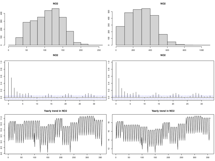
Figure E.1: Various statistical properties of the daily concentrations of NO₂(left) and NO_x (right) measured at Marylebone Road in London between January $2004$ and December $2010$. Top: histogram of raw concentrations. Middle: autocorrelations after square root transform. Bottom: yearly fitted patterns.

The concentration measurements are positive integers and possibly highly skewed, see top panels of Figure E.1. Also, the data exhibit seasonality as well as weekly patterns, the latter particularly visible from the autocorrelations (see middle panels of Figure E.1), and the level of concentrations drops sharply on bank holidays, in line with the behaviour of road traffic. We adopt the square root transform in order to bring the data to light-tailedness without masking any shift in the level greatly. Also, after visual inspection and preliminary research into the relevant literature, we select the period between January 2004 and December 2010 to estimate the seasonal, weekly and bank holiday patterns, which is achieved by regressing the square root transformed time series onto the indicator variables representing their effects. In summary, $19$ parameters including the intercept were estimated from the $2508$ observations, and all three factors (seasonal, daily and bank holiday effects) were deemed significant, with the models fitted to the NO₂ and NO_x concentrations attaining the adjusted $R^{2}$ coefficients of $0.1077$ and $0.1149$, respectively. Bottom panels of Figure E.1 plot the fitted yearly trend, while Figure 2 in the main text plots the residuals, which we analyse for change points in the level.

E.2 Validating the number of change points detected from the NO₂ time series

Table 2 in the main paper shows a considerable variation in the number of detected change points in the NO₂ time series between the competing methods. To run an independent check for the number of change points, we firstly remove the bulk of the serial dependence of the data by fitting the AR($1$) model to it and work with the empirical residuals from this fit. For this, we set the AR coefficient to $0.5$, as suggested by the sample autocorrelation function in Figures E.1 and E.2. In particular, the latter figure confirms that the assumption of weak stationarity on the noise is well-satisfied by the NO₂ time series, with the leading autocorrelations remaining approximately the same across the segments defined by the change points estimated by WCM.gSa.

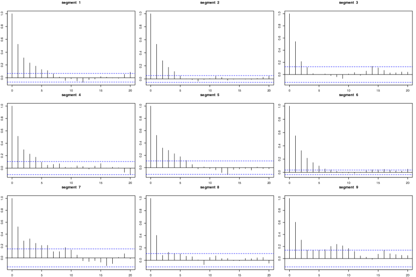
Figure E.2: Autocorrelations at $20$ lags computed from the nine segments defined by the change point estimators returned by WCM.gSa when applied to the de-trended and transformed NO₂ measurements.

On these, we perform change point detection using a method suitable for multiple level-shift detection under serially uncorrelated noise. The method we use is the IDetect technique with the information-criterion-based model selection (Anastasiou and Fryzlewicz,, 2020), as implemented in the R package breakfast (Anastasiou et al.,, 2020). The reason for the selection of this method is that it is possibly the best-performing method of the package overall (as reported in the package vignette available at https://cran.r-project.org/web/packages/breakfast/vignettes/breakfast-vignette.html), and it is independently commended in Fearnhead and Rigaill, (2020) as having very strong performance overall.

The R execution model.ic(sol.idetect(no2.res))$cpts, where no2.res are the residuals obtained as above, returns $7$ change point estimators, a number close to the $8$ obtained by our WCM.gSa method. Out of the $7$ locations estimated by IDetect, there is very good agreement with WCM.gSa for $6$ out of these locations. The exception is the WCM.gSa-estimated change point at 2010-07-25, which IDetect estimates some $800$ days later. However, IDetect also does not estimate the following WCM.gSa-estimated change point at 2018-10-13, which is a possible reason for IDetect to replace these two WCM.gSa-estimated change points by one in between them.

This, in our view, represents very good agreement on the whole, especially given that the two methods are entirely different in nature and worked with different time series on input. This result further enhances our confidence in the output of WCM.gSa for this dataset.

E.3 Hadley Centre central England temperature data analysis

The Hadley Centre central England temperature (HadCET) dataset (Parker et al.,, 1992) contains the mean, maximum and minimum daily and monthly temperatures representative of a roughly triangular area enclosed by Lancashire, London and Bristol, UK.

We analyse the yearly average of the monthly mean, maximum and minimum temperatures up to 2019 for change points using the proposed WCM.gSa methodology. The mean monthly data dates back to 1659, while the maximum and the minimum monthly data begins in 1878; we focus on the period of 1878–2019 ($n=142$) for all three time series. To take into account that the time series are relatively short, we set $p_{\max}=5$ (maximum allowable AR order) for WCM.gSa and the minimum spacing to be $10$ (i.e. no change points occur within $10$ years from one another), while the rest of the parameters are chosen as recommended in Section C; the results are invariant to the choice of the penalty $\xi_{n}\in\{\log^{1.01}(n),\log^{1.1}(n)\}$. Table E.1 reports the change points estimated by WCM.gSa as well as those detected by DepSMUCE and DeCAFS for comparison.

On all three datasets, WCM.gSa and DeCAFS return identical estimators, and the same change points are detected by DepSMUCE (with $\alpha=0.2$). Figure E.3 shows that there appears to be a noticeable change in the persistence of the autocorrelations in the datasets before and after these shifts in the mean are accounted for, which further confirms that the yearly temperatures undergo level shifts over the years. In particular, the second change point detected at 1987/88 coincides with the global regime shift in Earth’s biophysical systems identified around 1987 (Reid et al.,, 2016), which is attributed to anthropogenic warming and a volcanic eruption.

Table E.1: Change points (in year) detected from the yearly average of the mean, maximum and minimum monthly temperatures from 1878 to 2019.

Method	Mean	Maximum	Minimum
WCM.gSa	1892, 1988	1892, 1988	1892, 1987
DepSMUCE(0.05)	1987	1988	1956
DepSMUCE(0.2)	1892, 1988	1988	1892, 1987
DeCAFS	1892, 1988	1892, 1988	1892, 1987

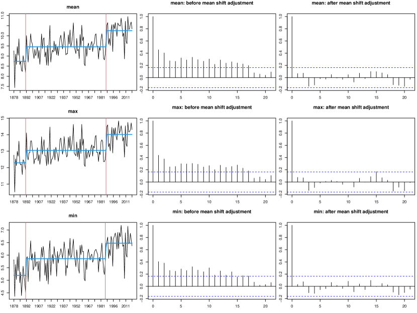
Figure E.3: Left: yearly average of the mean, maximum and minimum monthly temperatures (top to bottom), plotted together with the change points estimated by WCM.gSa (vertical lines) and piecewise constant mean (bold lines). Middle and right: autocorrelation function of the data without and with the time-varying mean adjusted.

Appendix F Proofs

For any square matrix $\mathbf{B}\in\mathbb{R}^{p\times p}$, let $\lambda_{\max}(\mathbf{B})$ and $\lambda_{\min}(\mathbf{B})$ denote the maximum and the minimum eigenvalues of $\mathbf{B}$, respectively, and we define the operator norm $\|\mathbf{B}\|=\sqrt{\lambda_{\max}(\mathbf{B}^{\top}\mathbf{B})}$. Let $\mathbf{1}$ denote a vector of ones, $\mathbf{0}$ a vector of zeros and $\mathbf{I}$ an identity matrix whose dimensions are determined by the context. The projection matrix onto the column space of a given matrix $\mathbf{A}$ is denoted by $\bm{\Pi}_{\mathbf{A}}=\mathbf{A}(\mathbf{A}^{\top}\mathbf{A})^{-1}\mathbf{A}^{\top}$, provided that $\mathbf{A}^{\top}\mathbf{A}$ is invertible. We write $a\vee b=\max(a,b)$ and $a\wedge b=\min(a,b)$.

F.1 Proof of the results in Section 2

Throughout the proofs, we work under the following non-asymptotic bound

$$\max\left(\frac{n^{\varphi}\zeta_{n}^{2}}{\min_{1\leq j\leq q}(f^{\prime}_{j})^{2}\delta_{j}},\frac{1}{\log(\zeta_{n})}\right)\leq\frac{1}{K}$$ (F.1)

for some $K>0$, which holds for all $n\geq n(K)$ for some large enough $n(K)$, which replaces the asymptotic condition in Assumptions 2.2 and (5). The $o$-notation always refers to $K$ in (F.1) being large enough, which in turn follows for large enough $n$. By $\mathcal{F}_{s,k,e}$ and $\mathcal{Z}_{s,k,e}$, we denote the CUSUM statistics defined with $f_{t}$ and $Z_{t}$ replacing $X_{t}$ in (2), respectively.

F.1.1 Preliminaries

Lemma F.1 (Lemma B.1 of Cho and Kirch, (2022)).

For $\max(s,\theta_{j-1})<k<\theta_{j}<\min(e,\theta_{j+1})$, it holds that

$$\mathcal{F}_{s,k,e}=-\sqrt{\frac{(k-s)(e-k)}{e-s}}\left\{\frac{(e-\theta_{j})\,f^{\prime}_{j}}{e-k}+\frac{(e-\theta_{j+1})_{+}\,f^{\prime}_{j+1}}{e-k}+\frac{(\theta_{j-1}-s)_{+}\,f^{\prime}_{j-1}}{k-s}\right\},$$

where $a_{+}=a\cdot\mathbb{I}_{a\geq 0}$. Similarly, for $\max(s,\theta_{j-1})<\theta_{j}\leq k<\min(e,\theta_{j+1})$, it holds that

$$\mathcal{F}_{s,k,e}=-\sqrt{\frac{(k-s)(e-k)}{e-s}}\left\{\frac{(\theta_{j}-s)\,f^{\prime}_{j}}{k-s}+\frac{(e-\theta_{j+1})_{+}\,f^{\prime}_{j+1}}{e-k}+\frac{(\theta_{j-1}-s)_{+}\,f^{\prime}_{j-1}}{k-s}\right\}.$$

Lemma F.2 (Lemma 2.2 of Venkatraman, (1992); Lemma 8 of Wang and Samworth, (2018)).

For some $0\leq s<e\leq n$ with $e-s>1$, let $\Theta\cap[s,e]=\{\theta^{\circ}_{1},\ldots,\theta^{\circ}_{m}\}$ with $m\leq q$, and we adopt the notations $\theta^{\circ}_{0}=s$ and $\theta^{\circ}_{m+1}=e$. If the series $\mathcal{F}_{s,k,e}$ is not constantly zero for $\theta^{\circ}_{j}+1\leq k\leq\theta^{\circ}_{j+1}$ for some $j=0,\ldots,m$, one of the following is true:

1. $j=0$ and $\mathcal{F}_{s,k,e},\,\theta^{\circ}_{j}+1\leq k\leq\theta^{\circ}_{j+1}$ does not change sign and has strictly increasing absolute values,

2. $j=m$ and $\mathcal{F}_{s,k,e},\,\theta^{\circ}_{j}+1\leq k\leq\theta^{\circ}_{j+1}$ does not change sign and has strictly decreasing absolute values,

3. $1\leq j\leq m-1$ and $\mathcal{F}_{s,k,e},\,\theta^{\circ}_{j}+1\leq k\leq\theta^{\circ}_{j+1}$ is strictly monotonic,

4. $1\leq j\leq m-1$ and $\mathcal{F}_{s,k,e},\,\theta^{\circ}_{j}+1\leq k\leq\theta^{\circ}_{j+1}$ does not change sign and its absolute values are strictly decreasing then strictly increasing.

F.1.2 Proof of Theorem 2.1

Throughout the proofs, $C_{0},C_{1},\ldots$ denote some positive constants.

We define the following intervals for each $j=0,\ldots,q_{n}$,

$$I_{L,j}=(\theta_{j-1},\theta_{j}-\lceil\delta_{j}/3\rceil)\quad\text{ and }\quad I_{R,j}=(\theta_{j}+\lceil\delta_{j}/3\rceil,\theta_{j+1}].$$

Let $(s,e)$ denote an interval considered at some iteration of the WBS2 algorithm. By construction, the minimum length of the interval obtained by deterministic sampling is given by $\lfloor(e-s)/\widetilde{K}\rfloor$, where $\widetilde{K}$ satisfies $R_{n}\leq\widetilde{K}(\widetilde{K}+1)/2$. Then, $\mathcal{R}_{s,e}$ drawn by the deterministic sampling contains at least one interval $(\ell_{m(j)},r_{m(j)})$ satisfying $\ell_{m(j)}\in I_{L,j}$ and $r_{m(j)}\in I_{R,j}$ for any $\theta_{j}\in\Theta\cap(s,e)$ (if $\Theta\cap(s,e)$ is not empty), provided that $3\lfloor(e-s)/\widetilde{K}\rfloor\leq 2\min_{1\leq j\leq q}\delta_{j}$. This condition in turn is met under (5). Then, it follows from the proof of Proposition B.1 of Cho and Kirch, (2022) that there exists a permutation $\{\pi(1),\ldots,\pi(q)\}$ of $\{1,\ldots,q\}$ such that on $\mathcal{Z}_{n}$,

$$\max_{1\leq j\leq q}(f^{\prime}_{\pi(j)})^{2}|k_{(j)}-\theta_{\pi(j)}|\leq\rho_{n}=c_{2}\zeta_{n}^{2},\quad\text{and}$$ (F.2)

$$\exp(\mathcal{Y}_{(j)})=\left|\mathcal{X}_{(j)}\right|\geq C_{0}|f^{\prime}_{\pi(j)}|\sqrt{\delta_{\pi(j)}}\geq C_{1}n^{\varphi/2}\zeta_{n}$$ (F.3)

for $j=1,\ldots,q$, by (F.1). From (F.2), the assertion in (i) follows readily. Also consequently, the intervals $(s_{(m)},e_{(m)}),\,m=q+1,\ldots,n-1$ meet one of the followings:

1. $(s_{(m)},e_{(m)})\cap\Theta=\emptyset$, or

2. $(s_{(m)},e_{(m)})\cap\Theta=\{\theta_{j}\}$ and $(f^{\prime}_{j})^{2}\min(\theta_{j}-s_{(m)},e_{(m)}-\theta_{j})\leq\rho_{n}$, or

3. $(s_{(m)},e_{(m)})\cap\Theta=\{\theta_{j},\theta_{j+1}\}$ and $\max\{(f^{\prime}_{j})^{2}(\theta_{j}-s_{(m)}),(f^{\prime}_{j+1})^{2}(e_{(m)}-\theta_{j+1})\}\leq\rho_{n}$,

for some $j=1,\ldots,q$. Under (a), from Assumption 2.1,

$$\exp(\mathcal{Y}_{(m)}) =|\mathcal{Z}_{s_{(m)},k_{(m)},e_{(m)}}|\leq 2\zeta_{n}.$$ (F.4)

Under (b), supposing that $\theta_{j}\leq k_{(m)}$, we obtain

$$\exp(\mathcal{Y}_{(m)}) \leq|\mathcal{F}_{s_{(m)},k_{(m)},e_{(m)}}|+|\mathcal{Z}_{s_{(m)},k_{(m)},e_{(m)}}|$$

$$\leq\sqrt{\frac{(k_{(m)}-s_{(m)})(e_{(m)}-k_{(m)})}{e_{(m)}-s_{(m)}}}\frac{(\theta_{j}-s_{(m)})|d_{j}|}{k_{(m)}-s_{(m)}}+2\zeta_{n}$$

$$\leq\sqrt{d_{j}^{2}\min(\theta_{j}-s_{(m)},e_{(m)}-\theta_{j})}+2\zeta_{n}\leq\sqrt{\rho_{n}}+2\zeta_{n}\leq C_{2}\zeta_{n}$$ (F.5)

by Lemma F.1; the case when $\theta_{j}>k_{(m)}$ is handled analogously. Under (c), we obtain

$$\exp(\mathcal{Y}_{(m)}) \leq\max\left\{|\mathcal{F}_{s_{(m)},\theta_{j},e_{(m)}}|,|\mathcal{F}_{s_{(m)},\theta_{j+1},e_{(m)}}|\right\}+2\zeta_{n}$$

$$\leq\sqrt{d_{j}^{2}(\theta_{j}-s_{(m)})}+\sqrt{d_{j+1}^{2}(e_{(m)}-\theta_{j+1})}+2\zeta_{n}\leq C_{3}\zeta_{n}$$ (F.6)

where the first inequality follows from Lemma F.2 and the second inequality from Lemma F.1. From (F.3) and (F.4)–(F.6), and also that $\mathcal{X}_{(1)}\leq C_{4}\sqrt{n}$ due to $f^{\prime}_{j}=O(1)$, we conclude that

$$\mathcal{Y}_{(m)} =\gamma_{m}\log(n)(1+o(1))=\gamma_{m}\log(n)(1+o(1))+\log(\zeta_{n})\quad\text{for}\quad m=1,\ldots,q,$$

$$\mathcal{Y}_{(m)} \leq\kappa_{m}\log(\zeta_{n})(1+o(1))\quad\text{for}\quad m=q+1,\ldots,P,$$

where $\{\gamma_{m}\}$ and $\{\kappa_{m}\}$ meet the conditions in (ii).

F.2 Proof of the results in Section 3

We adopt the following notations throughout the proof: For a fixed integer $r\geq 1$ and an arbitrary set $\mathcal{A}=\{k_{1},\cdots,k_{m}\}\subset\{1,\ldots,n\}$ satisfying $\min_{0\leq j\leq m}(k_{j+1}-k_{j})\geq r+1$ (with $k_{0}=0$ and $k_{m+1}=n$), we define $\mathbf{X}=\mathbf{X}(\mathcal{A},r)=[\mathbf{L}:\mathbf{R}]$ and $\mathbf{Y}$ as in (14). Also we set $\mathbf{X}_{(j)}=[\mathbf{L}_{(j)}:\mathbf{1}]$ for each $j=0,\ldots,m$, where $\mathbf{L}_{(j)}$ has $\mathbf{x}_{t}=(X_{t},\ldots,X_{t-r+1})^{\top}$, $k_{j}\leq t\leq k_{j+1}-1$ as its rows. Sub-vectors of $\mathbf{Y}$ and $\bm{\varepsilon}$ corresponding to $k_{j}\leq t\leq k_{j+1}-1$ are denoted by $\mathbf{Y}_{(j)}$ and $\bm{\varepsilon}_{(j)}$, respectively. When $r=0$, we have $\mathbf{X}=\mathbf{R}$ and $\mathbf{X}_{(j)}=\mathbf{R}_{(j)}$,

Besides, we denote the (approximate) linear regression representation of (6) with the true change point locations $\theta_{j}$ and AR order $p$ by

$$\mathbf{Y} =\mathbf{L}^{\circ}\bm{\alpha}^{\circ}+\bm{\nu}^{\circ}+\bm{\varepsilon}=\begin{bmatrix}\underbrace{\mathbf{L}^{\circ}}_{n\times p}&\underbrace{\mathbf{R}^{\circ}}_{n\times(q+1)}\end{bmatrix}\;\begin{bmatrix}\bm{\alpha}^{\circ}\\ \bm{\mu}^{\circ}\end{bmatrix}+(\bm{\nu}^{\circ}-\mathbf{R}^{\circ}\bm{\mu}^{\circ})+\bm{\varepsilon},$$ (F.7)

where $\bm{\nu}^{\circ}=((1-a(B))f_{t},\,1\leq t\leq n)^{\top}$. Correspondingly, $\mathbf{X}^{\circ}$ denotes an $n\times(p+q+1)$-matrix with its rows given by

$$\mathbf{x}_{t}=(X_{t-1},\ldots,X_{t-p},\mathbb{I}_{1\leq t\leq\theta_{1}},\ldots,\mathbb{I}_{\theta_{q+1}\leq t\leq n})^{\top}$$

for $1\leq t\leq n$, whereby $\mathbf{X}^{\circ}\equiv\mathbf{X}(\Theta,p)$. When $p=0$, the matrix $\mathbf{L}^{\circ}$ is empty.

F.2.1 Preliminaries

The following results are frequently used throughout the proof.

Proposition F.3.

Suppose that $p\geq 0$ and $r\in\{\max(p,1),\ldots,p_{\max}\}$ with $p_{\max}\geq\max(p,1)$ fixed. Also, let $\mathcal{A}=\{k_{1},\ldots,k_{m}\}$ as an arbitrary subset of $\widehat{\Theta}_{M}$. With such $\mathcal{A}$, define $\mathbf{X}=\mathbf{X}(\mathcal{A},r)=[\mathbf{L}:\mathbf{R}]$ as in (14), and also $\mathbf{X}_{(j)}$, $\mathbf{L}_{(j)}$, $\mathbf{R}_{(j)}$ and $\bm{\varepsilon}_{(j)}$, correspondingly, and let $N_{j}=k_{j+1}-k_{j}$. Then, under Assumption 3.1 (i)–(iii) and Assumption 3.2, we have the followings hold almost surely for all $j=0,\ldots,m$ and $\mathcal{A}\subset\widehat{\Theta}_{M}$:

$$\text{tr}(\mathbf{L}^{\top}\mathbf{L})=O(n),\quad\text{tr}(\mathbf{L}_{(j)}^{\top}\mathbf{L}_{(j)})=O(N_{j}),$$ (F.8)

$$\liminf_{n\to\infty}n^{-1}\lambda_{\min}(\mathbf{L}^{\top}\mathbf{L})>0,\quad\liminf_{n\to\infty}N_{j}^{-1}\lambda_{\min}(\mathbf{L}_{(j)}^{\top}\mathbf{L}_{(j)})>0,$$ (F.9)

$$\text{tr}(\mathbf{X}^{\top}\mathbf{X})=O(n),\quad\liminf_{n\to\infty}n^{-1}\lambda_{\min}(\mathbf{X}^{\top}\mathbf{X})>0,$$

$$\text{tr}(\mathbf{X}_{(j)}^{\top}\mathbf{X}_{(j)})=O(N_{j}),\quad\liminf_{n\to\infty}N_{j}^{-1}\lambda_{\min}(\mathbf{X}_{(j)}^{\top}\mathbf{X}_{(j)})>0,$$ (F.10)

$$(\mathbf{L}^{\top}\mathbf{L})^{-1}\mathbf{L}^{\top}\bm{\varepsilon}=O\left(\sqrt{\frac{\log(n)}{n}}\right),\quad(\mathbf{X}^{\top}\mathbf{X})^{-1}\mathbf{X}^{\top}\bm{\varepsilon}=O\left(\sqrt{\frac{\log(n)}{n}}\right),$$

$$(\mathbf{X}_{(j)}^{\top}\mathbf{X}_{(j)})^{-1}\mathbf{X}_{(j)}^{\top}\bm{\varepsilon}_{(j)}=O\left(\sqrt{\frac{\log(n)}{N_{j}}}\right).$$ (F.11)

Proof.

The results in (F.8)–(F.9) follow from Theorem 3 (ii) of Lai and Wei, (1983) and the finiteness of $\widehat{\Theta}_{M}$. By Corollary 2 of Lai and Wei, 1982a , (F.10) follow from that $\mathsf{tr}(\mathbf{R}^{\top}\mathbf{R})=n$ and $\mathbf{R}_{(j)}^{\top}\mathbf{R}_{(j)}=N_{j}$. By Lemma 1 of Lai and Wei, 1982b , we have

$$\left\|(\mathbf{L}^{\top}\mathbf{L})^{-1/2}\mathbf{L}^{\top}\bm{\varepsilon}\right\| =O\left(\sqrt{\log(\lambda_{\max}(\mathbf{L}^{\top}\mathbf{L}))}\right)=O(\sqrt{\log(n)})\quad\text{a.s.,}$$

$$\left\|(\mathbf{X}^{\top}\mathbf{X})^{-1/2}\mathbf{X}^{\top}\bm{\varepsilon}\right\| =O\left(\sqrt{\log(\lambda_{\max}(\mathbf{X}^{\top}\mathbf{X}))}\right)=O(\sqrt{\log(n)})\quad\text{a.s.,}$$

$$\left\|(\mathbf{X}_{(j)}^{\top}\mathbf{X}_{(j)})^{-1/2}\mathbf{X}_{(j)}^{\top}\bm{\varepsilon}_{(j)}\right\| =O\left(\sqrt{\log(\lambda_{\max}(\mathbf{X}_{(j)}^{\top}\mathbf{X}_{(j)}))}\right)=O(\sqrt{\log(n)})\quad\text{a.s.}$$

which, together with (F.8) and (F.10), leads to (F.11). ∎

Lemma F.4 (Lemma 3.1.2 of Csörgő and Horváth, (1997)).

For any $\mathbf{X}=[\mathbf{L}:\mathbf{R}]$, the OLS estimator $\widehat{\bm{\beta}}=(\mathbf{X}^{\top}\mathbf{X})^{-1}\mathbf{X}^{\top}\mathbf{Y}=(\widehat{\bm{\alpha}}^{\top},\widehat{\bm{\mu}}^{\top})^{\top}$ satisfies $\widehat{\bm{\alpha}}=(\mathbf{L}^{\top}\mathbf{L})^{-1}\mathbf{L}^{\top}(\mathbf{Y}-\mathbf{R}\widehat{\bm{\mu}})$ and $\widehat{\bm{\mu}}=\{\mathbf{R}^{\top}(\mathbf{I}-\bm{\Pi}_{\mathbf{L}})\mathbf{R}\}^{-1}\mathbf{R}^{\top}(\mathbf{I}-\bm{\Pi}_{\mathbf{L}})\mathbf{Y}$.

Lemma F.5.

For some $\mathbf{R}=\mathbf{R}(\mathcal{A})$ constructed with a set $\mathcal{A}=\{k_{1},\ldots,k_{m}\}\subset\{1,\ldots,n\}$ with $k_{1}<\ldots<k_{m}$, we denote by $\mathbf{R}_{-j}$, for any $1\leq j\leq m$, an $n\times m$-matrix formed by merging the $j$-th and the $(j+1)$-th columns of $\mathbf{R}$ via summing them up, while the rest of the columns of $\mathbf{R}$ are unchanged. Then,

$$\|(\mathbf{I}-\bm{\Pi}_{\mathbf{R}_{-j}})\mathbf{U}\|^{2}-\|(\mathbf{I}-\bm{\Pi}_{\mathbf{R}})\mathbf{U}\|^{2}=|\mathcal{C}_{k_{j-1},k_{j},k_{j+1}}(\mathbf{U})|^{2}$$ (F.12)

for any $\mathbf{U}=(U_{1},\ldots,U_{n-(m+1)r})^{\top}$, where

$$\mathcal{C}_{k_{j-1},k_{j},k_{j+1}}(\mathbf{U}):= \sqrt{\frac{(k_{j+1}-k_{j})(k_{j}-k_{j-1})}{k_{j+1}-k_{j-1}}}\times$$

$$\qquad\qquad\left(\frac{1}{k_{j}-k_{j-1}}\sum_{t=k_{j-1}+1}^{k_{j}}U_{t}-\frac{1}{k_{j+1}-k_{j}}\sum_{t=k_{j}+1}^{k_{j+1}}U_{t}\right).$$

Proof.

Denote the $(j+1)$-th column of $\mathbf{R}$ by $\mathbf{R}_{j}$. Then, by simple calculations, we have

$$\|(\mathbf{I}-\bm{\Pi}_{\mathbf{R}})\mathbf{U}\|^{2}=\mathbf{U}^{\top}(\mathbf{I}-\bm{\Pi}_{\mathbf{R}_{-j}})\mathbf{U}-\frac{(\mathbf{U}^{\top}(\mathbf{I}-\bm{\Pi}_{\mathbf{R}_{-j}})\mathbf{R}_{j})^{2}}{\mathbf{R}_{j}^{\top}(\mathbf{I}-\bm{\Pi}_{\mathbf{R}_{-j}})\mathbf{R}_{j}}.$$

Also by construction,

$$\mathbf{R}_{-j}^{\top}\mathbf{R}_{j}=(\underbrace{0,\ldots,0}_{j-1},k_{j+1}-k_{j},0,\ldots,0)^{\top},$$

$$(\mathbf{R}_{-j}^{\top}\mathbf{R}_{-j})^{-1}=\text{diag}\left(\frac{1}{k_{1}},\ldots,\frac{1}{k_{j-1}-k_{j-2}},\frac{1}{k_{j+1}-k_{j-1}},\frac{1}{k_{j+2}-k_{j+1}},\ldots,\frac{1}{n-k_{m}}\right).$$

Hence,

$$[\mathbf{R}_{-j}(\mathbf{R}_{-j}^{\top}\mathbf{R}_{-j})^{-1}\mathbf{R}_{-j}^{\top}\mathbf{R}_{j}]_{i}=\left\{\begin{array}[]{ll}\frac{k_{j+1}-k_{j}}{k_{j+1}-k_{j-1}}&\text{for }k_{j-1}+1\leq i\leq k_{j+1},\\ 0&\text{otherwise,}\end{array}\right.$$

$$[\mathbf{R}_{j}-\mathbf{R}_{-j}(\mathbf{R}_{-j}^{\top}\mathbf{R}_{-j})^{-1}\mathbf{R}_{-j}^{\top}\mathbf{R}_{j}]_{i}=\left\{\begin{array}[]{ll}-\frac{k_{j+1}-k_{j}}{k_{j+1}-k_{j-1}}&\text{for }k_{j-1}+1\leq i\leq k_{j},\\ \frac{k_{j}-k_{j-1}}{k_{j+1}-k_{j-1}}&\text{for }k_{j}+1\leq i\leq k_{j+1},\\ 0&\text{otherwise.}\end{array}\right.$$

Therefore,

$$\mathbf{R}_{j}^{\top}(\mathbf{I}-\bm{\Pi}_{\mathbf{R}_{-j}})\mathbf{R}_{j}=\frac{(k_{j}-k_{j-1})(k_{j+1}-k_{j})}{k_{j+1}-k_{j-1}},$$

$$\mathbf{U}^{\top}(\mathbf{I}-\bm{\Pi}_{\mathbf{R}_{-j}})\mathbf{R}_{j}=\frac{(k_{j}-k_{j-1})(k_{j+1}-k_{j})}{k_{j+1}-k_{j-1}}\left(\frac{1}{k_{j+1}-k_{j}}\sum_{t=k_{j}+1}^{k_{j+1}}U_{t}-\frac{1}{k_{j}-k_{j-1}}\sum_{t=k_{j-1}+1}^{k_{j}}U_{t}\right),$$

which concludes the proof. ∎

F.2.2 Proof of Theorem 3.1

Throughout the proofs, $C_{0},C_{1},\ldots$ denote some positive constants. In what follows, we operate in $\mathcal{E}_{n}\cap\mathcal{M}_{n}$, and all big-$O$ notations imply that they hold a.s. due to Proposition F.3.

We briefly sketch the proof, which proceeds in four steps (i)–(iv) below. We first suppose that Assumption 3.2 holds with $M=1$, and also that $p$ is known. Then, a single iteration of the gSa algorithm in Section A.2 boils down to choosing between $\widehat{\Theta}_{0}=\emptyset$ and $\widehat{\Theta}_{1}$: If $\text{SC}(\{X_{t}\}_{t=1}^{n},\widehat{\Theta}_{1},p)<\text{SC}_{0}(\{X_{t}\}_{t=1}^{n},\widehat{\bm{\alpha}}(p))$, we favour a change point model; if not, we conclude that there is no change point in the data. In (i), when $q=0$, we show that $\mathbf{R}\widehat{\bm{\mu}}\approx\mathbf{1}\mu^{\circ}_{0}\approx\bm{\Pi}_{\mathbf{1}}(\mathbf{Y}-\mathbf{L}\widehat{\bm{\alpha}})$ with $\mu^{\circ}_{0}=(1-\sum_{i=1}^{p}a_{i})f_{0}$ representing the time-invariant overall level, and therefore $\|\mathbf{Y}-\mathbf{X}\widehat{\bm{\beta}}\|^{2}\approx\|(\mathbf{I}-\bm{\Pi}_{\mathbf{1}})(\mathbf{Y}-\mathbf{L}\widehat{\bm{\alpha}})\|^{2}$ which leads to $\text{SC}_{0}(\{X_{t}\}_{t=1}^{n},\widehat{\bm{\alpha}}(p))<\text{SC}(\{X_{t}\}_{t=1}^{n},\widehat{\Theta}_{1},p)$ under Assumption 3.4. In (ii), when $q\geq 1$, we show that

$$\|(\mathbf{I}-\bm{\Pi}_{\mathbf{1}})(\mathbf{Y}-\mathbf{L}\widehat{\bm{\alpha}})\|^{2}-\|\mathbf{Y}-\mathbf{X}\widehat{\bm{\beta}}\|^{2}\geq Cq\min_{1\leq j\leq q}d_{j}^{2}\delta_{j}\gg q\xi_{n}$$

for some fixed constant $C>0$ and thus $\text{SC}_{0}(\{X_{t}\}_{t=1}^{n},\widehat{\bm{\alpha}}(p))>\text{SC}(\{X_{t}\}_{t=1}^{n},\widehat{\Theta}_{1},p)$, provided that $\widehat{\Theta}_{1}$ meets (17). In (iii), we show the consistency of the proposed order selection scheme. For the general case where $M>1$, in (iv), we can repeatedly apply the above arguments for each call of Step 1 of the gSa algorithm: Under Assumption 3.2, when $l>l^{*}$, any $\widehat{\theta}_{l,j}\notin\widehat{\Theta}_{l^{*}}$ are spurious estimators and thus we have the gSa algorithm proceed to examine $\widehat{\Theta}_{l-1}$; when $l=l^{*}$, any $\widehat{\theta}_{l^{*},j}\notin\widehat{\Theta}_{l^{*}-1}$ are detecting those change points undetected in $\widehat{\Theta}_{l^{*}-1}$ and thus the gSa algorithm returns $\widehat{\Theta}_{l^{*}}$.

As outlined above, in the following (i)–(iii), we only consider the case of $M=1$ and consequently drop the subscript ‘$1$’ from $\widehat{\Theta}_{1}$ and $\widehat{\theta}_{1,j}$ where there is no confusion.

For given $\widehat{\Theta}$, recall that $\mathbf{X}=\mathbf{X}(\widehat{\Theta},p)=[\mathbf{L}:\mathbf{R}]$ and $N_{j}=\widehat{\theta}_{j+1}-\widehat{\theta}_{j}$. For $t=\theta_{j}+1,\ldots,\theta_{j}+p$, we have

$$\left|[\bm{\nu}^{\circ}-\mathbf{R}^{\circ}\bm{\mu}^{\circ}]_{t}\right|\leq|d_{j}|\;\max_{1\leq i\leq p}\left|\sum_{i^{\prime}=i}^{p}a_{i^{\prime}}\right|\leq|d_{j}|,$$ (F.13)

for all $1\leq j\leq q$, while $[\bm{\nu}^{\circ}-\mathbf{R}^{\circ}\bm{\mu}^{\circ}]_{t}=0$ elsewhere.

(i) When $q=0$. We first note that

$$\widehat{\bm{\beta}}=(\mathbf{X}^{\top}\mathbf{X})^{-1}\mathbf{X}^{\top}\left(\mathbf{L}\bm{\alpha}^{\circ}+\mu^{\circ}_{0}\mathbf{1}+\bm{\varepsilon}\right)$$

such that by Proposition F.3, we have

$$\left\|\widehat{\bm{\beta}}-\underbrace{\begin{bmatrix}\bm{\alpha}^{\circ}\\ \mu^{\circ}_{0}\mathbf{1}_{\widehat{q}+1}\end{bmatrix}}_{\bm{\beta}^{\circ}(\widehat{q})}\right\|=\left\|(\mathbf{X}^{\top}\mathbf{X})^{-1}\mathbf{X}^{\top}\bm{\varepsilon}\right\|=O\left(\sqrt{\frac{\log(n)}{n}}\right).$$ (F.14)

We decompose the residual sum of squares as

$$\|\mathbf{Y}-\mathbf{X}\widehat{\bm{\beta}}\|^{2}=\|\bm{\varepsilon}\|^{2}+\|\mathbf{X}(\widehat{\bm{\beta}}-\bm{\beta}^{\circ}(\widehat{q}))\|^{2}-2\bm{\varepsilon}^{\top}\mathbf{X}(\widehat{\bm{\beta}}-\bm{\beta}^{\circ}(\widehat{q}))=:\|\bm{\varepsilon}\|^{2}+\mathcal{R}_{11}+\mathcal{R}_{12}.$$

Invoking Proposition F.3 and (F.14),

$$\mathcal{R}_{11}\leq\|\mathbf{X}\|^{2}\;\|\widehat{\bm{\beta}}-\bm{\beta}^{\circ}(\widehat{q})\|^{2}=O\left(\frac{n\log(n)}{n}\right)=O(\log(n))\quad\text{a.s.},$$

and

$$|\mathcal{R}_{12}|\leq\|(\mathbf{X}^{\top}\mathbf{X})^{-1}\mathbf{X}^{\top}\bm{\varepsilon}\|\;\|\mathbf{X}^{\top}\mathbf{X}\|\;\|\widehat{\bm{\beta}}-\bm{\beta}^{\circ}(\widehat{q})\|=O\left(\sqrt{n\log(n)}\cdot\sqrt{\frac{\log(n)}{n}}\right)=O\left(\log(n)\right).$$

Putting together the bounds on $\mathcal{R}_{11}$–$\mathcal{R}_{12}$, we conclude that

$$\|\mathbf{Y}-\mathbf{X}\widehat{\bm{\beta}}\|^{2}=\|\bm{\varepsilon}\|^{2}+O(\log(n)).$$ (F.15)

Next, note that

$$\|(\mathbf{I}-\bm{\Pi}_{\mathbf{1}})(\mathbf{Y}-\mathbf{L}\widehat{\bm{\alpha}})\|^{2} =\|\bm{\varepsilon}\|^{2}-\bm{\varepsilon}^{\top}\bm{\Pi}_{\mathbf{1}}\bm{\varepsilon}+\|(\mathbf{I}-\bm{\Pi}_{\mathbf{1}})\mathbf{L}(\widehat{\bm{\alpha}}-\bm{\alpha}^{\circ})\|^{2}-2\bm{\varepsilon}^{\top}(\mathbf{I}-\bm{\Pi}_{\mathbf{1}})\mathbf{L}(\widehat{\bm{\alpha}}-\bm{\alpha}^{\circ})$$

$$=:\|\bm{\varepsilon}\|^{2}+\mathcal{R}_{21}+\mathcal{R}_{22}+\mathcal{R}_{23}.$$

By the arguments similar to those adopted in Proposition F.3 and Lemma 1 of Lai and Wei, 1982a , we have $|\mathcal{R}_{21}|=O(\log(n))$. Also, by Proposition F.3 and (F.14), $\mathcal{R}_{22}\leq\|\mathbf{L}(\widehat{\bm{\alpha}}-\bm{\alpha}^{\circ})\|^{2}=O(\log(n))$. Next,

$$|\mathcal{R}_{23}|\leq 2\left|\bm{\varepsilon}^{\top}\mathbf{L}(\widehat{\bm{\alpha}}-\bm{\alpha}^{\circ})\right|+2\left|\bm{\varepsilon}^{\top}\bm{\Pi}_{\mathbf{1}}\mathbf{L}(\widehat{\bm{\alpha}}-\bm{\alpha}^{\circ})\right|$$

where the first term is bounded by

$$2\|(\mathbf{L}^{\top}\mathbf{L})^{-1}\mathbf{L}^{\top}\bm{\varepsilon}\|\;\|\mathbf{L}^{\top}\mathbf{L}\|\;\|\widehat{\bm{\alpha}}-\bm{\alpha}^{\circ}\|=O(\log(n))$$

due to Proposition F.3 and Lemma 1 of Lai and Wei, 1982a , and the second term is bounded by the bound on the first term and $\mathcal{R}_{21}$ as $O(\log(n))$. Therefore,

$$\|(\mathbf{I}-\bm{\Pi}_{\mathbf{1}})(\mathbf{Y}-\mathbf{L}\widehat{\bm{\alpha}})\|^{2}=\|\bm{\varepsilon}\|^{2}+O(\log(n)).$$ (F.16)

Combining (F.15) and (F.16) with Assumption 3.1 (ii)–(iii), and noting that $\log(1+x)\leq x$ for all $x\geq 0$,

$$\text{SC}_{0}(\{X_{t}\}_{t=1}^{n},\widehat{\bm{\alpha}}(p))-\text{SC}(\{X_{t}\}_{t=1}^{n},\widehat{\Theta},p)$$

$$=\frac{n}{2}\log\left(1+\frac{\|(\mathbf{I}-\bm{\Pi}_{\mathbf{1}})(\mathbf{Y}-\mathbf{L}\widehat{\bm{\alpha}})\|^{2}-\|\mathbf{Y}-\mathbf{X}\widehat{\bm{\beta}}\|^{2}}{\|\mathbf{Y}-\mathbf{X}\widehat{\bm{\beta}}\|^{2}}\right)-\widehat{q}\xi_{n}=O(\log(n))-\widehat{q}\xi_{n}<0$$

for $n$ large enough, due to Assumption 3.4.

(ii) When $q\geq 1$. Recall that in $\mathcal{M}_{n}$, we have $\widehat{q}=q$. Below we use that by Proposition F.3,

$$\mathsf{tr}(\mathbf{L}^{\top}\mathbf{R})=O(n)\quad\text{and}\quad[\mathbf{L}_{(j)}^{\top}\mathbf{1}]_{i}=O(N_{j})\text{ for }i=1,\ldots,p,\,j=0,\ldots,q,$$ (F.17)

where $\bar{f}=\max_{0\leq j\leq q}|f_{\theta_{j}+1}|$. We first establish the consistency of $\widehat{\bm{\mu}}$ in estimating $\bm{\mu}^{\circ}$.

Applying Lemma F.4, we write

$$\widehat{\bm{\mu}}-\bm{\mu}^{\circ}= (\mathbf{R}^{\top}(\mathbf{I}-\bm{\Pi}_{\mathbf{L}})\mathbf{R})^{-1}\mathbf{R}^{\top}(\mathbf{I}-\bm{\Pi}_{\mathbf{L}})(\bm{\nu}^{\circ}-\mathbf{R}\bm{\mu}^{\circ})+$$

$$(\mathbf{R}^{\top}(\mathbf{I}-\bm{\Pi}_{\mathbf{L}})\mathbf{R})^{-1}\mathbf{R}^{\top}(\mathbf{I}-\bm{\Pi}_{\mathbf{L}})\bm{\varepsilon}=:\mathcal{R}_{31}+\mathcal{R}_{32}.$$

Since $(\mathbf{R}^{\top}(\mathbf{I}-\bm{\Pi}_{\mathbf{L}})\mathbf{R})^{-1}$ is a sub-matrix of $(\mathbf{X}^{\top}\mathbf{X})^{-1}$, we have $\lambda_{\max}((\mathbf{R}^{\top}(\mathbf{I}-\bm{\Pi}_{\mathbf{L}})\mathbf{R})^{-1})\leq(\lambda_{\min}(\mathbf{X}^{\top}\mathbf{X}))^{-1}$ (Horn and Johnson,, 1985, Theorem 4.2.2)) and thus $\liminf_{n\to\infty}n^{-1}\lambda_{\min}(\mathbf{R}^{\top}(\mathbf{I}-\bm{\Pi}_{\mathbf{L}})\mathbf{R})>0$ by Proposition F.3. Also, since $\mathsf{tr}(\mathbf{R}^{\top}(\mathbf{I}-\bm{\Pi}_{\mathbf{L}})\mathbf{R})\leq n$ trivially, we obtain $|\mathcal{R}_{32}|=O\left(\sqrt{\log(n)/n}\right)$ adopting the same arguments used in the proof of (F.11). Next, by (F.13) and since

$$[\mathbf{R}^{\circ}\bm{\mu}^{\circ}-\mathbf{R}\bm{\mu}^{\circ}]_{t}=\left\{\begin{array}[]{ll}d_{j}&\text{for }\theta_{j}+1\leq t\leq\widehat{\theta}_{j},\\ -d_{j}&\text{for }\widehat{\theta}_{j}+1\leq t\leq\theta_{j},\\ \end{array}\right.\text{ for }j=1,\ldots,q$$

while $[\mathbf{R}^{\circ}\bm{\mu}^{\circ}-\mathbf{R}\bm{\mu}^{\circ}]_{t}=0$ otherwise, we obtain

$$\|\bm{\nu}^{\circ}-\mathbf{R}\bm{\mu}^{\circ}\|^{2}\leq 2\|\bm{\nu}^{\circ}-\mathbf{R}^{\circ}\bm{\mu}^{\circ}\|^{2}+2\|\mathbf{R}^{\circ}\bm{\mu}^{\circ}-\mathbf{R}\bm{\mu}^{\circ}\|^{2}\leq 2\sum_{j=1}^{q}d_{j}^{2}\cdot(p+d_{j}^{-2}\rho_{n})=O(q\rho_{n})$$ (F.18)

and therefore $|\mathcal{R}_{31}|^{2}=O\left(q\rho_{n}/n\right)$. Putting together the bounds on $\mathcal{R}_{31}$–$\mathcal{R}_{32}$, we obtain

$$|\widehat{\bm{\mu}}-\bm{\mu}^{\circ}| =O\left(\sqrt{\frac{\log(n)\vee q\rho_{n}}{n}}\right).$$ (F.19)

Also, note that by Lemma F.4,

$$\widehat{\bm{\alpha}}-\bm{\alpha}^{\circ}=(\mathbf{L}^{\top}\mathbf{L})^{-1}\mathbf{L}^{\top}\left\{\bm{\varepsilon}+(\bm{\nu}^{\circ}-\mathbf{R}\bm{\mu}^{\circ})+\mathbf{R}(\bm{\mu}^{\circ}-\widehat{\bm{\mu}})\right\}.$$

Adopting Proposition F.3, (F.17), (F.18) and (F.19), we have

$$\|\widehat{\bm{\alpha}}-\bm{\alpha}^{\circ}\| =O\left(\sqrt{\frac{\log(n)\vee q\rho_{n}}{n}}\right).$$ (F.20)

Next, we consider

$$\|\mathbf{Y}-\mathbf{X}\widehat{\bm{\beta}}\|^{2}= \|\mathbf{L}(\widehat{\bm{\alpha}}-\bm{\alpha}^{\circ})+(\mathbf{R}\widehat{\bm{\mu}}-\bm{\nu}^{\circ})-\bm{\varepsilon}\|^{2}$$

$$= \|\bm{\varepsilon}\|^{2}+\|\mathbf{L}(\widehat{\bm{\alpha}}-\bm{\alpha}^{\circ})\|^{2}+\|\mathbf{R}\widehat{\bm{\mu}}-\bm{\nu}^{\circ}\|^{2}+2(\widehat{\bm{\alpha}}-\bm{\alpha}^{\circ})^{\top}\mathbf{L}^{\top}(\mathbf{R}\widehat{\bm{\mu}}-\bm{\nu}^{\circ})$$

$$-2\bm{\varepsilon}^{\top}\mathbf{L}(\widehat{\bm{\alpha}}-\bm{\alpha}^{\circ})-2\bm{\varepsilon}^{\top}(\mathbf{R}\widehat{\bm{\mu}}-\bm{\nu}^{\circ})=:\|\bm{\varepsilon}\|^{2}+\mathcal{R}_{41}+\mathcal{R}_{42}+\mathcal{R}_{43}+\mathcal{R}_{44}+\mathcal{R}_{45}.$$

By Proposition F.3 and (F.20),

$$\mathcal{R}_{41}=O\left(n\cdot\frac{\log(n)\vee q\rho_{n}}{n}\right)=O\left(\log(n)\vee q\rho_{n}\right).$$

Also, due to (F.18) and (F.19),

$$\mathcal{R}_{42} \leq 2\|\mathbf{R}(\widehat{\bm{\mu}}-\bm{\mu}^{\circ})\|^{2}+2\|\mathbf{R}\bm{\mu}^{\circ}-\bm{\nu}^{\circ}\|^{2}=O\left(\log(n)\vee q\rho_{n}\right)$$ (F.21)

and we also obtain $\mathcal{R}_{43}=O\left(\log(n)\vee q\rho_{n}\right)$. By Proposition F.3 and (F.20),

$$\mathcal{R}_{44} \leq\|(\mathbf{L}^{\top}\mathbf{L})^{-1}\mathbf{L}^{\top}\bm{\varepsilon}\|\;\|\mathbf{L}^{\top}\mathbf{L}\|\;\|\widehat{\bm{\alpha}}-\bm{\alpha}^{\circ}\|=O\left(\sqrt{\log(n)(\log(n)\vee q\rho_{n})}\right)=O\left(\log(n)\vee\sqrt{q}\rho_{n}\right),$$

while with (F.13), (F.19), Assumption 3.1 and Chebyshev’s inequality,

$$|\mathcal{R}_{45}| \leq 2|\bm{\varepsilon}^{\top}\mathbf{R}(\widehat{\bm{\mu}}-\bm{\mu}^{\circ})|+2|\bm{\varepsilon}^{\top}(\mathbf{R}\bm{\mu}^{\circ}-\mathbf{R}^{\circ}\bm{\mu}^{\circ})|+2|\bm{\varepsilon}^{\top}(\mathbf{R}^{\circ}\bm{\mu}^{\circ}-\bm{\nu}^{\circ})|$$

$$=O\left(\sqrt{n\log(n)}\cdot\sqrt{\frac{\log(n)\vee q\rho_{n}}{n}}+\sum_{j=1}^{q}|d_{j}|\cdot\sqrt{d_{j}^{-2}\rho_{n}}\omega_{n}+p\sqrt{\sum_{j=1}^{q}|d_{j}|^{2}}\right)$$

$$=O\left(\log(n)\vee q(\rho_{n}\vee\omega_{n}^{2})\right)$$

on $\mathcal{E}_{n}$. Combining the bounds on $\mathcal{R}_{41}$–$\mathcal{R}_{45}$, we obtain

$$\|\mathbf{Y}-\mathbf{X}\widehat{\bm{\beta}}\|^{2}=\|\bm{\varepsilon}\|^{2}+O\left(\log(n)\vee q\left(\rho_{n}\vee\omega_{n}^{2}\right)\right).$$ (F.22)

Next, note that

$$\|(\mathbf{I}-\bm{\Pi}_{\mathbf{1}})(\mathbf{Y}-\mathbf{L}\widehat{\bm{\alpha}})\|^{2}-\|\mathbf{Y}-\mathbf{X}\widehat{\bm{\beta}}\|^{2}=\left(\|(\mathbf{I}-\bm{\Pi}_{\mathbf{1}})(\mathbf{Y}-\mathbf{L}\widehat{\bm{\alpha}})\|^{2}-\|(\mathbf{I}-\bm{\Pi}_{\mathbf{R}})(\mathbf{Y}-\mathbf{L}\widehat{\bm{\alpha}})\|^{2}\right)$$

$$+\left(\|(\mathbf{I}-\bm{\Pi}_{\mathbf{R}})(\mathbf{Y}-\mathbf{L}\widehat{\bm{\alpha}})\|^{2}-\|\mathbf{Y}-\mathbf{X}\widehat{\bm{\beta}}\|^{2}\right)=:\mathcal{R}_{51}+\mathcal{R}_{52}.$$

Repeatedly invoking Lemma F.5, we have

$$\mathcal{R}_{51}= \|(\mathbf{I}-\bm{\Pi}_{\mathbf{1}})(\mathbf{Y}-\mathbf{L}\widehat{\bm{\alpha}})\|^{2}-\|(\mathbf{I}-\bm{\Pi}_{\mathbf{R}_{-\mathcal{I}_{1}}})(\mathbf{Y}-\mathbf{L}\widehat{\bm{\alpha}})\|^{2}+\sum_{j\in\mathcal{I}_{1}}\left|\mathcal{C}_{\widehat{\theta}_{j-1},\widehat{\theta}_{j},\widehat{\theta}_{j+1}}(\mathbf{Y}-\mathbf{L}\widehat{\bm{\alpha}})\right|^{2}$$

$$\geq \left\lceil\frac{q}{2}\right\rceil\min_{1\leq j\leq q}\left|\mathcal{C}_{\widehat{\theta}_{j-1},\widehat{\theta}_{j},\widehat{\theta}_{j+1}}(\mathbf{Y}-\mathbf{L}\widehat{\bm{\alpha}})\right|^{2}$$

where $\mathbf{R}_{-\mathcal{I}_{1}}$ denotes a matrix constructed by merging the $j$-th and the $(j+1)$-th columns of $\mathbf{R}$ via summing them up for all $j\in\mathcal{I}_{1}$, while the rest of the columns of $\mathbf{R}$ are unchanged, with $\mathcal{I}_{1}$ denoting a subset of $\{1,\ldots,q\}$ consisting of all the odd indices. For notational simplicity, let $\mathcal{C}_{j}(\cdot)=\mathcal{C}_{\widehat{\theta}_{j-1},\widehat{\theta}_{j},\widehat{\theta}_{j+1}}(\cdot)$ where there is no confusion. Note that

$$\mathcal{C}_{j}(\mathbf{Y}-\mathbf{L}\widehat{\bm{\alpha}})=\mathcal{C}_{j}(\mathbf{R}^{\circ}\bm{\mu}^{\circ})+\mathcal{C}_{j}(\bm{\nu}^{\circ}-\mathbf{R}^{\circ}\bm{\mu}^{\circ})+\mathcal{C}_{j}(\bm{\varepsilon})+\mathcal{C}_{j}(\mathbf{L}(\widehat{\bm{\alpha}}-\bm{\alpha}^{\circ})).$$

Without loss of generality, suppose that $\widehat{\theta}_{j}\leq\theta_{j}$. Analogous arguments apply when $\widehat{\theta}_{j}>\theta_{j}$. By Lemma F.1,

$$\mathcal{C}_{j}(\mathbf{R}^{\circ}\bm{\mu}^{\circ})= -\sqrt{\frac{N_{j-1}N_{j}}{N_{j-1}+N_{j}}}\left\{\frac{(N_{j}+\widehat{\theta}_{j}-\theta_{j})d_{j}}{N_{j}}+\frac{(\widehat{\theta}_{j+1}-\theta_{j+1})_{+}d_{j+1}}{N_{j}}\right.$$

$$+\left.\frac{(\theta_{j-1}-\widehat{\theta}_{j-1})_{+}d_{j-1}}{N_{j-1}}\right\}=:\mathcal{R}_{61}+\mathcal{R}_{62}+\mathcal{R}_{63}.$$

Under Assumptions 3.2, 3.3 and 3.4, $\min(N_{j-1},N_{j})^{-1}d_{j}^{2}|\widehat{\theta}_{j}-\theta_{j}|=O(\delta_{j}^{-1}\rho_{n})=o(1)$ (due to $D_{n}^{-1}\rho_{n}\to 0$ as $n\to\infty$) and thus

$$|\mathcal{R}_{61}| =|d_{j}|\sqrt{\frac{N_{j-1}N_{j}}{N_{j-1}+N_{j}}}(1+o(1))\geq|d_{j}|\sqrt{\frac{\min(N_{j-1},N_{j})}{2}}(1+o(1))\geq\sqrt{\frac{d_{j}^{2}\delta_{j}}{2}}(1+o(1)),$$

while

$$|\mathcal{R}_{62}|\leq\frac{d_{j+1}^{2}(\widehat{\theta}_{j+1}-\theta_{j+1})}{\sqrt{d_{j+1}^{2}(\widehat{\theta}_{j+1}-\widehat{\theta}_{j}-p)}}\leq\frac{\rho_{n}}{\sqrt{D_{n}}}(1+o(1))=o(\sqrt{\rho_{n}})$$

and $\mathcal{R}_{63}$ is similarly bounded. Therefore, we conclude

$$\min_{1\leq j\leq q}|\mathcal{C}_{j}(\mathbf{R}^{\circ}\bm{\mu}^{\circ})|\geq\sqrt{\frac{D_{n}}{2}}(1+o(1)).$$ (F.23)

Similarly, by (F.13) and Assumption 3.2, we derive

$$\left|\mathcal{C}_{j}(\bm{\nu}^{\circ}-\mathbf{R}^{\circ}\bm{\mu}^{\circ})\right|\leq p\sqrt{\frac{N_{j-1}N_{j}}{N_{j-1}+N_{j}}}\left\{\frac{|d_{j}|+|d_{j+1}|}{N_{j}}+\frac{|d_{j-1}|}{N_{j-1}}\right\}=o(1).$$ (F.24)

Invoking Assumption 3.1 (iv), it is easily seen that on $\mathcal{E}_{n}$,

$$|\mathcal{C}_{j}(\bm{\varepsilon})|\leq 2\omega_{n}.$$ (F.25)

Finally, by (F.17) and (F.20),

$$\left|\mathcal{C}_{j}(\mathbf{L}(\widehat{\bm{\alpha}}-\bm{\alpha}^{\circ}))\right| =\sqrt{\frac{N_{j-1}N_{j}}{N_{j-1}+N_{j}}}\left|\frac{1}{N_{j-1}}\mathbf{1}^{\top}\mathbf{L}_{(j-1)}(\widehat{\bm{\alpha}}-\bm{\alpha}^{\circ})-\frac{1}{N_{j}}\mathbf{1}^{\top}\mathbf{L}_{(j)}(\widehat{\bm{\alpha}}-\bm{\alpha}^{\circ})\right|$$

$$=O\left(\sqrt{\min(N_{j-1},N_{j})}\cdot\sqrt{\frac{\log(n)\vee q\rho_{n}}{n}}\right)=O\left(\sqrt{\log(n)\vee q\rho_{n}}\right).$$ (F.26)

By (F.23)–(F.26), under Assumption 3.3, there exists some constant $C_{0}>0$ satisfying

$$\mathcal{R}_{51}\geq C_{0}qD_{n}\qquad\text{for $n$ large enough.}$$ (F.27)

Next, we note that

$$\|(\mathbf{I}-\bm{\Pi}_{\mathbf{R}})(\mathbf{Y}-\mathbf{L}\widehat{\bm{\alpha}})\|^{2}=\|\bm{\varepsilon}\|^{2}-\bm{\varepsilon}^{\top}\bm{\Pi}_{\mathbf{R}}\bm{\varepsilon}+\|(\mathbf{I}-\bm{\Pi}_{\mathbf{R}})\mathbf{L}(\widehat{\bm{\alpha}}-\bm{\alpha}^{\circ})\|^{2}+\|(\mathbf{I}-\bm{\Pi}_{\mathbf{R}})\bm{\nu}^{\circ}\|^{2}$$

$$+2(\widehat{\bm{\alpha}}-\bm{\alpha}^{\circ})^{\top}\mathbf{L}^{\top}(\mathbf{I}-\bm{\Pi}_{\mathbf{R}})\bm{\nu}^{\circ}-2\bm{\varepsilon}^{\top}(\mathbf{I}-\bm{\Pi}_{\mathbf{R}})\mathbf{L}(\widehat{\bm{\alpha}}-\bm{\alpha}^{\circ})-2\bm{\varepsilon}^{\top}(\mathbf{I}-\bm{\Pi}_{\mathbf{R}})\bm{\nu}^{\circ}$$

$$=:\|\bm{\varepsilon}\|^{2}-\mathcal{R}_{71}+\mathcal{R}_{72}+\mathcal{R}_{73}+\mathcal{R}_{74}+\mathcal{R}_{75}+\mathcal{R}_{76}.$$

First, by Assumption 3.1 (iv), $\mathcal{R}_{71}=O(\sum_{j=0}^{q}N_{j}\omega_{n}^{2}\cdot N_{j}^{-1})=O(q\omega_{n}^{2})$ on $\mathcal{E}_{n}$. Also, from Proposition F.3 and (F.20), $\mathcal{R}_{72}\leq\|\mathbf{L}(\widehat{\bm{\alpha}}-\bm{\alpha}^{\circ})\|^{2}=O(\log(n)\vee q\rho_{n})$. In addition,

$$\mathcal{R}_{73}\leq 2\|\bm{\nu}^{\circ}-\mathbf{R}\bm{\mu}^{\circ}\|^{2}+2\|\mathbf{R}(\bm{\mu}^{\circ}-(\mathbf{R}^{\top}\mathbf{R})^{-1}\mathbf{R}^{\top}\mathbf{\bm{missing}}\nu^{\circ})\|^{2}$$

where the first term is $O(q\rho_{n})$ as in (F.18). From (F.13) and the definition of $\mathbf{R}$ and $\mathbf{R}^{\circ}$,

$$\bm{\mu}^{\circ}-(\mathbf{R}^{\top}\mathbf{R})^{-1}\mathbf{R}^{\top}\mathbf{R}^{\circ}\bm{\mu}^{\circ} =\begin{bmatrix}\frac{-(\widehat{\theta}_{1}-\theta_{1})_{+}d_{1}}{\widehat{\theta}_{1}}\\ \frac{(\theta_{1}-\widehat{\theta}_{1})_{+}d_{1}-(\widehat{\theta}_{2}-\theta_{2})_{+}d_{2}}{\widehat{\theta}_{2}-\widehat{\theta}_{1}}\\ \vdots\\ \frac{(\theta_{q}-\widehat{\theta}_{q})_{+}d_{q}}{n-\widehat{\theta}_{q}}\end{bmatrix},$$ (F.28)

$$\left|[(\mathbf{R}^{\top}\mathbf{R})^{-1}\mathbf{R}^{\top}(\mathbf{R}^{\circ}\bm{\mu}^{\circ}-\bm{\nu}^{\circ})]_{j}\right| \leq\frac{p(|d_{j-1}|+|d_{j}|)}{\widehat{\theta}_{j}-\widehat{\theta}_{j-1}}$$ (F.29)

(recall that $\widehat{\theta}_{0}=\theta_{0}=0$ and $\widehat{\theta}_{q+1}=\theta_{q+1}=n$) such that by Assumptions 3.2 and 3.3, we obtain

$$\|\mathbf{R}(\bm{\mu}^{\circ}-(\mathbf{R}^{\top}\mathbf{R})^{-1}\mathbf{R}^{\top}\bm{\nu}^{\circ})\|^{2}\leq C_{1}\sum_{j=1}^{q}d_{j}^{2}\cdot\frac{(d_{j}^{-2}\rho_{n})^{2}+p^{2}}{\widehat{\theta}_{j+1}-\widehat{\theta}_{j}}=o(q\rho_{n})$$

for some constant $C_{1}>0$, hence $\mathcal{R}_{73}=O(q\rho_{n})$. The bounds on $\mathcal{R}_{72}$ and $\mathcal{R}_{73}$ imply the $O(\log(n)\vee q\rho_{n})$ bound on $\mathcal{R}_{74}$. Next, since $\lambda_{\max}((\mathbf{L}^{\top}(\mathbf{I}-\bm{\Pi}_{\mathbf{R}})\mathbf{L})^{-1})\leq\lambda_{\min}^{-1}(\mathbf{X}^{\top}\mathbf{X})$, we have

$$|\mathcal{R}_{75}|\leq\|(\mathbf{L}^{\top}(\mathbf{I}-\bm{\Pi}_{\mathbf{R}})\mathbf{L})^{-1}\mathbf{L}^{\top}(\mathbf{I}-\bm{\Pi}_{\mathbf{R}})\bm{\varepsilon}\|\;\|\mathbf{L}^{\top}(\mathbf{I}-\bm{\Pi}_{\mathbf{R}})\mathbf{L}\|\;\|\widehat{\bm{\alpha}}-\bm{\alpha}^{\circ}\|=O\left(\log(n)\vee q\rho_{n}\right)$$

from Lemma 1 of Lai and Wei, 1982a , Proposition F.3 and (F.20). Finally,

$$|\mathcal{R}_{76}|\leq 2|\bm{\varepsilon}^{\top}(\bm{\nu}^{\circ}-\mathbf{R}\bm{\mu}^{\circ})|+2|\bm{\varepsilon}^{\top}\mathbf{R}(\bm{\mu}^{\circ}-(\mathbf{R}^{\top}\mathbf{R})^{-1}\mathbf{R}^{\top}\bm{\nu})|$$

where using the arguments involved in bounding $\mathcal{R}_{45}$, we have the first term bounded by $O(q(\rho_{n}\vee\omega_{n}^{2}))$, while the second term is bounded as

$$O\left(\sum_{j=1}^{q}\sqrt{N_{j}}\omega_{n}\cdot\frac{d_{j}^{-2}\rho_{n}\cdot|d_{j}|}{N_{j}}\right)=O\left(\sum_{j=1}^{q}\frac{\omega_{n}\rho_{n}}{\sqrt{D_{n}}}\right)=O(q\rho_{n}),$$

on $\mathcal{E}_{n}$, recalling (F.28)–(F.29) and by Assumptions 3.1 (iv), 3.2 and 3.3. Therefore, $\mathcal{R}_{76}=O(q(\rho_{n}\vee\omega_{n}^{2}))$. Collecting the bounds on $\mathcal{R}_{71}$–$\mathcal{R}_{76}$, we obtain

$$\|(\mathbf{I}-\bm{\Pi}_{\mathbf{R}})(\mathbf{Y}-\mathbf{L}\widehat{\bm{\alpha}})\|^{2}=\|\bm{\varepsilon}\|^{2}+O\left(\log(n)\vee q(\rho_{n}\vee\omega_{n}^{2})\right).$$ (F.30)

From (F.22), (F.27) and (F.30),

$$\|(\mathbf{I}-\bm{\Pi}_{\mathbf{1}})(\mathbf{Y}-\mathbf{L}^{\circ}\widehat{\bm{\alpha}})\|^{2}-\|\mathbf{Y}-\mathbf{X}\widehat{\bm{\beta}}\|^{2}\geq C_{0}qD_{n}+O\left(\log(n)\vee q(\rho_{n}\vee\omega_{n}^{2})\right).$$ (F.31)

Note that

$$\text{SC}_{0}(\{X_{t}\}_{t=1}^{n},\widehat{\bm{\alpha}}(p))-\text{SC}(\{X_{t}\}_{t=1}^{n},\widehat{\Theta},p)$$

$$=\frac{n}{2}\log\left(1+\frac{\|(\mathbf{I}-\bm{\Pi}_{\mathbf{1}})(\mathbf{Y}-\mathbf{L}^{\circ}\widehat{\bm{\alpha}})\|^{2}-\|\mathbf{Y}-\mathbf{X}\widehat{\bm{\beta}}\|^{2}}{\|\mathbf{Y}-\mathbf{X}\widehat{\bm{\beta}}\|^{2}}\right)-q\xi_{n}=:\frac{n}{2}\log(1+\mathcal{R}_{8})-q\xi_{n}.$$ (F.32)

When $\mathcal{R}_{8}\geq 1$, we have the RHS of (F.32) trivially bounded away from zero by Assumption 3.4. When $\mathcal{R}_{8}<1$, note that for $g(x)=\log(x)/(x-1)$, since $\lim_{x\downarrow 1}g(x)\to 1$ and from its continuity, there exists a constant $C_{2}>0$ such that $\inf_{1\leq x<2}g(x)\geq C_{2}$. Therefore,

$$\frac{n}{2}\log(1+\mathcal{R}_{8})-q\xi_{n}\geq C_{3}qD_{n}+O\left(\log(n)\vee q(\rho_{n}\vee\omega_{n}^{2})\right)-q\xi_{n}>0,$$

invoking Assumption 3.1 (ii)–(iii), (F.22) and (F.31) for some $C_{3}>0$.

(iii) Order selection consistency. Thus far, we have assumed that the AR order $p$ is known. We show next that for $n$ large enough, the order $p$ is consistently estimated by $\widehat{p}$ obtained as in (15). Recall the notation $\widehat{\bm{\beta}}(\widehat{\Theta},r)=(\widehat{\bm{\alpha}}^{\top}(r),\widehat{\bm{\mu}}^{\top}(\widehat{\Theta}))^{\top}$. Firstly, suppose that $r>p$ while $r\leq p_{\max}$. Then, by (F.14) when $q=0$ or by (F.19) and (F.20) when $q\geq 1$ (here, $q$ coincides with the cardinality of $\widehat{\Theta}$), we have

$$\|\widehat{\bm{\alpha}}(r)-\bm{\alpha}^{\circ}(r)\|=O\left(\sqrt{\frac{\log(n)\vee q\rho_{n}}{n}}\right)\quad\text{with}\quad\bm{\alpha}^{\circ}(r)=(\bm{\alpha}^{\circ\top},\underbrace{0,\ldots,0}_{r-p})^{\top}$$

whether there are changes or not, see the steps leading to (F.20). Then, the arguments similar to those adopted in showing (F.15) or (F.22) establish that

$$\|\mathbf{Y}-\mathbf{X}(\widehat{\Theta},r)\widehat{\bm{\beta}}(\widehat{\Theta},r)\|^{2}=\|\bm{\varepsilon}\|^{2}+O\left(\log(n)\vee q(\rho_{n}\vee\omega_{n}^{2})\right)$$

and therefore, we have

$$\text{SC}\left(\{X_{t}\}_{t=1}^{n},\widehat{\Theta},r\right)-\text{SC}\left(\{X_{t}\}_{t=1}^{n},\widehat{\Theta},p\right)$$

$$= -\frac{n}{2}\log\left(1+\frac{\|\mathbf{Y}-\mathbf{X}(\widehat{\Theta},p)\widehat{\bm{\beta}}(\widehat{\Theta},p)\|^{2}-\|\mathbf{Y}-\mathbf{X}(\widehat{\Theta},r)\widehat{\bm{\beta}}(\widehat{\Theta},r)\|^{2}}{\|\mathbf{Y}-\mathbf{X}(\widehat{\Theta},r)\widehat{\bm{\beta}}(\widehat{\Theta},r)\|^{2}}\right)+(r-p)\xi_{n}$$

$$= O\left(\log(n)\vee q(\rho_{n}\vee\omega_{n}^{2})\right)+(r-p)\xi_{n}>0$$

for $n$ large enough, by Assumption 3.4.

Next, consider $r<p$. For notational convenience, let $\bm{\Pi}(r)=\bm{\Pi}_{\mathbf{X}(\widehat{\Theta},r)}$, and the sub-matrix of $\mathbf{X}(\widehat{\Theta},p)$ containing its columns corresponding to the $i$-th lags for $i=r+1,\ldots,p$ by $\mathbf{X}(p|r)$. Then, $[\mathbf{X}(p|r)^{\top}(\mathbf{I}-\bm{\Pi}(r))\mathbf{X}(p|r)]^{-1}$ is a sub-matrix of $(\mathbf{X}(\widehat{\Theta},p)^{\top}\mathbf{X}(\widehat{\Theta},p))^{-1}$ and thus by Theorem 4.2.2 of Horn and Johnson, (1985) and Proposition F.3, we have

$$\lambda_{\max}\left(\mathbf{X}(p|r)^{\top}(\mathbf{I}-\bm{\Pi}(r))\mathbf{X}(p|r)\right)\leq\lambda_{\max}\left(\mathbf{X}(\widehat{\Theta},p)^{\top}\mathbf{X}(\widehat{\Theta},p)\right)$$

$$\qquad\leq\mathsf{tr}\left(\mathbf{X}(\widehat{\Theta},p)^{\top}\mathbf{X}(\widehat{\Theta},p)\right)=O(n)\quad\text{and similarly,}$$ (F.33)

$$\lambda_{\min}\left(\mathbf{X}(p|r)^{\top}(\mathbf{I}-\bm{\Pi}(r))\mathbf{X}(p|r)\right)\geq\lambda_{\min}\left(\mathbf{X}(\widehat{\Theta},p)^{\top}\mathbf{X}(\widehat{\Theta},p)\right)\quad\text{and thus}$$

$$\liminf_{n\to\infty}n^{-1}\lambda_{\min}\left(\mathbf{X}(p|r)^{\top}(\mathbf{I}-\bm{\Pi}(r))\mathbf{X}(p|r)\right)>0.$$ (F.34)

It then follows that

$$\left\|\mathbf{Y}-\mathbf{X}(\widehat{\Theta},r)\widehat{\bm{\beta}}(\widehat{\Theta},r)\right\|^{2}-\left\|\mathbf{Y}-\mathbf{X}(\widehat{\Theta},p)\widehat{\bm{\beta}}(\widehat{\Theta},p)\right\|^{2}$$

$$= \left\|\left[\mathbf{X}(p|r)^{\top}(\mathbf{I}-\bm{\Pi}(r))\mathbf{X}(p|r)\right]^{-1/2}\mathbf{X}(p|r)^{\top}(\mathbf{I}-\bm{\Pi}(r))\mathbf{Y}\right\|^{2}$$

$$\geq \,\lambda_{\min}\left(\mathbf{X}(p|r)^{\top}(\mathbf{I}-\bm{\Pi}(r))\mathbf{X}(p|r)\right)\;\left\|\begin{bmatrix}\alpha^{\circ}_{r+1}\\ \vdots\\ \alpha^{\circ}_{p}\end{bmatrix}\right\|^{2}$$

$$-\left\|\left[\mathbf{X}(p|r)^{\top}(\mathbf{I}-\bm{\Pi}(r))\mathbf{X}(p|r)\right]^{-1/2}\mathbf{X}(p|r)^{\top}(\mathbf{I}-\bm{\Pi}(r))\bm{\varepsilon}\right\|^{2}$$

$$-\left\|\left[\mathbf{X}(p|r)^{\top}(\mathbf{I}-\bm{\Pi}(r))\mathbf{X}(p|r)\right]^{-1/2}\mathbf{X}(p|r)^{\top}(\mathbf{I}-\bm{\Pi}(r))\left(\bm{\nu}^{\circ}-\mathbf{R}(\widehat{\Theta})\bm{\mu}^{\circ}\right)\right\|^{2}$$

$$\geq \,C_{4}n\sum_{i=r+1}^{p}(\alpha^{\circ}_{i})^{2}+O(\log(n))+O(q\rho_{n})$$ (F.35)

with some constant $C_{4}>0$ for $n$ large enough, where the $O(\log(n))$ bound on the RHS of (F.35) is due to (F.33), (F.34) and Lemma 1 of Lai and Wei, 1982a , while the $O(q\rho_{n})$ bound from (F.18), regardless of whether there are change points or not. Therefore, we have

$$\text{SC}\left(\{X_{t}\}_{t=1}^{n},\widehat{\Theta},r\right)-\text{SC}\left(\{X_{t}\}_{t=1}^{n},\widehat{\Theta},p\right)$$

$$= \frac{n}{2}\log\left(1+\frac{\|\mathbf{Y}-\mathbf{X}(\widehat{\Theta},r)\widehat{\bm{\beta}}(\widehat{\Theta},r)\|^{2}-\|\mathbf{Y}-\mathbf{X}(\widehat{\Theta},p)\widehat{\bm{\beta}}(\widehat{\Theta},p)\|^{2}}{\|\mathbf{Y}-\mathbf{X}(\widehat{\Theta},p)\widehat{\bm{\beta}}(\widehat{\Theta},p)\|^{2}}\right)-(p-r)\xi_{n}$$

$$\geq C_{5}n-(p-r)\xi_{n}>0$$

with some constant $C_{5}>0$ for $n$ large enough, by Assumption 3.4, (F.15) and (F.22).

(iv) When $M>1$. The above (i)–(iii) completes the proof in the special case when Assumption 3.2 is met with $M=1$. In the general case where $M>1$, the above proof is readily adapted to prove the claim of the theorem.

1. First, note that for any $l\geq l^{*}$, the intervals examined in Step 1 of the gSa algorithm, $\{\widehat{\theta}_{l-1,u_{v}}+1,\ldots,\widehat{\theta}_{l-1,u_{v}+1}-1\}$, $v=1,\ldots,q^{\prime}_{l}$, correspond to one of the following cases under Assumption 3.2: Null case with no ‘detectable’ change points, i.e. either $\Theta\cap\{\widehat{\theta}_{l-1,u_{v}}+1,\ldots,\widehat{\theta}_{l-1,u_{v}+1}-1\}=\emptyset$, or all $\theta_{j}\in\Theta\cap\{\widehat{\theta}_{l-1,u_{v}}+1,\ldots,\widehat{\theta}_{l-1,u_{v}+1}-1\}$ satisfy $d_{j}^{2}\min(\theta_{j}-\widehat{\theta}_{l-1,u_{v}},\widehat{\theta}_{l-1,u_{v}+1}-\theta_{j})\leq\rho_{n}$, or change point case with $\Theta\cap\{\widehat{\theta}_{l-1,u_{v}}+1,\ldots,\widehat{\theta}_{l-1,u_{v}+1}-1\}\neq\emptyset$ and $d_{j}^{2}\min(\theta_{j}-\widehat{\theta}_{l-1,u_{v}},\widehat{\theta}_{l-1,u_{v}+1}-\theta_{j})\geq D_{n}-\rho_{n}$ for at least one $\theta_{j}\in\Theta\cap\{\widehat{\theta}_{l-1,u_{v}}+1,\ldots,\widehat{\theta}_{l-1,u_{v}+1}-1\}$.

   In fact, when $l=l^{*}$, all $\{\widehat{\theta}_{l^{*}-1,u_{v}}+1,\ldots,\widehat{\theta}_{l^{*}-1,u_{v}+1}-1\}$ for $v=1,\ldots,q^{\prime}_{l^{*}}$, correspond to the change point case, while when $l\geq l^{*}+1$, they all correspond to the null case.

2. In the null case, the set $\mathcal{A}=\widehat{\Theta}_{l}\cap\{\widehat{\theta}_{l-1,u_{v}}+1,\ldots,\widehat{\theta}_{l-1,u_{v}+1}-1\}$ serves the role of the set of spurious estimators, $\widehat{\Theta}$, as in (i) with $|\mathcal{A}|$ serving as $\widehat{q}$. Besides, we account for the possible estimation bias in the boundary points $\widehat{\theta}_{l-1,u_{v}}$ and $\widehat{\theta}_{l-1,u_{v}+1}$ in the case of $q\geq 1$ (while there are no detectable change points within $\{\widehat{\theta}_{l-1,u_{v}}+1,\ldots,\widehat{\theta}_{l-1,u_{v}+1}-1\}$), by replacing the bound (F.14) derived in (i), with (F.19) and (F.20) in (ii). Consequently, (F.15) and (F.16) are written with $O\left(\log(n)\vee\widehat{q}(\rho_{n}\vee\omega_{n}^{2}))\right)$ (see (F.22) and (F.30)), which leads to

   $$\text{SC}_{0}\left(\{X_{t}\}_{t=\widehat{\theta}_{l-1,u_{v}}+1}^{\widehat{\theta}_{l-1,u_{v}+1}},\widehat{\bm{\alpha}}(p)\right)-\text{SC}\left(\{X_{t}\}_{t=\widehat{\theta}_{l-1,u_{v}}+1}^{\widehat{\theta}_{l-1,u_{v}+1}},\mathcal{A},p\right)$$

   $$=O\left(\log(n)\vee|\mathcal{A}|(\rho_{n}\vee\omega_{n}^{2})\right)-|\mathcal{A}|\xi_{n}<0$$

   for $n$ large enough.

3. In the change point case, the arguments under (ii) are applied analogously by regarding $\mathcal{A}$ as $\widehat{\Theta}$ therein, with $|\mathcal{A}|$ equal to the number of detectable change points in $\{\widehat{\theta}_{l-1,u_{v}}+1,\ldots,\widehat{\theta}_{l-1,u_{v}+1}-1\}$ as defined in (a). Then, we obtain

   $$\text{SC}_{0}\left(\{X_{t}\}_{t=\widehat{\theta}_{l-1,u_{v}}+1}^{\widehat{\theta}_{l-1,u_{v}+1}},\widehat{\bm{\alpha}}(p)\right)-\text{SC}\left(\{X_{t}\}_{t=\widehat{\theta}_{l-1,u_{v}}+1}^{\widehat{\theta}_{l-1,u_{v}+1}},\mathcal{A},p\right)$$

   $$\geq C_{3}|\mathcal{A}|D_{n}+O\left(\log(n)\vee|\mathcal{A}|(\rho_{n}\vee\omega_{n}^{2})\right)-|\mathcal{A}|\xi_{n}>0$$

   for $n$ large enough.

4. The proof on order selection consistency in (iii) holds from regardless of whether there are detectable change points in $\{\widehat{\theta}_{l-1,u_{v}}+1,\ldots,\widehat{\theta}_{l-1,u_{v}+1}-1\}$ or not. Thus with (a)–(c) above, the proof is complete.

F.3 Proof of Proposition B.1

For a fixed $j=1,\ldots,q$, we drop the subscript $j$ and write $\check{\theta}=\check{\theta}_{j}$, $\ell=\ell_{j}$, $r=r_{j}$, $\theta=\theta_{j}$, $f^{\prime}=f^{\prime}_{j}$ and $\delta=\delta_{j}$. In what follows, we assume that $\mathcal{X}_{\ell,\check{\theta},r}>0$; otherwise, consider $-X_{t}$ (resp. $-f_{t}$ and $-Z_{t}$) in place of $X_{t}$ ($f_{t}$ and $Z_{t}$). Then, on $\mathcal{Z}_{n}$, we have

$$\max_{\ell<k<r}|\mathcal{Z}_{\ell,k,r}|\leq\max_{\ell<k<r}\left(\sqrt{\frac{r-k}{r-\ell}}+\sqrt{\frac{k-\ell}{r-\ell}}\right)\zeta_{n}=\sqrt{2}\zeta_{n},$$ (F.36)

while by (B.1)–(B.2),

$$|\mathcal{F}_{\ell,\theta,r}|\geq\sqrt{\frac{(f^{\prime})^{2}\delta}{4}}.$$ (F.37)

By Lemma F.2 and (B.2), we have $\mathcal{F}_{\ell,k,r}$ strictly increases, peaks at $k=\theta$ and then decreases in modulus without changing signs. Also by Lemma 7 of Wang and Samworth, (2018), we obtain

$$|\mathcal{F}_{\ell,\theta,r}-\mathcal{F}_{\ell,k,r}|\geq\frac{2}{3\sqrt{6}}\frac{|f^{\prime}|\,|k-\theta|}{\sqrt{\min(\theta-\ell,r-\theta)}}$$ (F.38)

for $|k-\theta|\leq\min(\theta-\ell,r-\theta)/2$. Then, from (F.1) and (F.36)–(F.37),

$$|\mathcal{F}_{\ell,\check{\theta},r}|\geq|\mathcal{F}_{\ell,\theta,r}|-2\max_{\ell<k<r}|\mathcal{Z}_{\ell,k,r}|\geq\sqrt{\frac{(f^{\prime})^{2}\delta}{4}}-2\sqrt{2}\zeta_{n}>\frac{\sqrt{(f^{\prime})^{2}\delta}}{4},$$ (F.39)

which implies that $|\mathcal{Z}_{\ell,\check{\theta},r}|/|\mathcal{F}_{\ell,\check{\theta},r}|=o(1)$ and consequently that $\mathcal{F}_{\ell,\theta,r}>\mathcal{F}_{\ell,\check{\theta},r}>0$ for $n$ large enough. Below, we consider the case where $\check{\theta}\leq\theta$; the case where $\check{\theta}>\theta$ can be handled analogously. We first establish that

$$\theta-\check{\theta}\leq\min(\theta-\ell,r-\theta)/2.$$ (F.40)

If $\theta-\check{\theta}>\min(\theta-\ell,r-\theta)/2\geq\delta/4$ (due to (B.1)), by Lemma F.2 and (F.38), we have

$$\mathcal{F}_{\ell,\theta,r}-\mathcal{F}_{\ell,\check{\theta},r}\geq\frac{1}{3\sqrt{3}}\sqrt{(f^{\prime})^{2}\delta}$$

while $|\mathcal{Z}_{\ell,\theta,r}-\mathcal{Z}_{\ell,\check{\theta},r}|\leq 2\sqrt{2}\zeta_{n}$, thus contradicting that $\mathcal{X}_{\ell,\check{\theta},r}\geq\mathcal{X}_{\ell,\theta,r}$ under (F.1). Next, for some $\widetilde{\rho}_{n}$ satisfying $(f^{\prime})^{-2}\widetilde{\rho}_{n}\leq\delta/4$, we have

$$\mathsf{P}\left({\arg\max}_{\ell<k<r}|\mathcal{X}_{\ell,k,r}|\leq\theta-(f^{\prime})^{-2}\widetilde{\rho}_{n}\right)\leq\mathsf{P}\left(\max_{\theta-\delta/4\leq k\leq\theta-(f^{\prime})^{-2}\widetilde{\rho}_{n}}\mathcal{X}_{\ell,k,r}\geq\mathcal{X}_{\ell,\theta,r}\right)$$

$$\leq\mathsf{P}\left(\max_{\theta-\delta/4\leq k\leq\theta-(f^{\prime})^{-2}\widetilde{\rho}_{n}}(\mathcal{F}_{\ell,k,r}+\mathcal{Z}_{\ell,k,r})^{2}-(\mathcal{F}_{\ell,\theta,r}+\mathcal{Z}_{\ell,\theta,r})^{2}\geq 0\right)$$

$$=\mathsf{P}\left(\max_{\theta-\delta/4\leq k\leq\theta-(f^{\prime})^{-2}\widetilde{\rho}_{n}}-D_{1}(k)D_{2}(k)\,\left(1+\frac{A_{1}(k)}{D_{1}(k)}\right)\left(1+\frac{A_{2}(k)}{D_{2}(k)}\right)\geq 0\right)$$

$$\leq\mathsf{P}\left(\max_{\theta-\delta/4\leq k\leq\theta-(f^{\prime})^{-2}\widetilde{\rho}_{n}}\left|\frac{A_{1}(k)A_{2}(k)}{D_{1}(k)D_{2}(k)}+\frac{A_{1}(k)}{D_{1}(k)}+\frac{A_{2}(k)}{D_{2}(k)}\right|\geq 1\right)$$

$$\leq 2\mathsf{P}\left(\max_{\theta-\delta/4\leq k\leq\theta-(f^{\prime})^{-2}\widetilde{\rho}_{n}}\frac{|A_{1}(k)|}{D_{1}(k)}\geq\frac{1}{3}\right)+2\mathsf{P}\left(\max_{\theta-\delta/4\leq k\leq\theta-(f^{\prime})^{-2}\widetilde{\rho}_{n}}\frac{|A_{2}(k)|}{D_{2}(k)}\geq\frac{1}{3}\right),\quad\text{where}$$

$$D_{1}(k)=\mathcal{F}_{\ell,\theta,r}-\mathcal{F}_{\ell,k,r},\,D_{2}(k)=\mathcal{F}_{\ell,\theta,r}+\mathcal{F}_{\ell,k,r},\,A_{1}(k)=\mathcal{Z}_{\ell,\theta,r}-\mathcal{Z}_{\ell,k,r},\,A_{2}(k)=\mathcal{Z}_{\ell,\theta,r}+\mathcal{Z}_{\ell,k,r}.$$

Note that

$$|A_{1}(k)| \leq\left|\left(\sqrt{\frac{r-\ell}{(\theta-\ell)(r-\theta)}}-\sqrt{\frac{r-\ell}{(k-\ell)(r-k)}}\right)\sum_{t=\ell+1}^{k}(Z_{t}-\bar{Z}_{\ell:r})\right|$$

$$+\sqrt{\frac{r-\ell}{(\theta-\ell)(r-\theta)}}\left|\sum_{t=k+1}^{\theta}(Z_{t}-\bar{Z}_{\ell:r})\right|=:A_{11}(k)+A_{12}(k).$$

For $k<\theta$, we obtain

$$\sqrt{\frac{r-\ell}{(\theta-\ell)(r-\theta)}}-\sqrt{\frac{r-\ell}{(k-\ell)(r-k)}}=\sqrt{\frac{r-\ell}{(\theta-\ell)(r-\theta)}}\left(1-\sqrt{\frac{(\theta-\ell)(r-\theta)}{(k-\ell)(r-k)}}\right)$$

$$\leq \sqrt{\frac{r-\ell}{(\theta-\ell)(r-\theta)}}\left(1-\sqrt{1-\frac{\theta-k}{r-k}}\right)\leq\frac{1}{2}\sqrt{\frac{r-\ell}{(\theta-\ell)(r-\theta)}}\frac{\theta-k}{r-k}$$

and similarly,

$$\sqrt{\frac{r-\ell}{(k-\ell)(r-k)}}-\sqrt{\frac{r-\ell}{(\theta-\ell)(r-\theta)}}\leq\frac{1}{2}\sqrt{\frac{r-\ell}{(k-\ell)(r-k)}}\frac{\theta-k}{\theta-\ell},$$

such that on $\mathcal{Z}_{n}$, due to (B.1) and (F.40),

$$A_{11}(k)\leq\sqrt{\frac{r-\ell}{(\theta-\ell)(r-\theta)}}\frac{2(\theta-k)}{\min(\theta-\ell,r-\theta)}\left(\sqrt{k-\ell}\,\zeta_{n}+\frac{k-\ell}{\sqrt{r-\ell}}\zeta_{n}\right)\leq\frac{4(\theta-k)\zeta_{n}}{\delta}.$$

Also, by (B.1),

$$A_{12}(k)\leq\sqrt{\frac{2}{\delta}}\left(\left|\sum_{t=k+1}^{\theta}Z_{t}\right|+\frac{\theta-k}{\sqrt{r-\ell}}\zeta_{n}\right).$$

Then, by (F.38) and (F.1), there exists some $c_{3}>0$ such that setting $\widetilde{\rho}_{n}=c_{3}(\widetilde{\zeta}_{n})^{2}$, we have

$$\mathsf{P}\left(\max_{\theta-\delta/4\leq k\leq\theta-(f^{\prime})^{-2}\widetilde{\rho}_{n}}\frac{|A_{1}(k)|}{D_{1}(k)}\geq\frac{1}{3},\,\widetilde{\mathcal{Z}}_{n}\right)$$

$$\leq \mathsf{P}\left(\max_{\theta-\delta/4\leq k\leq\theta-(f^{\prime})^{-2}\widetilde{\rho}_{n}}\frac{\sqrt{(f^{\prime})^{-2}\widetilde{\rho}_{n}}}{\theta-k}\sum_{t=k+1}^{\theta}Z_{t}\geq\sqrt{\widetilde{\rho}_{n}}\left(\frac{1}{3}-\frac{(2\sqrt{2}+1)\zeta_{n}}{\sqrt{(f^{\prime})^{2}\delta}}\right),\,\widetilde{\mathcal{Z}}_{n}\right)=0,$$

which holds uniformly over $j=1,\ldots,q$. Next, note that from (F.36),

$$\max_{\theta-\delta/4\leq k\leq\theta-(f^{\prime})^{-2}\widetilde{\rho}_{n}}|A_{2}(k)|\leq 2\sqrt{2}\zeta_{n},$$

while from (F.37),

$$\min_{\theta-\delta/4\leq k\leq\theta-(f^{\prime})^{-2}\widetilde{\rho}_{n}}|D_{2}(k)|\geq\frac{\sqrt{(f^{\prime})^{2}\delta}}{2}$$

and thus

$$\mathsf{P}\left(\max_{\theta-\delta/4\leq k\leq\theta-(f^{\prime})^{-2}\widetilde{\rho}_{n}}\frac{|A_{2}(k)|}{D_{2}(k)}\geq\frac{1}{3},\mathcal{Z}_{n}\right)=0$$

under (F.1), which completes the proof.

Appendix G Assumptions 2.1 and 3.1

In this section, we provide an example that fulfils Assumptions 2.1 and 3.1 (iv) motivated by the Nagaev-type tail probability inequalities derived in Zhang and Wu, (2017) for dependent time series with sub-exponential innovations.

Suppose that $Z_{t}=\sum_{\ell=0}^{\infty}b_{\ell}\varepsilon_{t-\ell}$ where the innovations $\{\varepsilon_{t}\}$ are i.i.d. sub-exponential random variables with $\mathsf{E}(\varepsilon_{t})=0$. Further, we assume that the linear coefficients decay polynomially such that there exists some $\gamma>0$ and $\beta>1$ satisfying $|b_{\ell}|\leq\gamma\ell^{-\beta}$ for all $\ell\geq 1$. With $\nu=1$, the dependence adjusted sub-exponential norm

$$\|Z_{\cdot}\|_{\psi_{\nu},0}=\sup_{m\geq 2}m^{-\nu}\sum_{t=0}^{\infty}\left\{\mathsf{E}\left(\left|Z_{t}-Z_{t,\{0\}}\right|^{m}\right)\right\}^{1/m},$$

is bounded from the above by some fixed constant $C_{1}>0$, where $Z_{t,\{0\}}=\sum_{\ell=0,\,\ell\neq t}^{\infty}b_{\ell}\varepsilon_{t-\ell}+b_{t}\varepsilon_{0}^{\prime}$ with $\varepsilon_{0}^{\prime}$ an independent copy of $\varepsilon_{0}$. Then, by Lemma C.4 of Zhang and Wu, (2017), there exists a fixed constant $C_{2}>0$ such that

$$\mathsf{P}\left(\max_{0\leq s<e\leq n}\frac{1}{\sqrt{e-s}}\left|\sum_{t=s+1}^{e}Z_{t}\right|\geq\zeta_{n}\right)\leq C_{2}n(n+1)\exp\left(-\frac{3\zeta_{n}^{2/3}}{4e\|Z_{\cdot}\|_{\psi_{1},0}}\right),$$

i.e. we can set $\zeta_{n}=C_{3}\log^{3/2}(n)$ with a large enough $C_{3}>0$ (depending only on $\|Z_{\cdot}\|_{\psi_{1},0}$) and have $\mathsf{P}(\mathcal{Z}_{n})\to 1$. Using similar arguments and Bernstein’s inequality (see e.g. Theorem 2.8.1 of Vershynin, (2018)), we have $\mathsf{P}(\mathcal{E}_{n})\to 1$ with $\omega_{n}\asymp\log(n)$.

References

- Air Quality Expert Group, (2004) Air Quality Expert Group (2004). Nitrogen dioxide in the United Kingdom. https://uk-air.defra.gov.uk/library/assets/documents/reports/aqeg/nd-chapter2.pdf. Accessed: 2020-11-04.
- Anastasiou et al., (2020) Anastasiou, A., Chen, Y., Cho, H., and Fryzlewicz, P. (2020). breakfast: Methods for Fast Multiple Change-Point Detection and Estimation. R package version 2.1.
- Anastasiou and Fryzlewicz, (2020) Anastasiou, A. and Fryzlewicz, P. (2020). Detecting multiple generalized change-points by isolating single ones. Preprint.
- Aue and Horváth, (2013) Aue, A. and Horváth, L. (2013). Structural breaks in time series. Journal of Time Series Analysis, 34:1–16.
- Bardet et al., (2012) Bardet, J.-M., Kengne, W., and Wintenberger, O. (2012). Multiple breaks detection in general causal time series using penalized quasi-likelihood. Electronic Journal of Statistics, 6:435–477.
- Berkes et al., (2006) Berkes, I., Horváth, L., Kokoszka, P., Shao, Q.-M., et al. (2006). On discriminating between long-range dependence and changes in mean. The Annals of Statistics, 34:1140–1165.
- Berkes et al., (2014) Berkes, I., Liu, W., and Wu, W. B. (2014). Komlós-Major-Tusnády approximation under dependence. The Annals of Probability, 42:794–817.
- Chakar et al., (2017) Chakar, S., Lebarbier, E., Lévy-Leduc, C., and Robin, S. (2017). A robust approach for estimating change-points in the mean of an AR(1) process. Bernoulli, 23:1408–1447.
- Chan and Yau, (2017) Chan, K. W. and Yau, C. Y. (2017). High-order corrected estimator of asymptotic variance with optimal bandwidth. Scandinavian Journal of Statistics, 44:866–898.
- Chan et al., (2014) Chan, N. H., Yau, C. Y., and Zhang, R.-M. (2014). Group LASSO for structural break time series. Journal of the American Statistical Association, 109:590–599.
- Cho and Fryzlewicz, (2012) Cho, H. and Fryzlewicz, P. (2012). Multiscale and multilevel technique for consistent segmentation of nonstationary time series. Statistica Sinica, 22:207–229.
- Cho and Kirch, (2021) Cho, H. and Kirch, C. (2021). Data segmentation algorithms: Univariate mean change and beyond. Econometrics and Statistics (in press).
- Cho and Kirch, (2022) Cho, H. and Kirch, C. (2022). Two-stage data segmentation permitting multiscale change points, heavy tails and dependence. Annals of the Institute of Statistical Mathematics, 74:653–684.
- Cho and Korkas, (2022) Cho, H. and Korkas, K. K. (2022). High-dimensional GARCH process segmentation with an application to Value-at-Risk. Econometrics and Statistics, 23:187–203.
- Cho et al., (2022) Cho, H., Maeng, H., Eckley, I. A., and Fearnhead, P. (2022). High-dimensional time series segmentation via factor-adjusted vector autoregressive modelling. arXiv preprint arXiv:2204.02724.
- Csörgő and Horváth, (1997) Csörgő, M. and Horváth, L. (1997). Limit Theorems in Change-point Analysis, volume 18. John Wiley & Sons Inc.
- Davis et al., (2006) Davis, R., Lee, T., and Rodriguez-Yam, G. (2006). Structural break estimation for non-stationary time series. Journal of the American Statistical Association, 101:223–239.
- Davis et al., (2008) Davis, R., Lee, T., and Rodriguez-Yam, G. (2008). Break detection for a class of nonlinear time series models. Journal of Time Series Analysis, 29:834–867.
- De la Peña, (1999) De la Peña, V. H. (1999). A general class of exponential inequalities for martingales and ratios. The Annals of Probability, 27:537–564.
- den Haan and Levin, (1997) den Haan, W. J. and Levin, A. T. (1997). A practitioner’s guide to robust covariance matrix estimation. Handbook of Statistics, 15:299 – 342.
- Dette et al., (2020) Dette, H., Schüler, T., and Vetter, M. (2020). Multiscale change point detection for dependent data. Scandinavian Journal of Statistics, 47:1243–1274.
- Doukhan and Neumann, (2007) Doukhan, P. and Neumann, M. H. (2007). Probability and moment inequalities for sums of weakly dependent random variables, with applications. Stochastic Processes and their Applications, 117:878–903.
- Eichinger and Kirch, (2018) Eichinger, B. and Kirch, C. (2018). A MOSUM procedure for the estimation of multiple random change points. Bernoulli, 24:526–564.
- Fang and Siegmund, (2020) Fang, X. and Siegmund, D. (2020). Detection and estimation of local signals. arXiv preprint arXiv:2004.08159.
- Fearnhead and Rigaill, (2020) Fearnhead, P. and Rigaill, G. (2020). Relating and comparing methods for detecting changes in mean. Stat, 9:e291.
- Frick et al., (2014) Frick, K., Munk, A., and Sieling, H. (2014). Multiscale change point inference. Journal of the Royal Statistical Society: Series B (Statistical Methodology), 76:495–580.
- Fryzlewicz, (2014) Fryzlewicz, P. (2014). Wild Binary Segmentation for multiple change-point detection. The Annals of Statistics, 42:2243–2281.
- (28) Fryzlewicz, P. (2020a). Detecting possibly frequent change-points: Wild Binary Segmentation 2 and steepest-drop model selection. Journal of the Korean Statistical Society, pages 1–44.
- (29) Fryzlewicz, P. (2020b). Narrowest Significance Pursuit: inference for multiple change-points in linear models. Preprint.
- Higham et al., (2020) Higham, J., Ramírez, C. A., Green, M., and Morse, A. (2020). UK COVID-19 lockdown: 100 days of air pollution reduction. Air Quality, Atmosphere & Health, pages 1–8.
- Horn and Johnson, (1985) Horn, R. A. and Johnson, C. R. (1985). Matrix Analysis. Cambridge University Press.
- Hušková and Kirch, (2010) Hušková, M. and Kirch, C. (2010). A note on studentized confidence intervals for the change-point. Computational Statistics, 25:269–289.
- Hušková and Slabý, (2001) Hušková, M. and Slabý, A. (2001). Permutation tests for multiple changes. Kybernetika, 37:605–622.
- Kampa and Castanas, (2008) Kampa, M. and Castanas, E. (2008). Human health effects of air pollution. Environmental Pollution, 151:362–367.
- (35) Killick, R., Fearnhead, P., and Eckley, I. A. (2012a). Optimal detection of changepoints with a linear computational cost. Journal of the American Statistical Association, 107:1590–1598.
- (36) Killick, R., Nam, C., Aston, J., and Eckley, I. (2012b). changepoint.info: The changepoint repository. http://changepoint.info/.
- Kirch, (2006) Kirch, C. (2006). Resampling methods for the change analysis of dependent data. PhD thesis, Universität zu Köln.
- Korkas and Fryzlewicz, (2017) Korkas, K. K. and Fryzlewicz, P. (2017). Multiple change-point detection for non-stationary time series using wild binary segmentation. Statistica Sinica, 27:287–311.
- Kovács et al., (2023) Kovács, S., Li, H., Bühlmann, P., and Munk, A. (2023). Seeded binary segmentation: A general methodology for fast and optimal change point detection. Biometrika, 110:249–256.
- Kuelbs and Philipp, (1980) Kuelbs, J. and Philipp, W. (1980). Almost sure invariance principles for partial sums of mixing -valued random variables. The Annals of Probability, pages 1003–1036.
- Kühn, (2001) Kühn, C. (2001). An estimator of the number of change points based on a weak invariance principle. Statistics & Probability Letters, 51:189–196.
- (42) Lai, T. and Wei, C. (1982a). Asymptotic properties of projections with applications to stochastic regression problems. Journal of Multivariate Analysis, 12:346–370.
- (43) Lai, T. and Wei, C. (1982b). Least squares estimates in stochastic regression models with applications to identification and control of dynamic systems. The Annals of Statistics, 10:154–166.
- Lai and Wei, (1983) Lai, T. and Wei, C. (1983). Asymptotic properties of general autoregressive models and strong consistency of least-squares estimates of their parameters. Journal of Multivariate Analysis, 13:1–23.
- Lavielle and Moulines, (2000) Lavielle, M. and Moulines, E. (2000). Least-squares estimation of an unknown number of shifts in a time series. Journal of Time Series Analysis, 21:33–59.
- Lu et al., (2010) Lu, Q., Lund, R., and Lee, T. C. (2010). An MDL approach to the climate segmentation problem. The Annals of Applied Statistics, 4(1):299–319.
- Merlevède et al., (2011) Merlevède, F., Peligrad, M., and Rio, E. (2011). A Bernstein type inequality and moderate deviations for weakly dependent sequences. Probability Theory and Related Fields, 151:435–474.
- Mikosch and Stărică, (2004) Mikosch, T. and Stărică, C. (2004). Nonstationarities in financial time series, the long-range dependence, and the IGARCH effects. The Review of Economics and Statistics, 86:378–390.
- Norwood and Killick, (2018) Norwood, B. and Killick, R. (2018). Long memory and changepoint models: a spectral classification procedure. Statistics and Computing, 28:291–302.
- Parker et al., (1992) Parker, D. E., Legg, T. P., and Folland, C. K. (1992). A new daily central England temperature series, 1772–1991. International Journal of Climatology: A Journal of the Royal Meteorological Society, 12:317–342.
- Peligrad and Utev, (2006) Peligrad, M. and Utev, S. (2006). Invariance principle for stochastic processes with short memory. In High Dimensional Probability, IMS Lecture Notes Monograph Series, volume 51, pages 18–32. Institute of Mathematical Statistics.
- Pešta and Wendler, (2020) Pešta, M. and Wendler, M. (2020). Nuisance parameters free changepoint detection in non-stationary series. TEST, 29(2):379–408.
- Reid et al., (2016) Reid, P. C., Hari, R. E., Beaugrand, G., Livingstone, D. M., Marty, C., Straile, D., Barichivich, J., Goberville, E., Adrian, R., Aono, Y., et al. (2016). Global impacts of the 1980s regime shift. Global change Biology, 22:682–703.
- Robbins et al., (2011) Robbins, M., Gallagher, C., Lund, R., and Aue, A. (2011). Mean shift testing in correlated data. Journal of Time Series Analysis, 32:498–511.
- Romano et al., (2020) Romano, G., Rigaill, G., Runge, V., and Fearnhead, P. (2020). DeCAFS: Detecting Changes in Autocorrelated and Fluctuating Signals. R package version 3.2.3.
- Romano et al., (2022) Romano, G., Rigaill, G., Runge, V., and Fearnhead, P. (2022). Detecting abrupt changes in the presence of local fluctuations and autocorrelated noise. Journal of the American Statistical Association, 117(54):2147–2162.
- Safikhani and Shojaie, (2022) Safikhani, A. and Shojaie, A. (2022). Joint structural break detection and parameter estimation in high-dimensional non-stationary VAR models. Journal of the American Statistical Association, 117(537):251–264.
- Schwarz, (1978) Schwarz, G. (1978). Estimating the dimension of a model. The Annals of Statistics, 6(2):461–464.
- Shao and Zhang, (2010) Shao, X. and Zhang, X. (2010). Testing for change points in time series. Journal of the American Statistical Association, 105:1228–1240.
- Tecuapetla-Gómez and Munk, (2017) Tecuapetla-Gómez, I. and Munk, A. (2017). Autocovariance estimation in regression with a discontinuous signal and -dependent errors: a difference-based approach. Scandinavian Journal of Statistics, 44:346–368.
- Venkatraman, (1992) Venkatraman, E. (1992). Consistency results in multiple change-point problems. Technical Report No. 24, Department of Statistics, Stanford University.
- Vershynin, (2018) Vershynin, R. (2018). High-dimensional Probability: An Introduction with Applications in Data Science, volume 47. Cambridge University Press.
- Verzelen et al., (2020) Verzelen, N., Fromont, M., Lerasle, M., and Reynaud-Bouret, P. (2020). Optimal change-point detection and localization. arXiv preprint arXiv:2010.11470.
- Vladimirova et al., (2020) Vladimirova, M., Girard, S., Nguyen, H., and Arbel, J. (2020). Sub-Weibull distributions: Generalizing sub-Gaussian and sub-Exponential properties to heavier tailed distributions. Stat, 9(1):e318.
- Wang and Samworth, (2018) Wang, T. and Samworth, R. J. (2018). High dimensional change point estimation via sparse projection. Journal of the Royal Statistical Society: Series B (Statistical Methodology), 80:57–83.
- Wu and Zhou, (2020) Wu, W. and Zhou, Z. (2020). Multiscale jump testing and estimation under complex temporal dynamics. arXiv preprint arXiv:1909.06307.
- Yao, (1988) Yao, Y.-C. (1988). Estimating the number of change-points via Schwarz’ criterion. Statistics & Probability Letters, 6:181–189.
- Yau and Davis, (2012) Yau, C. Y. and Davis, R. A. (2012). Likelihood inference for discriminating between long-memory and change-point models. Journal of Time Series Analysis, 33(4):649–664.
- Yau and Zhao, (2016) Yau, C. Y. and Zhao, Z. (2016). Inference for multiple change points in time series via likelihood ratio scan statistics. Journal of the Royal Statistical Society: Series B (Statistical Methodology), 78:895–916.
- Zhang and Wu, (2017) Zhang, D. and Wu, W. B. (2017). Gaussian approximation for high dimensional time series. The Annals of Statistics, 45(5):1895–1919.
- Zhao et al., (2022) Zhao, Z., Jiang, F., and Shao, X. (2022). Segmenting time series via self-normalization. Journal of the Royal Statistical Society: Series B (Statistical Methodology), 84(5):1699–1725.