Heterogeneous excitable systems exhibit Griffiths phases below hybrid phase transitions

Abstract

In $d>2$ dimensional, homogeneous threshold models discontinuous transition occur, but the mean-field solution provides $1/t$ power-law activity decay and other power-laws, thus it is called mixed-order or hybrid type. It has recently been shown that the introduction of quenched disorder rounds the discontinuity and second order phase transition and Griffiths phases appear. Here we provide numerical evidence, that even in case of high graph dimensional hierarchical modular networks a Griffiths phase in the $K=2$ threshold model is present below the hybrid phase transition. This is due to the fragmentation of the activity propagation by modules, which are connected via single links. This provides a widespread mechanism in case of threshold type of heterogeneous systems, modeling the brain or epidemics for the occurrence of dynamical criticality in extended Griffiths phase parameter spaces. We investigate this in synthetic modular networks with and without inhibitory links as well as in the presence of refractory states.

I Introduction

Phase transitions in genuine nonequilibrium systems have often been investigated among reaction-diffusion (RD) type of models exhibiting absorbing states Marro and Dickman (2005); Henkel et al. (2008). In many cases mapping to surface growth, spin systems or stochastic cellular automata have been used. Criticality allows us to define universality classes, defined by the scaling exponents, which have been explored in homogeneous systems Ódor (2004, 2008). In heterogeneous network models the situation is less clear. Hybrid phase transition (HPT) means that at the transition point the order parameter exhibits a jump, in conjunction with critical phenomena related to it. It can mean avalanches of activity at the transition point with power-law (PL) size distribution for example. Such type of transitions have been known for a long time Cardy (1981), for example at tricriticality Janssen et al. (2004); Chan et al. (2015), but had not been the focus of research and the term appeared later. HPT-s have been found in network science in case of $k$-cores  Dorogovtsev et al. (2006), interdependent networks Lee et al. (2016) and multiplexes Baxter et al. (2014).

The ”mixed-order” naming for the same phenomena in statistical physics arouse some years ago Bar and Mukamel (2014) by the exactly soluble one-dimensional Ising model with long range interactions. It is also known to appear in nonequilibrium models, exhibiting transition to absorbing states Juhász and Iglói (2017). Further examples include critical models at extended surface defects Grassberger (2017); Juhász and Iglói (2018) and synchronization Pazó (2005); Gómez-Gardeñes et al. (2011); Coutinho et al. (2013).

Criticality is an ubiquitous phenomenon in nature as systems can benefit many ways from it. As correlations and fluctuations diverge Haimovici et al. (2013) in neural systems working memory and long-connections can be generated spontaneously Johnson S. and Marro (2013) and the sensitivity to external signals is maximal. Furthermore, it has also been shown that information-processing capabilities are optimal near the critical point. Therefore, systems tune themselves close to criticality via self-organization (SOC) Bak et al. (1987); Chialvo (2010), presumably slightly below to avoid blowing over excitation. Besides, if quenched heterogeneity (that is called disorder compared to homogeneous system) is present, rare-region (RR) effects Vojta (2006) and an extended semi-critical region, known as Griffiths Phase (GP) Griffiths (1969) can emerge. RR-s are very slowly relaxing domains, remaining in the opposite phase than the whole system for a long time, causing slow evolution of the order parameter. In the entire GP, which is an extended control parameter region around the critical point, susceptibility diverges and auto-correlations exhibit fat tailed, power-law behavior, resulting in bursty behavior Ódor (2014), frequently observed in nature Karsai et al. (2018). Even in infinite dimensional systems, where mean-field behavior is expected, Griffiths effects Cota et al. (2016) can occur in finite time windows.

It is known that strong disorder can round or smear phase transitions Vojta (2006). According to the arguments by Imry-Ma  Imry and Ma (1975) and Aizenman-Wehr Aizenman and Wehr (1989), first-order transitions do not exist in low-dimensional disordered systems. It has recently been shown Villa Martín et al. (2014, 2015) that this is true in genuinely nonequilibrium systems Marro and Dickman (2005); Ódor (2008).

Experimental and theoretical research provide evidence that the brain operates in a critical state between sustained activity and an inactive phase Beggs and Plenz (2003); Tetzlaff et al. (2010); Hahn et al. (2010); Ribeiro et al. (2010); Haimovici et al. (2013); Ponce-Alvarez et al. (2018); Muñoz (2018). Criticality in general occurs at continuous, second order phase transitions. On the other hand, meta-stability and hysteresis are also common in the brain behavior. They are related to the ability to sustain stimulus-selective persistent activity for working memory Durstewitz et al. (2000). The brain rapidly switches from one state to another in response to stimulus, and it may remain in the same state for a long time after the end of the stimulus. It suggests the existence of a repertoire of meta-stable states. There have been several model describing this  Kaltenbrunner et al. (2007); Scarpetta et al. (2018). It introduces an apparent contradiction, because meta-stability and hysteresis occur in general at first order, discontinuous phase transitions. But the brain can operate at different regimes close to the critical point which can provide the desired advantages for biological systems. Another possible resolution for the above controversy is the operation at a transition of hybrid type. It has also been suggested in a recent theoretical work Buendía et al. (2020).

Threshold type of systems, like the integrate and fire models of the brain Kinouchi and Copelli (2006), are also suggested to describe other phenomena, like power-grids Dobson et al. (2007); Schäffer et al. (2018); Ódor and Hartmann (2018), crack and fracture formation Alava et al. (2006), contagion Unicomb et al. (2018), etc. In these models HPT can emerge naturally, thus the present results can also be relevant.

Heterogeneity effects are very common in nature and result in dynamical criticality in extended GP-s, in case of quasi static quenched disorder approximation Muñoz et al. (2010). This leads to avalanche size and time distributions, with non-universal PL tails. It has been shown within the framework of modular networks Muñoz et al. (2010); Ódor et al. (2015); Cota et al. (2018) and a large human connectome graph Gastner and Ódor (2016). In this study we re-use the hierarchical modular network of  Ódor et al. (2015) and provide numerical evidence that above the GP a HPT emerges. Meta-stable states and hysteresis behavior can also be found, thus this system can oscillate between up and down states, depending on the level of oscillations, without the need of oscillators at the nodes, as in case of the Ginzburg-Landau theory, suggested to model cortical dynamics Di Santo et al. (2018). By extending our model we will show that the proposed mechanism is very general, providing an explanation for the observed wide range of scale-free behavior below the transition point.

II Mean-field approximation

Discrete threshold models can be defined as two-state systems: $x_{i}=0,1$ (inactive, active) at sites $i$, with a conditional activation rule, depending on the sum of activity of neighbors compared to the threshold value $K$:

$$\sum_{j}x_{j}w_{i,j}\geq K\ ,$$ (1)

where $w_{i,j}$ is the weight of the link connecting site $j$ to $i$. In interacting homogeneous systems $w_{i,j}$ is just the adjacency matrix element: $A_{i,j}$, which is 1 if nodes are connected or 0 otherwise. To describe stochasticity this activity creation can be accepted with probability $\lambda$, competing with an activity removal process of probability $\nu$. The mean-field description of the threshold model of $N$ nodes can be obtained in a similar way as in case of RD systems Ódor (2003). That work is defined on the lattice, but we can apply it for other graphs. In Ódor (2003) it was shown that discontinuous jump occurs in mean-field models of the $n>m$ RD systems, in which $n$ neighboring particles are needed for creation and $m$ neighbors for removal. Here we don’t have diffusion and particles, but the activity can be considered as site occupancy and we can map the threshold model with $K=2$ to an RD system with $n=2$ active neighbors necessary for creation and $m=1$ for spontaneous removal. In the presence of inhibitions $n>2$ is needed for creation at nodes with negatively weighted incoming links which increases the inactive phase.

In the mean-field approximation the probability of site activity is $\rho$, and two active neighboring sites can occur in a $(N-1)(N-2)/2$ way thus the creation rate in case of a global acceptance probability $\Lambda$ is

$$\frac{1}{2}(N-1)(N-2)\Lambda\rho^{2}(1-\rho)\ .$$ (2)

Let us call : $\Lambda(N-1)(N-2)/2=\lambda$. For a full graph of $N$ nodes we can setup the rate equation

$$\frac{d\rho}{dt}=\lambda\rho^{2}(1-\rho)-\nu\rho\ ,$$ (3)

which in the $N\to\infty$ limit provides $\lambda_{c}=0$, but for finite graphs $\lambda_{c}>0$. In the steady state we have

$$\lambda\rho^{2}(1-\rho)-\nu\rho=0\ .$$ (4)

By imposing the condition

$$\nu=1-\lambda\ ,$$ (5)

we obtain

$$\lambda\rho(1-\rho)-(1-\lambda)=0\ ,$$ (6)

which can be solved as

$$\rho=\frac{\lambda\pm\sqrt{\lambda^{2}-4\lambda(1-\lambda)}}{2\lambda}\ .$$ (7)

The solution is real and positive if

$$\lambda>\lambda_{c}=4/5\ ,$$ (8)

providing a threshold within a system of size $N$

$$\Lambda_{c}=\frac{8}{5(N-1)(N-2)}$$ (9)

and an order parameter for $\Lambda\to\Lambda_{c}^{+}$

$$\rho_{c}=1/2\ .$$ (10)

It is important to realize that in the $N\to\infty$ limit $\Lambda_{c}\to 0$, thus there is no inactive phase in the thermodynamic limit. But as real systems are always finite sized, we can observe this hybrid phase transition in them even in the mean-field limit. Similar phenomenon has recently been reported in contagion models Choi et al. (2018). Furthermore, in case of the presence of inhibitory couplings the HPT at finite transition rate may survive the $N\to\infty$ limit in high dimensional systems.

At this transition point we can determine how the density approaches $\rho_{c}$:

$$\rho(t)-\rho_{c}\sim t^{-1}\ .$$ (11)

Thus here we find PL dynamical behavior even though the transition is discontinuous, as in other known hybrid or mixed order transitions. For $\lambda<\lambda_{c}$ we have $\rho=0$ stable solution and exponentially decaying activity. Right above the transition the steady state density vanishes with a square-root singularity as in case of k-core Dorogovtsev et al. (2006) or multiplex percolation hybrid transitions Baxter et al. (2014):

$$(\rho-\rho_{c})\propto(\lambda-\lambda_{c})^{1/2}\ ,$$ (12)

but unlike the contact process Harris (1974) near multiple junctions Juhász and Iglói (2017), or the Kuramoto model with uniform frequency distribution Pazó (2005), which thus belong to another hybrid universality class. In the following sections we investigate what happens to this HPT if we implement the threshold model on a hierarchical modular network (HMN).

III Threshold model on hierarchical modular networks

In this section we describe the HMN models we use for the simulations. It is important to note that we believe that hierarchy is not relevant, but that modularity is what enhances RR effects as in case of the study Cota et al. (2018). The models are motivated by brain networks originated from Kaiser and Hilgetag, who performed numerical studies to investigate the effects of different topologies on the activity spreading Kaiser and Hilgetag (2010). Their hierarchical model reflects general features of brain connectivity at large and mesoscopic scales, where the nodes were intended to represent cortical columns instead of individual neurons. The connections between them were modeled excitatory, since there appears to be no long-distance, inhibitory connections within the cerebral cortex Latham and S. (2004).

The network was generated beginning with the highest level and adding modules to the next lower level with random connectivity within modules. Kaiser and Hilgetag explored hierarchical networks with different numbers of hierarchical levels and numbers of sub-modules at each level. The total, average node degree was set to a fixed value, motivated by comparative experimental studies. However, they investigated different topologies by varying the edge density across the levels. All the tested HMN-s were small-world type, i.e. exhibited infinite topological dimensions.

The spreading model they investigated was a two-state threshold model, in which nodes became activated with probability $\lambda$, when at least $K$ of their directly connected node neighbors were active at the same time or spontaneously deactivated, with probability $\nu$. Note that this model is very similar to RD models known in statistical physics Ódor (2004, 2008), with a synchronous cellular automaton (SCA) update. Without loss of generality this algorithm produces faster dynamical scaling results for threshold models than those with random sequential updates.

In this paper we investigate versions of HMN-s, which possess increasing edge density from top to bottom levels. Clearly, such topologies can be expected to be more suitable for activity localization and for RR effects.

Figure 1: Plot of the adjacency matrix of an $N=1024$ sized sample of the HMN2d graph used. Black dots denote connections between nodes $i$ and $j$. The 4-level structure is clearly visible by the blocks along the diagonal, additional long-range edges are scattered points around it.

One can also make a correspondence with the spatially embedded networks Barthelemy (2018). These networks have long links, with algebraically decaying probabilities in the Euclidean distance $R$ as

$$p(R)\sim R^{-s}.$$ (13)

We added random long links by level-to-level from top to bottom, similar to in Ódor et al. (2015). The levels $l=0,1,...,l_{max}$ are numbered from bottom to top. The size of domains, i.e the number of nodes in a level, grows as $N_{l}=4^{l+1}$ in the case of the $4$-module construction, related to a tiling of the 2d base lattice, due to the rough distance level relation:

$$p_{l}=b(\frac{1}{2^{s}})^{l}.$$ (14)

Here $b$ is related to the average degree $\langle k\rangle$ of nodes , which was prescribed to be $\langle k\rangle=12$ for this construction.

We connected nodes in a hierarchical modular way as if they were embedded in a regular two-dimensional lattice (HMN2d) as shown by the adjacency matrix on Fig. 1, similarly as in Ódor et al. (2015). The $4$ nodes of the level $l=0$ were fully connected. The single connectedness of the networks is guaranteed by additional linking of these $4$-node modules, by two edges to the subsequent ones: the first and the last nodes of module (i) to the first node of module (i+1). Accidental multiple connections were removed and self-connections were not allowed. Note that the single connectedness at low level does not result in stable steady states in case of the threshold value $K=2$.

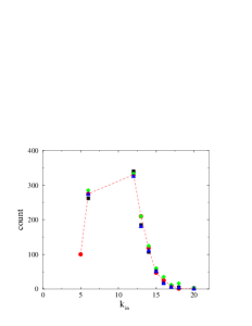
The in-degree distribution of 4 randomly selected graphs with $N=4096$ nodes can be seen on Fig. 2. The lowest in-degree is always $k^{in}_{i}\geq 5$.

Figure 2: In-degree distribution of 4 randomly selected $l=5$ HMN2d graphs.

The modularity quotient of the networks is high: $Q>0.9$, defined by

$$Q=\frac{1}{N\langle{k}\rangle}\sum\limits_{ij}\left(A_{ij}-\frac{k_{i}k_{j}}{N\langle{k}\rangle}\right)\delta(g_{i},g_{j}),$$ (15)

where $A_{ij}$ is the adjacency matrix and $\delta(i,j)$ is the Kronecker delta function. The Watts-Strogatz clustering coefficient Watts and Strogatz (1998) of a network of $N$ nodes is

$$C=\frac{1}{N}\sum_{i}2n_{i}/k_{i}(k_{i}-1)\ ,$$ (16)

where $n_{i}$ denotes the number of direct edges interconnecting the $k_{i}$ nearest neighbors of node $i$. $C=0.295$ is about $10$ times higher than that of a random network of same size $C_{r}=0.0029$, defined by $C_{r}=\langle k\rangle/N$. The average shortest path length is defined as

$$L=\frac{1}{N(N-1)}\sum_{j\neq i}d(i,j)\ ,$$ (17)

where $d(i,j)$ is the graph distance between vertices $i$ and $j$. In case of this typical network $L=6.74$, about twice larger than that of the random network of same size: $L_{r}=3.615$, following from the formula Fronczak et al. (2004):

$$L_{r}=\frac{\ln(N)-0.5772}{\ln\langle k\rangle}+1/2\ .$$ (18)

So this is a small-world network, according to the definition of the coefficient Humphries and Gurney (2008):

$$\sigma=\frac{C/C_{r}}{L/L_{r}}\ ,$$ (19)

because $\sigma=5.363$ is much larger than unity.

We estimated the effective topological dimension using the breadth-first search (BFS) algorithm: $d=4.18(5)$, defined by $N(r)\sim r^{d}$, where we counted the number of nodes $N(r)$ with chemical distance $r$ or less from the seeds and calculated averages over the trials. Note, that this is just an estimate for the finite sized graph, because we know that $d\to\infty$ is expected for $s=3$. It renders this model into the mean-field region, because for threshold models the upper-critical dimension is $d_{c}\leq 4$. Still, due to the heterogeneous structure, we find very non-trivial dynamical GP scaling behavior as will be shown in the following sections.

IV Dynamical simulations

Time dependent simulations were performed for single active seed initial conditions. It means that a pair of nodes is activated at neighboring sites: $x_{i}=x_{i+1}=1$, in an otherwise fully inactive system. It can trigger an avalanche, a standard technique in statistical physics to investigate critical initial slip Henkel et al. (2008). We measured the spatio-temporal size $s=\sum_{i=1}^{N}\sum_{t=1}^{T}x_{i}$ and the duration of the avalanches ($T$) for tens of thousands of random initial conditions: both initial sites and initial graph configurations. The graphs we investigated had $l=4,5,6,7$ levels, containing $N=1024,4096,16384,65536$ nodes, respectively. The average node degree was $\langle k\rangle\simeq 12$, after the low level linking and the removal of accidental multiple edges. The ratio of short and long links was $\simeq 0.6$.

We have set $\nu=1-\lambda$ and updated the sites at discrete time steps, i.e. set the state variables $x^{\prime}(i)=1$ if it was inactive $x(i)=0$ and the sum of active neighbors $\sum_{j}x(j)$ exceeded $K=2$ with probability $\lambda$ or to $x^{\prime}(i)=0$ with probability $1-\lambda$ if it was active $x(i)=1$. Following a full sweep of sites we wrote $x(i)=x^{\prime}(i)$ for all nodes, corresponding to one Monte Carlo step (MCs), throughout the study we measure time in MCs units. We have measured the density of active nodes $\rho(t)=1/N\sum_{i=1}^{N}x_{i}$.

IV.1 Excitatory model

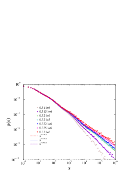
The simulations were run for $T=10^{7}$ MCs, or until the system goes to a fully inactive state, corresponding to the end of the avalanche. We computed the probability density functions of avalanche sizes $p(s)$ and final survival time distributions $p(t)$. We repeated these simulations for different $\lambda$ branching rates, by increasing its value. As Fig. 3 shows we don’t see exponential decays as should be in the inactive phase of a mean-field model. Instead, there are PL-like tails for $\lambda>0.31$, modulated slightly by oscillations, which is a well known phenomenon when discrete spatial periodicity is present, here the size of the modules. The slopes of the PL tails vary from $\tau=2.02$ to $\tau=1.39$ as we increase $\lambda$ from $0.315$ to $0.33$.

Figure 3: Avalanche size distributions at different $\lambda$ branching rates, denoted by the symbols, in the presence of excitatory links in the HMN2d with $l=5,6$ levels. From top to bottom curves: $\lambda=$ 0.33, 0.325, 0.322, 0.32 ($l=5$ cyan and $l=6$ green), 0.315, 0.31. Dashed lines show PL fits for the tails: $s>1000$ at $\lambda=$ 0.315, 0.322, 0.33.

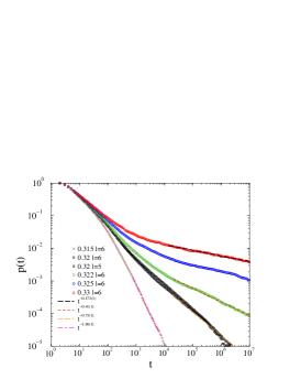
Non-universal PL tails are more clearly visible on the avalanche survival time distributions plotted on the graph, shown on Fig. 4. Here we can observe a greater variation as moving from $\lambda=0.315$ with $\delta=1.80(1)$ to $\lambda=0.33$ with $\delta=0.172(1)$. The avalanche duration distributions can be deduced from these curves as the time integral, thus $\delta$ is related to the duration exponent of $P(t)\propto t^{-\tau_{t}}$ as

$$\tau_{t}=1+\delta\ .$$ (20)

These non-universal PL-s suggest that Griffiths effects are present, as reported in  Ódor et al. (2015) for this model at different parameters. By repeating the simulations at different sizes: $l=5,6$ the distribution curves do not change within error margin, and this size invariance implies the presence of real GP-s.

Figure 4: Survival probability of the activity at different branching rates in the $K=2$ threshold model with excitatory links. From top to bottom curves: $\lambda=$ 0.33, 0.325, 0.322, 0.32 ($l=5$ and $l=6$), 0.315. Dashed lines show PL fits for the tails: $s>10^{4}$ at $\lambda=$ 0.315, 0.322, 0.33.

The seminal experiments by Beggs and Plenz Beggs and Plenz (2003) reported neuronal avalanches with size ($s$) dependence, defined as either the number of electrodes with supra-threshold activity or the sum of the potentials, according to a power law, $p(s)\propto s^{-1.5}$. For the duration distribution of such events $P(t)\propto t^{-2}$, PL tails were observed. These exponents are in agreement with the mean-field (MF) exponents of the Directed Percolation (DP) criticality: $\tau=3/2$, $\tau_{t}=2$ see Ódor (2004). Mean-field exponents are expected to occur if the fluctuation effects are weak, when the system dimension is above the upper critical dimension $d_{c}$.

On the other hand, Palva et al. Palva et al. (2013) have found that source-reconstructed M/EEG data exhibit robust power-law, long-range time correlations and scale-invariant avalanches with a broad range of exponents: $1<\tau<1.6$ and $1.5<\tau_{t}<2.4$. These broad range exponent results have also been found in a recent cortical electrode experiment study on rodents Fontenele et al. (2019). An obvious explanation for this wide spread of critical exponents can be heterogeneity, which in the GP causes non-universal dynamical exponents Moretti and Muñoz (2013); Ódor et al. (2015); Ódor (2016, 2019).

IV.2 Inhibitory model

Although inhibitory links are not expected at long range links of the brain Latham and S. (2004), we believe that our synthetic model may describe smaller cortical scales as well. Besides, inhibitory mechanisms can occur in other phenomena with threshold dynamics. In case of power-grids, for example, feedback is applied to prevent catastrophic blackout avalanches, or in models of social/epidemic contagion, nodes with inhibitory properties may also exist. For simplicity we modeled the inhibitions by the introduction of links with negative weight contribution ($w_{i,j}$) in the threshold comparison rule given by Eq. 1, although we think our results are easily transferred to the case of inhibitory nodes. As in Ódor (2016, 2019), we randomly flipped the sign of $20\%$ of the edges after the generation of the network.

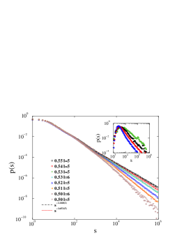
The same analysis resulted in similar behavior as for the excitatory case. One can see $p(s)$ distributions with non-universal PL-s ranging from $\lambda=0.5$ with $\tau=1.651(1)$ to $\lambda=0.55$ with $\tau=1.168(1)$ (Fig. 5). Finite size dependence is not visible by changing the size from $N=4096$ to $N=16384$.

Usually it is believed that overlapping avalanches distort the scaling behavior. From the point of view of statistical physics, this would contradict universal asymptotic scaling behavior. Indeed we can see the same cumulative $p(s)$ distribution tails even in case of starting the system from half filled active state as shown on the inset of Fig. 5. The only difference is that the tails are shifted to larger $s$ values following an initial growth, which might not be observed in case of short time measurements.

Figure 5: Avalanche size distributions at different $\lambda$ branching rates, denoted by the symbols, in the presence of inhibitory links in HMN2d with $l=5,6$ levels. From top to bottom curves: $\lambda=$0.55, 0.54, 0.53 ($l=5$ green and $l=6$ cyan), 0.52, 0.51, 0.50 ($l=5$ triangle and $l=6$ diamond). Dashed lines show power-law fits for the tails of $\lambda=0.5,0.6$ cases, i.e. for $t>1000$. Inset: overlapping avalanches case for half filled initial condition at: $\lambda=0.51,0.515,0.52,0.525$ (bottom to top symbols).

The $p(t)$ decays show GP behavior from $\lambda=0.505$ with $\delta=1.10(3)$ to $\lambda=0.52$ with $\delta=0.70(3)$ (Fig. 6). These values do not correspond to the ends of the GP, we did not aim to determine them precisely as the exponents are non-universal. Furthermore, as we will show in Sect. V the determination of the upper limit of the GP, corresponding to the critical decay is almost impossible by numerical simulations.

Figure 6: Survival probability of the activity at different branching rates and $\nu=1-\lambda$ for the $K=2$ threshold model with levels: $l=5,6$ for the case with $20\%$ of inhibitory links. From bottom to top symbols: $\lambda=$ 0.5, 0.505, 0.510, 0.515, 0.520 ($l=5$ purple cross and $l=6$ blue circle), 0.525 ($l=5$ brown cross and $l=6$ brown circle).

Again the $\tau$ and the $\tau_{t}=1+\delta$ values lie within the range obtained by experiments.

IV.3 Inhibitory-refractory model

Finally, we extended the inhibitory case study with the possibility of refractory states. Refractorieness means that, following an activation, nodes cannot fall back immediately to inactive state on the next update, instead they stay for time $\Delta t$ in a refractory state. Thus they cannot be reactivated by the neighbors they excited. This refractoriness is generic in excitable systems and has been used in most of the neural studies Haimovici et al. (2013); Moosavi et al. (2017); Zarepour et al. (2019). One of the consequences of refractoriness is to induce oscillatory dynamics if $\Delta t$ is large enough and the spreading properties resemble to annular growth, corresponding to Dynamical Isotropic Percolation (DIP) Ódor (2008). However, real DIP occurs if re-activation is not possible, i.e. in the limit $\Delta t\to\infty$, and in high dimension the avalanche scaling exponents of DIP are the same as those of DP Muñoz et al. (1999); Ódor (2008). Thus analytic studies or simulations in high dimensions do not show differences. In the extensive GP simulations we used $\Delta t=1$, but on the inset of Fig. 7 we show oscillatory activity behavior of a single run for $\Delta t=10$, $\lambda=0.8$ and $l=6$.

In Ódor (2019) the GP behavior of inhibitory-refractory threshold model was investigated on a large human connectome graph numerically. Non-universal $p(s)$ decays were reported with $1.4<\tau<1.91$. Here we can see this in the range $\lambda=0.39$ with $\tau=1.96(2)$, to $\lambda=0.43$ with $\tau=1.39(1)$.

Figure 7: Avalanche size distributions at different $\lambda$ branching rates, denoted by the symbols, in case of the refractory model, in the presence of inhibitory links in HMN2d-s with $l=5,6$ levels. From bottom to top symbols: $\lambda=$ 0.39, 0.40 ($l=5$ left triangle and $l=6$ up triangle), 0.41, 0.42, 0.43. Dashed lines are PL fits for the tails of $\lambda=0.5,0.6$ cases for $t>1000$. The inset shows the oscillatory behavior of $\rho(t)$ of a single run for $\Delta t=10$.

The avalanche survival probabilities (see Fig. 8), exhibit PL decay from $\lambda=0.40$ with $\delta=0.92(1)$, to $\lambda=0.43$ with $\delta=0.39(1)$, so the duration exponent varies continuously: $1.39(1)\leq\tau_{t}\leq 1.92(1)$.

Figure 8: Survival probability of the activity at different branching rates $\lambda$ for the levels: $l=5,6$, in case of the inhibitory-refractory model. From bottom to top symbols: $\lambda=$0.40, 0.41 ($l=5$ and $l=6$), 0.42 ($l=5$ light green and $l=6$ dark green), 0.43. Dashed lines show PL fits for $t>1000$ for the $\lambda=$ 0.4, 0.41, 0.43 cases. Inset: $\rho(t)$ at $\lambda=1$, $l=7$ averaged over $10^{5}$ realizations. Blue boxes: excitatory, red diamonds: inhibitory. Black bullets: BFS $\rho(r)$ results. Dashed lines are PL fits for the initial regions: $1\leq t<10$) resulting in effective dimensions: $d_{eff}=1.84(3)$ (excitatory), $d_{eff}=1.19(1)$ (inhibitory), $d=4.18(5)$ (graph dimension estimated for $5<r<10$).

Note that for similar models in  Moosavi et al. (2017); Zarepour et al. (2019) complex phase diagrams and non-universal PL-s have also been found and the possibility of GP has been pointed out.

V Steady state simulations

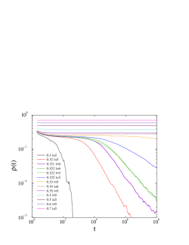
In order to determine the steady state behavior we first performed long runs, up to $T=10^{8}$ MCs, by starting the system from fully active state or from randomly half filled activity: $\rho(0)=0.5$. Fig. 9 shows the results for the excitatory model. At $\lambda=0.3$ the activity density falls exponentially fast to zero. We can see non-universal PL tails for $0.32\leq\lambda<0.33$, in agreement with the seed simulations. At $\lambda=0.33$ the density does not saturate to a constant value. Examining it on log.-lin. scale and performing average over thousands of independent samples it turns out that even the $\lambda=0.34$ curve decays very slowly. Only for $\lambda\geq 0.35$ we can see saturation, corresponding to active steady state, thus, we estimate $\lambda_{c}=0.345(5)$. We plotted the steady state saturation values on Fig. 10.

Figure 9: Evolution of $\rho(t)$ for different $\lambda$-s in case of starting from fully active state in the excitatory model with levels: $l=5,6$. From bottom to top symbols: $\lambda=$ 0.30, 0.32, 0.321 ($l=6$), 0.322, 0.322 ($l=6$), 0.325, 0.33, 0.34 (l=6), 0.35, 0.4, 0.5, 0.6, 0.7.

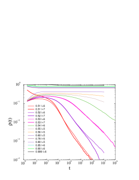
The same analysis has been done for the inhibitory and refractory-inhibitory cases and one can observe the shift of $\lambda_{c}$ to higher values as the consequence of the model modifications. We show the results for the inhibitory network on Fig. 11. Again, slow activity decays were observed, ending up with visible PL tails for $0.51\leq\lambda\leq 0.54$, while saturation starts from $\lambda_{c}\geq 0.80(1)$. The saturation value is $\rho_{c}=0.685(1)$, so the discontinuity is large. In the region $0.54<\lambda<0.80$ the curves do not saturate up to $T=10^{8}$ MCs, neither reach a scaling region. They belong to the inactive phase, but it is very difficult to distinguish them from other (logarithmic) decay forms.

Figure 10: Steady state behavior for the excitatory, inhibitory and refractory-inhibitory cases. Inset: evolution of $\rho$ in an inhibitory HMN2d with $N=4096$ for different initial activity densities: $\rho(0)=$ 0.0005, 0.001, 0.01, 0.1, 1 (bottom to top curves).

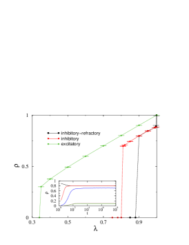
We can see large jumps at the transition points in all cases, suggesting a discontinuous transition above the GP. It is very hard to locate the exact location of the transition points as stability disappears very slowly. This suggests that at the critical point logarithmic decay occurs like in case of the disordered DP Vojta (2006).

Figure 11: Evolution of $\rho(t)$ for different $\lambda$-s, shown by legends in case of starting from active states in the inhibitory model. Thick, normal, thin lines correspond to $l=7$, $l=6$, $l=5$, accordingly. From bottom to top curves: $\lambda=$ 0.51, 0.52, 0.53, 0.54, 0.55, 0.56, 0.6, 0.78, 0.8, 0.85, 0.9, 0.999. The graph shows results with initial condition $\rho(0)=0.5$ for $\lambda\leq 0.6$, except for $\lambda=0.51$, $l=7$. In all the other cases $\rho(0)=1$ is applied.

We have also tried to start from other initial conditions than the full and single seed ones. As the inset of Fig. 10 shows we can see different saturation values for $\rho(0)<0.1$, that means we have multi-stability in case of low initial densities. This is the consequence of the fact that for low $\rho(0)$-s only parts of the graph can be activated. Even though the networks are simple connected and the lowest in-degree is $k_{i}^{in}=5$, not all nodes have $2$ incoming links from the same neighbor, which is necessary for the activation. These nodes cannot be activated by a neighbor if they are on the ”border” of an active territory, thus the graphs are practically fragmented from the activity point of view. This provides a mechanism for the emergence of GP even in high dimensions, without breaking conjecture provided in Muñoz et al. (2010), according to which GPs and similar RR effects do not exist in networks with an infinite topological dimension.

Furthermore, we can see the emergence of discontinuous transition with multi-stable states, which can be considered bi-stable, for initial excitation with node fraction $\rho(0)>0.1$ converging to an ”up” activity value, or by activation of single nodes, converging to a ”down” value.

VI Conclusions

In conclusion we provided numerical evidence that strong heterogeneity effects in networks, coming from the modular structure can result in GP even if the topological dimension is high, where mean-field scaling would be expected. This is the consequence of fragmented activity propagation caused by the modular topology and the threshold. We can define effective dimensions of the these graphs by running seed simulations with $\lambda=1$, $\nu=0$ and measuring $\rho(t)\sim t^{d_{eff}}$. For this compact growth $\rho(t)\sim N(r)$, so $d_{eff}$ provides an estimate for the dimensionality, similarly to the BFS algorithm. This is reminiscent of similar methods, for instance computing the spectral dimension of a network from random walk simulations  Burioni and Cassi (1996); Burioni et al. (2000); Burioni and Cassi (2005); Millán et al. (2019). While the topological dimension is a purely structural measure, $d_{eff}$, as well as the spectral dimension are observables of processes operating on networks, providing insights to dynamical signatures of localization, slowing down and dynamical fragmentation. However, it has recently been shown that in models of HMN-s the spectral dimension is not defined Esfandiary et al. (2020), thus our $d_{eff}$ can be a candidate to clarify relation of structure and slow dynamics. The inset of Fig. 8 shows that an initial scaling can be fitted for the excitatory case with: $\rho(t)\sim t^{1.84(3)}$, while for inhibitory: $\rho(t)\sim t^{1.19(1)}$. Thus these effective, activity dimensions are less than $d_{c}$, much smaller than the topological dimension obtained by the BFS, which is also shown on the graph as the function of $r$.

Furthermore, the threshold type models allow for the possibility to observe hybrid phase transitions, where order parameter discontinuity and multi-stability can co-exist with dynamical scaling in a GP, thus they can model brain criticality as well as up/down states. External activation can then push the model among the multi-stable states if it is poised near the transition point.

The investigated $K=2$ discrete threshold model results can obviously be extended for higher $K$ values and we expect to find similar behavior in continuous, integrate and fire type models on modular networks. Conversely, by duplicating the links we get back effectively the contact process Harris (1974) without RR effects and GP. For neural systems our results imply that the functional and structural connectivity can be different. The effects of inhibition and refractive states have also been studied and emergence of oscillatory states have been shown. Our model results are applicable to a wide range of phenomena, like power-grids, crack and fracture dynamics and contagion.

References

- Marro and Dickman (2005) J. Marro and R. Dickman, Nonequilibrium Phase Transitions in Lattice Models, Aléa-Saclay (Cambridge University Press, 2005), ISBN 9780521019460.
- Henkel et al. (2008) M. Henkel, H. Hinrichsen, and S. Lübeck, Non-equilibrium phase transition: Absorbing Phase Transitions (Springer Verlag, Netherlands, 2008).
- Ódor (2004) G. Ódor, Reviews of Modern Physics 76, 663 (2004).
- Ódor (2008) G. Ódor, Universality in nonequilibrium lattice systems: Theoretical foundations (World Scientific, 2008).
- Cardy (1981) J. L. Cardy, Journal of Physics A: Mathematical and General 14, 1407 (1981).
- Janssen et al. (2004) H.-K. Janssen, M. Müller, and O. Stenull, Physical Review E 70, 026114 (2004).
- Chan et al. (2015) W. Chan, F. Ghanbarnejad, and P. Grassberger, Nature Physics 11, 936– (2015).
- Dorogovtsev et al. (2006) S. N. Dorogovtsev, A. V. Goltsev, and J. F. F. Mendes, Physical Review Letters 96, 040601 (2006).
- Lee et al. (2016) D. Lee, S. Choi, M. Stippinger, J. Kertész, and B. Kahng, Physical Review E 93, 042109 (2016).
- Baxter et al. (2014) G. J. Baxter, S. N. Dorogovtsev, J. F. F. Mendes, and D. Cellai, Physical Review E 89, 042801 (2014).
- Bar and Mukamel (2014) A. Bar and D. Mukamel, Physical Review Letters 112, 015701 (2014).
- Juhász and Iglói (2017) R. Juhász and F. Iglói, Physical Review E 95, 022109 (2017).
- Grassberger (2017) P. Grassberger, Physical Review E 95, 010102(R) (2017).
- Juhász and Iglói (2018) R. Juhász and F. Iglói, Physical Review E 97, 012111 (2018).
- Pazó (2005) D. Pazó, Physical Review E 72, 046211 (2005).
- Gómez-Gardeñes et al. (2011) J. Gómez-Gardeñes, S. Gómez, A. Arenas, and Y. Moreno, Physical Review Letters 106, 128701 (2011).
- Coutinho et al. (2013) B. C. Coutinho, A. V. Goltsev, S. N. Dorogovtsev, and J. F. F. Mendes, Physical Review E 87, 032106 (2013).
- Haimovici et al. (2013) A. Haimovici, E. Tagliazucchi, P. Balenzuela, and D. R. Chialvo, Physical Review Letters 110, 178101 (2013).
- Johnson S. and Marro (2013) J. J. Johnson S., Torres and J. Marro, PLoS ONE 8, e50276 (2013).
- Bak et al. (1987) P. Bak, C. Tang, and K. Wiesenfeld, Physical Review Letters 59, 381 (1987).
- Chialvo (2010) D. R. Chialvo, Nature Physics 6, 744 (2010).
- Vojta (2006) T. Vojta, Journal of Physics A: Mathematical and General 39, R143 (2006).
- Griffiths (1969) R. B. Griffiths, Physical Review Letters 23, 17 (1969), ISSN 0031-9007.
- Ódor (2014) G. Ódor, Physical Review E 89, 042102 (2014).
- Karsai et al. (2018) M. Karsai, H.-H. Jo, and K. Kaski, SpringerBriefs in Complexity (2018), ISSN 2191-5334.
- Cota et al. (2016) W. Cota, S. C. Ferreira, and G. Ódor, Physical Review E 93, 032322 (2016).
- Imry and Ma (1975) Y. Imry and S.-k. Ma, Physical Review Letters 35, 1399 (1975).
- Aizenman and Wehr (1989) M. Aizenman and J. Wehr, Physical Review Letters 62, 2503 (1989).
- Villa Martín et al. (2014) P. Villa Martín, J. A. Bonachela, and M. A. Muñoz, Physical Review E 89, 012145 (2014).
- Villa Martín et al. (2015) P. Villa Martín, M. Moretti, and M. A. Muñoz, Journal of Statistical Mechanics p. P01003 (2015).
- Beggs and Plenz (2003) J. Beggs and D. Plenz, Journal Neuroscience 23, 11167 (2003).
- Tetzlaff et al. (2010) C. Tetzlaff, S. Okujeni, U. Egert, F. Wörgötter, and M. Butz, PLoS Computational Biology 6, e1001013 (2010).
- Hahn et al. (2010) G. Hahn, T. Petermann, M. N. Havenith, S. Yu, W. Singer, D. Plenz, and D. Nikolić, Journal of Neurophysiology 104, 3312 (2010), pMID: 20631221.
- Ribeiro et al. (2010) T. Ribeiro, M. Copelli, F. Caixeta, H. Belchior, D. Chialvo, M. Nicolelis, and S. Riberio, PLoS ONE 5, e14129 (2010).
- Ponce-Alvarez et al. (2018) A. Ponce-Alvarez, A. Jouary, M. Privat, G. Deco, and G. Sumbre, Neuron 100, 1446 (2018), ISSN 0896-6273.
- Muñoz (2018) M. A. Muñoz, Reviews of Modern Physics 90, 031001 (2018).
- Durstewitz et al. (2000) D. Durstewitz, J. K. Seamans, and T. J. Sejnowski, Nature Neuroscience 3, 1184 (2000).
- Kaltenbrunner et al. (2007) A. Kaltenbrunner, V. Gómez, and V. López, Neural Computation 19, 3011 (2007).
- Scarpetta et al. (2018) S. Scarpetta, I. Apicella, L. Minati, and A. de Candia, Physical Review E 97, 062305 (2018).
- Buendía et al. (2020) V. Buendía, P. Villegas, R. Burioni, and M. A. Muñoz, Hybrid-type synchronization transitions: where marginal coherence, scale-free avalanches, and bistability live together (2020), eprint arXiv:2011.03263.
- Kinouchi and Copelli (2006) O. Kinouchi and M. Copelli, Nature Physics 2, 348 (2006).
- Dobson et al. (2007) I. Dobson, B. A. Carreras, V. E. Lynch, and D. E. Newman, Chaos: An Interdisciplinary Journal of Nonlinear Science 17, 026103 (2007).
- Schäffer et al. (2018) B. Schäffer, D. Witthaut, M. Timme, and V. Latora, Nature Communications 9, 1975 (2018).
- Ódor and Hartmann (2018) G. Ódor and B. Hartmann, Physical Review E 98, 022305 (2018).
- Alava et al. (2006) M. J. Alava, P. K. V. V. Nukala, and S. Zapperi, Advances in Physics 55, 349–476 (2006), ISSN 1460-6976.
- Unicomb et al. (2018) S. Unicomb, G. Iniguez, and M. Karsai, Scientic Reports 8, 3094 (2018).
- Muñoz et al. (2010) M. A. Muñoz, R. Juhász, C. Castellano, and G. Ódor, Physical Review Letters 105, 128701 (2010).
- Ódor et al. (2015) G. Ódor, R. Dickman, and G. Ódor, Scientific Reports 5, 14451 (2015).
- Cota et al. (2018) W. Cota, G. Ódor, and S. C. Ferreira, Scientific Reports 8, 9144 (2018), ISSN 2045-2322.
- Gastner and Ódor (2016) M. Gastner and G. Ódor, Scientific Reports 6, 27249 (2016).
- Di Santo et al. (2018) S. Di Santo, P. Villegas, R. Burioni, and M. Muñoz, Proceedings of the National Academy of Sciences of the United States of America 115, E1356 (2018).
- Ódor (2003) G. Ódor, Physical Review E 67, 056114 (2003).
- Choi et al. (2018) W. Choi, D. Lee, J. Kertész, and B. Kahng, Physical Review E 98, 012311 (2018).
- Harris (1974) T. E. Harris, The Annals of Probability 2, 969 (1974).
- Kaiser and Hilgetag (2010) M. Kaiser and C. Hilgetag, Frontiers in Neuroinformatics 4 (2010).
- Latham and S. (2004) P. E. Latham and N. S., Neural Compuping 16, 1385 (2004).
- Barthelemy (2018) M. Barthelemy, Comptes Rendus Physique 19, 205–232 (2018), ISSN 1631-0705.
- Watts and Strogatz (1998) D. J. Watts and S. H. Strogatz, Nature 393, 440 (1998), ISSN 1476-4687.
- Fronczak et al. (2004) A. Fronczak, P. Fronczak, and J. A. Hołyst, Physical Review E 70, 056110 (2004).
- Humphries and Gurney (2008) M. D. Humphries and K. Gurney, PLOS ONE 3, 1 (2008).
- Palva et al. (2013) J. Palva, A. Zhigalov, J. Hirvonen, O. Korhonen, K. Linkenkaer-Hansen, and S. Palva, Proceedings of the National Academy of Sciences of the United States of America 110, 3585 (2013).
- Fontenele et al. (2019) A. J. Fontenele, N. A. P. de Vasconcelos, T. Feliciano, L. A. A. Aguiar, C. Soares-Cunha, B. Coimbra, L. Dalla Porta, S. Ribeiro, A. J. a. Rodrigues, N. Sousa, et al., Physical Review Letters 122, 208101 (2019).
- Moretti and Muñoz (2013) P. Moretti and M. A. Muñoz, Nature Communications 4, 2521 (2013).
- Ódor (2016) G. Ódor, Physical Review E 94, 062411 (2016).
- Ódor (2019) G. Ódor, Physical Review E 99, 012113 (2019).
- Moosavi et al. (2017) S. Moosavi, A. Montakhab, and A. Valizadeh, Scientific Reports 7, 7107 (2017).
- Zarepour et al. (2019) M. Zarepour, J. I. Perotti, O. V. Billoni, D. R. Chialvo, and S. A. Cannas, Physical Review E 100, 052138 (2019).
- Muñoz et al. (1999) M. A. Muñoz, R. Dickman, A. Vespignani, and S. Zapperi, Physical Review E 59, 6175 (1999).
- Burioni and Cassi (1996) R. Burioni and D. Cassi, Physical Review Letter 76, 1091 (1996).
- Burioni et al. (2000) R. Burioni, D. Cassi, and A. Vezzani, The European Physical Journal B 15, 665–672 (2000), ISSN 1434-6028.
- Burioni and Cassi (2005) R. Burioni and D. Cassi, Journal of Physics A: Mathematical and General 38, R45 (2005).
- Millán et al. (2019) A. P. Millán, J. J. Torres, and G. Bianconi, Physical Review E 99, 022307 (2019).
- Esfandiary et al. (2020) S. Esfandiary, A. Safari, J. Renner, P. Moretti, and M. A. Muñoz, Physical Review Research 2, 043291 (2020).