CPHT-RR090.112020, November 2020

One-loop masses of Neumann–Dirichlet open strings
and boundary-changing vertex operators

Thibaut Coudarchet and Hervé Partouche

CPHT, CNRS, Ecole Polytechnique, IP Paris,
F-91128 Palaiseau, France
thibaut.coudarchet@polytechnique.edu
herve.partouche@polytechnique.edu

  

Abstract

We derive the masses acquired at one loop by massless scalars in the Neumann–Dirichlet sector of open strings, when supersymmetry is spontaneously broken. It is done by computing two-point functions of “boundary-changing vertex operators” inserted on the boundaries of the annulus and Möbius strip. This requires the evaluation of correlators of “excited boundary-changing fields,” which are analogous to excited twist fields for closed strings. We work in the type IIB orientifold theory compactified on $T^{2}\times T^{4}/\mathbb{Z}_{2}$, where ${\cal N}=2$ supersymmetry is broken to ${\cal N}=0$ by the SSmechanism implemented along $T^{2}$. Even though the full expression of the squared masses is complicated, it reduces to a very simple form when the lowest scale of the background is the supersymmetry breaking scale $M_{3/2}$. We apply our results to analyze in this regime the stability at the quantum level of the moduli fields arising in the Neumann–Dirichlet sector. This completes the study of Ref. [32], where the quantum masses of all other types of moduli arising in the open- or closed-string sectors are derived. Ultimately, we identify all brane configurations that produce backgrounds without tachyons at one loop and yield an effective potential exponentially suppressed, or strictly positive with runaway behavior of $M_{3/2}$.

1 Introduction

Superstring-theory models based on two-dimensional conformal field theories of free fields have the advantage of allowing, at least in principle, string amplitudes to be computed exactly in string tension $\alpha^{\prime}$ by including all worldsheet instantons. Backgrounds whose internal spaces are $\mathbb{Z}_{N}$-twist orbifolds of tori are of particular interest since their numbers of spacetime supersymmetries are reduced in a “hard way” compared to the case of toroidal compactifications. In this framework, twisted states in the closed-string Hilbert space are mandatory for modular invariance to hold, which implies “twist fields” to exist in the conformal field theory to create them [1]. String amplitudes involving external states in the twisted sectors are based on correlation functions of twist fields, which are notoriously difficult to handle. Indeed, the seminal work of Ref. [2] presents results only for the case of twist fields creating ground states in the closed-string sector.

In open-string theory, the consistency of orbifold models also implies the presence of distinct D-brane sectors. For instance, in the type IIB orientifold on $T^{4}/\mathbb{Z}_{2}$ [3, 4, 5], open strings have either Neumann (N) or Dirichlet (D) boundary conditions in the orbifold directions, and are thus attached to D9- or D5-branes. In particular, strings with Neumann boundary conditions at one end and Dirichlet conditions at the other end populate the ND sector. In string amplitudes involving external states of this type, a conformal transformation maps the legs of the diagram to vertex operators localized along the worldsheet boundary. The key point is that the nature of an ND-sector state implies that the worldsheet boundary condition changes from Neumann on one side of the vertex to Dirichlet on the other side. Hence, vertex operators creating states in the ND sector involve “boundary-changing fields” [6] dressed by other objects encoding the quantum numbers.

It turns out that twist fields and boundary-changing fields have identical OPE’s [6, 2], up to the fact that the former are inserted in the bulk of the worldsheet and the latter on the boundary. Combining this with the method of images which defines surfaces with boundaries as Rienmann surfaces modded by involutions [7, 8], correlation functions of boundary-changing fields can be related to those of twist fields. In the literature, this point of view was applied for computing amplitudes with external states of ND sectors in supersymmetric theories at tree level [9, 10, 11, 12] and one loop [13, 14, 15, 16, 17, 18], while other approaches were followed in Refs. [19, 20, 21].

In the present work, we consider the type IIB orientifold model of Refs. [3, 4, 5] compactified on $T^{2}\times T^{4}/\mathbb{Z}_{2}$, when ${\cal N}=2$ supersymmetry is spontaneously broken to ${\cal N}=0$. The implementation of the breaking consists of a string version [22, 23, 24, 25, 26, 27, 28, 29] of the SSmechanism [30, 31] along one direction of $T^{2}$. In this case, the supersymmetry breaking scale, $M_{3/2}$, is a modulus inversely proportional to the size of the compact direction involved in the mechanism. Moreover, the free nature of the bosonic and fermionic fields defining the worldsheet conformal field theory is preserved and the results of Ref. [2] apply. An effective potential which depends on all moduli fields is generated by quantum corrections and the question of their stability must be addressed. Assuming the string coupling to be in perturbative regime, loci in moduli space where the one-loop effective potential is extremal with respect to all moduli fields except $M_{3/2}$ have been determined in Ref. [32], up to exponentially suppressed terms. At these points, the potential reads

$${\cal V}_{\mbox{\scriptsize 1-loop}}=\upsilon(n_{\rm F}-n_{\rm B})M_{3/2}^{4}+{\cal O}\!\left((M_{\rm s}M_{3/2})^{2}\,e^{-\pi\frac{cM_{\rm s}}{M_{3/2}}}\right),$$ (1.1)

where $n_{\rm F}$ and $n_{\rm B}$ are the numbers of massless fermionic and bosonic degrees of freedom present at genus-0. Moreover, $\upsilon>0$ is a constant, $M_{\rm s}\equiv 1/\sqrt{\alpha^{\prime}}$ is the string scale, and $cM_{\rm s}$ is the lowest non-vanishing mass scale other than $M_{3/2}$, $0<c\leq 1$. Hence, Eq. (1.1) is of interest in all regions in moduli space where $cM_{\rm s}$, which is a compactification scale, is greater than $M_{3/2}$. When this is the case and the exponential contributions are neglected, $M_{3/2}$ runs away, except when the background satisfies a Bose/Fermi degeneracy at genus-0, $n_{\rm F}-n_{\rm B}=0$, implying $M_{3/2}$ to be a flat direction (for other theories, see Refs. [33, 34, 35, 36, 37, 38, 39, 40, 41, 42, 43]). For arbitrary $n_{\rm F}-n_{\rm B}$, though, stability of all remaining moduli fields can be analyzed from different points of view.

In Ref. [32], the mass terms of all moduli fields in the NN and DD open-string sectors were derived by direct computation of the potential for arbitrary backgrounds of these scalars. The untwisted closed-string sector contains three types of moduli fields: Firstly, since the internal metric components do not show up in the dominant term of Eq. (1.1) (except the combination $M_{3/2}$), they parametrize flat directions up to the suppressed terms. Secondly, heterotic/type I duality was used to show that the Ramond-Ramond (RR) two-form moduli are also flat directions. Finally, the same conclusion definitely applies to the dilaton at one loop. The twisted closed-string sector contains 16 blowing-up modes of $T^{4}/\mathbb{Z}_{2}$ among which 2 to 16 are absorbed by anomalous $U(1)$’s, which become massive vector fields thanks to a generalized Green–Schwarz mechanism. In this regard, the present work can be seen as a companion paper of Ref. [32], as it provides a derivation of the mass terms generated at one loop by the remaining moduli fields, namely those belonging to the ND+DN open-string sector. This will be done by computing two-point functions of boundary-changing vertex operators of massless scalars in the ND+DN sector, on the annulus and Möbius strip.

In Sect. 2, we review the description of the type IIB orientifold model with broken ${\cal N}=2$ supersymmetry, which involves D9- and D5-branes. Alternative T-dual pictures are also introduced for describing the NN- and DD-sector moduli as positions of D3-branes in the internal space. Sect. 3 defines the string amplitudes we are interested in. Sect. 4 presents all correlators needed to calculate these amplitudes on the double-cover tori of the annulus and Möbius strip. In particular, we review the derivation of Ref. [2] of the correlation function of twist fields that create ground states in the twisted sectors of closed strings. Following the method introduced in Refs. [13, 14, 15, 16, 17], we extend the result to the case of “excited twist fields” i.e. operators appearing as higher order terms in the OPE of ordinary twist fields.

In Sect. 5 we compute the two-point functions of interest. While the formulas can be used to extract the one-loop corrections to the Kähler metric and masses of the classically massless scalars of the ND+DN sector, they turn out to be rather cumbersome and obscure. For this reason, we derive in Sect. 6 a simplified expression of the squared masses at one loop that is valid when $M_{3/2}$ is lower than all other non-vanishing mass scales present in the background, precisely in the spirit of Eq. (1.1) which holds in this regime.

In Sect. 7, we apply this result to the last two models highlighted in Ref. [32], which presented all brane configurations that are tachyon free (or potentially tachyon free) at one loop and satisfy $n_{\rm F}-n_{\rm B}\geq 0$. The outcome of the two papers is that among the ${\cal O}(10^{11})$ non-perturbatively consistent brane configurations, there exist 2 tachyon free setups with $n_{\rm F}-n_{\rm B}=0$, and 5 with $n_{\rm F}-n_{\rm B}>0$. A third configuration with $n_{\rm F}-n_{\rm B}=0$ and ND+DN-sector moduli is tachyon free at one loop, up to 2 blowing-up modes of $T^{4}/\mathbb{Z}_{2}$ for which we have not computed the quantum mass terms.

Finally, our conclusions can be found in Sect. 8, while technical points are reported in three appendices.

2 The ${\cal N}=2\to{\cal N}=0$ open-string model

In this section, we review the open-string model considered in Ref. [32, 44], which realizes at tree level the spontaneous breaking of ${\cal N}=2$ supersymmetry in four-dimensional Minkowski spacetime. Our goals are to fix our notations, list the massless spectrum at genus-0, and specify the moduli fields whose masses will be computed at one loop in the sections to come.

2.1 The supersymmetric parent model

At the supersymmetric level, our starting point is the type IIB orientifold model constructed in six dimensions by Bianchi and Sagnotti [3], as well as by Gimon and Polchinski [4, 5]. Compactified down to four dimensions, the full gravitational background becomes

$$\mathbb{R}^{1,3}\times T^{2}\times{T^{4}\over\mathbb{Z}_{2}}\,,$$ (2.2)

whose coordinates will be labeled by Greek, primed Latin and unprimed Latin indices

spacetime: $$X^{\mu}\,, \leavevmode\nobreak\ \leavevmode\nobreak\ \mu\in\{0,\dots,3\}\,,$$ (2.3)

two-torus: $$X^{I^{\prime}}\,, \leavevmode\nobreak\ \leavevmode\nobreak\ I^{\prime}\in\{4,5\}\,,$$

four-torus: $$X^{I}\,, \leavevmode\nobreak\ \leavevmode\nobreak\ I\in\{6,\dots,9\}\,,$$

and where the $\mathbb{Z}_{2}$-orbifold generator is defined as

$$g:\quad(X^{6},X^{7},X^{8},X^{9})\longrightarrow(-X^{6},-X^{7},-X^{8},-X^{9})\,.$$ (2.4)

The background also contains orientifold planes and D-branes. First of all, there is an O9-plane and 32 D9-branes spanned along all spatial directions. Second, there is an O5-plane localized at each of the 16 fixed points of $T^{4}/\mathbb{Z}_{2}$, and 32 D5-branes transverse to $T^{4}/\mathbb{Z}_{2}$. Open strings with one end attached to a D9-brane have Neumann boundary conditions in all spacetime coordinates, while those stuck to a D5-brane have Dirichlet boundary conditions along the directions of $T^{4}/\mathbb{Z}_{2}$ (and Neumann along $\mathbb{R}^{1,3}\times T^{2}$).

Moduli fields:

• On the worldvolumes of the 32 D5-branes, the gauge bosons can develop vacuum expectation values (vev’s) along $T^{2}$, which are Wilson lines. T-dualizing the two-torus, the 32 D5-branes become D3-branes whose positions along $\tilde{X}^{I^{\prime}}$, the coordinates along the T-dual torus $\tilde{T}^{2}$ of metric $\tilde{G}_{I^{\prime}J^{\prime}}\equiv G^{I^{\prime}J^{\prime}}$, are nothing but the Wilson-line moduli of the original description [45]. Because in the T-dual picture a D3-brane at $(\tilde{X}^{I^{\prime}},X^{I})$ is transformed under $\Omega$, the orientifold generator, into an “orientifold-mirror” D3-brane located at $(-\tilde{X}^{I^{\prime}},-X^{I})$ [45], there are 64 fixed points in this description, all supporting one O3-plane. Moreover, at genus-0, there are only 16 independent positions along $\tilde{T}^{2}$, which are associated with the brane/mirror brane pairs.

• The locations of the 32 D3-branes (T-dual to the D5-branes) in $T^{4}/\mathbb{Z}_{2}$ are also allowed to vary, provided this is done consistently with the symmetries generated by $g$ and $\Omega$. Indeed, a D3-brane sitting at $(\tilde{X}^{I^{\prime}},X^{I})$ must be paired with an image brane under $g$ at $(\tilde{X}^{I^{\prime}},-X^{I})$. Moreover, both admit “mirror branes” under $\Omega$, which are located at $(-\tilde{X}^{I^{\prime}},-X^{I})$ and $(-\tilde{X}^{I^{\prime}},X^{I})$. Hence, there are at most 8 independent D3-brane positions in $T^{4}/\mathbb{Z}_{2}$. Notice that this number is lowered when there are $2$ modulo 4 D3-branes sitting on one of the 64 O3-planes, since such a configuration is still symmetric under $g$ and $\Omega$ but does not allow 2 D3-branes to move in the bulk of $T^{4}/\mathbb{Z}_{2}$. In other words, 2 D3-branes have rigid positions in $T^{4}/\mathbb{Z}_{2}$.

• Applying a T-duality on the four-torus of the background (2.2), D5-branes and D9-branes are turned into each other. Therefore, all moduli fields described for the D5-branes admit counterparts for the D9-branes. In particular, the D9-brane moduli are mapped into positions of 32 D3-branes in $\tilde{T}^{2}\times\tilde{T}^{4}/\mathbb{Z}_{2}$, where $\tilde{T}^{4}$ is the dual four-torus with metric $\tilde{G}_{IJ}\equiv G^{IJ}$ and coordinates $\tilde{X}^{I}$. In this alternative T-dual picture, there are again 64 O3-planes at the fixed points of the inversion $(\tilde{X}^{I^{\prime}},\tilde{X}^{I})\to(-\tilde{X}^{I^{\prime}},-\tilde{X}^{I})$.

• In the original picture involving D5- and D9-branes, all open-string moduli described so far correspond to modes realized in the DD and NN sectors. However, open strings stretched between one D5-brane and one D9-brane can also lead to moduli fields. The present paper is devoted to the study of these moduli. To be specific, we will derive the masses they acquire at one loop, when supersymmetry is spontaneously broken and their vev’s vanish. When these moduli condense, the backgrounds can be described in terms of brane recombinations or magnetized branes [46, 47, 48, 49].

Geometric picture:

In order to specify a particular set of vev’s for the moduli arising from the DD and NN sectors, we will use a pictorial representation [32], as shown in Fig. 1(a).

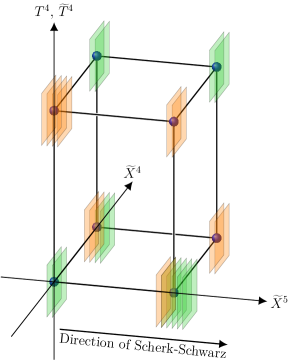
(a) Configuration of D3-branes associated with D5-branes (orange) and D9-branes (green) in T-dual pictures. In this example, all D3-branes sit on O3-planes (blue dots).

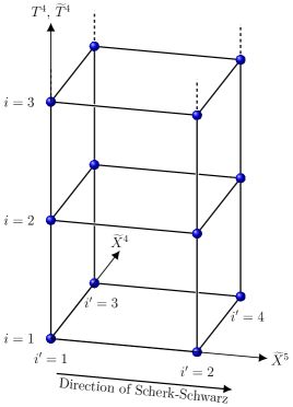
(b) Labelling of the fixed points $i^{\prime}\in\{1,...,4\}$ along the directions of $\tilde{T}^{2}$, and schematic labelling of the fixed points $i\in\{1,...,16\}$ along the directions of $T^{4}$ or $\tilde{T}^{4}$. $i^{\prime}=1$ or 3 correspond to points at $\tilde{X}^{5}=0$, while $i^{\prime}=2$ or 4 correspond to points at $\tilde{X}^{5}=\pi$, where $\tilde{X}^{5}$ is the coordinate T-dual to the direction along which the Scherk–Schwarz mechanism is implemented.

Figure 1: Description in terms of D3-brane positions of the moduli arising from the NN and DD sectors of the orientifold theory.

We represent the fundamental domain of $\tilde{T}^{2}\times T^{4}/\mathbb{Z}_{2}$ modded by the involution $(\tilde{X}^{I^{\prime}},X^{I})\to(-\tilde{X}^{I^{\prime}},-X^{I})$ by a schematic six-dimensional “box”, with an O3-plane represented by a dot at each fixed point i.e. corner of the box. The moduli in the DD sector correspond to the positions of the 32 D3-branes (drawn in orange) T-dual to the D5-branes. Similarly, we consider a second box corresponding to the fundamental domain of $\tilde{T}^{2}\times\tilde{T}^{4}/\mathbb{Z}_{2}$ modded by the involution $(\tilde{X}^{I^{\prime}},\tilde{X}^{I})\to(-\tilde{X}^{I^{\prime}},-\tilde{X}^{I})$, with the moduli of the NN sector given by the positions of the 32 D3-branes (drawn in green) T-dual to the D9-branes. Finally, we superpose the two boxes, keeping in mind that the resulting picture combines information from two distinct T-dual descriptions of the same theory.

In the schematic example of Fig. 1(a), all D3-branes are located on O3-planes. Indeed, it has been shown in Ref. [32] that in presence of supersymmetry breaking (to be introduced in the next subsection) these configurations are of particular interest, since they yield extrema of the one-loop effective potential with respect to the moduli arising from the NN and DD sectors (except for $M_{3/2}$ when $n_{\rm F}\neq n_{\rm B}$), up to exponentially suppressed terms (see Eq. (1.1)). Therefore, from now on, we will consider background values of the moduli in the DD and NN sectors corresponding to stacks of D3-branes all located on corners of the six-dimensional boxes. To this end, we label the 64 corners by a double index $ii^{\prime}$, where $i\in\{1,\dots,16\}$ refers to the fixed points of $T^{4}/\mathbb{Z}_{2}$ (or $\tilde{T}^{4}/\mathbb{Z}_{2}$), and $i^{\prime}\in\{1,\dots,4\}$ is associated with those in the $\tilde{T}^{2}$ directions. Hence, the coordinates of corner $ii^{\prime}$ are captured by a two-vector $2\pi\vec{a}_{i^{\prime}}$ and a four-vector $2\pi\vec{a}_{i}$, whose components satisfy

$$a_{i^{\prime}}^{I^{\prime}}\,,\leavevmode\nobreak\ a_{i}^{I}\in\left\{0,\frac{1}{2}\right\},\quad i^{\prime}\in\{1,\dots,4\}\,,\leavevmode\nobreak\ \leavevmode\nobreak\ i\in\{1,\dots,16\}\,.$$ (2.5)

Fig. 1(b) shows how the labelling looks like when the fixed points $i\in\{1,\dots,16\}$ are schematically arranged linearly along a vertical axis. In these notations, we will denote by $D_{ii^{\prime}}$ and $N_{ii^{\prime}}$ the numbers of D3-branes T-dual to the D5-branes and D9-branes that are located at corners $ii^{\prime}$ of the appropriate boxes.

2.2 Spontaneous supersymmetry breaking

In quantum field theory, the SSmechanism amounts to imposing fields to satisfy boundary conditions along compact directions that are compatible with global symmetries and depend on associated conserved charges [30, 31]. When charges vary between superpartners, distinct Kaluza–Klein masses arise in lower dimension and supersymmetry is spontaneously broken. The implementation of this mechanism in closed-string theory was developed in Refs. [50, 51, 52, 53, 54], and extended to the open-string framework in Refs. [22, 23, 24, 25, 26, 27, 28, 29].

In the model based on the background (2.2), we make the choice to implement the SSmechanism along the periodic direction $X^{5}$ only, and to use the fermionic number $F$ as conserved charge. In practice, $F=0$ for the bosonic degrees of freedom and $F=1$ for the fermionic ones. Denoting $\vec{m}^{\prime}$ the two-vector whose components are the Kaluza–Klein momenta $(m_{4},m_{5})\in\mathbb{Z}^{2}$ along $T^{2}$, the lattices of zero modes appearing in the one-loop partition function are shifted according to the rules

$$\vec{m}^{\prime}+F\,\vec{a}^{\prime}_{\rm S} \quad\mbox{for closed string}\,,$$ (2.6)

$$\vec{m}^{\prime}+F\,\vec{a}^{\prime}_{\rm S}+\vec{a}_{i^{\prime}}-\vec{a}_{j^{\prime}} \quad\mbox{for open string}\,,$$

where we have defined

$$\vec{a}^{\prime}_{\rm S}=\left(0,\frac{1}{2}\right).$$ (2.7)

As a result, the two gravitino masses are

$$M_{3/2}=\frac{\sqrt{G^{55}}}{2}\,M_{\rm s}\,,$$ (2.8)

which is the scale of ${\cal N}=2\to{\cal N}=0$ spontaneous breaking of supersymmetry. In the open-string case, the extra shift $\vec{a}_{i^{\prime}}-\vec{a}_{j^{\prime}}$ arises from the Wilson-line background along $T^{2}$ of the gauge fields living on the worldvolumes of the D5- and D9-branes. In the D3-brane T-dual pictures, it means that an open string is stretched between D3-branes sitting on corners $ii^{\prime}$ and $jj^{\prime}$, regardless of whether they are dual to D5- or D9-branes. Because of the particular role played by the direction $\tilde{X}^{5}$, which is T-dual to the SSdirection $X^{5}$ of the original picture, it is convenient to specify our labelling of the fixed points along the directions of $\tilde{T}^{2}$. We will denote by $i^{\prime}=1$ and 3 those located at $\tilde{X}^{5}=0$, and by $i^{\prime}=2$ and 4 those located at $\tilde{X}^{5}=\pi$ (see Fig. 1(b)).

Partition function:

The one-loop partition function can be divided into four contributions $Z_{\Sigma}$, which can be derived from path integrals on worldsheets whose topologies are those of a torus $({\cal T})$, Klein bottle $({\cal K})$, annulus $({\cal A})$ and Möbius strip $({\cal M})$. These contributions can also be expressed as supertraces over the modes belonging to the untwisted and twisted closed-string sectors, as well as over those in the NN, DD, ND and DN open-string sectors. For the closed strings, we have

$$Z_{\cal T}={1\over\tau_{2}^{2}}\,\textrm{Str}\,\frac{1}{2}\,\frac{1+g}{2}\,q^{L_{0}-\frac{1}{2}}\,\bar{q}^{\tilde{L}_{0}-\frac{1}{2}}\,,\quad Z_{\cal K}={1\over\tau_{2}^{2}}\,\textrm{Str}\,{\Omega\over 2}\,\frac{1+g}{2}\,q^{L_{0}-\frac{1}{2}}\,\bar{q}^{\tilde{L}_{0}-\frac{1}{2}}\,,\quad q=e^{2i\pi\tau}\,,$$ (2.9)

where $\tau$ is the Teichmüller parameter of the worldsheet torus with real and imaginary parts denoted $\tau_{1}$ and $\tau_{2}>0$, while for the open strings we have

$$Z_{\cal A}={1\over\tau_{2}^{2}}\,\textrm{Str}\,\frac{1}{2}\,\frac{1+g}{2}\,q^{\frac{1}{2}(L_{0}-1)}\,,\qquad Z_{\cal M}={1\over\tau_{2}^{2}}\,\textrm{Str}\,{\Omega\over 2}\,\frac{1+g}{2}\,q^{\frac{1}{2}(L_{0}-1)}\,,\qquad q=e^{-2\pi\tau_{2}}\,.$$ (2.10)

In these formulas, $L_{0}$, $\tilde{L}_{0}$ are the zero-frequency Virasoro operators.

In order to give explicit expressions of $Z_{\cal A}$ and $Z_{\cal M}$, we first define four-vectors $\vec{m}$ and $\vec{n}$ whose components are the Kaluza–Klein momenta $m_{I}\in\mathbb{Z}$ and winding numbers $n_{I}\in\mathbb{Z}$ along the directions of $T^{4}$. The lattices of zero modes (to be shifted by Wilson lines) of the bosonic coordinates are then given by

$$\sum_{\vec{m}}P_{\vec{m}}^{(4)}(i\tau_{2}) =\sum_{\vec{m}}e^{-\pi\tau_{2}m_{I}G^{IJ}m_{J}} \quad\mbox{for the NN sector}\,,$$ (2.11)

$$\sum_{\vec{n}}W_{\vec{n}}^{(4)}(i\tau_{2}) =\sum_{\vec{n}}e^{-\pi\tau_{2}n_{I}G_{IJ}n_{J}} \quad\mbox{for the DD sector}\,,$$

$$\leavevmode\nobreak\ \,1 \quad\mbox{for the ND and DN sectors}\,,$$

while the lattice of momenta along $T^{2}$ is

$$\sum_{\vec{m}^{\prime}}P_{\vec{m}^{\prime}}^{(2)}(i\tau_{2})=\sum_{\vec{m}^{\prime}}e^{-\pi\tau_{2}m_{I^{\prime}}G^{I^{\prime}J^{\prime}}m_{J^{\prime}}}$$ (2.12)

in all open-string sectors.

In the annulus contribution to the partition function, the actions of the neutral group element 1 and generator $g$ on the Chan–Paton indices can be represented by matrices acting on each Neumann or Dirichlet sector $ii^{\prime}$ [4, 5],

$$\gamma^{ii^{\prime}}_{{\rm N},1}=I_{N_{ii^{\prime}}}\,,\leavevmode\nobreak\ \leavevmode\nobreak\ \quad \gamma^{ii^{\prime}}_{{\rm N},g}=J_{N_{ii^{\prime}}}\,,$$ (2.13)

$$\gamma^{ii^{\prime}}_{{\rm D},1}=I_{D_{ii^{\prime}}}\,,\leavevmode\nobreak\ \leavevmode\nobreak\ \quad \gamma^{ii^{\prime}}_{{\rm D},g}=J_{D_{ii^{\prime}}}\,,$$

where $I_{k}$ is the $k\times k$ identity matrix while for $k$ even

$$J_{k}=\begin{pmatrix}0&I_{k\over 2}\\ -I_{k\over 2}&0\end{pmatrix}.$$ (2.14)

Actually, the precise dictionary between the above matrices and those defined in Refs. [4, 5] can be found in Appendix A. To be specific, by labelling the branes with Greek indices, the actions of $G=1$ or $g$ are represented in the NN sector as follows:

$$\forall\alpha\in\{1,\dots,N_{ii^{\prime}}\}\,,\forall\beta\in\{1,\dots,N_{jj^{\prime}}\}\,,\quad|\alpha\beta\rangle\to\sum_{\alpha^{\prime}=1}^{N_{ii^{\prime}}}\sum_{\beta^{\prime}=1}^{N_{jj^{\prime}}}(\gamma^{ii^{\prime}}_{{\rm N},G})_{\alpha\alpha^{\prime}}|\alpha^{\prime}\beta^{\prime}\rangle(\gamma^{jj^{\prime}\,-1}_{{\rm N},G})_{\beta^{\prime}\beta}\,.$$ (2.15)

Similar expressions apply to the DD sector for $G=1$, $g$, as well as to the ND and DN sectors for $G=1$. There exists only one subtlety in the ND and DN sectors for $G=g$, where one has to multiply all Neumann matrices by signs in the transformation rules,

$$\gamma_{{\rm N},g}^{ii^{\prime}}\leavevmode\nobreak\ \leavevmode\nobreak\ \longrightarrow\leavevmode\nobreak\ \leavevmode\nobreak\ e^{4i\pi\vec{a}_{i}\cdot\vec{a}_{j}}\gamma_{{\rm N},g}^{ii^{\prime}}\,,$$ (2.16)

where the index $j$ refers to the fixed point of $T^{4}/\mathbb{Z}_{2}$ where the stack of D5-branes sits. This is explained in Ref. [5] and translated into the notations of our paper in Appendix A. Moreover, the worldsheet fermions associated with the directions $X^{2},\dots,X^{5}$ on the one-hand, and those associated with the directions $X^{6},\dots,X^{9}$ on the other hand, yield contributions expressed as characters of the $SO(4)$ affine algebra. The latter are associated with a singlet (O), vectorial (V) and two spinorial (S and C) conjugacy classes [55, 56, 57]. For the annulus partition function, these characters denoted $O_{4}$, $V_{4}$, $S_{4}$, $C_{4}$ are defined in Eq. (B.206) and evaluated at argument $i\tau_{2}/2$. Altogether, one obtains

$$Z_{\cal A}={1\over 4}\,{1\over\tau_{2}^{2}}\sum_{\begin{subarray}{c}i,i^{\prime}\\ j,j^{\prime}\end{subarray}}$$

$$\bigg{\{}\bigg{[}(V_{4}O_{4}+O_{4}V_{4})\bigg{(}\textrm{tr}(\gamma_{{\rm N},1}^{ii^{\prime}})\textrm{tr}(\gamma_{{\rm N},1}^{jj^{\prime}\,-1})\sum_{\vec{m}}{P^{(4)}_{\vec{m}+\vec{a}_{i}-\vec{a}_{j}}\over\eta^{4}}+\textrm{tr}(\gamma_{{\rm D},1}^{ii^{\prime}})\textrm{tr}(\gamma_{{\rm D},1}^{jj^{\prime}\,-1})\sum_{\vec{n}}{W^{(4)}_{\vec{n}+\vec{a}_{i}-\vec{a}_{j}}\over\eta^{4}}\bigg{)}$$

$$-(V_{4}O_{4}-O_{4}V_{4})\,\delta_{ij}\,\big{(}\textrm{tr}(\gamma_{{\rm N},g}^{ii^{\prime}})\textrm{tr}(\gamma_{{\rm N},g}^{jj^{\prime}\,-1})+\textrm{tr}(\gamma_{{\rm D},g}^{ii^{\prime}})\textrm{tr}(\gamma_{{\rm D},g}^{jj^{\prime}\,-1})\big{)}\left(\frac{2\eta}{\vartheta_{2}}\right)^{2}$$

$$+(O_{4}C_{4}+V_{4}S_{4})\big{(}\textrm{tr}(\gamma_{{\rm N},1}^{ii^{\prime}})\textrm{tr}(\gamma_{{\rm D},1}^{jj^{\prime}\,-1})+\textrm{tr}(\gamma_{{\rm D},1}^{ii^{\prime}})\textrm{tr}(\gamma_{{\rm N},1}^{jj^{\prime}\,-1})\big{)}\left(\frac{\eta}{\vartheta_{4}}\right)^{2}\phantom{\!\!\overset{\displaystyle|}{|}}$$ (2.17)

$$-(O_{4}C_{4}-V_{4}S_{4})\,e^{4i\pi\vec{a}_{i}\cdot\vec{a}_{j}}\big{(}\textrm{tr}(\gamma_{{\rm N},g}^{ii^{\prime}})\textrm{tr}(\gamma_{{\rm D},g}^{jj^{\prime}\,-1})+\textrm{tr}(\gamma_{{\rm D},g}^{ii^{\prime}})\textrm{tr}(\gamma_{{\rm N},g}^{jj^{\prime}\,-1})\big{)}\left(\frac{\eta}{\vartheta_{3}}\right)^{2}\bigg{]}\sum_{\vec{m}^{\prime}}\frac{P^{(2)}_{\vec{m}^{\prime}+\vec{a}_{i^{\prime}}-\vec{a}_{j^{\prime}}}}{\eta^{4}}$$

$$-\bigg{[}(S_{4}S_{4}+C_{4}C_{4})\bigg{(}\textrm{tr}(\gamma_{{\rm N},1}^{ii^{\prime}})\textrm{tr}(\gamma_{{\rm N},1}^{jj^{\prime}\,-1})\sum_{\vec{m}}{P^{(4)}_{\vec{m}+\vec{a}_{i}-\vec{a}_{j}}\over\eta^{4}}+\textrm{tr}(\gamma_{{\rm D},1}^{ii^{\prime}})\textrm{tr}(\gamma_{{\rm D},1}^{jj^{\prime}\,-1})\sum_{\vec{n}}{W^{(4)}_{\vec{n}+\vec{a}_{i}-\vec{a}_{j}}\over\eta^{4}}\bigg{)}$$

$$-(C_{4}C_{4}-S_{4}S_{4})\,\delta_{ij}\,\big{(}\textrm{tr}(\gamma_{{\rm N},g}^{ii^{\prime}})\textrm{tr}(\gamma_{{\rm N},g}^{jj^{\prime}\,-1})+\textrm{tr}(\gamma_{{\rm D},g}^{ii^{\prime}})\textrm{tr}(\gamma_{{\rm D},g}^{jj^{\prime}\,-1})\big{)}\left(\frac{2\eta}{\vartheta_{2}}\right)^{2}$$

$$+(S_{4}O_{4}+C_{4}V_{4})\big{(}\textrm{tr}(\gamma_{{\rm N},1}^{ii^{\prime}})\textrm{tr}(\gamma_{{\rm D},1}^{jj^{\prime}\,-1})+\textrm{tr}(\gamma_{{\rm D},1}^{ii^{\prime}})\textrm{tr}(\gamma_{{\rm N},1}^{jj^{\prime}\,-1})\big{)}\left(\frac{\eta}{\vartheta_{4}}\right)^{2}\phantom{\!\!\overset{\displaystyle|}{|}}$$

$$-(S_{4}O_{4}-C_{4}V_{4})\,e^{4i\pi\vec{a}_{i}\cdot\vec{a}_{j}}\big{(}\textrm{tr}(\gamma_{{\rm N},g}^{ii^{\prime}})\textrm{tr}(\gamma_{{\rm D},g}^{jj^{\prime}\,-1})+\textrm{tr}(\gamma_{{\rm D},g}^{ii^{\prime}})\textrm{tr}(\gamma_{{\rm N},g}^{jj^{\prime}\,-1})\big{)}\left(\frac{\eta}{\vartheta_{3}}\right)^{2}\bigg{]}\sum_{\vec{m}^{\prime}}\frac{P^{(2)}_{\vec{m}^{\prime}+\vec{a}^{\prime}_{\text{S}}+\vec{a}_{i^{\prime}}-\vec{a}_{j^{\prime}}}}{\eta^{4}}\bigg{\}}\,.$$

In the the Möbius-strip contribution to the partition function, the actions of $\Omega$ and $\Omega g$ on the Chan–Paton indices can be represented by matrices associated with each Neumann or Dirichlet sector $ii^{\prime}$,

$$\gamma^{ii^{\prime}}_{{\rm N},\Omega}\leavevmode\nobreak\ =I_{N_{ii^{\prime}}}\,,\leavevmode\nobreak\ \leavevmode\nobreak\ \quad \gamma^{ii^{\prime}}_{{\rm N},\Omega g}=J_{N_{ii^{\prime}}}\,,$$ (2.18)

$$\gamma^{ii^{\prime}}_{{\rm D},\Omega g}=I_{D_{ii^{\prime}}}\,,\leavevmode\nobreak\ \leavevmode\nobreak\ \quad \gamma^{ii^{\prime}}_{{\rm D},\Omega}\leavevmode\nobreak\ =J_{D_{ii^{\prime}}}\,.$$

Notice the inverted roles of $\Omega$ and $\Omega g$ in the Neumann and Dirichlet sectors. The precise actions of $\Omega G$ for $G=1$ or $g$ on the NN sector are [4]

$$\forall\alpha\in\{1,\dots,N_{ii^{\prime}}\}\,,\forall\beta\in\{1,\dots,N_{jj^{\prime}}\}\,,\leavevmode\nobreak\ \leavevmode\nobreak\ \leavevmode\nobreak\ |\alpha\beta\rangle\to\sum_{\alpha^{\prime}=1}^{N_{ii^{\prime}}}\sum_{\beta^{\prime}=1}^{N_{jj^{\prime}}}(\gamma^{ii^{\prime}}_{{\rm N},\Omega G})_{\alpha\alpha^{\prime}}|\beta^{\prime}\alpha^{\prime}\rangle(\gamma^{jj^{\prime}\,-1}_{{\rm N},\Omega G})_{\beta^{\prime}\beta}\,,$$ (2.19)

and similarly for the DD sector. As compared to Eq. (2.15), note the reversal $\alpha^{\prime}\beta^{\prime}\to\beta^{\prime}\alpha^{\prime}$ in the transformation rule. As a result, the ND and DN sectors automatically yield vanishing contributions in the defining trace of $Z_{\cal M}$. Moreover, all characters denoted generically as $\hat{\chi}$ appearing in the Möbius strip partition function can be defined in terms of their counterparts $\chi$ in the annulus amplitude by the relation [58, 59]

$$\hat{\chi}\Big{(}\frac{1}{2}+i{\tau_{2}\over 2}\Big{)}=e^{-i\pi(h-{c\over 24})}\,\chi\Big{(}\frac{1}{2}+i{\tau_{2}\over 2}\Big{)}\,,$$ (2.20)

where $h$ is the weight of the associated primary state and $c$ the central charge of the Verma module. With these notations, one obtains

$$Z_{\cal M}= -{1\over 4}\,\sum_{i,i^{\prime}}\bigg{\{}\bigg{[}(\hat{V}_{4}\hat{O}_{4}+\hat{O}_{4}\hat{V}_{4})\bigg{(}\textrm{tr}(\gamma_{{\rm N},\Omega}^{ii^{\prime}\,{\rm T}}\gamma_{{\rm N},\Omega}^{ii^{\prime}\,-1})\sum_{\vec{m}}{P^{(4)}_{\vec{m}}\over\hat{\eta}^{4}}+\textrm{tr}(\gamma_{{\rm D},\Omega g}^{ii^{\prime}\,{\rm T}}\gamma_{{\rm D},\Omega g}^{ii^{\prime}\,-1})\sum_{\vec{n}}{W^{(4)}_{\vec{n}}\over\hat{\eta}^{4}}\bigg{)}$$ (2.21)

$$-(\hat{V}_{4}\hat{O}_{4}-\hat{O}_{4}\hat{V}_{4})\big{(}\textrm{tr}(\gamma_{{\rm N},\Omega g}^{ii^{\prime}\,{\rm T}}\gamma_{{\rm N},\Omega g}^{ii^{\prime}\,-1})+\textrm{tr}(\gamma_{{\rm D},\Omega}^{ii^{\prime}\,{\rm T}}\gamma_{{\rm D},\Omega}^{ii^{\prime}\,-1})\big{)}\left(\frac{2\hat{\eta}}{\hat{\vartheta}_{2}}\right)^{2}\bigg{]}\sum_{\vec{m}^{\prime}}\frac{P^{(2)}_{\vec{m}^{\prime}}}{\hat{\eta}^{4}}$$

$$-\bigg{[}(\hat{C}_{4}\hat{C}_{4}+\hat{S}_{4}\hat{S}_{4})\bigg{(}\textrm{tr}(\gamma_{{\rm N},\Omega}^{ii^{\prime}\,{\rm T}}\gamma_{{\rm N},\Omega}^{ii^{\prime}\,-1})\sum_{\vec{m}}{P^{(4)}_{\vec{m}}\over\hat{\eta}^{4}}+\textrm{tr}(\gamma_{{\rm D},\Omega g}^{ii^{\prime}\,{\rm T}}\gamma_{{\rm D},\Omega g}^{ii^{\prime}\,-1})\sum_{\vec{n}}{W^{(4)}_{\vec{n}}\over\hat{\eta}^{4}}\bigg{)}$$

$$-(\hat{C}_{4}\hat{C}_{4}-\hat{S}_{4}\hat{S}_{4})\big{(}\textrm{tr}(\gamma_{{\rm N},\Omega g}^{ii^{\prime}\,{\rm T}}\gamma_{{\rm N},\Omega g}^{ii^{\prime}\,-1})+\textrm{tr}(\gamma_{{\rm D},\Omega}^{ii^{\prime}\,{\rm T}}\gamma_{{\rm D},\Omega}^{ii^{\prime}\,-1})\big{)}\left(\frac{2\hat{\eta}}{\hat{\vartheta}_{2}}\right)^{2}\bigg{]}\sum_{\vec{m}^{\prime}}\frac{P^{(2)}_{\vec{m}^{\prime}+\vec{a}^{\prime}_{\text{S}}}}{\hat{\eta}^{4}}\bigg{\}}\,,$$

where the arguments of all hatted characters are $(1+i\tau_{2})/2$, and the superscript $\rm T$ stands for the transposition of the matrix to which it applies.

For completeness, the closed-string sector contributions to the partition function $Z_{\cal T}$ and $Z_{\cal K}$ are displayed in Appendix B.

Spectrum:

The classical massless spectrum can be read from the partition function. To this end, it is useful to evaluate the traces over the Chan–Paton indices in the open string sector, which yields

$$N_{ii^{\prime}} \equiv n_{ii^{\prime}}+\bar{n}_{ii^{\prime}} =\textrm{tr}\gamma^{ii^{\prime}}_{{\rm N},1}=\textrm{tr}\gamma^{ii^{\prime}\,-1}_{{\rm N},1}=\textrm{tr}(\gamma_{{\rm N},\Omega}^{ii^{\prime}\,T}\gamma_{{\rm N},\Omega}^{ii^{\prime}\,-1})=\textrm{tr}(\gamma_{{\rm N},\Omega g}^{ii^{\prime}\,T}\gamma_{{\rm N},\Omega g}^{ii^{\prime}\,-1})\,,$$ (2.22)

$$0 \equiv i(n_{ii^{\prime}}-\bar{n}_{ii^{\prime}}) =\textrm{tr}\gamma^{ii^{\prime}}_{{\rm N},g}=-\textrm{tr}\gamma^{ii^{\prime}\,-1}_{{\rm N},g}\,,$$

$$D_{ii^{\prime}} \equiv d_{ii^{\prime}}+\bar{d}_{ii^{\prime}} =\textrm{tr}\gamma^{ii^{\prime}}_{{\rm D},1}=\textrm{tr}\gamma^{ii^{\prime}\,-1}_{{\rm D},1}=\textrm{tr}(\gamma_{{\rm D},\Omega g}^{ii^{\prime}\,T}\gamma_{{\rm D},\Omega g}^{ii^{\prime}\,-1})=\textrm{tr}(\gamma_{{\rm D},\Omega}^{ii^{\prime}\,T}\gamma_{{\rm D},\Omega}^{ii^{\prime}\,-1})\,,$$

$$0 \equiv i(d_{ii^{\prime}}-\bar{d}_{ii^{\prime}}) =\textrm{tr}\gamma^{ii^{\prime}}_{{\rm D},g}=-\textrm{tr}\gamma^{ii^{\prime}\,-1}_{{\rm D},g}\,,$$

where we use the fact that the matrix $J_{k}$ for $k$ even has equal number of eigenvalues $i$ and $-i$.

From $Z_{\cal A}+Z_{\cal M}$, one finds that the massless bosonic degrees of freedom are the low-lying modes of the combinations of characters

$${1\over\eta^{8}}\sum_{i,i^{\prime}}\bigg{\{}V_{4}O_{4}\left[n_{ii^{\prime}}\bar{n}_{ii^{\prime}}+d_{ii^{\prime}}\bar{d}_{ii^{\prime}}\right]$$ (2.23)

$$+O_{4}V_{4}\left[\frac{n_{ii^{\prime}}(n_{ii^{\prime}}-1)}{2}+\frac{\bar{n}_{ii^{\prime}}(\bar{n}_{ii^{\prime}}-1)}{2}+\frac{d_{ii^{\prime}}(d_{ii^{\prime}}-1)}{2}+\frac{\bar{d}_{ii^{\prime}}(\bar{d}_{ii^{\prime}}-1)}{2}\right]$$

$$+O_{4}C_{4}\sum_{j}\bigg{[}\frac{1-e^{4i\pi\vec{a}_{i}\cdot\vec{a}_{j}}}{2}\left(n_{ii^{\prime}}d_{ji^{\prime}}+\bar{n}_{ii^{\prime}}\bar{d}_{ji^{\prime}}\right)+\frac{1+e^{4i\pi\vec{a}_{i}\cdot\vec{a}_{j}}}{2}\left(n_{ii^{\prime}}\bar{d}_{ji^{\prime}}+\bar{n}_{ii^{\prime}}d_{ji^{\prime}}\right)\bigg{]}\bigg{\}}\,.$$

In the products of $SO(4)$ characters, the first is telling us whether the states belong to vectorial or singlet representations of the six-dimensional Lorentz group. Hence, the first line corresponds to the bosonic parts of an ${\cal N}=2$ vector multiplet in the adjoint representation of the open-string gauge group

$$\prod_{ii^{\prime}/n_{ii^{\prime}}\neq 0}U(n_{ii^{\prime}})\leavevmode\nobreak\ \leavevmode\nobreak\ \times\prod_{jj^{\prime}/d_{jj^{\prime}}\neq 0}U(d_{jj^{\prime}})\,,\quad\mbox{where}\quad\sum_{ii^{\prime}}n_{ii^{\prime}}=\sum_{ii^{\prime}}d_{ii^{\prime}}=16\,,$$ (2.24)

while the second line corresponds to the bosonic parts of one hypermultiplet in the antisymmetric $\oplus$ $\overline{\text{antisymmetric}}$ representation of each unitary factor. All of these states, which arise in the NN and DD sectors, are visualized in Fig. 2(a) as strings drawn in green (NN) or orange (DD) solid lines with both ends attached to the same stacks of D3-branes. On the contrary, the third line in (LABEL:massless_bosons), which is associated with the ND + DN sector, corresponds to the bosonic part of one hypermultiplet in the fundamental $\otimes$ fundamental representation of each $U(n_{ii^{\prime}})\times U(d_{ji^{\prime}})$ if $e^{4i\pi\vec{a}_{i}\cdot\vec{a}_{j}}=-1$, and in the fundamental $\otimes$ $\overline{\text{fundamental}}$ of this group product if $e^{4i\pi\vec{a}_{i}\cdot\vec{a}_{j}}=1$. They are depicted in Fig. 2(b) as khaki strings drawn in solid lines stretched between corners $ii^{\prime}$ and $ji^{\prime}$, i.e. fixed points with identical positions in $\tilde{T}^{2}$. As already mentioned in Footnote 5, even if convenient, the visualization in terms of stretched strings is abusive in this case since corners $ii^{\prime}$ and $ji^{\prime}$ are understood in distinct T-dual descriptions. Notice that the moduli whose masses we want to calculate in the present work are among these scalars.

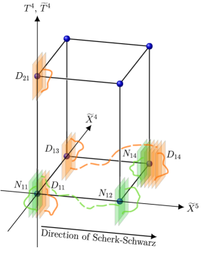
(a) Bosonic states in the NN and DD sectors are massless when their ends are attached to the same stack of branes. By contrast, fermionic states in the NN and DD sectors are massless when they are realized as strings stretched between corners of the six-dimensional boxes that are facing each other along the T-dual Scherk–Schwarz direction.

(b) Massless bosonic states in the ND+DN sector are symbolized as strings attached to stacks of D3-branes T-dual to D9-branes and D5-branes that are located at corners having the same coordinates $\tilde{X}^{4}$ and $\tilde{X}^{5}$. For the massless fermionic states in the ND+DN sector, the corners have same coordinate $\tilde{X}^{4}$ and distinct coordinate $\tilde{X}^{5}$.

Figure 2: Visualization of the massless open-string states in the D3-brane pictures. The scalars are depicted as solid lines and the fermions as dashed lines.

To proceed the same way for the fermions, it is convenient to define a new double-primed index $i^{\prime\prime}\in\{1,2\}$ and write $i^{\prime}=2i^{\prime\prime}$ or $2i^{\prime\prime}-1$. The massless fermionic degrees of freedom extracted from $Z_{\cal A}+Z_{\cal M}$ are then identified as the low-lying modes of the following characters,

$${1\over\eta^{8}}\sum_{i,i^{\prime\prime}}\bigg{\{}C_{4}C_{4}\left[n_{i,2i^{\prime\prime}-1}\bar{n}_{i,2i^{\prime\prime}}+\bar{n}_{i,2i^{\prime\prime}-1}n_{i,2i^{\prime\prime}}+d_{i,2i^{\prime\prime}-1}\bar{d}_{i,2i^{\prime\prime}}+\bar{d}_{i,2i^{\prime\prime}-1}d_{i,2i^{\prime\prime}}\right]$$ (2.25)

$$+S_{4}S_{4}\left[n_{i,2i^{\prime\prime}-1}n_{i,2i^{\prime\prime}}+\bar{n}_{i,2i^{\prime\prime}-1}\bar{n}_{i,2i^{\prime\prime}}+d_{i,2i^{\prime\prime}-1}d_{i,2i^{\prime\prime}}+\bar{d}_{i,2i^{\prime\prime}-1}\bar{d}_{i,2i^{\prime\prime}}\right]$$

$$+S_{4}O_{4}\sum_{j}\bigg{[}\frac{1-e^{4i\pi\vec{a}_{i}\cdot\vec{a}_{j}}}{2}\left(n_{i,2i^{\prime\prime}-1}d_{j,2i^{\prime\prime}}+\bar{n}_{i,2i^{\prime\prime}-1}\bar{d}_{j,2i^{\prime\prime}}+n_{i,2i^{\prime\prime}}d_{j,2i^{\prime\prime}-1}+\bar{n}_{i,2i^{\prime\prime}}\bar{d}_{j,2i^{\prime\prime}-1}\right)$$

$$\hskip 28.45274pt+\frac{1+e^{4i\pi\vec{a}_{i}\cdot\vec{a}_{j}}}{2}\left(n_{i,2i^{\prime\prime}-1}\bar{d}_{j,2i^{\prime\prime}}+\bar{n}_{i,2i^{\prime\prime}-1}d_{j,2i^{\prime\prime}}+n_{i,2i^{\prime\prime}}\bar{d}_{j,2i^{\prime\prime}-1}+\bar{n}_{i,2i^{\prime\prime}}d_{j,2i^{\prime\prime}-1}\right)\bigg{]}\bigg{\}}\,.$$

They all correspond to fermionic parts of hypermultiplets in fundamental $\otimes$ fundamental or fundamental $\otimes$ $\overline{\text{fundamental}}$ representations of pairs of unitary groups supported by stacks of D3-branes (in the T-dual pictures) located at corners with distinct coordinates along the SSdirection $\tilde{X}^{5}$ (and possibly distinct positions in $T^{4}/\mathbb{Z}_{2}$ or $\tilde{T}^{4}/\mathbb{Z}_{2}$ in the ND+DN sector). They appear as strings drawn in dashed lines in Fig. 2: Green and orange for the NN and DD sectors in Fig. 2(a), and khaki for the ND+DN sector in Fig. 2(b). Actually, massless fermions are realized as string stretched along the $\tilde{X}^{5}$ direction, translating the fact that the shifts of $m^{\prime}_{5}$ arising from the Wilson lines and the SSmechanism compensate each other (see Eq. (2.6)).

Because the closed-string spectrum is neutral with respect to the gauge group generated by the open strings, it is independent of the deformations $\vec{a}_{i}$ and $\vec{a}_{i^{\prime}}$. As a result, all fermions initially massless in the parent supersymmetric model of Sect. 2.1 acquire tree-level masses equal to $M_{3/2}$ thanks to the SSmechanism. At the massless level, we are left with bosons, which are easily listed from a six-dimensional point of view. The untwisted sector contains the components $(G+C)_{\hat{\mu}\hat{\nu}}$, $\hat{\mu},\hat{\nu}\in\{2,\dots,5\}$, and the internal components $(G+C)_{IJ}$, which yield $(6-2)\times(6-2)+4\times 4$ degrees of freedom. Moreover, there are $4\times 16$ real scalars arising from the twisted hypermultiplets.

3 Two-point functions of massless ND and DN states

In Ref. [32] the masses at one loop of the open-string moduli arising from the NN and DD sectors were derived by using the background field method. However, in the case of the moduli in the ND+DN sector, the partition function for arbitrary vev’s of these scalars is not known and this approach cannot be applied. Therefore, we will derive in Sects. 5 and 6 the one-loop masses of all classically massless scalars in the bifundamental representations of unitary groups supported by D9- and D5-branes by computing two-point correlation functions with external states in the massless ND and DN bosonic sectors. This will be done by applying techniques first introduced in classical open-string theories in Refs. [9, 10, 11], and at one loop in Refs. [13, 14, 15, 16, 17]. For now, we define the relevant vertex operators and open-string amplitudes.

3.1 Vertex operators and amplitudes

In the T-dual pictures, let us consider two corners $i_{0}i_{0}^{\prime}$ and $j_{0}i_{0}^{\prime}$ on which are located $N_{i_{0}i_{0}^{\prime}}\geq 2$ and $D_{j_{0}i_{0}^{\prime}}\geq 2$ D3-branes T-dual to D9-branes and D5-branes, respectively. As seen in the third line of Eq. (LABEL:massless_bosons), the open strings “stretched” between these stacks give rise to $2n_{i_{0}i_{0}^{\prime}}d_{j_{0}j_{0}^{\prime}}$ massless complex scalars (depicted as solid strings in Fig. 2(b)). In the initial description in terms of D9- and D5-branes, we are interested in correlation functions of vertex operators in ghost pictures $p$ and $-p$ of the form

$$\sum_{\alpha_{0}=1}^{N_{i_{0}i_{0}^{\prime}}}\sum_{\beta_{0}=1}^{D_{j_{0}i_{0}^{\prime}}}\left\langle V^{\alpha_{0}\beta_{0}}_{p}(z_{1},k,\epsilon)V^{\beta_{0}\alpha_{0}}_{-p}(z_{2},-k,-\epsilon)\right\rangle^{\Sigma}\,,$$ (3.26)

where $z_{1}$, $z_{2}$ are insertion points on the boundary of a worldsheet whose topology is either that of the annulus or Möbius strip, $\Sigma\in\{{\cal A},{\cal M}\}$, and

$$V_{-1}^{\alpha_{0}\beta_{0}}(z_{1},k,\epsilon) =\lambda_{\alpha_{0}\beta_{0}}\,e^{-\phi}\,e^{ik\cdot X}\,e^{\epsilon{i\over 2}(H_{3}-H_{4})}\,\sigma^{3}\sigma^{4}(z_{1})\,,$$ (3.27)

$$V_{-1}^{\beta_{0}\alpha_{0}}(z_{2},-k,-\epsilon) =\lambda^{\rm T}_{\beta_{0}\alpha_{0}}\,e^{-\phi}\,e^{-ik\cdot X}\,e^{-\epsilon{i\over 2}(H_{3}-H_{4})}\,\sigma^{3}\sigma^{4}(z_{2})\,.$$

In the above definitions, we use the following notations:

• $k^{\mu}$ is the external momentum satisfying on-shell the condition $k^{\mu}k_{\mu}=0$.

• $\phi(z)$ is the ghost field encountered in the bosonization of the superconformal ghosts [60].

• $\lambda$ is the matrix

  $$\lambda=\begin{pmatrix}\Lambda_{1}&\Lambda_{2}\\ -\Lambda_{2}&\Lambda_{1}\end{pmatrix},$$ (3.28)

  where $\Lambda_{1}$, $\Lambda_{2}$ are arbitrary $n_{i_{0}i_{0}^{\prime}}\times d_{j_{0}i_{0}^{\prime}}$ real matrices [4]. It labels the states that transform as the $(n_{i_{0}i_{0}^{\prime}},d_{j_{0}i_{0}^{\prime}})\oplus(\bar{n}_{i_{0}i_{0}^{\prime}},\bar{d}_{j_{0}i_{0}^{\prime}})$ or $(n_{i_{0}i_{0}^{\prime}},\bar{d}_{j_{0}i_{0}^{\prime}})\oplus(\bar{n}_{i_{0}i_{0}^{\prime}},d_{j_{0}i_{0}^{\prime}})$ bifundamental representation of $U(n_{i_{0}i_{0}^{\prime}})\times U(d_{j_{0}i_{0}^{\prime}})$.

• From now until Sect. 6, we restrict our analysis to the case where the internal metric is diagonal,

  $$G_{I^{\prime}J^{\prime}}\equiv\delta_{I^{\prime}J^{\prime}}\,{R_{I^{\prime}}^{2}\over\alpha^{\prime}}\,,\quad\leavevmode\nobreak\ \leavevmode\nobreak\ G_{IJ}\equiv\delta_{IJ}\,{R_{I}^{2}\over\alpha^{\prime}}\,,$$ (3.29)

  for some radii $R_{I^{\prime}}$, $R_{I}$. In this case, the formalism of Ref. [2] applies without having to generalize it. Denoting $\psi^{\mu}(z)$, $\psi^{I^{\prime}}(z)$, $\psi^{I}(z)$ the Grassmann fields superpartners of the bosonic-coordinate fields $X^{\mu}(z)$, $X^{I^{\prime}}(z)$, $X^{I}(z)$, we define a new basis of degrees of freedom

  $${Z}^{u}\equiv\frac{X^{2u}+iX^{2u+1}}{\sqrt{2}}\,, \mkern 1.5mu\overline{\mkern-1.5muZ\mkern-1.5mu}\mkern 1.5mu^{u}\equiv\frac{X^{2u}-iX^{2u+1}}{\sqrt{2}}\,,$$ (3.30)

  $${\Psi}^{u}\equiv\frac{\psi^{2u}+i\psi^{2u+1}}{\sqrt{2}}\equiv e^{iH_{u}}\,, \mkern 1.5mu\overline{\mkern-1.5mu\Psi\mkern-1.5mu}\mkern 1.5mu^{u}\equiv\frac{\psi^{2u}-i\psi^{2u+1}}{\sqrt{2}}\equiv e^{-iH_{u}}\,,\quad u\in\{0,\dots,4\}\,,$$

  where $H_{u}$ are scalars introduced to bosonize the fermionic fields.

• The characters $O_{4}C_{4}$ tell us that the scalars we are interested in are organized as singlet from a six-dimensional point of view, and spinors of the $T^{4}/\mathbb{Z}_{2}$ orbifold space. The operators $e^{\pm\epsilon i(H_{3}-H_{4})}$ are therefore spin fields, which means that the coefficients of $H_{3}$, $H_{4}$ in the exponentials are the weights of the dimension-two spinorial representation of negative chirality of $SO(4)$, which are $\epsilon(\frac{1}{2},-\frac{1}{2})$, $\epsilon\in\{-1,+1\}$.

• $\sigma^{u}$, $u\in\{3,4\}$, are so-called “boundary-changing fields” associated with the complex directions $Z^{u}$ [6].

To understand the meaning and necessity of introducing operators $\sigma^{u}$, the open-string diagrams we want to compute are displayed in Fig. 3 for some given $\alpha_{0}\in\{1,\dots,N_{i_{0}i_{0}^{\prime}}\}$ and $\beta_{0}\in\{1,\dots,D_{j_{0}i_{0}^{\prime}}\}$. The left panel shows two annuli and one Möbius strip amplitudes. Because the external legs bring quantum numbers $(\lambda_{\alpha_{0}\beta_{0}},\epsilon)$ and $(\lambda^{\rm T}_{\beta_{0}\alpha_{0}},-\epsilon)$ of the ND and DN sectors, they must be attached to the same boundary of the annulus. Therefore, the second boundary is sticked to another brane labelled $\gamma$, which can be any of the 32 D9-branes (in green) or 32 D5-branes (in orange). On the center and right panels, the same three diagrams are displayed, with the open-string worldsheets seen as fundamental domains of the involution

$$z\,\longrightarrow\,{\cal I}(z)\equiv 1-\bar{z}$$ (3.31)

acting on double-cover tori of Teichmüller parameters [7, 8, 61, 58]

$$\tau^{\rm dc}=i{\tau_{2}\over 2}\leavevmode\nobreak\ \leavevmode\nobreak\ \mbox{for the annulus}\quad\leavevmode\nobreak\ \leavevmode\nobreak\ \mbox{and}\leavevmode\nobreak\ \leavevmode\nobreak\ \quad\tau^{\rm dc}=\frac{1}{2}+i{\tau_{2}\over 2}\leavevmode\nobreak\ \leavevmode\nobreak\ \mbox{for the M\"{o}bius strip}\,.$$ (3.32)

In this description, the external legs are conformally mapped to points $z_{1}$, $z_{2}$, where vertex operators change the boundary conditions of the worldsheet fields $X^{I}(z)$ (i.e. $Z^{3}(z)$, $Z^{4}(z)$)

     

     

​​​  ​​​​​​​​​​​​ ​​​​​​​​​

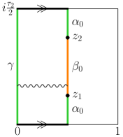
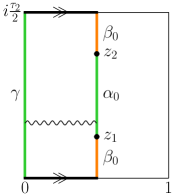
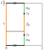
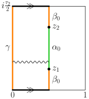
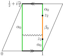
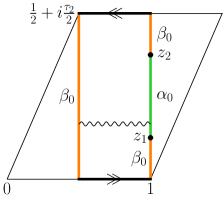
Figure 3: Open-string diagrams with two external legs in the ND and DN sectors (left panel). On the double-cover tori (center and right panels), the external legs are mapped to boundary-changing vertex operators at $z_{1}$, $z_{2}$. One switches from center to right panel by transporting $z_{2}$ along the entire edge it belongs to.

at one end of the intermediate open string running in the loop, from Neumann to Dirichlet or vice versa. The diagrams in the center and right panels are obtained from one another by transporting continuously $z_{2}$ along its entire boundary: $z_{2}\to z_{2}+i\,{\rm Im}\,\tau^{\rm dc}$ for the annulus and $z_{2}\to z_{2}+2i\,{\rm Im}\,\tau^{\rm dc}$ for the Möbius strip, modulo 1 and $\tau^{\rm dc}$.

To conclude this subsection, notice that for consistency of the diagrams, the numbers of boundary-changing vertex operators must be even on each connected component of an open-string surface. Hence, all one-point functions i.e. tadpoles of states in the ND or DN sectors vanish, which shows that the backgrounds we consider, i.e. where no brane recombination is taking place [46, 47, 48, 49], imply the effective potential to be extremal with respect to the scalars in the ND+DN sector.

3.2 OPE’s and ghost-picture changing

In order to treat symmetrically both vertex operators when computing the correlation functions (3.26), we switch to the ghost picture $p=0$. This is done by applying the formula

$$V_{0}^{\alpha_{0}\beta_{0}}(z,k,\epsilon) =\lim_{w\rightarrow z}e^{\phi}\,T_{\text{F}}(w)\,V^{\alpha_{0}\beta_{0}}_{-1}(z,k,\epsilon)\,,$$ (3.33)

$$V_{0}^{\beta_{0}\alpha_{0}}(z,-k,-\epsilon) =\lim_{w\rightarrow z}e^{\phi}\,T_{\text{F}}(w)\,V^{\beta_{0}\alpha_{0}}_{-1}(z,-k,-\epsilon)\,,$$

where $T_{\rm F}$ is the supercurrent given by

$$\begin{split}T_{\text{F}}(z)=\frac{1}{\sqrt{\alpha^{\prime}}}\,\partial X^{\mu}\psi_{\mu}(z)=\frac{1}{\sqrt{\alpha^{\prime}}}\big{(}\partial\mkern 1.5mu\overline{\mkern-1.5muZ\mkern-1.5mu}\mkern 1.5mu^{u}\Psi^{u}(z)+\partial Z^{u}\mkern 1.5mu\overline{\mkern-1.5mu\Psi\mkern-1.5mu}\mkern 1.5mu^{u}(z)\big{)}\,.\end{split}$$ (3.34)

To this end, we display all necessary operator product expansions (OPE’s). First of all, for the “ground-state boundary-changing fields”, we have

$$\begin{split}&\partial Z^{u}(z)\sigma^{u}(w)\underset{z\to w}{\sim}(z-w)^{-\frac{1}{2}}\,\tau^{u}(w)+\mbox{finite}\,,\\ &\partial\mkern 1.5mu\overline{\mkern-1.5muZ\mkern-1.5mu}\mkern 1.5mu^{u}(z)\sigma^{u}(w)\underset{z\to w}{\sim}(z-w)^{-\frac{1}{2}}\,\tau^{\prime u}(w)+\mbox{finite}\,,\end{split}$$ (3.35)

which introduces “excited boundary-changing fields” $\tau^{u}$, $\tau^{\prime u}$. Moreover, the other fields satisfy [13, 14]

$$e^{a\phi}(z)e^{b\phi}(w) \underset{z\to w}{\sim}(z-w)^{-ab}\,e^{(a+b)\phi}(w)+\mbox{finite}\,,$$

$$e^{iaH_{u}}(z)e^{ibH_{u}}(w) \underset{z\to w}{\sim}(z-w)^{ab}\,e^{i(a+b)H_{u}}(w)+\mbox{finite}\,,\quad u\in\{3,4\}\,,$$ (3.36)

$$\partial Z^{u}(z)\,e^{ik\cdot X}(w) \underset{z\to w}{\sim}{iK^{u}\over z-w}\,e^{ik\cdot X}(w)+\mbox{finite}\,,\quad\mbox{where}\quad K^{u}={k^{2u}+ik^{2u+1}\over\sqrt{2}}\,,$$

$$\partial\mkern 1.5mu\overline{\mkern-1.5muZ\mkern-1.5mu}\mkern 1.5mu^{u}(z)\,e^{ik\cdot X}(w) \underset{z\to w}{\sim}{i\mkern 1.5mu\overline{\mkern-1.5muK\mkern-1.5mu}\mkern 1.5mu^{u}\over z-w}\,e^{ik\cdot X}(w)+\mbox{finite}\,,\quad\mbox{where}\quad\mkern 1.5mu\overline{\mkern-1.5muK\mkern-1.5mu}\mkern 1.5mu^{u}={k^{2u}-ik^{2u+1}\over\sqrt{2}}\,,\quad u\in\{0,1,2\}\,.$$

Using these relations, we obtain for $\epsilon=+1$

$$V_{0}^{\alpha_{0}\beta_{0}}(z_{1},k,+1) =V_{0,\rm ext}^{\alpha_{0}\beta_{0}}(z_{1},k,+1)+V_{0,\rm int}^{\alpha_{0}\beta_{0}}(z_{1},k,+1)\,,$$ (3.37)

$$V_{0}^{\beta_{0}\alpha_{0}}(z_{2},-k,-1) =V_{0,\rm ext}^{\beta_{0}\alpha_{0}}(z_{1},-k,-1)+V_{0,\rm int}^{\beta_{0}\alpha_{0}}(z_{1},-k,-1)\,,$$

where we have defined

$$V_{0,\rm ext}^{\alpha_{0}\beta_{0}}(z_{1},k,+1) =\sqrt{\alpha^{\prime}}\,\lambda_{\alpha_{0}\beta_{0}}\,e^{ik\cdot X}\,i\sum_{u=0}^{1}(K^{u}\mkern 1.5mu\overline{\mkern-1.5mu\Psi\mkern-1.5mu}\mkern 1.5mu^{u}+\bar{K}^{u}\Psi^{u})\,e^{\frac{i}{2}(H_{3}-H_{4})}\,\sigma^{3}\sigma^{4}(z_{1})\,,$$ (3.38)

$$V_{0,\rm int}^{\alpha_{0}\beta_{0}}(z_{1},k,+1) ={\lambda_{\alpha_{0}\beta_{0}}\over\sqrt{\alpha^{\prime}}}\,e^{ik\cdot X}\Big{(}e^{-\frac{i}{2}(H_{3}+H_{4})}\,\tau^{3}\sigma^{4}(z_{1})+e^{\frac{i}{2}(H_{3}+H_{4})}\,\sigma^{3}\tau^{\prime 4}(z_{1})\Big{)}\,,$$

$$V_{0,\rm ext}^{\beta_{0}\alpha_{0}}(z_{2},-k,-1) =\sqrt{\alpha^{\prime}}\,\lambda^{\rm T}_{\beta_{0}\alpha_{0}}\,e^{-ik\cdot X}\,(-i)\sum_{u=0}^{1}(K^{u}\mkern 1.5mu\overline{\mkern-1.5mu\Psi\mkern-1.5mu}\mkern 1.5mu^{u}+\bar{K}^{u}\Psi^{u})\,e^{-\frac{i}{2}(H_{3}-H_{4})}\,\sigma^{3}\sigma^{4}(z_{2})\,,$$

$$V_{0,\rm int}^{\beta_{0}\alpha_{0}}(z_{2},-k,-1) ={\lambda^{\rm T}_{\beta_{0}\alpha_{0}}\over\sqrt{\alpha^{\prime}}}\,e^{-ik\cdot X}\Big{(}e^{-\frac{i}{2}(H_{3}+H_{4})}\,\sigma^{3}\tau^{4}(z_{2})+e^{\frac{i}{2}(H_{3}+H_{4})}\,\tau^{\prime 3}\sigma^{4}(z_{2})\Big{)}\,,$$

while the expressions for $\epsilon=-1$ are obtained by exchanging all subscripts and superscripts 3 and 4. Because we are interested in states massless at tree level, the Kaluza–Klein momentum in the $T^{2}$ complex direction $u=2$ is set to 0 in the “external” parts of the vertex operators. In the “internal” parts, notice the appearance of “excited boundary-changing operators” $\tau^{3},\tau^{\prime 3},\tau^{4},\tau^{\prime 4}$.

Given the above definitions, the correlation functions (3.26) split accordingly into external and internal pieces. The former,

$$\!\!\!\!A_{\text{ext}\Sigma}^{\alpha_{0}\beta_{0}} \equiv\big{\langle}V_{0,\rm ext}^{\alpha_{0}\beta_{0}}(z_{1},k,+1)V_{0,\rm ext}^{\beta_{0}\alpha_{0}}(z_{2},-k,-1)\big{\rangle}^{\Sigma}$$ (3.39)

$$=\alpha^{\prime}\,\lambda_{\alpha_{0}\beta_{0}}\lambda^{\rm T}_{\beta_{0}\alpha_{0}}\,\langle e^{ik\cdot X}(z_{1})e^{-ik\cdot X}(z_{2})\rangle\,\langle e^{\frac{i}{2}H_{3}}(z_{1})e^{-\frac{i}{2}H_{3}}(z_{2})\rangle\,\langle e^{-\frac{i}{2}H_{4}}(z_{1})e^{\frac{i}{2}H_{4}}(z_{2})\rangle\times\phantom{\!\!\overset{\displaystyle|}{|}}$$

$$\!\!\!\!\!\!\!\langle\sigma^{3}(z_{1})\sigma^{3}(z_{2})\rangle\,\langle\sigma^{4}(z_{1})\sigma^{4}(z_{2})\rangle\sum_{u=0}^{1}K^{u}\mkern 1.5mu\overline{\mkern-1.5muK\mkern-1.5mu}\mkern 1.5mu^{u}\Big{[}\langle e^{iH_{u}}(z_{1})e^{-iH_{u}}(z_{2})\rangle+\langle e^{-iH_{u}}(z_{1})e^{iH_{u}}(z_{2})\rangle\Big{]}\,,$$

are useful to derive the one-loop corrections to the Kähler potential of the ND+DN sector massless scalars. Note that in order to bypass the issue that on shell $\sum_{u=0}^{1}|K^{u}|^{2}\equiv k^{2}/2=0$, we may have kept the Kaluza–Klein momenta along $T^{2}$ arbitrary. On the contrary, the internal parts,

$$A_{\text{int}\Sigma}^{\alpha_{0}\beta_{0}} \equiv\big{\langle}V_{0,\rm int}^{\alpha_{0}\beta_{0}}(z_{1},k,+1)V_{0,\rm int}^{\beta_{0}\alpha_{0}}(z_{2},-k,-1)\big{\rangle}^{\Sigma}$$ (3.40)

$$=\frac{1}{\alpha^{\prime}}\,\lambda_{\alpha_{0}\beta_{0}}\lambda^{\rm T}_{\beta_{0}\alpha_{0}}\,\langle e^{ik\cdot X}(z_{1})e^{-ik\cdot X}(z_{2})\rangle\phantom{\!\!\overset{\displaystyle|}{|}}$$

$$\leavevmode\nobreak\ \leavevmode\nobreak\ \leavevmode\nobreak\ \times\Big{[}\langle e^{-\frac{i}{2}H_{3}}(z_{1})e^{\frac{i}{2}H_{3}}(z_{2})\rangle\,\langle e^{-\frac{i}{2}H_{4}}(z_{1})e^{\frac{i}{2}H_{4}}(z_{2})\rangle\,\langle\tau^{3}(z_{1})\tau^{\prime 3}(z_{2})\rangle\,\langle\sigma^{4}(z_{1})\sigma^{4}(z_{2})\rangle$$

$$\leavevmode\nobreak\ \leavevmode\nobreak\ \leavevmode\nobreak\ \leavevmode\nobreak\ \,+\langle e^{\frac{i}{2}H_{3}}(z_{1})e^{-\frac{i}{2}H_{3}}(z_{2})\rangle\,\langle e^{\frac{i}{2}H_{4}}(z_{1})e^{-\frac{i}{2}H_{4}}(z_{2})\rangle\,\langle\sigma^{3}(z_{1})\sigma^{3}(z_{2})\rangle\,\langle\tau^{\prime 4}(z_{1})\tau^{4}(z_{2})\rangle\Big{]}\,,$$

capture the mass corrections we are interested in. The amplitudes for $\epsilon=-1$ are obtained by exchanging all subscripts 3 and 4 in Eq. (3.39) and all superscripts 3 and 4 in Eq. (3.40). For $\Sigma={\cal A}$, an implicit sum over a second boundary condition $\gamma$ is understood. Likewise, for $\Sigma={\cal A}$, ${\cal M}$, sums over the spin structures of the fermions $\Psi^{0}$, $\Psi^{1}$, $\Psi^{2}$ on the one hand, and $\Psi^{3}$, $\Psi^{4}$ on the other hand are implicit.

4 Genus-1 twist-field correlation functions

The main difficulty in computing the two-point functions in Eqs. (3.39) and (3.40) is to evaluate the correlators of the boundary changing operators. However, it turns out that the OPE’s of $\partial Z^{u}$, $\partial\mkern 1.5mu\overline{\mkern-1.5muZ\mkern-1.5mu}\mkern 1.5mu^{u}$ on these operators are identical to those found for the holomorphic part of “$\mathbb{Z}_{2}$-twist fields” inserted on a closed-string worldsheet, i.e. for operators creating closed strings in the twisted sector of a $T^{4}/\mathbb{Z}_{2}$ orbifold. As a result, we may apply techniques relevant for the computation of correlation functions of twist fields in closed-string theory to our open-string case. In the present section, we review the relevant ingredients for computing correlators of twist fields at genus-1 in closed-string theory, or in the closed-string sector of an open-string theory, compactified on toroidal $\mathbb{Z}_{N}$ orbifolds, following the original works of Refs. [2, 1].

4.1 Instanton decomposition of correlators

In closed-string theory compactified on $T^{2}\times T^{4}/\mathbb{Z}_{N}$ where $N\in\mathbb{N}^{*}$, the complex fields defined in Eq. (3.30) depend on holomorphic and antiholomorphic worldsheet coordinates, $Z^{u}(z,\bar{z})$. Moreover, upon parallel transport, the internal $Z^{u}$ undergo some $\mathbb{Z}_{N}$ rotations and translations,

$$Z^{2} \,\longrightarrow\,Z^{2}+v^{2}\,,$$ (4.41)

$$Z^{u} \,\longrightarrow\,e^{2i\pi{\kappa/N}}Z^{u}+v^{u}\,,\quad u\in\{3,4\}\,,\leavevmode\nobreak\ \leavevmode\nobreak\ \kappa\in\{0,\dots,N-1\}\,,$$

where the shifts $v^{u}$ and $v^{2}$ implement the $T^{4}$ and $T^{2}$ periodicities.

The twist fields create the states in the twisted sectors of the closed-string Hilbert space. For some given $\kappa\in\{1,\dots,N-1\}$ and $u\in\{3,4\}$, let us denote by $\sigma^{u}(z,\bar{z})$ the one that creates the ground state in the $\kappa$-th twisted sector. The requirement that positive frequency modes in the expansions of $\partial Z^{u}$ and $\partial\mkern 1.5mu\overline{\mkern-1.5muZ\mkern-1.5mu}\mkern 1.5mu^{u}$ annihilate the twisted ground state determines the OPE of $\partial Z^{u}(z)$ and $\partial\mkern 1.5mu\overline{\mkern-1.5muZ\mkern-1.5mu}\mkern 1.5mu^{u}(z)$ acting on $\sigma^{u}(w,\bar{w})$ as $z$ approaches $w$,

$$\partial Z^{u}(z)\sigma^{u}(w,\bar{w})\underset{z\to w}{\sim}(z-w)^{-(1-\kappa/N)}\,\tau^{u}(w,\bar{w}) \!\!\!\!\!+\mbox{finite}\,,$$ (4.42)

$$\partial\mkern 1.5mu\overline{\mkern-1.5muZ\mkern-1.5mu}\mkern 1.5mu^{u}(z)\sigma^{u}(w,\bar{w})\underset{z\to w}{\sim}(z-w)^{-\kappa/N}\,\tau^{\prime u}(w,\bar{w}) \!\!\!\!\!+\mbox{finite}\,,$$

$$\bar{\partial}Z^{u}(\bar{z})\sigma^{u}(w,\bar{w})\underset{\bar{z}\to\bar{w}}{\sim}(\bar{z}-\bar{w})^{-\kappa/N}\,\tilde{\tau}^{u}(w,\bar{w}) \!\!\!\!\!+\mbox{finite}\,,$$

$$\bar{\partial}\mkern 1.5mu\overline{\mkern-1.5muZ\mkern-1.5mu}\mkern 1.5mu^{u}(\bar{z})\sigma^{u}(w,\bar{w})\underset{\bar{z}\to\bar{w}}{\sim}(\bar{z}-\bar{w})^{-(1-\kappa/N)}\,\tilde{\tau}^{\prime u}(w,\bar{w}) \!\!\!\!\!+\mbox{finite}\,.$$

In the right-hand sides, $\tau^{u}$, $\tau^{\prime u}$, $\tilde{\tau}^{u}$, $\tilde{\tau}^{\prime u}$ create excited states in the $\kappa$-th twisted sector. The OPE’s capture the local behavior corresponding to the rotations of the coordinates $Z^{u}$ but do not carry information about the global translations $v^{u}$. This data is recovered by imposing global monodromy conditions which describe how $Z^{u}(z,\bar{z})$ and $\mkern 1.5mu\overline{\mkern-1.5muZ\mkern-1.5mu}\mkern 1.5mu^{u}(z,\bar{z})$ change when they are carried around a set of twist fields with vanishing total twist. Splitting the coordinates of $T^{2}$ and $T^{4}$ into background values and quantum fluctuations,

$$Z^{u}(z,\bar{z})=Z_{\text{cl}}^{u}(z,\bar{z})+Z_{\text{qu}}^{u}(z,\bar{z})\,,\quad u\in\{2,3,4\}\,,$$ (4.43)

the whole global displacements arise from the classical parts $Z_{\text{cl}}^{u}(z,\bar{z})$.

With this decomposition, the correlators of interest on a Riemann surface $\Sigma$ of genus $g\geq 0$ involve, for each complex direction $u\in\{3,4\}$, $L\geq 2$ ground-state twist fields $\sigma_{A}^{u}$ of the $\kappa_{A}$-th twisted sector,

$$\sum_{Z_{\text{cl}}}e^{-S_{\text{cl}}^{\Sigma}}\prod_{u=3}^{4}\left\langle\prod_{A=1}^{L}\sigma_{A}^{u}(z_{A},\bar{z}_{A})\right\rangle_{\text{qu}},$$ (4.44)

where the total twist is trivial, $\sum_{A}\kappa_{A}=0$ modulo $N$, for the result not to vanish [1]. In this expression, the sum is over instantons with worldsheet actions

$$S_{\text{cl}}^{\Sigma}=\frac{i}{2\pi\alpha^{\prime}}\int_{\Sigma}\text{d}z\wedge\text{d}\bar{z}\,\sum_{u=2}^{4}\big{(}\partial Z_{\text{cl}}^{u}\,\bar{\partial}\mkern 1.5mu\overline{\mkern-1.5muZ\mkern-1.5mu}\mkern 1.5mu_{\text{cl}}^{u}+\partial\mkern 1.5mu\overline{\mkern-1.5muZ\mkern-1.5mu}\mkern 1.5mu_{\text{cl}}^{u}\,\bar{\partial}Z_{\text{cl}}^{u}\big{)}\,.$$ (4.45)

In the following, we first compute the “quantum parts” of the correlation functions and then derive the classical actions.

4.2 Stress-tensor method

To determine for a given $u\in\{3,4\}$ the quantum part $\left\langle\prod_{A=1}^{L}\sigma_{A}^{u}(z_{A},\bar{z}_{A})\right\rangle_{\text{qu}}$ of the correlator (4.44), Ref. [2] uses the stress-tensor method. It consists in exploiting the OPE’s between the stress tensor $T^{u}(z)$ and the primary fields $\sigma_{A}^{u}(z_{A},\bar{z}_{A})$ of conformal weights $h_{A}=\frac{1}{2}(\kappa_{A}/N)(1-\kappa_{A}/N)$, namely

$$T^{u}(z)\sigma_{A}^{u}(z_{A},\bar{z}_{A})\underset{z\to z_{A}}{\sim}\frac{h_{A}}{(z-z_{A})^{2}}\,\sigma_{A}^{u}(z_{A},\bar{z}_{A})+\frac{1}{z-z_{A}}\,\partial_{A}\sigma_{A}^{u}(z_{A},\bar{z}_{A})+\mbox{finite}\,.$$ (4.46)

To this end, one considers the quantity

$$\langle\langle T^{u}(z)\rangle\rangle\equiv\frac{\left\langle T^{u}(z)\prod_{A}\sigma^{u}_{A}(z_{A},\bar{z}_{A})\right\rangle_{\rm qu}}{\left\langle\prod_{A}\sigma^{u}_{A}(z_{A},\bar{z}_{A})\right\rangle_{\rm qu}}\,,$$ (4.47)

in terms of which we may write

$$\partial_{B}\ln\big{\langle}\prod_{A}\sigma^{u}_{A}(z_{A},\bar{z}_{A})\big{\rangle}_{\rm qu}=\lim_{z\rightarrow z_{B}}\left[(z-z_{B})\,\langle\langle T^{u}(z)\rangle\rangle-\frac{h_{B}}{(z-z_{B})}\right],$$ (4.48)

upon using Eq. (4.46). To evaluate $\langle\langle T^{u}(z)\rangle\rangle$, one considers the Green’s function in the presence of twist fields,

$$g(z,w)\equiv\frac{\langle-\partial Z^{u}_{\rm qu}(z)\,\partial\mkern 1.5mu\overline{\mkern-1.5muZ\mkern-1.5mu}\mkern 1.5mu^{u}_{\rm qu}(w)\prod_{A}\sigma^{u}_{A}(z_{A},\bar{z}_{A})\rangle_{\rm qu}}{\alpha^{\prime}\,\langle\prod_{A}\sigma^{u}_{A}(z_{A},\bar{z}_{A})\rangle_{\rm qu}}\,,$$ (4.49)

and exploits the OPE

$$-{1\over\alpha^{\prime}}\,\partial Z^{u}_{\rm qu}(z)\,\partial\mkern 1.5mu\overline{\mkern-1.5muZ\mkern-1.5mu}\mkern 1.5mu^{u}_{\rm qu}(w)\underset{z\to w}{\sim}\frac{1}{(z-w)^{2}}+T^{u}(w)+{\cal O}(z-w)$$ (4.50)

to obtain

$$\langle\langle T^{u}(z)\rangle\rangle=\lim_{w\rightarrow z}\left[g(z,w)-\frac{1}{(z-w)^{2}}\right].$$ (4.51)

To summarise, the stress-tensor method amounts to determining the Green’s function $g(z,w)$, then deduce $\langle\langle T^{u}(z)\rangle\rangle$, and finally integrate the differential equations (4.48).

4.3 Ground-state twist field quantum correlators on the torus

Let us specialize to the case where $\Sigma$ is a genus-1 surface. We will denote its Teichmüller parameter as $\tau^{\rm dc}$ for future use, when we see the genus-1 Riemann surface as the double cover of open-string surfaces.

In order to derive the quantum part of the correlator (4.44) for a given $u\in\{3,4\}$, $\left\langle\prod_{A=1}^{L}\sigma_{A}^{u}(z_{A},\bar{z}_{A})\right\rangle_{\text{qu}}$, the starting point is to write the most general ansätze for $g(z,w)$ and the companion Green’s function

$$h(\bar{z},w)\equiv\frac{\langle-\bar{\partial}Z^{u}_{\rm qu}(\bar{z})\,\partial\mkern 1.5mu\overline{\mkern-1.5muZ\mkern-1.5mu}\mkern 1.5mu^{u}_{\rm qu}(w)\prod_{A}\sigma^{u}_{A}(z_{A},\bar{z}_{A})\rangle_{\rm qu}}{\alpha^{\prime}\,\langle\prod_{A}\sigma^{u}_{A}(z_{A},\bar{z}_{A})\rangle_{\rm qu}}\,,$$ (4.52)

satisfying the following properties:

• Double periodicity $z\to z+1$, $z\to z+\tau^{\rm dc}$ and $w\to w+1$, $w\to w+\tau^{\rm dc}$ (and similarly for $\bar{z}$ in $h$).

• Local monodromies consistent with the OPE’s given in Eq. (4.42). For instance, when $z$ is transported along a tiny closed loop encircling some $z_{A}$, $g$ must transform as $e^{-2i\pi(1-\kappa_{A}/N)}g$.

• A double pole for $g(z,w)$ as $z\to w$ dictated by Eq. (4.50), and finiteness of $h(\bar{z},w)$ as $\bar{z}\to w$ thanks to the OPE $\bar{\partial}Z^{u}_{\rm qu}(\bar{z})\partial\mkern 1.5mu\overline{\mkern-1.5muZ\mkern-1.5mu}\mkern 1.5mu^{u}_{\rm qu}(w)\underset{\bar{z}\to w}{\sim}\mbox{finite}$.

This can be done by defining cut differentials [2] which form a basis of holomorphic one-forms on the torus that possess suitable monodromy behaviors as their arguments approach each of the insertion points $z_{A}$. Denoting

$$M=\sum_{A=1}^{L}{\kappa_{A}\over N}\,,$$ (4.53)

which takes some value in the set $\{1,\dots,L-1\}$, and following the notations of Ref. [2], such a basis is given by

$$\omega_{N-\kappa}^{\alpha_{A}}(z) =\gamma_{N-\kappa}(z)\,\vartheta_{1}(z-z_{\alpha_{A}}-y_{N-\kappa})\prod_{B\neq A}^{L-M}\vartheta_{1}(z-z_{\alpha_{B}})\,, \,A\in\{1,\dots,L-M\}\,,$$ (4.54)

$$\omega_{\kappa}^{\beta_{A}}(z) =\gamma_{\kappa}(z)\,\vartheta_{1}(z-z_{\beta_{A}}-y_{\kappa})\prod_{B\neq A}^{M}\vartheta_{1}(z-z_{\beta_{B}})\,, \,A\in\{1,\dots,M\}\,,$$

where the second argument at $\tau^{\rm dc}$ in the modular forms is implicit. In these formulas, we have defined the functions

$$\gamma_{N-\kappa}(z)=\prod_{A=1}^{L}\vartheta_{1}(z-z_{A})^{-(1-\kappa_{A}/N)}\,,\leavevmode\nobreak\ \leavevmode\nobreak\ \quad\gamma_{\kappa}(z)=\prod_{A=1}^{L}\vartheta_{1}(z-z_{A})^{-\kappa_{A}/N}\,,$$ (4.55)

and denoted

$$y_{N-\kappa}=\sum_{A=1}^{L}\left(1-\frac{k_{A}}{N}\right)z_{A}-\sum_{B=1}^{L-M}z_{\alpha_{B}}\,,\leavevmode\nobreak\ \leavevmode\nobreak\ \quad y_{\kappa}=\sum_{A=1}^{L}\frac{\kappa_{A}}{N}z_{A}-\sum_{B=1}^{M}z_{\beta_{B}}\,,$$ (4.56)

while $\{z_{\alpha_{1}},\dots,z_{\alpha_{L-M}}\}$ and $\{z_{\beta_{1}},\dots,z_{\beta_{M}}\}$ are subsets of twist insertion points chosen arbitrarily. The functions $\gamma_{N-\kappa}$ and $\gamma_{\kappa}$ implement the monodromies around the $z_{A}$’s, while the extra $\vartheta_{1}$ modular forms in the definitions (4.54) lead to the double periodicity with respect to the variable $z$. Given these notations, the Green’s functions may be expressed as

$$g(z,w) =g_{s}(z,w)+\sum_{A=1}^{L-M}\sum_{B=1}^{M}C_{AB}\,\omega_{N-\kappa}^{\alpha_{A}}(z)\,\omega_{\kappa}^{\beta_{B}}(w)\,,$$ (4.57)

$$h(\bar{z},w) =\sum_{A=1}^{M}\sum_{B=1}^{M}B_{AB}\,\bar{\omega}_{\kappa}^{\beta_{A}}(\bar{z})\,\omega_{\kappa}^{\beta_{B}}(w)\,,$$

where $C_{AB}$ and $B_{AB}$ are “constant coefficients.” The function $g_{s}(z,w)$ is doubly periodic in $z$ and $w$ and handles the double-pole structure of $g(z,w)$ as $z$ approaches $w$. It can be expressed as [2]

$$g_{s}(z,w)=\gamma_{N-\kappa}(z)\,\gamma_{\kappa}(w)\left(\frac{\vartheta_{1}^{\prime}(0)}{\vartheta_{1}(z-w)}\right)^{2}P(z,w)\,,$$ (4.58)

where explicit knowledge of the function $P(z,w)$ is not required in the computation of correlation functions of ground-state twist fields. However, it does matter for correlators of excited twist fields, as will be seen in Sect. 4.5. We will come back to this issue at that stage.

The next step is to implement the global monodromy conditions, which by definition are “trivial” for the quantum fluctuations $Z_{\rm qu}^{u}(z,\bar{z})$ (see below Eq. (4.43)). In practice, this implies that

$$0=\oint_{\gamma_{a}}\text{d}z\,g(z,w)+\oint_{\gamma_{a}}\text{d}\bar{z}\,h(\bar{z},w)\,,\quad a\in\{1,\dots,L\}\,,$$ (4.59)

where $\{\gamma_{a},\ a=1,\dots,L\}$ is a basis of the homology group of the genus-1 surface with $L$ punctures. To solve these equations, it is convenient to define an $L\times L$ cut-period matrix ${W_{a}}^{A}$ as follows,

$${W_{a}}^{A} =\oint_{\gamma_{a}}\text{d}z\,\omega_{N-\kappa}^{\alpha_{A}}(z)\,, A\in\{1,\dots,L-M\}\,,$$ (4.60)

$${W_{a}}^{L-M+A} =\oint_{\gamma_{a}}\text{d}\bar{z}\,\bar{\omega}_{\kappa}^{\beta_{A}}(\bar{z})\,, A\in\{1,\dots,M\}\,.$$

Indeed, it is easily checked that the expressions

$$g(z,w) =g_{s}(z,w)-\sum_{A=1}^{L-M}\omega_{N-\kappa}^{\alpha_{A}}(z)\sum_{a=1}^{L}{(W^{-1})_{A}}^{a}\oint_{\gamma_{a}}\text{d}\zeta\,g_{s}(\zeta,w)\,,$$ (4.61)

$$h(\bar{z},w) =-\sum_{A=1}^{M}\omega_{\kappa}^{\beta_{A}}(\bar{z})\sum_{a=1}^{L}{(W^{-1})_{L-M+A}}^{a}\oint_{\gamma_{a}}\text{d}\zeta\,g_{s}(\zeta,w)\,,$$

satisfy the global monodromy conditions.

Finally, the correlator can be found by applying the stress-tensor method to find the holomorphic dependence on the $z_{A}$’s, and then a second time using the Green’s functions $\bar{g}(\bar{z},\bar{w})$ and $\bar{h}(z,\bar{w})$ to determine the antiholomorphic part. The result is for $u\in\{3,4\}$

$$\left\langle\prod_{A=1}^{L}\sigma_{A}^{u}(z_{A},\bar{z}_{A})\right\rangle_{\text{qu}}= \;f(\tau^{\rm dc};\kappa_{1},\dots,\kappa_{L})\,{1\over\det W}\;\vartheta_{1}(y_{N-\kappa})^{L-M-1}\;\mkern 1.5mu\overline{\mkern-1.5mu\vartheta_{1}(y_{\kappa})\mkern-1.5mu}\mkern 1.5mu^{M-1}$$

$$\times\prod_{\begin{subarray}{c}A,B=1\\ A<B\end{subarray}}^{L-M}\vartheta_{1}(z_{\alpha_{A}}-z_{\alpha_{B}})\,\prod_{\begin{subarray}{c}A,B=1\\ A<B\end{subarray}}^{M}\mkern 1.5mu\overline{\mkern-1.5mu\vartheta_{1}(z_{\beta_{A}}-z_{\beta_{B}})\mkern-1.5mu}\mkern 1.5mu$$ (4.62)

$$\times\prod_{\begin{subarray}{c}A,B=1\\ A<B\end{subarray}}^{L}\vartheta_{1}(z_{A}-z_{B})^{-(1-\kappa_{A}/N)(1-\kappa_{B}/N)}\;\mkern 1.5mu\overline{\mkern-1.5mu\vartheta_{1}(z_{A}-z_{B})\mkern-1.5mu}\mkern 1.5mu^{-(\kappa_{A}/N)(\kappa_{B}/N)}\,,$$

where $f(\tau^{\rm dc},\kappa_{1},\dots,\kappa_{L})$ is a function arising as an “integration constant”. The latter can be determined by coalescing all insertion points, since the left-hand side reduces in this case to $\langle 1\rangle$, which is the partition function.

4.4 Instanton actions

In the OPE’s (4.42), the actions of the background parts $\partial Z_{\text{cl}}^{u}(z)$ and $\partial\mkern 1.5mu\overline{\mkern-1.5muZ\mkern-1.5mu}\mkern 1.5mu_{\rm cl}^{u}(z)$ on $\sigma^{u}(w,\bar{w})$ for $u\in\{3,4\}$ are trivial multiplications. Hence, for the monodomy properties to be satisfied as $z$ is transported along a tiny closed loop encircling any $z_{A}$, the doubly-periodic $\partial Z_{\text{cl}}^{u}(z)$ and $\partial\mkern 1.5mu\overline{\mkern-1.5muZ\mkern-1.5mu}\mkern 1.5mu_{\rm cl}^{u}(z)$ must be linear sums of cut differentials. To determine the coefficients, one imposes the global monodromy conditions

$$\oint_{\gamma_{a}}\text{d}z\,\partial Z_{\text{cl}}^{u}+\oint_{\gamma_{a}}\text{d}\bar{z}\,\bar{\partial}Z_{\text{cl}}^{u}=v^{u}_{a}\,,\quad a\in\{1,\dots,L\}\,,$$ (4.63)

where the $v^{u}_{a}$’s are displacement vectors. The solution of these equations can be expressed in terms of the inverse cut-period matrix,

$$\partial Z_{\text{cl}}^{u}(z)=\omega_{A^{\prime}}(z)\,{(W^{-1})_{A^{\prime}}}^{a}\,v^{u}_{a}\,,\qquad\bar{\partial}Z_{\text{cl}}^{u}(\bar{z})=\bar{\omega}_{A^{\prime\prime}}(\bar{z})\,{(W^{-1})_{A^{\prime\prime}}}^{a}\,v^{u}_{a}\,,$$ (4.64)

where in the present context the index $A^{\prime}$ is summed over $1,\dots,L-M$, and $A^{\prime\prime}$ is summed over $L-M+1,\dots,L$. Moreover, we have redefined in the above formulas

$$\omega_{A}(z) \equiv\omega_{N-\kappa}^{\alpha_{A}}(z)\,, \,A\in\{1,\dots,L-M\}\,,$$ (4.65)

$$\omega_{L-M+A}(z) \equiv\omega_{\kappa}^{\beta_{A}}(z)\,, \,A\in\{1,\dots,M\}\,.$$

With the definition of the Hermitian product

$$(\omega_{i},\omega_{j})\equiv i\int_{\Sigma}\text{d}z\wedge\text{d}\bar{z}\,\omega_{i}(z)\,\bar{\omega}_{j}(\bar{z})$$ (4.66)

of one-forms on the torus, the classical action for a single complex coordinate $u\in\{3,4\}$ reads

$$S_{\text{cl}}^{\Sigma}\big{|}^{u}=\frac{v^{u}_{a}\bar{v}^{u}_{b}}{2\pi\alpha^{\prime}}\Big{[}{(W^{-1})_{A^{\prime}}}^{a}\,{(W^{-1})_{B^{\prime}}}^{b}\,(\omega_{A^{\prime}},\omega_{B^{\prime}})+{(W^{-1})_{A^{\prime\prime}}}^{a}\,{(W^{-1})_{B^{\prime\prime}}}^{b}\,(\omega_{A^{\prime\prime}},\omega_{B^{\prime\prime}})\Big{]}\,.$$ (4.67)

4.5 Useful correlators on the torus

In this subsection, we consider all correlators involved in the open-string amplitudes of Eqs. (3.39) and (3.40), but display their values computed on a genus-1 surface. In this case, they have holomorphic and antiholomorphic dependencies.

Correlator $\langle\sigma^{u}(z_{1},\bar{z}_{1})\sigma^{u}(z_{2},\bar{z}_{2})\rangle_{\rm qu}$:

For the OPE’s of the twist fields to match those of the boundary-changing fields we are interested in, we now consider the case where

$$N=2\,,\leavevmode\nobreak\ \leavevmode\nobreak\ \quad L=2\,,\leavevmode\nobreak\ \leavevmode\nobreak\ \quad{\kappa_{1}\over N}={\kappa_{2}\over N}=\frac{1}{2}\,,\leavevmode\nobreak\ \leavevmode\nobreak\ \quad M=1\,.$$ (4.68)

Because $\kappa_{1}=\kappa_{2}$, we can omit from now on the subscripts $A$ of the twist fields. Using Eq. (4.3), we obtain for $u=3,4$

$$\langle\sigma^{u}(z_{1},\bar{z}_{1})\sigma^{u}(z_{2},\bar{z}_{2})\rangle_{\text{qu}}=f(\tau^{\rm dc};\mbox{$1\over 2$},\mbox{$1\over 2$})\,(\det W)^{-1}\,\vartheta_{1}(z_{1}-z_{2})^{-\frac{1}{4}}\;\mkern 1.5mu\overline{\mkern-1.5mu\vartheta_{1}(z_{1}-z_{2})\mkern-1.5mu}\mkern 1.5mu^{-\frac{1}{4}}\,.$$ (4.69)

The $2\times 2$ cut-period matrix ${W_{a}}^{i}$ defined in Eq (4.60) involves only one cut differential,

$$\omega(z)=\vartheta_{1}(z-z_{1})^{-\frac{1}{2}}\,\vartheta_{1}(z-z_{2})^{-\frac{1}{2}}\,\vartheta_{1}\big{(}z-\frac{z_{1}+z_{2}}{2}\big{)}\,,$$ (4.70)

to be integrated on the cycles of the genus-1 surface $\Sigma$, $\gamma_{1}:\leavevmode\nobreak\ z\rightarrow z+1$ and $\gamma_{2}:\leavevmode\nobreak\ z\rightarrow z+\tau^{\rm dc}$, which yields

$$W=\begin{pmatrix}W_{1}&\mkern 1.5mu\overline{\mkern-1.5muW\mkern-1.5mu}\mkern 1.5mu_{1}\\ W_{2}&\mkern 1.5mu\overline{\mkern-1.5muW\mkern-1.5mu}\mkern 1.5mu_{2}\end{pmatrix},\quad\mbox{where}\quad W_{a}=\oint_{\gamma_{a}}\text{d}z\,\omega\,,\quad a\in\{1,2\}\,.$$ (4.71)

In these notations, the background action written in Eq. (4.67) reads for $u=\in\{3,4\}$

$$S_{\text{cl}}^{\Sigma}\big{|}^{u}={1\over 4\pi\alpha^{\prime}\,{\text{Im}}(\mkern 1.5mu\overline{\mkern-1.5muW\mkern-1.5mu}\mkern 1.5mu_{1}W_{2})}\left(\big{|}\mkern 1.5mu\overline{\mkern-1.5muW\mkern-1.5mu}\mkern 1.5mu_{2}v_{1}^{u}-\mkern 1.5mu\overline{\mkern-1.5muW\mkern-1.5mu}\mkern 1.5mu_{1}v_{2}^{u}\big{|}^{2}+\big{|}W_{2}v_{1}^{u}-W_{1}v_{2}^{u}\big{|}^{2}\right),$$ (4.72)

where $v^{u}_{a}$, $a\in\{1,2\}$, are the displacements introduced in Eq. (4.63). In our case of interest, given an instanton solution, the real-coordinate background $X^{I}_{\rm cl}(z,\bar{z})$, $I\in\{6,\dots,9\}$, winds $n_{I}$ times and $l_{I}$ times the circle $S^{1}(R_{I})$ as $z$ is transported along $\gamma_{1}$ and $\gamma_{2}$, so that

$$v_{1}^{u}=\frac{2\pi R_{2u}n_{2u}+2i\pi R_{2u+1}n_{2u+1}}{\sqrt{2}}\,,\leavevmode\nobreak\ \leavevmode\nobreak\ \quad v_{2}^{u}=\frac{2\pi R_{2u}l_{2u}+2i\pi R_{2u+1}l_{2u+1}}{\sqrt{2}}\,.$$ (4.73)

For the $T^{2}$ coordinate $u=2$, which is not twisted, the above formula apply with cut differentials that induce trivial local monodromies. In other words, replacing $\omega(z)$ by 1, the relevant cut-period matrix becomes

$$\begin{pmatrix}1&1\\ \tau^{\rm dc}&\bar{\tau}^{\rm dc}\end{pmatrix}.$$ (4.74)

Defining displacements $v^{u}_{a}$ for $u=2$ exactly as those given in Eq. (4.73), one obtains

$$S_{\text{cl}}^{\Sigma}\big{|}^{2}={\pi\over\alpha^{\prime}\,{\rm Im}\,\tau^{\rm dc}}\big{(}R_{4}^{2}|n_{4}\tau^{\rm dc}-l_{4}|^{2}+R_{5}^{2}|n_{5}\tau^{\rm dc}-l_{5}|^{2}\big{)}\,,$$ (4.75)

which is the well know result for the instanton action on a two-torus [62]. The sum over instantons appearing in Eq. (4.44) translates therefore into a sum over winding numbers $n_{I^{\prime}}$, $n_{I}$, and wrapping numbers $l_{I^{\prime}}$, $l_{I}$, where $I^{\prime}\in\{4,5\}$ and $I\in\{6,\dots,9\}$.

Correlator $\langle\tau^{u}(z_{1},\bar{z}_{1})\tau^{\prime u}(z_{2},\bar{z}_{2})\rangle_{\rm qu}$:

To derive the correlator of excited twist fields, we will follow the technique described in Refs. [13, 15, 16, 17]. Thanks to the OPE’s between $\partial Z^{u},\partial\mkern 1.5mu\overline{\mkern-1.5muZ\mkern-1.5mu}\mkern 1.5mu^{u}$ and the ground-state twist fields given in Eq. (4.42), and using the splitting defined Eq. (4.43), we may divide accordingly this correlation function for $u\in\{3,4\}$ into two pieces,

$$\langle\tau^{u}(z_{1},\bar{z}_{1})\tau^{\prime u}(z_{2},\bar{z}_{2})\rangle_{\text{qu}}=\langle\tau^{u}(z_{1},\bar{z}_{1})\tau^{\prime u}(z_{2},\bar{z}_{2})\rangle_{\text{qu}}^{(1)}+\langle\tau^{u}(z_{1},\bar{z}_{1})\tau^{\prime u}(z_{2},\bar{z}_{2})\rangle_{\text{qu}}^{(2)}\,,$$ (4.76)

where we have defined

$$\begin{split}\langle\tau^{u}(z_{1},\bar{z}_{1})\tau^{\prime u}(z_{2},\bar{z}_{2})\rangle_{\text{qu}}^{(1)}&=\langle\sigma^{u}(z_{1},\bar{z}_{1})\sigma^{u}(z_{2},\bar{z}_{2})\rangle_{\rm qu}\lim_{\begin{subarray}{c}z\rightarrow z_{1}\\ w\rightarrow z_{2}\end{subarray}}\!\left[(z-z_{1})^{\frac{1}{2}}(w-z_{2})^{\frac{1}{2}}\,\partial Z_{\text{cl}}^{u}(z)\partial\mkern 1.5mu\overline{\mkern-1.5muZ\mkern-1.5mu}\mkern 1.5mu_{\text{cl}}^{u}(w)\right],\\ \langle\tau^{u}(z_{1},\bar{z}_{1})\tau^{\prime u}(z_{2},\bar{z}_{2})\,\rangle_{\text{qu}}^{(2)}&=\lim_{\begin{subarray}{c}z\rightarrow z_{1}\\ w\rightarrow z_{2}\end{subarray}}\!\left[(z-z_{1})^{\frac{1}{2}}(w-z_{2})^{\frac{1}{2}}\langle\partial Z_{\text{qu}}^{u}(z)\partial\mkern 1.5mu\overline{\mkern-1.5muZ\mkern-1.5mu}\mkern 1.5mu_{\text{qu}}^{u}(w)\sigma^{u}(z_{1},\bar{z}_{1})\sigma^{u}(z_{2},\bar{z}_{2})\rangle_{\rm qu}\right].\end{split}$$ (4.77)

To derive part $(1)$ of the correlator, we use Eq. (4.64) which becomes

$$\partial Z_{\rm cl}^{u}(z)=\omega(z)\,c^{u}_{1}\,,\quad\bar{\partial}Z_{\rm cl}^{u}(\bar{z})=\bar{\omega}(\bar{z})\,c^{u}_{2}\,,\quad\mbox{where}\quad c_{A}^{u}={(W^{-1})_{A}}^{a}\,v^{u}_{a}\,.$$ (4.78)

Remember that due to their local monodromy behaviors, these expressions diverge at the insertion points. Hence, the limits defined in Eq. (4.77) contribute a finite result which is

$$\langle\tau^{u}(z_{1},\bar{z}_{1})\tau^{\prime u}(z_{2},\bar{z}_{2})\rangle_{\text{qu}}^{(1)}=s\,i\,c^{u}_{1}\bar{c}^{u}_{2}\,\frac{\vartheta_{1}(\frac{z_{1}-z_{2}}{2})^{2}}{\vartheta_{1}^{\prime}(0)\,\vartheta_{1}(z_{1}-z_{2})}\,\langle\sigma^{u}(z_{1},\bar{z}_{1})\sigma^{u}(z_{2},\bar{z}_{2})\rangle_{\rm qu}\,,$$ (4.79)

where we denote

$$s\,i\leavevmode\nobreak\ \equiv\leavevmode\nobreak\ \left({z_{2}-z_{1}\over z_{1}-z_{2}}\right)^{\frac{1}{2}}.$$ (4.80)

Using the Green’s function $g(z,w)$ defined in Eq. (4.49), part $(2)$ of the correlator can be expressed as

$$\langle\tau^{u}(z_{1},\bar{z}_{1})\tau^{\prime u}(z_{2},\bar{z}_{2})\,\rangle_{\text{qu}}^{(2)}=-\alpha^{\prime}\,\langle\sigma^{u}(z_{1},\bar{z}_{1})\sigma^{u}(z_{2},\bar{z}_{2})\rangle_{\rm qu}\lim_{\begin{subarray}{c}z\rightarrow z_{1}\\ w\rightarrow z_{2}\end{subarray}}\!\big{[}(z-z_{1})^{\frac{1}{2}}(w-z_{2})^{\frac{1}{2}}\,g(z,w)\big{]}\,.$$ (4.81)

In the present case, Eqs. (4.57) and (4.61) become

$$g(z,w) =g_{s}(z,w)+C\,\omega(z)\,\omega(w)$$ (4.82)

$$=g_{s}(z,w)-\omega(z){(W^{-1})_{1}}^{a}\oint_{\gamma_{a}}\text{d}\zeta\,g_{s}(\zeta,w)\,,$$

where $g_{s}(z,w)$ is defined in Eq. (4.58). The latter involves a function $P(z,w)$ derived in Ref. [2], and whose expression is given by

$$g_{s}(z,w)=\gamma(z)\gamma(w)\left(\frac{\vartheta_{1}^{\prime}(0)}{\vartheta_{1}(z-w)}\right)^{2}\frac{1}{2}\,\Big{[} F_{1}(z,w)\vartheta_{1}(w-z_{1})\vartheta_{1}(z-z_{2})$$ (4.83)

$$+ F_{2}(z,w)\vartheta_{1}(w-z_{2})\vartheta_{1}(z-z_{1})\Big{]}\,.$$

The right-hand side is written in terms of a unique function $\gamma$ (see Eq. (4.55))

$$\gamma(z)=\vartheta_{1}(z-z_{1})^{-\frac{1}{2}}\,\vartheta_{1}(z-z_{2})^{-\frac{1}{2}}\,,$$ (4.84)

as well as

$$F_{A}(z,w)=\frac{\vartheta_{1}(z-w+U_{A})}{\vartheta_{1}(U_{A})}\,\frac{\vartheta_{1}(z-w+Y_{A}-U_{A})}{\vartheta_{1}(Y_{A}-U_{A})}\,,\quad A\in\{1,2\}\,,$$ (4.85)

where $$Y_{A}=\frac{z_{1}+z_{2}}{2}-z_{A}\quad\mbox{and}\quad U_{A}\text{ is such that }\partial_{z}F_{A}(z,w)\big{|}_{z=w}=0\,.$$

Notice that in the above formula, we adopt the notations of Ref. [2] but it turns out that $F_{1}(z,w)\equiv F_{2}(w,z)$. Computing the limits in Eq. (4.81), we find

$$\langle\tau^{u}(z_{1},\bar{z}_{1})\tau^{\prime u}(z_{2},\bar{z}_{2})\,\rangle_{\text{qu}}^{(2)}= -\alpha^{\prime}s\,i\,\langle\sigma^{u}(z_{1},\bar{z}_{1})\sigma^{u}(z_{2},\bar{z}_{2})\rangle_{\rm qu}$$ (4.86)

$$\times\Bigg{[}\frac{\vartheta_{1}^{\prime}(0)\,F_{1}(z_{1},z_{2})}{2\,\vartheta_{1}(z_{1}-z_{2})}+C\,\frac{\vartheta_{1}(\frac{z_{1}-z_{2}}{2})^{2}}{\vartheta_{1}^{\prime}(0)\,\vartheta_{1}(z_{1}-z_{2})}\Bigg{]}\,.$$

Moreover, using in the derivation the second expression in Eq. (4.82), an explicit expression for the term linear in $C$ is obtained,

$$C\,\frac{\vartheta_{1}(\frac{z_{1}-z_{2}}{2})^{2}}{\vartheta_{1}^{\prime}(0)\,\vartheta_{1}(z_{1}-z_{2})}=-\frac{1}{2}\,\vartheta_{1}^{\prime}(0)\,\vartheta_{1}\big{(}{z_{1}-z_{2}\over 2}\big{)}{(W^{-1})_{1}}^{a}\oint_{\gamma_{a}}\text{d}z\,{F_{1}(z,z_{2})\over\vartheta_{1}(z-z_{1})^{\frac{1}{2}}\,\vartheta_{1}(z-z_{2})^{3\over 2}}\,.$$ (4.87)

Adding the pieces (1) and (2) of the correlator, we obtain for $u\in\{2,3\}$

$$\langle\tau^{u}(z_{1},\bar{z}_{1})\tau^{\prime u}(z_{2},\bar{z}_{2})\,\rangle_{\text{qu}}= -s\,i\,\langle\sigma^{u}(z_{1},\bar{z}_{1})\sigma^{u}(z_{2},\bar{z}_{2})\rangle_{\rm qu}$$ (4.88)

$$\times\!\Bigg{[}\left(\alpha^{\prime}C-c^{u}_{1}\bar{c}^{u}_{2}\right)\frac{\vartheta_{1}(\frac{z_{1}-z_{2}}{2})^{2}}{\vartheta_{1}^{\prime}(0)\,\vartheta_{1}(z_{1}-z_{2})}+\alpha^{\prime}\frac{\vartheta_{1}^{\prime}(0)\,F_{1}(z_{1},z_{2})}{2\,\vartheta_{1}(z_{1}-z_{2})}\Bigg{]}\,.$$

Correlator $\langle\tau^{\prime u}(z_{1},\bar{z}_{1})\tau^{u}(z_{2},\bar{z}_{2})\rangle_{\rm qu}$:

Proceeding the same way, and using the fact that $F_{2}(z_{2},z_{1})=F_{1}(z_{1},z_{2})$, we obtain the identity

$$\langle\tau^{\prime u}(z_{1},\bar{z}_{1})\tau^{u}(z_{2},\bar{z}_{2})\,\rangle_{\text{qu}}=\langle\tau^{u}(z_{1},\bar{z}_{1})\tau^{\prime u}(z_{2},\bar{z}_{2})\,\rangle_{\text{qu}}\,.$$ (4.89)

Bosonic correlator:

The propagator of the spacetime coordinates $X^{\mu}$ is given by

$$\langle X^{\mu}(z_{1},\bar{z}_{1})X_{\nu}(z_{2},\bar{z}_{2})\rangle=\delta^{\mu}_{\nu}\bigg{[}-\frac{\alpha^{\prime}}{2}\ln\left|\frac{\vartheta_{1}(z_{1}-z_{2})}{\vartheta_{1}^{\prime}(0)}\right|^{2}+\frac{\alpha^{\prime}\pi\,[{\rm Im}\,\!(z_{1}-z_{2})]^{2}}{{\rm Im}\,\tau}\bigg{]}\,,$$ (4.90)

which leads to

$$\langle e^{ik\cdot X}(z_{1},\bar{z}_{1})e^{-ik\cdot X}(z_{2},\bar{z}_{2})\rangle=\left(\left|\frac{\vartheta_{1}(z_{1}-z_{2})}{\vartheta_{1}^{\prime}(0)}\right|e^{-\frac{\pi[\text{Im}(z_{1}-z_{2})]^{2}}{{\rm Im}\,\tau}}\right)^{-\alpha^{\prime}k^{2}}\,.$$ (4.91)

Bosonized-fermion correlators:

Each complex fermion $\Psi^{u}$, $u\in\{0,\dots,4\}$, has one out of four pairs of periodic/antiperiodic boundary conditions on the genus-1 surface $\Sigma$, which corresponds to a spin structure $\nu\in\{1,2,3,4\}$. In bosonized picture, for any $H_{u}$-charge $q$, one finds by applying the stress-tensor method that the following correlator depends accordingly on $\nu$,

$$\langle e^{iqH_{u}}(z_{1})e^{-iqH_{u}}(z_{2})\rangle_{\nu}=K_{\nu,|q|}\,\vartheta_{\nu}(q(z_{1}-z_{2}))\,\vartheta_{1}(z_{1}-z_{2})^{-q^{2}}\,,$$ (4.92)

where $K_{\nu,|q|}$ is a $\tau^{\rm dc}$-dependent normalization factor [13].

5 Full amplitudes of massless ND and DN states

We are now ready to use all ingredients introduced in Sects. 3 and 4 to compute the two-point functions of massless bosonic states in the ND and DN sectors. As depicted in Fig. 3, the annulus and Möbius strip can be described as tori with Teichmüller parameters given in Eq. (3.32) and modded by the involution (3.31). The boundaries of the open-string surfaces being the fixed points, we may choose the insertion points of the boundary-changing vertex operators to be

$$z_{A}\equiv x_{A}+iy_{A}\,,\quad\mbox{where}\quad\left\{\begin{array}[]{ll}0\leq y_{A}\leq{\rm Im}\,\tau^{\rm dc}\,,&A\in\{1,2\}\,,\\ x_{1}=x_{2}\in\displaystyle\left\{0,\frac{1}{2}\right\}&\mbox{for}\leavevmode\nobreak\ \leavevmode\nobreak\ \Sigma={\cal A}\,,\phantom{\!\!\overset{\displaystyle|}{|}}\\ x_{1},x_{2}\in\displaystyle\left\{0,\frac{1}{2}\right\}&\mbox{for}\leavevmode\nobreak\ \leavevmode\nobreak\ \Sigma={\cal M}\,.\phantom{\!\!\overset{\displaystyle|}{|}}\end{array}\right.$$ (5.93)

5.1 Useful correlators on the annulus and Möbius strip

Let us first collect the correlators presented in the previous section now evaluated on the open-string surfaces $\Sigma={\cal A}$ and ${\cal M}$, and to be used to express the amplitudes $A_{\text{ext}\Sigma}^{\alpha_{0}\beta_{0}}$ and $A_{\text{int}\Sigma}^{\alpha_{0}\beta_{0}}$.

Correlator $\langle\sigma^{u}(z_{1})\sigma^{u}(z_{2})\rangle_{\rm qu}$:

In Ref. [13], the method of images was applied on the Green’s functions of Sects. 4.2 and 4.3 to define their open-string counterparts. The latter were used to derive the correlator between two ground-state boundary-changing fields by using the stress-tensor method. The result amounts essentially to take the “square root” of the closed-string result, i.e. for $u\in\{3,4\}$,

$$\langle\sigma^{u}(z_{1})\sigma^{u}(z_{2})\rangle_{\text{qu}}=f_{\rm op}(\tau^{\rm dc};\mbox{$1\over 2$},\mbox{$1\over 2$})\,(\det W)^{-\frac{1}{2}}\,\vartheta_{1}(z_{1}-z_{2})^{-\frac{1}{4}}\,,$$ (5.94)

where $f_{\rm op}$ is a normalization function. Notice that the product $\langle\sigma^{3}\sigma^{3}\rangle_{\text{qu}}\,\langle\sigma^{4}\sigma^{4}\rangle_{\text{qu}}$ involves $\vartheta_{1}(z_{1}-z_{2})^{-\frac{1}{2}}$, which is well defined up to a sign. We will see in the next subsection how such ambiguities can be lifted.

The instanton actions can also be derived from the closed-string result given in Eqs. (4.72) and (4.75). These expressions must be divided by 2, the order of the involution ${\cal I}$, to account for the fact that the open-string worldsheets are halves of their genus-1 double-covers. Moreover, we have to consider instantonic worldsheets with NN, DD, ND or DN boundary conditions for ${\cal A}$, and N or D boundary conditions for ${\cal M}$. In the NN and N case, all winding numbers along $T^{2}\times T^{4}$ must vanish, $n_{I^{\prime}}=n_{I}=0$. The DD and D case is similar, up to the T-duality transformation $R_{I}\to\alpha^{\prime}/R_{I}$. Denoting the T-dual wrapping numbers with “tildes”, we have $\tilde{n}_{I^{\prime}}=\tilde{n}_{I}=0$. Finally, for worldsheets with ND or DN boundary conditions in the annulus case, non-trivial instantons wrap $T^{2}$ only, i.e. satisfy $n_{I^{\prime}}=n_{I}=l_{I}=0$ or $\tilde{n}_{I^{\prime}}=\tilde{n}_{I}=\tilde{l}_{I}=0$. In total, we thus have for $\Sigma={\cal A}$ or ${\cal M}$

$$S^{\Sigma}_{\text{cl}}={\pi[(R_{4}l_{4})^{2}+(R_{5}l_{5})^{2}]\over\alpha^{\prime}\tau_{2}}+{|W_{1}|^{2}\over 4\pi\alpha^{\prime}\,{\text{Im}}(\mkern 1.5mu\overline{\mkern-1.5muW\mkern-1.5mu}\mkern 1.5mu_{1}W_{2})}\times\left\{\begin{array}[]{ll}{\displaystyle\sum_{u=3}^{4}|v_{2}^{u}|^{2}}&\mbox{for NN and N ,}\\ {\displaystyle\sum_{u=3}^{4}|\tilde{v}_{2}^{u}|^{2}}&\mbox{for DD and D ,}\\ 0&\mbox{for ND and DN ,}\phantom{\!\!\!\overset{|}{a}}\end{array}\right.$$ (5.95)

where the displacements and their T-dual counterparts are given by

$$v_{2}^{u}=\frac{2\pi R_{2u}l_{2u}+2i\pi R_{2u+1}l_{2u+1}}{\sqrt{2}}\,,\quad\tilde{v}_{2}^{u}=\frac{2\pi{\alpha^{\prime}\over R_{2u}}\,\tilde{l}_{2u}+2i\pi{\alpha^{\prime}\over R_{2u+1}}\,\tilde{l}_{2u+1}}{\sqrt{2}}\,,\quad u\in\{3,4\}\,.$$ (5.96)

Correlators $\langle\tau^{u}(z_{1})\tau^{\prime u}(z_{2})\rangle_{\rm qu}$ and $\langle\tau^{\prime u}(z_{1})\tau^{u}(z_{2})\rangle_{\rm qu}$:

On the genus-1 surfaces, the twist fields $\tau^{u}(z,\bar{z})$ and $\tau^{\prime u}(z,\bar{z})$ are excited only on their holomorphic sides (see Eq. (4.42)). Therefore, their correlation functions take formally the same forms as those of the excited boundary-changing fields $\tau^{u}(z)$ and $\tau^{\prime u}(z)$ evaluated on ${\cal A}$ and ${\cal M}$. There is however a subtlety concerning part (1) of the correlator, Eq. (4.79).

When considering the full amplitudes i.e. with the instanton dressings $e^{-S_{\rm cl}^{\Sigma}}$, the open-string actions are divided by 2 compared to the closed-string case. Hence, for the full open-string correlators to preserve their interpretations on double-cover tori, one should rescale the displacements in parts (1) as follows, $|v_{2}^{u}|^{2}\to|v_{2}^{u}|^{2}/2$ and $|\tilde{v}_{2}^{u}|^{2}\to|\tilde{v}_{2}^{u}|^{2}/2$. As a result we have for $u\in\{3,4\}$

$$\langle\tau^{u}(z_{1}) \tau^{\prime u}(z_{2})\rangle_{\text{qu}}=\langle\tau^{\prime u}(z_{1})\tau^{u}(z_{2})\rangle_{\text{qu}}=-s\,i\,\langle\sigma^{u}(z_{1})\sigma^{u}(z_{2})\rangle_{\rm qu}\leavevmode\nobreak\ \times$$ (5.97)

$$\leavevmode\nobreak\ \leavevmode\nobreak\ \leavevmode\nobreak\ \leavevmode\nobreak\ \leavevmode\nobreak\ \leavevmode\nobreak\ \leavevmode\nobreak\ \leavevmode\nobreak\ \leavevmode\nobreak\ \leavevmode\nobreak\ \leavevmode\nobreak\ \leavevmode\nobreak\ \leavevmode\nobreak\ \leavevmode\nobreak\ \leavevmode\nobreak\ \Bigg{[}\bigg{(}\alpha^{\prime}C+{\mkern 1.5mu\overline{\mkern-1.5muW\mkern-1.5mu}\mkern 1.5mu_{1}^{2}\,|v_{2}^{u}|^{2}\over 8[{\rm Im}\,(\mkern 1.5mu\overline{\mkern-1.5muW\mkern-1.5mu}\mkern 1.5mu_{1}W_{2})]^{2}}\bigg{)}\frac{\vartheta_{1}(\frac{z_{1}-z_{2}}{2})^{2}}{\vartheta_{1}^{\prime}(0)\,\vartheta_{1}(z_{1}-z_{2})}+\alpha^{\prime}\frac{\vartheta_{1}^{\prime}(0)\,F_{1}(z_{1},z_{2})}{2\,\vartheta_{1}(z_{1}-z_{2})}\Bigg{]}\,,\phantom{\!\!\overset{\displaystyle|}{|}}$$

when the worldsheet has NN or N boundary conditions on the annulus or Möbius strip. For DD or D boundary conditions, the correlators take identical forms up to the change $v_{2}^{u}\to\tilde{v}_{2}^{u}$. Finally, for boundary conditions ND or DN on the annulus, the classical displacements vanish and only the pure quantum contributions proportional to $\alpha^{\prime}$ survive.

Note that $\langle\tau^{3}\tau^{\prime 3}\rangle_{\text{qu}}\,\langle\sigma^{4}\sigma^{4}\rangle_{\text{qu}}$ and $\langle\sigma^{3}\sigma^{3}\rangle_{\text{qu}}\,\langle\tau^{\prime 4}\tau^{4}\rangle_{\text{qu}}$ contain factors $\vartheta_{1}(z_{1}-z_{2})^{-\frac{1}{2}}$, which yield signs ambiguities.

Bosonic correlator:

The spacetime-coordinate propagators on the annulus and Möbius strip can be expressed in terms of those on the double-cover tori by symmetrizing with respect to the involution. The result is

$$\langle X^{\mu}(z_{1})X_{\nu}(z_{2})\rangle=\delta^{\mu}_{\nu}\bigg{[}-\alpha^{\prime}\,\ln\left|\frac{\vartheta_{1}\left(z_{1}-z_{2}\right)}{\vartheta_{1}^{\prime}(0)}\right|^{2}+\frac{\alpha^{\prime}4\pi\,[\text{Im}(z_{1}-z_{2})]^{2}}{\tau_{2}}\bigg{]}\,,$$ (5.98)

which can be used to derive

$$\langle e^{ik\cdot X}(z_{1})e^{-ik\cdot X}(z_{2})\rangle=\left(\left|\frac{\vartheta_{1}(z_{1}-z_{2})}{\vartheta_{1}^{\prime}(0)}\right|e^{-\frac{2\pi[\text{Im}(z_{1}-z_{2})]^{2}}{\tau_{2}}}\right)^{-2\alpha^{\prime}k^{2}}\,.$$ (5.99)

Bosonized-fermion correlators:

In Ref. [13], it is shown by applying the method of images on the Green’s functions used in the stress-tensor method that the correlators of bosonized-fermion on the open-string worldsheets are identical to those on the double-cover tori. They are given in Eq. (4.92). For $q=\pm\frac{1}{2}$, products of two such correlators are well defined up to signs.

5.2 Full expressions of the amplitudes

Putting everything together and defining $z_{12}=z_{1}-z_{2}$ to lighten notations, the full expression (3.39) of the external part of the one-loop two-point function of massless bosonic states in the ND and DN sectors is, for $\Sigma\in\{{\cal A},{\cal M}\}$,

$$A_{\text{ext}\Sigma}^{\alpha_{0}\beta_{0}}= \;\alpha^{\prime}k^{2}\,\lambda_{\alpha_{0}\beta_{0}}\lambda^{\rm T}_{\beta_{0}\alpha_{0}}\left[\left|\frac{\vartheta_{1}(z_{12})}{\vartheta_{1}^{\prime}(0)}\right|e^{-\frac{2\pi}{\tau_{2}}[\text{Im}(z_{12})]^{2}}\right]^{-2\alpha^{\prime}k^{2}}\,{1\over\det W\,\vartheta_{1}(z_{12})^{2}}$$ (5.100)

$$\times\sum_{\nu_{\rm ext}\neq 1}K_{\nu_{\rm ext},1}\,\vartheta_{\nu_{\rm ext}}(z_{12})\,\sum_{\nu_{\rm int}}(-1)^{\delta_{\nu_{\rm int},1}}\,\vartheta_{\nu_{\rm int}}\big{(}{z_{12}\over 2}\big{)}^{2}$$

$$\times\sum_{\vec{l}^{\prime}}e^{-{\pi\over\alpha^{\prime}\tau_{2}}\sum_{I^{\prime}}(R_{I^{\prime}}l_{I^{\prime}})^{2}}\Bigg{[}\sum_{\vec{l}}e^{-\frac{|W_{1}|^{2}(|{v}_{2}^{3}|^{2}+|{v}_{2}^{4}|^{2})}{4\pi\alpha^{\prime}{\rm Im}\,(\mkern 1.5mu\overline{\mkern-1.5muW\mkern-1.5mu}\mkern 1.5mu_{1}W_{2})}}{\cal C}_{\nu_{\rm int}}^{\Sigma\vec{l}^{\prime}\vec{l}}+\sum_{\vec{\tilde{l}}}e^{-\frac{|W_{1}|^{2}(|\tilde{v}_{2}^{3}|^{2}+|\tilde{v}_{2}^{4}|^{2})}{4\pi\alpha^{\prime}{\rm Im}\,(\mkern 1.5mu\overline{\mkern-1.5muW\mkern-1.5mu}\mkern 1.5mu_{1}W_{2})}}\tilde{\cal C}_{\nu_{\rm int}}^{\Sigma\vec{l}^{\prime}\vec{\tilde{l}}}\Bigg{]}\,,$$

which is independent of the choice of $\epsilon\in\{-1,+1\}$. In this expression, we use the following notations:

• $\vec{l}^{\prime}$ stands for $(l_{4},l_{5})$, and $\vec{l}$, $\vec{\tilde{l}}$ are the four-vectors whose components are $l_{I}$ and ${\tilde{l}}_{I}$.

• $\nu_{\rm ext},\nu_{\rm int}\in\{1,2,3,4\}$ denote the spin structures of the worldsheet complex fermions: The former for $\Psi^{0},\Psi^{1}$ (and $\Psi^{2}$), and the latter for $\Psi^{3},\Psi^{4}$.

• The normalization factor of the external fermion correlators is given by [62]

  $$K_{\nu_{\rm ext},1}={\vartheta_{1}^{\prime}(0)\over\vartheta_{\nu_{\rm ext}}(0)}\,,\quad\nu_{\rm ext}\in\{2,3,4\}\,,\quad\mbox{where}\quad\vartheta_{1}^{\prime}(0)=-2\pi\eta^{3}\,.$$ (5.101)

• ${\cal C}_{\nu_{\rm int}}^{\Sigma\vec{l}^{\prime}\vec{l}}$ and $\tilde{\cal C}_{\nu_{\rm int}}^{\Sigma\vec{l}^{\prime}\vec{\tilde{l}}}$ are normalization functions to be determined. They stand for products of the form

  $$K_{\nu_{\rm int},\frac{1}{2}}(\tau^{\rm dc})^{2}\,f_{\rm op}(\tau^{\rm dc};\mbox{$1\over 2$},\mbox{$1\over 2$})\,f_{\rm op}(\tau^{\rm dc};\mbox{$1\over 2$},\mbox{$1\over 2$})\,,$$ (5.102)

  possibly dressed by signs that may depend on the instanton numbers $\vec{l},\vec{l}^{\prime}$ or $\vec{\tilde{l}},\vec{l}^{\prime}$. Indeed, as stressed before, pairs of correlators of twist fields as well as pairs of correlators of spin fields yield signs ambiguities. Moreover, for the amplitude computed on the annulus, the normalization functions should contain sums over the free boundary condition denoted $\gamma$. Furthermore, ${\cal C}_{\nu_{\rm int}}^{{\cal A}\vec{l}^{\prime}\vec{0}}$ takes into account two contributions associated with the NN and ND worldsheet boundary conditions, while $\tilde{\cal C}_{\nu_{\rm int}}^{{\cal A}\vec{l}^{\prime}\vec{0}}$ describes those arising from DD and DN boundary conditions.

Similarly, the internal piece (3.40) of the amplitude is independent of $\epsilon$ and can be expressed in terms of the same normalization functions,

$$A_{\text{int}\Sigma}^{\alpha_{0}\beta_{0}}= -\frac{s\,i}{\alpha^{\prime}}\,\lambda_{\alpha_{0}\beta_{0}}\lambda^{\rm T}_{\beta_{0}\alpha_{0}}\left[\left|\frac{\vartheta_{1}(z_{12})}{\vartheta_{1}^{\prime}(0)}\right|e^{-\frac{2\pi}{\tau_{2}}[\text{Im}(z_{12})]^{2}}\right]^{-2\alpha^{\prime}k^{2}}\,{\vartheta_{1}({z_{12}\over 2})^{2}\over\det W\,\vartheta_{1}(z_{12})^{2}\,\vartheta_{1}^{\prime}(0)}$$ (5.103)

$$\times 4\,\sum_{\nu_{\rm int}}\vartheta_{\nu_{\rm int}}\big{(}{z_{12}\over 2}\big{)}^{2}\,\sum_{\vec{l}^{\prime}}e^{-{\pi\over\alpha^{\prime}\tau_{2}}\sum_{I^{\prime}}(R_{I^{\prime}}l_{I^{\prime}})^{2}}\phantom{\!\!\!\overset{|}{a}}$$

$$\times\Bigg{\{}\sum_{\vec{l}}e^{-\frac{|W_{1}|^{2}(|{v}_{2}^{3}|^{2}+|{v}_{2}^{4}|^{2})}{4\pi\alpha^{\prime}{\rm Im}\,(\mkern 1.5mu\overline{\mkern-1.5muW\mkern-1.5mu}\mkern 1.5mu_{1}W_{2})}}{\cal C}_{\nu_{\rm int}}^{\Sigma\vec{l}^{\prime}\vec{l}}\Bigg{[}{\mkern 1.5mu\overline{\mkern-1.5muW\mkern-1.5mu}\mkern 1.5mu_{1}^{2}\,(|v_{2}^{3}|^{2}+|v_{2}^{4}|^{2})\over 8[{\rm Im}\,(\mkern 1.5mu\overline{\mkern-1.5muW\mkern-1.5mu}\mkern 1.5mu_{1}W_{2})]^{2}}+2\alpha^{\prime}(C+\hat{C})\Bigg{]}$$

$$\,\;\;\;+\sum_{\vec{\tilde{l}}}e^{-\frac{|W_{1}|^{2}(|{\tilde{v}}_{2}^{3}|^{2}+|{\tilde{v}}_{2}^{4}|^{2})}{4\pi\alpha^{\prime}{\rm Im}\,(\mkern 1.5mu\overline{\mkern-1.5muW\mkern-1.5mu}\mkern 1.5mu_{1}W_{2})}}\tilde{\cal C}_{\nu_{\rm int}}^{\Sigma\vec{l}^{\prime}\vec{\tilde{l}}}\Bigg{[}{\mkern 1.5mu\overline{\mkern-1.5muW\mkern-1.5mu}\mkern 1.5mu_{1}^{2}\,(|\tilde{v}_{2}^{3}|^{2}+|\tilde{v}_{2}^{4}|^{2})\over 8[{\rm Im}\,(\mkern 1.5mu\overline{\mkern-1.5muW\mkern-1.5mu}\mkern 1.5mu_{1}W_{2})]^{2}}+2\alpha^{\prime}(C+\hat{C})\Bigg{]}\Bigg{\}}\,,$$

where the factor 4 accounts for the trivial sum over the external-fermion spin structure $\nu_{\rm ext}$, $C$ is given in Eq. (4.87), and we have defined

$$\hat{C}\equiv{\vartheta_{1}^{\prime}(0)^{2}\over 2\,\vartheta_{1}({z_{12}\over 2})^{2}}\,F_{1}(z_{1},z_{2})\,.$$ (5.104)

In the following, we will not consider anymore in Eqs. (5.100) and (5.103) the irrelevant contributions of the external bosonic correlators, $[\,\cdots]^{-2\alpha^{\prime}k^{2}}$, which are equal to 1 on shell. We stress again that we could have introduced non-trivial Kaluza–Klein momenta along $T^{2}$ to avoid ambiguities in extracting information from the amplitude $A_{{\rm ext}\Sigma}^{\alpha_{0}\beta_{0}}$.

Normalization functions ${\cal C}_{\nu_{\rm int}}^{\Sigma\vec{l}^{\prime}\vec{l}}$ and $\tilde{\cal C}_{\nu_{\rm int}}^{\Sigma\vec{l}^{\prime}\vec{\tilde{l}}}$:

As said in the remark below Eq. (4.3), ${\cal C}^{\Sigma\vec{l}^{\prime}\vec{l}}_{\nu_{\rm int}}$ and $\tilde{\cal C}^{\Sigma\vec{l}^{\prime}\vec{\tilde{l}}}_{\nu_{\rm int}}$ may be determined by using the fact that when $z_{1}$ and $z_{2}$ coalesce, the effects of the ground-state boundary-changing operators compensate each other. Hence, the external part of the amplitude reduces, up to a multiplicative factors, to selected pieces of the open-string contributions to the partition function. To identify precisely which pieces are relevant, Fig. 4 shows what the diagrams in Fig. 3 become when $z_{12}\to 0$. In this limit, the cut differential associated with either of the complex directions $u\in\{3,4\}$ becomes trivial, $\omega(z)\to 1$, so that

$$W_{1}\underset{z_{12}\to 0}{\longrightarrow}1\,,\leavevmode\nobreak\ \leavevmode\nobreak\ \quad W_{2}\underset{z_{12}\to 0}{\longrightarrow}\tau^{\rm dc}\,.$$ (5.105)

This leads to

$$A_{\text{ext}\Sigma}^{\alpha_{0}\beta_{0}}\underset{z_{12}\to 0}{\sim} \,{3\over 2i\pi}\,\alpha^{\prime}k^{2}\,\lambda_{\alpha_{0}\beta_{0}}\lambda^{\rm T}_{\beta_{0}\alpha_{0}}\,{1\over z_{12}^{2}}\,\frac{1}{\tau_{2}\eta^{3}}\,\sum_{\nu_{\rm int}}(-1)^{\delta_{\nu_{\rm int},1}}\,\vartheta_{\nu_{\rm int}}^{2}\,\times$$ (5.106)

$$\sum_{\vec{l}^{\prime}}e^{-{\pi\over\alpha^{\prime}\tau_{2}}\sum_{I^{\prime}}(R_{I^{\prime}}l_{I^{\prime}})^{2}}\Bigg{[}\sum_{\vec{l}}e^{-{\pi\over\alpha^{\prime}\tau_{2}}\sum_{I}(R_{I}l_{I})^{2}}{\cal C}_{\nu_{\rm int}}^{\Sigma\vec{l}^{\prime}\vec{l}}+\sum_{\vec{\tilde{l}}}e^{-{\pi\alpha^{\prime}\over\tau_{2}}\sum_{I}({\tilde{l}}_{I}/R_{I})^{2}}\tilde{\cal C}_{\nu_{\rm int}}^{\Sigma\vec{l}^{\prime}\vec{\tilde{l}}}\Bigg{]}\,,$$

which has to be identified with

$${3\over 2i\pi}\,\alpha^{\prime}k^{2}\,\lambda_{\alpha_{0}\beta_{0}}\lambda^{\rm T}_{\beta_{0}\alpha_{0}}\,{8{\cal C}\over z_{12}^{2}}\times{1\over\tau_{2}^{2}}\,\sum_{\gamma=1}^{32+32}\underset{\alpha_{0}\gamma+\beta_{0}\gamma}{\textrm{Str}\,}\frac{1}{2}\,\frac{1+g}{2}\,q^{\frac{1}{2}(L_{0}-1)} \;\mbox{for ${\cal A}$}\,,$$ (5.107)

and $${3\over 2i\pi}\,\alpha^{\prime}k^{2}\,\lambda_{\alpha_{0}\beta_{0}}\lambda^{\rm T}_{\beta_{0}\alpha_{0}}\,{8{\cal C}\over z_{12}^{2}}\times{1\over\tau_{2}^{2}}\,\underset{\alpha_{0}\alpha_{0}+\beta_{0}\beta_{0}}{\textrm{Str}\,}{\Omega\over 2}\,\frac{1+g}{2}\,q^{\frac{1}{2}(L_{0}-1)} \;\mbox{for ${\cal M}$}\,.$$

     

     

​​​​​​​​​​​​​​​​​​​​​​    

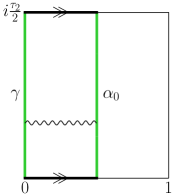
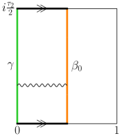
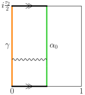
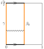
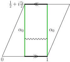
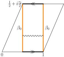
Figure 4: Open-string diagrams of Fig. 3 in the limit $z_{12}\to 0$.

In these expressions, ${\cal C}$ is a constant number, while the supertraces are restricted to the open-string modes with ends attached to branes as shown in Fig. 4. For the identification to be possible, one has to switch the $T^{2}$, $T^{4}$ and $\tilde{T}^{4}$ lattices in the partition functions $Z_{\cal A}$ and $Z_{\cal M}$ from Hamiltonian to instantonic forms, which is done by Poisson summations,

$$\sum_{\vec{m}}P^{(4)}_{\vec{m}+\vec{a}_{i}-\vec{a}_{j}} ={{\rm v}_{4}\over\alpha^{\prime 2}\,\tau_{2}^{2}}\sum_{\vec{l}}e^{-{\pi\over\alpha^{\prime}\tau_{2}}\sum_{I}(R_{I}l_{I})^{2}}e^{2i\pi\vec{l}\cdot(\vec{a}_{i}-\vec{a}_{j})}\,,$$ (5.108)

$$\sum_{\vec{m}}W^{(4)}_{\vec{n}+\vec{a}_{i}-\vec{a}_{j}} ={\alpha^{\prime 2}\over{\rm v}_{4}\,\tau_{2}^{2}}\sum_{\vec{\tilde{l}}}e^{-{\pi\alpha^{\prime}\over\tau_{2}}\sum_{I}({\tilde{l}}_{I}/R_{I})^{2}}e^{2i\pi\vec{\tilde{l}}\cdot(\vec{a}_{i}-\vec{a}_{j})}\,,$$

$$\sum_{\vec{m}^{\prime}}P^{(2)}_{\vec{m}^{\prime}+F\vec{a}_{\rm S}^{\prime}+\vec{a}_{i^{\prime}}-\vec{a}_{j^{\prime}}} ={{\rm v}_{2}\over\alpha^{\prime}\,\tau_{2}}\sum_{\vec{l}^{\prime}}e^{-{\pi\over\alpha^{\prime}\tau_{2}}\sum_{I}(R_{I^{\prime}}l_{I^{\prime}})^{2}}e^{2i\pi\vec{l}^{\prime}\cdot(\vec{a}_{i^{\prime}}-\vec{a}_{j^{\prime}})}e^{2i\pi F\vec{l}^{\prime}\cdot\vec{a}_{\rm S}^{\prime}}\,,$$

where we have defined

$${\rm v}_{4}=R_{6}R_{7}R_{8}R_{9}\,,\leavevmode\nobreak\ \leavevmode\nobreak\ \quad{\rm v}_{2}=R_{4}R_{5}\,.$$ (5.109)

For the case of the annulus, using the definitions of the characters given in Eq. (B.206), we identify

$${\cal C}_{1}^{{\cal A}\vec{l}^{\prime}\vec{l}}=\rho\,{{\cal C}\over\tau_{2}^{2}\,\eta^{3}}\,f_{\alpha_{0}\text{D}}^{{\cal A}\vec{l}^{\prime}\vec{l}}\,, \qquad\tilde{{\cal C}}_{1}^{{\cal A}\vec{l}^{\prime}\vec{\tilde{l}}}=\rho\,{{\cal C}\over\tau_{2}^{2}\,\eta^{3}}\,f_{\beta_{0}\text{N}}^{{\cal A}\vec{l}^{\prime}\vec{\tilde{l}}}\,,$$

$${\cal C}_{2}^{{\cal A}\vec{l}^{\prime}\vec{l}}={{\cal C}\over\tau_{2}^{2}\,\eta^{3}}\,{\vartheta_{3}^{2}\over\vartheta_{4}^{2}}\,f_{\alpha_{0}\text{D}}^{{\cal A}\vec{l}^{\prime}\vec{l}}-{{\cal C}\,\vartheta_{2}^{2}\over\tau_{2}^{4}\,\eta^{9}}\,f_{\alpha_{0}\text{N}}^{{\cal A}\vec{l}^{\prime}\vec{l}}\,e^{2i\pi\vec{l}^{\prime}\cdot\vec{a}_{\rm S}^{\prime}}\,, \qquad\tilde{{\cal C}}_{2}^{{\cal A}\vec{l}^{\prime}\vec{\tilde{l}}}={{\cal C}\over\tau_{2}^{2}\,\eta^{3}}\,{\vartheta_{3}^{2}\over\vartheta_{4}^{2}}\,f_{\beta_{0}\text{N}}^{{\cal A}\vec{l}^{\prime}\vec{\tilde{l}}}-{{\cal C}\,\vartheta_{2}^{2}\over\tau_{2}^{4}\,\eta^{9}}\,f_{\beta_{0}\text{D}}^{{\cal A}\vec{l}^{\prime}\vec{\tilde{l}}}\,e^{2i\pi\vec{l}^{\prime}\cdot\vec{a}_{\rm S}^{\prime}}\,,$$

$${\cal C}_{3}^{{\cal A}\vec{l}^{\prime}\vec{l}}={{\cal C}\,\vartheta_{3}^{2}\over\tau_{2}^{4}\,\eta^{9}}\,f_{\alpha_{0}\text{N}}^{{\cal A}\vec{l}^{\prime}\vec{l}}-{{\cal C}\over\tau_{2}^{2}\,\eta^{3}}\,{\vartheta_{2}^{2}\over\vartheta_{4}^{2}}\,f_{\alpha_{0}\text{D}}^{{\cal A}\vec{l}^{\prime}\vec{l}}\,e^{2i\pi\vec{l}^{\prime}\cdot\vec{a}_{\rm S}^{\prime}}\,, \qquad\tilde{{\cal C}}_{3}^{{\cal A}\vec{l}^{\prime}\vec{\tilde{l}}}={{\cal C}\,\vartheta_{3}^{2}\over\tau_{2}^{4}\,\eta^{9}}\,f_{\beta_{0}\text{D}}^{{\cal A}\vec{l}^{\prime}\vec{\tilde{l}}}-{{\cal C}\over\tau_{2}^{2}\,\eta^{3}}\,{\vartheta_{2}^{2}\over\vartheta_{4}^{2}}\,f_{\beta_{0}\text{N}}^{{\cal A}\vec{l}^{\prime}\vec{\tilde{l}}}\,e^{2i\pi\vec{l}^{\prime}\cdot\vec{a}_{\rm S}^{\prime}}\,,$$

$${\cal C}_{4}^{{\cal A}\vec{l}^{\prime}\vec{l}}=-{{\cal C}\,\vartheta_{4}^{2}\over\tau_{2}^{4}\,\eta^{9}}\,f_{\alpha_{0}\text{N}}^{{\cal A}\vec{l}^{\prime}\vec{l}}\,, \qquad\tilde{{\cal C}}_{4}^{{\cal A}\vec{l}^{\prime}\vec{\tilde{l}}}=-{{\cal C}\,\vartheta_{4}^{2}\over\tau_{2}^{4}\,\eta^{9}}\,f_{\beta_{0}\text{D}}^{{\cal A}\vec{l}^{\prime}\vec{\tilde{l}}}\,,$$ (5.110)

where we have defined

$$f_{\alpha_{0}\text{N}}^{{\cal A}\vec{l}^{\prime}\vec{l}}={{\rm v}_{2}{\rm v}_{4}\over\alpha^{\prime 3}}\,\sum_{i,i^{\prime}}N_{ii^{\prime}}\,e^{2i\pi\vec{l}\cdot(\vec{a}_{i_{0}}-\vec{a}_{i})}e^{2i\pi\vec{l}^{\prime}\cdot(\vec{a}_{i^{\prime}_{0}}-\vec{a}_{i^{\prime}})}\,, f_{\beta_{0}\text{\text{D}}}^{{\cal A}\vec{l}^{\prime}\vec{\tilde{l}}}={{\rm v}_{2}\,\alpha^{\prime 2}\over\alpha^{\prime}\,{\rm v}_{4}}\,\sum_{i,i^{\prime}}D_{ii^{\prime}}\,e^{2i\pi\vec{\tilde{l}}\cdot(\vec{a}_{j_{0}}-\vec{a}_{i})}e^{2i\pi\vec{l}^{\prime}\cdot(\vec{a}_{i^{\prime}_{0}}-\vec{a}_{i^{\prime}})}\,,$$

$$f_{\alpha_{0}\text{D}}^{{\cal A}\vec{l}^{\prime}\vec{l}}=\delta_{\vec{l},\vec{0}}\,{{\rm v}_{2}\over\alpha^{\prime}}\,\sum_{i,i^{\prime}}D_{ii^{\prime}}\,e^{2i\pi\vec{l}^{\prime}\cdot(\vec{a}_{i_{0}^{\prime}}-\vec{a}_{i^{\prime}})}\,, f_{\beta_{0}\text{N}}^{{\cal A}\vec{l}^{\prime}\vec{\tilde{l}}}=\delta_{\vec{\tilde{l}},\vec{0}}\,{{\rm v}_{2}\over\alpha^{\prime}}\,\sum_{i,i^{\prime}}N_{ii^{\prime}}\,e^{2i\pi\vec{l}^{\prime}\cdot(\vec{a}_{i_{0}^{\prime}}-\vec{a}_{i^{\prime}})}\,.$$ (5.111)

To better understand how the discrete sums and coefficients $N_{ii^{\prime}}$ and $D_{ii^{\prime}}$ arise, let us display as an example what the first product of traces in Eq. (2.2) becomes, when restricting to open strings attached (in the T-dual picture) to the D3-brane $\alpha_{0}$, and to a D3-brane $\gamma$ in the Neumann sector,

$$\sum_{\begin{subarray}{c}i,i^{\prime}\\ j,j^{\prime}\end{subarray}}\textrm{tr}(\gamma_{{\rm N},1}^{ii^{\prime}})\textrm{tr}(\gamma_{{\rm N},1}^{jj^{\prime}\,-1})\quad\longrightarrow\quad(\gamma_{{\rm N},1}^{i_{0}i_{0}^{\prime}})_{\alpha_{0}\alpha_{0}}\sum_{j,j^{\prime}}\sum_{\gamma=1}^{N_{jj^{\prime}}}(\gamma_{{\rm N},1}^{jj^{\prime}\,-1})_{\gamma\gamma}=\sum_{j,j^{\prime}}N_{jj^{\prime}}\,.$$ (5.112)

On the contrary, all terms associated with the group generator $g$ vanish, due to the fact that the diagonal components of the matrices $J_{k}$ are zero. In the expressions of ${\cal C}_{1}^{{\cal A}\vec{l}^{\prime}\vec{l}}$ and $\tilde{\cal C}_{1}^{{\cal A}\vec{l}^{\prime}\vec{\tilde{l}}}$, we have introduced a coefficient $\rho$ that accounts for the ambiguity arising in their determination, since $\vartheta_{\nu_{\rm int}}^{2}=0$ for $\nu_{\rm int}=1$. This coefficient will be determined in the sequel. Finally, notice that the identification has lifted all sign ambiguities associated with the twist- and spin-field correlators. These signs depend on the instanton numbers $\vec{l}^{\prime}$, $\vec{l}$, $\vec{\tilde{l}}$ and the positions of the D3-branes $\alpha_{0}$, $\beta_{0}$, $\gamma$.

To perform the similar computation in the Möbius strip case, note that $Z_{\cal M}$ is expressed in terms of “hatted characters” defined in Eq. (2.20). However, in light-cone gauge, the characters associated with the worldsheet fermions multiplied by $1/\hat{\eta}^{8}$ arising from the bosonic coordinates yield low-lying states at the massless level. Hence, all phases $e^{-i\pi(h-c/24)}$ appearing in the definitions of the hatted characters cancel each other and we may simply remove all “hats” on the $\vartheta$ and $\eta$ functions when identifying Eq. (5.107) with the amplitude (5.106). In that case, the normalization functions are found to be

$${\cal C}_{1}^{{\cal M}\vec{l}^{\prime}\vec{l}}=0\,,\qquad {\tilde{{\cal C}}}_{1}^{{\cal M}\vec{l}^{\prime}\vec{\tilde{l}}}=0\,,$$ (5.113)

$${\cal C}_{2}^{{\cal M}\vec{l}^{\prime}\vec{l}}={{\cal C}\,\vartheta_{2}^{2}\over\tau_{2}^{4}\,\eta^{9}}\,{{\rm v}_{2}{\rm v}_{4}\over\alpha^{\prime 3}}\,e^{2i\pi\vec{l}^{\prime}\cdot\vec{a}_{\rm S}^{\prime}}\,,\qquad {\tilde{{\cal C}}}_{2}^{{\cal M}\vec{l}^{\prime}\vec{\tilde{l}}}={{\cal C}\,\vartheta_{2}^{2}\over\tau_{2}^{4}\,\eta^{9}}\,{{\rm v}_{2}\,\alpha^{\prime 2}\over\alpha^{\prime}\,{\rm v}_{4}}\,e^{2i\pi\vec{l}^{\prime}\cdot\vec{a}_{\rm S}^{\prime}}\,,$$

$${\cal C}_{3}^{{\cal M}\vec{l}^{\prime}\vec{l}}=-{{\cal C}\,\vartheta_{3}^{2}\over\tau_{2}^{4}\,\eta^{9}}\,{{\rm v}_{2}{\rm v}_{4}\over\alpha^{\prime 3}}\,,\qquad {\tilde{{\cal C}}}_{3}^{{\cal M}\vec{l}^{\prime}\vec{\tilde{l}}}=-{{\cal C}\,\vartheta_{3}^{2}\over\tau_{2}^{4}\,\eta^{9}}\,{{\rm v}_{2}\,\alpha^{\prime 2}\over\alpha^{\prime}\,{\rm v}_{4}}\,,$$

$${\cal C}_{4}^{{\cal M}\vec{l}^{\prime}\vec{l}}={{\cal C}\,\vartheta_{4}^{2}\over\tau_{2}^{4}\,\eta^{9}}\,{{\rm v}_{2}{\rm v}_{4}\over\alpha^{\prime 3}}\,,\qquad {\tilde{{\cal C}}}_{4}^{{\cal M}\vec{l}^{\prime}\vec{\tilde{l}}}={{\cal C}\,\vartheta_{4}^{2}\over\tau_{2}^{4}\,\eta^{9}}\,{{\rm v}_{2}\,\alpha^{\prime 2}\over\alpha^{\prime}\,{\rm v}_{4}}\,.$$

For instance, when one restricts to the boundary conditions shown in Fig. 4, the first trace appearing in the expression of $Z_{\cal M}$ yields,

$$\textrm{tr}(\gamma_{{\rm N},\Omega}^{ii^{\prime}\,\rm T}\gamma_{{\rm N},\Omega}^{jj^{\prime}\,-1})\quad\longrightarrow\quad(\gamma_{{\rm N},\Omega}^{i_{0}i_{0}^{\prime}\,\rm T})_{\alpha_{0}\alpha_{0}}(\gamma_{{\rm N},\Omega}^{jj^{\prime}\,-1})_{\alpha_{0}\alpha_{0}}=1\,.$$ (5.114)

On the contrary, all traces in the second line of Eq. (2.21) yield vanishing contributions since the selected diagonal matrix elements are zero.

Consistency when supersymmetry is restored:

All normalization functions can be injected back in Eqs. (5.100) and (5.103) to obtain the full expressions of the amplitudes $A_{\rm ext\Sigma}^{\alpha_{0}\beta_{0}}$ and $A_{\rm int\Sigma}^{\alpha_{0}\beta_{0}}$ for arbitrary $z_{1}$, $z_{2}$. To analyze their structures in more details, let us focus on the instantonic sums. For the internal part of the amplitude computed on the annulus, we obtain for each given $\vec{l}^{\prime}$, $\vec{l}$ a contribution of the form

$$\sum_{\nu_{\rm int}}\vartheta_{\nu_{\rm int}}\big{(}{z_{12}\over 2}\big{)}^{2}\,{\cal C}_{\nu_{\rm int}}^{{\cal A}\vec{l}^{\prime}\vec{l}} ={\cal C}\,{f_{\alpha_{0}\rm N}^{{\cal A}\vec{l}^{\prime}\vec{l}}\over\tau_{2}^{4}\,\eta^{9}}\,\bigg{\{}\vartheta_{3}^{2}\vartheta_{3}\big{(}{z_{12}\over 2}\big{)}^{2}-\vartheta_{4}^{2}\vartheta_{4}\big{(}{z_{12}\over 2}\big{)}^{2}-e^{2i\pi\vec{l}^{\prime}\cdot\vec{a}_{\rm S}^{\prime}}\,\vartheta_{2}^{2}\vartheta_{2}\big{(}{z_{12}\over 2}\big{)}^{2}\bigg{\}}$$

$$\;\;\;\;+{\cal C}\,{f_{\alpha_{0}\rm D}^{{\cal A}\vec{l}^{\prime}\vec{l}}\over\tau_{2}^{2}\,\eta^{3}\,\vartheta_{4}^{2}}\,\bigg{\{}\vartheta_{3}^{2}\vartheta_{2}\big{(}{z_{12}\over 2}\big{)}^{2}+\rho\,\vartheta_{4}^{2}\vartheta_{1}\big{(}{z_{12}\over 2}\big{)}^{2}-e^{2i\pi\vec{l}^{\prime}\cdot\vec{a}_{\rm S}^{\prime}}\,\vartheta_{2}^{2}\vartheta_{3}\big{(}{z_{12}\over 2}\big{)}^{2}\bigg{\}}$$

$$={\cal C}\,\big{(}1-(-1)^{l_{5}}\big{)}\bigg{\{}{f_{\alpha_{0}\rm N}^{{\cal A}\vec{l}^{\prime}\vec{l}}\over\tau_{2}^{4}\,\eta^{9}}\,\vartheta_{2}^{2}\vartheta_{2}\big{(}{z_{12}\over 2}\big{)}^{2}+{f_{\alpha_{0}\rm D}^{{\cal A}\vec{l}^{\prime}\vec{l}}\over\tau_{2}^{2}\,\eta^{3}\,\vartheta_{4}^{2}}\,\vartheta_{2}^{2}\vartheta_{3}\big{(}{z_{12}\over 2}\big{)}^{2}\bigg{\}}$$ (5.115)

$$\;\;\;\;+{\cal C}\,(\rho-1)\,{f_{\alpha_{0}\rm D}^{{\cal A}\vec{l}^{\prime}\vec{l}}\over\tau_{2}^{2}\,\eta^{3}}\,\vartheta_{1}\big{(}{z_{12}\over 2}\big{)}^{2}\,,$$

where the second equality is obtained by applying a generalized Jacobi identities [62] with non-zero first arguments, as well as the specific form of the vector $\vec{a}_{\rm S}^{\prime}$. For given $\vec{l}^{\prime}$, $\vec{\tilde{l}}$, the similar sum for the coefficients $\tilde{\cal C}_{\nu_{\rm int}}^{{\cal A}\vec{l}^{\prime}\vec{\tilde{l}}}$ is obtained by changing $\alpha_{0}\to\beta_{0}$ and ${\rm N}\leftrightarrow{\rm D}$. We are now ready to determine the constant $\rho$ by taking the limit $R_{5}\to+\infty$ in Eq. (5.103). Indeed, $l_{5}=0$ is the only contribution in the sum over $l_{5}$ that survives in this limit. Hence, $A_{\text{int}{\cal A}}^{\alpha_{0}\beta_{0}}$ vanishes when supersymmetry is restored if and only if $\rho=1$, since in that case only, Eq. (5.115) projects out all even values of the wrapping number $l_{5}$. Indeed, in the supersymmetric case, the effective potential cannot be corrected perturbatively, which implies $\rho$ to be such that the one-loop corrections to the masses we are computing vanish.

We can proceed the same way for the internal part of the amplitude computed on the Möbius strip. For fixed $\vec{l}^{\prime}$, $\vec{l}$, we have

$$\sum_{\nu_{\rm int}}\vartheta_{\nu_{\rm int}}\big{(}{z_{12}\over 2}\big{)}^{2}\,{\cal C}_{\nu_{\rm int}}^{{\cal M}\vec{l}^{\prime}\vec{l}} ={{\cal C}\,{\rm v}_{2}{\rm v}_{4}\over\alpha^{\prime 3}\,\tau_{2}^{4}\,\eta^{9}}\,\bigg{\{}e^{2i\pi\vec{l}^{\prime}\cdot\vec{a}_{\rm S}^{\prime}}\,\vartheta_{2}^{2}\vartheta_{2}\big{(}{z_{12}\over 2}\big{)}^{2}-\vartheta_{3}^{2}\vartheta_{3}\big{(}{z_{12}\over 2}\big{)}^{2}+\vartheta_{4}^{2}\vartheta_{4}\big{(}{z_{12}\over 2}\big{)}^{2}\bigg{\}}$$ (5.116)

$$=-{{\cal C}\,{\rm v}_{2}{\rm v}_{4}\over\alpha^{\prime 3}\,\tau_{2}^{4}\,\eta^{9}}\,\big{(}1-(-1)^{l_{5}}\big{)}\,\vartheta_{2}^{2}\vartheta_{2}\big{(}{z_{12}\over 2}\big{)}^{2}\,,$$

while for given $\vec{l}^{\prime}$, $\vec{\tilde{l}}$, the analogous sum for $\tilde{\cal C}_{\nu_{\rm int}}^{{\cal M}\vec{l}^{\prime}\vec{l}}$ is obtained by changing ${\rm v}_{4}/\alpha^{\prime 2}\to\alpha^{\prime 2}/{\rm v}_{4}$. In the limit $R_{5}\to+\infty$ where supersymmetry is restored, the amplitude $A_{\text{int}{\cal M}}^{\alpha_{0}\beta_{0}}$ vanishes consistently.

As can be seen from Eqs. (5.100) and (5.103), the sums over the spin structure $\nu_{\rm int}$ in the external and internal parts of the amplitudes are identical, up to the insertion of the sign $(-1)^{\delta_{\nu_{\rm int},1}}$ for $A_{\text{ext}\Sigma}^{\alpha_{0}\beta_{0}}$. Of course, this does not make any difference in the case of the Möbius strip since the normalization functions for $\nu_{\rm int}=1$ vanish. On the contrary, for $\Sigma={\cal A}$, the extra sign amounts to changing $\rho\to-\rho$ in Eq. (5.115). As a result, the external part of the amplitude, $A_{\text{ext}{\cal A}}^{\alpha_{0}\beta_{0}}$, does not vanish in the decompactification limit, and yields a one-loop correction to the Kähler potential of the massless scalars in the ND+DN sector, even in the supersymmetric case.

Integration over the moduli and vertex positions:

What remains to be done is to integrate the amplitudes over the moduli of the open-string surfaces and vertex operator positions modulo the conformal Killing group [63]. The moduli of ${\cal A}$ and ${\cal M}$ are the imaginary parts of the Teichmüller parameters of the double-cover tori, ${\rm Im}\,\tau^{\rm dc}$. Moreover, instead of integrating over the locations of both insertion points and dividing by the volume of the conformal Killing group, we may simply fix to an arbitrary value the position of one vertex operator, say $z_{2}\equiv\frac{1}{2}$, and integrate over the location of the other.

In the case of the annulus, both vertices must be located on the same boundary, so that $z_{1}\equiv\frac{1}{2}+iy_{1}$. As a result, denoting the integrated amplitudes by calligraphic letters, the internal part reads

$$\mathcal{A}_{{\rm int}{\cal A}}^{\alpha_{0}\beta_{0}}=\int_{0}^{+\infty}\text{d}\;\,\!\!{\rm Im}\,\tau^{\rm dc}\int_{0}^{{\rm Im}\,\tau^{\rm dc}}\!\!\!\text{d}y_{1}\left.A_{{\rm int}{\cal A}}^{\alpha_{0}\beta_{0}}\right|_{\frac{1}{2}+iy_{1},\frac{1}{2}},$$ (5.117)

and likewise for the external amplitude. Similarly, for the two-point function computed on the Möbius strip, $z_{1}$ must follow the entire boundary. However, the latter being twice longer than the one considered on the annulus, $z_{1}$ can actually be parametrized as $z_{1}=x_{1}+iy_{1}$, where $x_{1}\in\{0,\frac{1}{2}\}$. As a result, the internal part of the integrated amplitude is

$$\mathcal{A}_{{\rm int}{\cal M}}^{\alpha_{0}\beta_{0}}=\int_{0}^{+\infty}\text{d}\;\,\!\!{\rm Im}\,\tau^{\rm dc}\int_{0}^{{\rm Im}\,\tau^{\rm dc}}\!\!\!\text{d}y_{1}\,\big{(}\!\!\left.A_{{\rm int}{\cal M}}^{\alpha_{0}\beta_{0}}\right|_{\frac{1}{2}+iy_{1},\frac{1}{2}}+\left.A_{{\rm int}{\cal M}}^{\alpha_{0}\beta_{0}}\right|_{iy_{1},\frac{1}{2}}\big{)}\,,$$ (5.118)

and similarly for the external part.

In these forms, the full two-point functions are not particularly illuminating, while performing explicitly the integrals is certainly a hard task. Hence, our goal in the next section is to extract simpler answers valid in the case where the scale of supersymmetry breaking is low.

6 Limit of low supersymmetry breaking scale

The analysis of Ref. [32] is valid in regions of moduli space where the supersymmetry breaking scale $M_{3/2}$ is lower than all other non-vanishing scales present in the model. The reason of this restriction is that extrema of the one-loop effective potential are then easily found, and correspond in the open-string sector to distributing all D3-branes (in the T-dual pictures) on O3-planes. In such a case, the squared masses acquired at one loop by the moduli fields arising from the NN and DD sectors take particularly simple forms, up to exponentially suppressed corrections of order $e^{-\pi\frac{cM_{\rm s}}{M_{3/2}}}$, in the notations of Eq. (1.1). In practice, the fact that $M_{3/2}$ is lower than the string scale as well as all other scales generated by compactification means that, effectively, the dominant contributions of the effective potential and masses derived in Ref. [32] match those found in a Kaluza–Klein field theory in $4+1$ dimensions.

In the present section, we would like to find similar results for the masses of the moduli fields present in the ND+DN sector of the theory. This will be done by imposing all mass scales other than $M_{3/2}$ to be proportional to $M_{\rm s}=1/\sqrt{\alpha^{\prime}}$ and then taking the small $\alpha^{\prime}$ limit.

6.1 Limit of super heavy oscillator states

In order to treat all massive string-oscillator states as super heavy in the Hamiltonian forms of the partition functions, let us rescale the Teichmüller parameters of the open-string surfaces as follows

$${\rm Im}\,\tau^{\rm dc}\equiv{\tau_{2}\over 2}\equiv{t\over 2\pi\alpha^{\prime}}\gg 1\,,\quad\mbox{where}\quad t\in(0,+\infty)\,.$$ (6.119)

Physically, this amounts to stretching the surfaces along their proper times in order to look like field-theory worldlines with topology of a circle. The main practical consequence of the rescaling is the approximation

$$\vartheta_{1}(z) \equiv-2\,q_{\rm dc}^{1\over 8}\sin(\pi z)\prod_{n\geq 1}\big{[}(1-q_{\rm dc}^{n})(1-q_{\rm dc}^{n}z^{-2i\pi z})(1-q_{\rm dc}^{n}z^{2i\pi z})\big{]}\,,\quad q_{\rm dc}\equiv e^{2i\pi\tau^{\rm dc}}\,,$$ (6.120)

$$=-2\,q_{\rm dc}^{1\over 8}\sin(\pi z)(1+\cdots)\,,\quad\mbox{when}\quad|{\rm Im}\,z|<{\rm Im}\,\tau^{\rm dc}\,,$$

where from now on, ellipses stand for terms exponentially suppressed when $\alpha^{\prime}\to 0$, i.e. of order $e^{-L^{2}/\alpha^{\prime}}$ for lengths $L>0$. In particular, the cut differential associated with the complex directions $u\in\{3,4\}$ becomes

$$\omega(z)={\sin\big{(}\pi(z-{z_{1}+z_{2}\over 2})\big{)}\over\sin\!\big{(}\pi(z-z_{1})\big{)}^{\frac{1}{2}}\,\sin\!\big{(}\pi(z-z_{2})\big{)}^{\frac{1}{2}}}+\cdots\,,\quad\mbox{when}\quad|{\rm Im}\,z|,\,y_{1},\,y_{2}<{\rm Im}\,\tau^{\rm dc}\,.$$ (6.121)

Periodicity $z\to z+1$ remains explicit, while periodicity $z\to z+\tau^{\rm dc}$ is hidden in the ellipsis. Notice that compared to Eq. (5.93), we impose $y_{1}$, $y_{2}$ to be strictly lower than ${\rm Im}\,\tau^{\rm dc}$ for the above formula to always be valid. More generally, throughout the derivations to come, we will write formulas in their generic forms. Indeed, because in the end all quantities will have to be integrated, taking into account extra contributions arising only at special values of the integration variables results in subdominant corrections for small $\alpha^{\prime}$. We will come back to this issue at the end of this section.

Keeping this in mind, we redefine

$$y_{A}\equiv u_{A}\,{\rm Im}\,\tau^{\rm dc}={t\,u_{A}\over 2\pi\alpha^{\prime}}\gg 1\,,\quad u_{A}\in(0,1)\,,\leavevmode\nobreak\ \leavevmode\nobreak\ A\in\{1,2\}\,,\leavevmode\nobreak\ \leavevmode\nobreak\ \quad\mbox{and}\leavevmode\nobreak\ \leavevmode\nobreak\ \quad u\equiv|u_{1}-u_{2}|\,,$$ (6.122)

in terms of which the components of the cut-period matrix can be expressed like

$$W_{1} =1+\cdots\,,$$ (6.123)

$$W_{2} =\tau^{\rm dc}-\xi(z_{1}-z_{2})+{i\over\pi}\ln 4+\cdots\,,\quad\mbox{where}\quad\xi\equiv{\rm sign}\,(y_{1}-y_{2})\,.$$

The first expression is easily found by integrating over $z$ finite along $\gamma_{1}$ and replacing all sines in Eq. (6.121) by their dominant exponentials when ${\rm Im}\,\tau^{\rm dc}$ is large. By contrast, $W_{2}$ can be derived by integrating $z$ between $x_{0}$ and $x_{0}+\tau^{\rm dc}$, $x_{0}\in\mathbb{R}$, using a primitive of $\omega$ in its form given in Eq. (6.121). As a result, we obtain that

$${\rm Im}\,(\mkern 1.5mu\overline{\mkern-1.5muW\mkern-1.5mu}\mkern 1.5mu_{1}W_{2})={t(1-u)\over 2\pi\alpha^{\prime}}+{\ln 4\over\pi}+\cdots\,.$$ (6.124)

When taking the limit of small $\alpha^{\prime}$ in Eq. (5.115), it turns out that the terms proportional to $f_{\alpha_{0}\rm D}^{{\cal A}\vec{l}^{\prime}\vec{l}}$ (and $f_{\beta_{0}\rm N}^{{\cal A}\vec{l}^{\prime}\vec{\tilde{l}}}$ for the formula involving $\tilde{\cal C}^{{\cal A}\vec{l}^{\prime}\vec{\tilde{l}}}_{\nu_{\rm int}}$) are exponentially suppressed. Notice that they arise from the ND and DN sectors of the partition function $Z_{\cal A}$, which therefore cease to contribute to the amplitudes in this limit. In the case of the annulus, we then arrive at the expression

$$A_{{\rm int}{\cal A}}^{\alpha_{0}\beta_{0}}= -4{\cal C}s\,\lambda_{\alpha_{0}\beta_{0}}\lambda^{\rm T}_{\beta_{0}\alpha_{0}}\,\sum_{\vec{l}^{\prime}}e^{-{\pi^{2}\over t}\sum_{I^{\prime}}(R_{I^{\prime}}l_{I^{\prime}})^{2}}\,\sum_{\vec{l}}e^{-{\pi^{2}\over t(1-u)+\alpha^{\prime}(2\ln 4+\cdots\mbox{\tiny$\!\,$})}\sum_{I}(R_{I}l_{I})^{2}}\,\times$$

$$\,\big{(}1-(-1)^{l_{5}}\big{)}\,2\pi^{3}\,{\alpha^{\prime 4}\over t^{4}}\,{{\rm v}_{2}{\rm v}_{4}\over\alpha^{\prime 3}}\,\sum_{ii^{\prime}}N_{ii^{\prime}}\,e^{2i\pi\vec{l}\cdot(\vec{a}_{i_{0}}-\vec{a}_{i})}e^{2i\pi\vec{l}^{\prime}\cdot(\vec{a}_{i^{\prime}_{0}}-\vec{a}_{i^{\prime}})}\,\times$$ (6.125)

$$\,{\pi\over t(1-u)+\alpha^{\prime}(2\ln 4+\cdots)}\,\bigg{[}{\pi^{4}\,\alpha^{\prime 2}\over[t(1-u)+\alpha^{\prime}(2\ln 4+\cdots)]^{2}}\sum_{J}(R_{J}l_{J})^{2}+2\alpha^{\prime}(C+\hat{C})\bigg{]}$$

$$+(\vec{l},i_{0},N_{ii^{\prime}},R_{I})\to(\vec{\tilde{l}},j_{0},D_{ii^{\prime}},\alpha^{\prime}/R_{I})+\cdots\,,\phantom{\!\!\!\overset{|}{a}}$$

while for the Möbius strip we obtain

$$A_{{\rm int}{\cal M}}^{\alpha_{0}\beta_{0}}= \;4{\cal C}s\,\lambda_{\alpha_{0}\beta_{0}}\lambda^{\rm T}_{\beta_{0}\alpha_{0}}\,\sum_{\vec{l}^{\prime}}e^{-{\pi^{2}\over t}\sum_{I^{\prime}}(R_{I^{\prime}}l_{I^{\prime}})^{2}}\,\sum_{\vec{l}}e^{-{\pi^{2}\over t(1-u)+\alpha^{\prime}(2\ln 4+\cdots\mbox{\tiny$\!\,$})}\sum_{I}(R_{I}l_{I})^{2}}\,\times$$

$$\,\big{(}1-(-1)^{l_{5}}\big{)}\,2\pi^{3}\,{\alpha^{\prime 4}\over t^{4}}\,{{\rm v}_{2}{\rm v}_{4}\over\alpha^{\prime 3}}\,\times$$ (6.126)

$$\,{\pi\over t(1-u)+\alpha^{\prime}(2\ln 4+\cdots)}\,\bigg{[}{\pi^{4}\,\alpha^{\prime 2}\over[t(1-u)+\alpha^{\prime}(2\ln 4+\cdots)]^{2}}\sum_{J}(R_{J}l_{J})^{2}+2\alpha^{\prime}(C+\hat{C})\bigg{]}$$

$$+(\vec{l},R_{I})\to(\vec{\tilde{l}},\alpha^{\prime}/R_{I})+\cdots\,.\phantom{\!\!\!\overset{|}{a}}$$

In the above formulas, the limit of small $\alpha^{\prime}$ in $C$ and $\hat{C}$ will be derived in Sects. 6.3 and 6.4.

6.2 Limits of large compactification scales

We would like now to have all compactification mass scales other than $M_{3/2}$ very large. In practice, this amounts to taking small radii $R_{4}$, $R_{I}$ and dual radii $\alpha^{\prime}/R_{I}$ limits. In order to avoid having to consider very large instanton numbers in such a regime, it is convenient to apply Poisson summations over $l_{4}$, $\vec{l}$ and $\vec{\tilde{l}}$ [62], which lead for $\Sigma={\cal A}$ to

$$A_{{\rm int}{\cal A}}^{\alpha_{0}\beta_{0}}= -16{\cal C}s\sqrt{\pi}\,\lambda_{\alpha_{0}\beta_{0}}\lambda^{\rm T}_{\beta_{0}\alpha_{0}}\,{\alpha^{\prime 3}R_{5}\over t^{7\over 2}}\,\sum_{l_{5}}e^{-{\pi^{2}\over t}R_{5}^{2}(2l_{5}+1)^{2}}\,\sum_{ii^{\prime}}N_{ii^{\prime}}\,e^{2i\pi(a^{5}_{i_{0}^{\prime}}-a^{5}_{i^{\prime}})}$$ (6.127)

$$\times\sum_{m_{4}}e^{-t\big{(}{m_{4}+a^{4}_{i_{0}^{\prime}}-a^{4}_{i^{\prime}}\over R_{4}}\big{)}^{2}}\,\sum_{\vec{m}}e^{-[t(1-u)+\alpha^{\prime}(2\ln 4+\cdots\mbox{\tiny$\!\,$})]\sum_{I}\big{(}{m_{I}+a^{I}_{i_{0}}-a^{I}_{i}\over R_{I}}\big{)}^{2}}$$

$$\times\bigg{\{}\pi^{3}\bigg{[}2-[t(1-u)+\alpha^{\prime}(2\ln 4+\cdots)]\sum_{J}\Big{(}{m_{J}+a^{J}_{i_{0}}-a^{J}_{i}\over R_{J}}\Big{)}^{2}\bigg{]}$$

$$\;\;\;\;\;+2\pi\bigg{[}{t(1-u)\over\alpha^{\prime}}+2\ln 4+\cdots\bigg{]}(C+\hat{C})\bigg{\}}$$

$$\;+(\vec{m},i_{0},N_{ii^{\prime}},R_{I})\to(\vec{n},j_{0},D_{ii^{\prime}},\alpha^{\prime}/R_{I})+\cdots\,,\phantom{\!\!\!\overset{|}{a}}$$

and for $\Sigma={\cal M}$

$$A_{{\rm int}{\cal M}}^{\alpha_{0}\beta_{0}}= \,16{\cal C}s\sqrt{\pi}\,\lambda_{\alpha_{0}\beta_{0}}\lambda^{\rm T}_{\beta_{0}\alpha_{0}}\,{\alpha^{\prime 3}R_{5}\over t^{7\over 2}}\,\sum_{l_{5}}e^{-{\pi^{2}\over t}R_{5}^{2}(2l_{5}+1)^{2}}$$ (6.128)

$$\times\sum_{m_{4}}e^{-t({m_{4}\over R_{4}})^{2}}\,\sum_{\vec{m}}e^{-[t(1-u)+\alpha^{\prime}(2\ln 4+\cdots\mbox{\tiny$\!\,$})]\sum_{I}({m_{I}\over R_{I}})^{2}}$$

$$\times\bigg{\{}\pi^{3}\bigg{[}2-[t(1-u)+\alpha^{\prime}(2\ln 4+\cdots)]\sum_{J}\Big{(}{m_{J}\over R_{J}}\Big{)}^{2}\bigg{]}$$

$$\;\;\;\;\;+2\pi\bigg{[}{t(1-u)\over\alpha^{\prime}}+2\ln 4+\cdots\bigg{]}(C+\hat{C})\bigg{\}}$$

$$\;+(\vec{m},R_{I})\to(\vec{n},\alpha^{\prime}/R_{I})+\cdots\,.\phantom{\!\!\!\overset{|}{a}}$$

One may think that considering $T^{4}$ to be small would imply having the T-dual torus $\tilde{T}^{4}$ large. This is not true, as can be seen by redefining the radii as follows,

$$R_{4}=r_{4}\sqrt{\alpha^{\prime}}\,,\leavevmode\nobreak\ \leavevmode\nobreak\ \quad R_{I}=r_{I}\sqrt{\alpha^{\prime}}\,,\leavevmode\nobreak\ \leavevmode\nobreak\ \quad{\alpha^{\prime}\over R_{I}}={\sqrt{\alpha^{\prime}}\over r_{I}}\,,$$ (6.129)

where $r_{4}$, $r_{I}$ are fixed and dimensionless. Indeed, all radii and dual radii vanish as $\alpha^{\prime}\to 0$. As a consequence, the limit of small $R_{4}$ implies that we may restrict the dominant term in $A_{{\rm int}{\cal A}}^{\alpha_{0}\beta_{0}}$ to $m_{4}=0$ and $i^{\prime}\in\{i_{0}^{\prime},\hat{\imath}_{0}^{\prime}\}$, where

$$\hat{\imath}_{0}^{\prime} \tilde{T}^{2} i_{0}^{\prime} \tilde{X}^{5}$$ is the fixed point in that faces along the direction (6.130)

in the T-dual pictures. Similarly, the limits of small $R_{I}$ and $\alpha^{\prime}/R_{I}$ force $\vec{m}=0$, $i=i_{0}$ on the one hand, and $\vec{n}=0$, $i=j_{0}$ on the other hand. All other contributions can be absorbed in the ellipsis. In total, we obtain for the amplitude computed on the annulus

$$A_{{\rm int}{\cal A}}^{\alpha_{0}\beta_{0}}= -16{\cal C}s\sqrt{\pi}\,\lambda_{\alpha_{0}\beta_{0}}\lambda^{\rm T}_{\beta_{0}\alpha_{0}}\,{\alpha^{\prime 3}R_{5}\over t^{7\over 2}}\,\sum_{l_{5}}e^{-{\pi^{2}\over t}R_{5}^{2}(2l_{5}+1)^{2}}\,\big{(}N_{i_{0}i_{0}^{\prime}}-N_{i_{0}\hat{\imath}_{0}^{\prime}}+D_{j_{0}i_{0}^{\prime}}-D_{j_{0}\hat{\imath}_{0}^{\prime}}\big{)}$$ (6.131)

$$\times\bigg{\{}2\pi^{3}+2\pi\bigg{[}{t(1-u)\over\alpha^{\prime}}+2\ln 4+\cdots\bigg{]}(C+\hat{C})\bigg{\}}+\cdots\,,$$

while on the Möbius strip we have similarly

$$A_{{\rm int}{\cal M}}^{\alpha_{0}\beta_{0}}= \;16{\cal C}s\sqrt{\pi}\,\lambda_{\alpha_{0}\beta_{0}}\lambda^{\rm T}_{\beta_{0}\alpha_{0}}\,{\alpha^{\prime 3}R_{5}\over t^{7\over 2}}\,\sum_{l_{5}}e^{-{\pi^{2}\over t}R_{5}^{2}(2l_{5}+1)^{2}}\,(1+1)$$ (6.132)

$$\times\bigg{\{}2\pi^{3}+2\pi\bigg{[}{t(1-u)\over\alpha^{\prime}}+2\ln 4+\cdots\bigg{]}(C+\hat{C})\bigg{\}}+\cdots\,.$$

6.3 Limit $\alpha^{\prime}\to 0$ of $U_{1}$ and $F_{1}(z,z_{2})$

In this subsection and the following, our aim is to derive the limits of $C$ and $\hat{C}$ for small $\alpha^{\prime}$, i.e. the contributions arising from parts $(2)$ of the correlators $\langle\tau^{u}\tau^{\prime u}\rangle_{\text{qu}}=\langle\tau^{\prime u}\tau^{u}\rangle_{\text{qu}}$. Because the results can be obtained with no more effort for any Teichmüller parameter, we will keep the real part of $\tau^{\rm dc}$ arbitrary, and $z_{1}$, $z_{2}$ will be chosen anywhere in the torus represented by ${\cal P}$ in the complex plane, where

$$\mbox{${\cal P}$ is the parallelogram with corners at 0, 1 and $\tau^{\rm dc}$}\,.$$ (6.133)

The important thing, though, is that Eqs. (6.119) and (6.122) hold. Hence, our computations of parts $(2)$ are valid for excited twist fields (for closed strings) and excited boundary-changing fields (for open strings). Let us start by deriving the limits of $U_{1}$ and $F_{1}(z,z_{2})$, which will be used in the next subsection to derive those of $C$ and $\hat{C}$.

$U_{1}$ when $\alpha^{\prime}\to 0$:

The function $F_{1}(z,w)$ defined in Eq. (4.85) involves $U_{1}$ which is a root of

$$\Omega(U)\equiv\partial_{z}F_{1}(z,w)|_{z=w}={\vartheta_{1}^{\prime}\over\vartheta_{1}}(U)+{\vartheta_{1}^{\prime}\over\vartheta_{1}}(Y_{1}-U)\,,\quad\mbox{where}\quad Y_{1}=-{z_{12}\over 2}\,.$$ (6.134)

To see that this definition makes sense, notice that the meromorphic function $\Omega(U)$ is doubly periodic on the genus-1 Riemann surface $\Sigma$, with two simple poles at $U=0$ and $U=Y_{1}$. Therefore, it has two simple zeros. Denoting one of them $U_{1}$, the second is $Y_{1}-U_{1}$.

When considering the limit $\alpha^{\prime}\to 0$ in the equation $\Omega(U_{1})=0$, a difficulty we have to face is the following: If we look for $U_{1}$ such that $0<{\rm Im}\,U_{1}<{\rm Im}\,\tau^{\rm dc}$, using the fact that $|{\rm Im}\,Y_{1}|<\frac{1}{2}\,{\rm Im}\,\tau^{\rm dc}$ we obtain that

$$-{3\over 2}\,{\rm Im}\,\tau^{\rm dc}<{\rm Im}\,(Y_{1}-U_{1})<\frac{1}{2}\,{\rm Im}\,\tau^{\rm dc}\,.$$ (6.135)

Hence, it is not clear when we can apply Eq. (6.120) or not. For this reason, let us consider two cases:

• When $0<{\rm Im}\,Y_{1}<\frac{1}{2}\,{\rm Im}\,\tau^{\rm dc}$, we obtain that $|{\rm Im}\,(Y_{1}-U_{1})|<\frac{1}{2}\,{\rm Im}\,\tau^{\rm dc}$ which allows to write

  $$0=\Omega(U_{1}) =\pi\big{(}\!\cot(\pi U_{1})+\cot[\pi(Y_{1}-U_{1})]\big{)}+\cdots$$ (6.136)

  $$=\pi\,{\sin(\pi Y_{1})\over\sin(\pi U_{1})\sin[\pi(Y_{1}-U_{1})]}+\cdots\,.$$

  For the right-hand side to vanish when $\alpha^{\prime}\to 0$, we see that $U_{1}$ must satisfy ${\rm Im}\,U_{1}\to+\infty$ and ${\rm Im}\,(Y_{1}-U_{1})<0$. To determine $U_{1}$ more precisely, let us keep the first subdominant term in the ellipsis of Eq. (6.136), which is $2i\pi\,q_{\rm dc}\,e^{-2i\pi U_{1}}$. In that case, the equation becomes

  $$i\sin(\pi Y_{1})=2\sin(\pi U_{1})\sin[\pi(Y_{1}-U_{1})]\,q_{\rm dc}\,e^{-2i\pi U_{1}}(1+\cdots)\,,$$ (6.137)

  which implies the asymptotic equivalence

  $$-e^{-i\pi Y_{1}}\underset{\alpha^{\prime}\to 0}{\sim}e^{-i\pi U_{1}}\,e^{i\pi(Y_{1}-U_{1})}\,q_{\rm dc}\,e^{-2i\pi U_{1}}\,.$$ (6.138)

  Redefining

  $$U_{1}\equiv{\tau^{\rm dc}+Y_{1}\over 2}+{1\over 4}+{m\over 2}+\varepsilon\quad\mbox{for some }m\in\mathbb{Z}\,,\quad\mbox{with}\quad|{\rm Re}\,\varepsilon|<\frac{1}{2}\,,$$ (6.139)

  Eq. (6.138) shows that $\varepsilon\to 0$ when $\alpha^{\prime}\to 0$.

• When $-\frac{1}{2}\,{\rm Im}\,\tau^{\rm dc}<{\rm Im}\,Y_{1}<0$, we can apply the change of variable (6.139) which yields

  $$-{3\over 4}\,{\rm Im}\,\tau^{\rm dc}-{\rm Im}\,\varepsilon<{\rm Im}\,(Y_{1}-U_{1})<-\frac{1}{2}\,{\rm Im}\,\tau^{\rm dc}-{\rm Im}\,\varepsilon\,.$$ (6.140)

  Hence, assuming that $\varepsilon$ is bounded when $\alpha^{\prime}\to 0$, Eq. (6.136) is legitimate for small enough $\alpha^{\prime}$. However, the first dominant term in the ellipsis is now $-2i\pi\,q_{\rm dc}\,e^{2i\pi(Y_{1}-U_{1})}$,${}^{\ref{footn}}$ and the equation becomes

  $$i\sin(\pi Y_{1})=-2\sin(\pi U_{1})\sin[\pi(Y_{1}-U_{1})]\,q_{\rm dc}\,e^{2i\pi(Y_{1}-U_{1})}(1+\cdots)\,.$$ (6.141)

  Hence, we obtain that

  $$e^{i\pi Y_{1}}\underset{\alpha^{\prime}\to 0}{\sim}-e^{-i\pi U_{1}}\,e^{i\pi(Y_{1}-U_{1})}\,q_{\rm dc}\,e^{2i\pi(Y_{1}-U_{1})}\,,$$ (6.142)

  which is equivalent to Eq. (6.138) and leads to $\varepsilon\to 0$ when $\alpha^{\prime}\to 0$. The assumption on the boundedness of $\varepsilon$ being consistent, we have also found solutions in the present case.

In both instances, $\varepsilon$ can be expressed in terms of exponentially suppressed contributions subdominant to those we have taken into account explicitly. Its leading behavior is derived in Appendix C.

By imposing $U_{1}$ to be located in ${\cal P}$, we find the two roots of $\Omega(U)$,

$$U_{1}={\tau^{\rm dc}+Y_{1}\over 2}+{1\over 4}+\cdots\quad\mbox{or}\quad{\tau^{\rm dc}+Y_{1}\over 2}+{3\over 4}+\cdots\,.$$ (6.143)

Since we know that there cannot be other solutions modulo 1 and $\tau^{\rm dc}$, a cross-check of this result is to observe that $Y_{1}-U_{1}$ satisfies consistently

$$Y_{1}-U_{1}+1+\tau^{\rm dc}={\tau^{\rm dc}+Y_{1}\over 2}+{3\over 4}+\cdots\quad\mbox{or}\quad{\tau^{\rm dc}+Y_{1}\over 2}+{1\over 4}+\cdots\,.$$ (6.144)

$F_{1}(z,z_{2})$ when $\alpha^{\prime}\to 0$:

Both possible choices of $U_{1}$ yield the same function $F_{1}(z,w)$. What we need to analyze in order to derive the limits of $C$ and $\hat{C}$ is its expression for $w=z_{2}$,

$$F_{1}(z,z_{2})={\vartheta_{1}\big{(}z+{\tau^{\rm dc}\over 2}-{1\over 4}\,z_{1}-{3\over 4}\,z_{2}+{1\over 4}+\cdots\big{)}\,\vartheta_{1}\big{(}z-{\tau^{\rm dc}\over 2}-{1\over 4}\,z_{1}-{3\over 4}\,z_{2}-{1\over 4}+\cdots\big{)}\over\vartheta_{1}\big{(}{\tau^{\rm dc}\over 2}-{z_{12}\over 4}+{1\over 4}+\cdots\big{)}\,\vartheta_{1}\big{(}-{\tau^{\rm dc}\over 2}-{z_{12}\over 4}-{1\over 4}+\cdots\big{)}}\,,$$ (6.145)

where $z\equiv x+iy\in{\cal P}$, and $x$, $y\in\mathbb{R}$. Notice that Eq. (6.120) can be applied to both $\vartheta_{1}$ functions appearing in the denominator (for small enough $\alpha^{\prime}$).

For $0<{1\over 2}\,y_{1}+{3\over 2}\,y_{2}<{\rm Im}\,\tau^{\rm dc}$, the second $\vartheta_{1}$ function in the numerator fulfils the hypothesis of Eq. (6.120), while the first one requires more scrutiny:

• When $0<y<\frac{1}{2}\,{\rm Im}\,\tau^{\rm dc}+{1\over 4}\,y_{1}+{3\over 4}\,y_{2}$, Eq. (6.120) applies to the first $\vartheta_{1}$.

• When $\frac{1}{2}\,{\rm Im}\,\tau^{\rm dc}+{1\over 4}\,y_{1}+{3\over 4}\,y_{2}<y<{\rm Im}\,\tau^{\rm dc}$, we have (for small enough $\alpha^{\prime}$)

  $${\rm Im}\,\tau^{\rm dc}<{\rm Im}\,\Big{(}z+{\tau^{\rm dc}\over 2}-{1\over 4}\,z_{1}-{3\over 4}\,z_{2}+{1\over 4}+\cdots\Big{)}<{3\over 2}\,{\rm Im}\,\tau^{\rm dc}\,,$$ (6.146)

  which shows that we have to multiply the second line of Eq. (6.120) by an extra factor $-q_{\rm dc}e^{-2i\pi z}$ to apply it to the first $\vartheta_{1}$ function in the numerator of Eq. (6.145).

In the end, we obtain that

$$\mbox{when}\quad 0<\mbox{$\frac{1}{2}$}\,y_{1}+\mbox{${3\over 2}$}\,y_{2}<{\rm Im}\,\tau^{\rm dc}\,,\quad\mbox{then}$$ (6.147)

$$F_{1}(z,z_{2})=\left\{\begin{array}[]{ll}1+\cdots&\mbox{if\leavevmode\nobreak\ \leavevmode\nobreak\ $0<y<\frac{1}{2}\,{\rm Im}\,\tau^{\rm dc}+{1\over 4}\,y_{1}+{3\over 4}\,y_{2}$}\,,\\ e^{-4i\pi(z-{\tau^{\rm dc}\over 2}-{1\over 4}z_{1}-{3\over 4}z_{2})}\,(1+\cdots)&\mbox{if\leavevmode\nobreak\ \leavevmode\nobreak\ $\frac{1}{2}\,{\rm Im}\,\tau^{\rm dc}+{1\over 4}\,y_{1}+{3\over 4}\,y_{2}<y<{\rm Im}\,\tau^{\rm dc}$\,.}\end{array}\right.$$ (6.150)

Conversely, for ${\rm Im}\,\tau^{\rm dc}<\frac{1}{2}\,y_{1}+{3\over 2}\,y_{2}<2\,{\rm Im}\,\tau^{\rm dc}$, it is the first $\vartheta_{1}$ function in the numerator that satisfies the condition of validity of Eq. (6.120), while for the second one we have to consider two possibilities:

• When ${1\over 4}\,y_{1}+{3\over 4}\,y_{2}-\frac{1}{2}\,{\rm Im}\,\tau^{\rm dc}<y<{\rm Im}\,\tau^{\rm dc}$, Eq. (6.120) applies to this $\vartheta_{1}$ function.

• When $0<y<{1\over 4}\,y_{1}+{3\over 4}\,y_{2}-\frac{1}{2}\,{\rm Im}\,\tau^{\rm dc}$, we have (for small enough $\alpha^{\prime}$)

  $$-{3\over 2}\,{\rm Im}\,\tau^{\rm dc}<{\rm Im}\,\Big{(}z-{\tau^{\rm dc}\over 2}-{1\over 4}\,z_{1}-{3\over 4}\,z_{2}-{1\over 4}+\cdots\Big{)}<-{1\over 2}\,{\rm Im}\,\tau^{\rm dc}\,.$$ (6.151)

  Hence, the second line of Eq. (6.120) must contain an extra factor $-q_{\rm dc}e^{2i\pi z}$ to apply it to the second $\vartheta_{1}$ function in the numerator of $F_{1}(z,z_{2})$.

All in all,

$$\mbox{when}\quad{\rm Im}\,\tau^{\rm dc}<\mbox{$\frac{1}{2}$}\,y_{1}+\mbox{${3\over 2}$}\,y_{2}<2\,{\rm Im}\,\tau^{\rm dc}\,,\quad\mbox{then}$$ (6.152)

$$F_{1}(z,z_{2})=\left\{\begin{array}[]{ll}e^{4i\pi(z-{1\over 4}z_{1}-{3\over 4}z_{2}+{\tau^{\rm dc}\over 2})}\,(1+\cdots)&\mbox{if\leavevmode\nobreak\ \leavevmode\nobreak\ $0<y<{1\over 4}\,y_{1}+{3\over 4}\,y_{2}-\frac{1}{2}\,{\rm Im}\,\tau^{\rm dc}$\,,}\\ 1+\cdots&\mbox{if\leavevmode\nobreak\ \leavevmode\nobreak\ ${1\over 4}\,y_{1}+{3\over 4}\,y_{2}-\frac{1}{2}\,{\rm Im}\,\tau^{\rm dc}<y<{\rm Im}\,\tau^{\rm dc}$}\,.\phantom{\!\!\!\overset{|}{a}}\end{array}\right.$$ (6.155)

6.4 Limit $\alpha^{\prime}\to 0$ of $C$ and $\hat{C}$

We are now ready to evaluate the limits of $C$ and $\hat{C}$ for small $\alpha^{\prime}$.

$\hat{C}$ when $\alpha^{\prime}\to 0$:

The expression of $\hat{C}$ given in Eq. (5.104) involves $F_{1}(z_{1},z_{2})$. If this quantity can certainly be obtained by taking $z=z_{1}$ in the results we have just derived, it can also be computed from scratch by reasoning in the same way, which turns out to be easier. The result is

$$F_{1}(z_{1},z_{2})=\left\{\begin{array}[]{llrll}e^{2i\pi(\tau^{\rm dc}-{3\over 2}z_{12})}(1+\cdots)&\mbox{if}\!\!&{2\over 3}\,{\rm Im}\,\tau^{\rm dc}\!\!\!\!&<{\rm Im}\,z_{12}\!\!\!\!&<{\rm Im}\,\tau^{\rm dc}\,,\\ (1+\cdots)&\mbox{if}\!\!&-{2\over 3}\,{\rm Im}\,\tau^{\rm dc}\!\!\!\!&<{\rm Im}\,z_{12}\!\!\!\!&<{2\over 3}\,{\rm Im}\,\tau^{\rm dc}\,,\phantom{\!\!\!\overset{|}{a}}\\ e^{2i\pi(\tau^{\rm dc}+{3\over 2}z_{12})}(1+\cdots)&\mbox{if}\!\!\!&-{\rm Im}\,\tau^{\rm dc}\!\!\!&<{\rm Im}\,z_{12}\!\!\!\!&<-{2\over 3}\,{\rm Im}\,\tau^{\rm dc}\,.\phantom{\!\!\!\overset{|}{a}}\end{array}\right.$$ (6.156)

As a result, the contributions proportional to $\hat{C}$ in Eqs. (6.131) and (6.132) are of the form

$$2\pi\bigg{[}{t(1-u)\over\alpha^{\prime}}+2\ln 4+\cdots\bigg{]}\hat{C} =-4\pi^{3}\bigg{[}{t(1-u)\over\alpha^{\prime}}+2\ln 4+\cdots\bigg{]}\times$$

$$\leavevmode\nobreak\ \leavevmode\nobreak\ \leavevmode\nobreak\ \left\{\begin{array}[]{llrll}e^{2i\pi(\tau^{\rm dc}-z_{12})}(1+\cdots)&\mbox{if}\!\!&{2\over 3}\,{\rm Im}\,\tau^{\rm dc}\!\!\!\!&<{\rm Im}\,z_{12}\!\!\!\!&<{\rm Im}\,\tau^{\rm dc}\,,\\ e^{i\pi z_{12}}(1+\cdots)&\mbox{if}\!\!&0\!\!\!\!&<{\rm Im}\,z_{12}\!\!\!\!&<{2\over 3}\,{\rm Im}\,\tau^{\rm dc}\,,\phantom{\!\!\!\overset{|}{a}}\\ e^{-i\pi z_{12}}(1+\cdots)&\mbox{if}\!\!&-{2\over 3}\,{\rm Im}\,\tau^{\rm dc}\!\!\!\!&<{\rm Im}\,z_{12}\!\!\!\!&<0\,,\phantom{\!\!\!\overset{|}{a}}\\ e^{2i\pi(\tau^{\rm dc}+z_{12})}(1+\cdots)&\mbox{if}\!\!\!&-{\rm Im}\,\tau^{\rm dc}\!\!\!&<{\rm Im}\,z_{12}\!\!\!\!&<-{2\over 3}\,{\rm Im}\,\tau^{\rm dc}\,,\phantom{\!\!\!\overset{|}{a}}\end{array}\right.$$ (6.161)

$$=\cdots\,,$$ (6.162)

which is exponentially suppressed. Note however that this statement is valid when the intervals of ${\rm Im}\,z_{12}$ are open.

$C$ when $\alpha^{\prime}\to 0$:

Using the relation given in Eq. (4.87), the term linear in $C$ in Eqs. (6.131) and (6.132) can be written as

$$2\pi\bigg{[}{t(1-u)\over\alpha^{\prime}}+2\ln 4+\cdots\bigg{]}C=-2i\pi^{4}\cos\!\Big{(}{\pi\over 2}\,z_{12}\Big{)}\big{[}\mkern 1.5mu\overline{\mkern-1.5muW\mkern-1.5mu}\mkern 1.5mu_{2}\,{\cal F}_{1}-{\cal F}_{2}\big{]}\,,$$ (6.163)

where $${\cal F}_{a}=\oint_{\gamma_{a}}\text{d}z\,{F_{1}(z,z_{2})\,(1+\cdots)\over\sin[\pi(z-z_{1})]^{\frac{1}{2}}\sin[\pi(z-z_{2})]^{3\over 2}}\,,\quad a\in\{1,2\}\,,\phantom{\!\!\overset{\displaystyle|}{|}}$$

and $W_{2}$ is given in Eq. (6.123). We are going to show that ${\cal F}_{1}$ contributes exponentially suppressed terms while ${\cal F}_{2}$ yields a finite result.

In order to evaluate ${\cal F}_{1}$, we impose the points $z$ of the representative path of the cycle $\gamma_{1}$ to satisfy ${\rm Im}\,z\equiv\frac{1}{2}\,{\rm Im}\,\tau^{\rm dc}$. The advantage of this choice is that $F_{1}(z,z_{2})$ can be replaced by $1+\cdots$ all along the path,

$${\cal F}_{1}=\int_{0}^{1}\text{d}x\,{1+\cdots\over\sin[\pi(x+{\tau^{\rm dc}\over 2}-z_{1})]^{\frac{1}{2}}\sin[\pi(x+{\tau^{\rm dc}\over 2}-z_{2})]^{3\over 2}}\,.$$ (6.164)

Omitting the ellipsis, an explicit integration using a primitive of the integrand yields an exactly vanishing result. However, the exponentially suppressed terms in the numerator may be large once multiplied by $\cos(\pi z_{12}/2)$. To take them into account, one can find upper bounds valid for given signs of $\frac{1}{2}\,{\rm Im}\,\tau^{\rm dc}-y_{1}$, $\frac{1}{2}\,{\rm Im}\,\tau^{\rm dc}-y_{2}$ and $y_{1}-y_{2}$. As an example, when $(\frac{1}{2}\,{\rm Im}\,\tau^{\rm dc}-y_{1})(\frac{1}{2}\,{\rm Im}\,\tau^{\rm dc}-y_{2})<0$ we obtain

$$\Big{|}\cos\!\Big{(}{\pi\over 2}\,z_{12}\Big{)}\,{\cal F}_{1}\Big{|}\leq\int_{0}^{1}\text{d}x\,4\,e^{-\pi|\frac{1}{2}{\rm Im}\,\tau^{\rm dc}-y_{2}|}\,K=\cdots\,,$$ (6.165)

where the constant $K$ is any majorant of $|1+\cdots|$ for small enough $\alpha^{\prime}$. It turns out that in all instances the contributions proportional to ${\cal F}_{1}$ are suppressed.

To compute ${\cal F}_{2}$, we have to consider two cases. When $0<\mbox{$\frac{1}{2}$}\,y_{1}+\mbox{${3\over 2}$}\,y_{2}<{\rm Im}\,\tau^{\rm dc}$, Eq. (6.147) allows us to decompose the integral into two pieces,

$${\cal F}_{2}={\cal F}_{2}^{(1)}+{\cal F}_{2}^{(2)}\,,$$ (6.166)

where $${\cal F}_{2}^{(1)}=\int_{0}^{{\tau^{\rm dc}\over 2}+{1\over 4}z_{1}+{3\over 4}z_{2}}\text{d}z\,{1+\cdots\over\sin[\pi(z-z_{1})]^{\frac{1}{2}}\sin[\pi(z-z_{2})]^{3\over 2}}\,,$$

$${\cal F}_{2}^{(2)}=\int^{\tau^{\rm dc}}_{{\tau^{\rm dc}\over 2}+{1\over 4}z_{1}+{3\over 4}z_{2}}\text{d}z\,{e^{-4i\pi(z-{\tau^{\rm dc}\over 2}-{1\over 4}z_{1}-{3\over 4}z_{2})}\,(1+\cdots)\over\sin[\pi(z-z_{1})]^{\frac{1}{2}}\sin[\pi(z-z_{2})]^{3\over 2}}\,.$$

A primitive of the leading term of the integrand of ${\cal F}_{2}^{(1)}$ can be found and the limit of small $\alpha^{\prime}$ taken after integration. This second step requires considering two cases, namely

$$(a):\leavevmode\nobreak\ y_{1}-y_{2}<{2\over 3}\,{\rm Im}\,\tau^{\rm dc}\quad\leavevmode\nobreak\ \leavevmode\nobreak\ \mbox{and}\leavevmode\nobreak\ \leavevmode\nobreak\ \quad(b):\leavevmode\nobreak\ y_{1}-y_{2}>{2\over 3}\,{\rm Im}\,\tau^{\rm dc}\,,$$ (6.167)

which turn out to yield identical finite results,

$$\cos\!\Big{(}{\pi\over 2}\,z_{12}\Big{)}\int_{0}^{{\tau^{\rm dc}\over 2}+{1\over 4}z_{1}+{3\over 4}z_{2}}\text{d}z\,{1\over\sin[\pi(z-z_{1})]^{\frac{1}{2}}\sin[\pi(z-z_{2})]^{3\over 2}}={2i\over\pi}+\cdots\,.$$ (6.168)

The extra contribution arising from the ellipsis in the integrand of ${\cal F}_{2}^{(1)}$ turns out to be exponentially suppressed. However, this is not totally obvious since the dominant implicit term in the numerator is of the form $e^{4i\pi({\tau^{\rm dc}\over 2}+{1\over 4}z_{1}+{3\over 4}z_{2}-z)}$, which is 1 at the upper bound of the integral. Hence, keeping only the ellipsis in the numerator, we divide the domain of integration from 0 to some $z_{0}$ and from $z_{0}$ to ${\tau^{\rm dc}\over 2}+{1\over 4}z_{1}+{3\over 4}z_{2}$. The value of $z_{0}$ is chosen such that the first domain yields an integral multiplied by $\cos(\pi z_{12}/2)$ admitting a trivial exponentially suppressed majorant, and also such that in the second domain it is legitimate to replace the two sines in the denominator by a single large exponential allowing an easy integration. In both cases $(a)$ and $(b)$, we obtain that

$$\cos\!\Big{(}{\pi\over 2}\,z_{12}\Big{)}{\cal F}_{2}^{(1)}={2i\over\pi}+\cdots\,.$$ (6.169)

In the integrand of ${\cal F}_{2}^{(2)}$, $\sin[\pi(z-z_{2})]$ can always be replaced by a large exponential thanks to the fact that ${\rm Im}\,(z-z_{2})\neq 0$ throughout the integration domain. While the same is true for $\sin[\pi(z-z_{1})]$ in case $(a)$, it turns out that ${\rm Im}\,(z-z_{1})$ vanishes for some $z$ in case $(b)$. In the first instance $(a)$, it is therefore valid to write

$$|{\cal F}_{2}^{(2)}| =\left|\int^{\tau^{\rm dc}}_{{\tau^{\rm dc}\over 2}+{1\over 4}z_{1}+{3\over 4}z_{2}}\text{d}z\,4\,e^{-i\pi(2z-2\tau^{\rm dc}-{1\over 2}z_{1}-{3\over 2}z_{2})}\,(1+\cdots)\right|$$ (6.170)

$$<\int^{{\rm Im}\,\tau^{\rm dc}}_{{1\over 2}{\rm Im}\,\tau^{\rm dc}+{1\over 4}y_{1}+{3\over 4}y_{2}}\text{d}y\,{4K\over\sin\phi}\,e^{-\pi(\frac{1}{2}z_{1}-{3\over 2}z_{2})}\,e^{2\pi(y-{\rm Im}\,\tau^{\rm dc})}\,,$$

where we have chosen the path of integration for $z$ to be the straight segment in the complex plane, which forms an angle $\phi\in(0,\pi)$ with the horizontal axis. Integrating the majorant, one obtains

$$\Big{|}\cos\!\Big{(}{\pi\over 2}\,z_{12}\Big{)}\,{\cal F}_{2}^{(2)}\Big{|} <{K\over\pi\sin\phi}\times\left\{\begin{array}[]{ll}e^{-2\pi y_{2}}&\mbox{if }\leavevmode\nobreak\ y_{1}-y_{2}>0\,,\\ e^{-\pi(y_{1}+y_{2})}&\mbox{if }\leavevmode\nobreak\ y_{1}-y_{2}<0\,,\phantom{\!\!\!\overset{|}{a}}\\ \end{array}\right.$$ (6.171)

$$=\cdots\,,$$

where in the last line we use the fact that $\sin\phi\to 1$ when $\alpha^{\prime}\to 0$. On the contrary, in case $(b)$, only $\sin[\pi(z-z_{2})]$ can be replaced by a single large exponential. However, it is possible to integrate the dominant term of the integrand, and show as we did for ${\cal F}_{2}^{(1)}$ that the result dominates the integral arising from the ellipsis. Combining both pieces, we find that the conclusion of Eq. (6.171) holds again.

Let us move on to the second case, namely ${\rm Im}\,\tau^{\rm dc}<\mbox{$\frac{1}{2}$}\,y_{1}+\mbox{${3\over 2}$}\,y_{2}<2{\rm Im}\,\tau^{\rm dc}$, which can be treated by following the same steps as before. The starting point is Eq. (6.152) which leads to the decomposition

$${\cal F}_{2}={\cal F}_{2}^{(1)}+{\cal F}_{2}^{(2)}\,,$$ (6.172)

where $${\cal F}_{2}^{(1)}=\int^{\tau^{\rm dc}}_{{1\over 4}z_{1}+{3\over 4}z_{2}-{\tau^{\rm dc}\over 2}}\text{d}z\,{1+\cdots\over\sin[\pi(z-z_{1})]^{\frac{1}{2}}\sin[\pi(z-z_{2})]^{3\over 2}}\,,$$

$${\cal F}_{2}^{(2)}=\int_{0}^{{1\over 4}z_{1}+{3\over 4}z_{2}-{\tau^{\rm dc}\over 2}}\text{d}z\,{e^{4i\pi(z-{1\over 4}z_{1}-{3\over 4}z_{2}+{\tau^{\rm dc}\over 2})}\,(1+\cdots)\over\sin[\pi(z-z_{1})]^{\frac{1}{2}}\sin[\pi(z-z_{2})]^{3\over 2}}\,.$$

Omitting the ellipsis in the integrand of ${\cal F}_{1}^{(1)}$, a direct integration yields for

$$(c):\leavevmode\nobreak\ y_{1}-y_{2}>-{2\over 3}\,{\rm Im}\,\tau^{\rm dc}\quad\leavevmode\nobreak\ \leavevmode\nobreak\ \mbox{and}\leavevmode\nobreak\ \leavevmode\nobreak\ \quad(d):\leavevmode\nobreak\ y_{1}-y_{2}<-{2\over 3}\,{\rm Im}\,\tau^{\rm dc}\,,$$ (6.173)

the same finite result we found in the previous case

$$\cos\!\Big{(}{\pi\over 2}\,z_{12}\Big{)}\int^{\tau^{\rm dc}}_{{1\over 4}z_{1}+{3\over 4}z_{2}-{\tau^{\rm dc}\over 2}}\text{d}z\,{1\over\sin[\pi(z-z_{1})]^{\frac{1}{2}}\sin[\pi(z-z_{2})]^{3\over 2}}={2i\over\pi}+\cdots\,.$$ (6.174)

Moreover, even if the ellipsis in the integrand of ${\cal F}_{2}^{(1)}$ equals 1 at the lower bound of the integral, it can be shown as before that it yields an extra exponentially suppressed contribution after integration. Therefore, Eq. (6.169) remains valid.

In the integrand of ${\cal F}_{2}^{(2)}$, it is always safe to replace $\sin[\pi(z-z_{2})]$ by a large exponential. This is also the case for $\sin[\pi(z-z_{1})]$ in case $(c)$, for which we can write

$$|{\cal F}_{2}^{(2)}| =\left|\int_{0}^{{1\over 4}z_{1}+{3\over 4}z_{2}-{\tau^{\rm dc}\over 2}}\text{d}z\,4\,e^{i\pi(2z+2\tau^{\rm dc}-{1\over 2}z_{1}-{3\over 2}z_{2})}\,(1+\cdots)\right|$$ (6.175)

$$<\int_{0}^{{1\over 4}y_{1}+{3\over 4}y_{2}-\frac{1}{2}{\rm Im}\,\tau^{\rm dc}}\text{d}y\,{4K\over\sin\phi}\,e^{-\pi(2{\rm Im}\,\tau^{\rm dc}-\frac{1}{2}z_{1}-{3\over 2}z_{2})}\,e^{-2\pi y}\,.$$

In the first line, the path of integration for $z$ is the segment that forms an angle $\phi\in(0,\pi)$ with the horizontal axis. Integrating the upper bound, we conclude that

$$\Big{|}\cos\!\Big{(}{\pi\over 2}\,z_{12}\Big{)}\,{\cal F}_{2}^{(2)}\Big{|} <{K\over\pi\sin\phi}\times\left\{\begin{array}[]{ll}e^{-\pi(2{\rm Im}\,\tau^{\rm dc}-y_{1}-y_{2})}&\mbox{if }\leavevmode\nobreak\ y_{1}-y_{2}>0\,,\\ e^{-2\pi({\rm Im}\,\tau^{\rm dc}-y_{2})}&\mbox{if }\leavevmode\nobreak\ y_{1}-y_{2}<0\,,\phantom{\!\!\!\overset{|}{a}}\\ \end{array}\right.$$ (6.176)

$$=\cdots\,.$$

In case $(d)$, only $\sin[\pi(z-z_{2})]$ can be replaced by a large exponential. The integration using a primitive as before shows that the conclusion of Eq. (6.176) is again true.

Taking into account all of the above results for the integrals ${\cal F}_{a}$, and using the fact that $W_{2}$ does not grow exponentially fast as $\alpha^{\prime}\to 0$, Eq. (6.163) leads to the contribution

$$2\pi\bigg{[}{t(1-u)\over\alpha^{\prime}}+2\ln 4+\cdots\bigg{]}C=-4\pi^{3}+\cdots\,.$$ (6.177)

6.5 Integration over $\tau_{2}$, $z_{1}$, $z_{2}$ and final result

Collecting the contributions of parts $(1)$ and $(2)$ (involving $C$ and $\hat{C}$) of the correlators $\langle\tau^{u}\tau^{\prime u}\rangle_{\text{qu}}=\langle\tau^{\prime u}\tau^{u}\rangle_{\text{qu}}$, the braces in the amplitudes (6.131) and (6.132) reduce to

$$\{2\pi^{3}-4\pi^{3}+\cdots\}=-2\pi^{3}+\cdots\,.$$ (6.178)

Because all the dependence in $z_{1}$ and $z_{2}$ of the amplitudes is now hidden in ellipses, the integrations in Eqs. (5.117) and (5.118) can be performed easily. Using the identity

$$\int_{0}^{+\infty}\text{d}\;\,\!\!{\rm Im}\,\tau^{\rm dc}\int_{0}^{{\rm Im}\,\tau^{\rm dc}}\!\!\!\text{d}y_{1}\equiv{1\over(2\pi\alpha^{\prime})^{2}}\int_{0}^{+\infty}t\,\text{d}t\int_{0}^{1}du_{1}\,,$$ (6.179)

and the fact that the integration over $u_{1}$ of the dominant contributions of the two-point functions are trivial, we obtain

$$\mathcal{A}_{{\rm int}{\cal A}}^{\alpha_{0}\beta_{0}}+\mathcal{A}_{{\rm int}{\cal M}}^{\alpha_{0}\beta_{0}}= \;{4\over\pi}\,{\cal C}s\,\lambda_{\alpha_{0}\beta_{0}}\lambda^{\rm T}_{\beta_{0}\alpha_{0}}\,\sum_{l_{5}}{1\over|2l_{5}+1|^{3}}$$ (6.180)

$$\times{\alpha^{\prime}\over R_{5}^{2}}\big{(}N_{i_{0}i_{0}^{\prime}}-N_{i_{0}\hat{\imath}_{0}^{\prime}}-2+D_{j_{0}i_{0}^{\prime}}-D_{j_{0}\hat{\imath}_{0}^{\prime}}-2\big{)}\!+{\cal O}\left(\frac{\alpha^{\prime 2}}{R_{5}^{4}}\right).$$

The origin of the terms of order $\alpha^{\prime 2}/R_{5}^{4}$ will be explained at the end of this section.

We are now ready to display the main result of our work. Implementing the correct dimension, the mass squared acquired at one loop by the classically massless state $(\lambda,\epsilon)$ belonging to the ND+DN bosonic sector realized by strings “stretched” between the stack of $N_{i_{0}i_{0}^{\prime}}\geq 2$ D3-branes (T-dual to D9-branes) and the stack of $D_{j_{0}i_{0}^{\prime}}\geq 2$ D3-branes (T-dual to D5-branes) is given by

$$M^{2} ={1\over\alpha^{\prime}}\sum_{\alpha_{0}=1}^{N_{i_{0}i_{0}^{\prime}}}\sum_{\beta_{0}=1}^{D_{j_{0}i_{0}^{\prime}}}\!\big{(}\mathcal{A}_{{\rm int}{\cal A}}^{\alpha_{0}\beta_{0}}+\mathcal{A}_{{\rm int}{\cal M}}^{\alpha_{0}\beta_{0}}\big{)}$$ (6.181)

$$={32\over\pi}\,{\cal C}s\sum_{l_{5}}{1\over|2l_{5}+1|^{3}}\,\textrm{tr}(\lambda\lambda^{\rm T})\,M_{3/2}^{2}\,(n_{i_{0}i_{0}^{\prime}}-n_{i_{0}\hat{\imath}_{0}^{\prime}}-1+d_{j_{0}i_{0}^{\prime}}-d_{j_{0}\hat{\imath}_{0}^{\prime}}-1)+{\cal O}\left(\frac{\alpha^{\prime}}{R_{5}^{4}}\right),$$

where the supersymmetry breaking scale (2.8) reduces to

$$M_{3/2}={1\over 2R_{5}}\,.$$ (6.182)

From a field theory point of view, it can be seen that the bosonic (fermionic) degrees of freedom charged under $U(n_{i_{0}i_{0}^{\prime}})$ or $U(d_{j_{0}i_{0}^{\prime}})$ which are running in the loop contribute positively (negatively) to the mass-squared term. Because $\textrm{tr}(\lambda\lambda^{\rm T})>0$, this implies that ${\cal C}s>0$.

To conclude this section, notice that Eq. (6.181) guaranties or rules out the stability of moduli fields in the ND+DN sector only when the coefficient in parenthesis is not zero. When the latter vanishes, one has to compute four-point functions to conclude.

Subdominant contributions:

As announced below Eq. (6.121), all our derivations have been presented at generic insertion points $z_{1}$, $z_{2}$. However, for special values of these variables, contributions we included in ellipses are actually no more exponentially suppressed when $\alpha^{\prime}\to 0$.

When the limit is taken up to $\alpha^{\prime}=0$, all ellipses are identically zero, except at these particular values of $z_{1}$, $z_{2}$ which are loci of zero measure in the final integrals. Hence, the existence of such points does not affect the end result, which in this case is Eq. (6.181) with no subdominant term at all. One may expect this expression to match exactly the outcome of the computation of the masses in a pure Kaluza–Klein field theory in $4+1$ dimensions, with the field-theory SSmechanism implemented along the circle of radius $R_{5}$. The field content should include the Kaluza–Klein towers of modes (propagating along $S^{1}(R_{5})$) present in the string model and associated with the massless states or their superpartners charged under $U(n_{i_{0}i_{0}^{\prime}})\times U(d_{j_{0}i_{0}^{\prime}})$. However, this is not quite the case. Indeed, we already noticed above Eq. (6.125) that the ND and DN sectors do not run in the loop when $\alpha^{\prime}=0$. Indeed, this has to be the case since otherwise they would contribute extra terms proportional to $\delta_{\vec{l},\vec{0}}$ or $\delta_{\vec{\tilde{l}},\vec{0}}$ in Eq. (6.125). Because of the first factor $\pi/[t(1-u_{1})]$ (for $\alpha^{\prime}=0$ and $y_{2}=0$) in the third line, such contributions would yield a divergence when integrating over $u_{1}$. On the contrary, the Poisson summations over the $\vec{l}$- or $\vec{\tilde{l}}$-dependent contributions cancel the factor $\pi/[t(1-u_{1})]$ and yield a finite result interpreted as the contributions of states in the NN and DD sectors running in the loop. Hence, from the point of view of a Kaluza–Klein field theory in $4+1$ dimensions, the states in the ND+DN sector are treated semi-classically i.e. as classical backgrounds (with vanishing vev’s) in interaction with quantum matter in the NN and DD sectors. Moreover, notice that the presence of infinite towers of Kaluza–Klein states associated with the SScircle and running in the Feynman diagrams prevents all ultraviolet divergences from occurring, in exactly the same way as it happens in the string computation or in a supersymmetric quantum field theory at finite temperature.

By contrast, when $\alpha^{\prime}$ is not strictly zero, the neighborhoods of the special points in which some ellipses are not exponentially small are no longer of measure zero. For instance, the term given in Eq. (6.162) is finite for all $\alpha^{\prime}$ at the particular values $y_{1}={\rm Im}\,\tau^{\rm dc}$, $y_{2}=0$, i.e. $u=1$. However, integrating it over $y_{1}\in[{2\over 3}\,{\rm Im}\,\tau^{\rm dc},{\rm Im}\,\tau^{\rm dc}]$, one obtains a contribution ${\cal O}(\alpha^{\prime}/t)$ which after insertion in the full amplitude and integration over $t$ leads to a contribution ${\cal O}(\alpha^{\prime}/R_{5}^{2})$ smaller than the dominant one shown in Eq. (6.180). Another example is given by the contributions to the amplitudes arising from the massive Kaluza–Klein modes propagating along $T^{4}/\mathbb{Z}_{2}$ or $\tilde{T}^{4}/\mathbb{Z}_{2}$. As seen in Eqs. (6.127) and (6.128), they involve in the former case factors

$$e^{-\left[{t(1-u)\over\alpha^{\prime}}+2\ln 4+\cdots\mbox{\tiny$\!\,$}\right]\sum_{I}\big{(}{m_{I}+a^{I}_{i_{0}}-a^{I}_{i}\over r_{I}}\big{)}^{2}}\,,$$ (6.183)

where the discrete sum is non-zero. However, at the particular values $y_{1}={\rm Im}\,\tau^{\rm dc}$, $y_{2}=0$, i.e. $u=1$, this factor is finite for all $\alpha^{\prime}$. Implementing the integrals shown in Eq. (6.179), one obtains again corrections ${\cal O}(\alpha^{\prime 2}/R_{5}^{4})$ in Eq. (6.180). However, throughout the computation of the amplitudes, terms similar to the above examples are numerous and we have not dealt with them in full detail.

7 Stability analysis at one loop

As seen in Ref. [32], most of the brane configurations implying the one-loop effective potential to be extremal and tachyon free yield a run away behavior of $M_{3/2}$ with $n_{\rm F}-n_{\rm B}<0$. However, setups that lead to exponentially suppressed or positive values of ${\cal V}_{\mbox{\scriptsize 1-loop}}$ may be of particular interest. Indeed, for $n_{\rm F}-n_{\rm B}=0$, it is conceivable that the suppressed terms at one loop combine with higher loop corrections to stabilize the dilaton and $M_{3/2}$ in a perturbative regime. In that case, the resulting cosmological constant should be small, and the issue raised in Ref. [64] avoided. Moreover, cases where $n_{\rm F}-n_{\rm B}>0$ may shed light on the existence or non-existence of de Sitter vacua after stabilization of the string coupling and supersymmetry breaking scale.

To be specific, the existence of 2 brane configurations without tachyons at one loop${}^{\ref{f1}}$ and satisfying classically a Bose/Fermi degeneracy at the massless level were shown to exist in Ref. [32]. Moreover, 4 more tachyon free setups with $n_{\rm F}-n_{\rm B}>0$ were also found. In all these instances, reaching these conclusions was possible thanks to the absence of moduli in the ND+DN sectors, and thanks to anomaly-induced supersymmetric masses for all blowing-up modes of $T^{4}/\mathbb{Z}_{2}$. Furthermore, 2 extra brane configurations were presented [32], one with $n_{\rm F}-n_{\rm B}=0$ and the other with $n_{\rm F}-n_{\rm B}>0$, which we analyze further in the present section. Indeed, it was established that they both yield nonnegative squared masses at one loop for all moduli in the NN, DD and untwisted closed-string sectors, and that they possess moduli fields in the ND+DN sectors. Given the result of the previous section, we are going to see that the latter are non-tachyonic.

7.1 NN, DD and closed-string sector moduli masses at one loop

Before describing the two brane configurations of interest, let us review the stability conditions established in Ref. [32] for all moduli fields that are not in the ND+DN sector.

Moduli in the NN and DD open-string sectors:

The number of these scalars and their masses can be determined in two steps. To start with, we can count the number of positions in $\tilde{T}^{2}\times T^{4}/\mathbb{Z}_{2}$ of the D3-branes T-dual to the D5-branes that are allowed at genus-0 to vary consistently with the orbifold and orientifold symmetries. In $\tilde{T}^{2}$, we have explained in Sect. 2.1 that there are 16 independent locations, which are associated with the pairs of brane/mirror brane under $\Omega$. Moreover, we have seen that when 2 modulo 4 D3-branes sit on one of the 64 corners of the six-dimensional box in Fig. 1, 2 D3-branes have rigid coordinates in $T^{4}/\mathbb{Z}_{2}$, which reduces the maximum number of 8 independent dynamical positions in this orbifold space. Hence, for the D3-branes T-dual to the D5-branes and similarly for those T-dual to the D9-branes, the numbers of moduli fields describing the positions in $T^{4}/\mathbb{Z}_{2}$ and $\tilde{T}^{4}/\mathbb{Z}_{2}$ are given by

$$\sum_{i,i^{\prime}}\left\lfloor\frac{d_{ii^{\prime}}}{2}\right\rfloor\quad\mbox{and}\quad\sum_{i,i^{\prime}}\left\lfloor\frac{n_{ii^{\prime}}}{2}\right\rfloor.$$ (7.184)

If perturbatively all choices of coefficients $d_{ii^{\prime}}$ and $n_{ii^{\prime}}$ are allowed, it turns out that they must satisfy constraints, whose origin is six-dimensional, in order to guaranty the consistency of the model at the non-perturbative level [5]. Before stating these conditions, we need to define few quantities. Let us denote by $D_{i}\equiv\sum_{i^{\prime}}D_{ii^{\prime}}$ the number of D5-branes (in the initial picture) sitting at the fixed point $i$ of $T^{4}/\mathbb{Z}_{2}$. Defining ${\cal R}$ the number of coefficients $D_{i}$, $i\in\{1,\dots,16\}$, that are equal to 2 modulo 4, a little thought allows to conclude that ${\cal R}$ is even, i.e. ${\cal R}\in\{0,2,\dots,16\}$. Moreover, there are at most $8-{\cal R}/2$ independent dynamical locations in $T^{4}/\mathbb{Z}_{2}$. Hence, denoting $\tilde{\cal R}$ the counterpart of ${\cal R}$ for the D9-branes, the following inequalities hold,

$$\sum_{i,i^{\prime}}\left\lfloor\frac{d_{ii^{\prime}}}{2}\right\rfloor\leq\sum_{i}\left\lfloor\frac{\sum_{i^{\prime}}d_{ii^{\prime}}}{2}\right\rfloor\equiv 8-{{\cal R}\over 2}\,,\quad\leavevmode\nobreak\ \leavevmode\nobreak\ \sum_{i,i^{\prime}}\left\lfloor\frac{n_{ii^{\prime}}}{2}\right\rfloor\leq\sum_{i}\left\lfloor\frac{\sum_{i^{\prime}}n_{ii^{\prime}}}{2}\right\rfloor\equiv 8-{\tilde{\cal R}\over 2}\,.$$ (7.185)

Notice that $({\cal R},\tilde{\cal R})$ characterizes disconnected components of the moduli space. Indeed, when the model is decompactified to six dimensions, ${\cal R}$ is the number of rigid pairs of D5-branes in $T^{4}/\mathbb{Z}_{2}$, while $\tilde{\cal R}$ counts the pairs of D5-branes T-dual to the D9-branes that are rigid in $\tilde{T}^{4}/\mathbb{Z}_{2}$. There is no gauge-theory phase transition in six dimensions that can describe a variation of $({\cal R},\tilde{\cal R})$. The components that are fully consistent non-perturbatively have ${\cal R}$ and $\tilde{\cal R}$ equal to 0, 8 or 16 [5]. Moreover, when ${\cal R}$ (or $\tilde{\cal R}$) is 8, the rigid pairs of D5-branes (D5-branes T-dual to the D9-branes) must be located on the 8 fixed points of one of the hyperplanes $X^{I}=0$ or $\pi$, $I\in\{6,\dots,9\}$, ($\tilde{X}^{I}=0$ or $\pi$). Up to T-duality, there are therefore six inequivalent consistent classes of brane configurations in six dimensions, which are characterized by

$$({\cal R},\tilde{\cal R})\in\big{\{}(0,0),(0,8),(0,16),(8,8),(8,16),(16,16)\big{\}}\,.$$ (7.186)

In the language of D3-branes, the mass-squared terms of the positions around the fixed points $ii^{\prime}$ have been derived in [32] by computing the effective potential at one loop and extracting the quadratic contributions in moduli fields. Up to irrelevant positive numerical factors, they are equal to $M_{3/2}^{2}$ multiplied by coefficients listed below. For the locations in $\tilde{T}^{2}$, they are given by

$$d_{ii^{\prime}}-d_{i\hat{\imath}^{\prime}}-1+{1\over 4}\sum_{j=1}^{16}(n_{ji^{\prime}}-n_{j\hat{\imath}^{\prime}}) \mbox{for the D3's T-dual to the D5's, \leavevmode\nobreak\ \leavevmode\nobreak\ when $d_{ii^{\prime}}\geq 1$}\,,$$ (7.187)

$$n_{ii^{\prime}}-n_{i\hat{\imath}^{\prime}}-1+{1\over 4}\sum_{j=1}^{16}(d_{ji^{\prime}}-d_{j\hat{\imath}^{\prime}}) \mbox{for the D3's T-dual to the D9's, \leavevmode\nobreak\ \leavevmode\nobreak\ when $n_{ii^{\prime}}\geq 1$}\,,$$

while for the positions in $T^{4}/\mathbb{Z}_{2}$ and $\tilde{T}^{4}/\mathbb{Z}_{2}$, they are

$$d_{ii^{\prime}}-d_{i\hat{\imath}^{\prime}}-1 \mbox{for the D3's T-dual to the D5's, \leavevmode\nobreak\ \leavevmode\nobreak\ when $d_{ii^{\prime}}\geq 2$}\,,$$ (7.188)

$$n_{ii^{\prime}}-n_{i\hat{\imath}^{\prime}}-1 \mbox{for the D3's T-dual to the D9's, \leavevmode\nobreak\ \leavevmode\nobreak\ when $n_{ii^{\prime}}\geq 2$}\,.$$

In order to avoid tachyons, all mass-term coefficients of the locations in $T^{4}/\mathbb{Z}_{2}$ and $\tilde{T}^{4}/\mathbb{Z}_{2}$ should be nonnegative. However, for the positions in $\tilde{T}^{2}$, this is not necessarily the case. As announced before, this follows from the fact that the true number of positions free to move classically in $\tilde{T}^{2}$ is less than $16+16$ for the D3-branes T-dual to D5-branes or D9-branes. In fact, the product of unitary open-string gauge-group factors present in six dimensions (when all D5-branes and D5-branes T-dual to D9-branes sit on fixed points) contains anomalous $U(1)$’s. To cancel the anomalies, a generalized Green–Schwarz mechanism takes place, which implies the existence of large tree-level masses proportional to the open-string coupling for the associated vector bosons [32, 5]. The net result is that if there are 16 or fewer unitary factors in six dimensions, they are all broken to $SU$ groups, while if there are more than 16 unitary factors, exactly 16 of them are broken to $SU$ groups. Compatifying down to four dimensions, no Wilson-line backgrounds on $T^{2}$ can be switched on for the massive vector bosons. Hence, at least 2 and at most 16 linear combinations of the $16+16$ D3-brane positions in $\tilde{T}^{2}$ are identically vanishing. Imposing these relations in the mass terms derived from the effective potential, one obtains the true mass matrix for the remaining degrees of freedom associated with the Wilson lines along $T^{2}$. For the configuration to be potentially tachyon free at one loop, it is only this matrix that should have non-negative eigenvalues.

Moduli in the twisted closed-string sector:

The anomalous $U(1)$’s in six dimensions become massive by “eating” Stueckelberg fields, which turn out to be blowing-up modes of $T^{4}/\mathbb{Z}_{2}$. Hence, there are classically between 0 and 14 surviving moduli fields in the twisted closed-string sector. When such modes exist, one may derive their squared masses at one loop by computing two-point functions of massless twisted scalars, which can be done using the results of Ref. [2] and/or our Sects. 4 and 6.

Moduli in the untwisted closed-string sector:

The expression of the one-loop effective potential in the orientifold model with background (2.2) was computed in Ref. [32], for vanishing vev’s of the RR two-form moduli. As can be seen in Eq. (1.1), when all D3-branes sit on O3-planes (in the T-dual languages), all dependency on the metric components $G_{I^{\prime}J^{\prime}}$ and $G_{IJ}$ disappears up to exponentially small contributions, except for $G^{55}\equiv 4M_{3/2}^{2}/M_{\rm s}^{2}$. Hence, up to neglected corrections, these moduli remain flat directions at one loop, along with the dilaton at this order in string coupling. Moreover, in configurations showing a Bose-Fermi degeneracy at the massless level, the tadpole of $M_{3/2}$ vanishes and the latter is an extra flat direction. In supergravity language, the spontaneous supersymmetry breaking scale is known as the “no-scale modulus,” which parametrizes a flat direction of the classical potential in Minkowski space [65]. Hence, in the particular string setups satisfying $n_{\rm F}-n_{\rm B}=0$, the no-scale structures valid in the classical backgrounds are preserved at one loop, up to exponentially suppressed terms. For this reason, they are designated as “super no-scale models” [36, 37, 39].

As explained in Ref. [32], the heterotic/type I duality can be used to show that the dependency of the one-loop effective potential on the RR two-form components $C_{I^{\prime}J^{\prime}}$ and $C_{IJ}$ appears only in the exponentially suppressed terms (even when the D3-branes are located in the bulk of the internal space). Hence, the expression (1.1) of critical points of ${\cal V}_{\mbox{\scriptsize 1-loop}}$ remains valid when $C_{I^{\prime}J^{\prime}}$ and $C_{IJ}$ are switched on. In other words, these moduli parametrize flat directions (up to the suppressed terms).

7.2 Configurations with non-tachyonic ND+DN-sector moduli

A complete computer scan of the $32+32$ D3-brane distributions on O3-planes allowed in the non-perturbatively consistent components of the moduli space was performed in Ref. [32]. Six tachyon-free configurations with $n_{\rm F}-n_{\rm B}\geq 0$ were found, while two more deserved further investigation due to the existence of moduli fields in their ND+DN sectors. Let us analyze them.

Exponentially suppressed one-loop potential:

The first of these D3-brane distributions satisfies Bose/Fermi degeneracy at the massless level and genus-0, $n_{\rm F}-n_{\rm B}=0$. It lies in the moduli-space component $({\cal R},\tilde{\cal R})=(0,8)$ and is shown in Fig. 5(a).

The D3-branes T-dual to the D5-branes are distributed in $T^{4}/\mathbb{Z}_{2}$ as 4 stacks of 8. The D3-branes T-dual to the D9-branes are distributed as 8 pairs (with rigid positions in $\tilde{T}^{4}/\mathbb{Z}_{2}$), one stack of 4 divided into $2+2$ in $\tilde{T}^{2}$, and one stack of 12 divided into $10+2$ in $\tilde{T}^{2}$. All precise locations in $\tilde{T}^{2}$ can be read from Fig. 5(a).

The open-string gauge group including anomalous $U(1)$’s is

$$\left[U(4)^{4}\right]_{\text{DD}}\times\left[U(1)^{8}\times U(1)^{2}\times\big{(}U(1)\times U(5)\big{)}\right]_{\text{NN}}\,.$$ (7.189)

It descends from the gauge symmetry $[U(4)^{4}]_{\text{DD}}\times[U(1)^{8}\times U(2)\times U(6)]_{\text{NN}}$ present in six dimensions, which contains 14 unitary factors. As a result, there are 14 anomalous $U(1)$’s becoming massive by “eating” 14 twisted moduli in the closed-string sector. Moreover, the mass acquired at one loop by the last 2 blowing-up modes of $T^{4}/\mathbb{Z}_{2}$ should be computed in order to conclude whether the internal space is stabilized at the orbifold point or not. The anomaly-free gauge symmetry in six dimensions may be written as $[SU(4)^{4}]_{\text{DD}}\times[U(2)/U(1)_{\rm diag}\times U(6)/U(1)_{{\rm diag}\,}]_{\text{NN}}$, where $U(2)$ and $U(6)$ are spontaneously broken to $U(1)\times U(1)\equiv U(1)_{\rm diag}\times U(1)_{\perp}$ and $U(1)\times U(5)\equiv U(1)_{\rm diag}\times U(1)_{\perp}\times SU(5)$ when the Wilson-line background on $T^{2}$ is switched on. The anomaly-free gauge group in four dimensions is thus

$$\left[SU(4)^{4}\right]_{\text{DD}}\times\left[U(1)_{\perp}\times\big{(}U(1)_{\perp}\times SU(5)\big{)}\right]_{\text{NN}}\,.$$ (7.190)

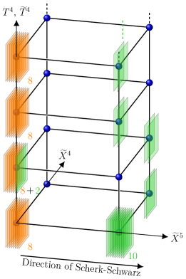
(a) Configuration in the component $({\cal R},\tilde{\cal R})=(0,8)$ of the moduli space, with $n_{\rm F}-n_{\rm B}=0$. The masses at one loop of two blowing-up moduli in the twisted closed-string sector of $T^{4}/\mathbb{Z}_{2}$ deserve further study.

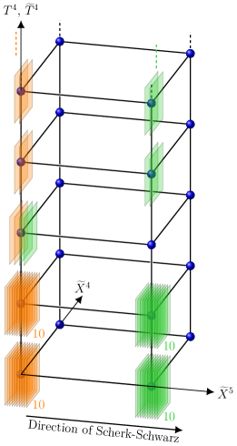
(b) Configuration in the component $({\cal R},\tilde{\cal R})=(8,8)$ of the moduli space, with $n_{\rm F}-n_{\rm B}=32$. All twisted-sector moduli are massive.

Figure 5: D3-brane configurations without tachyons at one loop in the NN, DD and ND+DN open-string sectors, as well as in the untwisted closed string sector.

As follows from the mass-term coefficients (7.188), all D3-brane postions along $T^{4}/\mathbb{Z}_{2}$ and $\tilde{T}^{4}/\mathbb{Z}_{2}$ turn out to be rigid or massive. By taking into account the Green–Schwarz mechanism which stabilizes automatically 14 linear combinations of continuous locations along $\tilde{T}^{2}$, the mass-matrix of the 18 remaining positions can be found and leads to the conclusion that they are all massless except one which is massive. As explained in the previous subsection, all untwisted closed-string moduli are flat directions, including $M_{3/2}$ thanks to the vanishing of $n_{\rm F}-n_{\rm B}$. The moduli in the ND+DN sectors are realized as strings “stretched” between the stack of 2 D3-branes T-dual to D9-branes located on the left side of Fig. 5(a) and any of the four stacks of 8 D3-branes T-dual to D5-branes. Indeed, they share the same coordinates in $\tilde{T}^{2}$. In all four cases, we have in the notations of Eqs. (6.180) and (6.181,

$$N_{i_{0}i^{\prime}_{0}}=2\,,\quad N_{i_{0}\hat{\imath}^{\prime}_{0}}=0\,,\quad D_{j_{0}i^{\prime}_{0}}=8\,,\quad D_{j_{0}\hat{\imath}^{\prime}_{0}}=0\,,$$ (7.191)

$$\Longrightarrow n_{i_{0}i_{0}^{\prime}}-n_{i_{0}\hat{\imath}_{0}^{\prime}}-1+d_{j_{0}i_{0}^{\prime}}-d_{j_{0}\hat{\imath}_{0}^{\prime}}-1=3>0\,,$$

which shows that all moduli fields in the ND+DN sector are massive.

For completeness, let us review the counting of $n_{\rm B}$ and $n_{\rm F}$. In the NN and DD sectors, the bosonic degrees of freedom include those of an ${\cal N}=2$ vector multiplet in the adjoint representation of the group (7.189), along with those of hypermultiplets in antisymmetric $\oplus$ $\overline{\text{antisymmetric}}$ representations of all non-Abelian factors. In the ND+DN sector, we have the bosonic degrees of freedom of 4 hypermultiplets, all transforming under a “bifundamental” representation of a $U(1)_{\rm NN}\times U(4)_{\rm DD}$ group. Adding the 96 degrees of freedom arising from the closed-string sector, we obtain a total of $n_{\rm B}=832$. On the contrary, $n_{\rm F}$ contains only contributions from the ND+DN sector. The latter correspond to the fermionic degrees of freedom of hypermultiplets in the bifundamental representations of each pair of unitary group factors supported by stacks of D3-branes T-dual to D5-branes and stacks of D3- branes T-dual to D9-branes, provided they have distinct coordinates along $\tilde{X}^{5}$ but not $\tilde{X}^{4}$. Their total number is given by $n_{\rm F}=4\times 16\times 13=832$, which equals $n_{\rm B}$ as claimed before.

Positive one-loop potential:

The second configuration we are interested in lies in the component $({\cal R},\tilde{\cal R})=(8,8)$ of the moduli space. It yields a positive potential satisfying $n_{\rm F}-n_{\rm B}=32$ and is depicted in Fig. 5(b). The D3-branes T-dual to the D5-branes are distributed in $T^{4}/\mathbb{Z}_{2}$ as 6 pairs and 2 stacks of 10. Similarly, the D3-branes T-dual to the D9-branes are located in $\tilde{T}^{4}/\mathbb{Z}_{2}$ as 6 pairs and 2 stacks of 10. Because the precise positions in $\tilde{T}^{2}$ shown in Fig. 5(b) do not involve the direction $\tilde{X}^{4}$, the configuration could be considered in five dimensions.

Including the anomalous $U(1)$’s, the open-string gauge group is

$$\left[U(1)^{6}\times U(5)^{2}\right]_{\rm DD}\times\left[U(1)^{6}\times U(5)^{2}\right]_{\rm NN}\,,$$ (7.192)

both in four and six dimensions. It contains 16 unitary factors, which implies that all twisted sector moduli are massive, i.e. that $T^{4}/\mathbb{Z}_{2}$ cannot be desingularized. Moreover, the anomaly-free gauge symmetry is reduced to

$$\left[SU(5)^{2}\right]_{\rm DD}\times\left[SU(5)^{2}\right]_{\rm NN}\,.$$ (7.193)

All D3-brane positions in $T^{4}/\mathbb{Z}_{2}$ or $\tilde{T}^{4}/\mathbb{Z}_{2}$ turn out to be rigid of massive at one loop, while the Green-Schwarz mechanism leaves $8$ massive and $8$ massless moduli associated with the locations in $\tilde{T}^{2}$. Moreover, all untwisted closed-string moduli are flat directions except the supersymmetry breaking scale $M_{3/2}$ which undergoes a runaway along a positive potential. There are moduli in the ND+DN sector arising from strings “stretched” between any stack of D3-branes T-dual to D5-branes and the pair of D3-branes T-dual to D9-branes located on the same edged of the box. They include 2 copies of scalars in “bifundamental” representations of $U(1)_{\rm NN}\times U(5)_{\rm DD}$ groups, and 6 copies in “bifundamental” representations of $U(1)_{\rm NN}\times U(1)_{\rm DD}$ groups. In the former case the moduli are stabilized since we have

$$N_{i_{0}i^{\prime}_{0}}=2\,,\quad N_{i_{0}\hat{\imath}^{\prime}_{0}}=0\,,\quad D_{j_{0}i^{\prime}_{0}}=10\,,\quad D_{j_{0}\hat{\imath}^{\prime}_{0}}=0\,,$$ (7.194)

$$\Longrightarrow n_{i_{0}i_{0}^{\prime}}-n_{i_{0}\hat{\imath}_{0}^{\prime}}-1+d_{j_{0}i_{0}^{\prime}}-d_{j_{0}\hat{\imath}_{0}^{\prime}}-1=4>0\,,$$

while in the latter case they remain massless since

$$N_{i_{0}i^{\prime}_{0}}=2\,,\quad N_{i_{0}\hat{\imath}^{\prime}_{0}}=0\,,\quad D_{j_{0}i^{\prime}_{0}}=2\,,\quad D_{j_{0}\hat{\imath}^{\prime}_{0}}=0\,,$$ (7.195)

$$\Longrightarrow n_{i_{0}i_{0}^{\prime}}-n_{i_{0}\hat{\imath}_{0}^{\prime}}-1+d_{j_{0}i_{0}^{\prime}}-d_{j_{0}\hat{\imath}_{0}^{\prime}}-1=0\,.$$

Finally, the counting of the classically massless degrees of freedom can be done as in the brane configuration of Fig. 5(a) and leads to $n_{\rm F}-n_{\rm B}=32$.

8 Conclusions

In this work, we have calculated the quadratic mass terms of the moduli fields arising in the ND+DN sector of the type IIB orientifold model compactified on $T^{2}\times T^{4}/\mathbb{Z}_{2}$, when ${\cal N}=2$ supersymmetry is spontaneously broken via the SSmechanism implemented along one direction of $T^{2}$. Assuming the string coupling is weak, this is done at one loop by computing the two-point functions of “boundary-changing vertex operators” inserted on the boundaries of the annulus and Möbius strip. The main difficulties of the derivation to which we have paid particular attention are the following:

• Using the stress-tensor method, the correlators of ground-state boundary-changing fields and spin fields are found up to “integration constants,” which are functions of the Teichmüller parameters of the double-cover tori. This leads to an ambiguity in the full amplitude of interest, which is lifted by taking the limit where the insertion points of the vertices coalesce. Indeed, the expression reduces in this case to contributions of the partition function that arise from states with specific Chan–Paton indices only. This very fact makes this step of the computation more involved than its counterpart for closed-string amplitudes of twisted-sector states for which this identification is made with the entire partition function.

• The two-point function can be split into two parts referred to as “external” and “internal.” The former, which is dressed by a kinematic factor, can be used to derive the one-loop correction to the Kähler metric and involves only correlation functions of “ground-state boundary-changing fields.” By contrast, the internal part which captures the mass correction also requires correlators of “excited boundary-changing fields”. These extra ingredients contain two contributions: One arises from periodicity properties of the orbifold-background coordinates, and the other from pure local monodromy effects. Although the latter have often been neglected in favor of the former in the literature, both turn out to be of equal order of magnitude, as we have shown explicitly.

The squared masses of all moduli fields have been derived at one loop and up to contributions that are suppressed when $M_{3/2}$ is lower than the other scales of the background. When the results are strictly positive, the corresponding scalars can be stabilized dynamically during the cosmological evolution of the universe [66, 67, 68, 69, 70, 38, 71] in the regions in moduli space compatible with weak coupling and the assumption on $M_{3/2}$. However the potentially dominant contributions to the mass terms of moduli in the NN, DD or ND+DN open-string sectors can accidentally vanish for certain brane configurations. In such cases, the issue of quartic interactions potentially inducing instabilities of the backgrounds arises. The fact that the untwisted closed-string moduli $(G+C)_{I^{\prime}J^{\prime}}$ and $(G+C)_{IJ}$ are flat directions (up to exponentially suppressed corrections) seems to be a more severe difficulty. However, heterotic/type I duality can be used to show that non-perturbative contributions of D1-branes, which are captured by a one-loop computation of the effective potential on the heterotic side, can stabilize some of these moduli [72, 38, 73, 74]. However, for large SSdirection i.e. small $M_{3/2}\equiv M_{\rm s}\sqrt{G^{55}}/2$ compared to $M_{\rm s}$, this mechanism is ineffective for the components $(G+C)_{5J}$ and $(G+C)_{5J^{\prime}}$ (which include the degree of freedom of $M_{3/2}$ itself) for which extra physics should be invoked to yield their stabilization.

Appendix A Conventions of matrix actions on Chan–Paton indices

In Ref. [5], the actions of the group elements $G\in\{1,g,\Omega,\Omega g\}$ on the Dirichlet or Neumann Chan–Paton indices $\alpha\in\{1,\dots,32\}$ are always represented by $32\times 32$ matrices. If needed, they define traces with an index $I$ (that would be denoted $i$ in our notations) labelling a fixed point of $T^{4}/\mathbb{Z}_{2}$ to indicate when they restrict to the matrix entries associated with the fixed point $I$ (see their Eq. (2.22)). In our conventions, we work directly with smaller matrices, one for each fixed point $ii^{\prime}$ of $\tilde{T}^{2}\times T^{4}/\mathbb{Z}_{2}$ or $\tilde{T}^{2}\times\tilde{T}^{4}/\mathbb{Z}_{2}$, which are submatrices of those used in Ref. [5]. In this appendix, we would like to give a detailed correspondance between their notations and ours for the traces appearing in the open-string contributions to the partition function.

Let us focus on the matrices acting on the Neumann Chan–Paton factors. In order to avoid any ambiguity, we first define the sets of indices ${\cal H}_{ii^{\prime}}$ associated with the fixed points $ii^{\prime}$ that are used to generate the submatrices from the big ones. To this end, we label the fixed points in lexicographical order, $\left(11,12,13,14,21,\dots\right)$, and introduce a function $p(i,i^{\prime})$ that gives the predecessor in this list,

$$p(i,i^{\prime})=\left\{\!\begin{array}[]{ll}i,i^{\prime}-1&\text{ if }i^{\prime}\in\{2,3,4\}\\ i-1,4&\text{ if }i^{\prime}=1\phantom{{{L^{L}}^{L}}^{L}}\end{array}\right.\!\!.$$ (A.196)

The sets are then

$${\cal H}_{11}=\left\{\!\begin{array}[]{l}\varnothing\leavevmode\nobreak\ \leavevmode\nobreak\ \leavevmode\nobreak\ \text{ if }N_{11}=0\\ \left\{1,\dots,\frac{N_{11}}{2}\right\}\cup\left\{17,\dots,16+\frac{N_{11}}{2}\right\}\leavevmode\nobreak\ \leavevmode\nobreak\ \text{ if }N_{11}\neq 0\end{array}\right.\!\!,$$ (A.197)

and for $ii^{\prime}\neq 11$,

$${\cal H}_{ii^{\prime}}=\left\{\!\begin{array}[]{l}\varnothing\leavevmode\nobreak\ \leavevmode\nobreak\ \leavevmode\nobreak\ \text{ if }N_{ii^{\prime}}=0\\ \left\{\frac{N_{p(i,i^{\prime})}}{2}+1,\dots,\frac{N_{p(i,i^{\prime})}}{2}+\frac{N_{ii^{\prime}}}{2}\right\}\cup\left\{\frac{N_{p(i,i^{\prime})}}{2}+17,\dots,16+\frac{N_{p(i,i^{\prime})}}{2}+\frac{N_{ii^{\prime}}}{2}\right\}\leavevmode\nobreak\ \leavevmode\nobreak\ \text{ if }N_{ii^{\prime}}\neq 0\end{array}\right.\!\!.$$ (A.198)

Our $N_{ii^{\prime}}\times N_{ii^{\prime}}$ matrices $\gamma_{{\rm N},G}^{ii^{\prime}}$ are formed from $32\times 32$ matrices $\gamma_{{\rm N},G}$ as follows,

$$\gamma_{{\rm N},G}^{ii^{\prime}}=\gamma_{{\rm N},G}|_{{}_{{\cal H}_{ii^{\prime}}}}\,,$$ (A.199)

where the notation in the right-hand side means that we form submatrices by keeping the rows and columns $\alpha\in{\cal H}_{ii^{\prime}}$. The traces of $32\times 32$ matrices can then be expressed as

$$\textrm{tr}(\gamma_{{\rm N},G}) =\sum_{\alpha=1}^{32}(\gamma_{{\rm N},G})_{\alpha\alpha}=\sum_{i,i^{\prime}}\sum_{\alpha\in{\cal H}_{ii^{\prime}}}(\gamma_{{\rm N},G})_{\alpha\alpha}=\sum_{i,i^{\prime}}\textrm{tr}(\gamma_{{\rm N},G}|_{{}_{{\cal H}_{ii^{\prime}}}})$$ (A.200)

$$=\sum_{i,i^{\prime}}\textrm{tr}(\gamma_{{\rm N},G}^{ii^{\prime}})\,,$$

and similarly for the matrices associated with the Dirichlet sector.

Moreover, in order to justify the replacement (2.16), let us define in our notations the $32\times 32$ matrix ${\cal W}_{j}$ that is denoted $W_{I}$ and appears in Eq. (2.22) of Ref. [5],

$${\cal W}_{j}=\prod_{I=6}^{9}{\cal W}_{I}^{2a^{I}_{j}}\,,\quad\mbox{where}\quad{\cal W}_{I}=I_{2}\otimes\begin{pmatrix}e^{2i\pi a_{1}^{I}}I_{\frac{N_{1}}{2}}&&{}_{\text{\Large{0}}}\\ &\ddots&\\ {}^{\text{\Large{0}}}&&e^{2i\pi a_{16}^{I}}I_{\frac{N_{16}}{2}}\end{pmatrix},\quad N_{i}\equiv\sum_{i^{\prime}}N_{ii^{\prime}}\,.$$ (A.201)

For $G=g$ we have to compute

$$\textrm{tr}({\cal W}_{j}\gamma_{{\rm N},g}) =\sum_{\alpha=1}^{32}({\cal W}_{j}\gamma_{{\rm N},g})_{\alpha\alpha}=\sum_{\alpha=1}^{32}\sum_{\beta=1}^{32}({\cal W}_{j})_{\alpha\beta}(\gamma_{{\rm N},g})_{\beta\alpha}=\sum_{\alpha=1}^{32}({\cal W}_{j})_{\alpha\alpha}(\gamma_{{\rm N},g})_{\alpha\alpha}$$ (A.202)

$$=\sum_{i,i^{\prime}}\sum_{\alpha\in{\cal H}_{ii^{\prime}}}({\cal W}_{j})_{\alpha\alpha}(\gamma_{{\rm N},g})_{\alpha\alpha}=\sum_{i,i^{\prime}}e^{4i\pi\vec{a}_{i}\cdot\vec{a}_{j}}\sum_{\alpha\in{\cal H}_{ii^{\prime}}}(\gamma_{{\rm N},g})_{\alpha\alpha}$$

$$=\sum_{i,i^{\prime}}e^{4i\pi\vec{a}_{i}\cdot\vec{a}_{j}}\textrm{tr}(\gamma_{{\rm N},g}^{ii^{\prime}})\,.$$

In this derivation, we have used the fact that the matrix ${\cal W}_{j}$ is diagonal and that its components $\alpha\alpha$ for $\alpha\in{\cal H}_{ii^{\prime}}$ are $e^{4i\pi\vec{a}_{i}\cdot\vec{a}_{j}}$.

Appendix B Closed-string sector partition function

In this appendix, we display the closed-string contributions to the one-loop partition function defined in Eq. (2.9).

In order to write $Z_{\cal T}$, we introduce the lattices of zero modes of the bosonic coordinates associated with $T^{4}$ and $T^{2}$,

$$\Lambda_{\vec{m},\vec{n}}^{(4,4)}(\tau)\,=q^{{1\over 4}P^{\rm L}_{I}G^{IJ}P^{\rm L}_{J}}\,\bar{q}^{{1\over 4}P^{\rm R}_{I}G^{IJ}P^{\rm R}_{J}}\,, P^{\rm L}_{I}=m_{I}+G_{IJ}n_{J}\,, P^{\rm R}_{I}=m_{I}-G_{IJ}n_{J}\,,$$ (B.203)

$$\Lambda_{\vec{m}^{\prime},\vec{n}^{\prime}}^{(2,2)}(\tau)=q^{{1\over 4}P^{\rm L}_{I^{\prime}}G^{I^{\prime}J^{\prime}}P^{\rm L}_{J^{\prime}}}\,\bar{q}^{{1\over 4}P^{\rm R}_{I^{\prime}}G^{I^{\prime}J^{\prime}}P^{\rm R}_{J^{\prime}}}\,, P^{\rm L}_{I^{\prime}}=m_{I^{\prime}}+G_{I^{\prime}J^{\prime}}n_{J^{\prime}}\,, P^{\rm R}_{I^{\prime}}=m_{I^{\prime}}-G_{I^{\prime}J^{\prime}}n_{J^{\prime}}\,,$$

where $\vec{m}$, $\vec{n}$ and $\vec{m}^{\prime}$, $\vec{n}^{\prime}$ are four-vectors and two-vectors whose components are integer momenta and winding numbers.

Moreover, the worldsheet fermions generate an $SO(8)$ affine symmetry broken to $SO(4)\times SO(4)$ by the $\mathbb{Z}_{2}$-orbifold action. As a result, their contributions to the partition function take the forms of ordered pairs of characters of $SO(4)$. The latter can be expressed in terms of Jacobi modular forms and the Dedekind function,

$$\vartheta\big{[}{}^{\alpha}_{\beta}\big{]}(z|\tau)=\sum_{k\in\mathbb{Z}}q^{{1\over 2}(k+\alpha)^{2}}e^{2i\pi(z+\beta)(k+\alpha)}\,,\leavevmode\nobreak\ \leavevmode\nobreak\ \quad\eta(\tau)=q^{1\over 24}\prod_{n=1}^{+\infty}(1-q^{n})\,,\leavevmode\nobreak\ \leavevmode\nobreak\ \quad q=e^{2i\pi\tau}\,.$$ (B.204)

Denoting as usual

$$\vartheta\big{[}{}^{0}_{0}\big{]}(z|\tau)\equiv\vartheta_{3}(z|\tau)\,,\leavevmode\nobreak\ \leavevmode\nobreak\ \vartheta\Big{[}{}^{{}^{\scriptstyle\phantom{.}\!0}}_{1\over 2}\Big{]}(z|\tau)\equiv\vartheta_{4}(z|\tau)\,,\leavevmode\nobreak\ \leavevmode\nobreak\ \vartheta\Big{[}{}^{1\over 2}_{\phantom{\!|}{}_{\scriptstyle 0}}\Big{]}(z|\tau)\equiv\vartheta_{2}(z|\tau)\,,\leavevmode\nobreak\ \leavevmode\nobreak\ \vartheta\Big{[}{}^{1\over 2}_{1\over 2}\Big{]}(z|\tau)\equiv\vartheta_{1}(z|\tau)\,,$$ (B.205)

the characters are given by [55, 56, 57]

$$O_{4}=\frac{\vartheta_{3}^{2}+\vartheta_{4}^{2}}{2\eta^{2}}\,,\quad\leavevmode\nobreak\ \leavevmode\nobreak\ V_{4}=\frac{\vartheta_{3}^{2}-\vartheta_{4}^{2}}{2\eta^{2}}\,,\quad\leavevmode\nobreak\ \leavevmode\nobreak\ S_{4}=\frac{\vartheta_{2}^{2}+i^{-2}\vartheta_{1}^{2}}{2\eta^{2}}\,,\quad\leavevmode\nobreak\ \leavevmode\nobreak\ C_{4}=\frac{\vartheta_{2}^{2}-i^{-2}\vartheta_{1}^{2}}{2\eta^{2}}\,,$$ (B.206)

where it is understood that $\vartheta_{n}\equiv\vartheta_{n}(0|\tau)$.

Given these notations, the torus contribution to the partition function takes the following form,

$$Z_{\cal T}={1\over 4}\,{1\over\tau_{2}^{2}}\,\bigg{\{}\bigg{[}\left(\left|V_{4}O_{4}+O_{4}V_{4}\right|^{2}+\left|S_{4}S_{4}+C_{4}C_{4}\right|^{2}\right)\sum_{\vec{m},\vec{n}}\frac{\Lambda^{(4,4)}_{\vec{m},\vec{n}}}{\left|\eta^{4}\right|^{2}}$$

$$+\left(\left|V_{4}O_{4}-O_{4}V_{4}\right|^{2}+\left|S_{4}S_{4}-C_{4}C_{4}\right|^{2}\right)\left|\frac{2\eta}{\vartheta_{2}}\right|^{4}$$

$$+16\left(\left|O_{4}C_{4}+V_{4}S_{4}\right|^{2}+\left|S_{4}O_{4}+C_{4}V_{4}\right|^{2}\right)\left|\frac{\eta}{\vartheta_{4}}\right|^{4}$$

$$+16\left(\left|O_{4}C_{4}-V_{4}S_{4}\right|^{2}+\left|S_{4}O_{4}-C_{4}V_{4}\right|^{2}\right)\left|\frac{\eta}{\vartheta_{3}}\right|^{4}\bigg{]}\sum_{\vec{m}^{\prime},\vec{n}^{\prime}}\frac{\Lambda^{(2,2)}_{\vec{m}^{\prime},(n_{4},2n_{5})}}{\left|\eta^{4}\right|^{2}}$$

$$-\bigg{[}\left((V_{4}O_{4}+O_{4}V_{4})(\bar{S}_{4}\bar{S}_{4}+\bar{C}_{4}\bar{C}_{4})+(S_{4}S_{4}+C_{4}C_{4})(\bar{V}_{4}\bar{O}_{4}+\bar{O}_{4}\bar{V}_{4})\right)\sum_{\vec{m},\vec{n}}\frac{\Lambda^{(4,4)}_{\vec{m},\vec{n}}}{\left|\eta^{4}\right|^{2}}$$

$$+\left((V_{4}O_{4}-O_{4}V_{4})(\bar{S}_{4}\bar{S}_{4}-\bar{C}_{4}\bar{C}_{4})+(S_{4}S_{4}-C_{4}C_{4})(\bar{V}_{4}\bar{O}_{4}-\bar{O}_{4}\bar{V}_{4})\right)\left|\frac{2\eta}{\vartheta_{2}}\right|^{4}$$

$$+16\left((O_{4}C_{4}+V_{4}S_{4})(\bar{S}_{4}\bar{O}_{4}+\bar{C}_{4}\bar{V}_{4})+(S_{4}O_{4}+C_{4}V_{4})(\bar{O}_{4}\bar{C}_{4}+\bar{V}_{4}\bar{S}_{4})\right)\left|\frac{\eta}{\vartheta_{4}}\right|^{4}$$ (B.207)

$$+16\left((O_{4}C_{4}-V_{4}S_{4})(\bar{S}_{4}\bar{O}_{4}-\bar{C}_{4}\bar{V}_{4})+(S_{4}O_{4}-C_{4}V_{4})(\bar{O}_{4}\bar{C}_{4}-\bar{V}_{4}\bar{S}_{4})\right)\left|\frac{\eta}{\vartheta_{3}}\right|^{4}\bigg{]}\sum_{\vec{m}^{\prime},\vec{n}^{\prime}}\frac{\Lambda^{(2,2)}_{\vec{m}^{\prime}+\vec{a}^{\prime}_{\text{S}},(n_{4},2n_{5})}}{\left|\eta^{4}\right|^{2}}$$

$$+\bigg{[}\left(\left|O_{4}O_{4}+V_{4}V_{4}\right|^{2}+\left|C_{4}S_{4}+S_{4}C_{4}\right|^{2}\right)\sum_{\vec{m},\vec{n}}\frac{\Lambda^{(4,4)}_{\vec{m},\vec{n}}}{\left|\eta^{4}\right|^{2}}+\left(\left|O_{4}O_{4}-V_{4}V_{4}\right|^{2}+\left|S_{4}C_{4}-C_{4}S_{4}\right|^{2}\right)\left|\frac{2\eta}{\vartheta_{2}}\right|^{4}$$

$$+16\left(\left|O_{4}S_{4}+V_{4}C_{4}\right|^{2}+\left|S_{4}V_{4}+C_{4}O_{4}\right|^{2}\right)\left|\frac{\eta}{\vartheta_{4}}\right|^{4}$$

$$+16\left(\left|O_{4}S_{4}-V_{4}C_{4}\right|^{2}+\left|S_{4}V_{4}-C_{4}O_{4}\right|^{2}\right)\left|\frac{\eta}{\vartheta_{3}}\right|^{4}\bigg{]}\sum_{\vec{m}^{\prime},\vec{n}^{\prime}}\frac{\Lambda^{(2,2)}_{\vec{m}^{\prime},(n_{4},2n_{5}+1)}}{\left|\eta^{4}\right|^{2}}$$

$$-\bigg{[}\left((O_{4}O_{4}+V_{4}V_{4})(\bar{C}_{4}\bar{S}_{4}+\bar{S}_{4}\bar{C}_{4})+(C_{4}S_{4}+S_{4}C_{4})(\bar{O}_{4}\bar{O}_{4}+\bar{V}_{4}\bar{V}_{4})\right)\sum_{\vec{m},\vec{n}}\frac{\Lambda^{(4,4)}_{\vec{m},\vec{n}}}{\left|\eta^{4}\right|^{2}}$$

$$+\left((O_{4}O_{4}-V_{4}V_{4})(\bar{S}_{4}\bar{C}_{4}-\bar{C}_{4}\bar{S}_{4})+(S_{4}C_{4}-C_{4}S_{4})(\bar{O}_{4}\bar{O}_{4}-\bar{V}_{4}\bar{V}_{4})\right)\left|\frac{2\eta}{\vartheta_{2}}\right|^{4}$$

$$+16\left((O_{4}S_{4}+V_{4}C_{4})(\bar{S}_{4}\bar{V}_{4}+\bar{C}_{4}\bar{O}_{4})+(S_{4}V_{4}+C_{4}O_{4})(\bar{O}_{4}\bar{S}_{4}+\bar{V}_{4}\bar{C}_{4})\right)\left|\frac{\eta}{\vartheta_{4}}\right|^{4}$$

$$+16\left((O_{4}S_{4}-V_{4}C_{4})(\bar{S}_{4}\bar{V}_{4}-\bar{C}_{4}\bar{O}_{4})+(S_{4}V_{4}-C_{4}O_{4})(\bar{O}_{4}\bar{S}_{4}-\bar{V}_{4}\bar{C}_{4})\right)\left|\frac{\eta}{\vartheta_{3}}\right|^{4}\bigg{]}\sum_{\vec{m}^{\prime},\vec{n}^{\prime}}\frac{\Lambda^{(2,2)}_{\vec{m}^{\prime}+\vec{a}_{\rm S}^{\prime},(n_{4},2n_{5}+1)}}{\left|\eta^{4}\right|^{2}}\bigg{\}},$$

where the momenta $\vec{m}^{\prime}$ of all fermionic degrees of freedom are shifted as shown in Eq. (2.6).

The expression of the Klein-bottle contribution to the partition function involves only left-right symmetric states which are therefore bosonic. As a result it is identical to that found in the supersymmetric model of Sect. 2.1,

$$Z_{\cal K}= {1\over 4}\,{1\over\tau_{2}^{2}}\,\bigg{\{}\left(V_{4}O_{4}+O_{4}V_{4}\right)\bigg{(}\sum_{\vec{m}}\frac{P^{(4)}_{\vec{m}}}{\eta^{4}}+\sum_{\vec{n}}\frac{W^{(4)}_{\vec{n}}}{\eta^{4}}\bigg{)}+32\left(O_{4}C_{4}+V_{4}S_{4}\right)\left(\frac{\eta}{\vartheta_{4}}\right)^{2}$$ (B.208)

$$-\left(S_{4}S_{4}+C_{4}C_{4}\right)\bigg{(}\sum_{\vec{m}}\frac{P^{(4)}_{\vec{m}}}{\eta^{4}}+\sum_{\vec{n}}\frac{W^{(4)}_{\vec{n}}}{\eta^{4}}\bigg{)}-32\left(S_{4}O_{4}+C_{4}V_{4}\right)\left(\frac{\eta}{\vartheta_{4}}\right)^{2}\bigg{\}}\sum_{\vec{m}^{\prime}}\frac{P^{(2)}_{\vec{m}^{\prime}}}{\eta^{4}}\,,$$

where all lattices are identical to those defined in the open-string sector, Eqs. (2.11) and (2.12), and the characters and modular forms are evaluated at $2i\tau_{2}$.

Appendix C Leading behavior of $\varepsilon$ when $\alpha^{\prime}\to 0$

In this appendix, we reconsider the small $\alpha^{\prime}$ limit of the roots $U_{1}$ of $\Omega(U)$ for arbitrary $|{\rm Im}\,Y_{1}|<\frac{1}{2}\,{\rm Im}\,\tau^{\rm dc}$, which are given in Eq. (6.139). Our goal is to find the leading behavior of $\varepsilon$.

Using the full expansion of $\vartheta_{1}(z)$ given in Eq. (6.120), one obtains

$${\vartheta_{1}^{\prime}\over\vartheta_{1}}(z)=\pi\cot(\pi z)+2i\pi\sum_{n\geq 1}\big{[}H(q_{\rm dc}^{n}\,e^{-2i\pi z})-H(q_{\rm dc}^{n}\,e^{2i\pi z})\big{]}\,,\quad H(z)\equiv{z\over 1-z}\,,$$ (C.209)

which can be used to rewrite the equation $\Omega(U_{1})=0$ as follows,

$$i\sin(\pi Y_{1})=2\sin(\pi U_{1})\sin[\pi(Y_{1}-U_{1})]\,\sum_{n\geq 1} \Big{[}H\big{(}q_{\rm dc}^{n}\,e^{-2i\pi U_{1}}\big{)}-H\big{(}q_{\rm dc}^{n}\,e^{2i\pi U_{1}}\big{)}$$ (C.210)

$$\!\!\!\!\!+H\big{(}q_{\rm dc}^{n}\,e^{-2i\pi(Y_{1}-U_{1})}\big{)}-H\big{(}q_{\rm dc}^{n}\,e^{2i\pi(Y_{1}-U_{1})}\big{)}\Big{]}\,.$$

Applying the change of variable given in Eq. (6.139), the above expression becomes

$$i\sin(\pi Y_{1})= \;\frac{1}{2}\big{(}1-(-1)^{m}\,i\,e^{i\pi(\tau^{\rm dc}+Y_{1})}\,e^{2i\pi\varepsilon}\big{)}\big{(}1-(-1)^{m}\,i\,e^{i\pi(\tau^{\rm dc}-Y_{1})}\,e^{2i\pi\varepsilon}\big{)}\,e^{-2i\pi\varepsilon}\phantom{\!\!\underset{\displaystyle|}{\cdot}}$$

$$\times\!\Bigg{\{}\!-{e^{-i\pi Y_{1}}\,e^{-2i\pi\varepsilon}\over 1+(-1)^{m}\,i\,e^{i\pi(\tau^{\rm dc}-Y_{1})}\,e^{-2i\pi\varepsilon}}$$ (C.211)

$$\leavevmode\nobreak\ \leavevmode\nobreak\ \leavevmode\nobreak\ \leavevmode\nobreak\ \leavevmode\nobreak\ +2i\sum_{n\geq 1}{q_{\rm dc}^{n}\,e^{-i\pi Y_{1}}\big{(}\sin(2\pi\varepsilon)+(-1)^{m}\,q_{\rm dc}^{n}\,e^{i\pi(\tau^{\rm dc}-Y_{1})}\big{)}\over\big{(}1+(-1)^{m}\,i\,q_{\rm dc}^{n}\,e^{i\pi(\tau^{\rm dc}-Y_{1})}\,e^{-2i\pi\varepsilon}\big{)}\big{(}1-(-1)^{m}\,i\,q_{\rm dc}^{n}\,e^{i\pi(\tau^{\rm dc}-Y_{1})}\,e^{2i\pi\varepsilon}\big{)}}$$

$$\leavevmode\nobreak\ \leavevmode\nobreak\ \leavevmode\nobreak\ \leavevmode\nobreak\ \leavevmode\nobreak\ -(Y_{1}\to-Y_{1})\Bigg{\}}\,,$$

where the first term in the braces and its transformed under $Y_{1}\to-Y_{1}$ arise from the contributions $n=1$ of the first and fourth functions $H$ in Eq. (C.210).

• If $0<{\rm Im}\,Y_{1}<\frac{1}{2}\,{\rm Im}\,\tau^{\rm dc}$, and assuming $\varepsilon\to 0$ when $\alpha^{\prime}\to 0$, Eq. (C.211) reads

  $$(e^{2i\pi Y_{1}}-1)\,e^{-i\pi Y_{1}}= \,\big{(}1-2i\pi\varepsilon-(-1)^{m}\,i\,e^{i\pi(\tau^{\rm dc}-Y_{1})}+\mbox{sub dom.}\big{)}$$ (C.212)

  $$\,\Big{\{}-e^{-i\pi Y_{1}}\big{(}1-2i\pi\varepsilon-(-1)^{m}\,i\,e^{i\pi(\tau^{\rm dc}-Y_{1})}+\mbox{sub dom.}\big{)}$$

  $$\,\leavevmode\nobreak\ \leavevmode\nobreak\ +e^{i\pi Y_{1}}\big{(}1-2i\pi\varepsilon-(-1)^{m}\,i\,e^{i\pi(\tau^{\rm dc}+Y_{1})}+\mbox{sub dom.}\big{)}\Big{\}}\,,$$

  where all contributions $n\geq 1$ have been absorbed in “subdominant” contributions. Simplifying this expression, one obtains

  $$0=4i\pi\varepsilon+2(-1)^{m}\,i\,e^{i\pi(\tau^{\rm dc}-Y_{1})}+\mbox{subdom.}\,,$$ (C.213)

  which leads to the asymptotics

  $$\varepsilon\underset{\alpha^{\prime}\to 0}{\sim}-{(-1)^{m}\over 2\pi}\,e^{i\pi(\tau^{\rm dc}-Y_{1})}\underset{\alpha^{\prime}\to 0}{\longrightarrow}0\,.$$ (C.214)

  Our assumption on the convergence of $\varepsilon$ being consistent, we have shown the existence of solutions $U_{1}$ with the above behavior.

• If $-\frac{1}{2}\,{\rm Im}\,\tau^{\rm dc}<{\rm Im}\,Y_{1}<0$, Eq. (C.211) being invariant under $Y_{1}\to-Y_{1}$, one obtains immediately from the previous analysis that

  $$\varepsilon\underset{\alpha^{\prime}\to 0}{\sim}-{(-1)^{m}\over 2\pi}\,e^{i\pi(\tau^{\rm dc}+Y_{1})}\underset{\alpha^{\prime}\to 0}{\longrightarrow}0\,.$$ (C.215)

References

- [1] L. J. Dixon, D. Friedan, E. J. Martinec and S. H. Shenker, “The conformal field theory of orbifolds,” Nucl. Phys. B 282 (1987) 13.
- [2] J. J. Atick, L. J. Dixon, P. A. Griffin and D. Nemeschansky, “Multiloop twist field correlation functions for orbifolds,” Nucl. Phys. B 298 (1988) 1.
- [3] M. Bianchi and A. Sagnotti, “Twist symmetry and open string Wilson lines,” Nucl. Phys. B 361 (1991) 519.
- [4] E. G. Gimon and J. Polchinski, “Consistency conditions for orientifolds and D-manifolds,” Phys. Rev. D 54 (1996) 1667 [hep-th/9601038].
- [5] M. Berkooz, R. G. Leigh, J. Polchinski, J. H. Schwarz, N. Seiberg and E. Witten, “Anomalies, dualities, and topology of superstring vacua,” Nucl. Phys. B 475 (1996) 115 [hep-th/9605184].
- [6] A. Hashimoto, “Dynamics of Dirichlet-Neumann open strings on D-branes,” Nucl. Phys. B 496 (1997), 243-258 [arXiv:hep-th/9608127 [hep-th]].
- [7] C. P. Burgess and T. R. Morris, “Open and unoriented strings à la Polyakov,” Nucl. Phys. B 291 (1987), 256-284.
- [8] C. P. Burgess and T. R. Morris, “Open superstrings à la Polyakov,” Nucl. Phys. B 291 (1987), 285-333.
- [9] M. Cvetic and I. Papadimitriou, “Conformal field theory couplings for intersecting D-branes on orientifolds,” Phys. Rev. D 68 (2003), 046001 [erratum: Phys. Rev. D 70 (2004), 029903] [arXiv:hep-th/0303083 [hep-th]].
- [10] S. A. Abel and A. W. Owen, “Interactions in intersecting brane models,” Nucl. Phys. B 663 (2003), 197-214 [arXiv:hep-th/0303124 [hep-th]].
- [11] S. A. Abel and A. W. Owen, “-point amplitudes in intersecting brane models,” Nucl. Phys. B 682 (2004), 183-216 [arXiv:hep-th/0310257 [hep-th]].
- [12] P. Anastasopoulos, M. D. Goodsell and R. Richter, “Three- and four-point correlators of excited bosonic twist fields,” JHEP 10 (2013), 182 [arXiv:1305.7166 [hep-th]].
- [13] S. A. Abel and B. W. Schofield, “One-loop Yukawas on intersecting branes,” JHEP 06 (2005), 072 [arXiv:hep-th/0412206 [hep-th]].
- [14] B. Schofield, “One-loop phenomenology in brane models,” Durham thesis, Durham University, Ph.D. Thesis.
- [15] S. A. Abel and M. D. Goodsell, “Intersecting brane worlds at one loop,” JHEP 02 (2006), 049 [arXiv:hep-th/0512072 [hep-th]].
- [16] S. A. Abel and M. D. Goodsell, “Realistic Yukawa couplings through instantons in intersecting brane worlds,” JHEP 10 (2007), 034 [arXiv:hep-th/0612110 [hep-th]].
- [17] M. D. Goodsell, “One loop phenomenology of type II string theory: intersecting -branes and noncommutativity,” Durham thesis, Durham University, Ph.D. Thesis.
- [18] K. Benakli and M. D. Goodsell, “Two-point functions of chiral fields at one loop in Type II,” Nucl. Phys. B 805 (2008), 72-103 [arXiv:0805.1874 [hep-th]].
- [19] J. Frohlich, O. Grandjean, A. Recknagel and V. Schomerus, “Fundamental strings in D - D brane systems,” Nucl. Phys. B 583 (2000), 381-410 [arXiv:hep-th/9912079 [hep-th]].
- [20] P. Anastasopoulos, M. Bianchi and R. Richter, “On closed-string twist-field correlators and their open-string descendants,” [arXiv:1110.5359 [hep-th]].
- [21] L. Mattiello and I. Sachs, “ boundary twist fields and the moduli space of D-branes,” JHEP 07 (2018), 099 [arXiv:1803.07500 [hep-th]].
- [22] J. D. Blum and K. R. Dienes, “Duality without supersymmetry: The Case of the string,” Phys. Lett. B 414 (1997) 260 [hep-th/9707148].
- [23] J. D. Blum and K. R. Dienes, “Strong / weak coupling duality relations for nonsupersymmetric string theories,” Nucl. Phys. B 516 (1998) 83 [hep-th/9707160].
- [24] I. Antoniadis, E. Dudas and A. Sagnotti, “Supersymmetry breaking, open strings and M-theory,” Nucl. Phys. B 544 (1999) 469 [hep-th/9807011].
- [25] I. Antoniadis, G. D’Appollonio, E. Dudas and A. Sagnotti, “Partial breaking of supersymmetry, open strings and M-theory,” Nucl. Phys. B 553 (1999) 133 [hep-th/9812118].
- [26] I. Antoniadis, G. D’Appollonio, E. Dudas and A. Sagnotti, “Open descendants of freely acting orbifolds,” Nucl. Phys. B 565 (2000) 123 [hep-th/9907184].
- [27] A. L. Cotrone, “A orientifold with spontaneously broken supersymmetry,” Mod. Phys. Lett. A 14 (1999) 2487 [hep-th/9909116].
- [28] C. A. Scrucca and M. Serone, “On string models with Scherk–Schwarz supersymmetry breaking,” JHEP 0110 (2001) 017 [hep-th/0107159].
- [29] C. Angelantonj, M. Cardella and N. Irges, “Scherk–Schwarz breaking and intersecting branes,” Nucl. Phys. B 725 (2005) 115 [hep-th/0503179].
- [30] J. Scherk and J. H. Schwarz, “Spontaneous breaking of supersymmetry through dimensional reduction,” Phys. Lett. B 82 (1979) 60.
- [31] J. Scherk and J. H. Schwarz, “How to get masses from extra dimensions,” Nucl. Phys. B 153 (1979), 61-88.
- [32] S. Abel, T. Coudarchet and H. Partouche, “On the stability of open-string orbifold models with broken supersymmetry,” Nucl. Phys. B 957 (2020), 115100 [arXiv:2003.02545 [hep-th]].
- [33] S. Abel, E. Dudas, D. Lewis and H. Partouche, “Stability and vacuum energy in open string models with broken supersymmetry,” JHEP 1910 (2019) 226 [arXiv:1812.09714 [hep-th]].
- [34] H. Itoyama and T. R. Taylor, “Supersymmetry restoration in the compactified heterotic string theory,” Phys. Lett. B 186 (1987) 129.
- [35] S. Abel, K. R. Dienes and E. Mavroudi, “Towards a non-supersymmetric string phenomenology,” Phys. Rev. D 91 (2015) 126014 [arXiv:1502.03087 [hep-th]].
- [36] C. Kounnas and H. Partouche, “Super no-scale models in string theory,” Nucl. Phys. B 913 (2016) 593 [arXiv:1607.01767 [hep-th]].
- [37] C. Kounnas and H. Partouche, “ super no-scale models and moduli quantum stability,” Nucl. Phys. B 919 (2017) 41 [arXiv:1701.00545 [hep-th]].
- [38] T. Coudarchet and H. Partouche, “Quantum no-scale regimes and moduli dynamics,” Nucl. Phys. B 933 (2018) 134 [arXiv:1804.00466 [hep-th]].
- [39] I. Florakis and J. Rizos, “Chiral heterotic strings with positive cosmological constant,” Nucl. Phys. B 913 (2016) 495 [arXiv:1608.04582 [hep-th]].
- [40] S. Abel and R. J. Stewart, “On exponential suppression of the cosmological constant in non-SUSY strings at two loops and beyond,” Phys. Rev. D 96 (2017) 106013 [arXiv:1701.06629 [hep-th]].
- [41] S. Abel, K. R. Dienes and E. Mavroudi, “GUT precursors and entwined SUSY: The phenomenology of stable nonsupersymmetric strings,” Phys. Rev. D 97 (2018) no.12, 126017 [arXiv:1712.06894 [hep-ph]].
- [42] H. Itoyama and S. Nakajima, “Exponentially suppressed cosmological constant with enhanced gauge symmetry in heterotic interpolating models,” PTEP 2019 (2019) no.12, 123B01 [arXiv:1905.10745 [hep-th]].
- [43] H. Itoyama and S. Nakajima, “Stability, enhanced gauge symmetry and suppressed cosmological constant in 9D heterotic interpolating models,” Nucl. Phys. B 958 (2020), 115111 [arXiv:2003.11217 [hep-th]].
- [44] T. Coudarchet and H. Partouche, “Moduli stability in type I string orbifold models,” PoS CORFU2019 (2020), 164 [arXiv:2005.01764 [hep-th]].
- [45] J. Polchinski, “Tasi lectures on D-branes,” hep-th/9611050.
- [46] D. Cremades, L. E. Ibanez and F. Marchesano, “Intersecting brane models of particle physics and the Higgs mechanism,” JHEP 0207 (2002) 022 [hep-th/0203160].
- [47] D. Cremades, L. E. Ibanez and F. Marchesano, “Yukawa couplings in intersecting D-brane models,” JHEP 0307 (2003) 038 [hep-th/0302105].
- [48] B. Kors and P. Nath, “Effective action and soft supersymmetry breaking for intersecting D-brane models,” Nucl. Phys. B 681 (2004) 77 [hep-th/0309167].
- [49] D. Cremades, L. E. Ibanez and F. Marchesano, “Computing Yukawa couplings from magnetized extra dimensions,” JHEP 0405 (2004) 079 [hep-th/0404229].
- [50] R. Rohm, “Spontaneous supersymmetry breaking in supersymmetric string theories,” Nucl. Phys. B 237 (1984) 553.
- [51] C. Kounnas and M. Porrati, “Spontaneous supersymmetry breaking in string theory,” Nucl. Phys. B 310 (1988) 355.
- [52] S. Ferrara, C. Kounnas and M. Porrati, “Superstring solutions with spontaneously broken four-dimensional supersymmetry,” Nucl. Phys. B 304 (1988) 500.
- [53] S. Ferrara, C. Kounnas, M. Porrati and F. Zwirner, “Superstrings with spontaneously broken supersymmetry and their effective theories,” Nucl. Phys. B 318 (1989) 75.
- [54] C. Kounnas and B. Rostand, “Coordinate-dependent compactifications and discrete symmetries,” Nucl. Phys. B 341 (1990) 641.
- [55] W. Lerche, A. N. Schellekens and N. P. Warner, “Lattices and strings,” Phys. Rept. 177 (1989) 1.
- [56] W. Lerche, D. Lust and A. N. Schellekens, “Chiral four-dimensional heterotic strings from selfdual lattices,” Nucl. Phys. B 287 (1987) 477.
- [57] R. Blumenhagen, D. Lüst and S. Theisen, “Basic concepts of string theory,” Springer-Verlag, doi:10.1007/978-3-642-29497-6
- [58] C. Angelantonj and A. Sagnotti, “Open strings,” Phys. Rept. 371 (2002) 1 [Erratum-ibid. 376 (2003) 339] [arXiv:hep-th/0204089].
- [59] E. Dudas, “Theory and phenomenology of type I strings and M-theory,” Class. Quant. Grav. 17 (2000) R41 [arXiv:hep-ph/0006190].
- [60] D. Friedan, E. J. Martinec and S. H. Shenker, “Conformal Invariance, Supersymmetry and String Theory,” Nucl. Phys. B 271 (1986), 93-165.
- [61] I. Antoniadis, C. Bachas, C. Fabre, H. Partouche and T. R. Taylor, “Aspects of type I - type II - heterotic triality in four-dimensions,” Nucl. Phys. B 489 (1997) 160 [hep-th/9608012].
- [62] E. Kiritsis, “String theory in a nutshell,” Princeton University Press (2007) 588 p.
- [63] J. Polchinski, “String theory. Vol. 1: An introduction to the bosonic string,” Cambridge University Press (1998).
- [64] M. Dine and N. Seiberg, “Is the superstring weakly coupled?,” Phys. Lett. B 162 (1985), 299-302.
- [65] E. Cremmer, S. Ferrara, C. Kounnas and D. V. Nanopoulos, “Naturally vanishing cosmological constant in supergravity,” Phys. Lett. B 133 (1983) 61.
- [66] F. Bourliot, J. Estes, C. Kounnas and H. Partouche, “Cosmological phases of the string thermal effective potential,” Nucl. Phys. B 830 (2010) 330 [arXiv:0908.1881 [hep-th]].
- [67] J. Estes, C. Kounnas and H. Partouche, “Superstring cosmology for superstring vacua,” Fortsch. Phys. 59 (2011) 861 [arXiv:1003.0471 [hep-th]].
- [68] T. Catelin-Jullien, C. Kounnas, H. Partouche and N. Toumbas, “Induced superstring cosmologies and moduli stabilization,” Nucl. Phys. B 820 (2009) 290 [arXiv:0901.0259 [hep-th]].
- [69] F. Bourliot, C. Kounnas and H. Partouche, “Attraction to a radiation-like era in early superstring cosmologies,” Nucl. Phys. B 816 (2009) 227 [arXiv:0902.1892 [hep-th]].
- [70] T. Catelin-Jullien, C. Kounnas, H. Partouche and N. Toumbas, “Thermal/quantum effects and induced superstring cosmologies,” Nucl. Phys. B 797 (2008) 137 [arXiv:0710.3895 [hep-th]].
- [71] T. Coudarchet, C. Fleming and H. Partouche, “Quantum no-scale regimes in string theory,” Nucl. Phys. B 930 (2018) 235 [arXiv:1711.09122 [hep-th]].
- [72] J. Estes, L. Liu and H. Partouche, “Massless D-strings and moduli stabilization in type I cosmology,” JHEP 06 (2011), 060 [arXiv:1102.5001 [hep-th]].
- [73] C. Angelantonj, H. Partouche and G. Pradisi, “Heterotic – type I dual pairs, rigid branes and broken SUSY,” Nucl. Phys. B 954 (2020), 114976 [arXiv:1912.12062 [hep-th]].
- [74] H. Partouche and B. De Vaulchier, “Heterotic orbifolds, reduced rank and characters,” Int. J. Mod. Phys. A 35 (2020) no.24, 2050132 [arXiv:2006.08194 [hep-th]].
- [75] L. Liu and H. Partouche, “Moduli stabilization in type II Calabi–Yau compactifications at finite temperature,” JHEP 11 (2012), 079 [arXiv:1111.7307 [hep-th]].