A Study on the Uncertainty of Convolutional Layers in Deep Neural Networks

Abstract

This paper shows a Min-Max property existing in the connection weights of the convolutional layers in a neural network structure, i.e., the LeNet. Specifically, the Min-Max property means that, during the back propagation-based training for LeNet, the weights of the convolutional layers will become far away from their centers of intervals, i.e., decreasing to their minimum or increasing to their maximum. From the perspective of uncertainty, we demonstrate that the Min-Max property corresponds to minimizing the fuzziness of the model parameters through a simplified formulation of convolution. It is experimentally confirmed that the model with the Min-Max property has a stronger adversarial robustness, thus this property can be incorporated into the design of loss function. This paper points out a changing tendency of uncertainty in the convolutional layers of LeNet structure, and gives some insights to the interpretability of convolution.

1 Introduction

Deep neural networks (DNNs) are vulnerable to adversarial examples r21_szegedy2013intriguing , thus improving adversarial robustness is a critical issue for DNN models. On the one hand, adversary can construct various attacks against the model, including white-box attacks r21_szegedy2013intriguing ; r22_madry2017towards ; r23_goodfellow2014explaining ; r24_carlini2017towards ; r26_athalye2018obfuscated ; r27_moosavi2016deepfool ; r28_papernot2016limitations and black-box attacks r31_liu2016delving ; r59_chen2017zoo ; r60_su2019one ; r61_zhao2017generating . On the other hand, the model can adopt certain defensive methods to improve the adversarial robustness, such as distillation training r29_papernot2016distillation , normalization r47_qin2019adversarial , and adversarial training r23_goodfellow2014explaining ; r20_kurakin2018ensemble ; r25_abbasi2017robustness ; r22_madry2017towards ; r18_hein2017formal ; r19_sinha2017certifying . The game between adversarial attacks and adversarial defenses becomes more and more intense.

Uncertainty is a natural phenomenon in machine learning. It is pervasive in data and models, which can be embedded into many processes like data preparation, learning, and reasoning. Usually, uncertainty can be estimated by entropy r64_shannon2001mathematical or fuzziness r65_kosko1990fuzziness . In order to improve the adversarial robustness of a DNN model, the relationship between uncertainty and adversarial robustness has been studied r66_Liu_2019_ICCV ; r67_bradshaw2017adversarial . For example, some works try to improve the adversarial robustness by minimizing the incorrect-class entropy r62_chen2019improving or realize the adversarial example detection by applying the concept of mutual information r63_smith2018understanding .

It is noteworthy that the above-mentioned works mainly focus on the uncertainty of the model’s prediction or data. In this paper, we study it from a new perspective, i.e., the uncertainty of parameters in the convolutional layers of a DNN model. By taking LeNet as an example, we propose a Min-Max property that makes the parameters in the convolutional layers far away from their centers of intervals, i.e., the parameters close to zero will be closer to zero, and the parameters far away from zero will be further away from zero. Essentially, this is an off-center phenomenon that the fuzziness of the convolutional layers is decreasing gradually to be small. We theoretically prove that the model with the Min-Max property has stronger adversarial robustness than the standard model. Moreover, we point out that minimizing our objective function, which is designed according to the Min-Max property, equals to minimizing the uncertainty of the parameters in the convolutional layers. Experimentally, it is also confirmed that the model with the Min-Max property has stronger adversarial robustness, thus this property can be incorporated into the design of loss function for DNNs. This paper points out a changing tendency of the uncertainty in convolutional layers and gives some insights to the interpretability of convolution.

The rest of this paper is organized as follows. Section 2 discusses related works about adversarial learning and uncertainty. In Section 3, we propose the Min-Max property and give the theoretical proof. In Section 4, we discuss the relationship between the Min-Max property and uncertainty. Section 5 experimentally analyzes the adversarial robustness of the Min-Max model and the standard model on MNIST and CIFAR10. Finally, Section 6 concludes the paper.

2 Related work

2.1 Adversarial example

Szegedy et al. r21_szegedy2013intriguing first formulate the process of searching for adversarial examples as a box-constrained optimization problem:

$$\begin{split}&\min\|r\|_{2}\\ &s.t.f(x+r)=l\\ &x+r\in[0,1]^{m}\end{split}$$ (1)

where $f$ means a DNN model, and $r$ is a small perturbation. It is noted that adversarial examples are imperceptible to humans. This phenomenon raises great concern for the security of DNN models. Goodfellow et al. firstly propose a gradient-based attack, called Fast Gradient Sign Method (FGSM), which can fastly and effectively generate adversarial examples by computing the gradients only once. Moreover, they also try to explain the reasons for the existence of the adversarial examples, e.g., there are too many linear units in DNN models.

According to the knowledge of the adversary, all the existing attacks can be divided into two categories: white-box attacks and black-box attacks. In white-box attacks, the adversary can get all the parameters and gradients from the DNN models. While in black-box attacks, the adversary cannot access the trained model but only knows its outputs. It is obvious that black-box attacks are more difficult to perform than white-box attacks. On the other hand, it is validated that transferability is a common property for adversarial examples r39_papernot2016transferability ; r21_szegedy2013intriguing ; r23_goodfellow2014explaining . Papernot et al. r39_papernot2016transferability showed that adversarial examples generated against a neural network can fool other neural networks with the same architecture. Therefore, white-box attacks can be applied to attack DNN models under a black-box setting by utilizing transferability.

The existing attack methods are briefly reviewed as follows. Carlini et al. r24_carlini2017towards propose a non-gradient method, called CW, which constructs adversarial examples by optimizing an objective funciton chosen from several candidates, and found that adversarial training with adversarial examples generated by CW does not cause obfuscated gradients r26_athalye2018obfuscated . Madry et al. r22_madry2017towards propose a more powerful attack method based on projected gradient descent (PGD). They prove that PGD is the most powerful attack among all the first-order attacks. Besides, many other effective attacks have also been proposed r60_su2019one ; r68_dong2018boosting ; r50_kurakin2016adversarial ; r69_kurakin2016adversarial ; r27_moosavi2016deepfool ; r28_papernot2016limitations . Su et al. r60_su2019one successfully attack DNNs by modifying only one pixel of the image. But under this attack, the pixel can be modified to any value. Moosavi-Dezfooli et al. r27_moosavi2016deepfool propose a DeepFool by minimizing the distance between adversarial examples and decision boundaries. This distance can be used to measure the adversarial robustness of state-of-the-art DNN models. Papernet et al. r28_papernot2016limitations propose a Jacobian-matrix-based attack, called Jacobian-based Saliency Map Attack. According to the saliency map of sample $x$, it is easy to find the pixel most sensitive to the change of $x$.

Adversarial examples of the above papers are imperceptible to humans. But there is another type of adversarial examples, called adversarial patches. Brown et al. r70_brown2017adversarial firstly introduce adversarial patch attacks for image classification. They generate adversarial patches by constructing a small patch with a certain shape, e.g. circle or square, to stick to the original image. This type of attack is widely used in object detection r71_liu2018dpatch ; r72_karmon2018lavan ; r74_eykholt2018robust ; r73_sharif2016accessorize .

2.2 Adversarial robustness

Adversarial robustness refers to the tolerance of the model against adversarial examples. Since adversarial examples are serious security threats to DNN models, many works try to find effective defense strategies against them.

Distillation training r29_papernot2016distillation is an effective way to improve the adversarial robustness of the model. This training schema utilizes two models with the same architecture, one is trained to generate soft labels that are fed into the other one. This defense method is found to be effective in many scenarios but may fail against adversarial examples generated by CW.

Adversarial training r21_szegedy2013intriguing ; r50_kurakin2016adversarial ; r35_zhang2019theoretically ; r22_madry2017towards ; r20_kurakin2018ensemble is another popular way to improve the adversarial robustness by including both clean examples and adversarial examples r21_szegedy2013intriguing ; r22_madry2017towards . Adversarial training at scale is not easy and very time-consuming. Previous efforts made for adversarial training on the ImageNet dataset are unsuccessful r50_kurakin2016adversarial . But Tramer et al. r20_kurakin2018ensemble utilize many adversarial attacks to generate adversarial examples and propose ensemble adversarial training which augments training data with perturbations transferred from other models. Models by ensemble adversarial training have been proved to be robust to black-box attacks on ImageNet. Although adversarial training can improve adversarial robustness, some works r50_kurakin2016adversarial ; r26_athalye2018obfuscated have pointed out that it would cause obfuscated gradients. As pointed out by Athalye et al. r26_athalye2018obfuscated , obfuscated gradient is a phenomenon that gives a false sense of security against adversarial examples. They propose three types of obfuscated gradients and design adversarial attacks that successfully attack all defensive papers in ICLR 2018 except that for CW r24_carlini2017towards .

2.3 Uncertainty in adversarial learning

Basically, there are two kinds of uncertainties in a model.

1. Epistemic uncertainty, which is also called systematic uncertainty. This uncertainty is caused by lack of knowledge, i.e., the knowledge of the learner is not enough to choose a good model from the alternatives, thus the selected model may make inaccurate predictions.

2. Aleatoric uncertainty, which is also called statistical uncertianty. This uncertainty is produced during the model reasoning process, as a result, the model cannot provide an exact output but only a probability.

Entropy r75_lin1991divergence is a straightforward way to measure the uncertainty of a model. Chen et al. r76_chen2019improving propose an entropy-based loss function, called Guided Complement Entropy (GCE), which maximizes model’s probabilities on the ground-truth class, and neutralizes model’s probabilities on the incorrect classes to balance these two terms. They point out that GCE can improve adversarial robustness of a model, and at the same time, keep or improve the performace when no attack is present. Besides, training with GCE for models no longer needs adversarial examples.

It is validated that the entropy of prediction confidence would become larger after adversarial training r37_terzi2020directional , just like what happens for GCE. Except entropy, there exist many other measures of uncertainty in information theory. The relationship between different measures of uncertainty and adversarial robustness is worth further studying. Smith et al. r63_smith2018understanding study many measures of uncertainty such as entropy and mutual information. As a result, they shed light that mutual information seems to be effective for the task of adversarial detection. Besides, the combination of neural networks and traditional machine learning methods is also helpful to analyze the uncertainty of a model. For example, Bradshaw et al. r67_bradshaw2017adversarial point out that, although DNNs can achieve excellent performance, it is often difficult for them to capture their uncertainty well. Gaussian processes (GPs) r77_seeger2004gaussian with RBF kernels on the other hand have better-calibrated uncertainties and do not overconfidently predict. Therefore, they propose a GP hybrid deep networks, GPDNNs, which have stronger adversarial robustness against adversarial examples.

Uncertainty modeling is a promising direction in adversarial learning, which has been used in some hot topics such as object detection r66_Liu_2019_ICCV and reinforcement learning r79_pinto2017robust . Liu et al. r66_Liu_2019_ICCV utilize Monte Carlo sampling to increase model uncertainty. The proposed method, called Prior Driven Uncertainty Approximation (PD-UA), is to generate robust universal adversarial perturbation by fully exploiting the model uncertainty in each network layer. By formulating policy learning as a zero-sum problem, e.g., an optimal destabilization policy, Pinto et al. r79_pinto2017robust propose robust adversarial reinforcement learning (RARL). To model uncertainties, they train an agent that applies disturbance forces to the system.

3 Proposed method

3.1 Framework of LeNet

LeNet r45_5265772 is a small neural network that includes two convolutional layers, two maxpooling layers, and three fully connected layers. An overview of LeNet is described in Fig. 1. The non-linear activation function can be tanh r52_mishkin2015all , or ReLU r46_glorot2011deep , or ELU r53_clevert2015fast . In this paper, we adopt ReLU as the activation function since it is widely used in existing works r54_szegedy2016rethinking ; r55_springenberg2014striving ; r24_carlini2017towards ; r29_papernot2016distillation . LeNet has a good performance when dealing with simple classification problems such as MNIST r42_deng2012mnist or FASHION MNIST r44_xiao2017/online . Due to the simple structure and fast training speed, it can be used to explore features of the neural network or design prototype of the algorithm.

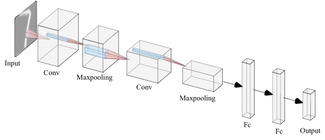
Figure 1: An overview of LeNet network r45_5265772 . This is a small neural network which only includes two convolution layers but make great achievement on some small dataset such as MNIST r42_deng2012mnist and FASHION MNIST r44_xiao2017/online .

3.2 Standard trainig and adversarial training

Standard Training

Given a training set with $N$ samples $D=\{(\boldsymbol{x}^{(i)},y^{(i)})\}^{N}_{i=1}$, we can learn a classifier $f:X\rightarrow Y$, where $\hat{y}=\mathop{\arg\max}_{i}f_{i}(\boldsymbol{x})$ represents the prediction result of the classifier on the sample $(\boldsymbol{x},y)\in\{(\boldsymbol{x}^{(i)},y^{(i)})\}^{N}_{i=1}$. Then, the training process can be described as the following optimization problem:

$$\min\mathop{E}_{(\boldsymbol{x},y)\backsim D}[L(f(\boldsymbol{x}),y)]=\min\sum_{i=1}^{N}L(f(\boldsymbol{x}^{(i)}),y^{(i)}),$$ (2)

where $L$ represents the loss function.

Adversarial Training

The set of adversarial examples concerning a sample $(\boldsymbol{x},y)$ is defined as

$$\begin{split}B_{l}(\boldsymbol{x},y,f)=\{\boldsymbol{x}_{adv}|\|\boldsymbol{x}_{adv}-\boldsymbol{x}\|_{l}\leq\epsilon,\\ \arg\max_{j}f_{j}(\boldsymbol{x}_{adv})\neq y\},\end{split}$$ (3)

where $l$ represents $l$-norm. Then, the process of its adversarial training can be formulated as follows:

$$\min\mathop{E}_{(\boldsymbol{x},y)\backsim D}[\max_{\boldsymbol{x}_{adv}\in B_{l}}L(f(\boldsymbol{x}_{adv}),y)].$$ (4)

There are some differences between standard training and adversarial training as follows.

• Adversarial training needs more samples than standard training. To improve the adversarial robustness of the model and make effective defense to both known and unknown attacks, the adversarial examples generated by powerful attacks would be added to the training dataset. The DNNs will learn more knowledge from adversarial examples than standard training.

• Adversarial training is more time-consuming than standard training. It is obvious that the adversarial examples are generated during the training process. The more complicated the generating algorithm, and the more iterations it includes, the longer time it will consume.

• Some works r20_kurakin2018ensemble ; r26_athalye2018obfuscated ; r47_qin2019adversarial show that adversarial training may cause a phenomenon, called obfuscated gradients, which will give a false sense of security in defenses against adversarial examples. A good model should be able to make effective defense to adversarial examples, at the same time avoid obfuscated gradients.

• Adversarial training may decrease the accuracy of the model on a clean dataset. Tsipras et al. r51_tsipras2018robustness point out that robustness may be conflicting with accuracy, causing the so-called accuracy-robustness problem. Empirically, many works r35_zhang2019theoretically ; r49_su2018robustness ; r50_kurakin2016adversarial ; r9_wong2017provable ; r38_raghunathan2018certified show that adversarial training is to achieve a trade-off between adversarial robustness and accuracy.

3.3 Empirical observation

In order to analyse the difference between the standard model and the adversarial model, we make an investigation on the parameters of the convolutional layer.

By using LeNet, we conduct two experiments for both standard training and adversarial training on MNIST dataset. The detailed setting such as learning rate, epochs and batchsize are listed in Section 5. It is noteworthy that, during adversarial training, the model updates parameters alternately between clean samples and adversarial samples.

Fig. 2 shows the distribution and the parameter values of the first convolutional layer in LeNet. It can be seen that after adversarial training, most parameters of the first convolutional layer become smaller, only a small part of them remain unchanged or become larger. By investigations on more data sets, we claim that this phenomenon is not accidential. It commonly exists in the first convolutional layer of LeNet, and sometimes can be found in the second convolutional layer.

Based on above discovery, we give the following proposition to explore more significant property in neural network.

Proposition 1

Given a neural network model, if most parameters in the convolutional layer approach zero, while only a small part of parameters are far away from zero, then the model have a good adversarial robustness. This property is called Min-Max property.

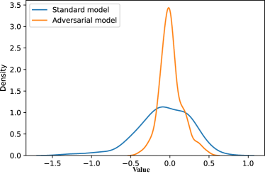
(a)

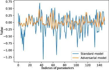
(b)

Figure 2: Standard training and adversarial training: (a) The distribution of parameter of the first convolutional layer in LeNet. (b) The values of parameters of the first convolutional layer in LeNet network (Sort from left to right, top to bottom).

3.4 Min-Max property

The robustness of a DNN model against adversarial examples can be improved by adversarial training, which is well acknowledged in the machine learning and image processing communities. It is observed that in LeNet structure, the absolute values of most weights in convolutional layers will become very small (approaching zero) or very large (depending on the specific weights) after several rounds of adversarial training. We call this phenomenon Min-Max property.

It is noteworthy that a deep model with strong robustness against adversarial examples may not have the Min-Max property. However, based on a considerable number of simulations, it is observed that a deep model with the Min-Max property usually has strong robustness against adversarial examples. More importantly, the Min-Max property can be achieved without adversarial training. Thus, a well-trained deep model with the Min-Max property will possibly have strong robustness and adversarial training is no longer needed. Motivated by these observations, we propose a new training scheme as below based on Eq. 2.

$$\min\mathop{E}_{(\boldsymbol{x},y)\backsim D}[L(f(\boldsymbol{x}),y)+\lambda\|W_{conv}\|_{1}-\mu\|W_{conv}\|^{2}_{2}],$$ (5)

where $\lambda$ and $\mu$ are hyperparamters, and $W_{conv}$ is the parameter of convolution. The term $\|W_{conv}\|_{1}$ makes the parameters approach zero, and while the term $\|W_{conv}\|^{2}_{2}$ makes the parameters be far away from zero.

In comparison with the original training scheme of Eq. 4, Eq. 5 no longer needs adversarial training but still can improve the adversarial robustness of the model. In practice, we use the combination of $\lambda\|W_{conv}\|_{1}$ and $-\mu\|W_{conv}\|^{2}_{2}$ to control the Min-Max property of the model.

In the following, we try to mathematically explain why the Min-Max property is able to lead to strong robustness against adversarial examples via a simplified convolutional neural network. Essentially, convolutional operation is a linear transformation of feature space. For simplication, in some cases, a ReLU operation is required after convolution, which makes the result piecewise linear. It is noteworthy that some scholars consider the convolution with ReLU as a non-linear transformation in functionality but actually, it is piecewise linear. Based on these analysis, we propose two simplified models as follows.

Considering a single network $f(\boldsymbol{x})=\boldsymbol{W}\boldsymbol{x}$ where $\boldsymbol{W}$ is a $m\times n$ matrix, $\boldsymbol{x}$ is a $n\times 1$ vector, $m$ is the number of training samples and $n$ is the number of features. By adopting cross entropy loss, the loss function of this network is represented as $L(\boldsymbol{x};\boldsymbol{W})=-\boldsymbol{y}^{T}log(softmax(\boldsymbol{W}\boldsymbol{x}))$ where $\boldsymbol{y}$ is a one-hot vector, and

$$softmax(\boldsymbol{a})=exp(\boldsymbol{a})/(\boldsymbol{1}^{T}exp(\boldsymbol{a})).$$

The two models are given as follows:

• $Model\#1$: $L_{a}(\boldsymbol{x};\boldsymbol{W_{a}})=-\boldsymbol{y}^{T}log(softmax(\boldsymbol{W_{a}}\boldsymbol{x}))$, where $W_{a}=(a_{ij})$ and $a_{ij}\sim U(0,1)$.

• $Model\#2$: $L_{b}(\boldsymbol{x};\boldsymbol{W_{b}})=-\boldsymbol{y}^{T}log(softmax(\boldsymbol{W_{b}}\boldsymbol{x}))$, where $W_{b}=(b_{ij})$ and $b_{ij}\sim B(1,p_{1})$, $B(1,p_{1})$ is the binomial distribution, and $p_{1}$ represents the probability of $b_{ij}=1$ where $p_{1}>0,p_{1}<<1$.

Suppose $a_{ij}$ follows a uniform distribution in [0, 1], and $b_{ij}$ follows a binomial distribution $B(1,p_{1})$ where $p_{1}<<1$ for each $i$ and $j$. We have the following theorem:

Theorem 1

Suppose $\boldsymbol{x}$ is a vector and $\boldsymbol{x}_{i}$ is the $i$th element in $\boldsymbol{x}$, $\forall i$, the following inequality holds

$$\lvert\frac{\partial\mathbb{E}_{b_{ij}\sim B(1,p_{1})}L_{b}(\boldsymbol{x};\boldsymbol{W_{b}})}{\partial\boldsymbol{x}_{i}}\rvert\leq\lvert\frac{\partial\mathbb{E}_{a_{ij}\sim U(0,1)}L_{a}(\boldsymbol{x};\boldsymbol{W_{a}})}{\partial\boldsymbol{x}_{i}}\rvert.$$

From Theorem 1 we know that the following inequality approximately holds:

$$\begin{split}\|L_{b}(\boldsymbol{x};\boldsymbol{W_{b}})-L_{b}(\boldsymbol{x+\Delta};\boldsymbol{W_{b}})\|\leq\|L_{a}(\boldsymbol{x};\boldsymbol{W_{a}})-\\ L_{a}(\boldsymbol{x+\Delta};\boldsymbol{W_{a}})\|,\end{split}$$

where $\boldsymbol{\Delta}$ is a small perturbation of the observation $\boldsymbol{x}$. It shows that the perturbation of input to $Model\#1$ is more sensitive than that to $Model\#2$, which indicates that, to a great extent, the attacker can find the adversarial examples in the neighbourhood of clean samples for $Model\#1$ more easily than for $Model\#2$.

Proof

Firstly, we compute the partial derivative $\frac{\partial L(\boldsymbol{x};\boldsymbol{W})}{\partial\boldsymbol{x}}$ where $L(\boldsymbol{x};\boldsymbol{W})=-\boldsymbol{y}^{T}log(softmax(\boldsymbol{W}\boldsymbol{x}))$. We mark $\boldsymbol{a}=\boldsymbol{W}\boldsymbol{x}$ where $\boldsymbol{W}$ is a $m\times n$ matrix and $\boldsymbol{x}$ is a $n\times 1$ vector. Let $\sigma(\boldsymbol{a})=softmax(\boldsymbol{a})$.

Then, $L(\boldsymbol{x};\boldsymbol{W})$ can be rewritten in a scalar form:

$$\begin{split}L(\boldsymbol{x};\boldsymbol{W})&=-\boldsymbol{y}^{T}log(softmax(\boldsymbol{W}\boldsymbol{x}))\\ &=-\boldsymbol{y}^{T}log\ \sigma(\boldsymbol{a})\\ &=-\sum_{j=1}^{m}y_{j}log\ \sigma_{j}(\boldsymbol{a}),\end{split}$$

where $\sigma_{j}(\boldsymbol{a})=\frac{\exp(a_{j})}{\sum_{t=1}^{m}\exp(a_{t})}$ and $a_{j}=\sum_{i=1}^{n}w_{ji}x_{i}$.

We have

$$\begin{split}\frac{\partial a_{j}}{\partial x_{i}}&=\frac{\partial}{\partial x_{i}}\sum_{k=1}^{m}w_{jk}x_{k}\\ &=w_{ji}\end{split}$$

and

$$\frac{\partial\sigma_{i}(\boldsymbol{a})}{\partial a_{j}}=\left\{\begin{aligned} \sigma_{i}(1-\sigma_{j})&&{i=j}\\ -\sigma_{i}\sigma_{j}&&{i\neq j}.\end{aligned}\right.$$

Applying the chain rule, we have

$$\begin{split}\frac{\partial L}{\partial a_{j}}&=\sum_{i}\frac{\partial L}{\partial\sigma_{i}}\cdot\frac{\partial\sigma_{i}}{\partial a_{j}}=\frac{\partial L}{\partial\sigma_{j}}\cdot\frac{\partial\sigma_{j}}{\partial a_{j}}+\sum_{i\neq j}\frac{\partial L}{\partial\sigma_{i}}\cdot\frac{\partial\sigma_{i}}{\partial a_{j}}\\ &=-y_{j}\frac{1}{\sigma_{j}}\cdot\sigma_{j}(1-\sigma_{j})+\sum_{i\neq j}\frac{-y_{i}}{\sigma_{i}}\cdot(-1)\sigma_{j}\sigma_{i}\\ &=-y_{j}(1-\sigma_{j})+\sum_{i\neq j}y_{i}\sigma_{j}\\ &=-y_{j}+y_{j}\sigma_{j}+\sum_{i\neq j}y_{i}\sigma_{j}\\ &=\sigma_{j}-y_{j}.\end{split}$$

As a result we have

$$\begin{split}\frac{\partial L}{\partial x_{i}}&=\sum_{j=1}^{m}\frac{\partial L}{\partial a_{j}}\cdot\frac{\partial a_{j}}{\partial x_{i}}\\ &=\sum_{j=1}^{m}w_{ji}\frac{\partial L}{\partial a_{j}}\\ &=\sum_{j=1}^{m}w_{ji}(\sigma_{j}-y_{j}).\end{split}$$ (6)

We can rewrite Eq. 6 in matrix form:

$$\frac{\partial L(\boldsymbol{x};\boldsymbol{W})}{\partial\boldsymbol{x}}=\boldsymbol{W}^{T}(-\boldsymbol{y}+\sigma(\boldsymbol{W}\boldsymbol{x})).$$

Then

$$\begin{split}&\lvert\frac{\partial\mathbb{E}_{a_{ij}\sim U(0,1)}[L_{a}(\boldsymbol{x};\boldsymbol{W_{a}})]}{\partial x_{i}}\rvert\\ &=\lvert\mathbb{E}_{a_{ij}\sim U(0,1)}[\frac{\partial L_{a}(\boldsymbol{x};\boldsymbol{W_{a}})}{\partial x_{i}}]\rvert\\ &=\lvert\mathbb{E}_{a_{ij}\sim U(0,1)}[\sum_{j=1}^{m}w_{ji}(\sigma_{j}-y_{j})]\rvert\\ &=\lvert\sum_{j=1}^{m}\frac{1}{2}(\sigma_{j}-y_{j})\rvert\\ &=\frac{1}{2}(1-\sum_{j=1}^{m}\sigma_{j}).\end{split}$$

In a similar way, we obtain

$$\begin{split}&\lvert\frac{\partial\mathbb{E}_{b_{ij}\sim B(1,p_{1})}[L_{b}(\boldsymbol{x};\boldsymbol{W_{b}})]}{\partial\boldsymbol{x_{i}}}\rvert=p_{1}(1-\sum_{j=1}^{m}\sigma_{j}).\end{split}$$

Since $p_{1}>0$ and $p_{1}\ll(1-p_{1})$, then $p_{1}<\frac{1}{2}$. Therefore,

$$p_{1}(1-\sum_{j=1}^{m}\sigma_{j})\leq\frac{1}{2}(1-\sum_{j=1}^{m}\sigma_{j})$$

Thus,

$$\lvert\frac{\partial\mathbb{E}_{b_{ij}\sim B(1,p_{1})}L_{b}(\boldsymbol{x};\boldsymbol{W_{b}})}{\partial\boldsymbol{x}_{i}}\rvert\\ \leq\lvert\frac{\partial\mathbb{E}_{a_{ij}\sim U(0,1)}[L_{a}(\boldsymbol{x};\boldsymbol{W_{a}})]}{\partial\boldsymbol{x}_{i}}\rvert$$

If $p_{1}=\frac{1}{2}$ then the equality holds. Thus, Theorem 1 is proven. $\hfill\blacksquare$

4 Uncertainty in Min-Max property

In this section, we try to explain the Min-Max property from the perspective of uncertainty. It has been proved that uncertainty is inevitable when making decision for a sample r57_yeung2002improving . This uncertainty is usually caused by the fuzziness of the similarity matrix.

In the proposed training scheme, i.e., Eq. 5, the minimization of $(\|W_{conv}\|_{1}-\|W_{conv}\|^{2}_{2})$ makes the parameters have the Min-Max property. For the convenience of computing, let

$$M(W_{conv})=\|W_{conv}\|_{1}-\|W_{conv}\|_{2}^{2},$$ (7)

where we consider $W_{conv}$ as a vector denoted by

$$W_{conv}=[w_{1},w_{2},...,w_{n}]^{T}.$$ (8)

In view of the changing tendency of $w_{i}\ (1\leq i\leq n)$, minimizing Eq. 7 equals to minimizing $M(W_{conv})$.

Then we have

$$\begin{split}M(W_{conv})&=\|W_{conv}\|_{1}-\|W_{conv}\|_{2}^{2}\\ &=\sum_{i=1}^{n}|w_{i}|-\sum_{1}^{n}|w_{i}|^{2}\\ &=\sum_{i=1}^{n}|w_{i}|(1-|w_{i}|).\end{split}$$ (9)

Eq. 9 is derived from a simple function, i.e.,

$$f(x)=|x|(1-|x|),x\in R.$$ (10)

From this function, we have

$$f^{\prime}(x)=\left\{\begin{aligned} 1-2x&,&{x\geq 0}\\ -1-2x&,&{x<0}.\end{aligned}\right.$$ (11)

Thus,

$$\left\{\begin{aligned} f^{\prime}(x)\geq 0&,&{x\leq-\frac{1}{2}\cup 0\leq x\leq\frac{1}{2}}\\ f^{\prime}(x)<0&,&{-\frac{1}{2}<x<0\cup x>\frac{1}{2}}.\end{aligned}\right.$$ (12)

Therefore, from Eq. 7, we know that $M$ with respect to $w_{i}$ is a strictly monotonically increasing function under the condition of $x\leq-\frac{1}{2}\cup 0\leq x\leq\frac{1}{2}$ and is a strictly monotonically decreasing function under the condition of $-\frac{1}{2}<x<0\cup x>\frac{1}{2}$. By minimizing Eq. 7, the positive values in the parameters will be far away from $0.5$ and the negative values in the parameters will be far away from $-0.5$. Based on this statement, we have the following equality

$$\begin{split}\min M(W_{conv})=\lim\limits_{w_{i}\rightarrow 0\ \text{or}\ w_{i}\rightarrow\infty}M(W_{conv}).\end{split}$$ (13)

According to r58_basak1998unsupervised , the fuzziness of this vector can be define as

$$\begin{split}Fuzziness(W_{conv})=-\frac{1}{N}\sum_{1}^{N}[\rho_{i}log\rho_{i}+\\ (1-\rho_{i})log(1-\rho_{i})],\end{split}$$ (14)

where $N$ is the size of vector $W_{conv}$ and $\rho_{i}$ is defined as follows:

$$\rho_{i}=\frac{1}{1+|w_{i}|}.$$ (15)

From Eq. 15, we have

$$w_{i}\rightarrow 0\Rightarrow\rho_{i}\rightarrow 1,$$

$$w_{i}\rightarrow\infty\Rightarrow\rho_{i}\rightarrow 0.$$

These two cases (e.g. $\rho_{i}\rightarrow 1$ and $\rho_{i}\rightarrow 0$) are far away from $0.5$ which is the extreme value of Eq. 14. Therefore, the fuzziness of the parameters will decrease as minmizing the $M(W_{conv})$.

5 Experiments and results

In this section, we evaluate the adversarial robustness of the proposed model on MNIST r42_deng2012mnist dataset and CIFAR10 r43_krizhevsky2009learning dataset by adopting LeNet as the network structure. The adversarial robustness of the model is measured by the accuracy under adversarial attacks. Besides, we also calculate the fuzziness of parameters in convolutional layer to evaluate the uncertainty of the model.

5.1 Experimental setup

The experiments are conducted under Python 3.6 with the Advertorch toolbox r56_ding2019advertorch . Before training, the input values are normalized by $(x-\mu)/\sigma$, where $\mu$ and $\sigma$ are the mean and variance among all samples. For MNIST, we have $\mu=0.1307$ and $\sigma=0.3081$; while for CIFAR10, we have $\mu=(0.4914,0.4822,0.4465)$ and $\sigma=(0.2023,0.1994,0.2010)$.

We compare the performance of four models without adversarial training:

• Standard model (Std.): This is a model trained with clean examples by adopting cross-entropy as the loss function.

• Standard model with L1 normalization (Std.+L1): This is a model trained with clean examples, and the loss function includes an additional L1 normalization related to parameters.

• Standard model with L2 normalization (Std.+L2): This is a model trained with clean examples, and the loss function includes and additional L2 normalization related to parameters.

• Min-Max model (Min-Max): This is a model trained with clean examples and our proposed objective function 5.

Std.+L1 and Std.+L2 are designed for ablation study since the proposed objective function is composed of L1 normalization and L2 normalization. Moreover, these models have the same framework and setting.

As for the datasets, we briefly introduce them as follows:

• MNIST dataset consists of 60,000 training samples and 10,000 testing samples, each of which is a 28x28 pixel handwriting digital image. By setting $batchsize=64,lr=0.001,epochs=10$, we use Adam optimization to train the neural network. When evaluating the model with Advertorch, we adopt some attacks (FGSM r23_goodfellow2014explaining , PGD r22_madry2017towards , CW r24_carlini2017towards , MIA r68_dong2018boosting , L2BIA r50_kurakin2016adversarial and LinfBIA r50_kurakin2016adversarial ) widely used where $epsilon=0.3$.

• CIFAR10 dataset is composed of 60,000 32x32 colour image, 50,000 for training and 10,000 for testing. By setting $batchsize=64,lr=0.01,epochs=90$, we use Adam optimization to train the neural network where the learning rate halved every 30 epochs. When evaluating the adversarial robustness, we set $epsilon=0.03$.

5.2 Adversarial robustness

We use six attack methods to evaluate the adversarial robustness of the model, i.e., FGSM r23_goodfellow2014explaining , PGD r22_madry2017towards , CW r24_carlini2017towards , MIA r68_dong2018boosting , L2BIA r50_kurakin2016adversarial and LinfBIA r50_kurakin2016adversarial . The higher accuracy under adversarial attack, the stronger adversarial robustness of the model. We set $epsilon=0.3$ for MNIST dataset and set $epsilon=0.03$ for CIFAR10 dataset.

Table 1 shows the adversarial robustness of the standard model and Min-Max model regarding the testing accuracy under various adversarial attacks. It can be seen that the proposed the Min-Max model has stronger adversarial robustness than the standard model under all of the attack methods. This result experimentally verifies the correctness of Theorem 1, i.e., the model will have the Min-Max property by minimizing Eq. 5, and this property makes it have stronger adversarial robustness. Moreover, Fig. 3 shows the training loss of the standard model and Min-Max model. It can be observed that the Min-Max model converges slower than the standard model but is more stable after convergence.

Table 1: MNIST: The comparison of accuracy between standard models (Std., Std.+L1 and Std.+L2) and Min-Max model.

	Std.	Std.+L1	Std.+L2	Min-Max
No attack	0.9861	0.9747	0.9576	0.9844
FGSM	0.8152	0.7610	0.7631	0.9475
PGD	0.5928	0.6198	0.7130	0.8369
CW	0.5697	0.4961	0.5403	0.6892
MIA	0.6268	0.6190	0.7181	0.6980
L2BIA	0.9747	0.9659	0.9501	0.9765
LinfBIA	0.6046	0.6276	0.7126	0.8599

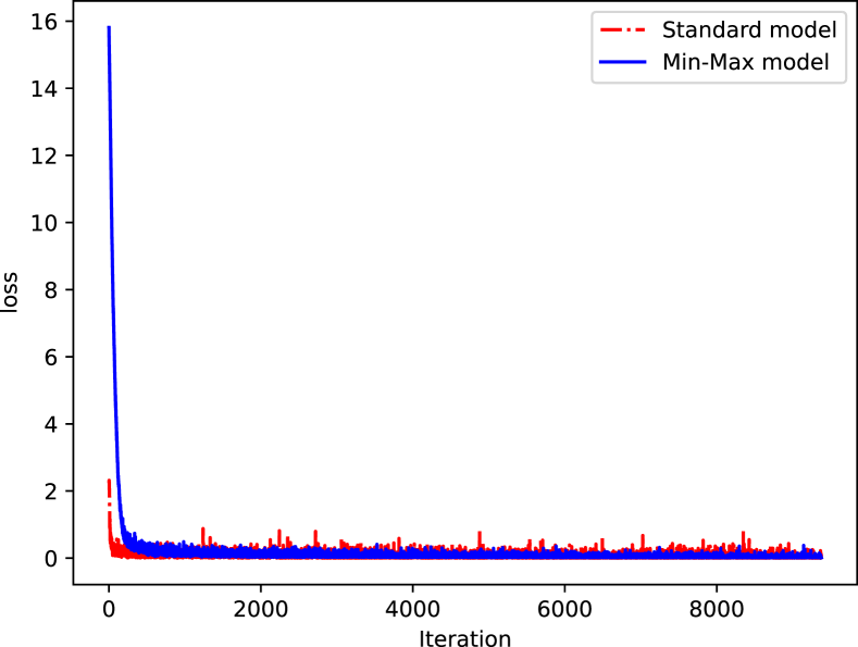
Figure 3: MNIST: The comparison of training loss between standard training and adversarial training. After convergence, Min-Max model is more stable than standard model.

Table 2 further reports the comparison results between the standard model and the Min-Max model on a more complicated dataset, i.e., CIFAR10. It can be seen that the Min-Max property significantly improves the adversarial robustness of the model, which is consistent with the conclusion on MNIST dataset. However, this improvement is limited. For some powerful adversarial attacks such as CW, the model is still vulnerable. This may be due to the fact that CW is a non-gradient adversarial attack. Min-Max property in the convolutional layer can avoid sharp change by small perturbation which is spread by the gradient in the neural network. However, if the small perturbation is not dependent on the gradient, it will be difficult for the Min-Max property to catch the exception.

It is noteworthy that the proposed objective function, i.e., Eq. 5, contains both L1 normalization and L2 normalization. In order to investigate the effectiveness of these two normalizations, we ablate one of them. As shown in Tables 1 and 2, L1 normalization does not help to improve the adversarial robustness and L2 normalization can improve the adversarial robustness a little bit. However, by combining L1 normalization and L2 normalization, the Min-Max model has much stronger adversarial robustness than both Std.+L1 and Std.+L2 under most attacks. This shows that Eq. 5 can effectively make the parameters either closer to zero or further away from zero, as described in the Min-Max property.

Table 2: CIFAR10: The comparison of accuracy between standard models (Std., Std.+L1 and Std.+L2) and Min-Max model.

	Std.	Std.+L1	Std.+L2	Min-Max
No attack	0.6352	0.5589	0.6573	0.5668
FGSM	0.2382	0.3144	0.3716	0.3927
PGD	0.1669	0.2937	0.3416	0.3712
CW	0.0000	0.0000	0.0000	0.0000
MIA	0.1583	0.2918	0.3382	0.3633
L2BIA	0.6249	0.5550	0.5561	0.6512
LinfBIA	0.2128	0.3135	0.3594	0.3860

5.3 Uncertainty

We make an investigation on the fuzziness of parameters in the first convolutional layer of LeNet using Eq. 14. The standard model, the adversarial model and the Min-Max model are compared. It is noteworthy that the adversarial model is trained alternately between clean examples and adversarial examples in each epoch, where the adversarial examples are generated by PGD r22_madry2017towards . With this training scheme, the phenomenon of accuracy-robustness problem would reduce.

Figs. 4 and 5 show the distribution of parameters in the first convolutional layer of LeNet for dataset MNIST and CIFAR10, respectively. It can be seen that for both of these two datasets, the number of parameters close to zero in the adversarial model is larger than that in the standard model. This is the basis for the proposed Min-Max property. Then, by further using Eq. 5, this property in the Min-Max model becomes more obvious. The intuitive result is shown in Figs. 4 and 5. The number of parameters close to zero in the Min-Max model is about 17-19 times of that in the standard model for MNIST, and is about 140-150 times for CIFAR10. We suspect that this extreme phenomenon is responsible for the decline in the accuracy on clean examples, as a result, the accuracy of the Min-Max model on clean examples is lower than that of the standard model.

Moreover, we utilize fuzziness (Eq. 14) to quantify the Min-Max property. As shown in Table 3, the fuzziness of the adversarial model is lower than that of the standard model, demonstrating a lower uncertainty of the adversarial model. By minimizing Eq. 5, the uncertainty of the Min-Max model is further reduced.

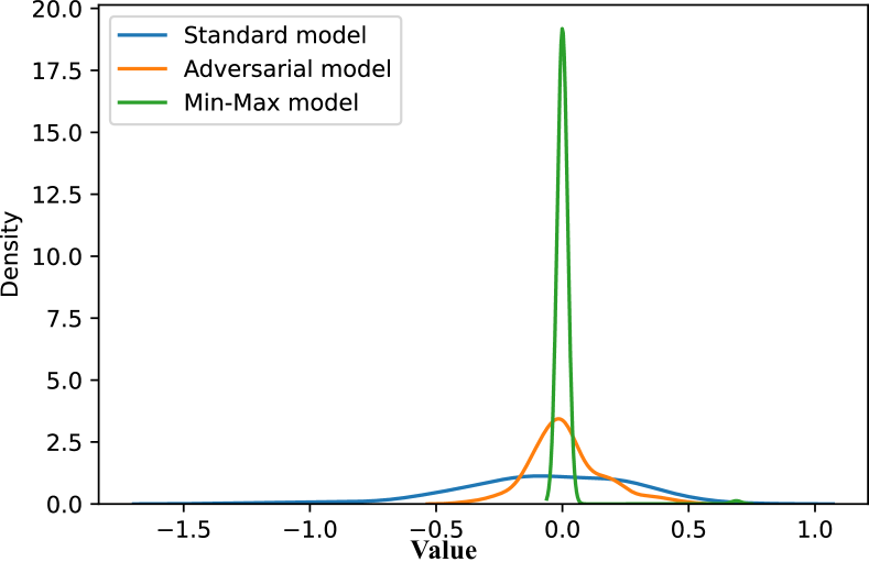
Figure 4: MNIST: The comparison of parameter distribution in the first convolutional layer of LeNet among standard model, adversarial model and Min-Max model.

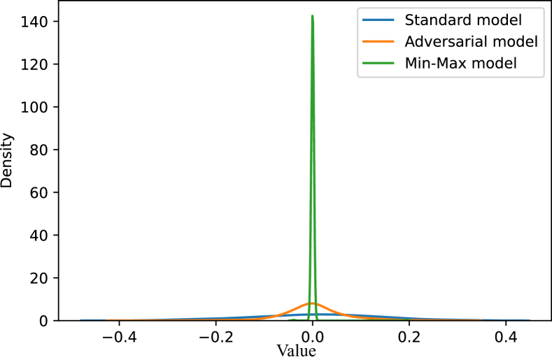
Figure 5: CIFAR10: The comparison of parameter distribution in first convolutional layer of LeNet among standard model, adversarial model and Min-Max model.

Table 3: The fuzziness of parameters of fist convolutional layer in LeNet.

	MNIST	CIFAR10
Standard model	0.4417	0.2842
Adv. model	0.2611	0.1594
Min-Max model	0.0053	0.0016

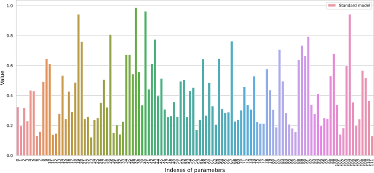
(a)

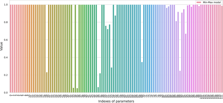
(b)

Figure 6: The part of normalized parameters in first convolutional layer in the task of CIFAR10: (a) The normalized parameters in standard model. (b) The normalized parameters in Min-Max model.

5.4 Disscussion

It is investigated that Min-Max property would cause a drop in accuracy on clean examples. This phenomenon is not obvious on MNIST but is easily aware on CIFAR10. As shown in Table 2, accuracy of the Min-Max model on clean examples drops about 0.089 compared with the standard model. This phenomenon brings the so-called accuracy-robustness problem. Although the trade-off between accuracy and robustness is widely discussed r51_tsipras2018robustness ; r35_zhang2019theoretically ; r49_su2018robustness ; r50_kurakin2016adversarial ; r9_wong2017provable ; r38_raghunathan2018certified , the underlying theories still remain unknown. Through observing the quantitative indicator of the uncertainty, e.g., fuzziness, we find that the uncertainty of the Min-Max model has dropped to be too low as shown in Table 3. Similar observations can also be made from Figs. 4 and 5. Therefore, we guess that the accuracy-robustness problem is caused by this extreme phenomenon of the Min-Max property to some extent.

Finally, we observe the normalized convolutional vector in both standard training and our training strategies. We show part of parameters in the first convolutional layer for the task of CIFAR10, where the values are ranked according to their indexes of position. By Eq. 15, we normalize the values into a fixed range ([0, 1]). As shown in Fig. 6, it is easy to see that the numbers approach zero or one in the Min-Max model are much larger than that of the standard model. It intuitively shows that the uncertainty of our training strategies is far lower than that of the standard model.

6 Conclusion

The Min-Max property is extracted by observing the difference between the standard model and the adversarial model in the convolutional layer. This Min-Max property is a phenomenon that the parameters in the convolutional layer will be either closer to zero or farther away from zero. Possessing the Min-Max property of the model have stronger adversarial robustness. According to this property, we design a new objective function. And minimizing this objective function equals making the model with the Min-Max property. We theoretically and experimentally validate the correctness of the Min-Max property. Moreover, from the perspective of uncertainty, we use fuzziness to quantify the Min-Max property. As a result, the process of maximizing the Min-Max property is equivalent to minimizing the fuzziness of parameters. In future works, we will explore the Min-Max property in a more complicated DNN structure and try to discover properties of uncertainty in DNN. Moreover, how to further improve the adversarial robustness based on uncertainty analysis is also worth to study in the future.

Conflict of interest

The authors declare that there is no conflict of interests regarding the publication of this article.

References

- (1) Abbasi, M., Gagné, C.: Robustness to adversarial examples through an ensemble of specialists. In: 5th International Conference on Learning Representations, ICLR 2017, Toulon, France, April 24-26, 2017, Workshop Track Proceedings. OpenReview.net (2017). URL https://openreview.net/forum?id=S1cYxlSFx
- (2) Athalye, A., Carlini, N., Wagner, D.A.: Obfuscated gradients give a false sense of security: Circumventing defenses to adversarial examples. In: J.G. Dy, A. Krause (eds.) Proceedings of the 35th International Conference on Machine Learning, ICML 2018, Stockholmsmässan, Stockholm, Sweden, July 10-15, 2018, Proceedings of Machine Learning Research, vol. 80, pp. 274–283. PMLR (2018). URL http://proceedings.mlr.press/v80/athalye18a.html
- (3) Basak, J., De, R.K., Pal, S.K.: Unsupervised feature selection using a neuro-fuzzy approach. Pattern Recognition Letters 19(11), 997–1006 (1998)
- (4) Bradshaw, J., Matthews, A.G.d.G., Ghahramani, Z.: Adversarial examples, uncertainty, and transfer testing robustness in gaussian process hybrid deep networks. arXiv preprint arXiv:1707.02476 (2017)
- (5) Brown, T.B., Mané, D., Roy, A., Abadi, M., Gilmer, J.: Adversarial patch. arXiv preprint arXiv:1712.09665 (2017)
- (6) Carlini, N., Wagner, D.: Towards evaluating the robustness of neural networks. In: 2017 ieee symposium on security and privacy (sp), pp. 39–57. IEEE (2017)
- (7) Chen, H.Y., Liang, J.H., Chang, S.C., Pan, J.Y., Chen, Y.T., Wei, W., Juan, D.C.: Improving adversarial robustness via guided complement entropy. In: Proceedings of the IEEE International Conference on Computer Vision, pp. 4881–4889 (2019)
- (8) Chen, H.Y., Liang, J.H., Chang, S.C., Pan, J.Y., Chen, Y.T., Wei, W., Juan, D.C.: Improving adversarial robustness via guided complement entropy. In: Proceedings of the IEEE International Conference on Computer Vision, pp. 4881–4889 (2019)
- (9) Chen, P.Y., Zhang, H., Sharma, Y., Yi, J., Hsieh, C.J.: Zoo: Zeroth order optimization based black-box attacks to deep neural networks without training substitute models. In: Proceedings of the 10th ACM Workshop on Artificial Intelligence and Security, pp. 15–26 (2017)
- (10) Clevert, D., Unterthiner, T., Hochreiter, S.: Fast and accurate deep network learning by exponential linear units (elus). In: Y. Bengio, Y. LeCun (eds.) 4th International Conference on Learning Representations, ICLR 2016, San Juan, Puerto Rico, May 2-4, 2016, Conference Track Proceedings (2016). URL http://arxiv.org/abs/1511.07289
- (11) Deng, L.: The mnist database of handwritten digit images for machine learning research [best of the web]. IEEE Signal Processing Magazine 29(6), 141–142 (2012)
- (12) Ding, G.W., Wang, L., Jin, X.: AdverTorch v0.1: An adversarial robustness toolbox based on pytorch. arXiv preprint arXiv:1902.07623 (2019)
- (13) Dong, Y., Liao, F., Pang, T., Su, H., Zhu, J., Hu, X., Li, J.: Boosting adversarial attacks with momentum. In: Proceedings of the IEEE conference on computer vision and pattern recognition, pp. 9185–9193 (2018)
- (14) Eykholt, K., Evtimov, I., Fernandes, E., Li, B., Rahmati, A., Xiao, C., Prakash, A., Kohno, T., Song, D.: Robust physical-world attacks on deep learning visual classification. In: Proceedings of the IEEE Conference on Computer Vision and Pattern Recognition, pp. 1625–1634 (2018)
- (15) Glorot, X., Bordes, A., Bengio, Y.: Deep sparse rectifier neural networks. In: Proceedings of the fourteenth international conference on artificial intelligence and statistics, pp. 315–323 (2011)
- (16) Goodfellow, I.J., Shlens, J., Szegedy, C.: Explaining and harnessing adversarial examples. In: Y. Bengio, Y. LeCun (eds.) 3rd International Conference on Learning Representations, ICLR 2015, San Diego, CA, USA, May 7-9, 2015, Conference Track Proceedings (2015). URL http://arxiv.org/abs/1412.6572
- (17) Haykin, S., Kosko, B.: GradientBased Learning Applied to Document Recognition, pp. 306–351 (2001)
- (18) Hein, M., Andriushchenko, M.: Formal guarantees on the robustness of a classifier against adversarial manipulation. In: Advances in Neural Information Processing Systems, pp. 2266–2276 (2017)
- (19) Karmon, D., Zoran, D., Goldberg, Y.: Lavan: Localized and visible adversarial noise. In: J.G. Dy, A. Krause (eds.) Proceedings of the 35th International Conference on Machine Learning, ICML 2018, Stockholmsmässan, Stockholm, Sweden, July 10-15, 2018, Proceedings of Machine Learning Research, vol. 80, pp. 2512–2520. PMLR (2018). URL http://proceedings.mlr.press/v80/karmon18a.html
- (20) Krippendorff, K.: Figure 12 in klaus krippendorff’s ’ross ashby’s information theory: a bit of history, some solutions to problems, and what we face today’, International Journal of General Systems, 38, 189-212, 2009. Int. J. Gen. Syst. 38(6), 667–668 (2009). DOI 10.1080/03081070902993178. URL https://doi.org/10.1080/03081070902993178
- (21) Krizhevsky, A., Hinton, G., et al.: Learning multiple layers of features from tiny images (2009)
- (22) Kurakin, A., Goodfellow, I.J., Bengio, S.: Adversarial examples in the physical world. In: 5th International Conference on Learning Representations, ICLR 2017, Toulon, France, April 24-26, 2017, Workshop Track Proceedings. OpenReview.net (2017). URL https://openreview.net/forum?id=HJGU3Rodl
- (23) Kurakin, A., Goodfellow, I.J., Bengio, S.: Adversarial machine learning at scale. In: 5th International Conference on Learning Representations, ICLR 2017, Toulon, France, April 24-26, 2017, Conference Track Proceedings. OpenReview.net (2017). URL https://openreview.net/forum?id=BJm4T4Kgx
- (24) Lin, J.: Divergence measures based on the shannon entropy. IEEE Transactions on Information theory 37(1), 145–151 (1991)
- (25) Liu, H., Ji, R., Li, J., Zhang, B., Gao, Y., Wu, Y., Huang, F.: Universal adversarial perturbation via prior driven uncertainty approximation. In: Proceedings of the IEEE/CVF International Conference on Computer Vision (ICCV) (2019)
- (26) Liu, X., Yang, H., Liu, Z., Song, L., Chen, Y., Li, H.: DPATCH: an adversarial patch attack on object detectors. In: H. Espinoza, S.Ó. hÉigeartaigh, X. Huang, J. Hernández-Orallo, M. Castillo-Effen (eds.) Workshop on Artificial Intelligence Safety 2019 co-located with the Thirty-Third AAAI Conference on Artificial Intelligence 2019 (AAAI-19), Honolulu, Hawaii, January 27, 2019, CEUR Workshop Proceedings, vol. 2301. CEUR-WS.org (2019). URL http://ceur-ws.org/Vol-2301/paper_5.pdf
- (27) Liu, Y., Chen, X., Liu, C., Song, D.: Delving into transferable adversarial examples and black-box attacks. In: 5th International Conference on Learning Representations, ICLR 2017, Toulon, France, April 24-26, 2017, Conference Track Proceedings. OpenReview.net (2017). URL https://openreview.net/forum?id=Sys6GJqxl
- (28) Madry, A., Makelov, A., Schmidt, L., Tsipras, D., Vladu, A.: Towards deep learning models resistant to adversarial attacks. In: 6th International Conference on Learning Representations, ICLR 2018, Vancouver, BC, Canada, April 30 - May 3, 2018, Conference Track Proceedings. OpenReview.net (2018). URL https://openreview.net/forum?id=rJzIBfZAb
- (29) Mishkin, D., Matas, J.: All you need is a good init. In: Y. Bengio, Y. LeCun (eds.) 4th International Conference on Learning Representations, ICLR 2016, San Juan, Puerto Rico, May 2-4, 2016, Conference Track Proceedings (2016). URL http://arxiv.org/abs/1511.06422
- (30) Moosavi-Dezfooli, S.M., Fawzi, A., Frossard, P.: Deepfool: a simple and accurate method to fool deep neural networks. In: Proceedings of the IEEE conference on computer vision and pattern recognition, pp. 2574–2582 (2016)
- (31) Papernot, N., McDaniel, P., Goodfellow, I.: Transferability in machine learning: from phenomena to black-box attacks using adversarial samples. arXiv preprint arXiv:1605.07277 (2016)
- (32) Papernot, N., McDaniel, P., Jha, S., Fredrikson, M., Celik, Z.B., Swami, A.: The limitations of deep learning in adversarial settings. In: 2016 IEEE European symposium on security and privacy (EuroS&P), pp. 372–387. IEEE (2016)
- (33) Papernot, N., McDaniel, P., Wu, X., Jha, S., Swami, A.: Distillation as a defense to adversarial perturbations against deep neural networks. In: 2016 IEEE Symposium on Security and Privacy (SP), pp. 582–597. IEEE (2016)
- (34) Pinto, L., Davidson, J., Sukthankar, R., Gupta, A.: Robust adversarial reinforcement learning. In: D. Precup, Y.W. Teh (eds.) Proceedings of the 34th International Conference on Machine Learning, ICML 2017, Sydney, NSW, Australia, 6-11 August 2017, Proceedings of Machine Learning Research, vol. 70, pp. 2817–2826. PMLR (2017). URL http://proceedings.mlr.press/v70/pinto17a.html
- (35) Qin, C., Martens, J., Gowal, S., Krishnan, D., Dvijotham, K., Fawzi, A., De, S., Stanforth, R., Kohli, P.: Adversarial robustness through local linearization. In: Advances in Neural Information Processing Systems, pp. 13847–13856 (2019)
- (36) Raghunathan, A., Steinhardt, J., Liang, P.: Certified defenses against adversarial examples. In: 6th International Conference on Learning Representations, ICLR 2018, Vancouver, BC, Canada, April 30 - May 3, 2018, Conference Track Proceedings. OpenReview.net (2018). URL https://openreview.net/forum?id=Bys4ob-Rb
- (37) Seeger, M.: Gaussian processes for machine learning. International journal of neural systems 14(02), 69–106 (2004)
- (38) Shannon, C.E.: A mathematical theory of communication. ACM SIGMOBILE mobile computing and communications review 5(1), 3–55 (2001)
- (39) Sharif, M., Bhagavatula, S., Bauer, L., Reiter, M.K.: Accessorize to a crime: Real and stealthy attacks on state-of-the-art face recognition. In: Proceedings of the 2016 acm sigsac conference on computer and communications security, pp. 1528–1540 (2016)
- (40) Sinha, A., Namkoong, H., Duchi, J.C.: Certifying some distributional robustness with principled adversarial training. In: 6th International Conference on Learning Representations, ICLR 2018, Vancouver, BC, Canada, April 30 - May 3, 2018, Conference Track Proceedings. OpenReview.net (2018). URL https://openreview.net/forum?id=Hk6kPgZA-
- (41) Smith, L., Gal, Y.: Understanding measures of uncertainty for adversarial example detection. In: A. Globerson, R. Silva (eds.) Proceedings of the Thirty-Fourth Conference on Uncertainty in Artificial Intelligence, UAI 2018, Monterey, California, USA, August 6-10, 2018, pp. 560–569. AUAI Press (2018). URL http://auai.org/uai2018/proceedings/papers/207.pdf
- (42) Springenberg, J.T., Dosovitskiy, A., Brox, T., Riedmiller, M.A.: Striving for simplicity: The all convolutional net. In: Y. Bengio, Y. LeCun (eds.) 3rd International Conference on Learning Representations, ICLR 2015, San Diego, CA, USA, May 7-9, 2015, Workshop Track Proceedings (2015). URL http://arxiv.org/abs/1412.6806
- (43) Su, D., Zhang, H., Chen, H., Yi, J., Chen, P.Y., Gao, Y.: Is robustness the cost of accuracy?–a comprehensive study on the robustness of 18 deep image classification models. In: Proceedings of the European Conference on Computer Vision (ECCV), pp. 631–648 (2018)
- (44) Su, J., Vargas, D.V., Sakurai, K.: One pixel attack for fooling deep neural networks. IEEE Transactions on Evolutionary Computation 23(5), 828–841 (2019)
- (45) Szegedy, C., Vanhoucke, V., Ioffe, S., Shlens, J., Wojna, Z.: Rethinking the inception architecture for computer vision. In: Proceedings of the IEEE conference on computer vision and pattern recognition, pp. 2818–2826 (2016)
- (46) Szegedy, C., Zaremba, W., Sutskever, I., Bruna, J., Erhan, D., Goodfellow, I.J., Fergus, R.: Intriguing properties of neural networks. In: Y. Bengio, Y. LeCun (eds.) 2nd International Conference on Learning Representations, ICLR 2014, Banff, AB, Canada, April 14-16, 2014, Conference Track Proceedings (2014). URL http://arxiv.org/abs/1312.6199
- (47) Terzi, M., Susto, G.A., Chaudhari, P.: Directional adversarial training for cost sensitive deep learning classification applications. Engineering Applications of Artificial Intelligence 91, 103550 (2020)
- (48) Tramèr, F., Kurakin, A., Papernot, N., Goodfellow, I.J., Boneh, D., McDaniel, P.D.: Ensemble adversarial training: Attacks and defenses. In: 6th International Conference on Learning Representations, ICLR 2018, Vancouver, BC, Canada, April 30 - May 3, 2018, Conference Track Proceedings. OpenReview.net (2018). URL https://openreview.net/forum?id=rkZvSe-RZ
- (49) Tsipras, D., Santurkar, S., Engstrom, L., Turner, A., Madry, A.: Robustness may be at odds with accuracy. In: 7th International Conference on Learning Representations, ICLR 2019, New Orleans, LA, USA, May 6-9, 2019. OpenReview.net (2019). URL https://openreview.net/forum?id=SyxAb30cY7
- (50) Wong, E., Kolter, J.Z.: Provable defenses against adversarial examples via the convex outer adversarial polytope. In: J.G. Dy, A. Krause (eds.) Proceedings of the 35th International Conference on Machine Learning, ICML 2018, Stockholmsmässan, Stockholm, Sweden, July 10-15, 2018, Proceedings of Machine Learning Research, vol. 80, pp. 5283–5292. PMLR (2018). URL http://proceedings.mlr.press/v80/wong18a.html
- (51) Xiao, H., Rasul, K., Vollgraf, R.: Fashion-mnist: a novel image dataset for benchmarking machine learning algorithms (2017)
- (52) Yeung, D.S., Wang, X.: Improving performance of similarity-based clustering by feature weight learning. IEEE transactions on pattern analysis and machine intelligence 24(4), 556–561 (2002)
- (53) Zhang, H., Yu, Y., Jiao, J., Xing, E.P., Ghaoui, L.E., Jordan, M.I.: Theoretically principled trade-off between robustness and accuracy. In: K. Chaudhuri, R. Salakhutdinov (eds.) Proceedings of the 36th International Conference on Machine Learning, ICML 2019, 9-15 June 2019, Long Beach, California, USA, Proceedings of Machine Learning Research, vol. 97, pp. 7472–7482. PMLR (2019). URL http://proceedings.mlr.press/v97/zhang19p.html
- (54) Zhao, Z., Dua, D., Singh, S.: Generating natural adversarial examples. In: 6th International Conference on Learning Representations, ICLR 2018, Vancouver, BC, Canada, April 30 - May 3, 2018, Conference Track Proceedings. OpenReview.net (2018). URL https://openreview.net/forum?id=H1BLjgZCb