Many-Body Effects in Models with Superexponential Interactions

Abstract

Superexponential systems are characterized by a potential where dynamical degrees of freedom appear in both the base and the exponent of a power law. We explore the scattering dynamics of many-body systems governed by superexponential potentials. Each potential term exhibits a characteristic crossover via two saddle points from a region with a confining channel to two regions of asymptotically free motion. With increasing scattering energy in the channel we observe a transition from a direct backscattering behaviour to multiple backscattering and recollision events in this channel. We analyze this transition in detail by exploring both the properties of individual many-body trajectories and of large statistical ensembles of trajectories. The recollision trajectories occur for energies below and above the saddle points and typically exhibit an intermittent oscillatory behaviour with strongly varying amplitudes. In case of statistical ensembles the distribution of reflection times into the channel changes with increasing energy from a two-plateau structure to a single broad asymmetric peak structure. This can be understood by analyzing the corresponding momentum-time maps which undergo a transition from a two-valued curve to a broad distribution. We close by providing an outlook onto future perspectives of these uncommon model systems.

I Motivation and Introduction

The interaction between the building blocks of matter typically involve potentials with a power law dependence. For charged particles this is the long-range Coulomb potential ($\propto\frac{1}{r}$) Jackson whereas for neutral constituents such as atoms Friedrich or molecules Stone their interaction at large distances can be of permanent dipolar character ($\propto\frac{1}{r^{3}}$) or of induced dipolar origin, i.e. van der Waals interaction ($\propto\frac{1}{r^{6}}$). The importance of these interaction potentials is closely connected to the fact that they describe the forces occuring in nature. This allows us to understand the structures and properties as well as dynamics of few- to many-body systems via a bottom-up approach.

Complementary to the above the development and analysis of more abstract models of interacting few- and many-body systems possesses a rich history. These models are motivated, for example, by the request for a thorough understanding of integrability versus nonintegrability Sirker ; Giamarchi , the mechanisms of the transition from few- to many-body systems Zinner , and the emergence of thermodynamical behaviour in the particle number to infinity limit Samaj . A particularly striking and impactful paradigm is a system of contact interacting particles in one spatial dimension for which the interaction among the particles is contracted to a single point providing corresponding boundary conditions. This leads to an intricate relationship between impenetrable bosons and fermions in one dimension Busch ; Girardeau . After many years of their discovery and investigation, these models are nowadays used extensively to describe the physics of ultracold quantum gases and Bose-Einstein condensates Pethick . Due to the separation of length scales in dilute gases for which the range of the collisional interactions is typically much smaller than the distance between the particles as well as the overall size of the atomic cloud the model of contact interacting atoms provides a valid description of the structure and properties as well as dynamics of these many-body systems Pethick ; Pitaevskii .

While many naturally occuring interactions involve power law potentials with a constant exponent, the properties and dynamics of models with so-called superexponential interactions have been explored very recently Schmelcher1 ; Schmelcher2 ; Schmelcher3 ; Schmelcher4 . Rendering the exponent time-dependent one arrives at a periodically driven power-law oscillator Schmelcher1 . Covering weak and strong confinement during a single driving period, the resulting classical phase space comprises not only regular and chaotic bounded motion but exhibits also a tunable exponential Fermi acceleration. Note that the fundamental mechanisms of exponential acceleration and their applications have come into the focus of research in nonlinear dynamics in the past ten years Turaev1 ; Shah1 ; Liebchen ; Shah2 ; Turaev2 ; Turaev3 ; Batistic ; Pereira . A major step forward in the direction of superexponential dynamics is provided by the so-called superexponential self-interacting oscillator Schmelcher2 . The potential of this oscillator takes on the unusual form $V=|q|^{q}$ where the exponent depends on the spatial coordinate $q$ of the oscillator. The exponentially varying nonlinearity leads to a crossover in the period of the oscillator from a linearly decreasing to a nonlinearly increasing behaviour with increasing energy. This oscillator potential possesses a hierarchy of (derivative) singularities at its transition point $q=0$ which are responsible for this crossover and lead to a focusing of trajectories in phase space. The spectral and eigenstate properties of the corresponding quantum superexponential oscillator Schmelcher3 do reflect this transition equally: the ground state shows a metamorphosis of decentering, asymmetrical squeezing and emergence of a tail. Signatures of the crossover can be seen in the excited states by analyzing e.g. their central moments which show a transition from an exponentially decaying to an increasing behaviour.

A major step forward on the route to superexponentially interacting many-body systems is represented by the very recently explored two-body case Schmelcher4 . The latter represents a fundamental building block for many-body systems and is therefore a key ingredient to the present work. The underlying Hamiltonian contains the superexponential interaction potential $V=|q_{2}|^{q_{1}}$ which couples the degrees of freedom $q_{1}$ and $q_{2}$ in an exponential manner. The resulting potential landscape exhibits two distinct regions: a region where motion takes place in a confining channel (CC) with varying transversal anharmonicity and a region with asymptotically free motion. These regions are connected via two saddle points allowing for a deconfinement transition between the confined and free motion. In ref.Schmelcher4 the dynamics and in particular scattering functions have been analyzed in depth for this peculiar interaction potential thereby demonstrating the impact of the dynamically varying nonlinearity on the scattering properties.

On basis of our understanding gained for the fundamental two-body system it is now a natural next step to investigate many-body superexponentially interacting systems which we shall pursue here. We thereby focus on systems with a single exponent ($q_{1}$) and many base ($q_{i},i=2,...,N$) degrees of freedom with interaction terms of the form $\propto|q_{i}|^{q_{1}}$. We provide a comprehensive study of the many-body scattering dynamics thereby analyzing the mechanisms of the collisional dynamics in the CC with increasing energy. Due to the presence of many transversal channel degrees of freedom a plethora of energy transfer processes are enabled. As a consequence the incoming longitudinal $q_{1}$ scattering motion undergoes in the low-energy regime a transition from a step-like to a smooth behaviour. While the two-body scattering allows for energies below the saddle points only for a monotonous behaviour of the incoming and outgoing motion we show that many-body processes lead to an intricate combination of backscattering and recollision events. This includes a highly oscillatory behaviour with multiple turning points emanating from the saddle point region and reaching out into the CC. This oscillatory and intermittent scattering motion exhibits largely fluctuating amplitudes, a feature which is absent in the case of two-body scattering. Our analysis comprises the energy-dependent behaviour of individual trajectories as well as the statistical behaviour of ensembles including an analysis via momentum-time and turning point maps.

This work is structured as follows. In section II we introduce the Hamiltonian and discuss the underlying interaction potential landscape as well as the classification of the dynamics in terms of invariant subspaces. Section III contains a detailed discussion of the individual many-body trajectories in the low-, intermediate and high energy regime. Section IV provides an analysis of the statistical ensemble properties with a focus on the reflection time distribution. Section V presents our summary and conclusions including a brief outlook.

II The Superexponential Hamiltonian and Potential Landscape

This section is dedicated to the introduction of the Hamiltonian and a discussion of the landscape of its interaction potential. We will also provide the invariant subspaces of the dynamics. Our superexponential Hamiltonian takes on the following appearance

$${\cal{H}}={\cal{T}}+{\cal{V}}=\sum_{i=1}^{N}\frac{p_{i}^{2}}{2}+\sum_{k=2}^{N}|q_{k}|^{q_{1}}$$ (1)

where ($q_{i},p_{i},i=1,...,N$) are the canonically conjugate coordinates and momenta of our ’effective particles or entities’ respectively, and in this sense we refer to the above Hamiltonian as a many-body Hamiltonian. Equally the term ’interaction’ is employed here to indicate that the individual potential terms $\propto|q_{k}|^{q_{1}}$ depend on two particles coordinates. Note that both the base degrees of freedom (dof) ($q_{k},k=2,...,N$) as well as the exponent dof $q_{1}$ possess a corresponding kinetic energy and therefore evolve dynamically. The individual $N-1$ interaction terms $|q_{k}|^{q_{1}}$ share a single exponent dof and therefore the interaction between the dof $q_{k}$ takes place indirectly via the dof $q_{1}$. In other words the dof $q_{1}$ could be seen as a common dof shared by all the base dof ($q_{k},k=2,...,N$). The superexponential potential ${\cal{V}}=\sum_{k=2}^{N}|q_{k}|^{q_{1}}$ (SEP) mediates the interaction among the dof $q_{k},k=1,...,N$. Obviously, the above model Hamiltonian does not exhibit well-established symmetries such as a translation invariance. It possesses however an exchange symmetry with respect to the base dof $q_{k},k=2,...,N$ since they all couple in the same manner to the exponent dof $q_{1}$. This will allow us to conclude upon invariant dynamical subspaces (see below). We remark that the Hamiltonian 1 is a specific choice out of many possible superexponential Hamiltonians (see discussion in the conclusions section V) which is motivated by the appearance of only a single exponent dof which promises a more straightforward interpretation of the resulting many-body dynamics.

In ref.Schmelcher4 the superexponentially interacting two-body system containing a single interaction term has been explored and analyzed in detail. To be independent and to set the stage for the many-body case we will in the following briefly summarize the main properties of the potential landscape for a single interaction term $|q_{2}|^{q_{1}}$. It shows (see Figure 1) for $q_{1}>0$ (region I) a CC leading to a bounded motion w.r.t. the coordinate $q_{2}$ and an unbounded motion for the dof $q_{1}$. The transversal confinement of this channel illustrated by the intersection curves $V(q_{1}=\mathrm{const},q_{2})$ (see inset of Figure 1) continuously changes with increasing values of $q_{1}$: the cusp for $q_{1}<1$ turns into a linear confinement for $q_{1}=1$, a quadratic one for $q_{1}=2$ and finally into a steep wall anharmonic confinement for $q_{1}\gg 2$. For $q_{1}\rightarrow\infty$ the channel confinement is that of a box with infinite walls.

The channel region I is connected via two saddle points at energy $E=1$ to regions II and III which exhibit asymptotically ($q_{1}\rightarrow-\infty,q_{2}\rightarrow\pm\infty$) free motion. Regions II and III are separated by a repulsive potential barrier with a (singular) maximum at $q_{2}=0$. In region II both particles move in a correlated manner in the same direction ($p_{1},p_{2}<0$) and in region III they move in opposite directions ($p_{1}<0,p_{2}>0$). To conclude, while the appearance of the SEP is very simple it shows an interesting geometrical structure. Let us now turn back to the many-body problem.

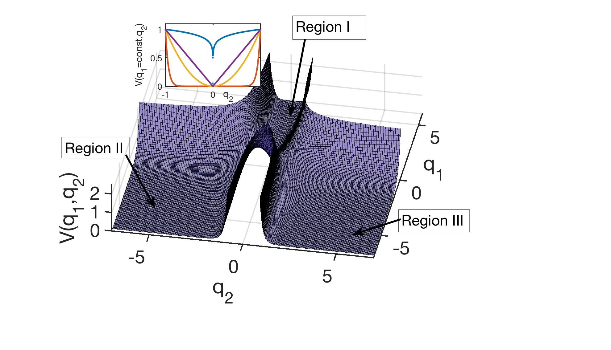
Figure 1: The potential energy landscape of a single interaction term $V(q_{1},q_{2})=|q_{2}|^{q_{1}}$. The CC (region I) as well as the two regions of asymptotically free motion, regions II and III, are indicated. The inset shows intersections of the potential energy along the $q_{2}$ coordinate i.e. $V(q_{1}=\mathrm{const},q_{2})$ for $q_{1}=0.1,1,2,16$ corresponding to the curves from top to bottom.

The SEP ${\cal{V}}(q_{1},q_{2},...,q_{N})=\sum_{k=2}^{N}|q_{k}|^{q_{1}}$ in eq.(1) possesses stationary points, i.e. zero derivatives $\frac{\partial{\cal{V}}}{\partial q_{i}}=0,\forall i=1,...,N$, at the positions $q_{1}=0,q_{i}=\pm 1,i=2,...,N$. The resulting Hessian possesses a zero determinant, but a more detailed analysis shows that the extrema have unstable and stable directions, i.e. they are saddle points. The energies of the extrema are $E={\cal{V}}(q_{1}=0,\{q_{i}=\pm 1\})=(N-1)$.

Since the Hamiltonian equations of motion belonging to the Hamiltonian (1) possess a singularity for $q_{1}<0,q_{i}=0,i=2,...,N$, we introduce a regularization parameter $\epsilon>0$ for the SEP which now reads ${\cal{V}}_{reg}(q_{1},q_{2},...,q_{N};\epsilon)=\sum_{k=2}^{N}(\sqrt{q_{k}^{2}+\epsilon})^{q_{1}}$. This facilitates the numerical integration of the corresponding Hamiltonian equations of motion which read

$${\dot{q_{i}}}=p_{i}\hskip 28.45274pti=1,...,N$$ (2)

$${\dot{p}}_{1}=-\sum_{k=2}^{N}\left(\sqrt{q_{k}^{2}+\epsilon}\right)^{q_{1}}\ln\left(\sqrt{q_{k}^{2}+\epsilon}\right)$$ (3)

$${\dot{p}}_{i}=-\left(\sqrt{q_{i}^{2}+\epsilon}\right)^{q_{1}-2}q_{1}q_{i}\hskip 28.45274pti=2,...,N$$ (4)

Typical values chosen for the numerical simulations are $\epsilon=10^{-8}$. The equation of motion for $p_{1}(t)$ depends symmetrically on all $q_{k},k=2,...,N$ due to the above-mentioned exchange symmetry. Note the appearance of the logarithm which will be of major importance for the later on observed dynamics. The equation of motion of $p_{i}(t),i=2,...,N$ depends only on the coordinates $q_{i}$ and $q_{1}$ and these equations ($i=2,...,N$) are structurally invariant due to the exchange symmetry. This means, that for equal initial conditions (ICs) of all $(q_{i},p_{i}),i=2,...,N$ at $t=t_{0}=0$ the dynamics of all $q_{i}(t),i=2,...,N$ will be identical.

Let us elaborate on this in some more detail since it allows us to identify a hierarchy of invariant subspaces that classify the dynamics. The exchange symmetry among the $N-1$ particles with respective coordinates and momenta $(q_{i},p_{i}),i=2,...,N$ can be either (i) completely broken (ii) partially broken or (iii) fully maintained by the corresponding ICs. We therefore partition the complete phase space of ICs into subspaces as follows. We divide the $2N-2$-dimensional total phase space ${\cal{P}}$ of the dof $q_{i},i=2,...,N$ into dynamically invariant subspaces ${\cal{C}}_{i}$ of identical ICs which lead consequently to an identical dynamics (trajectories). Here the invariance refers to the exchange of (initial) phase space coordinates in the corresponding subspace ${\cal{C}}_{i}$. These subspaces represent a classification of the dynamics. More specifically, we define a series of positive integers $\{n_{i}\}=n_{1},....,n_{k}$ with $\sum_{i=1}^{k}n_{i}=(N-1)$ where $n_{i}$ is the maximal dimension of the subspace ${\cal{C}}_{i}$ with identical initial phase space coordinates. A complete set of ICs (and resulting trajectories) is then given by the decomposition $\cup_{i=1}^{k}{\cal{C}}_{i}={\cal{P}}$. This set involves, per definition, $k$ different classes of identical trajectories, the $i-th$ class containing $n_{i}$ identical phase space coordinates. A remark concerning the resulting combinatorics is in order. For a single subset of $l$ identical ICs only there is $\binom{N-1}{l}$ possible configurations or subspaces with $l\leq(N-1)$. For $r$ subsets each one with $k$ identical ICs the number of possibilities is $\sum_{i=0}^{r-1}\binom{N-ik-1}{k}$. This generalizes to the case of an arbitrary number of subspaces of properly chosen dimensions with identical ICs.

III Dynamics: Individual Many-Body Trajectories

This section is devoted to the exploration of the many-body dynamics by analyzing individual trajectories which illustrate the relevant collisional processes. We note that these trajectories are representative and show the typical observed behaviour. The general procedure is as follows. We will simulate the dynamics in the CC (region I) for incoming ($p_{1}<0$) trajectories starting at $t=0$ in the outer part of the channel at $q_{1}=30$. At this value of $q_{1}$ the transverse profile of the channel represented by the intersections of the individual interaction potential terms ${\cal{V}}(q_{1}=\mathrm{const},q_{2})$ is already very similar to a box confinement. We will then study the dynamics with increasing total energy and for different subspaces of identical ICs.

III.1 Low energy scattering

Let us start by assuming that all ICs of the coordinates and momenta $(q_{i},p_{i}),i=2,...,N$ are identical. Since then (see discussion in section II) all dynamical evolutions $q_{i}(t),p_{i}(t)$ are identical this case is similar to the case of the corresponding superexponentially interacting two-body system Schmelcher4 . Let us summarize the main features and characteristics of the dynamics for the two-body case (where the total potential reads ${\cal{V}}=|q_{2}|^{q_{1}}$) for reasons of comparison to the actual many-body case. Since the exponent dof $q_{1}$ provides the confinement for the dof $q_{2}$ the time evolution of $q_{2}(t)$ shows bounded oscillations in the channel (see Figure 3(a) for a specific case of the many-body system). For large values of $q_{1}$ this confinement is strongly anharmonic and close to a box-like confinement: as a consequence the channel is approximately flat for $-1\lesssim q_{2}\lesssim+1$ and energy exchange processes (between particles but also from kinetic to potential energy for a single dof) happen only close to the turning points of the $q_{2}$ oscillations. Opposite to this the $q_{1}$-motion is not oscillatory and is unbounded. This can be argued as follows. Inspecting eq.(3) and specializing it to the case of a single base dof $q_{2}$ one realizes that the r.h.s. is positive ($\epsilon=0$) as long as the logarithm is negative, which implies $q_{2}<1$. A necessary condition for ${\dot{p_{1}}}<0$ to happen is then given by the occurence of $q_{2}>1$ which implies that the total energy $E>1$. The latter is however the energy of the saddle points in the two-body problem. To conclude, this means that for energies below the saddle point energies the two-body scattering in the CC involves a time evolution $q_{1}(t)$ with exclusively ${\ddot{q}}_{1}>0$ i.e. the incoming $q_{1}(t)$ trajectory possesses a single turning point ! As a consequence, $q_{1}(t)$ cannot perform an oscillatory bounded motion but describes simply a direct in-out scattering process finally escaping asymptotically to $q_{1}\rightarrow\infty$. In this sense multiple scattering processes are not encountered and scattering is not chaotic, i.e. there is even no transient dynamics with nonzero Lyapunov exponents. This situation changes when considering the many-body situation. Here the saddle point energy is given by $E_{s}=(N-1)$ and the dynamics of $(q_{1},p_{1})$ is determined (see eqs.(2,3)) by the sum over all forces involving the dof $q_{i},i=2,...,N$. This sum has to become overall positive (as a combination of the appearing logarithms and their ’above threshold’ $q_{k}>1,k\in\{2,...,N\}$ arguments) in order to enable ${\dot{p_{1}}}<0$ and to provide multiple turning points as well as an oscillatory dynamics: it is an inherent many-body process.

Figure 2(a) shows the kinetic energies $E_{k1}=\frac{p_{1}^{2}}{2}$ and $E_{ki}=\frac{p_{i}^{2}}{2}$ as well as the corresponding potential energies $E_{pi}=|q_{i}|^{q_{1}}$ (see inset) as a function of time for the scattering process of a system of $N=10$ particles with the total energy $E=0.28$. Here all ICs of the base dof are identical i.e. the particle exchange symmetry among the dof $q_{i},i=2,...,N$ is fully maintained and their dynamics is the same. Therefore, we expect that the above described properties of the two-body scattering dynamics should also appear here.

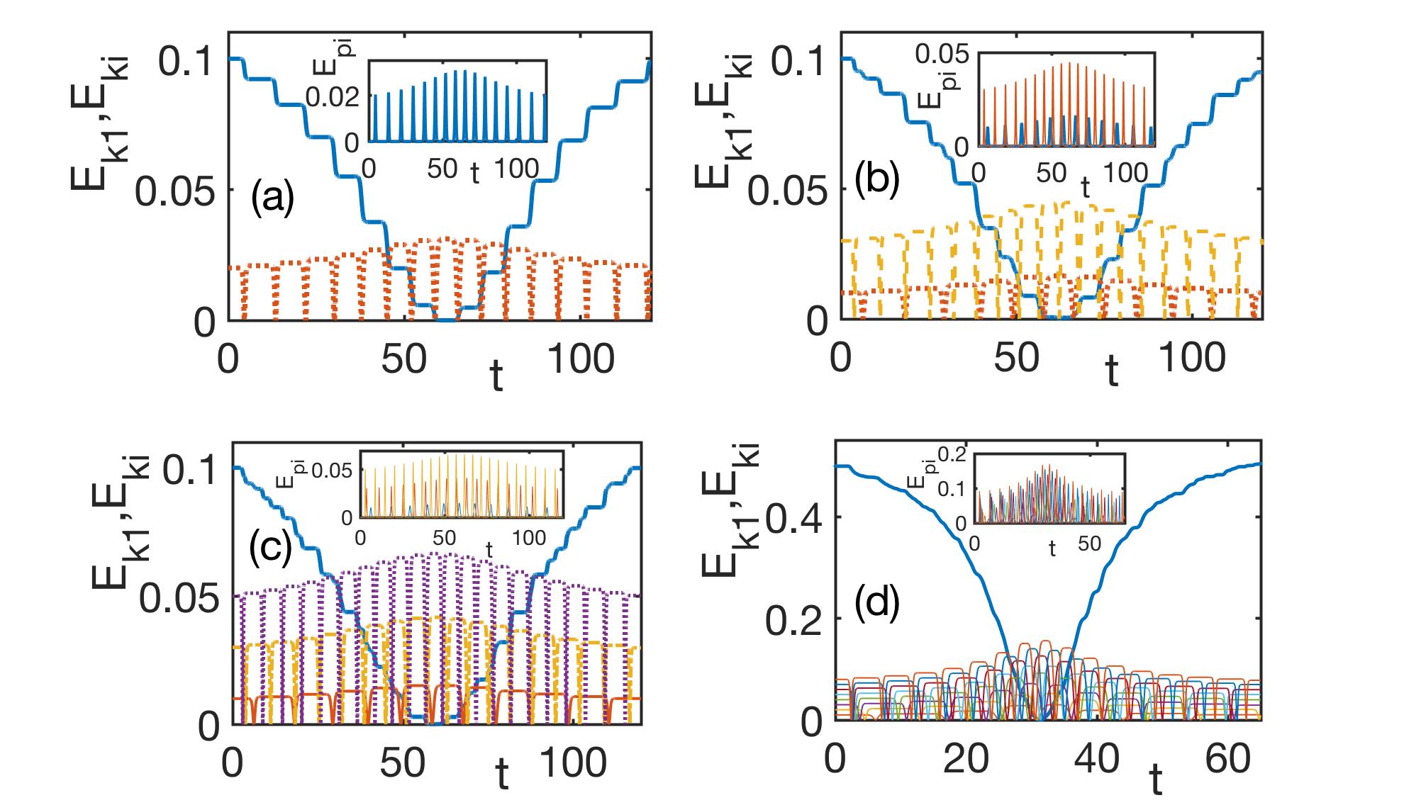
Figure 2: The kinetic energies $E_{k1}$ (blue solid curve), $E_{ki}$ (dotted, dashed and dot-dashed curves), and potential energies $E_{pi}$ (see inset), belonging to the dof $q_{1},q_{i}$, respectively, as a function of time $t$ for individual trajectories. Initial conditions are $q_{1}=30,q_{i}=0,i=2,...,N$. (a) Total energy $E=0.28$ and initial conditions $E_{k1}=0.1,E_{ki}=0.02$. Note that all curves $E_{ki},i=2,...,N$ are identical due to identical ICs. Similar statements hold for (b,c). (b) Total energy $E=0.29$ and initial conditions $E_{k1}=0.1$, $E_{ki}=0.01,i=2-5$, $E_{kj}=0.03,j=6-10$. (c) Total energy $E=0.37$ and initial conditions $E_{k1}=0.1$, $E_{ki}=0.01,i=2-4$, $E_{kj}=0.03,j=5-7$, $E_{kl}=0.05,l=8-10$, (d) Total energy $E=0.95$ and initial conditions $E_{k1}=0.5$, $E_{ki}=0.01\cdot(i-1),i=2-10$. All simulations involve $N=10$ particles.

Indeed, the initial kinetic energy $E_{k1}(t=0)=0.1$ belonging to the subsequent time evolution $(q_{1}(t),p_{1}(t)$ decreases monotonically to zero and subsequently increases in the course of the scattering process (see Figure 2(a)). $E_{k1}(t)$ exhibits a sequence of plateaus which correspond (see discussion above) to the traversal of $q_{i}(t)$ of the bottom of the CC, while the phases of rapid changes of $E_{k1}(t)$ between two plateaus is caused by the dynamics in the vicinity of the potential walls. These facts are consistent with the behaviour of the potential energy $E_{pi}$ (see inset of Figure 2(a)) which exhibits pronounced peaks during these collisions with the potential walls. For reasons of energy conservation $E_{ki}(t)$ show then corresponding dips.

As a next step let us break the (total) exchange symmetry among the base dof by firstly inspecting the case of two sets of identical ICs. Figure 2(b) shows the kinetic $E_{k1},E_{ki}$ and the potential energies $E_{pi}$ for a total energy $E=0.29$ and ICs $(E_{ki}=0.01,i=2-5);(E_{kj}=0.03,j=6-10)$. Since we have now two different sets of identical dynamics namely $(q_{i}(t),i=2-5);(q_{j}(t),j=6-10)$ a partial exchange symmetry remains. The corresponding time evolution $E_{k1}(t)$ carries now the signatures of two different transversal motions $(q_{i}(t),q_{j}(t))$: the overall decrease and subsequent increase due to the collision process exhibits now a ’superposition’ of plateau-like structures. Correspondingly, there is two different kinds of time evolution of kinetic energies $E_{ki}(t),E_{kj}(t)$ which show sharp dips at the time instants where the kinetic energy $E_{k1}(t)$ varies rapidly in between two plateaus. The associated potential energies $E_{pi}(t),E_{pj}(t)$ (see inset of Figure 2(b)) show pronounced peaks at the time instants of collisions with the potential walls which correspond to the time instants of the previously mentioned dips of $E_{ki}(t),E_{kj}(t)$.

Figure 3(a) shows the channel dynamics for the base and exponent dof $q_{1},q_{i},i=2,...,N$ and Figure 2(c) the corresponding kinetic and potential energies for a total energy $E=0.37$ for the case of three sets of identical ICs. The dynamics of $E_{k1}(t)$ shows a larger number of plateaus which, due to their partial overlap, gradually become washed-out. This becomes even more pronounced for the case of no identical ICs and a total energy $E=0.95$ shown in Figure 2(d): here the time evolution $E_{k1}(t)$ becomes almost smoothly decreasing and subsequently increasing, i.e. without any pronounced plateau-like structures. In Figures 2(c,d) the time evolutions of the kinetic energies $E_{ki}(t)$ show an increasing number of dips and in case of the potential energies $E_{pi}(t)$ an increasing number of peak structures (see corresponding insets). In Figure 2(d) there exists already a rather dense accumulation of peaks ($E_{pi}(t)$, see inset) and dips ($E_{ki}(t)$) due to the many collisions of the particles with dof $q_{i}(t)$ with the walls of the interaction potential ${\cal{V}}$.

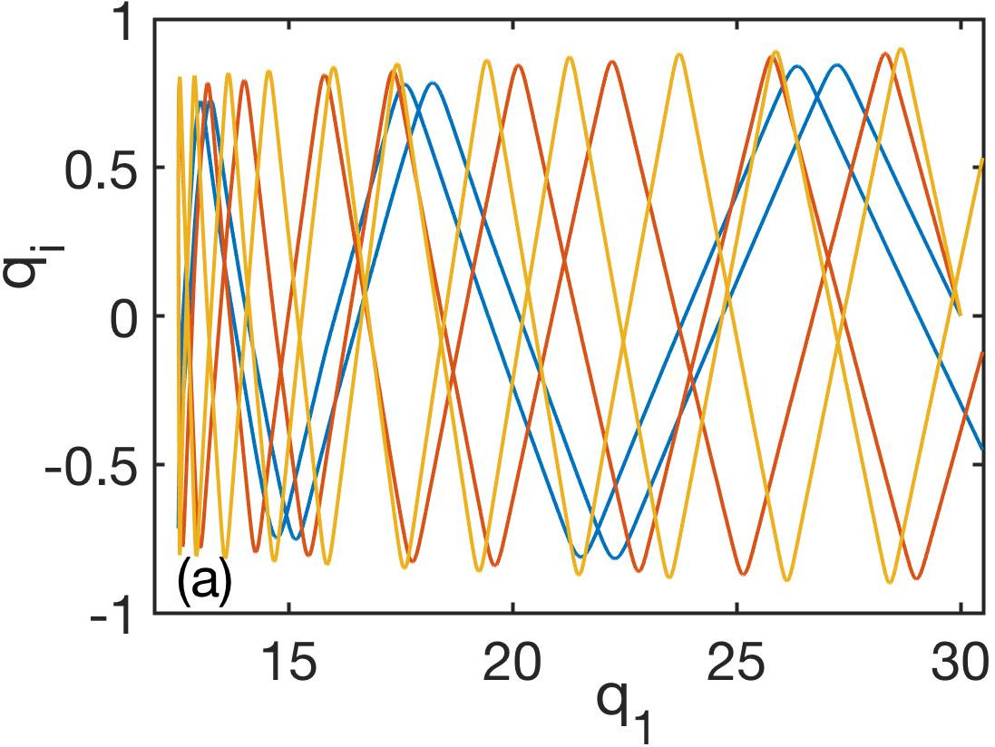
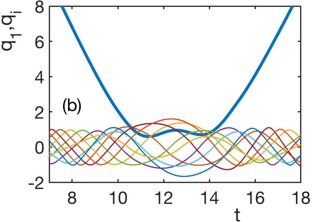
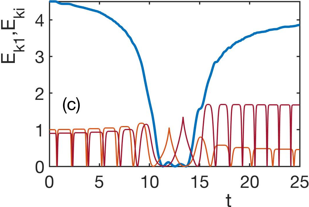
Figure 3: (a) A $(q_{1},q_{i})$ graph of scattering trajectories in the CC with initial conditions $q_{1}=30,q_{i}=0,i=2,...,N$ and $E_{k1}=0.1,(E_{ki}=0.01,i=2-4),(E_{kj}=0.03,j=5-7),(E_{kl}=0.05,l=8-10)$ and for a total energy $E=0.37$. Clearly visible are three types of transversal $q_{i}(t)$ oscillations and the reflection process at the minimal value of $q_{1}$. (b) Time evolution $q_{1}(t),(q_{i}(t),i=2,...,N)$ of a scattering trajectory with total energy $E=10.6$ via the CC. Initial conditions for the coordinates are the same as in (a), and $E_{ki}=4.5,1,0.4,0.7,0.9,1.1,0.5,0.8,0.6,0.1$ corresponding to $i=1,...,10$. An oscillatory behaviour in the saddle point region is clearly visible. (c) Same as in (b) concerning the parameters and ICs. Shown are the kinetic energies $E_{k1}(t),E_{ki}(t)$ for a few selected particles to get a representative view. Multiple oscillations and inelastic processes are evident.

III.2 Intermediate energy scattering

We remind the reader of the fact that the saddle point threshold energy is $E_{s}=(N-1)$ which amounts to $E_{s}=9$ for our prototypical 10 particle system. As discussed above (see section III.1) the two-body case as well as the case of identical ICs for all base dof (in the many particle case) show only a single turning point, i.e. a direct in-out scattering behaviour, for the exponent dof $q_{1}(t)$ for energies $E<E_{s}$. This statement holds also for the low energy scattering $E\ll E_{s}$ discussed in the previous subsection where a transition of the dynamics $E_{k1}(t)$ from plateau-dominated to a smooth behaviour has been observed with increasing number of different ICs.

Let us now increase the total energy available in the scattering process for non-identical initial conditions. A necessary condition for further turning points to occur in the dynamics of $q_{1}(t)$ is (see corresponding discussion in section III.1) the positivity of the logarithmic terms in the equation of motion (3) which implies that $q_{i}>1$ has to occur for some particles such that the overall sum becomes positive. Consequently certain interaction potential contributions obey $E_{pi}>1$. Figure 3(b) shows for an energy $E=10.6$ the dynamics $q_{1}(t),(q_{i}(t),i=2,...,N)$ of an example trajectory with no identical ICs. Here it is clearly visible that the dof $q_{1}(t)$ enters in the course of the scattering process from the CC to the saddle point region and performs thereafter an oscillation followed by an escape back into the CC. The dof $q_{i}(t),i=2,...,N$ show an increase of the amplitude of oscillations during the the dynamics in the saddle point region. Figure 3(c) shows the kinetic energy $E_{k1}(t)$ and exemplarily two of the kinetic energies $E_{ki}(t),i\neq 1$ for the same trajectory. $E_{k1}(t)$ shows according to the oscillation of $q_{1}(t)$ in the saddle point region an oscillation with three zeros. Inspecting the incoming and outgoing $E_{k1}(t),E_{ki}(t),i\neq 1$ the inelasticity of this scattering event for intermediate energies becomes visible: $E_{k1}$ and one of the $E_{ki}$ loose energy in the course of the scattering whereas the other $E_{ki}$ component gains energy. While this example trajectory possesses an energy $E>E_{s}$ the principal process that an oscillatory dynamics of $q_{1}(t)$ becomes now possible is by no means restricted to an energy above the saddle point energy. This is impressively demonstrated in Figure 4(a,b,c).

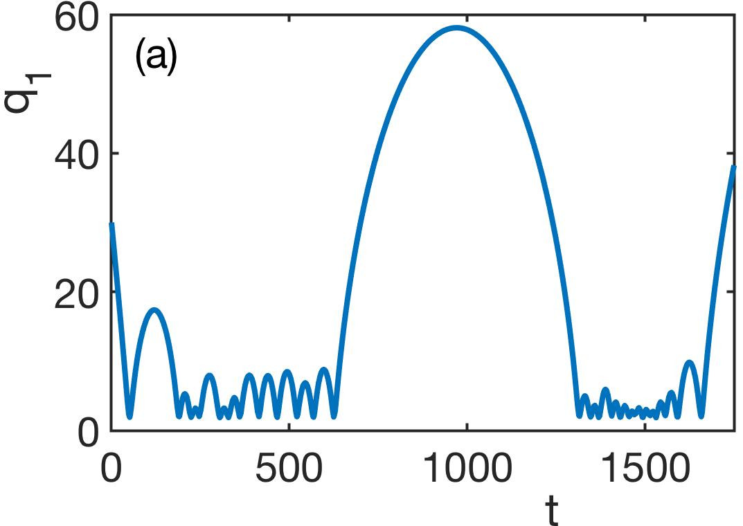
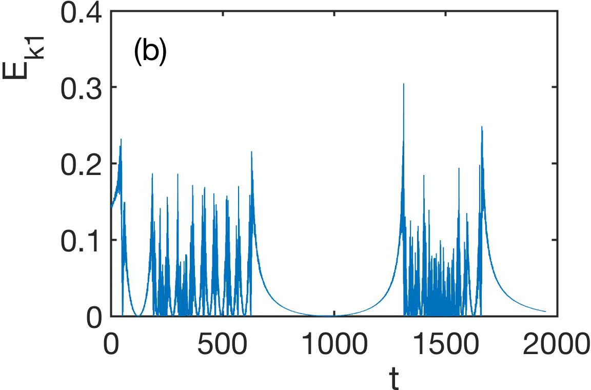
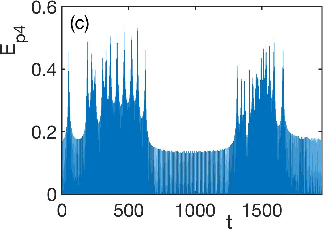
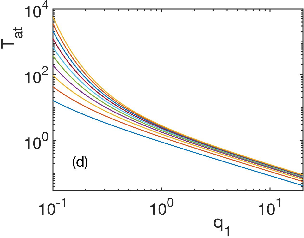
Figure 4: (a) Time evolution $q_{1}(t)$ of a scattering trajectory closely approaching the saddle point region and showing oscillations of largely different amplitudes. Initial conditions are $q_{1}=30,q_{i}=0,i=2,...,N$ and $p_{i}=-0.53,0.65,1.08,0.58,1.92,2.15,0.35,2.57,0.53,0.06$ and the total energy is $E=8.8$. (b) and (c) show the specific kinetic $E_{k1}(t)$ and potential $E_{p4}(t)$ energies. (d) The time $T_{at}$ spent above the threshold $q_{2}=1\leftrightarrow E=1$ within the single particle dynamics as a function of $q_{1}$. The curves from top to bottom correspond to the energies $E=2.0,...,1.1$ in steps of $0.1$.

Figure 4(a) shows the time evolution of $q_{1}(t)$ of a scattering trajectory emerging from $q_{1}(t=0)=30$ and traveling towards the saddle point region. Reaching the latter we observe a series of oscillations until, at time $t\approx 1700$, backscattering into the CC takes place with no further turning points to occur. The many oscillations taking place possess very different amplitudes. Indeed, the first oscillation has its turning point at $q_{1}\approx 18$ followed by a large number of oscillations with a significantly smaller amplitude. At $t\approx 600$ a huge amplitude oscillation with a turning point deep into CC is observed. Subsequently a series of small amplitude oscillations occurs until the final escape into the CC happens. We emphasize that such an intermittent behaviour involving backscattering and recollision events is completely absent for the corresponding two-body system but is an inherent feature of the many-body case. Although being a high-dimensional phase space, we could exemplarily show that this highly oscillatory behaviour traces unstable periodic orbits which occur in the saddle point region. This means once the trajectory gets close to one of those orbits it stays temporarily in its vicinity i.e. it temporarily shadows the unstable periodic motion.

A few remarks are in order. As emphasized above the corresponding two-body system shows only simple backscattering into the CC. Scattering trajectories of the many-body system can, however, show backscattering into the CC followed by recollision events. Once the system recollides it dwells in the saddle point regime and finally gets backscattered into the CC. Of course, since oscillations take place also for small amplitudes this is a crude picture of what happens indeed. According to the analysis in section III.1 a necessary condition for the occurence of a recollision event is the surpassing of the threshold value $q_{i}=1$ for some dof $i$. A closer inspection reveals that there is generically several transversal channel dof from the set $q_{i},i=2,...,N$ involved in this process: it is the sum on the r.h.s of eq.(3) which has to change sign in order to introduce the possibility of a recollision event. Indeed, the surpassing of the threshold value leads to a deceleration and finally a turning point in the dynamical evolution. Note that this process of repeated backscattering and recollision does not require a fine tuning but happens generically for the regime of intermediate energies below (and above, see next section III.3) the saddle point threshold energy $E_{s}$. We remind the reader of the fact that this oscillatory behaviour is a pure dynamical interaction effect and there is no stable equilibria of the potential landscape that would be responsible for these processes.

To get a simple measure for the probability that our dynamical system resides in the above-threshold regime $q_{i}>1$, which enables a pronounced deceleration dynamics and finally leads to an oscillatory behaviour, we take the following approach. We focus on the case of a single particle in the one-dimensional potential $V(q_{2};q_{1})=|q_{2}|^{q_{1}}$ with a constant value for the parameter $q_{1}>0$. Assuming $q_{2}>1$ means for the energy $E>1$. The time which the particle spends in this regime $q_{2}>1$ in the course of a positive half-period of its oscillation reads as follows

$$T_{at}=\sqrt{2}\int_{1}^{q_{t}}\frac{dq}{\sqrt{E-|q|^{q_{1}}}}$$ (5)

for $q_{t}=E^{\frac{1}{q_{1}}}$. Figure 4(d) shows $T_{at}$ as a function of $q_{1}$ which represents the power of the potential $V(q_{2};q_{1})$ for varying energy $E=1.1-2.0$ in steps of $0.1$. Obviously, $T_{at}$ is very small for large $q_{1}$ due to the box-like confinement and the steep walls which lead to a very short time spent in the course of the dynamics in the region $q_{2}>1$. $T_{at}$ increases strongly with decreasing value of $q_{1}$ - this increase is neither a power law nor an exponential one but of superexponential character. It reflects the flattening of the increase of the potential $V$ for $q_{2}>1$ in particular for $q_{1}<1$. With increasing energy the dependence of $T_{at}$ on $q_{1}$ becomes more pronounced. This analysis provides an intuitive explanation of the observation that the oscillations of the trajectories of the many-body system, i.e. the backscattering and recollision events, emanate from the saddle point region for which $q_{1}<1$ and where the particles possess a large dwell time in the ’reactive zone’ $q_{i}>1$.

Let us now return to our superexponential many-body system. Figure 4(b) presents the kinetic energy $E_{k1}(t)$ belonging to this heavily oscillating scattering trajectory. We observe that small amplitude oscillations involve high frequency energy exchange processes whereas large amplitude excursions into the CC involve low frequency oscillations of the kinetic energy. Since small amplitude oscillations (see $q_{1}(t)$ in Figure 4(a)) are interdispersed between large amplitude oscillations we correspondingly observe in Figure 4(b) bursts of high frequency kinetic energy oscillations interdispersed between intervals of smooth variations. Correspondingly a representative of the potential energy $E_{p4}$ is shown in Figure 4(c) which peaks whenever a collision with the confining walls takes place.

III.3 High energy scattering

We now turn to a discussion of the dynamics for energies above the saddle point threshold $E_{s}=(N-1)$. Due to the structure of our Hamiltonian (1) which possesses many base dof but only a single exponential dof $q_{1}$, the dynamics $q_{1}(t)$ determines whether backscattering into the CC or transmission to the regions II and III of asymptotically free motion happens. Indeed, either all particles are backscattered or transmitted - a splitting into partial backscattering and partial transmission is not possible.

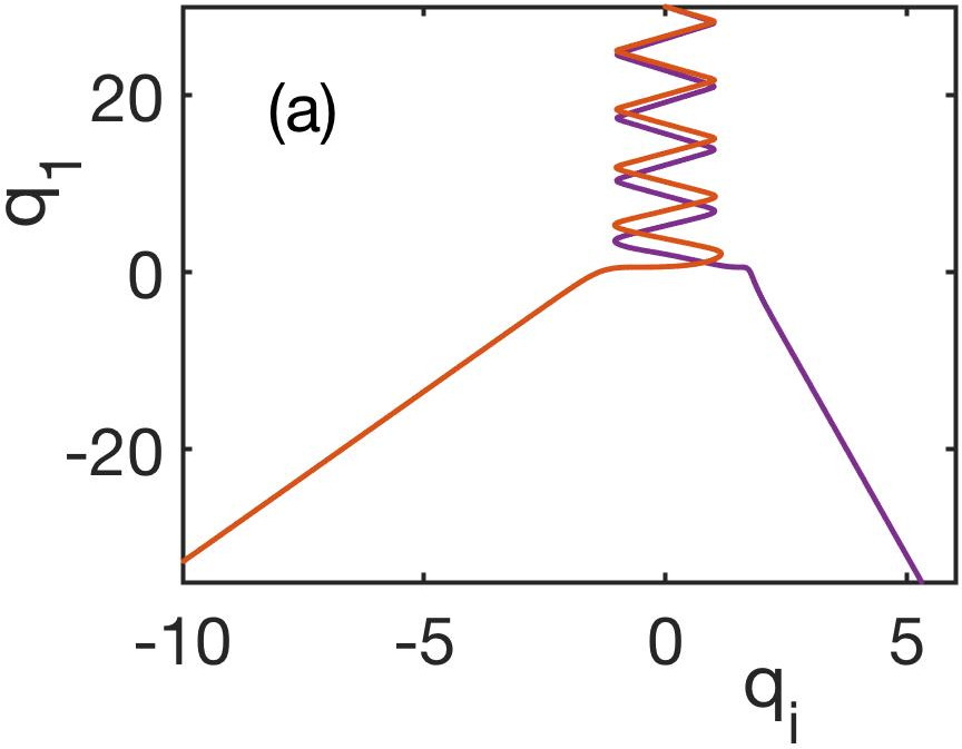
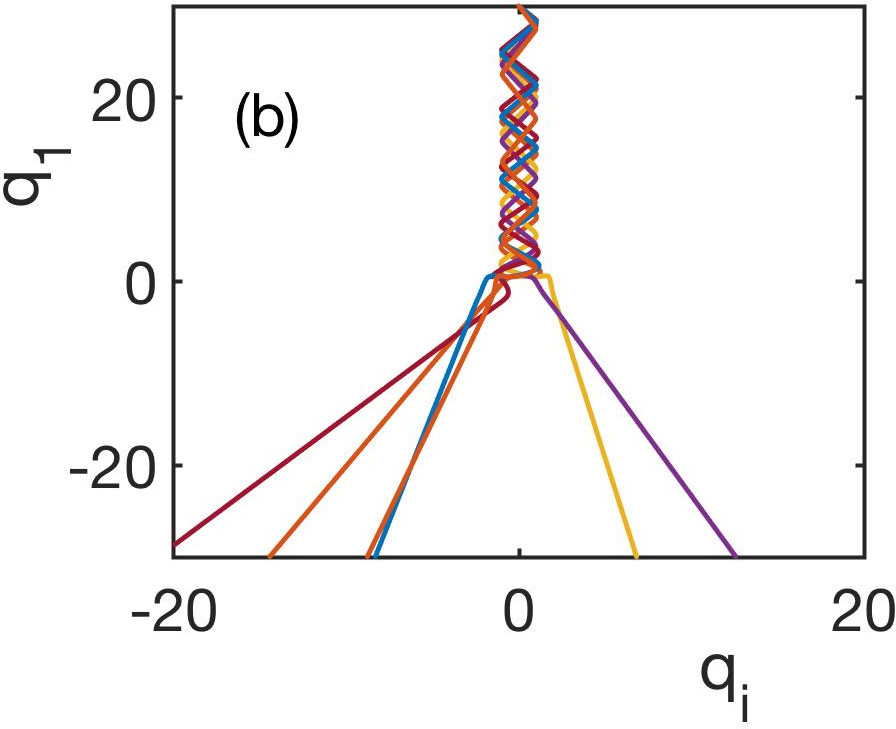
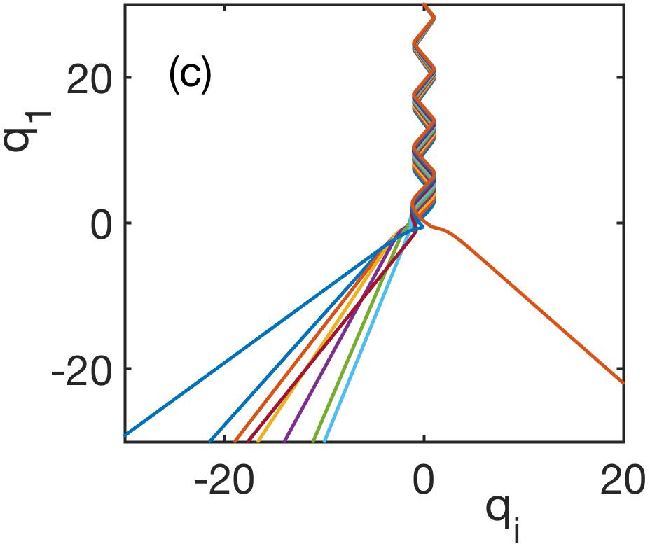
Figure 5: Transmitting trajectories in the $(q_{1},q_{i})$-plane above the saddle point energy $E_{s}=9$ for $N=10$ particles. ICs are $q_{1}=30,q_{i}=0,i=2,...,N$ and (a) $p_{1}=-2.45,(p_{i}=1.411;i=2-5),(p_{j}=1.55;j=6-10)$ for a total energy $E=13$ (b) $p_{i}=-2.45,1.18,1.41,1.27,1.18,1.61,1.48,1.61,1.48,1.00;i=1-10$ for a total energy $E=9.1$ as well as (c) $p_{i}=-2.82,1.45,1.48,1.52,1.55,1.58,1.61,1.64,1.67,1.70;i=1-10$ for a total energy $E=15.2$. From (a) to (c) the distribution of the particles onto the regions II and III of the potential landscape varies significantly.

Figure 5(a) shows a many-body trajectory in the $(q_{1},q_{i})$-planes for a total energy $E=13$, i.e. well above the saddle point energy $E_{s}=9$, and for two sets of identical ICs. Consequently two scattering processes are observed in Figure 5(a): the one set of identical ICs is scattered to region II and the other set to region III (see Figure 1). Figure 5(b) shows a trajectory in the $(q_{1},q_{i})$-planes for an energy $E=9.1$ slightly above the saddle point energy $E_{s}$ and for non-identical ICs except three sets of two identical ICs. In this case four scattering paths go to the region II whereas two enter the region III while overall transmission takes place. Finally Figure 5(c) shows a trajectory with energy $E=15.2$ with no identical ICs and as a result nine distinct paths can be observed. Eight of them go to region II and one to region III. The above clearly demonstrates that particles can be arbitrarily distributed, after passing the saddle point region, onto the regions II and III of asymptotic freedom. Dof with identical ICs, of course, show identical paths.

IV Dynamics: Statistical Properties

Let us now explore the statistical properties i.e. the behaviour of an ensemble of trajectories scattering in the CC of the superexponential potential landscape. Initial conditions are $q_{1}=30,q_{i}=0,i=2,...,N$, as in the case of the individual trajectories analyzed in the previous section, and we choose the kinetic energies $E_{ki},i=2,...,N$ randomly from a uniform distribution with the constraint to match the energy shell. First we analyze the case of identical ICs for the momenta $p_{2},...,p_{N}$, followed by the case of two sets of identical ICs and finally the case of all ICs being different. This way the particle exchange symmetry of the Hamiltonian is broken to an increasing extent by the chosen ICs. The main observables of our analysis are the so-called reflection time distribution (RTD) and the momentum-time map (MTM). The reflection time is the time interval a scattering trajectory needs to travel back to its starting-point in the CC at $q_{1}=30$. The RTD represents then a histogram of the distribution of these reflection times with varying initial conditions from the chosen ensemble. The MTM shows the intricate connection between the initial momentum $p_{1}$ and the reflection time for corresponding ensembles.

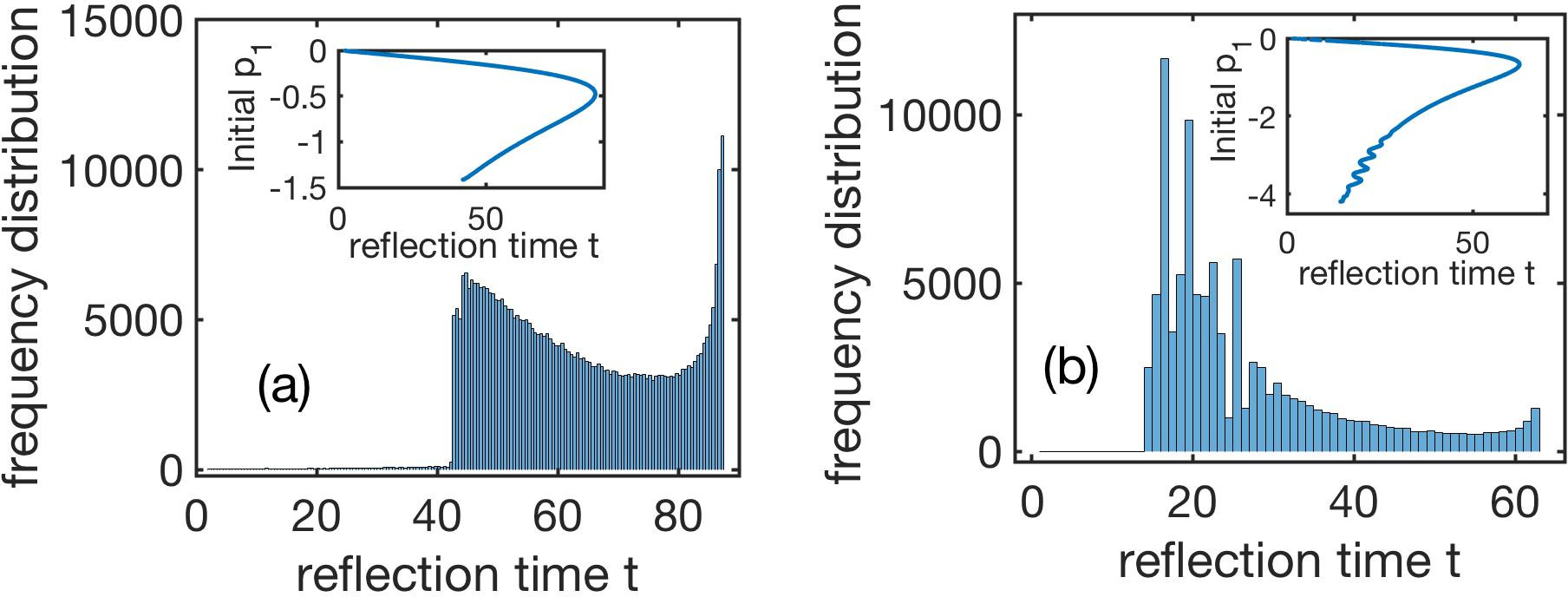
Figure 6: Reflection time distribution for scattering in the CC (region I). ICs are $q_{1}(t=0)=30,q_{i}(t=0)=0$. All further ICs for $p_{i},i=2,...,N$ are identical. (a) Parameters are $E=1,N=10$. The ensemble consists of $4\cdot 10^{5}$ trajectories with randomly chosen kinetic energies. Inset: The corresponding momentum-time map which provides the initial momentum $p_{1}$ versus the reflection time. (b) $E=8.8$ and the ensemble consists of $10^{5}$ trajectories with randomly chosen kinetic energies. Inset: The corresponding momentum-time map.

IV.1 Ensemble properties: Identical initial conditions

As discussed in section III.1 the case of identical ICs w.r.t. the momenta $p_{i},i=2,...,N$ for the many-body scattering dynamics is reminescent of the corresponding behaviour of the two-body superexponential scattering dynamics as discussed in detail in ref.Schmelcher4 . Nevertheless, for reasons of comparison to the generic symmetry-broken case of non-identical ICs we summarize here the main characteristics of this case. Figure 6(a,b) show the RTD and MTM for a low energy $E=1$ (a) and an energy $E=8.8$ (b) close to the saddle point energy $E_{s}=9$. The most striking observation in Figure 6(a) is the appearance of two plateaus. For the first plateau given by the range $0<t\lesssim 42.5$ the typical values of the RTD are by several orders of magnitude smaller as compared to the corresponding values in the range $42.5<t<87.5$ of the second plateau. Finally a prominent peak occurs at $t\approx 87.5$. The second plateau exhibits a broad valley towards this dominant peak.

The origin of the above-described features of the RTD can be understood by inspecting the corresponding MTM which is shown in the inset of Figure 6(a). The appearance of the MTM, i.e. whether it is e.g. a (single-valued) curve or a spreaded point pattern, is not determined a priori. The inset of Figure 6(a) shows that the MTM for the present case is a well-defined curve. For reflection times $0<t\lesssim 42.5$, this curve is single-valued whereas for $42.5<t<87.5$ it is double-valued, i.e. there appear two momentum branches of the MTM. These two regimes correspond to the first and the second plateau of the RTD (see main figure 6(a)). The time instant of the appearance of the second branch in the MTM with increasing reflection time is the time of the appearance of trajectories that travel to the origin of the SEP in the saddle point region and back. The lower branch for strongly negative values of the momentum $p_{2}$ provides the dominant contribution to the RTD for $t>42.5$ providing much larger values as compared to the contribution provided by the upper branch for $t<42.5$. The prominent peak at $t\approx 87.5$ can be understood by the observation that the MTM possesses at this maximal reflection time a vertical derivative: The integrated contribution to the RTD is therefore particularly large. This explains the overall appearance of the RTD. For more details we refer the reader to ref.Schmelcher4 .

Figure 6(b) shows the RTD and MTM (see inset) for an energy $E=8.8$ close to, but still below, the saddle point energy. For $0<t<13.6$ the RTD is strongly suppressed. It shows for $t\gtrsim 13.6$ a series of peaks followed by a smooth decay up to $t\approx 63$. These peaks stem from the small scale oscillations present in the MTM (see inset) near the onset of its second branch.

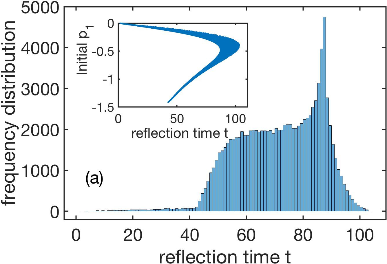
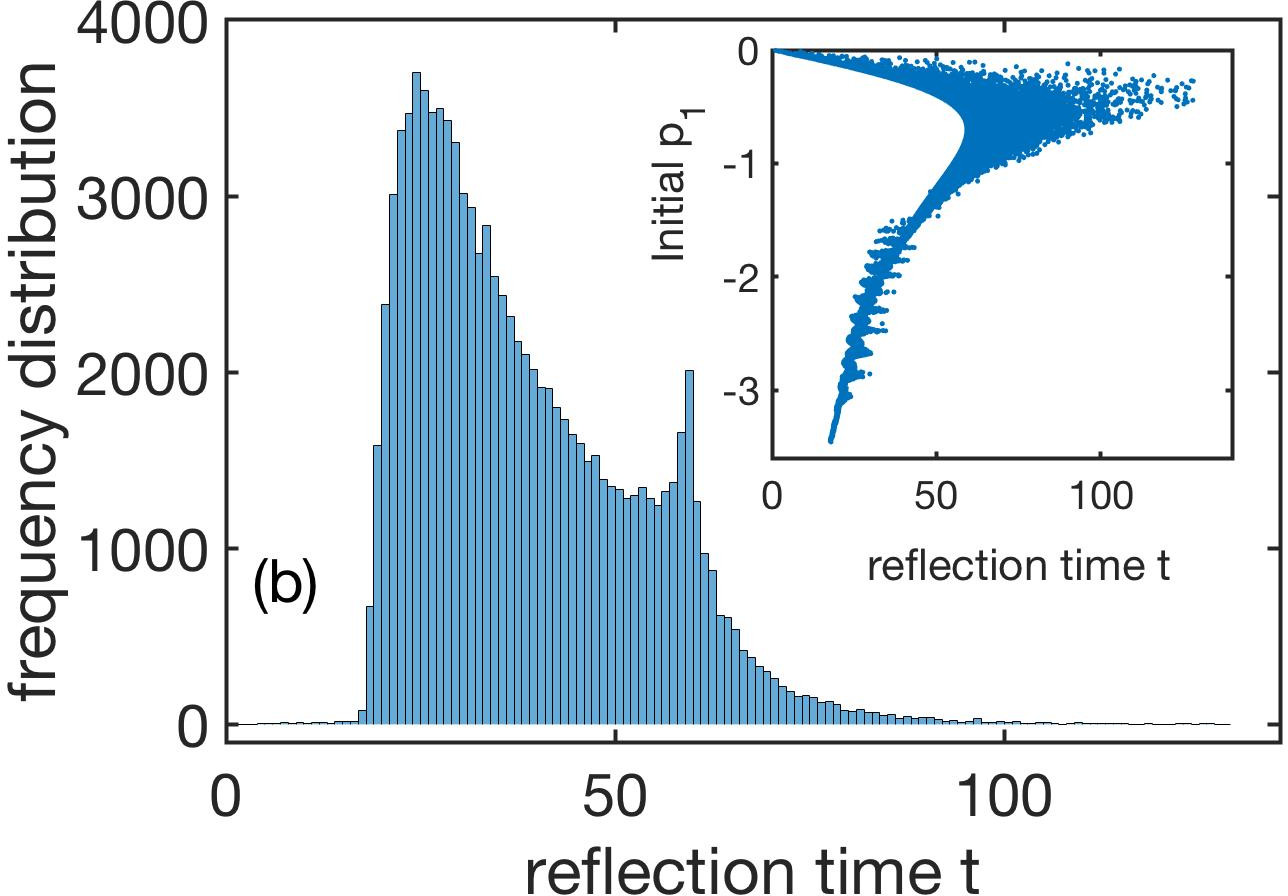
Figure 7: Reflection time distribution for scattering in the CC (region I). ICs are $q_{1}(t=0)=30,q_{i}(t=0)=0$. All further ICs of the dof $q_{i},i=2,...,N$ belong to two classes of identical ICs. (a) Parameters are $E=1,N=10$. The ensemble consists of $10^{5}$ trajectories with randomly chosen kinetic energies. Inset: The corresponding momentum-time map which provides the initial momentum $p_{1}$ versus the reflection time. (b) Same as (a) but for $E=6$. Inset: The corresponding momentum-time map.

IV.2 Ensemble properties: Two classes of initial conditions

Let us now analyze the RTD for a random ensemble of trajectories that possess two sets of identical ICs for $p_{i},i=2,...,N$, i.e. the particle exchange symmetry of the Hamiltonian is partially broken. These ICs of the coordinates of these trajectories obey $q_{1}=30,q_{i}=0,i=2,...,N$ as in section IV.1. Figure 7(a) shows the RTD for an energy $E=1$. Again two plateaus can be observed: the first one for $0<t\lesssim 43$ with a very low probability and a second plateau for $43\lesssim t<104$. Opposite to the case of all identical ICs the increase from the first to the second plateau as well as the decrease following the main peak is much smoother. The second plateau is essentially flat and possesses no undulation (compare to Figure 6(a)). These changes can be traced back to the corresponding changes in the MTM which is shown as an inset in Figure 7(a). We remind the reader that the MTM for all identical ICs concerning $p_{i},i=2,...,N$ represented a curve with two-branches (see inset of Figure 6(a)). The present MTM shows a similar overall structure but the branches possess now a finite width which increases with increasing reflection time. Again, the appearance of the second branch is responsible for the onset of the second plateau, but now the continuous increase of the widths of the branches leads to the observed smoothened behaviour of the RTD. Equally the smooth decay following the main peak of the RTD at $t\approx 88$ is due to the substantial extension of the MTM following the contact of the two distinct branches, i.e. for reflection times $t>88$.

Figure 7(b) shows the RTD and MTM (see inset) for a significantly larger energy $E=6$. Compared to the case $E=1$ (Figure 7(a)) a major reshaping of the RTD has taken place. The two regions of reflection times with largely different probabilities (plateaus) are still present, but the second plateau has become a highly asymmetric, broad and dominant peak with a maximum at $t\approx 25$. The peak at $t\approx 60$ where the two branches of the MTM fuse (see inset of Figure 7(b)) has decreased significantly. The features of the RTD can again be interpreted in terms of the significantly changed shape of the MTM: the onset of the second branch possesses a very steep slope and this branch exhibits for increasing reflection times $t\gtrsim 25$ a series of ’spread transversal oscillations’. This adds up to the broad asymmetric peak of the RTD.

IV.3 Ensemble properties: Mutually different initial conditions

Let us now address the statistics of an ensemble for which all ICs of $p_{i},i=2,...,N$ are different which refers to the case of a completely broken particle exchange symmetry of the Hamiltonian. Figure 8(a) shows the RTD and in the inset the corresponding MTM for an energy $E=1$. The plateau-like structure observed in sections IV.1 and IV.2 for the unbroken and partially exchange symmetry-broken cases, respectively, is now absent and is replaced by a single strongly asymmetric peak centered at $t\approx 90$. With increasing reflection times the RTD shows an accelerated increase culminating in the one central peak while decreasing rapidly thereafter. The underlying MTM (see inset of Figure 8(a)) shows the typical boomerang-like structure with two broadened branches. The first branch is widening systematically from its start at $t=0$ which is responsible for the substantial increase of the RTD for low reflection times.

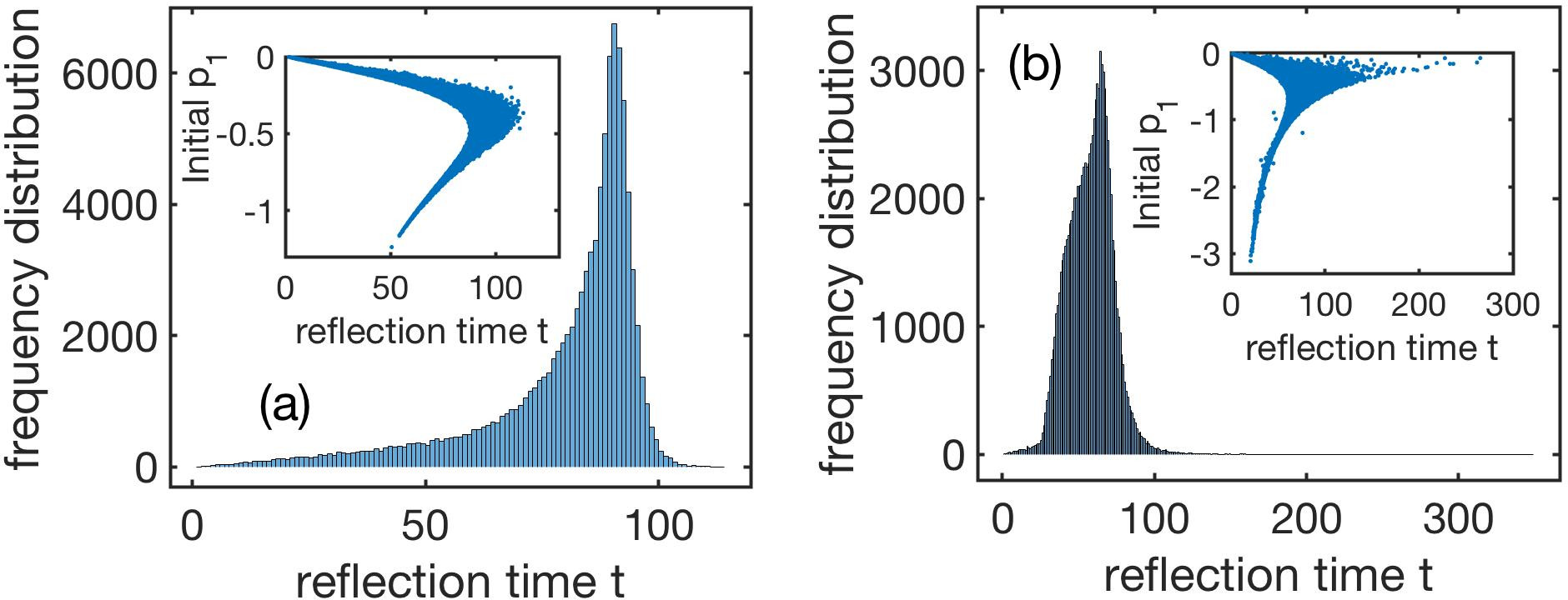
Figure 8: Reflection time distribution for scattering in the CC (region I). ICs are $q_{1}(t=0)=30,q_{i}(t=0)=0$. All further ICs (kinetic energies) of the dof $q_{i},i=2,...,N$ are different from each other. (a) Parameters are $E=1,N=10$. The ensemble consists of $10^{5}$ trajectories with randomly chosen kinetic energies. Inset: The momentum-time map. (b) Same as (a) but for $E=6$. Inset: The momentum-time map.

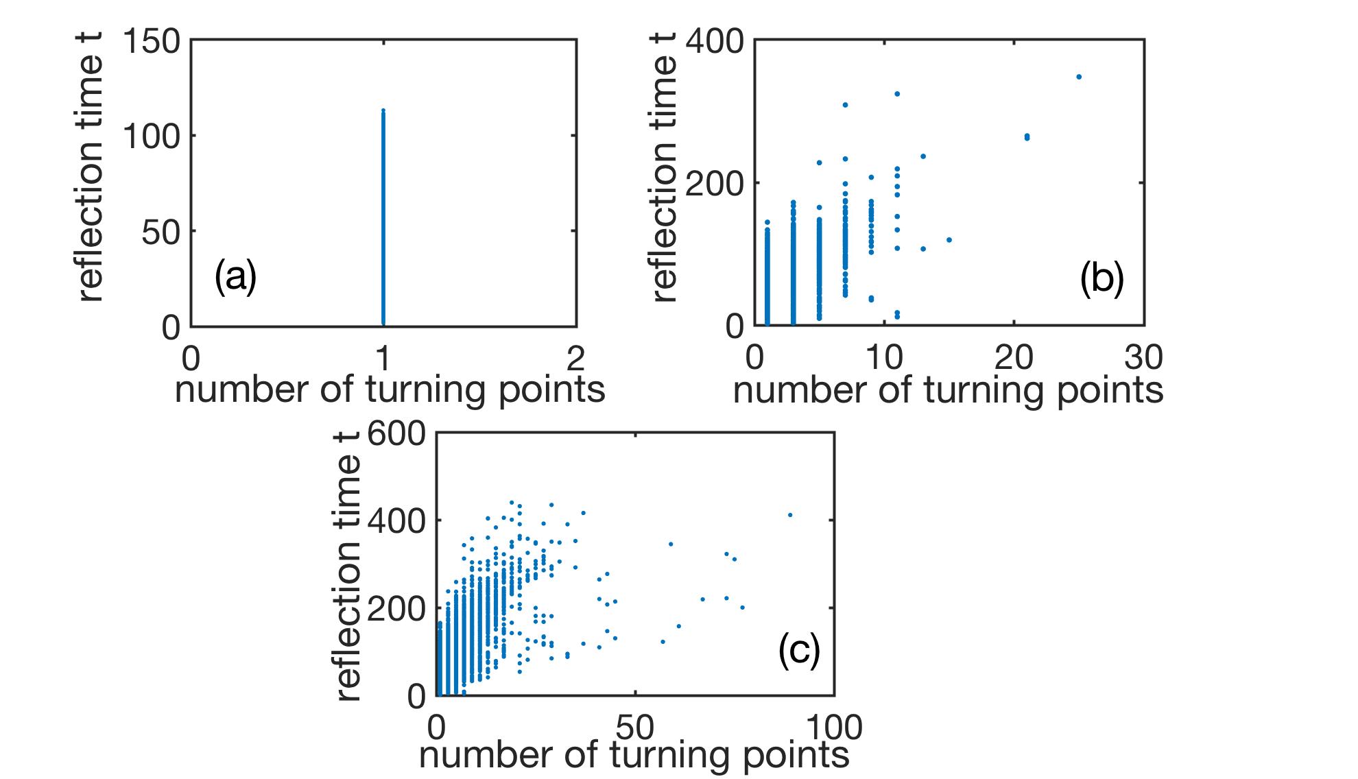
Figure 9: Reflection time versus number of turning points of the $q_{1}(t)$-motion for $E=1,6,8.8$ in (a,b,c), respectively, for an ensemble of $10^{5}$ trajectories. ICs as in Figure 8.

Figure 8(b) shows the RTD and MTM for an energy $E=6$. The main differences compared to the case $E=1$ is the reshaping of the asymmetric peak and the emergence of a very dilute tail for large reflection times. This is reflected in the strongly distorted MTM shown in the inset of Figure 8(b). The steep rise of the peak of the RTD for low reflection times emerges again from the large slope of the second branch of the MTM. The diffuse tail of the RTD has a corresponding counterpart in the MTM for large reflection times.

IV.4 Ensemble properties: Turning point distributions

In section III we have investigated our superexponential many-body Hamiltonian by analyzing the dynamics in terms of individual trajectories. The underlying basic two-body system Schmelcher4 shows a scattering dynamics without oscillatory behaviour w.r.t. the exponential dof, i.e. $q_{1}(t)$ possesses for energies below the saddle point energy only a single turning point which occurs at the minimal distance of the trajectories from the center of the SEP at $q_{1}=0$. In section III.2 we have shown that a major novelty in the many-body case is the oscillating structure with largely fluctuating amplitudes of trajectories experiencing the saddle point region or physically speaking the occurrence of multiple backscattering and recollision events. Let us now analyze the map between the reflection time of a trajectory and its number of turning points, which we call the RTPM, for the case of mutually different IC w.r.t. the momenta $p_{i},i=2,...,N$.

Figure 9(a) shows the RTPM for the energy $E=1$ for the scattering dynamics in the CC. Clearly, all trajectories and scattering events exhibit only a single turning point, and no oscillatory dynamics is encountered. The corresponding reflection times vary continuously from zero up to a maximal value $t\approx 114$. Increasing the energy to $E=6$ Figure 9(b) presents the corresponding RTPM which shows now a large number of events up to $9$ turning points and a few further events up to $25$ turning points. Note, that the number of turning points is always odd due to the fact that scattering takes place in the CC parametrized by the coordinate $q_{1}$. As a general tendency one observes that the reflection time increases with the number of turning points which is natural due to the fact that the dwell time in the saddle point region increases with increasing number of oscillations taking place in or traversing this region. Finally Figure 9(c) shows the RTPM for the energy $E=8.8$ rather close to the threshold energy $E_{s}=9$. As compared to the case of $E=6$ the number of turning points possible now extends even up to approximately $90$, while the absolute majority of events lies below $21$ turning points.

V Summary and conclusions

Model systems with superexponential interaction represent a peculiar type of dynamical systems with uncommon properties. Already for a two-body system the potential landscape shows a crossover from a confining channel (CC) with a strongly varying transversal profile via two saddle points to a region of asymptotic freedom. The scattering dynamics in the CC is intricate but at the same time restricted in the sense that it is a direct in-out scattering with a single turning point of the longitudinal channel coordinate $q_{1}$. This situation changes fundamentally when passing to many-body systems. In the present approach we have chosen a model system with a single exponent degree of freedom $q_{1}$ for the superexponential interactions and many base degrees of freedom $q_{i},i=2,...,N$. The exponential dof $q_{1}$ might be considered as a ’background’ or a ’guiding’ dof that determines the potential felt by the base dof. Each of the interaction terms $|q_{i}|^{q_{1}}$ shows the above-described geometrical crossover from channel confinement to asymptotic freedom. The many-body Hamiltonian exhibits a particle exchange symmetry of the dof $q_{i},i=2,...,N$ which can be respected, partially broken, or completely broken by the initial conditions.

Simulating the dynamics of the many-body system we have revealed a number of important differences to the two-body case. For low energies in the CC the $q_{1}(t)$ dynamics shows a transition from a step-like behaviour due to the spatially localized energy transfer processes to a smooth in-out scattering transition. Increasing the energy the trajectories incoming from the CC exhibit an oscillatory behaviour emanating from the saddle point region and possessing largely fluctuating amplitudes. This oscillatory dynamics comprised of backscattering and recollision events becomes increasingly more pronounced with increasing energy. It represent an inherent many-body effect since, generically, all of the dof $q_{i},i=2,...,N$ contribute to this process. We have analyzed this on the level of individual trajectories but also for the case of statistical ensembles. Here the reflection time distribution shows a characteristic transition from a two plateau structure to a single asymmetric peak behaviour. The latter has been analyzed by inspecting the so-called momentum-time map which shows a transition from a one-dimensional curve with two-branches to a spatially two-dimensional distribution with a characteristic shape.

There are several directions for possible future research on superexponential few- and many-body systems. The generalization of the interaction potential to higher spatial dimensions might lead to an even more intricate potential landscape with novel properties. The present case of a single exponent degree of freedom and many base degrees of freedom is certainly a specific choice, and it is an intriguing perspective to explore the case of several exponent degrees of freedom. An intriguing topic is the statistical mechanics of our many-body system in the thermodynamical limit, where one could pose the question whether superexponential systems relax to a stationary state of thermal equilibrium. Finally quantum superexponentially interacting systems resulting from a canonical quantization of the many-body Hamiltonian might show interesting scattering properties in particular due to the squeezing channel structure and the saddle point crossover.

VI Acknowledgments

The author thanks F.K. Diakonos for helpful discussions and B. Liebchen for a careful reading of the manuscript.

References

- (1) J.D. Jackson, Classical Electrodynamics, 3rd ed., Wiley (1998).
- (2) H. Friedrich, Theoretical Atomic Physics, Springer International Publishing 4th ed. 2017.
- (3) A.J. Stone, Intermolecular Forces, 2nd ed., Oxford University Press (2013).
- (4) J. Sirker, R. G. Pereira, and I. Affleck, Phys. Rev. B 83, 035115 (2011).
- (5) T. Giamarchi, Quantum Physics in One Dimension, Oxford University Press, (2003).
- (6) N.T. Zinner, Few-Body Systems 55, 599 (2014).
- (7) L. Samaj and Z. Bajnok, Introduction to the Statistical Physics of Integrable Many-Body Systems, Cambridge University Press (2013).
- (8) T. Busch, B.G. Englert, K. Rzazewski, M. Wilkens, Found. Phys. 28, 549 (1998).
- (9) M. Girardeau, J. Math. Phys. 1, 516 (1960).
- (10) C.J. Pethick and H. Smith, Bose-Einstein Condensation in Dilute Gases, Cambridge University Press, 2nd ed. (2008).
- (11) L.P. Pitaevskii and S. Stringari, Oxford University Press (2003).
- (12) P. Schmelcher, Phys. Rev. E 98, 022222 (2018).
- (13) P. Schmelcher, J.Phys.A 53, 075701 (2020).
- (14) P. Schmelcher, J.Phys.A 53, 305301 (2020).
- (15) P. Schmelcher, acc.f.publ. in Communications in Nonlinear Science and Numerical Simulation, https://doi.org/10.1016/j.cnsns.2020.105599
- (16) V. Gelfreich and D. Turaev, J. Phys. A 41, 212003 (2008).
- (17) K. Shah, D. Turaev and V. Rom-Kedar, Phys. Rev. E 81 056205 (2010).
- (18) B. Liebchen, R. Buechner, C. Petri, F.K. Diakonos, F. Lenz and P. Schmelcher, New J. Phys. 13, 093039 (2011).
- (19) K. Shah, Phys. Rev. E 88, 024902 (2013).
- (20) V. Gelfreich, V. Rom-Kedar, K. Shah and D. Turaev, Phys. Rev. Lett. 106, 074101 (2011).
- (21) V. Gelfreich, V. Rom-Kedar and D. Turaev, Chaos 22, 033116 (2012).
- (22) B. Batistic, Phys. Rev. E 90, 032909 (2014).
- (23) T. Pereira and D. Turaev, Phys. Rev. E 91, 010901 (R) (2015).