Drone classification from RF fingerprints using deep residual nets

Abstract

Detecting UAVs is becoming more crucial for various industries such as airports and nuclear power plants for improving surveillance and security measures. Exploiting radio frequency (RF) based drone control and communication enables a passive way of drone detection for a wide range of environments and even without favourable line of sight (LOS) conditions. In this paper, we evaluate RF based drone classification performance of various state-of-the-art (SoA) models on a new realistic drone RF dataset. With the help of a newly proposed residual Convolutional Neural Network (CNN) model, we show that the drone RF frequency signatures can be used for effective classification. The robustness of the classifier is evaluated in a multipath environment considering varying Doppler frequencies that may be introduced from a flying drone. We also show that the model achieves better generalization capabilities under different wireless channel and drone speed scenarios. Furthermore, the newly proposed model’s classification performance is evaluated on a simultaneous multi-drone scenario. The classifier achieves close to 99$\%$ classification accuracy for signal-to-noise ratio (SNR) 0 dB and at -10 dB SNR it obtains 5$\%$ better classification accuracy compared to the existing framework.

I Introduction

3GPP

3^rd Generation Partnership Program

CNN

Convolutional Neural Network

DNN

Deep Neural Network

DL

Deep Learning

DRNN

Deep Residual Neural Network

RELU

rectified linear unit

SeLU

scaled exponential linear units

RC

radio control

FC

fully connected

RPAS

remotely piloted aircraft systems

GAP

global average pooling

GCS

ground control station

FBMC

Filter Bank Multicarrier

PHY

physical layer

PU

Primary User

RAT

Radio Access Technology

RFNoC

RF Network on Chip

SDR

Software Defined Radio

SU

Secondary User

TOA

Time of Arrival

TDOA

Time Difference of Arrival

USRP

Universal Software Radio Peripheral

AMC

Automatic Modulation Classification

LSTM

Long Short Term Memory

SoA

state-of-the-art

FFT

Fast Fourier Transform

WSN

Wireless Sensor Networks

IQ

In-phase and quadrature phase

SNR

signal-to-noise ratio

sps

samples/symbol

AWGN

Additive White Gaussian Noise

DSSS

Direct Sequence Spread Spectrum

GoF

Goodness-of-Fit

FHSS

Frequency Hopping Spread Spectrum

OFDM

Orthogonal Frequency Division Multiplexing

LOS

line of sight

PSD

Power Spectral Density

SVM

Support Vector Machines

XGBoost

Extreme Gradient Boosting

AAE

Adversarial Autoencoder

VAE

Variational Autoencoder

SAIFE

Spectrum Anomaly Detector with Interpretable FEatures

ROC

Receiver operating characteristic

RNN

Recurrent Neural Network

AUC

Area Under Curve

DSA

Dynamic Spectrum Access

HMM

Hidden Markov Models

IoT

Internet of Things

API

Application Programming Interface

GNSS

Global Navigation Satellite System

COBRAS

Constraint-based Repeated Aggregation and Splitting

SSDO

Semi-Supervised Detection of Outliers

OSVM

One class Support Vector Machine

IFO

Isolation Forest

LOF

Local Outlier Factor

RCOV

Robust Covariance

RF

radio frequency

LODA

Lightweight on-line detector of anomalies

ARI

Adjusted Rand Index

Mini remotely piloted aircraft systems (RPAS) are imposing threats to national security. In recent years, the threat has become increasingly vivid due to the wide availability of low-cost drones. Several illicit incidents at security-sensitive places such as airports, national campaigns, international sports events and nuclear power plants [1] have been recorded. The conventional radar, video and acoustic detection systems may fail to detect and identify a drone, due to the small radar cross section, its resemblance to a bird or absence of LOS for vision based schemes, weather or daylight conditions and presence of high noise for acoustic systems [2]. On the contrary, an RF-based detection can work even in NLOS conditions, independent of the object size and daylight or weather condition and is capable to detect a drone from several kilometers away.

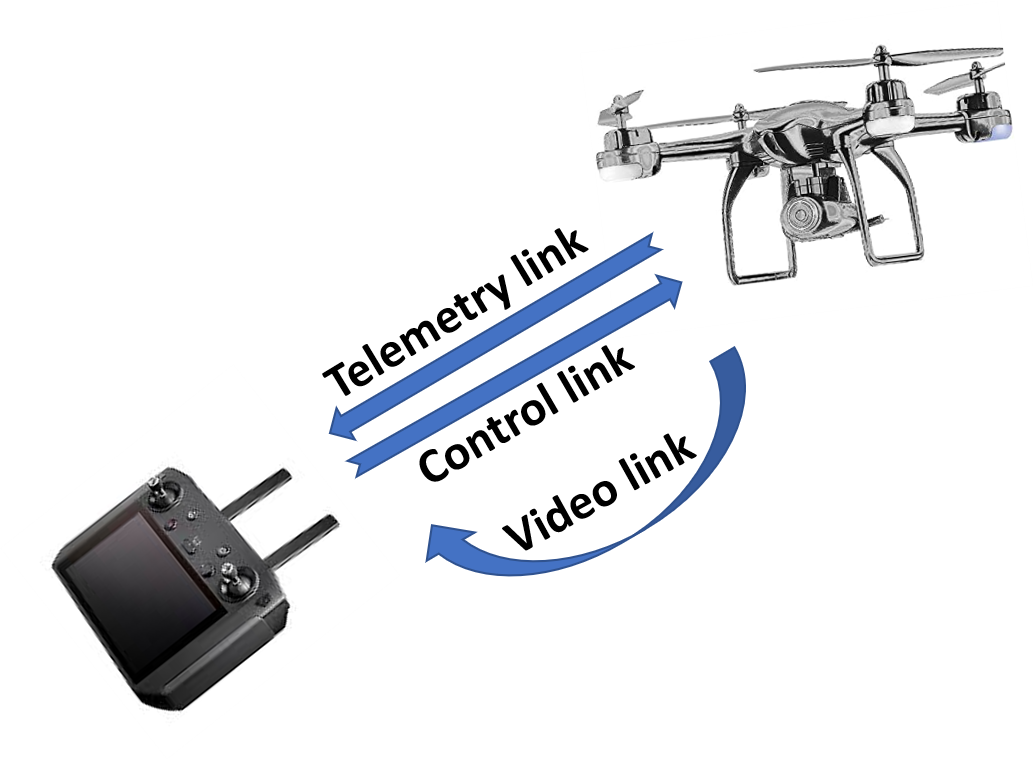
Figure 1: Drone RF communication

Several RF sensing based drone detection techniques have been proposed in the literature [3, 4, 5]. A joint active and passive drone detection and tracking system is proposed in [3], where the detection is performed through passive RF sensing at 2.4 GHz. In order to get the radio control (RC) signal and to update its status, most of the drones communicate with the ground control station (GCS) at every 33 ms approximately [6], whereas mobile devices and access points (APs) exchange beacons at every 100 ms [7]. This criteria was used in [3] to detect the presence of a drone. It was found in [3] that due to the motor rotation, camera feed, the propeller rotation and the communication channels of a flying drone, an RF emission happens within a frequency range from 20 Hz to 100 Hz. The identification of a drone was performed in [3], by sensing a frequency range of 20 Hz to 100 Hz. In [4], the drone identification was performed by measuring the packet length in bytes transmitted by a drone. However, these are inefficient methods, since, (a) any device transmitting at 30 times/sec or transmitting packets of similar length can fool the detector into believing that the signal is coming from a drone, (b) RF signal emission from a drone below 100 Hz is not an active communication signal, therefore, the detection based on this signal will be limited up to a short distance, (c) Multiple drones can transmit signals at the same rate with a similar packet length. Therefore, for robust drone classification, it is important to take into account the time and frequency domain RF signatures of a drone signal. We argue that the physical layer RF signatures are more usable than MAC layer and other passive signal emissions.

In [5], the authors utilized frequency domain signatures to detect and classify multiple drones. The authors have used a three layer fully connected (FC) Deep Neural Network (DNN) to detect and identify a drone. The analysis was only performed with three drone signals and the classification of the drone signals was not performed. Alongside the impact of noise and channel variations on the detection and the identification performance was not demonstrated. An efficient classification method is not only necessary for drone localization, this is also required for a smart jammer to neutralize a drone’s signal without interrupting other communications. The classification can also provide an insight about the type (e.g fixed wing or quadcopter) and size of drone. The drone communications are performed in the ISM bands and the ISM bands are generally occupied by several heterogeneous sources like WiFi, Bluetooth, ZigBee and several other sources. All transmission sources use spread spectrum modulation techniques like Frequency Hopping Spread Spectrum (FHSS) and Direct Sequence Spread Spectrum (DSSS). Similarly, the drones also use spread spectrum modulation techniques for the communication and video signal transmission. Since, all sources occupying ISM bands use the same transmission technique, it is difficult to identify and classify a drone’s signal. This motivates us to perform an in-depth analysis of the classification of drone signals on a larger dataset containing more commercial drones. We presented the detection of drone RF signals using Goodness-of-Fit (GoF) based blind spectrum sensing algorithm [8] in [9]. In this paper, we propose a novel RF-based drone classification method. The main contributions of this paper are the following:

1. A novel and realistic dataset is created using nine commercial drone and one WiFi signal. The dataset will be made public for future research, once the paper gets accepted.

2. A new deep residual neural network is proposed to classify single and multi-drone scenarios using frequency RF fingerprints.

3. The classification performance under AWGN conditions are evaluated along with insights of the learned features using class activation mapping (CAM) method.

4. The impact of residual mapping and layer variations on the classification performance are presented.

5. The impact of channel variations on the classification performance is analyzed in detail. We show that our model can deal with channel variations and has good generalization ability.

6. Our model’s performance on simultaneous multi-drone classification is also evaluated. We show that our model can classify up to 7 drones simultaneously using the frequency domain RF signatures. As per our knowledge, we are the first to investigate the simultaneous multi-drone classification problem.

The rest of the paper is organized as follows: The challenges associated with RF based drone classification and the received signal from a drone are presented in section II. A mathematical model of the received drone is presented in section II. A brief overview about the wireless signal classification using DNN frameworks is presented in section III. Afterwards, a deep residual neural network is proposed to classify drone based on the time and frequency domain fingerprints. In section IV, the experimental setup and dataset development procedures are explained. Detailed single and multi drone classification performance analysis are presented in section V.

II Problem statement

The transmit signal from a drone can be expressed as:

$$\begin{split}S(t)&=\sqrt{\frac{2E_{s}}{T_{s}}}C_{k}(t)cos(\omega_{c}t+\phi)\\ &=M(t)cos(\omega_{c}t+\phi)\end{split}$$ (1)

Here, $\frac{E_{s}}{T_{s}}$= power of the transmitted symbol,
$T_{s}$ = symbol duration,
$C_{k}(t)$ = spreading code,
$M(t)$ = modulated signal,
$\omega_{c,\textrm{DSSS}}$ = $2\pi f_{c}$,
$\omega_{c,\textrm{FHSS}}$ = $2\pi(f_{l}+f_{m})$,
$\phi$ = phase of the TX signal,
$f_{l}$ = intermediate freq for the selected band of the $l^{\mathrm{th}}$ hop,
$f_{m}$ = $m^{\mathrm{th}}$ significant freq.

Generally, $C_{k}(t)$ is only used in the DSSS signal. The DSSS transmitters generally scans the radio spectrum to find an unoccupied channel and perform communication with the selected band. On the contrary, a FHSS transmitter transmits with a frequency ranging between $f_{l}-f_{m}$ and $f_{l}+f_{m}$.

The received signal in a multipath fading scenario can be expressed as

$$y(t)=AM(t)cos(\omega_{c}t)+\sum_{n=2}^{n=N}M(t)r_{n}cos(\omega_{c}t+\phi_{n})$$ (2)

Here, A = amplitude of the LOS component,
$r_{n}$ = amplitude of the n^th reflected wave,
$\phi_{n}$ = phase of the n^th reflected wave,
n = 2, 3, …, N denotes the reflected and scattered waves.

The time domain RX signal is broken into $M_{t}$ consecutive segments, each with length $N_{f}$ (= FFT size). We perform DFT on each segment and convert the signal into frequency domain. This gives us a DFT matrix $Y(\tau,\omega)$ of size $M_{t}\times N_{f}$. The magnitude of $Y(\tau,\omega)$ gives the spectrogram matrix. The aim is to classify the drone signal from the spectrogram matrix.

III DNN based wireless signal classification

(a) ResUnit

(b) Residual stack

Figure 2: Building blocks of the deep residual network architecture

TABLE I: DRNN architecture

Layer	Output dimensions
Input	256 x 256
Residual stack	256 x 256 x 32
MP	128 x 128 x 32
Residual stack	128 x 128 x 32
MP	64 x 64 x 32
Residual stack	64 x 64 x 32
MP	32 x 32 x 32
Residual stack	32 x 32 x 32
MP	16 x 16 x 32
Residual stack	16 x 16 x 32
GAP	32
FCL/Softmax	10

The potential of wireless signal classification has been widely investigated in the automatic modulation classification problem in the last few years [10, 11, 12, 13]. These studies showed that there are several advantages of using a Deep Learning (DL) based classifier over a conventional feature extractor. A DL classifier can identify a radio signal from the time and frequency signatures of raw input signals without extracting any signal specific expert features [10, 11] from the signal. The classification can be performed in a supervised or unsupervised manner. A supervised learning method learns from a perfectly labelled dataset and later, it can be deployed for classification based on label prediction. On the contrary, an unsupervised learning method does not require any labelled dataset [14].

III-A CNN based deep neural networks

The state of art CNN architectures have shown superior performance in image and speech recognition problems [15, 16]. For wireless signal recognition and device fingerprinting, the CNN architectures showed great performances too [17, 12, 11]. In this section, a brief introduction of the core layers of the CNN architectures is provided.

Convolution is the most vital operation in a CNN architecture. A convolution layer consists of a set of filters and it performs the convolution operation to extract features from the input dataset. A convolution is generally followed by an activation operation such as rectified linear unit (RELU). If the input is defined by x and the output by y, then the RELU activation can be shown as:

$$y=\textrm{max}(0,x\times W+b)$$ (3)

Here, W denotes the learned weight matrix and b denotes the bias vector.

III-B Deep residual neural network

A deep CNN architecture can extract more complex features by increasing the number of stacked layers compared to its shallower counterpart. However, this creates the problem of vanishing or exploding gradients [18, 19]. The vanishing/exploding gradient problem has been solved by the normalization of the input data (i.e. normalized initialization) [19] and the intermediate layers (i.e. batch normalization) [20] of a DNN. However, even after these normalizations, a degradation problem was observed in [21], with the increase of network depth. This results in the saturation and rapid degradation of classification accuracy. One prominent approach to solve this degradation problem is through the use of a residual network [21]. The building block of a residual network is an identity mapping operation with its residual path. The network performs an addition of the output of a two-layer network with its input. The operation can be shown as:

$$y=F(x,{W_{i}})+x.$$ (4)

Here, x is the input and $F(x,{W_{i}})$ is the residual mapping of the network.

For the classification of a drone using RF fingerprints, we propose a Deep Residual Neural Network (DRNN), which is an adaptation of the residual neural network proposed in [11]. To visualize the class activation, a global average pooling (GAP) layer as proposed in [22] is utilized. The residual unit and the residual stack are shown in Fig 2 and 2 respectively. Two 2D convolution operations with kernel size 3x3 are performed in the residual unit. Alongside, RELU activation is used after the first convolution and after the skip connection as shown in Fig 2. The residual stack consists of a convolution operation with a kernel size of 1x1 and linear activation followed by two residual units.

The complete DRNN architecture is shown in Table I. For each residual stack, we have used a filter size of 32. The network architecture consists of 5 residual stacks. Each residual stack is followed by a max-pooling (MP) layer with kernel size 2x2 apart from the final residual stack. The final residual stack is followed by a GAP layer. Finally, a fully connected layer (FCL) is used with a softmax activation to get the prediction probability. For simultaneous multi-drone signal classification, we have used sigmoid activation instead of softmax activation.

The class activation map is produced using a GAP in our DRNN model as defined in [22]. Let $f_{k}(x,y)$ represents the activation of unit k, in the last convolution layer (before the GAP layer) at a spatial location (x,y). If $w_{k}^{c}$ represents the weight for a particular class c for unit k of the last FCL, then the activation map $M_{c}$ of class c can be defined as:

$$M_{c}(x,y)=\sum_{k}w_{k}^{c}f_{k}(x,y)$$ (5)

IV Drone RF database development

The lack of a large open-source drone database hinders the development of robust RF drone classification techniques. At the time of writing this paper, only one open database [5] exists in literature, containing only three drone signals. For this study, we have created a larger database containing nine drone signals and WiFi signals. The drone signals include RC and video signals at 2.4 GHz, as given in Table II.

IV-A Experimental setup

Figure 3: Measurement setup schematic. The recording was performed in the anechoic chamber. Later AWGN and multipath fading were introduced in the simulation environment.

The drone signal was recorded in an anechoic chamber with a universal software radio peripheral (USRP) X310 with a sampling rate of 100 MSps. A computer was connected to the USRP through a 10 Gbit Ethernet cable. An omnidirectional antenna, OmniLOG 70600, was used with the USRP to receive signal. Nine commercial radio controllers and drones and one WiFi router were used for the data collection process as given in Table II. The drones and controllers were placed 7 meters apart from the antenna in the anechoic chamber and the recordings were made in presence of active communication between them.

TABLE II: Drones and Radio Controllers

Nr.	Name	Signal Type	Freq(GHz)
1	Parrot Disco	RC+Video	2.4
2	Q205	RC	2.4
3	Tello	RC+Video	2.4
4	MultiTx	RC	2.4
5	Nine Eagles	RC	2.4
6	Spektrum DX4e	RC	2.4
7	Spektrum DX6i	RC	2.4
8	Wltoys	RC	2.4
9	S500	RC	2.4
10	Linksys router	IEEE802.11b/g	2.4

IV-B Training data preparation

The procedure for the training data preparation is shown in Fig 3. The signal from the USRP was received in burst mode. After receiving the signal, we performed spectrum sensing to decide if the received burst contains any signal or not. The receive burst was stored if a signal was present, or else it was discarded. Later, in the simulation environment we have introduced AWGN to the signal. The signal coming from the AWGN channel was converted to the frequency domain to prepare the spectrogram dataset of size 256$\times$256. This spectrogram data is used as the training and test dataset in this paper.

Generally, all sources at 2.4 GHz transmits with a power of approximately 20 dBm, however, the received SNR are different for different signals. This is due to the fact that we kept the RX bandwidth fixed (i.e. 100 MHz) and the bandwidth of the transmission signals are different for different signals. To vary the signal SNR, AWGN ranging from -60 dBm to +10 dBm was added in matlab. The SNR is calculated from the ratio of signal and noise energy in frequency domain as shown in Fig 4. The relation between the AWGN and SNR for different signals is shown in Fig 4. As it can be seen from the figure, for a constant noise level the SNR is different for different signals.

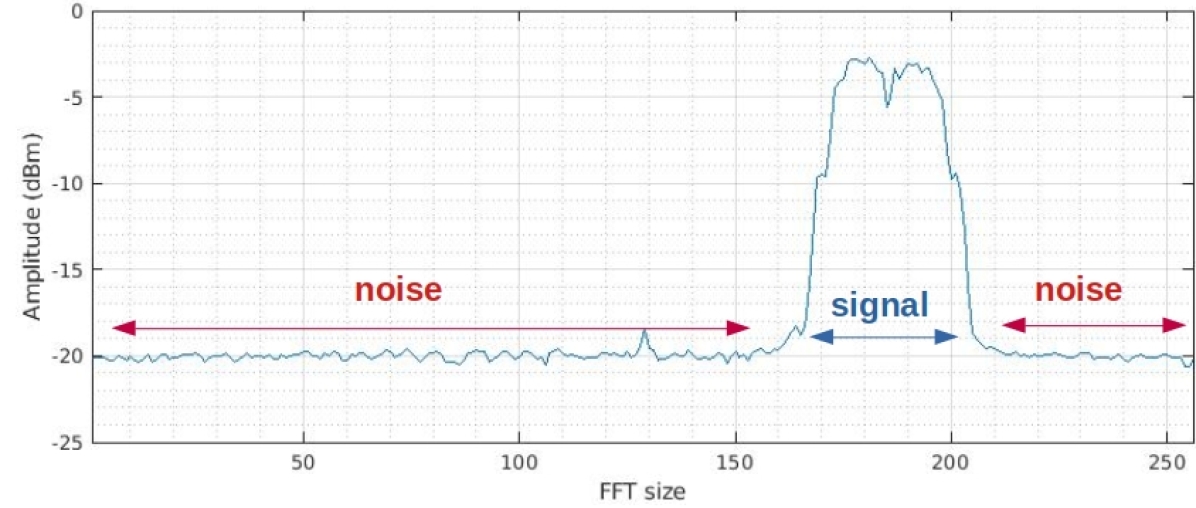
(a) SNR calculation in frequency domain

(b) Relation between noise vs SNR

Figure 4: SNR calculations of wideband signals

IV-C Implementation details

The classifier was implemented with Keras running on top of Tensorflow [23]. We performed the classification on a Intel core i7 computer with nvidia geforce RTX 2080 GPU. For the optimization, we used adam optimizer [24] with a learning rate of 0.001. In order to calculate the loss function while training, we used categorical crossentropy as the metric. The training was performed for 200 epochs with a batch size of 32.

V Results

V-A Classification under AWGN conditions

The classification accuracy under the AWGN conditions is plotted in Fig 5. We obtained a classification accuracy of nearly 100$\%$ with the introduced noise ranging from -60 to -40 dBm, which corresponds to the average signal SNR of 3 dB to -5 dB (Fig 4). The accuracy linearly decreases as the noise increases from -40 to 0 dBm. To visualize the classification accuracy of each class, we plotted the confusion matrix at -30 dB noise in Fig 6, where we obtained the classification accuracy of 87.6$\%$. At this SNR, we can observe some confusion in the classification between Tello and WiFi, since both use similar transmit signal. Apart from these two TXs, Q205 also shows lower classification accuracy and displays some confusion with Tello and WiFi. Although q205 does not transmit the same type of signal as Tello and WiFi, the transmit power was observed to be lower compared to the other transmitters. Therefore, with higher noise value the signal from q205 goes much inside noise compared to the other devices. Overall, the classifier provided good performance, it classified the drone signals even at lower SNR regions and distinguished the drone signals from the WiFi signal.

Figure 5: Classification accuracy under AWGN conditions. Train samples: 15k, Test samples: 4k

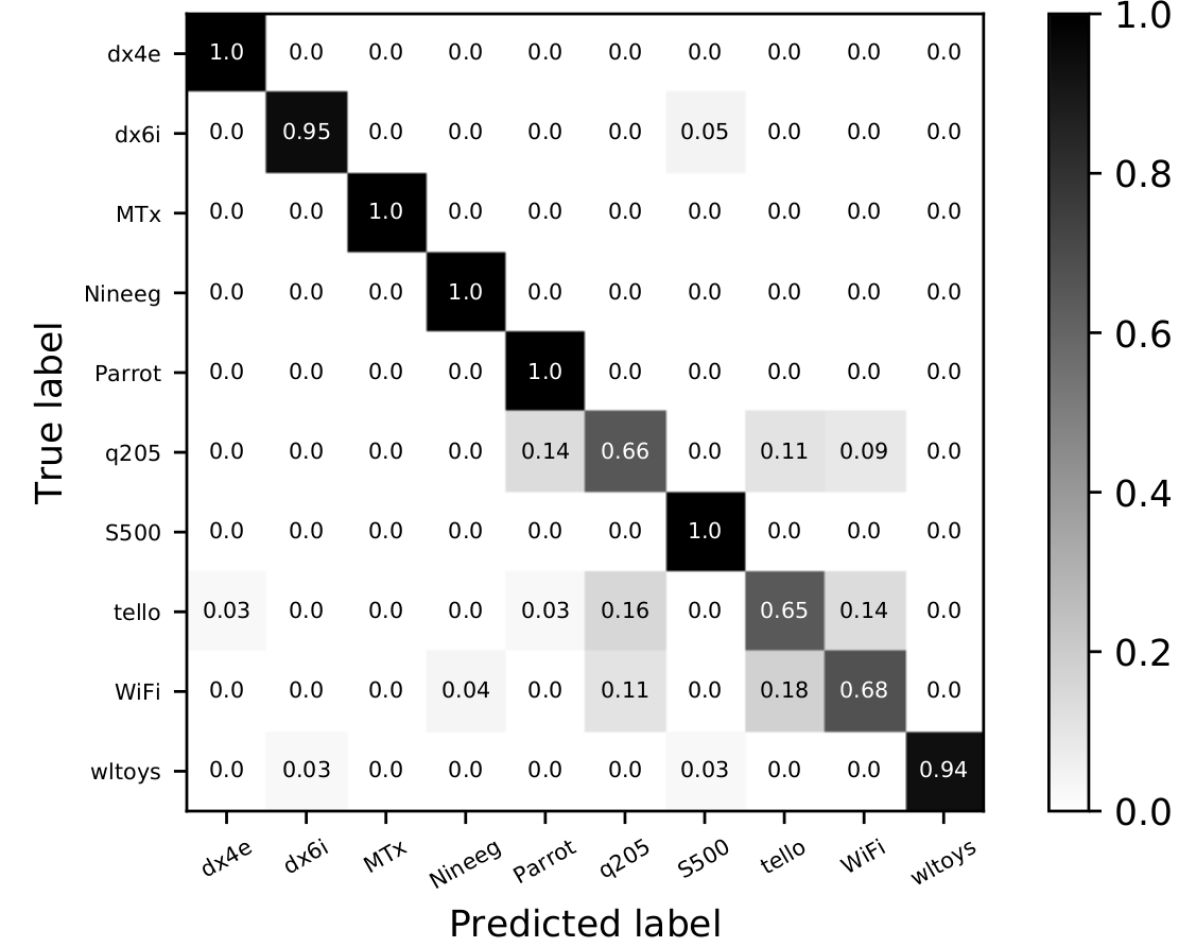
Figure 6: Confusion matrix with AWGN -30 dBm

V-B Effect of multipath environment

(a) Classification performance in Rician environment

(b) Classification performance in Rayleigh environment

Figure 7: Influence of multipath environment on classification performance. The classifier is trained with AWGN faded dataset and tested with Rician and Rayleigh faded dataset.

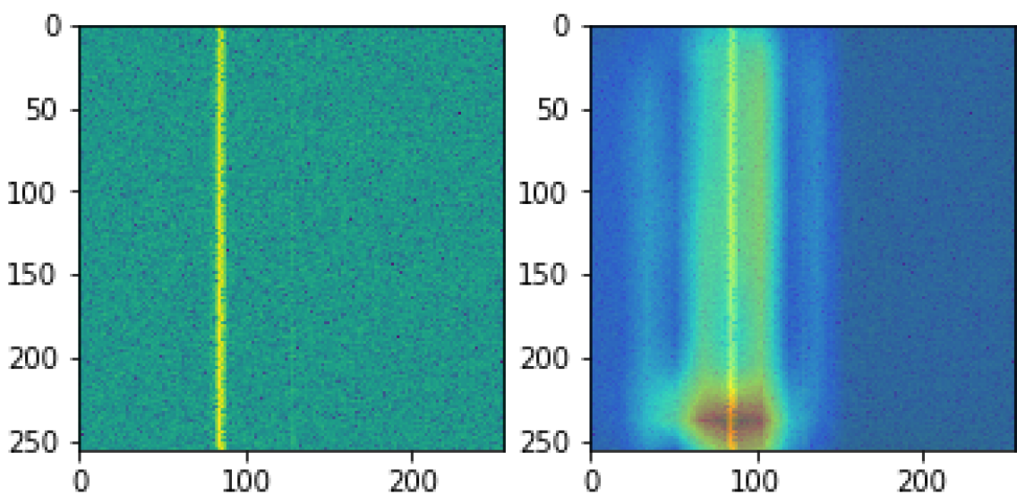
(a) DX4E

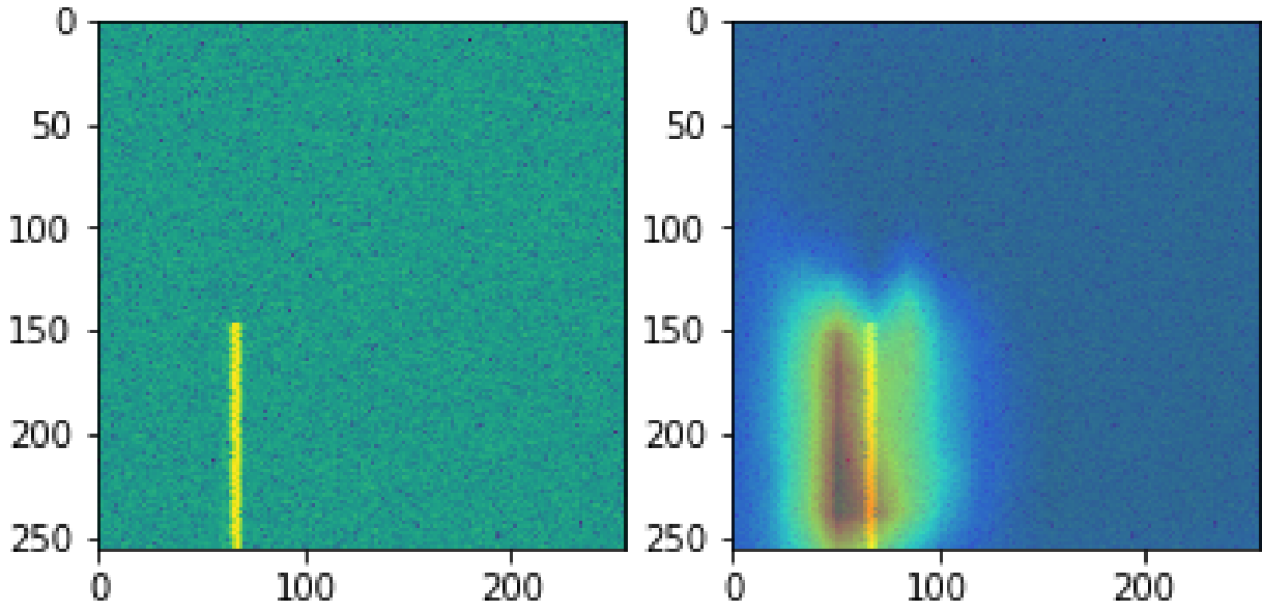
(b) DX6i

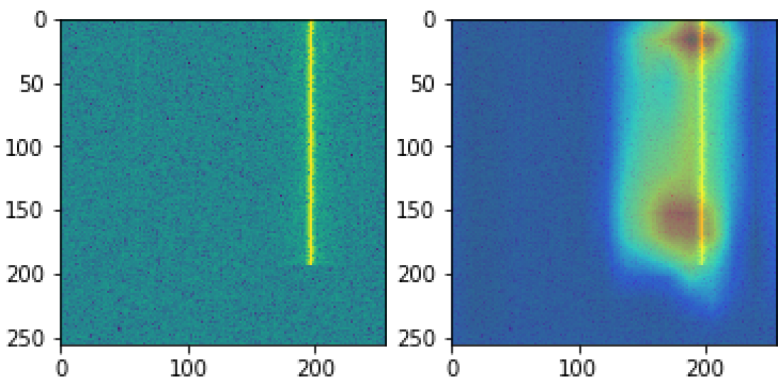
(c) MultiTx

(d) Nine Eagles

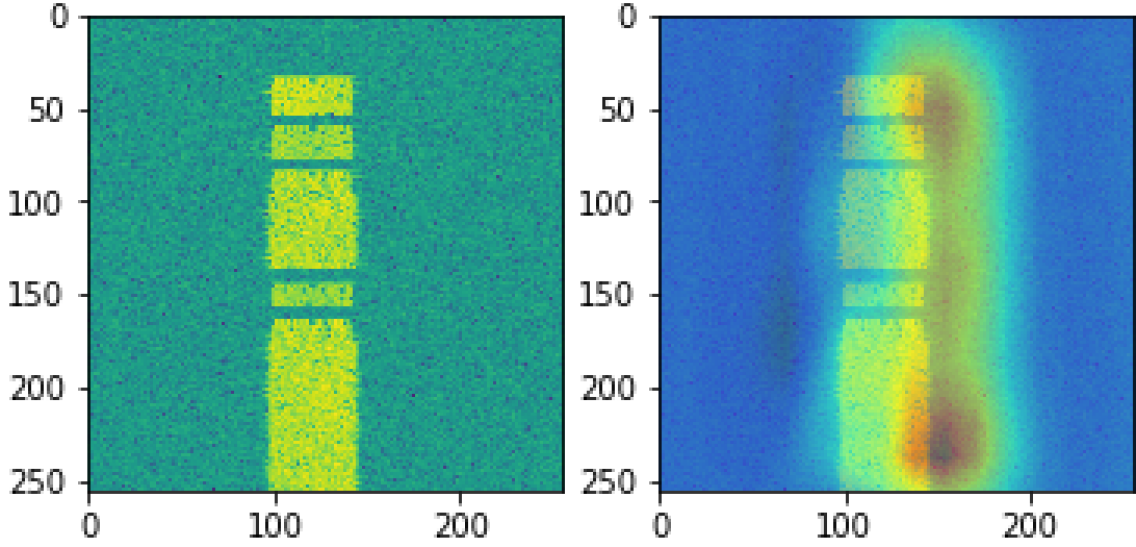
(e) Parrot

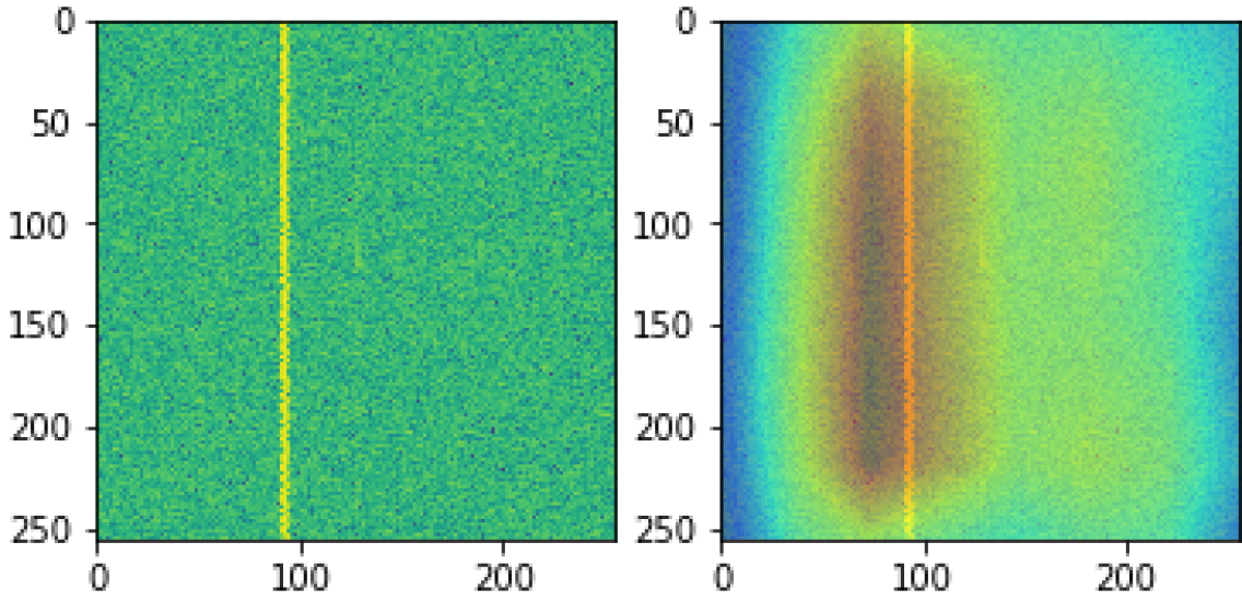
(f) Q205

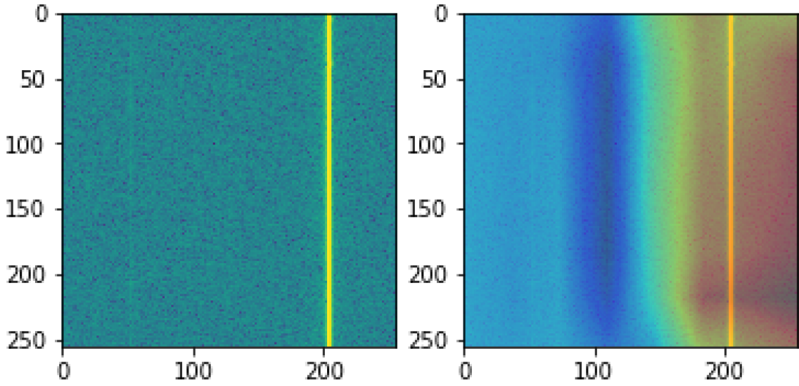
(g) S500 True

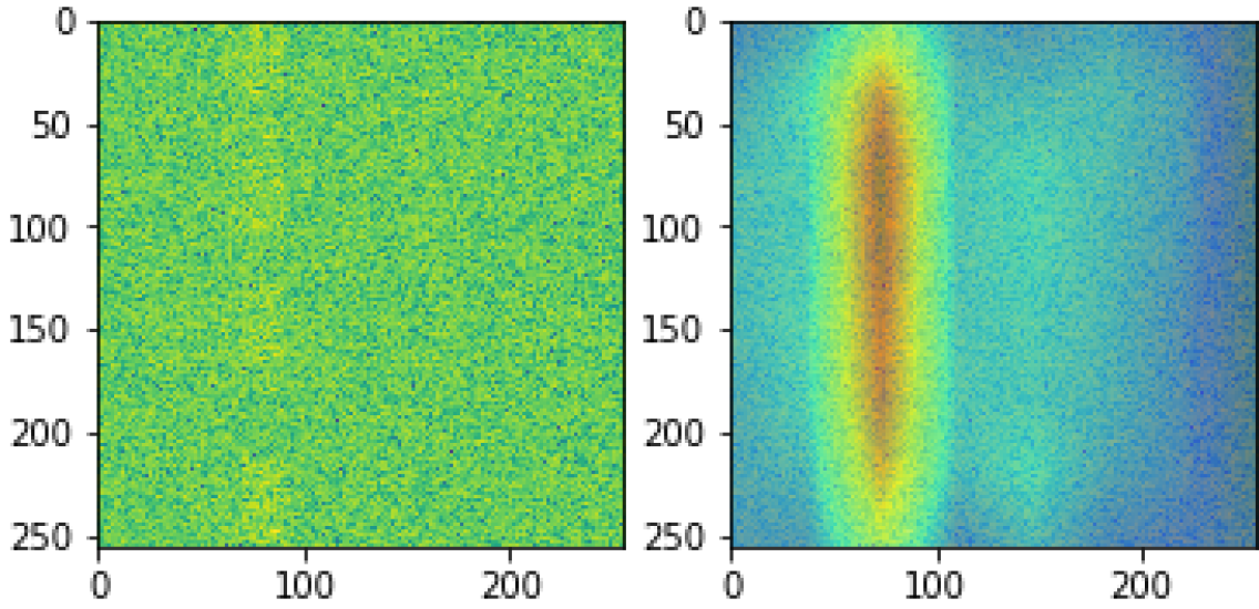
(h) Tello

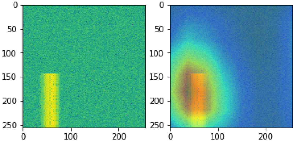
(i) WiFi

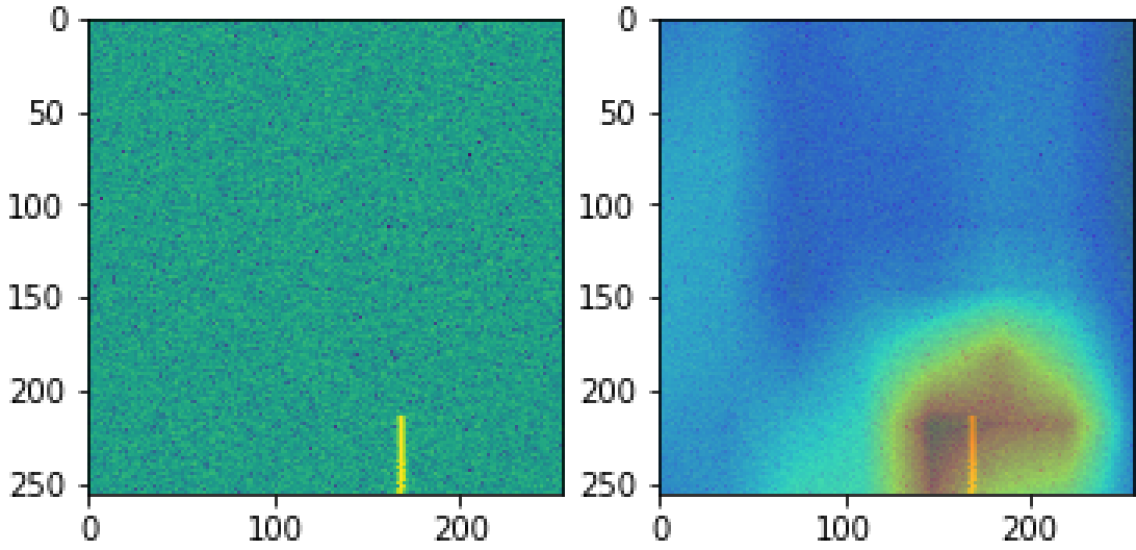
(j) wltoys

Figure 8: Class activation map for all signals under different AWGN conditions.

To understand the influence of channel variations on the classification performance, we tested the classifier with Multipath faded dataset, which was trained with AWGN conditions. In order to introduce multipath fading, we propagated the signals through a simulated Rician and Rayleigh channel. The following path delay and gain vector was used during the simulation:
path delay (sec) : [0, 200, 800]*$10^{-9}$
gain vector (dB) : [0, -3, -5]
K-factor: 2.8
We used Jakes Doppler spectrum for both Rician and Rayleigh channels. For the Rician channel, we used K-factor of 2.8 and the doppler for LOS path was kept the same as for multipath. Later, the signal SNR was varied and the performance was tested.

The classification performance in the Rician multipath channel is shown in Fig 7. We can see that the classification performance remained almost the same for the Doppler frequency ranging from 100 Hz to 100 kHz. Although at the higher SNR regions, a slight degradation of around 5-10 $\%$ in the classification accuracy can be observed, the classification performance remained the same for lower the SNR region. Significant drops in the classification accuracy were observed for very high Doppler frequencies like 500 kHz and 1 MHz. At 2.4 GHz, a Doppler frequency of 500 kHz corresponds to a velocity of 6.2457$\times$10⁴ m/s, which is practically not possible from a commercial drone.

The classification performance in the Rayleigh multipath channel is shown in Fig 7. The classifier also showed a good performance with the Rayleigh faded dataset for Doppler frequency ranging from 100 Hz to 10 kHz. The classification performance starts degrading from the Doppler frequency of 50 kHz. We can also clearly see that the classification performance is better with Rician faded dataset compared to the Rayleigh counterpart for higher Doppler frequencies. This is generally expected since for Rayleigh fading the multipath signals does not include the LOS component, the resultant signal suffers more fading.

Overall, the classifier performed equally well for both Rician and Rayleigh fading scenario for Doppler frequencies corresponding to a real drone’s velocity. The performance clearly explains the generalization capability of our classifier.

V-C Class Activation mapping

The activation maps of the drone and WiFi signals are shown in Fig 8. It provides an insight into what features the model is looking for while activating a particular class. The activation mapping can also be used as a tool for frequency localization in this case. It can be observed from the heatmap that the activation location corresponds to the frequency location of the signal. The model only learns the part of the spectrum which are important for classification. For example, for Nine Eagles (Fig 8), the model learns bottom and edges of the spectrum, whereas for MultiTx (Fig 8), the model learns the start and ending of the spectrum.

V-D Impact of residual mapping

The importance of residual mapping on the classification performance is investigated in this section. To perform the test, we have used 6 layered residual network with and without skip connection. The classification performance for two scenarios are shown in Fig 9. First, we trained and tested our models with a dataset on where the introduced AWGN was varied from -60 dB to 10 dB. The classification performance is shown in Fig 9 (left). The classifier without the skip connection could not learn from this noisy dataset, therefore, the performance remained poor throughout different SNR regions. However, the DRN model could learn features from the noisy dataset and the performance remained good throughout the SNR regions.

We created another training dataset with a less noisy signal, where the AWGN was varied from -60 dB to -15 dB. With this dataset, the classifier without skip connection could learn necessary features to classify the signal. The performance is shown in Fig 9 (right).

Figure 9: Classification performance with and without residual mapping

V-E Performance dependence on network depth

The classification performance generally improves with the increase in network depth. In this section, we show the dependency of the classification performance on the network depth. We varied the number of residual stacks (L) from 2 to 7 to visualize the impact of network depth on the classification performance. The average classification accuracy for different layers are plotted in Fig 10. We can see that the accuracy increases with the increase in network depth. However, we haven’t observed any improvement in classification performance after layer depth 6, the performance saturates after this layer depth.

Figure 10: Classification performance vs network depth

V-F Performance comparison with other machine learning models

The classification performance of our framework is compared with other machine learning algorithms like Support Vector Machines (SVM), Random Forest and Extreme Gradient Boosting (XGBoost) and the FC-DNN model proposed in [5]. The test is performed with the spectrogram dataset under AWGN conditions. For SVM, Random Forest and XGBoost, we have performed hyperparameter training using grid search. The classification performance for different frameworks is shown in Fig 11. Our DRNN model provided the best performance compared to other models. At high SNRs, SVM with a linear kernel and penalty factor (C=1) provided the same F1 score as the DRNN model. At lower SNRs, our DRNN model performed better than the SVM framework. At AWGN -30 dBm (i.e. -9.4 dB SNR), our classifier provided nearly 5$\%$ better F1 score and at -15 dBm (i.e. -15 dB SNR), it gave nearly 10$\%$ better F1 score compared to the SVM model. XGBoost with a max depth of 10 and random forest with 200 decision trees provided a lower F1-score compared the SVM and DRNN model. On the contrary, FC-DNN model showed a poor performance compared to all other frameworks. This clearly shows that a simple 3 layer FC-DNN model is not appropriate for classifying noisy spectrogram dataset.

Figure 11: Performance comparison between different models under AWGN conditions

V-G Simultaneous multidrone classification

In this section, we investigate the problem of simultaneous multiple drone classification. The simulation schematic of the dataset preparation is shown in Fig 12. We have added the signals on Matlab to have all different possible combinations and fed through an AWGN channel. One example is shown in Fig 12, where seven signals are present in the spectrogram dataset.

The classification performance for simultaneous multi-drone is shown in Fig 13. We have used 0.5 as the decision threshold. We can see that the classification performance is almost the same as with the single drone classification. We obtained F1 score ranging from 97.3 to 99.7 $\%$ for the introduced AWGN ranging from -40 to -50 dBm. We did not observe any significant decrease in the classification performance with the increase in the number of the source. On the contrary, an increase in classification performance can be observed with the increase in source numbers. Since within the dataset we mostly have narrowband signals and they are less impacted with high noise compared to the wideband signals, the combination of the signal showed better performance on average compared to the single drone scenario. The classification performance of each class remained almost the same for the simultaneous multi-class scenario as the singular counterpart. The result shows that our classifier does not only classify multiple drones simultaneously at lower SNR regions perfectly, it can also distinguish and classify the drone signals in the presence of WiFi communication.

(a) Simulation schematic

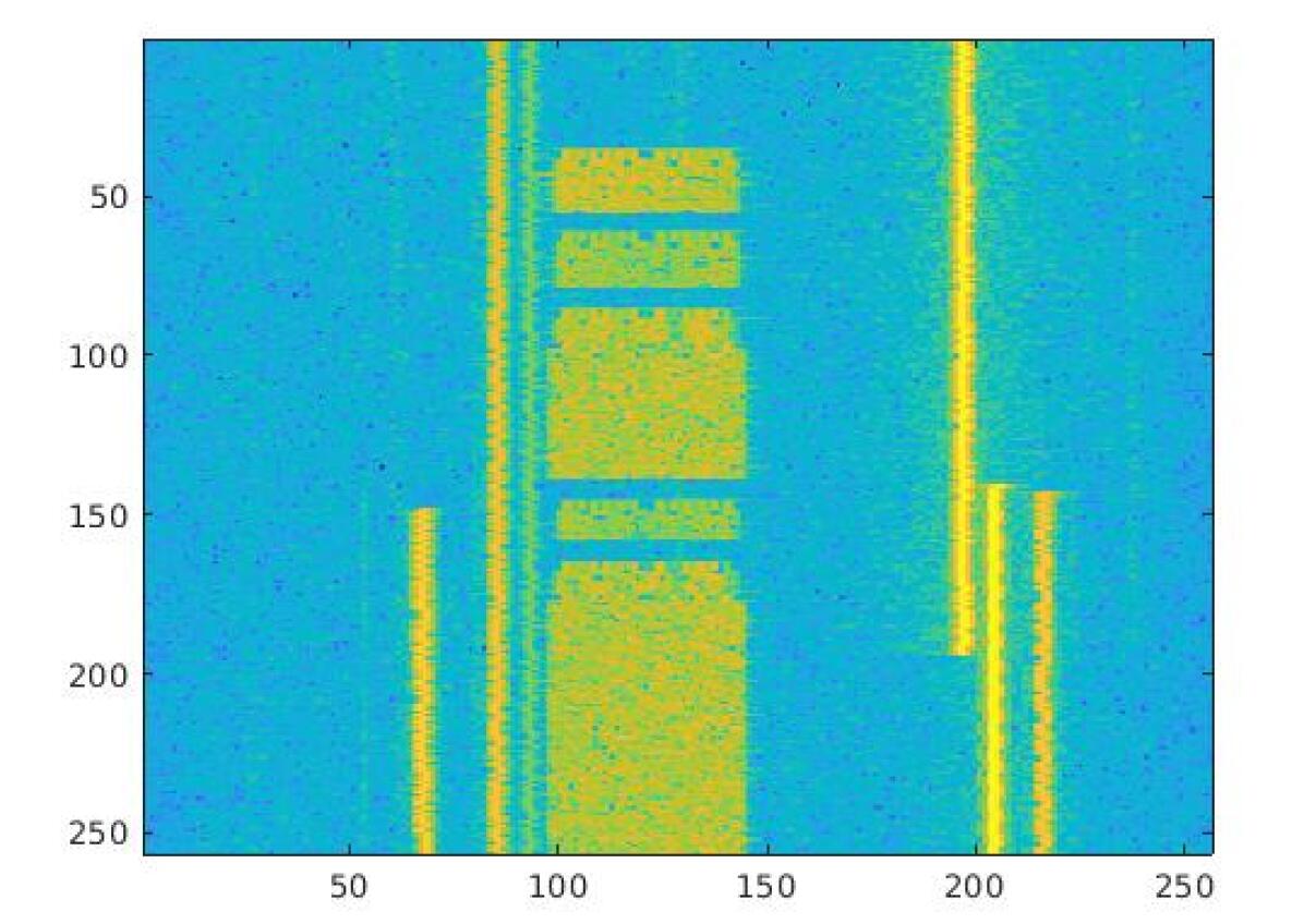
(b) Simultaneous presence of 7 signals

Figure 12: Simultaneous multiple signal classification experiment

Figure 13: Simultanous multi-drone classification performance under AWGN conditions

Conclusion

In this paper, we have proposed a deep residual network to classify several drone signals in a single drone and simultaneous multi-drone scenario. We have created a dataset using nine commercial drones and WiFi signals and evaluated the classification performance in AWGN and multipath environments. The importance of residual mapping and the dependence of the network depth on the classification performance is presented. Along with that, the class activation map is visualized. Furthermore, we have compared the classification performance of our model with other existing frameworks. Our proposed method outperformed the existing RF-based signal classification models and other standard wireless identification techniques by a good margin. At around 0 dB SNR, we achieved nearly 99$\%$ classification accuracy for both single and simultaneous multi-drone scenario. For the single drone scenario, our classifier provided around 5$\%$ better F1 score compared to the existing framework at -10 dB SNR. In the future work, we are going to investigate the classification performance in a frequency overlap scenario. Along with that, we are going to investigate combined RF signal detection, localization and classification using the latest computer vision methods and compare the performance with the two-stage detection and classification method.

References

- [1] A. Solodov, A. Williams, S. Hanaei, and B. Goddard, “Analyzing the threat of unmanned aerial vehicles (uav) to nuclear facilities,” Security Journal, 04 2017.
- [2] S. R. Ganti and Y. Kim, “Implementation of detection and tracking mechanism for small uas,” in 2016 International Conference on Unmanned Aircraft Systems (ICUAS), 2016, pp. 1254–1260.
- [3] P. Nguyen, M. Ravindranatha, A. Nguyen, R. Han, and T. Vu, “Investigating cost-effective rf-based detection of drones,” 06 2016, pp. 17–22.
- [4] P. Kosolyudhthasarn, V. Visoottiviseth, D. Fall, and S. Kashihara, “Drone detection and identification by using packet length signature,” in 2018 15th International Joint Conference on Computer Science and Software Engineering (JCSSE), 2018, pp. 1–6.
- [5] M. Al-Sa’d, A. Al-Ali, T. Khattab, and A. Erbad, “Rf-based drone detection and identification using deep learning approaches: An initiative towards a large open source drone database,” Future Generation Computer Systems, vol. 100, 05 2019.
- [6] T. Andre, K. A. Hummel, A. P. Schoellig, E. Yanmaz, M. Asadpour, C. Bettstetter, P. Grippa, H. Hellwagner, S. Sand, and S. Zhang, “Application-driven design of aerial communication networks,” IEEE Communications Magazine, vol. 52, no. 5, pp. 129–137, 2014.
- [7] J. Geier, “802.11 beacons revealed.” [Online]. Available: https://www.scribd.com/document/354688905/802-11-Beacons-Revealed
- [8] B. Scheers, D. Teguig, and V. Le Nir, “Wideband spectrum sensing technique based on goodness-of-fit testing,” in 2015 International Conference on Military Communications and Information Systems (ICMCIS), 2015, pp. 1–6.
- [9] S. Basak and B. Scheers, “Passive radio system for real-time drone detection and doa estimation,” in 2018 International Conference on Military Communications and Information Systems (ICMCIS), May 2018, pp. 1–6.
- [10] S. Rajendran, W. Meert, D. Giustiniano, V. Lenders, and S. Pollin, “Deep learning models for wireless signal classification with distributed low-cost spectrum sensors,” IEEE Transactions on Cognitive Communications and Networking, pp. 1–1, 2018.
- [11] T. J. O’Shea, T. Roy, and T. C. Clancy, “Over-the-air deep learning based radio signal classification,” IEEE Journal of Selected Topics in Signal Processing, vol. 12, no. 1, pp. 168–179, Feb 2018.
- [12] T. J. O’Shea and J. Corgan, “Convolutional radio modulation recognition networks,” CoRR, vol. abs/1602.04105, 2016. [Online]. Available: http://arxiv.org/abs/1602.04105
- [13] E. Perenda, S. Rajendran, and S. Polin, “Automatic modulation classification using parallel fusion of convolutional neural networks,” 06 2019.
- [14] N. T. Nguyen, G. Zheng, Z. Han, and R. Zheng, “Device fingerprinting to enhance wireless security using nonparametric bayesian method,” in 2011 Proceedings IEEE INFOCOM, 2011, pp. 1404–1412.
- [15] A. Krizhevsky, I. Sutskever, and G. Hinton, “Imagenet classification with deep convolutional neural networks,” Neural Information Processing Systems, vol. 25, 01 2012.
- [16] O. Abdel-Hamid, A. Mohamed, H. Jiang, L. Deng, G. Penn, and D. Yu, “Convolutional neural networks for speech recognition,” IEEE/ACM Transactions on Audio, Speech, and Language Processing, vol. 22, no. 10, pp. 1533–1545, 2014.
- [17] S. Riyaz, K. Sankhe, S. Ioannidis, and K. Chowdhury, “Deep learning convolutional neural networks for radio identification,” IEEE Communications Magazine, vol. 56, no. 9, pp. 146–152, Sep. 2018.
- [18] Y. Bengio, P. Simard, and P. Frasconi, “Learning long-term dependencies with gradient descent is difficult,” IEEE Transactions on Neural Networks, vol. 5, no. 2, pp. 157–166, March 1994.
- [19] X. Glorot and Y. Bengio, “Understanding the difficulty of training deep feedforward neural networks,” Journal of Machine Learning Research - Proceedings Track, vol. 9, pp. 249–256, 01 2010.
- [20] S. Ioffe and C. Szegedy, “Batch normalization: Accelerating deep network training by reducing internal covariate shift,” 2015.
- [21] K. He, X. Zhang, S. Ren, and J. Sun, “Deep residual learning for image recognition,” CoRR, vol. abs/1512.03385, 2015. [Online]. Available: http://arxiv.org/abs/1512.03385
- [22] B. Zhou, A. Khosla, ‘A. gata Lapedriza, A. Oliva, and A. Torralba, “Learning deep features for discriminative localization,” CoRR, vol. abs / 1512.04150, 2015. [Online]. Available: http://arxiv.org/abs/1512.04150
- [23] Keras documentation. [Online]. Available: http://keras.io/
- [24] D. P. Kingma and J. Ba, “Adam: A method for stochastic optimization,” 2014.