Third order corrections to the semi-leptonic $b\to c$ and the muon decays

Abstract

We compute corrections of order $\alpha_{s}^{3}$ to the decay $b\to c\ell\bar{\nu}$ taking into account massive charm quarks. In the on-shell scheme large three-loop corrections are found. However, in the kinetic scheme the three-loop corrections are below 1% and thus perturbation theory is well under control. We furthermore provide results for the order $\alpha_{s}^{3}$ corrections to $b\to u\ell\bar{\nu}$ and the third-order QED corrections to the muon decay which will be important input for reducing the uncertainty of the Fermi coupling constant $G_{F}$.

I Introduction

The Cabibbo-Kobayashi-Maskawa (CKM) matrix determines the mixing strength in the quark sector and provides furthermore the source for charge-parity (CP) violation in the Standard Model (SM). It is thus of prime importance to determine the parameters of the CKM matrix with highest accuracy. In this article we address the elements $V_{ub}$ and $V_{cb}$ which are accessible via semi-leptonic $B$ meson decays.

At present, the value of $|V_{cb}|$ from inclusive $B\to X_{c}\ell\bar{\nu}$ decays is obtained from global fits Gambino:2013rza ; Alberti:2014yda ; Gambino:2016jkc . The experimental inputs are the semileptonic width and the moments of kinematical distributions measured at Belle Urquijo:2006wd ; Schwanda:2006nf and BABAR Aubert:2004td ; Aubert:2009qda , together with earlier data from CDF Acosta:2005qh , CLEO Csorna:2004kp and DELPHI Abdallah:2005cx . The most recent determination in the so-called kinetic scheme $|V_{cb}|=(42.19\pm 0.78)\times 10^{-3}$ Amhis:2019ckw has a relative error of about 1.8%, which is mostly dominated by theoretical uncertainties. Global fits in the 1S scheme yield $|V_{cb}^{\mathrm{1S}}|=(41.98\pm 0.45)\times 10^{-3}$ Bauer:2004ve ; Amhis:2019ckw .

A crucial ingredient for the determination of $|V_{ub}|$ and $|V_{cb}|$ is the total semi-leptonic decay rate. Branching ratios of inclusive semileptonic $B$ mesons were measured at $B$ factories with a relative precision of about 2.5% TheBABAR:2016lja ; Urquijo:2006wd ; Mahmood:2004kq ; Albrecht:1993pu . A relative uncertainty of 1.5% is obtained with the help of a global fit: $\mathrm{Br}(B\to X_{c}\ell^{+}\nu_{\ell})=(10.65\pm 0.16)\%$ Amhis:2019ckw . Measurements are performed with a mild lower cut on the electron energy Urquijo:2006wd , which excludes less than 5% of the events, or extrapolated to the whole phase space based on Monte Carlo TheBABAR:2016lja ; Mahmood:2004kq . A key goal for Belle II is the reduction of the systematic uncertainties on the branching fraction determinations, as well as to obtain more precise and detailed measurements of $B\to X_{c}\ell\bar{\nu}_{\ell}$ differential distributions Kou:2018nap . Recent analyses by Belle and Belle II of leptonic and hadronic invariant mass moments q2moments ; Abudinen:2020zwm show that a percent or even sub-percent relative accuracy can be achieved for certain observables.

With the help of the heavy quark expansion it can be written as a double series in $\alpha_{s}$ and $\Lambda_{\rm QCD}/m_{b}$. The $m_{b}$-suppressed corrections are obtained from higher-dimensional operators. In the free-quark approximation, corrections up to ${\cal O}(\alpha_{s}^{2})$ are available Luke:1994yc ; Trott:2004xc ; Aquila:2005hq ; Pak:2008qt ; Pak:2008cp ; Melnikov:2008qs ; Biswas:2009rb ; Gambino:2011cq ; Dowling:2008mc together with the leading $\beta_{0}$ terms at higher orders Ball:1995wa , where $\beta_{0}$ is the one-loop coefficient of the QCD beta function. The power corrections of order $\Lambda_{\mathrm{QCD}}^{2}/m_{b}^{2}$ and $\Lambda_{\mathrm{QCD}}^{3}/m_{b}^{3}$ have been computed in Chay:1990da ; Bigi:1993fe ; Manohar:1993qn ; Gremm:1996df to tree-level and in Becher:2007tk ; Alberti:2013kxa ; Mannel:2014xza ; Mannel:2019qel to ${\cal O}(\alpha_{s})$. Also $1/m_{b}^{4}$ and $1/m_{b}^{5}$ terms are known, however, only at leading order Dassinger:2006md ; Mannel:2010wj ; Mannel:2018mqv ; Fael:2018vsp . Note that linear $1/m_{b}$ corrections vanish to all orders. Missing higher-order perturbative and power corrections limit the current extraction of $|V_{cb}|$.

The relative size of the second order corrections to the partonic $b\to c\ell\bar{\nu}_{\ell}$ decays is about $1-3\%$ depending on the quark mass scheme, with a theoretical uncertainty due to renormalization scale variation estimated to be 1% Gambino:2011cq , which soon can become comparable to experimental errors. In this work we make a major improvement in the theory underlying $B\to X_{c}\ell\bar{\nu}$ decays by computing the $\alpha_{s}^{3}$ corrections to the total rate, at leading order in $1/m_{b}$. We incorporate a finite charm quark mass via an expansion in the mass difference $m_{b}-m_{c}$ and show that precise results can be obtained for the physical values of $m_{c}$ and $m_{b}$. Our analysis even allows for the limit $m_{c}\to 0$ which provides $\alpha_{s}^{3}$ corrections for the decay rate $\Gamma(B\to X_{u}\ell\bar{\nu})$.

A process closely related to $b\to u\ell\bar{\nu}$ is the muon decay. Its lifetime, $\tau_{\mu}$, can be written in the following form

$$\frac{1}{\tau_{\mu}} \equiv \Gamma(\mu^{-}\to e^{-}\nu_{\mu}\bar{\nu}_{e})=\frac{G_{F}^{2}m_{\mu}^{5}}{192\pi^{3}}\left(1+\Delta q\right)\,,$$ (1)

where $G_{F}$ is the Fermi constant, $m_{\mu}$ is the muon mass and $\Delta q$ contains QED and hadronic vacuum polarization corrections (see Ref. Kinoshita:1958ru ; vanRitbergen:1999fi ; Ferroglia:1999tg for details). Note that all weak corrections are absorbed in $G_{F}$. Equation (1) allows for the determination of $G_{F}$ if precise measurements of $\tau_{\mu}$ are combined with accurate QED predictions. We compute for the first time $\alpha^{3}$ corrections to $\Delta q$ by specifying the colour factors of our $b\to c\ell\bar{\nu}$ result to QED and taking the limit $m_{c}\to 0$. This allows for the determination of the third-order coefficient with an accuracy of 15%.

II Calculation

We apply the optical theorem and consider the forward scattering amplitude of a bottom quark where at leading order the two-loop diagram in Fig. 1(a) has to be considered. It has a neutrino, a lepton and a charm quark as internal particles. The weak interaction is shown as an effective vertex. Our aim is to consider QCD corrections up to third order which adds up to three more loops. Some sample Feynman diagrams are shown in Fig. 1(b-f).

(a) (b) (c) (d) (e) (f)

Figure 1: Sample Feynman diagrams which contribute to the forward scattering amplitude of a bottom quark at LO (a), NLO (b), NNLO (c) and N³LO (d-f). Straight, curly and dashed lines represent quarks, gluons and leptons, respectively. The weak interaction mediated by the $W$ boson is shown as a blob.

The structure of the Feynman diagrams allows the integration of the massless neutrino-lepton loop which essentially leads to an effective propagator raised to an $\epsilon$-dependent power, where $d=4-2\epsilon$ is the space-time dimension. The remaining diagram is at most of four-loop order.

From the technical point of view there are two basic ingredients which are crucial to realize our calculation. First, we perform an expansion in the difference between the bottom and charm quark mass. It has been shown in Ref. Dowling:2008mc that the expansion converges quite fast for the physical values of $m_{c}$ and $m_{b}$. Second, we apply the so-called method of regions Beneke:1997zp ; Smirnov:2012gma and exploit the similarities to the calculation of the three-loop corrections to the kinetic mass Fael:2020iea .

The method of regions Beneke:1997zp ; Smirnov:2012gma leads to two possible scalings for each loop momentum $k^{\mu}$

• $|k^{\mu}|\sim m_{b}$ ($h$, hard)

• $|k^{\mu}|\sim\delta\cdot m_{b}$ ($u$, ultra-soft)

with $\delta=1-m_{c}/m_{b}$. We choose the notion “ultra-soft” for the second scaling to stress the analogy to the calculation of the relation between the pole and the kinetic mass of a heavy quark, see Fael:2020iea ; FSS-mkin-long . Note that the momentum which flows through the neutrino-lepton loop, $\ell$, has to be ultra-soft since the Feynman diagram has no imaginary part if $\ell$ is hard since the corresponding on-shell integral has no cut.

Let us next consider the remaining (up to three) momentum integrations which can be interpreted as a four-point amplitude with forward-scattering kinematics and two external momenta: $\ell$ and the on-shell momentum $p^{2}=m_{b}^{2}$. This is in close analogy to the scattering amplitude of a heavy quark and an external current considered in Ref. Fael:2020iea . In fact, at each loop order each momentum can either scale as hard or ultra-soft:
${\cal O}(\alpha_{s})$ $h,u$ ${\cal O}(\alpha_{s}^{2})$ $hh,hu,uu$ ${\cal O}(\alpha_{s}^{3})$ $hhh,hhu,huu,uuu$
Note that all regions where at least one of the loop momenta scales ultra-soft leads to the same integral families as in Ref. Fael:2020iea ; FSS-mkin-long . The pure-hard regions were absent in Fael:2020iea ; FSS-mkin-long ; they lead to (massive) on-shell integrals.

At this point there is the crucial observation that the integrands in the hard regions do not depend on the loop momentum $\ell$. On the other hand, the ultra-soft integrals still depend on $\ell$. However, for each individual integral the dependence of the final result on $\ell$ is of the form

$$(-2p\cdot\ell+2\delta)^{\alpha}$$ (2)

with known exponent $\alpha$. This means that it is always possible to perform in a first step the $\ell$ integration which is of the form

$$\int{\rm d}^{d}\ell\frac{\ell^{\mu_{1}}\ell^{\mu_{2}}\cdots}{(-2p\cdot\ell+2\delta)^{\alpha}(-\ell^{2})^{\beta}}\,.$$ (3)

A closed formula for such tensor integrals with arbitrary tensor rank and arbitrary exponents $\alpha$ and $\beta$ can easily be obtained from the formula provided in Appendix A of Ref. Smirnov:2012gma . We thus remain with the loop integrations given in the above table. Similar to Eq. (3) we can integrate all one-loop hard or ultra-soft loops which leaves us with pure hard or pure ultra-soft contributions up to three loops.

A particular challenge of our calculation is the high expansion depth in $\delta$. We perform an expansion of all diagrams up to $\delta^{12}$. This leads to huge intermediate expressions of the order of 100 GB. Furthermore, for some of the scalar integrals individual propagators are raised to positive and negative powers up to 12, which is a non-trivial task for the reduction to master integrals. For the latter we combine FIRE Smirnov:2019qkx and LiteRed Lee:2012cn . For the subset of integrals which are needed for the expansion up to $\delta^{10}$ we also use the stand-alone version of LiteRed Lee:2012cn as a cross-check. For all regions where at least one of the regions is ultra-soft we can take over the master integrals from Fael:2020iea ; FSS-mkin-long . For some of the (complicated) three-loop triple-ultra-soft master integrals higher order $\epsilon$ terms are needed. The method used for their calculation and the results are given Ref. FSS-mkin-long . All triple-hard master integrals can be found in Ref. Lee:2010ik .

III Results

We write the total decay rate for the $b\to c$ transition in the form

$$\Gamma(B\to X_{c}\ell\bar{\nu}) = \Gamma_{0}\left[X_{0}+C_{F}\sum_{n\geq 1}\left(\frac{\alpha_{s}}{\pi}\right)^{n}X_{n}\right]$$ (4)

$$+{\cal O}\left(\frac{\Lambda_{\rm QCD}^{2}}{m_{b}^{2}}\right)\,,$$

with $C_{F}=4/3$, $\Gamma_{0}=A_{\rm ew}G_{F}^{2}|V_{cb}|^{2}m_{b}^{5}/(192\pi^{3})$, $X_{0}=1-8\rho^{2}-12\rho^{4}\log(\rho^{2})+8\rho^{6}-\rho^{8}$ where $\rho=m_{c}^{\rm OS}/m_{b}^{\rm OS}$ and $\alpha_{s}\equiv\alpha_{s}^{(5)}(\mu_{s})$ with $\mu_{s}$ being the renormalization scale. $A_{\rm ew}=1.014$ is the leading electroweak correction Sirlin:1981ie and $m_{b}^{\rm OS}$ ($m_{c}^{\rm OS}$) is the bottom (charm) pole mass. The one- and two-loop results are available from Refs. Trott:2004xc ; Aquila:2005hq ; Pak:2008qt ; Pak:2008cp ; Melnikov:2008qs ; Biswas:2009rb ; Gambino:2011cq ; Dowling:2008mc . The main result of our calculation is $X_{3}$. In the following we set all colour factors to their numerical values. Furthermore, we specify the number of massless quarks to 3 and take into account closed charm and bottom loops. For $\mu=m_{b}$ we have

$$X_{3} = \sum_{n\geq 5}x_{3,n}\delta^{n}\,,$$ (5)

with analytic coefficients $x_{3,n}$, which in general depend on $\log(\delta)$. For illustration purposes we show explicit results only for the leading term which for dimensional reasons is of order $\delta^{5}$. Our result reads

$$C_{F}x_{3,5}=\frac{533858}{1215}-\frac{20992a_{4}}{81}+\frac{8744\pi^{2}\zeta_{3}}{135}-\frac{6176\zeta_{5}}{27}$$

$$-\frac{16376\zeta_{3}}{135}-\frac{2624l_{2}^{4}}{243}+\frac{5344\pi^{2}l_{2}^{2}}{1215}+\frac{179552\pi^{2}l_{2}}{405}$$

$$-\frac{39776\pi^{4}}{6075}-\frac{1216402\pi^{2}}{3645}\,,$$ (6)

where $l_{2}=\log(2)$, $a_{4}=\mbox{Li}_{4}(1/2)$ and $\zeta_{n}$ is the Riemann zeta function. Analytic results up to $\delta^{12}$ can be found in progdata . We note that the leading term given in Eq. (6) can be cross-checked against the results from Archambault:2004zs where the $b\to c$ transition has been computed in the limit $m_{c}=m_{b}$.

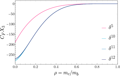
Figure 2: The third-order coefficient (see Eq. (4)) as a function of $\rho=m_{c}^{\rm OS}/m_{b}^{\rm OS}$ for different expansion depth in $\delta$.

In Fig. 2 we show $X_{3}$ as a function of $\rho=1-\delta=m_{c}^{\rm OS}/m_{b}^{\rm OS}$ where the different curves contain different expansion depths in $\delta$. One observes a rapid convergence at the physical point for the $b\to c$ decay which amounts to $\rho\approx 0.3$. In particular, the curves including terms up to $\delta^{10}$, $\delta^{11}$ or $\delta^{12}$ are basically indistinguishable for $\rho\approx 0.3$ which leads to $X_{3}(\rho=0.28)=-{68.4\pm 0.3}$, where the uncertainty is obtained from the difference of the $\delta^{11}$ and $\delta^{12}$ expansion, multiplied by a security factor of five.

	$Y_{1}$	$Y_{2}^{\rm rem}$	$\beta_{0}Y_{2}^{\beta_{0}}$	$Y_{3}^{\rm rem}$	$\beta_{0}^{2}Y_{3}^{\beta_{0}^{2}}$
$m_{b}^{\rm OS},m_{c}^{\rm OS}$	$-1.72$	$3.08$	$-16.17$	$48.8$	$-212.1$
$m_{b}^{\rm kin},m_{c}^{\rm kin}$	$-0.94$	$0.33$	$-4.08$	$-5.4$	$-15.4$
$m_{b}^{\rm kin},\overline{m}_{c}(3~{}\mbox{GeV})$	$-1.67$	$-3.39$	$-3.85$	$-97.7$	$69.1$
$m_{b}^{\rm kin},\overline{m}_{c}(2~{}\mbox{GeV})$	$-1.25$	$-1.21$	$-2.43$	$-68.8$	$67.9$
$\overline{m}_{b}(\overline{m}_{b}),\overline{m}_{c}(3~{}\mbox{GeV})$	$3.07$	$-21.81$	$35.17$	$-56.7$	$119.4$
$m_{b}^{\rm PS},\overline{m}_{c}(2~{}\mbox{GeV})$	$-0.47$	$-6.10$	$-2.31$	$-93.1$	$-7.19$
$m_{b}^{\rm 1S},\overline{m}_{c}(m_{b}^{\rm 1S})$	$-3.59$	$-0.98$	$-19.39$	$-39.83$	$-80.22$
$m_{b}^{\rm 1S},m_{c}$ via HQET	$-1.38$	$0.73$	$-7.05$	$5.04$	$-38.09$

Table 1: Numerical results for the coefficients $Y_{n}$ in Eq. (7) for various renormalization schemes.

For the numerical evaluation it is convenient to cast Eq. (4) in the form

$$\Gamma(B\to X_{c}\ell\bar{\nu}) = \Gamma_{0}X_{0}\left[1+\sum_{n\geq 1}\left(\frac{\alpha_{s}}{\pi}\right)^{n}Y_{n}\right]$$ (7)

$$\mbox{}+{\cal O}\left(\frac{\Lambda_{\rm QCD}^{2}}{m_{b}^{2}}\right)\,,$$

with $\alpha_{s}\equiv\alpha_{s}^{(4)}(\mu_{s})$ as expansion parameter. In the following we discuss various renormalization schemes for the charm and bottom quark masses, where $\Gamma_{0}$ and $X_{0}$ are evaluated using the respective numerical values. In Tab. 1 we provide the corresponding results for the coefficients $Y_{n}$. At two and three-loop orders we split the results into the large-$\beta_{0}$ contribution and the remaining term

$$Y_{2} = Y_{2}^{\rm rem}+\beta_{0}Y_{2}^{\beta_{0}}\,,$$

$$Y_{3} = Y_{3}^{\rm rem}+\beta_{0}^{2}Y_{3}^{\beta_{0}^{2}}\,,$$ (8)

with $\beta_{0}=11-2/3n_{l}=9$ where $n_{l}=3$ is the number of massless quarks. Note that the uncertainty of $Y_{3}$ due to the expansion in $\delta$ is of the same order of magnitude as for $X_{3}$ discussed above.

For the transition of the on-shell quark masses to the $\overline{\rm MS}$ scheme we use the three-loop formulae provided in Refs. Chetyrkin:1999qi ; Melnikov:2000qh . Finite-$m_{c}$ effects in the bottom mass relation are taken from Refs. Fael:2020bgs . The two- and three-loop corrections to the transition from the on-shell to the kinetic scheme are provided in Czarnecki:1997sz and Fael:2020iea ; FSS-mkin-long , respectively. Note that the transition to the kinetic scheme also requires the renormalization of the parameters $\mu_{\pi}^{2}$ and and $\rho_{D}^{3}$, which enter the decay rate at order $1/m_{b}^{2}$ and $1/m_{b}^{3}$, respectively. They receive additive contributions, which enter $Y_{i}$ in Eq. (7) Benson:2003kp ; Gambino:2007rp . The corresponding corrections up to three-loop order can be found in FSS-mkin-long . Note that we assume a heavy charm quark and thus we have $(n_{l}=3)$-flavour QCD as starting point for the on-shell–kinetic relations. We use the decoupling relation for $\alpha_{s}$ up to two-loop order to obtain expressions parameterized in terms of $\alpha_{s}^{(4)}$. For the decoupling scale we use $\mu_{s}$. It has been shown in Ref. FSS-mkin-long that there are no additional charm quark mass effects in the kinetic-on-shell relation. For comparison we show in Tab. 1 also results where the bottom quark mass is renormalized in the PS Beneke:1998rk and 1S Hoang:1998hm ; Hoang:1998ng ; Hoang:1999zc scheme. In the latter case we renormalize the charm quark mass both in the $\overline{\rm MS}$ and via the Heavy Quark Effective Theory (HQET) relation to on-shell bottom quark mass and (averaged) $D$ and $B$ meson masses (see, e.g., Ref. Hoang:1998ng ). After each scheme change we re-expand in $\alpha_{s}$ to third order.

Note that our two-loop results for $Y_{2}^{\rm rem}$ differ from the one of Ref. Alberti:2014yda due to finite charm quark mass effects in the relation between the kinetic and on-shell bottom quark mass and the renormalization of $\mu_{\pi}^{2}$ and $\rho_{D}^{3}$ FSS-mkin-long . This leads to a shift of about $-0.5$% in the leading $1/m_{b}$ approximation of the decay rate and thus might have a visible effect on the value of $|V_{cb}|$.

For the numerical evaluation of the decay rate we use the input values $m_{b}^{\rm OS}=4.7$ GeV, $m_{c}^{\rm OS}=1.3$ GeV, $m_{b}^{\rm kin}=4.526$ GeV, $m_{b}^{\rm PS}=4.479$ GeV, $m_{b}^{\rm 1S}=4.666$ GeV, $m_{c}^{\rm kin}=1.130$ GeV, $\overline{m}_{b}(\overline{m}_{b})=4.163$ GeV, $\overline{m}_{c}(3~{}\mbox{GeV})=0.993$ GeV, $\overline{m}_{c}(2~{}\mbox{GeV})=1.099$ GeV, and $\alpha_{s}^{(5)}(M_{Z})=0.1179$. We use RunDec Herren:2017osy for the running of the $\overline{\rm MS}$ parameters and the decoupling of heavy particles. For the Wilsonian cutoff in the kinetic scheme we use $\mu=1$ GeV both for the bottom and charm quark. In the case of PS scheme we use $\mu=2$ GeV. For the renormalization scale of $\alpha_{s}^{(4)}$, $\mu_{s}$, we choose the respective value for the bottom quark mass.

For illustration purpose we provide in Tab. 1 also results where both masses are defined in the on-shell scheme. It is well known that in this scheme the perturbative series shows a bad convergence behaviour. In fact, we have $Y_{3}\approx-163$ whereas in the schemes where the bottom quark mass is used in the kinetic scheme we have that $Y_{3}$ is between $-1$ and $-29$. Note, that in the scheme where both quark masses are defined in the $\overline{\rm MS}$ scheme the three-loop corrections are more than twice as big which also hints for a worse convergence behaviour. The PS and 1S schemes show a clear improvement as compared to the on-shell scheme. However, the convergence properties are significant worse than in the kinectic scheme in case the charm quark mass is renormalized in the $\overline{\rm MS}$ scheme. In case $m_{c}^{\rm OS}$ is expressed through $m_{b}^{\rm OS}$ and meson masses using a HQET relation one observes an improved perturbative behaviour. Still, the analysis clearly shows the advantage of the kinetic scheme which is constructed such that large corrections are resummed into the quark mass value. In fact, all three schemes which involve $m_{b}^{\rm kin}$ demonstrate a good convergence behaviour. Using $\alpha_{s}^{(4)}(m_{b}^{\rm kin})=0.2186$ we obtain for $\Gamma(B\to X_{c}\ell\bar{\nu})/\Gamma_{0}$ in these three schemes

$$m_{b}^{\rm kin},m_{c}^{\rm kin}: 0.633\left(1-0.066-0.018-0.007\right)$$

$$\approx 0.575\,,$$

$$m_{b}^{\rm kin},\overline{m}_{c}(3~{}\mbox{GeV}): 0.700\left(1-0.116-0.035-0.010\right)$$

$$\approx 0.587\,,$$

$$m_{b}^{\rm kin},\overline{m}_{c}(2~{}\mbox{GeV}): 0.648\left(1-0.087-0.018-0.0003\right)$$ (9)

$$\approx 0.580\,,$$

where the different $\alpha_{s}$ orders are displayed separately. Note that in the PS and 1S schemes the third-order corrections amount to 3.4% and 3.9%, respectively, with $m_{c}$ in the $\overline{\rm MS}$ scheme. If one defines $m_{c}$ in the 1S scheme via a HQET relation the third-order corrections reduce to 1%. For the bottom mass expressed in the kinetic scheme we observe that the third-order corrections amount to at most 1% and they are a factor two to three smaller than the corrections of order $\alpha_{s}^{2}$. A particularly good behaviour is observed for the choice $\overline{m}_{c}(2~{}\mbox{GeV})$ where the corrections of order $\alpha_{s}^{3}$ are below the per mille level. Its final result lies between the other two kinetic schemes and deviates from them by about 0.9% and 1.2%, respectively.

In Fig. 3 we show the partonic decay rate as a function of the renormalization scale $\mu_{s}$. Fig 3(a) shows the bottom quark mass renormalized in the kinetic and the charm quark mass in the $\overline{\rm MS}$ scheme. One observes that over the whole range $2~{}\mbox{GeV}<\mu_{s}<10~{}\mbox{GeV}$ the dependence on $\mu_{s}$ decreases after including higher order corrections. (The LO order result is $\mu_{s}$-independent by construction.) Whereas at NNLO one observes still a 2.5% variation, it is far below the percent level at N³LO. Fig 3(b) shows the corresponding results for the 1S scheme where $m_{c}$ is defined via a HQET relation.

The total partonic rate in the kinetic and in the 1S scheme differ for the following reason. Higher power corrections are not included in our partonic $b\to c\ell\bar{\nu}_{\ell}$ prediction. In particular the kinetic scheme absorbs $\mu^{2}/m_{b}^{2}$ and $\mu^{3}/m_{b}^{3}$ terms from the redefinition of $\mu_{\pi}^{2}$ and $\rho_{D}^{3}$, while in the 1S scheme we neglect higher $1/m_{b}$ and $1/m_{c}$ power corrections when expressing the charm mass in terms of meson masses within HQET. Only the $B\to X_{c}\ell\bar{\nu}_{\ell}$ total rate predictions can be compared.

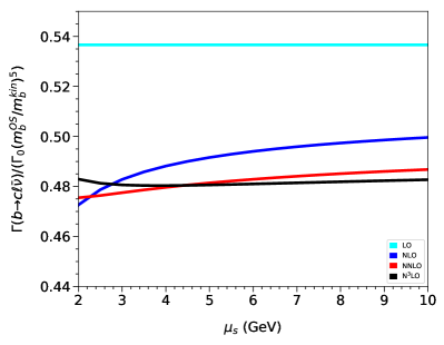
(a)

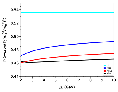
(b)

Figure 3: Total partonic decay rate in the kinetic (a) and 1S scheme (b) as a function of the renormalization scale $\mu_{s}$. See text for details. Note that the normalization chosen for the $y$ axis is scheme independent.

In general the large-$\beta_{0}$ terms provide dominant contributions. However, in all cases the remaining terms are not negligible and often have a different sign. In the kinetic scheme where the charm quark is renormalized in the $\overline{\rm MS}$ scheme the remaining contributions are numerically even bigger than the large-$\beta_{0}$ terms.

It is impressive that the expansion in $\delta$ shows a good converge behaviour even for $\delta\to 1$ which corresponds to a massless daughter quark. This allows us to extract the coefficient $X_{3}$ for the decay $b\to u\ell\bar{\nu}$. A closer look to the $\delta^{10}$, $\delta^{11}$, and $\delta^{12}$ terms in Fig. 2 indicates that the convergence is quite slow for $\rho\to 0$. As central value for the three-loop prediction we use our approximation based on the $\delta^{12}$ term and estimate the uncertainty from the behaviour of the one- and two-loop vanRitbergen:1999gs ; Steinhauser:1999bx results for $\rho=0$, where the exact results are known. Incorporating expansion terms up to order $\delta^{12}$ we observe a deviation of about 3.5% whereas the $\delta^{12}$ terms amount to less than 1%, both at one and two loops. At three loops the $\delta^{12}$ term amounts to about 2%. We thus conservatively estimate the uncertainty to 10% which leads to

$$X_{3}^{u} \approx -202\pm 20\,.$$ (10)

In this result the contributions with closed charm loops are approximated with $m_{c}=0$.

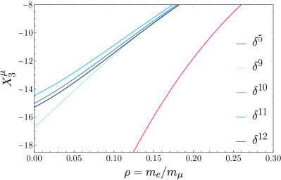
Figure 4: The third-order coefficient to $\Delta q$ introduced in Eq. (1) as a function of $m_{e}/m_{\mu}$.

In the remaining part of this paper we specify our results to QED and study the corrections to the muon decay. A comprehensive review of the various correction terms is given in Ref. vanRitbergen:1999fi where $\Delta q$ in Eq. (1) is parameterized as

$$\Delta q = \sum_{i\geq 0}\Delta q^{(i)}\,.$$ (11)

$\Delta q^{(0)}$ is given by $X_{0}-1$ (see Eq. (4)) with $\rho=m_{e}/m_{\mu}$ and $\Delta q^{(1)}$ Kinoshita:1958ru and $\Delta q^{(2)}$ vanRitbergen:1998yd ; Steinhauser:1999bx are easily obtained after specification of the QCD colour factors to their QED values (see Ref. vanRitbergen:1999fi for analytic results). We introduce $\Delta q^{(3)}=(\alpha(m_{\mu})/\pi)^{3}X_{3}^{\mu}$, where $\alpha(m_{\mu})$ is the fine structure constant in the $\overline{\rm MS}$ scheme vanRitbergen:1999fi . In Fig. 4 we show the third-order coefficient $X_{3}^{\mu}$ for $0\leq\rho\leq 0.3$. At the physical point $m_{e}/m_{\mu}\approx 0.005$ the convergence behaviour is similar to QCD. We estimate $X_{3}^{\mu}$ using the same approach as for $X_{3}^{u}$ and examine the one- and two-loop behaviour. Up to an overall factor $C_{F}$ the one-loop term is, of course, identical to the $b\to u$ transition. Including expansion terms up to $\delta^{12}$ at two loops leads to a deviation by about 8% from the exact result whereas the $\delta^{12}$ term itself contributes by about 1%. The three-loop $\delta^{12}$ amounts to about 2%. Assuming the same relative contribution thus leads to an uncertainty estimate of about 15% and we have

$$\Delta q^{(3)} \approx \left(\frac{\alpha(m_{\mu})}{\pi}\right)^{3}\left(-15.3\pm 2.3\right)\,.$$ (12)

In Ref. Ferroglia:1999tg the three-loop corrections were estimated to $X^{\mu}_{3}\sim-20$. With the help of Eq. (1) we obtain for the $\alpha^{3}$ QED contribution to the muon life time ${(-9\pm 1)\times 10^{-8}}$ $\mu$s. This result has to be compared to the current experimental value which is given by $\tau_{\mu}=2.1969811\pm 0.0000022$ $\mu$s Tanabashi:2018oca . The new correction terms are almost two orders of magnitude smaller than the experimental uncertainty. Thus, an updated value of $G_{F}$ can only be extracted once the latter has been improved.

IV Conclusions

We have computed three-loop corrections of order $\alpha_{s}^{3}$ to the total decay rate $\Gamma(B\to X_{c}\ell\bar{\nu})$ including finite charm quark mass effects. We perform an expansion around the equal-mass case and demonstrate that a good convergence at the physical point is observed after taking into account eight expansion terms. Our result is one of the very few third-order results to physical quantities available to date involving two different mass scales.

We can extend our considerations to the case of a massless charm quark and thus obtain corrections of order $\alpha_{s}^{3}$ to $\Gamma(B\to X_{u}\ell\bar{\nu})$, although with a larger uncertainty of about $10\%$. After specifying our findings to QED we furthermore obtain predictions for the third-order corrections to the muon decay. Here we estimate the uncertainty to 15%.

The decay rate $\Gamma(B\to X_{c}\ell\bar{\nu})$ is an important ingredient for the determination of the CKM matrix element $|V_{cb}|$. However, a detailed analysis (see, e.g., Ref. Alberti:2014yda ) also requires the knowledge of moments of kinematic distributions. The method described in this paper can also be applied to the calculation of such moments at order $\alpha_{s}^{3}$, although at the cost of significantly increased computer resources.

Acknowledgements. We thank Paolo Gambino for communications and clarifications concerning Ref. Alberti:2014yda . We are grateful to Alexander Smirnov for his support in the use of FIRE and to Florian Herren for providing us his program LIMIT Herren:2020ccq which automates the partial fraction decomposition in case of linearly dependent denominators. We thanks Joshua Davies for valuable advice in optimizing the usage of FORM Ruijl:2017dtg . This research was supported by the Deutsche Forschungsgemeinschaft (DFG, German Research Foundation) under grant 396021762 — TRR 257 “Particle Physics Phenomenology after the Higgs Discovery”.

References

- (1) P. Gambino and C. Schwanda, Phys. Rev. D 89 (2014) no.1, 014022 [arXiv:1307.4551 [hep-ph]].
- (2) A. Alberti, P. Gambino, K. J. Healey and S. Nandi, Phys. Rev. Lett. 114 (2015) no.6, 061802 [arXiv:1411.6560 [hep-ph]].
- (3) P. Gambino, K. J. Healey and S. Turczyk, Phys. Lett. B 763 (2016), 60-65 [arXiv:1606.06174 [hep-ph]]
- (4) P. Urquijo et al. [Belle], Phys. Rev. D 75 (2007), 032001 [arXiv:hep-ex/0610012 [hep-ex]].
- (5) C. Schwanda et al. [Belle], Phys. Rev. D 75 (2007), 032005 [arXiv:hep-ex/0611044 [hep-ex]].
- (6) B. Aubert et al. [BaBar], Phys. Rev. D 69 (2004), 111104 [arXiv:hep-ex/0403030 [hep-ex]].
- (7) B. Aubert et al. [BaBar], Phys. Rev. D 81 (2010), 032003 [arXiv:0908.0415 [hep-ex]].
- (8) D. Acosta et al. [CDF], Phys. Rev. D 71 (2005), 051103 [arXiv:hep-ex/0502003 [hep-ex]].
- (9) S. E. Csorna et al. [CLEO], Phys. Rev. D 70 (2004), 032002 [arXiv:hep-ex/0403052 [hep-ex]].
- (10) J. Abdallah et al. [DELPHI], Eur. Phys. J. C 45 (2006), 35-59 [arXiv:hep-ex/0510024 [hep-ex]].
- (11) Y. S. Amhis et al. [HFLAV], [arXiv:1909.12524 [hep-ex]].
- (12) C. W. Bauer, Z. Ligeti, M. Luke, A. V. Manohar and M. Trott, Phys. Rev. D 70 (2004), 094017 [arXiv:hep-ph/0408002 [hep-ph]].
- (13) J. P. Lees et al. [BaBar], Phys. Rev. D 95 (2017) no.7, 072001 [arXiv:1611.05624 [hep-ex]].
- (14) A. H. Mahmood et al. [CLEO], Phys. Rev. D 70 (2004), 032003 [arXiv:hep-ex/0403053 [hep-ex]].
- (15) H. Albrecht et al. [ARGUS], Phys. Lett. B 318 (1993), 397-404
- (16) E. Kou et al. [Belle-II], PTEP 2019 (2019) no.12, 123C01 [erratum: PTEP 2020 (2020) no.2, 029201] [arXiv:1808.10567 [hep-ex]].
- (17) R. van Tonder, Belle coll. “Inclusive determination of at Belle”, Moriond EW 2021.
- (18) F. Abudinén et al. [Belle-II], [arXiv:2009.04493 [hep-ex]].
- (19) M. E. Luke, M. J. Savage and M. B. Wise, Phys. Lett. B 345 (1995), 301-306 [arXiv:hep-ph/9410387 [hep-ph]].
- (20) M. Trott, Phys. Rev. D 70 (2004), 073003 [arXiv:hep-ph/0402120 [hep-ph]].
- (21) V. Aquila, P. Gambino, G. Ridolfi and N. Uraltsev, Nucl. Phys. B 719 (2005), 77-102 [arXiv:hep-ph/0503083 [hep-ph]].
- (22) A. Pak and A. Czarnecki, Phys. Rev. Lett. 100 (2008), 241807 [arXiv:0803.0960 [hep-ph]].
- (23) A. Pak and A. Czarnecki, Phys. Rev. D 78 (2008), 114015 [arXiv:0808.3509 [hep-ph]].
- (24) K. Melnikov, Phys. Lett. B 666 (2008), 336-339 [arXiv:0803.0951 [hep-ph]].
- (25) S. Biswas and K. Melnikov, JHEP 02 (2010), 089 [arXiv:0911.4142 [hep-ph]].
- (26) P. Gambino, JHEP 09 (2011), 055 [arXiv:1107.3100 [hep-ph]].
- (27) M. Dowling, J. H. Piclum and A. Czarnecki, Phys. Rev. D 78 (2008), 074024 [arXiv:0810.0543 [hep-ph]].
- (28) P. Ball, M. Beneke and V. M. Braun, Phys. Rev. D 52 (1995), 3929-3948 [arXiv:hep-ph/9503492 [hep-ph]].
- (29) J. Chay, H. Georgi and B. Grinstein, Phys. Lett. B 247 (1990), 399-405.
- (30) I. I. Y. Bigi, M. A. Shifman, N. G. Uraltsev and A. I. Vainshtein, Phys. Rev. Lett. 71 (1993), 496-499 [arXiv:hep-ph/9304225 [hep-ph]].
- (31) A. V. Manohar and M. B. Wise, Phys. Rev. D 49 (1994), 1310-1329 [arXiv:hep-ph/9308246 [hep-ph]].
- (32) M. Gremm and A. Kapustin, Phys. Rev. D 55 (1997), 6924-6932 [arXiv:hep-ph/9603448 [hep-ph]].
- (33) T. Becher, H. Boos and E. Lunghi, JHEP 12 (2007), 062 [arXiv:0708.0855 [hep-ph]].
- (34) A. Alberti, P. Gambino and S. Nandi, JHEP 01 (2014), 147 [arXiv:1311.7381 [hep-ph]].
- (35) T. Mannel, A. A. Pivovarov and D. Rosenthal, Phys. Lett. B 741 (2015), 290-294 [arXiv:1405.5072 [hep-ph]].
- (36) T. Mannel and A. A. Pivovarov, Phys. Rev. D 100 (2019) no.9, 093001 [arXiv:1907.09187 [hep-ph]].
- (37) B. M. Dassinger, T. Mannel and S. Turczyk, JHEP 03 (2007), 087 [arXiv:hep-ph/0611168 [hep-ph]].
- (38) T. Mannel, S. Turczyk and N. Uraltsev, JHEP 11 (2010), 109 [arXiv:1009.4622 [hep-ph]].
- (39) T. Mannel and K. K. Vos, JHEP 06 (2018), 115 [arXiv:1802.09409 [hep-ph]].
- (40) M. Fael, T. Mannel and K. Keri Vos, JHEP 02 (2019), 177 [arXiv:1812.07472 [hep-ph]].
- (41) T. Kinoshita and A. Sirlin, Phys. Rev. 113 (1959), 1652-1660
- (42) T. van Ritbergen and R. G. Stuart, Nucl. Phys. B 564 (2000), 343-390 [arXiv:hep-ph/9904240 [hep-ph]].
- (43) A. Ferroglia, G. Ossola and A. Sirlin, Nucl. Phys. B 560 (1999), 23-32 [arXiv:hep-ph/9905442 [hep-ph]].
- (44) M. Beneke and V. A. Smirnov, Nucl. Phys. B 522 (1998), 321-344 [arXiv:hep-ph/9711391 [hep-ph]].
- (45) V. A. Smirnov, Springer Tracts Mod. Phys. 250 (2012), 1-296
- (46) M. Fael, K. Schönwald and M. Steinhauser, Phys. Rev. Lett. 125 (2020) no.5, 052003 [arXiv:2005.06487 [hep-ph]].
- (47) M. Fael, K. Schönwald and M. Steinhauser, [arXiv:2011.11655 [hep-ph]].
- (48) A. V. Smirnov and F. S. Chuharev, arXiv:1901.07808 [hep-ph].
- (49) R. N. Lee, arXiv:1212.2685 [hep-ph]; R. N. Lee, J. Phys. Conf. Ser. 523 (2014) 012059 [arXiv:1310.1145 [hep-ph]].
- (50) R. N. Lee and V. A. Smirnov, JHEP 02 (2011), 102 [arXiv:1010.1334 [hep-ph]].
- (51) A. Sirlin, Nucl. Phys. B 196 (1982), 83-92
-
(52)
https://www.ttp.kit.edu/preprints/2020/ttp20-042/. - (53) J. P. Archambault and A. Czarnecki, Phys. Rev. D 70 (2004), 074016 [arXiv:hep-ph/0408021 [hep-ph]].
- (54) M. L. Czakon, A. Czarnecki and M. Dowling, [arXiv:2104.05804 [hep-ph]].
- (55) K. G. Chetyrkin and M. Steinhauser, Nucl. Phys. B 573 (2000) 617 [hep-ph/9911434].
- (56) K. Melnikov and T. v. Ritbergen, Phys. Lett. B 482 (2000) 99 [hep-ph/9912391].
- (57) M. Fael, K. Schönwald and M. Steinhauser, JHEP 10 (2020), 087 [arXiv:2008.01102 [hep-ph]].
- (58) A. Czarnecki, K. Melnikov and N. Uraltsev, Phys. Rev. Lett. 80 (1998) 3189 [hep-ph/9708372].
- (59) D. Benson, I. I. Bigi, T. Mannel and N. Uraltsev, Nucl. Phys. B 665 (2003), 367-401 [arXiv:hep-ph/0302262 [hep-ph]].
- (60) P. Gambino, P. Giordano, G. Ossola and N. Uraltsev, JHEP 10 (2007), 058 [arXiv:0707.2493 [hep-ph]].
- (61) M. Beneke, Phys. Lett. B 434 (1998) 115 [hep-ph/9804241].
- (62) A. H. Hoang, Z. Ligeti and A. V. Manohar, Phys. Rev. D 59 (1999), 074017 [arXiv:hep-ph/9811239 [hep-ph]].
- (63) A. H. Hoang, Z. Ligeti and A. V. Manohar, Phys. Rev. Lett. 82 (1999), 277-280 [arXiv:hep-ph/9809423 [hep-ph]].
- (64) A. Hoang and T. Teubner, Phys. Rev. D 60 (1999), 114027 [arXiv:hep-ph/9904468 [hep-ph]].
- (65) F. Herren and M. Steinhauser, Comput. Phys. Commun. 224 (2018), 333-345 [arXiv:1703.03751 [hep-ph]].
- (66) T. van Ritbergen, Phys. Lett. B 454 (1999), 353-358 [arXiv:hep-ph/9903226 [hep-ph]].
- (67) M. Steinhauser and T. Seidensticker, Phys. Lett. B 467 (1999), 271-278 [arXiv:hep-ph/9909436 [hep-ph]].
- (68) T. van Ritbergen and R. G. Stuart, Phys. Rev. Lett. 82 (1999), 488-491 [arXiv:hep-ph/9808283 [hep-ph]].
- (69) M. Tanabashi et al. [Particle Data Group], Phys. Rev. D 98 (2018) no.3, 030001
- (70) F. Herren, “Precision Calculations for Higgs Boson Physics at the LHC - Four-Loop Corrections to Gluon-Fusion Processes and Higgs Boson Pair-Production at NNLO,”, PhD thesis, KIT, 2020.
- (71) B. Ruijl, T. Ueda and J. Vermaseren, [arXiv:1707.06453 [hep-ph]].