Self-Supervised Time Series Representation Learning by Inter-Intra Relational Reasoning

Abstract

Self-supervised learning achieves superior performance in many domains by extracting useful representations from the unlabeled data. However, most of traditional self-supervised methods mainly focus on exploring the inter-sample structure while less efforts have been concentrated on the underlying intra-temporal structure, which is important for time series data. In this paper, we present SelfTime: a general Self-supervised Time series representation learning framework, by exploring the inter-sample relation and intra-temporal relation of time series to learn the underlying structure feature on the unlabeled time series. Specifically, we first generate the inter-sample relation by sampling positive and negative samples of a given anchor sample, and intra-temporal relation by sampling time pieces from this anchor. Then, based on the sampled relation, a shared feature extraction backbone combined with two separate relation reasoning heads are employed to quantify the relationships of the sample pairs for inter-sample relation reasoning, and the relationships of the time piece pairs for intra-temporal relation reasoning, respectively. Finally, the useful representations of time series are extracted from the backbone under the supervision of relation reasoning heads. Experimental results on multiple real-world time series datasets for time series classification task demonstrate the effectiveness of the proposed method. Code and data are publicly available at https://haoyfan.github.io/.

1 Introduction

Time series data is ubiquitous and there has been significant progress for time series analysis (Das, 1994) in machine learning, signal processing, and other related areas, with many real-world applications such as healthcare (Stevner et al., 2019), industrial diagnosis (Kang et al., 2015), and financial forecasting (Sen et al., 2019).

Deep learning models have emerged as successful models for time series analysis (Hochreiter & Schmidhuber, 1997; Graves et al., 2013; Shukla & Marlin, 2019; Fortuin et al., 2019; Oreshkin et al., 2020). Despite their fair share of success, the existing deep supervised models are not suitable for high-dimensional time series data with a limited amount of training samples as those data-driven approaches rely on finding ground truth for supervision, where data labeling is a labor-intensive and time-consuming process, and sometimes impossible for time series data. One solution is to learn useful representations from unlabeled data, which can substantially reduce dependence on costly manual annotation.

Self-supervised learning aims to capture the most informative properties from the underlying structure of unlabeled data through the self-generated supervisory signal to learn generalized representations. Recently, self-supervised learning has attracted more and more attention in computer vision by designing different pretext tasks on image data such as solving jigsaw puzzles (Noroozi & Favaro, 2016), inpainting (Pathak et al., 2016), rotation prediction(Gidaris et al., 2018), and contrastive learning of visual representations(Chen et al., 2020), and on video data such as object tracking (Wang & Gupta, 2015), and pace prediction (Wang et al., 2020). Although some video-based approaches attempt to capture temporal information in the designed pretext task, time series is far different structural data compared with video. More recently, in the time series analysis domain, some metric learning based self-supervised methods such as triplet loss (Franceschi et al., 2019) and contrastive loss (Schneider et al., 2019; Saeed et al., 2020), or multi-task learning based self-supervised methods that predict different handcrafted features (Pascual et al., 2019a; Ravanelli et al., 2020) and different signal transformations (Saeed et al., 2019; Sarkar & Etemad, 2020) have emerged. However, few of those works consider the intra-temporal structure of time series. Therefore, how to design an efficient pretext task in a self-supervised manner for time series representation learning is still an open problem.

In this work, we present SelfTime: a general self-supervised time series representation learning framework. Inspired by relational discovery during self-supervised human learning, which attempts to discover new knowledge by reasoning the relation among entities (Goldwater et al., 2018; Patacchiola & Storkey, 2020), we explore the inter-sample relation reasoning and intra-temporal relation reasoning of time series to capture the underlying structure pattern of the unlabeled time series data. Specifically, as shown in Figure 1, for inter-sample relation reasoning, given an anchor sample, we generate from its transformation counterpart and another individual sample as the positive and negative samples respectively. For intra-temporal relation reasoning, we firstly generate an anchor piece, then, several reference pieces are sampled to construct different scales of temporal relation between the anchor piece and the reference piece, where relation scales are determined based on the temporal distance. Note that in Figure 1, we only show an example of 3-scale temporal relations including short-term, middle-term, and long-term relation for an illustration, whereas in different scenarios, there could be different temporal relation scale candidates. Based on the sampled relation, a shared feature extraction backbone combined with two separate relation reasoning heads are employed to quantify the relationships between the sample pairs or the time piece pairs for inter-sample relation reasoning or intra-temporal relation reasoning, respectively. Finally, the useful representations of time series are extracted from the backbone under the supervision of relation reasoning heads on the unlabeled data. Overall, SelfTime is simple yet effective by conducting the designed pretext tasks directly on the original input signals.

Our main contributions are three-fold: (1) we present a general self-supervised time series representation learning framework by investigating different levels of relations of time series data including inter-sample relation and intra-temporal relation. (2) We design a simple and effective intra-temporal relation sampling strategy to capture the underlying temporal patterns of time series. (3) We conduct extensive experiments on different categories of real-world time series data, and systematically study the impact of different data augmentation strategies and temporal relation sampling strategies on self-supervised learning of time series. By comparing with multiple state-of-the-art baselines, experimental results show that SelfTime builds new state-of-the-art on self-supervised time series representation learning.

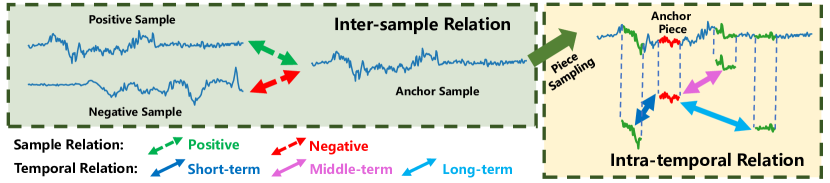
Figure 1: Exploring inter-sample relation, and multi-scale intra-temporal relation of time series. Here, an example of 3-scale temporal relations including short-term, middle-term and long-term temporal relation is given for illustration.

2 Related Work

Time Series Modeling. In the last decades, time series modeling has been paid close attention with numerous efficient methods, including distance-based methods, feature-based methods, ensemble-based methods, and deep learning based methods. Distance-based methods (Berndt & Clifford, 1994; Górecki & Łuczak, 2014) try to measure the similarity between time series using Euclidean distance or Dynamic Time Warping distance, and then conduct classification based on 1-NN classifiers. Feature-based methods aim to extract useful feature for time series representation. Two typical types including bag-of-feature based methods (Baydogan et al., 2013; Schäfer, 2015) and shapelet based methods (Ye & Keogh, 2009; Hills et al., 2014). Ensemble-based methods (Lines & Bagnall, 2015; Bagnall et al., 2015) aims at combining multiple classifiers for higher classification performance. More recently, deep learning based methods (Karim et al., 2017; Ma et al., 2019; Cheng et al., 2020) conduct classification by cascading the feature extractor and classifier based on MLP, RNN, and CNN in an end-to-end manner. Our approach focuses instead on self-supervised representation learning of time series on unlabeled data, exploiting inter-sample relation and intra-temporal relation of time series to guide the generation of useful feature.

Relational Reasoning. Reasoning the relations between entities and their properties makes significant sense to generally intelligent behavior (Kemp & Tenenbaum, 2008). In the past decades, there has been an extensive researches about relational reasoning and its applications including knowledge base (Socher et al., 2013), question answering (Johnson et al., 2017; Santoro et al., 2017), video action recognition (Zhou et al., 2018), reinforcement learning (Zambaldi et al., 2019), and graph representation (Battaglia et al., 2018), which perform relational reasoning directly on the constructed sets or graphs that explicitly represent the target entities and their relations. Different from those previous works that attempt to learn a relation reasoning head for a special task, inter-sample relation reasoning based on unlabeled image data is employed in (Patacchiola & Storkey, 2020) to learn useful visual representation in the underlying backbone. Inspired by this, in our work, we focus on time series data by exploring both inter-sample and intra-temporal relation for time series representation in a self-supervised scenario.

Self-supervised Learning. Self-supervised learning has attracted lots of attention recently in different domains including computer vision, audio/speech processing, and time series analysis. For image data, the pretext tasks including solving jigsaw puzzles (Noroozi & Favaro, 2016), rotation prediction (Gidaris et al., 2018), and visual contrastive learning (Chen et al., 2020) are designed for self-supervised visual representation. For video data, the pretext tasks such as frame order validation (Misra et al., 2016; Wei et al., 2018), and video pace prediction (Wang et al., 2020) are designed which considering additional temporal signal of video. Different from video signal that includes plenty of raw feature in both spatial and temporal dimension, time series is far different structural data with less raw features at each time point. For time series data such as audio and ECG, the metric learning based methods such as triplet loss (Franceschi et al., 2019) and contrastive loss (Schneider et al., 2019; Saeed et al., 2020), or multi-task learning based methods that predict different handcrafted features such as MFCCs, prosody, and waveform (Pascual et al., 2019a; Ravanelli et al., 2020), and different transformations of raw signal (Sarkar & Etemad, 2020; Saeed et al., 2019) have emerged recently. However, few of those works consider the intra-temporal structure of time series. Therefore, how to design an efficient self-supervised pretext task to capture the underlying structure of time series is still an open problem.

3 Method

Given an unlabeled time series set $\mathcal{T}=\{\bm{t}_{n}\}_{n=1}^{N}$, where each time series $\bm{t}_{n}=(t_{n,1},...t_{n,T})^{\mathrm{T}}$ contains $T$ ordered real values. We aim to learn a useful representation $z_{n}=f_{\theta}(\bm{t}_{n})$ from the backbone encoder $f_{\theta}(\cdot)$ where $\theta$ is the learnable weights of the neural networks. The architecture of the proposed SelfTime is shown in Figure 2, which consists of an inter-sample relational reasoning branch and an intra-temporal relational reasoning branch. Firstly, taking the original time series signals and their sampled time pieces as the inputs, a shared backbone encoder $f_{\theta}(\cdot)$ extracts time series feature and time piece feature to aggregate the inter-sample relation feature and intra-temporal relation feature respectively, and then feeds them to two separate relation reasoning heads $r_{\mu}(\cdot)$ and $r_{\varphi}(\cdot)$ to reason the final relation score of inter-sample relation and intra-temporal relation.

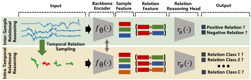
Figure 2: Architecture of SelfTime.

3.1 Inter-sample Relation Reasoning

Formally, given any two different time series samples $\bm{t}_{m}$ and $\bm{t}_{n}$ from $\mathcal{T}$, we randomly generate two sets of $K$ augmentations $\mathcal{A}(\bm{t}_{m})=\{\bm{t}_{m}^{(i)}\}_{i=1}^{K}$ and $\mathcal{A}(\bm{t}_{n})=\{\bm{t}_{n}^{(i)}\}_{i=1}^{K}$, where $\bm{t}_{m}^{(i)}$ and $\bm{t}_{n}^{(i)}$ are the $i$-th augmentations of $\bm{t}_{m}$ and $\bm{t}_{n}$ respectively. Then, we construct two types of relation pairs: positive relation pairs and negative relation pairs. A positive relation pair is $(\bm{t}_{m}^{(i)},\bm{t}_{m}^{(j)})$ sampled from the same augmentation set $\mathcal{A}(\bm{t}_{m})$, while a negative relation pair is $(\bm{t}_{m}^{(i)},\bm{t}_{n}^{(j)})$ sampled from different augmentation sets $\mathcal{A}(\bm{t}_{m})$ and $\mathcal{A}(\bm{t}_{n})$. Based on the sampled relation pairs, we use the backbone encoder $f_{\theta}$ to learn the relation representation as follows: Firstly, we extract sample representations $\bm{z}_{m}^{(i)}=f_{\theta}(\bm{t}_{m}^{(i)})$, $\bm{z}_{m}^{(j)}=f_{\theta}(\bm{t}_{m}^{(j)})$, and $\bm{z}_{n}^{(j)}=f_{\theta}(\bm{t}_{n}^{(j)})$. Then, we construct the positive relation representation $[\bm{z}_{m}^{(i)},\bm{z}_{m}^{(j)}]$, and the negative relation representation $[\bm{z}_{m}^{(i)},\bm{z}_{n}^{(j)}]$, where $[\cdot,\cdot]$ denotes the vector concatenation operation. Next, the inter-sample relation reasoning head $r_{\mu}(\cdot)$ takes the generated relation representation as input to reason the final relation score $h_{2m-1}^{(i,j)}=r_{\mu}([\bm{z}_{m}^{(i)},\bm{z}_{m}^{(j)}])$ for positive relation and $h_{2m}^{(i,j)}=r_{\mu}([\bm{z}_{m}^{(i)},\bm{z}_{n}^{(j)}])$ for negative relation, respectively. Finally, the inter-sample relation reasoning task is formulated as a binary classification task and the model is trained with binary cross-entropy loss $\mathcal{L}_{inter}$ as follows:

$$\mathcal{L}_{inter}=-\sum_{n=1}^{2N}\sum_{i=1}^{K}\sum_{j=1}^{K}(y_{n}^{(i,j)}\cdot\mathrm{log}(h_{n}^{(i,j)})+(1-y_{n}^{(i,j)})\cdot\mathrm{log}(1-h_{n}^{(i,j)}))$$ (1)

where $y_{n}^{(i,j)}=1$ for the positive relation and $y_{n}^{(i,j)}=0$ for the negative relation.

3.2 Intra-temporal Relation Reasoning

To capture the underlying temporal structure along the time dimension, we try to explore the intra-temporal relation among time pieces and ask the model to predict the different types of temporal relation. Formally, given a time series sample $\bm{t}_{n}=(t_{n,1},...t_{n,T})^{\mathrm{T}}$, we define an $L$-length time piece $\bm{p}_{n,u}$ of $\bm{t}_{n}$ starting at time step $u$ as a contiguous subsequence $\bm{p}_{n,u}=(t_{n,u},t_{n,u+1},...,t_{n,u+L-1})^{\mathrm{T}}$. Firstly, we sample different types of temporal relation among time pieces as follows: Randomly sample two $L$-length pieces $\bm{p}_{n,u}$ and $\bm{p}_{n,v}$ of $\bm{t}_{n}$ starting at time step $u$ and time step $v$ respectively. Then, the temporal relation between $\bm{p}_{n,u}$ and $\bm{p}_{n,v}$ is assigned based on their temporal distance $d_{u,v}$, e.g., for similarity, we define the temporal distance $d_{u,v}=|u-v|$ as the absolute value of the difference between two starting step $u$ and $v$. Next, we define $C$ types of temporal relations for each pair of pieces based on their temporal distance, e.g., for similarity, we firstly set a distance threshold as $D=\lfloor T/C\rfloor$, and then, if the distance $d_{u,v}$ of a piece pair is less than $D$, we assign the relation label as 0, if $d_{u,v}$ is greater than $D$ and less than $2D$, we assign the relation label as 1, and so on until we sample $C$ types of temporal relations. The details of the intra-temporal relation sampling algorithm are shown in Algorithm 1.

Based on the sampled time pieces and their temporal relations, we use the shared backbone encoder $f_{\theta}$ to extract the representations of time pieces firstly, where $\bm{z}_{n,u}=f_{\theta}(\bm{p}_{n,u})$ and $\bm{z}_{n,v}=f_{\theta}(\bm{p}_{n,v})$. Then, we construct the temporal relation representation as $[\bm{z}_{n,u},\bm{z}_{n,v}]$. Next, the intra-temporal relation reasoning head $r_{\varphi}(\cdot)$ takes the relation representation as input to reason the final relation score $h_{n}^{(u,v)}=r_{\varphi}([\bm{z}_{n,u},\bm{z}_{n,v}])$. Finally, the intra-temporal relation reasoning task is formulated as a multi-class classification problem and the model is trained with cross-entropy loss $\mathcal{L}_{intra}$ as follows:

$$\mathcal{L}_{intra}=-\sum_{n=1}^{N}y_{n}^{(u,v)}\cdot\mathrm{log}\frac{\mathrm{exp}(h_{n}^{(u,v)})}{\sum_{c=1}^{C}\mathrm{exp}(h_{n}^{(u,v)})}$$ (2)

Algorithm 1 Temporal Relation Sampling.

1:

2:$\bm{t}_{n}$: A $T$-length time series.

3:$\bm{p}_{n,u}$, $\bm{p}_{n,v}$: two $L$-length pieces of $\bm{t}_{n}$.

4:$C$: Number of relation classes.

5:

6:$y_{n}^{(u,v)}\in\{1,2,...,C\}$: The label of the temporal relation between $\bm{p}_{n,u}$ and $\bm{p}_{n,v}$.

7:$d_{u,v}=|u-v|,D=\lfloor T/C\rfloor$

8:if $d_{u,v}\leq D$ then

9:     $y_{n}^{(u,v)}=0$

10:else if $d_{u,v}\leq 2*D$ then

11:     $y_{n}^{(u,v)}=1$

12:     …

13:else if $d_{u,v}\leq(C-1)*D$ then

14:     $y_{n}^{(u,v)}=C-2$

15:else

16:     $y_{n}^{(u,v)}=C-1$

17:end if

18:return $y_{n}^{(u,v)}$

By jointly optimizing the inter-sample relation reasoning objective (Eq. 1) and intra-temporal relation reasoning objective (Eq. 2), the final training loss is defined as follows:

$$\mathcal{L}=\mathcal{L}_{inter}+\mathcal{L}_{intra}$$ (3)

An overview for training SelfTime is given in Algorithm 2 in Appendix A. SelfTime is an efficient algorithm compared with the traditional contrastive learning models such as SimCLR. The complexity of SimCLR is $O(N^{2}K^{2})$, while the complexity of SelfTime is $O(NK^{2})+O(NK)$, where $O(NK^{2})$ is the complexity of inter-sample relation reasoning module, and $O(NK)$ is the complexity of intra-temporal relation reasoning module. It can be seen that SimCLR scales quadratically in both training size $N$ and augmentation number $K$. However, in SelfTime, inter-sample relation reasoning module scales quadratically with the number of augmentations $K$, and linearly with the training size $N$, and intra-temporal relation reasoning module scales linearly with both augmentations and training size.

4 Experiments

4.1 Experimental Setup

Table 1: Statistics of Datasets.

2 Category	Dataset	Sample	Length	Class
Motion	CricketX	780	300	12
	UWaveGestureLibraryAll	4478	945	8
Sensor	DodgerLoopDay	158	288	7
	InsectWingbeatSound	2200	256	11
Device	MFPT	2574	1024	15
	XJTU	1920	1024	15
2

Datasets. To evaluate the effectiveness of the proposed method, in the experiment, we use three categories time series including four public datasets CricketX, UWaveGestureLibraryAll (UGLA), DodgerLoopDay (DLD), and InsectWingbeatSound (IWS) from the UCR Time Series Archive (Dau et al., 2018), along with two real-world bearing datasets XJTU and MFPT (Zhao et al., 2020). All six datasets consist of various numbers of instances, signal lengths, and number of classes. The statistics of the datasets are shown in Table 1.

Time Series Augmentation The data augmentations for time series are generally based on random transformation in two domains (Iwana & Uchida, 2020): magnitude domain and time domain. In the magnitude domain, transformations are performed on the values of time series where the values at each time step are modified but the time steps are constant. The common magnitude domain based augmentations include jittering, scaling, magnitude warping (Um et al., 2017), and cutout (DeVries & Taylor, 2017). In the time domain, transformations are performed along the time axis that the elements of the time series are displaced to different time steps than the original sequence. The common time domain based augmentations include time warping (Um et al., 2017), window slicing, and window warping (Le Guennec et al., 2016). More visualization details of different augmentations are shown in Figure 3.

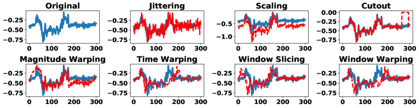
Figure 3: Data augmentations examples from CricketX dataset. The blue solid line is the original signal and the red dotted lines are the transformations.

Baselines. We compare SelfTime against several state-of-the-art methods of self-supervised representation learning:

• Supervised consists of a backbone encoder as the same with SelfTime and a linear classifier, which conducts fully supervised training over the whole networks.

• Random Weights is the same as Supervised in the architecture, but freezing the backbone’s weights during the training and optimizing only the linear classifier.

• Triplet Loss (Franceschi et al., 2019) is an unsupervised time series representation learning model that uses triplet loss to push a subsequence of time series close to its context and distant from a randomly chosen time series.

• Deep InfoMax (Hjelm et al., 2019) is a framework of unsupervised representation learning by maximizing mutual information between the input and output of a feature encoder from the local and global perspectives.

• Forecast (Jawed et al., 2020) is a semi-supervised time series classification model that leverages features learned from the self-supervised forecasting task on unlabeled data. In the experiment, we throw away the supervised classification branch and use only the forecasting branch to learn the representations of time series.

• Transformation (Sarkar & Etemad, 2020) is a self-supervised model by designing transformation recognition of different time series transformations as pretext task.

• SimCLR (Chen et al., 2020) is a simple but effective framework for self-supervised representation learning by maximizing agreement between different views of augmentation from the same sample via a contrastive loss in the latent space.

• Relation (Patacchiola & Storkey, 2020) is relational reasoning based self-supervised representation learning model by reasoning the relations between views of the sample objects as positive, and reasoning the relations between different objects as negative.

Evaluation. As a common evaluation protocol, linear evaluation is used in the experiment by training a linear classifier on top of the representations learned from different self-supervised models to evaluate the quality of the learned embeddings. For data splitting, we set the training/validation/test split as 50%/25%/25%. During the pretraining stage, we randomly split the data 5 times with different seeds, and train the backbone on them. During the linear evaluation, we train the linear classifier 10 times on each split data, and the best model on the validation dataset was used for testing. Finally, we report the classification accuracy as mean with the standard deviation across all trials.

Implementation. All experiments were performed using PyTorch (v1.4.0) (Paszke et al., 2019). A simple 4-layer 1D convolutional neural network with ReLU activation and batch normalization (Ioffe & Szegedy, 2015) were used as the backbone encoder $f_{\theta}$ for SelfTime and all other baselines, and use two separated 2-layer fully-connected networks with 256 hidden-dimensions as the inter-sample relation reasoning head $r_{\mu}$ and intra-temporal relation reasoning head $r_{\varphi}$ respectively (see Table 4 in Appendix B for details). Adam optimizer (Kingma & Ba, 2015) was used with a learning rate of 0.01 for pretraining and 0.5 for linear evaluation. The batch size is set as 128 for all models. For fair comparison, we generate $K=16$ augmentations for each sample although more augmentation results in better performance (Chen et al., 2020; Patacchiola & Storkey, 2020). More implement details of baselines are shown in Appendix D. More experimental results about the impact of augmentation number $K$ are shown in Appendix E.

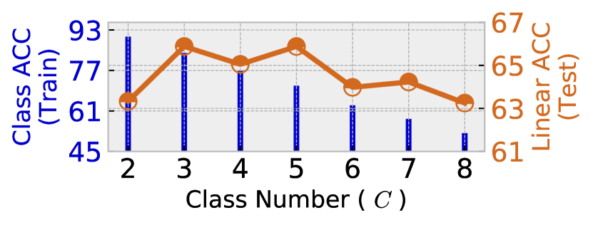
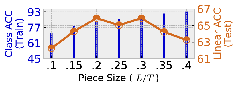
Figure 4: Impact of different temporal relation class numbers and piece sizes on CricketX dataset.

4.2 Ablation Studies

In this section, we firstly investigate the impact of different temporal relation sampling settings on intra-temporal relation reasoning. Then, we explore the effectiveness of inter-sample relation reasoning, intra-temporal relation reasoning, and their combination (SelfTime), under different time series augmentation strategies. Experimental results show that both inter-sample relation reasoning and intra-temporal relation reasoning achieve remarkable performance, which helps the network to learn more discriminating features of time series.

Temporal Relation Sampling. To investigate the different settings of temporal relation sampling strategy on the impact of linear evaluation performance, in the experiment, we set different numbers of temporal relation class $C$ and time piece length $L$. Specifically, to investigate the impact of class number, we firstly set the piece length $L=0.2*T$ as 20% of the original time series length, then, we vary $C$ from 2 to 8 during the temporal relation sampling. As shown in Figure 4, we show the results of parameter sensitivity experiments on CricketX, where blue bar indicates class reasoning accuracy on training data (Class ACC) and brown line indicates the linear evaluation accuracy on test data (Linear ACC). With the increase of class number, the Linear ACC keeps increasing until $C=5$, and we find that a small value $C=2$ and a big value $C=8$ result in worse performance. One possible reason behind this is that the increase of class number drops the Class ACC and makes the relation reasoning task too difficult for the network to learn useful representation. Similarly, when set the class number $C=3$ and vary the piece length $L$ from $0.1*T$ to $0.4*T$, we find that the Linear ACC grows up with the increase of piece size until $L=0.3*T$, and also, either small value or big value of $L$ will drop the evaluation performance, which makes the relation reasoning task too simple (with high Class ACC) or too difficult (with low Class ACC) and prevents the network from learning useful semantic representation. Therefore, as consistent with the observations of self-supervised studies in other domains (Pascual et al., 2019b; Wang et al., 2020), an appropriate pretext task designing is crucial for the self-supervised time series representation learning. In the experiment, to select a moderately difficult pretext task for different datasets, we set {class number ($C$), piece size ($L/T$)} as {3, 0.2} for CricketX, {4, 0.2} for UWaveGestureLibraryAll, {5, 0.35} for DodgerLoopDay, {6, 0.4} for InsectWingbeatSound, {4, 0.2} for MFPT, and {4, 0.2} for XJTU. More experimental results on other five datasets for parameter sensitivity analysis are shown in Appendix E.

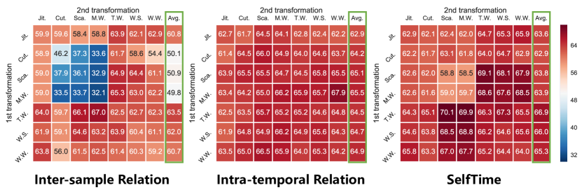
Figure 5: Linear evaluation on CricketX under individual or composition of data augmentations. For all columns but the last, diagonal entries correspond to single transformation, and off-diagonals correspond to composition of two transformations (applied sequentially). The last column reflects the average over the row.

Impact of Different Relation Modules and Data Augmentations. To explore the effectiveness of different relation reasoning modules including inter-sample relation reasoning, intra-temporal relation reasoning, and their combination (SelfTime), in the experiment, we systematically investigate the different data augmentations on the impact of linear evaluation for different modules. Here, we consider several common augmentations including magnitude domain based transformations such as jittering (Jit.), cutout (Cut.), scaling (Sca.), magnitude warping (M.W.), and time domain based transformations such as time warping (T.W.), window slicing (W.S.), window warping (W.W.). Figure 5 shows linear evaluation results on CricketX dataset under individual and composition of transformations for inter-sample relation reasoning, intra-temporal relation reasoning, and their combination (SelfTime). Firstly, we observe that the composition of different data augmentations is crucial for learning useful representations. For example, inter-sample relation reasoning is more sensitive to the augmentations, and performs worse under Cut., Sca., and M.W. augmentations, while intra-temporal relation reasoning is less sensitive to the manner of augmentations, although it performs better under the time domain based transformation. Secondly, by combining both the inter-sample and intra-temporal relation reasoning, the proposed SelfTime achieves better performance, which demonstrates the effectiveness of considering different levels of relation for time series representation learning. Thirdly, we find that the composition from a magnitude-based transformation (e.g. scaling, magnitude warping) and a time-based transformation (e.g. time warping, window slicing) facilitates the model to learn more useful representations. Therefore, in this paper, we select the composition of magnitude warping and time warping augmentations for all experiments. Similar experimental conclusions also hold on for other datasets. More experimental results on the other five datasets for evaluation of the impact of different relation modules and data augmentations are shown in Appendix F.

4.3 Time Series Classification

In this section, we evaluate the proposed method by comparing with other state-of-the-arts on time series classification task. Firstly, we conduct linear evaluation to assess the quality of the learned representations. Then, we evaluate the performance of all methods in transfer learning by training on the unlabeled source dataset and conduct linear evaluation on the labeled target dataset. Finally, we qualitatively evaluate and verify the semantic consistency of the learned representations.

Table 2: Linear evaluation of representations learned by different models on different datasets.

2 Method	Dataset
	CricketX	UGLA	DLD	IWS	MFPT	XJTU
2 Supervised	62.44$\pm$1.53	87.83$\pm$0.32	37.05$\pm$1.61	66.23$\pm$0.45	80.29$\pm$0.8	95.9$\pm$0.42
Random Weights	36.9$\pm$0.92	70.01$\pm$1.68	32.95$\pm$2.57	52.85$\pm$1.36	46.68$\pm$2.35	52.58$\pm$4.67
Triplet Loss (Franceschi et al., 2019)	40.01$\pm$2.64	71.41$\pm$1.1	41.37$\pm$2.47	53.61$\pm$2.82	47.87$\pm$2.97	53.31$\pm$3.43
Deep InfoMax (Hjelm et al., 2019)	49.16$\pm$3.03	73.88$\pm$2.37	38.95$\pm$2.47	55.99$\pm$1.31	58.99$\pm$2.72	76.27$\pm$1.83
Forecast (Jawed et al., 2020)	44.59$\pm$1.09	75.7$\pm$0.9	38.74$\pm$3.05	54.89$\pm$1.99	52.6$\pm$1.65	62.28$\pm$2.55
Transformation (Sarkar & Etemad, 2020)	52.12$\pm$2.02	75.41$\pm$0.27	35.47$\pm$1.56	59.68$\pm$1.2	60.33$\pm$3.29	85.08$\pm$2.01
SimCLR (Chen et al., 2020)	59.0$\pm$3.19	74.9$\pm$0.92	37.74$\pm$3.8	56.19$\pm$0.98	71.81$\pm$1.21	88.84$\pm$0.63
Relation (Patacchiola & Storkey, 2020)	65.3$\pm$0.43	80.87$\pm$0.78	42.84$\pm$3.23	62.0$\pm$1.49	73.53$\pm$0.65	95.14$\pm$0.72
SelfTime (ours)	68.6$\pm$0.66	84.97$\pm$0.83	49.1$\pm$2.93	66.87$\pm$0.71	78.48$\pm$0.94	96.73$\pm$0.76
2

Linear Evaluation. Following the previous studies (Chen et al., 2020; Patacchiola & Storkey, 2020), we train the backbone encoder for 400 epochs on the unlabeled training set, and then train a linear classifier for 400 epochs on top of the backbone features (the backbone weights are frozen without back-propagation). As shown in Table 2, our proposed SelfTime consistently outperforms all baselines across all datasets. SelfTime improves the accuracy over the best baseline (Relation) by 5.05% (CricketX), 5.06% (UGLA), 14.61% (DLD), 7.85% (IWS), 6.73% (MFPT), and 1.67% (XJTU) respectively. Among those baselines, either global features (Deep InfoMax, Transformation, SimCLR, Relation) or local features (Triplet Loss, Deep InfoMax, Forecast) are considered during representation learning, they neglect the essential temporal information of time series except Triplet Loss and Forecast. However, by simply forecasting future time pieces, Forecast cannot capture useful temporal structure effectively, which results in low-quality representations. Also, in Triplet Loss, a time-based negative sampling is used to capture the inter-sample temporal relation among time pieces sampled from the different time series, which is cannot directly and efficiently capture the intra-sample temporal pattern of time series. Different from all those baselines, SelfTime not only extracts global and local features by taking the whole time series and its time pieces as inputs during feature extraction, but also captures the implicit temporal structure by reasoning intra-temporal relation among time pieces.

Domain Transfer. To evaluate the transferability of the learned representations, we conduct experiments in transfer learning by training on the unlabeled source dataset and conduct linear evaluation on the labeled target dataset. In the experiment, we select two datasets from the same category as the source and target respectively. As shown in Table 3, experimental results show that our SelfTime outperforms all the other baselines under different conditions. For example, SelfTime achieves an improvement over the Relation by 4.73% on UGLA$\rightarrow$CricketX transfer, and over Deep InfoMax 20.2% on IWS$\rightarrow$DLD transfer, and over Relation 6.81% on XJTU$\rightarrow$MFPT transfer, respectively, which demonstrates the good transferability of the proposed method.

Table 3: Domain transfer evaluation by training with self-supervision on the unlabeled source data and linear evaluation on the labeled target data (e.g. source$\rightarrow$target: UGLA$\rightarrow$CricketX).

2 Method	Source$\rightarrow$Target
	UGLA$\rightarrow$CricketX	CricketX$\rightarrow$UGLA	IWS$\rightarrow$DLD	DLD$\rightarrow$IWS	XJTU$\rightarrow$MFPT	MFPT$\rightarrow$XJTU
2 Supervised	31.31$\pm$2.76	71.85$\pm$1.2	22.9$\pm$2.55	44.31$\pm$3.25	63.15$\pm$2.08	82.58$\pm$3.98
Random Weights	36.9$\pm$0.92	70.01$\pm$1.68	32.95$\pm$2.57	52.85$\pm$1.36	46.68$\pm$2.35	52.58$\pm$4.67
Triplet Loss (Franceschi et al., 2019)	30.08$\pm$4.66	55.32$\pm$2.51	34.67$\pm$3.12	45.22$\pm$3.09	53.75$\pm$2.96	59.24$\pm$3.02
Deep InfoMax (Hjelm et al., 2019)	45.92$\pm$2.3	64.2$\pm$4.19	37.42$\pm$1.99	47.75$\pm$1.74	56.75$\pm$0.77	77.14$\pm$3.14
Forecast (Jawed et al., 2020)	32.67$\pm$0.86	72.42$\pm$1.17	25.47$\pm$2.93	55.39$\pm$1.36	53.08$\pm$2.75	61.74$\pm$3.92
Transformation (Sarkar & Etemad, 2020)	39.24$\pm$2.25	70.4$\pm$1.98	30.0$\pm$1.66	57.71$\pm$0.83	54.71$\pm$1.68	69.81$\pm$8.03
SimCLR (Chen et al., 2020)	45.48$\pm$3.46	65.67$\pm$2.91	36.21$\pm$1.02	36.2$\pm$4.03	63.11$\pm$2.0	81.62$\pm$3.95
Relation (Patacchiola & Storkey, 2020)	52.55$\pm$2.67	75.67$\pm$0.54	36.0$\pm$1.52	56.29$\pm$1.82	70.27$\pm$1.14	92.77$\pm$1.15
SelfTime (ours)	55.04$\pm$2.58	77.77$\pm$0.35	45.0$\pm$1.48	57.8$\pm$1.33	75.06$\pm$1.84	93.79$\pm$2.46
2

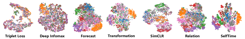
Figure 6: t-SNE visualization of the learned feature on UGLA dataset. Different colors indicate different labels.

Visualization. To qualitatively evaluate the learned representations, we use the trained backbone to extract the features and visualize them in 2D space using t-SNE (Maaten & Hinton, 2008) to verify the semantic consistency of the learned representations. Figure 6 shows the visualization results of features from the baselines and the proposed SelfTime on UGLA dataset. It is obvious that by capturing global sample structure and local temporal structure, SelfTime learns more semantic representations and results in better clustering ability for time series data, where more semantic consistency is preserved in the learned representations by our proposed method.

5 Conclusion

We presented a self-supervised approach for time series representation learning, which aims to extract useful feature from the unlabeled time series. By exploring the inter-sample relation and intra-temporal relation, SelfTime is able to capture the underlying useful structure of time series. Our main finding is that designing appropriate pretext tasks from both the global-sample structure and local-temporal structure perspectives is crucial for time series representation learning, and this finding motivates further thinking of how to better leverage the underlying structure of time series. Our experiments on multiple real-world datasets show that our proposed method consistently outperforms the state-of-the-art self-supervised representation learning models, and establishes a new state-of-the-art in self-supervised time series classification. Future directions of research include exploring more effective intra-temporal structure (i.e. reasoning temporal relation under the time point level), and extending the SelfTime to multivariate time series by considering the causal relationship among variables.

Appendix A Pseudo-code of SelfTime

The overview of training process for SelfTime is summarized in Algorithm 2.

Algorithm 2 SelfTime

1:

2:Time series set $\mathcal{T}=\{\bm{t}_{n}\}_{n=1}^{N}$.

3:$f_{\theta}$: Encoder backbone.

4:$r_{\mu}$: Inter-sample relation reasoning head.

5:$r_{\varphi}$: Intra-temporal relation reasoning head.

6:

7:$f_{\theta}$: An updated encoder backbone.

8:for $\bm{t}_{m},\bm{t}_{n}\in\mathcal{T}$ do

9:     Generate two augmentation sets $\mathcal{A}(\bm{t}_{m})$ and $\mathcal{A}(\bm{t}_{n})$

10:     Sample positive relation pair $(\bm{t}_{m}^{(i)},\bm{t}_{m}^{(j)})$ and negative   relation pair $(\bm{t}_{m}^{(i)},\bm{t}_{n}^{(j)})$ from $\mathcal{A}(\bm{t}_{m})$ and $\mathcal{A}(\bm{t}_{n})$

11:     $\bm{z}_{m}^{(i)}=f_{\theta}(\bm{t}_{m}^{(i)})$ $\triangleright$ Sample representation

12:     $\bm{z}_{m}^{(j)}=f_{\theta}(\bm{t}_{m}^{(j)})$ $\triangleright$ Sample representation

13:     $\bm{z}_{n}^{(j)}=f_{\theta}(\bm{t}_{n}^{(j)})$ $\triangleright$ Sample representation

14:     $h_{2m-1}^{(i,j)}=r_{\mu}([\bm{z}_{m}^{(i)},\bm{z}_{m}^{(j)}])$ $\triangleright$ Reasoning score of positive relation

15:     $h_{2m}^{(i,j)}=r_{\mu}([\bm{z}_{m}^{(i)},\bm{z}_{n}^{(j)}])$ $\triangleright$ Reasoning score of negative relation

16:     Sample time piece relation pair ($\bm{p}_{n,u},\bm{p}_{n,v}$) by Algorithm 1

17:     $\bm{z}_{n,u}=f_{\theta}(\bm{p}_{n,u})$ $\triangleright$ Time piece representation

18:     $\bm{z}_{n,v}=f_{\theta}(\bm{p}_{n,v})$ $\triangleright$ Time piece representation

19:     $h_{n}^{(u,v)}=r_{\varphi}([\bm{z}_{n,u},\bm{z}_{n,v}])$ $\triangleright$ Reasoning score of intra-temporal relation

20:end for

21:$\mathcal{L}_{inter}=-\sum_{n=1}^{2N}\sum_{i=1}^{K}\sum_{j=1}^{K}(y_{n}^{(i,j)}\cdot\mathrm{log}(h_{n}^{(i,j)})$  $+(1-y_{n}^{(i,j)})\cdot\mathrm{log}(1-h_{n}^{(i,j)}))$ $\triangleright$ Inter-sample relation reasoning loss

22:$\mathcal{L}_{intra}=-\sum_{n=1}^{N}y_{n}^{(u,v)}\cdot\mathrm{log}\frac{\mathrm{exp}(h_{n}^{(u,v)})}{\sum_{c=1}^{C}\mathrm{exp}(h_{n}^{(u,v)})}$ $\triangleright$ Intra-temporal relation reasoning loss

23:Update $f_{\theta}$, $r_{\mu}$, and $r_{\varphi}$ by minimizing   $\mathcal{L}=\mathcal{L}_{inter}+\mathcal{L}_{intra}$

24:return encoder backbone $f_{\theta}$, throw away $r_{\mu}$, and $r_{\varphi}$

Appendix B Architecture Diagram

SelfTime consists of a backbone encoder, a inter-sample relation reasoning head, and a intra-temporal relation reasoning head. The detail architectural diagrams of SelfTime are shown in Table 4.

Table 4: Implementation detail of SelfTime. Here, we denote 1D convolutional layer as Conv1D(in_channels, out_channels, kernel_size, stride, padding).

2	Layer Description	Output Tensor Dim.
2 #0	Input time series (or time piece)	$1\times T$ (or $1\times L$)
Backbone Encoder
#1	Conv1D(1, 8, 4, 2, 1)+BatchNorm+ReLU	$8\times T/2$ (or $8\times L/2$)
#2	Conv1D(8, 16, 4, 2, 1)+BatchNorm+ReLU	$16\times T/4$ (or $16\times L/4$)
#3	Conv1D(16, 32, 4, 2, 1)+BatchNorm+ReLU	$32\times T/8$ (or $32\times L/8$)
#4	Conv1D(32, 64, 4, 2, 1)+BatchNorm+ReLU	$64$
	+AvgPool1D+Flatten+Normalize
Inter-Sample Relation Reasoning Head
#1	Linear+BatchNorm+LeakyReLU	$256$
#2	Linear+Sigmoid	$1$
Intra-Temporal Relation Reasoning Head
#1	Linear+BatchNorm+LeakyReLU	$256$
#2	Linear+Softmax	$C$

Appendix C Data Augmentation

In this section, we list the configuration details of augmentation used in the experiment:

Jittering: We add the gaussian noise to the original time series, where noise is sampled from a Gaussian distribution $\mathcal{N}(0,0.2)$.

Scaling: We multiply the original time series with a random scalar sampled from a Gaussian distribution $\mathcal{N}(0,0.4)$.

Cutout: We replace a random 10% part of the original time series with zeros and remain the other parts unchanged.

Magnitude Warping: We multiply a warping amount determined by a cubic spline line with 4 knots on the original time series at random locations and magnitudes. The peaks or valleys of the knots are set as $\mu$ = 1 and $\sigma$ = 0.3 (Um et al., 2017).

Time Warping: We set the warping path according to a smooth cubic spline-based curve with 8 knots, where the random magnitudes is $\mu$ = 1 and a $\sigma$ = 0.2 for each knot (Um et al., 2017).

Window Slicing: We randomly crop 80% of the original time series and interpolate the cropped time series back to the original length (Le Guennec et al., 2016).

Window Warping: We randomly select a time window that is 30% of the original time series length, and then warp the time dimension by 0.5 times or 2 times (Le Guennec et al., 2016).

Appendix D Baselines

Triplet Loss (Franceschi et al., 2019) We download the authors’ official source code and use the same backbone as SelfTime, and set the number of negative samples as 10. We use Adam optimizer with learning rate 0.001 according to grid search and batch size 128 as same with SelfTime.

Deep InfoMax (Hjelm et al., 2019) We download the authors’ official source code and use the same backbone as SelfTime, and set the parameter $\alpha=0.5,\beta=1.0,\gamma=0.1$ through grid search. We use Adam optimizer with learning rate 0.0001 according grid search and batch size 128 as same with SelfTime.

Forecast (Jawed et al., 2020) Different from the original multi-task model proposed by authors, we throw away the supervised classification branch and use only the proposed forecasting branch to learn the representation in a fully self-supervised manner. We use Adam optimizer with learning rate 0.01 according to grid search and batch size 128 as same as SelfTime.

Transformation (Sarkar & Etemad, 2020) We refer to the authors’ official source code and reimplement it in PyTorch by using the same backbone and two-layer projection head as same with SelfTime. We use Adam optimizer with learning rate 0.001 according to grid search and batch size 128 as same with SelfTime.

SimCLR (Chen et al., 2020) We download the authors’ official source code by using the same backbone and two-layer projection head as same with SelfTime. We use Adam optimizer with learning rate 0.5 according grid search and batch size 128 as same as SelfTime.

Relation (Patacchiola & Storkey, 2020) We download the authors’ official source code by using the same backbone and relation module as same with SelfTime. For augmentation, we set $K=16$, and use Adam optimizer with learning rate 0.5 according to grid search and batch size 128 as same with SelfTime.

Appendix E Parameter Sensitivity

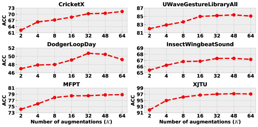
Figure 7: Impact of augmentation number $K$.

Figure 7 shows the impact of different augmentation number $K$ on all datasets. It’s obvious that more augmentations result in better performance, which demonstrates that introducing more reference samples (including positive samples and negative samples) for the anchor sample raises the power of relational reasoning.

Figure 8 shows the impact of different temporal relation class numbers and piece sizes on other five datasets: UWaveGestureLibraryAll, DodgerLoopDay, InsectWingbeatSound, MFPT, and XJTU, where the blue bar indicates class reasoning accuracy on training data (Class ACC) and the brown line indicates the linear evaluation accuracy on test data (Linear ACC). We find an interesting phenomenon is that both small values of class number $C$ or piece size $L/T$, and big values $C$ or $L/T$, result in worse performance. One possible reason behind this is that the increase of class number drops the Class ACC and makes the relation reasoning task too simple (with high Class ACC) or too difficult (with low Class ACC) and prevents the network from learning useful semantic representation. Therefore, an appropriate pretext task designing is crucial for the self-supervised time series representation learning. In the experiment, to select a moderately difficult pretext task for different datasets, we set {class number ($C$), piece size ($L/T$)} as {4, 0.2} for UWaveGestureLibraryAll, {5, 0.35} for DodgerLoopDay, {6, 0.4} for InsectWingbeatSound, {4, 0.2} for MFPT, and {4, 0.2} for XJTU.

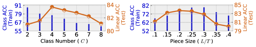
(a) UWaveGestureLibraryAll

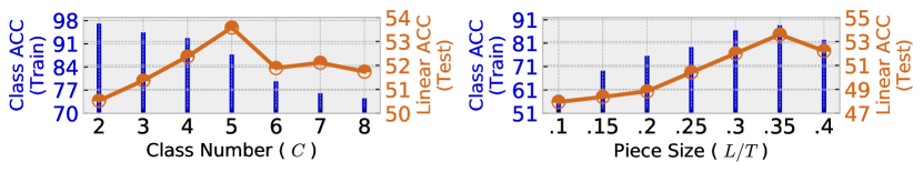
(b) DodgerLoopDay

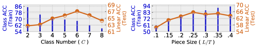
(c) InsectWingbeatSound

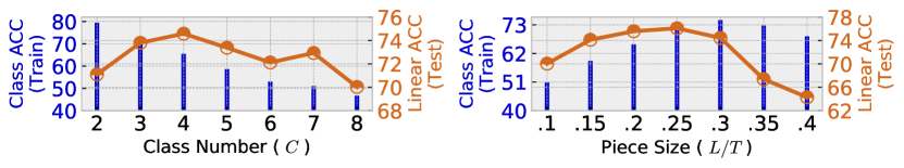
(d) MFPT

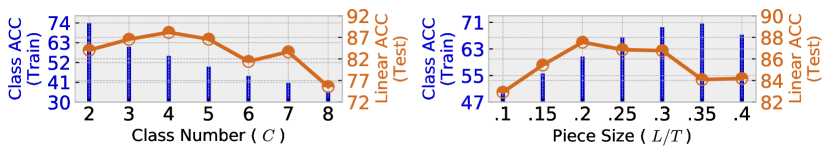
(e) XJTU

Figure 8: Impact of different temporal relation class numbers and piece sizes on other five datasets.

Appendix F Ablation Stuty

In this section, we additionally explore the effectiveness of different relation reasoning modules including inter-sample relation reasoning, intra-temporal relation reasoning, and their combination (SelfTime) on other five datasets including UWaveGestureLibraryAll, DodgerLoopDay, InsectWingbeatSound, MFPT, and XJTU. Specifically, in the experiment, we systematically investigate the different data augmentations on the impact of linear evaluation for different modules. Here, we consider several common augmentations including magnitude domain based transformations such as jittering (Jit.), cutout (Cut.), scaling (Sca.), magnitude warping (M.W.), and time domain based transformations such as time warping (T.W.), window slicing (W.S.), window warping (W.W.). Figure 9 and Figure 10 show linear evaluation results on five datasets under individual and composition of transformations for inter-sample relation reasoning, intra-temporal relation reasoning, and their combination (SelfTime). As similar to the observations from CricketX, firstly, we observe that the composition of different data augmentations is crucial for learning useful representations. For example, inter-sample relation reasoning is more sensitive to the augmentations, and performs worse under Cut., Sca., and M.W. augmentations, while intra-temporal relation reasoning is less sensitive to the manner of augmentations on all datasets. Secondly, by combining both the inter-sample and intra-temporal relation reasoning, the proposed SelfTime achieves better performance, which demonstrates the effectiveness of considering different levels of relation for time series representation learning. Thirdly, overall, we find that the composition from a magnitude-based transformation (e.g. scaling, magnitude warping) and a time-based transformation (e.g. time warping, window slicing) facilitates the model to learn more useful representations. Therefore, in this paper, we select the composition of magnitude warping and time warping augmentations for all datasets, although other compositions might result in better performance.

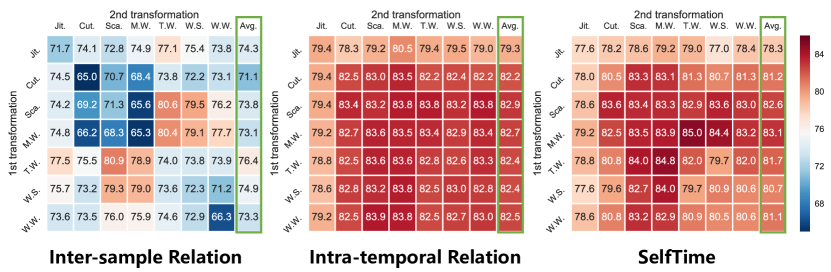
(a) UWaveGestureLibraryAll

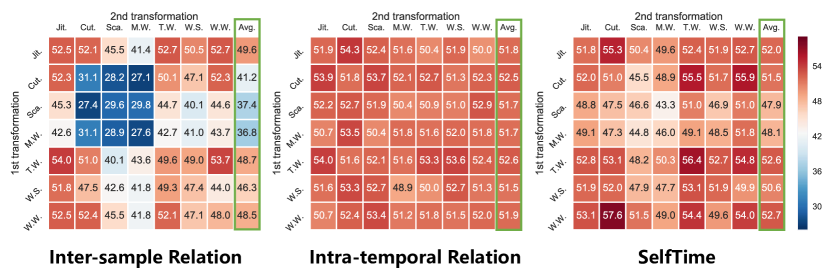
(b) DodgerLoopDay

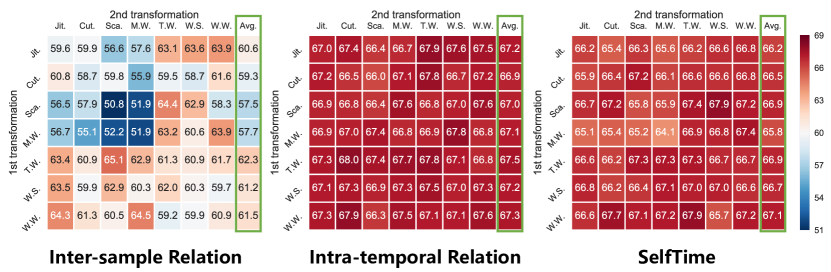
(c) InsectWingbeatSound

Figure 9: Linear evaluation on UWaveGestureLibraryAll, DodgerLoopDay, and InsectWingbeatSound datasets under individual or composition of data augmentations. For all columns but the last, diagonal entries correspond to single transformation, and off-diagonals correspond to composition of two transformations (applied sequentially). The last column reflects the average over the row.

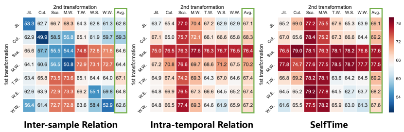
(a) MFPT

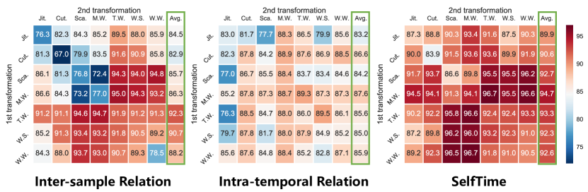
(b) XJTU

Figure 10: Linear evaluation on MFPT and XJTU datasets under individual or composition of data augmentations. For all columns but the last, diagonal entries correspond to single transformation, and off-diagonals correspond to composition of two transformations (applied sequentially). The last column reflects the average over the row.

References

- Bagnall et al. (2015) Anthony Bagnall, Jason Lines, Jon Hills, and Aaron Bostrom. Time-series classification with cote: the collective of transformation-based ensembles. IEEE Transactions on Knowledge and Data Engineering, 27(9):2522–2535, 2015.
- Battaglia et al. (2018) Peter W Battaglia, Jessica B Hamrick, Victor Bapst, Alvaro Sanchez-Gonzalez, Vinicius Zambaldi, Mateusz Malinowski, Andrea Tacchetti, David Raposo, Adam Santoro, Ryan Faulkner, et al. Relational inductive biases, deep learning, and graph networks. arXiv preprint arXiv:1806.01261, 2018.
- Baydogan et al. (2013) Mustafa Gokce Baydogan, George Runger, and Eugene Tuv. A bag-of-features framework to classify time series. IEEE transactions on pattern analysis and machine intelligence, 35(11):2796–2802, 2013.
- Berndt & Clifford (1994) Donald J Berndt and James Clifford. Using dynamic time warping to find patterns in time series. In KDD workshop, volume 10, pp. 359–370. Seattle, WA, USA:, 1994.
- Chen et al. (2020) Ting Chen, Simon Kornblith, Mohammad Norouzi, and Geoffrey Hinton. A simple framework for contrastive learning of visual representations. In Proceedings of the 37th international conference on machine learning (ICML), 2020.
- Cheng et al. (2020) Ziqiang Cheng, Yang Yang, Wei Wang, Wenjie Hu, Yueting Zhuang, and Guojie Song. Time2graph: Revisiting time series modeling with dynamic shapelets. In Proceedings of the AAAI Conference on Artificial Intelligence, AAAI, pp. 3617–3624, 2020.
- Das (1994) Samarjit Das. Time series analysis, volume 10. Princeton university press, Princeton, NJ, 1994.
- Dau et al. (2018) Hoang Anh Dau, Eamonn Keogh, Kaveh Kamgar, Chin-Chia Michael Yeh, Yan Zhu, Shaghayegh Gharghabi, Chotirat Ann Ratanamahatana, Yanping, Bing Hu, Nurjahan Begum, Anthony Bagnall, Abdullah Mueen, Gustavo Batista, and Hexagon-ML. The ucr time series classification archive, October 2018. https://www.cs.ucr.edu/~eamonn/time_series_data_2018/.
- DeVries & Taylor (2017) Terrance DeVries and Graham W Taylor. Improved regularization of convolutional neural networks with cutout. arXiv preprint arXiv:1708.04552, 2017.
- Fortuin et al. (2019) Vincent Fortuin, Matthias Hüser, Francesco Locatello, Heiko Strathmann, and Gunnar Rätsch. Som-vae: Interpretable discrete representation learning on time series. In 7th International Conference on Learning Representations, ICLR, 2019.
- Franceschi et al. (2019) Jean-Yves Franceschi, Aymeric Dieuleveut, and Martin Jaggi. Unsupervised scalable representation learning for multivariate time series. In Advances in Neural Information Processing Systems, pp. 4650–4661, 2019.
- Gidaris et al. (2018) Spyros Gidaris, Praveer Singh, and Nikos Komodakis. Unsupervised representation learning by predicting image rotations. In 6th International Conference on Learning Representations, ICLR, 2018.
- Goldwater et al. (2018) Micah B Goldwater, Hilary Don, Moritz J F Krusche, and Evan J Livesey. Relational discovery in category learning. Journal of Experimental Psychology: General, 147(1):1–35, 2018.
- Górecki & Łuczak (2014) Tomasz Górecki and Maciej Łuczak. Non-isometric transforms in time series classification using dtw. Knowledge-Based Systems, 61:98–108, 2014.
- Graves et al. (2013) Alex Graves, Abdel-rahman Mohamed, and Geoffrey Hinton. Speech recognition with deep recurrent neural networks. In 2013 IEEE international conference on acoustics, speech and signal processing, ICASSP, pp. 6645–6649, 2013.
- Hills et al. (2014) Jon Hills, Jason Lines, Edgaras Baranauskas, James Mapp, and Anthony Bagnall. Classification of time series by shapelet transformation. Data Mining and Knowledge Discovery, 28(4):851–881, 2014.
- Hjelm et al. (2019) R Devon Hjelm, Alex Fedorov, Samuel Lavoie-Marchildon, Karan Grewal, Phil Bachman, Adam Trischler, and Yoshua Bengio. Learning deep representations by mutual information estimation and maximization. In 7th International Conference on Learning Representations, ICLR, 2019.
- Hochreiter & Schmidhuber (1997) Sepp Hochreiter and Jürgen Schmidhuber. Long short-term memory. Neural computation, 9(8):1735–1780, 1997.
- Ioffe & Szegedy (2015) Sergey Ioffe and Christian Szegedy. Batch normalization: Accelerating deep network training by reducing internal covariate shift. arXiv preprint arXiv:1502.03167, 2015.
- Iwana & Uchida (2020) Brian Kenji Iwana and Seiichi Uchida. Time series data augmentation for neural networks by time warping with a discriminative teacher. arXiv preprint arXiv:2004.08780, 2020.
- Jawed et al. (2020) Shayan Jawed, Josif Grabocka, and Lars Schmidt-Thieme. Self-supervised learning for semi-supervised time series classification. In Pacific-Asia Conference on Knowledge Discovery and Data Mining, PAKDD, pp. 499–511. Springer, 2020.
- Johnson et al. (2017) Justin Johnson, Bharath Hariharan, Laurens van der Maaten, Li Fei-Fei, C Lawrence Zitnick, and Ross Girshick. Clevr: A diagnostic dataset for compositional language and elementary visual reasoning. In Proceedings of the IEEE Conference on Computer Vision and Pattern Recognition, CVPR, pp. 2901–2910, 2017.
- Kang et al. (2015) Myeongsu Kang, Jaeyoung Kim, Linda M Wills, and Jong-Myon Kim. Time-varying and multiresolution envelope analysis and discriminative feature analysis for bearing fault diagnosis. IEEE Transactions on Industrial Electronics, 62(12):7749–7761, 2015.
- Karim et al. (2017) Fazle Karim, Somshubra Majumdar, Houshang Darabi, and Shun Chen. Lstm fully convolutional networks for time series classification. IEEE access, 6:1662–1669, 2017.
- Kemp & Tenenbaum (2008) Charles Kemp and Joshua B Tenenbaum. The discovery of structural form. Proceedings of the National Academy of Sciences, 105(31):10687–10692, 2008.
- Kingma & Ba (2015) Diederik P Kingma and Jimmy Ba. Adam: A method for stochastic optimization. In 3th International Conference on Learning Representations, ICLR, 2015.
- Le Guennec et al. (2016) Arthur Le Guennec, Simon Malinowski, and Romain Tavenard. Data Augmentation for Time Series Classification using Convolutional Neural Networks. In ECML/PKDD Workshop on Advanced Analytics and Learning on Temporal Data, 2016.
- Lines & Bagnall (2015) Jason Lines and Anthony Bagnall. Time series classification with ensembles of elastic distance measures. Data Mining and Knowledge Discovery, 29(3):565–592, 2015.
- Ma et al. (2019) Qianli Ma, Wanqing Zhuang, and Garrison Cottrell. Triple-shapelet networks for time series classification. In 2019 IEEE International Conference on Data Mining (ICDM), pp. 1246–1251. IEEE, 2019.
- Maaten & Hinton (2008) Laurens van der Maaten and Geoffrey Hinton. Visualizing data using t-sne. Journal of machine learning research, 9(Nov):2579–2605, 2008.
- Misra et al. (2016) Ishan Misra, C Lawrence Zitnick, and Martial Hebert. Shuffle and learn: unsupervised learning using temporal order verification. In European Conference on Computer Vision, ECCV, pp. 527–544. Springer, 2016.
- Noroozi & Favaro (2016) Mehdi Noroozi and Paolo Favaro. Unsupervised learning of visual representations by solving jigsaw puzzles. In European Conference on Computer Vision, ECCV, pp. 69–84. Springer, 2016.
- Oreshkin et al. (2020) Boris N Oreshkin, Dmitri Carpov, Nicolas Chapados, and Yoshua Bengio. N-beats: Neural basis expansion analysis for interpretable time series forecasting. In 8th International Conference on Learning Representations, ICLR, 2020.
- Pascual et al. (2019a) Santiago Pascual, Mirco Ravanelli, Joan Serrà, Antonio Bonafonte, and Yoshua Bengio. Learning problem-agnostic speech representations from multiple self-supervised tasks. In Proc. of the Conf. of the Int. Speech Communication Association (INTERSPEECH), pp. 161–165, 2019a.
- Pascual et al. (2019b) Santiago Pascual, Mirco Ravanelli, Joan Serrà, Antonio Bonafonte, and Yoshua Bengio. Learning Problem-Agnostic Speech Representations from Multiple Self-Supervised Tasks. In Proc. of the Conf. of the Int. Speech Communication Association (INTERSPEECH), pp. 161–165, 2019b.
- Paszke et al. (2019) Adam Paszke, Sam Gross, Francisco Massa, Adam Lerer, James Bradbury, Gregory Chanan, Trevor Killeen, Zeming Lin, Natalia Gimelshein, Luca Antiga, et al. Pytorch: An imperative style, high-performance deep learning library. In Advances in neural information processing systems, NeurIPS, pp. 8026–8037, 2019.
- Patacchiola & Storkey (2020) Massimiliano Patacchiola and Amos Storkey. Self-supervised relational reasoning for representation learning. arXiv preprint arXiv:2006.05849, 2020.
- Pathak et al. (2016) Deepak Pathak, Philipp Krahenbuhl, Jeff Donahue, Trevor Darrell, and Alexei A Efros. Context encoders: Feature learning by inpainting. In Proceedings of the IEEE conference on computer vision and pattern recognition, CVPR, pp. 2536–2544, 2016.
- Ravanelli et al. (2020) Mirco Ravanelli, Jianyuan Zhong, Santiago Pascual, Pawel Swietojanski, Joao Monteiro, Jan Trmal, and Yoshua Bengio. Multi-task self-supervised learning for robust speech recognition. In IEEE International Conference on Acoustics, Speech and Signal Processing (ICASSP), pp. 6989–6993, 2020.
- Saeed et al. (2019) Aaqib Saeed, Tanir Ozcelebi, and Johan Lukkien. Multi-task self-supervised learning for human activity detection. Proceedings of the ACM on Interactive, Mobile, Wearable and Ubiquitous Technologies, 3(2):1–30, 2019.
- Saeed et al. (2020) Aaqib Saeed, Flora D Salim, Tanir Ozcelebi, and Johan Lukkien. Federated self-supervised learning of multi-sensor representations for embedded intelligence. IEEE Internet of Things Journal, 2020.
- Santoro et al. (2017) Adam Santoro, David Raposo, David G Barrett, Mateusz Malinowski, Razvan Pascanu, Peter Battaglia, and Timothy Lillicrap. A simple neural network module for relational reasoning. In Advances in neural information processing systems, NIPS, pp. 4967–4976, 2017.
- Sarkar & Etemad (2020) Pritam Sarkar and Ali Etemad. Self-supervised learning for ecg-based emotion recognition. In ICASSP 2020-2020 IEEE International Conference on Acoustics, Speech and Signal Processing (ICASSP), pp. 3217–3221. IEEE, 2020.
- Schäfer (2015) Patrick Schäfer. The boss is concerned with time series classification in the presence of noise. Data Mining and Knowledge Discovery, 29(6):1505–1530, 2015.
- Schneider et al. (2019) Steffen Schneider, Alexei Baevski, Ronan Collobert, and Michael Auli. wav2vec: Unsupervised pre-training for speech recognition. In Proc. of the Conf. of the Int. Speech Communication Association (INTERSPEECH), pp. 3465–3469, 2019.
- Sen et al. (2019) Rajat Sen, Hsiang-Fu Yu, and Inderjit S Dhillon. Think globally, act locally: A deep neural network approach to high-dimensional time series forecasting. In Advances in Neural Information Processing Systems, NeurIPS, pp. 4837–4846, 2019.
- Shukla & Marlin (2019) Satya Narayan Shukla and Benjamin M Marlin. Interpolation-prediction networks for irregularly sampled time series. In 7th International Conference on Learning Representations, ICLR, 2019.
- Socher et al. (2013) Richard Socher, Danqi Chen, Christopher D Manning, and Andrew Ng. Reasoning with neural tensor networks for knowledge base completion. In Advances in neural information processing systems, NIPS, pp. 926–934, 2013.
- Stevner et al. (2019) ABA Stevner, Diego Vidaurre, Joana Cabral, K Rapuano, Søren Føns Vind Nielsen, Enzo Tagliazucchi, Helmut Laufs, Peter Vuust, Gustavo Deco, Mark W Woolrich, et al. Discovery of key whole-brain transitions and dynamics during human wakefulness and non-rem sleep. Nature communications, 10(1):1–14, 2019.
- Um et al. (2017) Terry T Um, Franz MJ Pfister, Daniel Pichler, Satoshi Endo, Muriel Lang, Sandra Hirche, Urban Fietzek, and Dana Kulić. Data augmentation of wearable sensor data for parkinson’s disease monitoring using convolutional neural networks. In Proceedings of the 19th ACM International Conference on Multimodal Interaction, pp. 216–220, 2017.
- Wang et al. (2020) Jiangliu Wang, Jianbo Jiao, and Yun-Hui Liu. Self-supervised video representation learning by pace prediction. In European conference on computer vision, ECCV, 2020.
- Wang & Gupta (2015) Xiaolong Wang and Abhinav Gupta. Unsupervised learning of visual representations using videos. In Proceedings of the IEEE international conference on computer vision, ICCV, pp. 2794–2802, 2015.
- Wei et al. (2018) Donglai Wei, Joseph J Lim, Andrew Zisserman, and William T Freeman. Learning and using the arrow of time. In Proceedings of the IEEE Conference on Computer Vision and Pattern Recognition, CVPR, pp. 8052–8060, 2018.
- Ye & Keogh (2009) Lexiang Ye and Eamonn Keogh. Time series shapelets: a new primitive for data mining. In Proceedings of the 15th ACM SIGKDD international conference on Knowledge discovery and data mining, KDD, pp. 947–956, 2009.
- Zambaldi et al. (2019) Vinicius Zambaldi, David Raposo, Adam Santoro, Victor Bapst, Yujia Li, Igor Babuschkin, Karl Tuyls, David Reichert, Timothy Lillicrap, Edward Lockhart, et al. Deep reinforcement learning with relational inductive biases. In 7th International Conference on Learning Representations, ICLR, 2019.
- Zhao et al. (2020) Zhibin Zhao, Tianfu Li, Jingyao Wu, Chuang Sun, Shibin Wang, Ruqiang Yan, and Xuefeng Chen. Deep learning algorithms for rotating machinery intelligent diagnosis: An open source benchmark study. arXiv preprint arXiv:2003.03315, 2020.
- Zhou et al. (2018) Bolei Zhou, Alex Andonian, Aude Oliva, and Antonio Torralba. Temporal relational reasoning in videos. In Proceedings of the European Conference on Computer Vision (ECCV), pp. 803–818, 2018.